First Lidar Observations of Quasi‐Biennial Oscillation‐Induced Interannual Variations of Gravity WavePotential Energy Density at McMurdo via aModulation of the AntarcticPolar VortexZimu Li1,2 , Xinzhao Chu2 , V. Lynn Harvey3 , Jackson Jandreau2 , Xian Lu4 ,Zhibin Yu2,5 , Jian Zhao2 , and Weichun Fong2

1School of Earth and Space Sciences, University of Science and Technology of China, Hefei, China, 2Cooperative Instituteof Research in Environmental Sciences and Department of Aerospace Engineering Sciences, University of ColoradoBoulder, Boulder, CO, USA, 3Laboratory for Atmosphere and Space Physics, University of Colorado Boulder, Boulder, CO,USA, 4Department of Physics and Astronomy, Clemson University, Clemson, SC, USA, 5Harbin Institute of Technology(Shenzhen), Shenzhen, China

Abstract This work presents the first lidar observations of a Quasi‐Biennial Oscillation (QBO) in theinterannual variations of stratospheric gravity wave potential energy density (Epm in 30–50 km) atMcMurdo (77.84°S, 166.67°E), Antarctica. This paper also reports the first identification of QBO signals inthe distance between McMurdo and the polar vortex edge. Midwinter stratospheric gravity wave activity isstronger during the QBO easterly phase when the June polar vortex expands and the polar night jet shiftsequatorward. During the QBO westerly phase, gravity wave activity is weaker when the polar vortexcontracts and the polar night jet moves poleward. Nine years of lidar data (2011–2019) exhibit the mean Epmwinter maxima being ~43% higher during QBO easterly than westerly. The June polar vortex edge at 45 kmaltitude moves equatorward/poleward during QBO easterly/westerly phases with ~8° latitude differences(39.7°S vs. 47.7°S) as revealed in 21 years of MERRA‐2 data (1999–2019). We hypothesize that anequatorward shifted polar vortex corresponds to less critical level filtering of gravity waves and thus higherEpm at McMurdo. The critical level filtering is characterized by wind rotation angle (WRA), and we find alinear correlation between the WRA and Epm interannual variations. The results suggest that the QBO islikely controlling the interannual variations of the Epm winter maxima over McMurdo via the critical levelfiltering. This observationally based study lays the groundwork for a rigorous numerical study that willprovide robust statistics to better understand the mechanisms that link the tropical QBO to extratropicalwaves.

1. Introduction

Atmospheric waves, such as gravity, tidal, and planetary waves, transport momentum and energy both ver-tically and horizontally, making significant contributions to the complex coupling among stratified layersfrom the troposphere to the thermosphere, between the Northern and Southern Hemispheres, and crossingover the polar, middle, and equatorial regions (e.g., Andrews et al., 1987; Becker, 2012, 2017; Forbes, 1995;Smith, 2012a, 2012b). Insufficient and inaccurate representation of gravity waves remains one of the leadingerrors in most general circulation models and chemical climate models (e.g., Alexander et al., 2010; Garciaet al., 2014, 2017; Geller et al., 2013; Kim et al., 2003; Liu, 2019; McLandress et al., 2006; Richter et al., 2010),because, due to their small scales and wide spectra, it is still very challenging to characterize gravity waveswith observations and provide the physical basis for wave parameterizations and simulations. TheMcMurdolidar campaign conducted by the University of Colorado Boulder was designed to help address this challengeby making high‐resolution, full diurnal cycle, and all‐year‐round observations at a very high southern lati-tude of ~78°S (Chu, Huang, et al., 2011; Chu, Yu, et al., 2011). This ongoing campaign has collected datafor the last decade since late 2010. The lidar data have revealed McMurdo as a geophysical hot spot of atmo-spheric waves (e.g., Chen et al., 2013, 2016; Chen & Chu, 2017; Chu, Huang, et al., 2011; Chu, Yu, et al., 2011;Chu et al., 2018; Lu et al., 2015, 2017; Zhao et al., 2017), and the discovery of persistent gravity waves in the

©2020. American Geophysical Union.All Rights Reserved.

RESEARCH ARTICLE10.1029/2020JD032866

Key Points:• We report a Quasi‐Biennial

Oscillation in Antarctic gravity waveactivity—potential energy density isenhanced during QBO easterlywinters

• Antarctic polar vortex edge movesequatorward/poleward during QBOeasterly/westerly phases with amaximum latitude difference of ~8°in June

• An equatorward shifted polar vortexcorresponds to less critical levelfiltering of gravity waves and thushigher Epm in QBO easterly winters

Correspondence to:X. Chu,xinzhao.chu@colorado.edu

Citation:Li, Z., Chu, X., Harvey, V. L., Jandreau,J., Lu, X., Yu, Z., et al. (2020). First lidarobservations of Quasi‐BiennialOscillation‐induced interannualvariations of gravity wave potentialenergy density at McMurdo via amodulation of the Antarctic polarvortex. Journal of Geophysical Research:Atmospheres, 125, e2020JD032866.https://doi.org/10.1029/2020JD032866

Received 1 APR 2020Accepted 6 JUL 2020Accepted article online 26 JUL 2020

Author Contributions:Conceptualization: Xinzhao ChuData curation: Zimu Li, Xinzhao Chu,Zhibin Yu, Jian Zhao, Weichun FongFormal analysis: Zimu Li, XinzhaoChu, V. Lynn Harvey, JacksonJandreauInvestigation: Zimu Li, Xinzhao Chu,V. Lynn Harvey, Jackson Jandreau,Zhibin YuMethodology: Zimu Li, Xinzhao Chu,V. Lynn Harvey, Xian LuSoftware: Zimu Li, V. Lynn Harvey,Jackson Jandreau, Jian Zhao, WeichunFongValidation: Zimu Li, Xinzhao Chu, V.Lynn Harvey, Jackson JandreauWriting ‐ original draft: Xinzhao Chu(continued)

LI ET AL. 1 of 22

mesosphere and lower thermosphere (MLT) (Chen et al., 2016) have inspired systematic studies of gravitywaves from the thermosphere to the stratosphere in Antarctica.

Much has been learned about short‐term gravity wave variations over McMurdo. For example, lidar obser-vations reveal thermosphere‐ionosphere Fe (TIFe) layers with clear gravity wave signatures (periods ~1.5 hr)to at least 170 km in altitude (Chu, Yu, et al., 2011; Chu et al., 2016; Chu & Yu, 2017). Such 1.5–2 hr gravitywaves have vertical wavelengths varying from ~ 20 km to over 70 km into the thermosphere (Chen, 2016;Chu, Yu, et al., 2011; Chu et al., 2012). Gravity waves with periods of 3–10 hr dominate the temperature per-turbations in the MLT in such paramount ways (Chen et al., 2016; Chen & Chu, 2017) that no tidal signa-tures can be seen without averaging over several years of lidar data (Fong et al., 2014). Consequently,Chen et al. (2016) named these MLT waves the “persistent gravity waves.” Case studies of the persistentwaves point their sources to the stratosphere (Chen et al., 2013). Studies of stratospheric gravity waves using5 years of Fe lidar data from 2011 to 2015 exhibit a repeated seasonal pattern with summer minima and win-ter maxima in the gravity wave potential energy mass density (Epm) between 30 and 50 km (Chu et al., 2018)and the seasonal variations in the wave periods and vertical wavelengths of stratospheric dominant gravitywaves (Zhao et al., 2017). Chu et al. (2018) have found that the summer‐winter asymmetry in the Epm varia-tions are mainly caused by the critical level filtering, while the Epm variations during winter months are posi-tively correlated with the near‐surface and stratospheric winds. The derived horizontal wavelengths(~400 km) of dominant gravity waves in the stratosphere (Zhao et al., 2017) are significantly shorter thanthose (~2,000 km) of the persistent gravity waves in the MLT (Chen et al., 2013; Chen & Chu, 2017), leadingto the conclusion that dominant gravity waves in the stratosphere are starkly different from the large‐scalepersistent gravity waves in the MLT. Combining the McMurdo lidar observations (Chen et al., 2013, 2016;Chen & Chu, 2017; Chu et al., 2018; Zhao et al., 2017) with Kühlungsborn Mechanistic generalCirculation Model (KMCM) numerical simulations (Becker & Vadas, 2018; Vadas & Becker, 2018) andupdating the original theory of secondary gravity wave generation (Vadas et al., 2003), Vadas et al. (2018)proposed a “primary‐secondary” wave coupling picture in Antarctica to reconcile the observed large differ-ences between the MLT and the stratospheric gravity waves. That is, the downslope winds blowing downfrom the East Antarctic plateau onto the Ross Sea generate orographic gravity waves with considerably largeamplitudes. As these orographic gravity waves dissipate near the stratopause or in the lower mesosphere,momentum deposition results in localized and intermittent body forces. Such body forces excite the second-ary gravity waves that possess scales several times larger than the primary orographic gravity waves (Vadaset al., 2018). These large‐scale secondary gravity waves can propagate and penetrate to the lower thermo-sphere, forming the persistent gravity waves. The secondary gravity wave signatures predicted by the theoryin Vadas et al. (2018) were successfully identified in the McMurdo lidar data (Vadas et al., 2018) and in theKMCM simulations (Vadas & Becker, 2018).

Despite the above picture being quite complete in terms of short‐term variations and vertical coupling bygravity waves in Antarctica, there remain important unanswered questions concerning long‐term variationsand horizontal coupling. For example, we still do not know what factors drive the interannual variations inthe observed gravity wave Epm. Chu et al. (2018) have noted from the 5 years of data that the stratosphericEpm shows larger winter values in 2012 and 2015 than in the other three years (2011, 2013, and 2014) andsuggested that the critical level filtering may play a role; however, the causes and mechanisms remainedunresolved. Now we have learned that 2012 and 2015 correspond to the easterly phase of the equatorialQuasi‐Biennial Oscillation (QBO), while the other three years are in the westerly phase. Is the equatorialQBO responsible for the interannual variations of polar gravity waves? Signatures of the QBO at high lati-tudes have been observed since the 1960s following the discovery of the tropical oscillation (see a reviewby Anstey & Shepherd, 2014), and Holton and Tan (1980) proposed a mechanism, often referred to as theHolton‐Tan effect, to explain the dynamical coupling between low and high latitudes. It is known thatQBO can affect the polar wind and temperature fields including the Antarctic (e.g., Baldwin &Dunkerton, 1998; Ford et al., 2009; Lu et al., 2019; Yamashita et al., 2018) and that background winds impactgravity waves substantially (e.g., Becker, 2012; Fritts & Alexander, 2003); therefore, it is plausible that thetropical QBO affects the very high latitude gravity wave activity. This clue leads us to investigate the inter-annual variations of Epm and their correlation with the QBO as Part 3 of our studies of stratospheric gravitywaves at McMurdo, following Part 1 (dominant gravity wave characteristics and their seasonal variations) inZhao et al. (2017) and Part 2 (gravity wave potential energy densities and their seasonal variations) in

10.1029/2020JD032866Journal of Geophysical Research: Atmospheres

LI ET AL. 2 of 22

Writing – review & editing: Zimu Li,Xinzhao Chu, V. Lynn Harvey, JacksonJandreau, Xian Lu, Zhibin Yu

Chu et al. (2018). With the aid of 21 years (1999–2019) of reanalysis data from the Modern Era RetrospectiveAnalysis of Research and Applications, Version 2 (MERRA‐2; Bosilovich et al., 2015), we find in this studythat the Antarctic polar vortex edge exhibits an equatorward shift corresponding to the enhanced gravitywave Epm in QBO easterly June. Based on the results, we will propose an explanation for how theequatorial QBO may impact the polar gravity waves. This observational study lays the groundwork forfuture numerical studies that will provide more robust statistics to better understand the mechanisms thatlink the tropical QBO to extratropical gravity waves.

2. McMurdo Lidar Observations, MERRA‐2 Reanalysis Data, and Methodology2.1. Lidar Observational Campaign at Arrival Heights

The McMurdo lidar observation campaigns have been conducted by the University of Colorado Boulder atArrival Heights Observatory via collaboration between the United States Antarctic Program (USAP) andthe Antarctica New Zealand (AntNZ) for nearly a decade. The first Fe Boltzmann lidar (Chu et al., 2002)was installed in the AntNZ Arrival Heights building and started the data collection in December 2010(Chu, Huang, et al., 2011; Chu, Yu, et al., 2011). Seven years later the second lidar, a STAR Na Doppler lidar(Smith & Chu, 2015), was added to the same lidar lab, and simultaneous Fe and Na lidar data have been col-lected since January 2018. Nine years of Fe lidar data are chosen for this study because of their longer recordsthan the Na lidar. Atmospheric temperature profiles are derived using the Rayleigh integration technique inthe pure molecular scattering region (Hauchecorne & Chanin, 1980) and using the Fe Boltzmann techniquein the meteoric Fe layer region (Chu et al., 2002; Gelbwachs, 1994). The raw photon counts of Fe lidar werecollected in resolutions of 1 min and 48 m. To achieve sufficient signal‐to‐noise ratios (SNRs), we take thesame methodology as in Chu et al. (2018); that is, the Rayleigh temperature data were retrieved with a tem-poral integration window of 2 hr and a spatial binning window of 0.96 km, and an oversampling method wasapplied to have steps of 1 hr and 0.96 km.

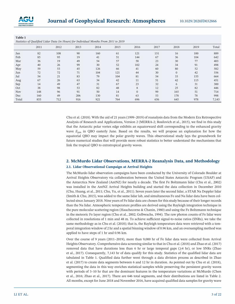
Over the course of 9 years (2011–2019), more than 9,000 hr of Fe lidar data were collected from ArrivalHeights Observatory. Comprehensive data screening similar to that in Chu et al. (2018) and Zhao et al. (2017)removed data that have durations less than 6 hr or large temporal gaps (≥4 hr), or low SNRs (Zhaoet al., 2017). Consequently, 7,143 hr of data qualify for this study. Statistics of the qualified lidar data aretabulated in Table 1. Qualified data further went through a data division process as described in Zhaoet al. (2017) to create data segments between 6 and 12 hr in duration. As pointed out by Chu et al. (2018),segmenting the data in this way enriches statistical samples while preserving the persistent gravity waveswith periods of 3–10 hr that are the dominant features in the temperature variations at McMurdo (Chenet al., 2016; Zhao et al., 2017). There are 646 total segments, and their distributions are listed in Table 2.All months, except for June 2018 and November 2016, have acquired qualified data samples for gravity wave

Table 1Statistics of Qualified Lidar Data (in Hours) for Individual Months From 2011 to 2019

2011 2012 2013 2014 2015 2016 2017 2018 2019 Total

Jan 82 108 90 160 61 121 151 16 100 889Feb 85 95 19 41 51 144 67 36 104 642Mar 36 19 49 54 57 58 23 30 77 403Apr 40 26 99 30 52 102 24 34 91 498May 59 53 45 126 66 41 60 80 52 582Jun 72 72 71 104 121 44 30 0 42 556Jul 54 21 83 79 104 81 54 33 155 664Aug 67 26 63 34 42 11 51 42 115 451Sep 14 49 47 31 67 23 32 6 31 300Oct 38 98 53 82 48 8 12 25 82 446Nov 148 96 91 50 14 0 99 165 51 714Dec 160 49 206 130 81 63 53 178 78 998Total 855 712 916 921 764 696 656 645 978 7,143

10.1029/2020JD032866Journal of Geophysical Research: Atmospheres

LI ET AL. 3 of 22

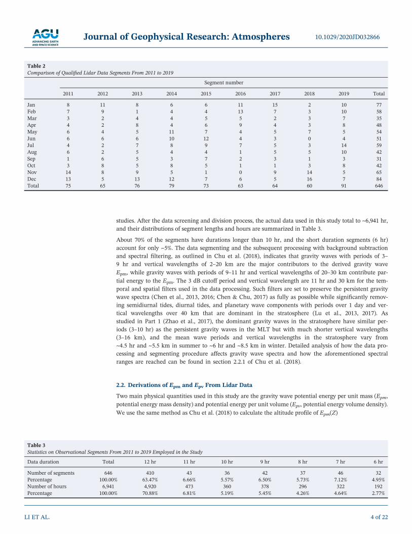
studies. After the data screening and division process, the actual data used in this study total to ~6,941 hr,and their distributions of segment lengths and hours are summarized in Table 3.

About 70% of the segments have durations longer than 10 hr, and the short duration segments (6 hr)account for only ~5%. The data segmenting and the subsequent processing with background subtractionand spectral filtering, as outlined in Chu et al. (2018), indicates that gravity waves with periods of 3–9 hr and vertical wavelengths of 2–20 km are the major contributors to the derived gravity waveEpm, while gravity waves with periods of 9–11 hr and vertical wavelengths of 20–30 km contribute par-tial energy to the Epm. The 3 dB cutoff period and vertical wavelength are 11 hr and 30 km for the tem-poral and spatial filters used in the data processing. Such filters are set to preserve the persistent gravitywave spectra (Chen et al., 2013, 2016; Chen & Chu, 2017) as fully as possible while significantly remov-ing semidiurnal tides, diurnal tides, and planetary wave components with periods over 1 day and ver-tical wavelengths over 40 km that are dominant in the stratosphere (Lu et al., 2013, 2017). Asstudied in Part 1 (Zhao et al., 2017), the dominant gravity waves in the stratosphere have similar per-iods (3–10 hr) as the persistent gravity waves in the MLT but with much shorter vertical wavelengths(3–16 km), and the mean wave periods and vertical wavelengths in the stratosphere vary from~4.5 hr and ~5.5 km in summer to ~6 hr and ~8.5 km in winter. Detailed analysis of how the data pro-cessing and segmenting procedure affects gravity wave spectra and how the aforementioned spectralranges are reached can be found in section 2.2.1 of Chu et al. (2018).

2.2. Derivations of Epm and Epv From Lidar Data

Two main physical quantities used in this study are the gravity wave potential energy per unit mass (Epm,potential energy mass density) and potential energy per unit volume (Epv, potential energy volume density).We use the same method as Chu et al. (2018) to calculate the altitude profile of Epm(Z)

Table 2Comparison of Qualified Lidar Data Segments From 2011 to 2019

Segment number

2011 2012 2013 2014 2015 2016 2017 2018 2019 Total

Jan 8 11 8 6 6 11 15 2 10 77Feb 7 9 1 4 4 13 7 3 10 58Mar 3 2 4 4 5 5 2 3 7 35Apr 4 2 8 4 6 9 4 3 8 48May 6 4 5 11 7 4 5 7 5 54Jun 6 6 6 10 12 4 3 0 4 51Jul 4 2 7 8 9 7 5 3 14 59Aug 6 2 5 4 4 1 5 5 10 42Sep 1 6 5 3 7 2 3 1 3 31Oct 3 8 5 8 5 1 1 3 8 42Nov 14 8 9 5 1 0 9 14 5 65Dec 13 5 13 12 7 6 5 16 7 84Total 75 65 76 79 73 63 64 60 91 646

Table 3Statistics on Observational Segments From 2011 to 2019 Employed in the Study

Data duration Total 12 hr 11 hr 10 hr 9 hr 8 hr 7 hr 6 hr

Number of segments 646 410 43 36 42 37 46 32Percentage 100.00% 63.47% 6.66% 5.57% 6.50% 5.73% 7.12% 4.95%Number of hours 6,941 4,920 473 360 378 296 322 192Percentage 100.00% 70.88% 6.81% 5.19% 5.45% 4.26% 4.64% 2.77%

10.1029/2020JD032866Journal of Geophysical Research: Atmospheres

LI ET AL. 4 of 22

Epm zð Þ ¼ 12

g2

N2 zð ÞT ′

GW z; tð ÞTBkg zð Þ

� �2

¼ 12

g2

N2 zð Þ1np

∑np

i¼1

T ′

GW z; tið ÞTBkg zð Þ

� �2

(1)

where the overbar denotes taking the mean over the time span of the observational segment, the gravita-tional acceleration g ¼ 9.7 m/s2 corresponding to the stratosphere, z and t respectively represent altitude

and time, TBkg is the monthly mean background temperature, T ′

GW represents the pure temperature per-turbations induced by gravity waves, and np is the number of temperature perturbation profiles within thesegment time span. Here N(z) is the buoyancy frequency calculated from the segment temporal mean tem-peratures T0(Z) through

N2 zð Þ ¼ −g

T0 zð ÞdT0 zð Þdz

þ gCp

� �(2)

where Cp ¼ 1,004 J/K/kg is the specific heat of dry air at constant pressure. We also compute the altitudeprofile of Epv(z), for each observational segment, by multiplying Epm(z) with the background atmosphericdensity ρ0(z):

Epv zð Þ ¼ ρ0 zð ÞEpm zð Þ (3)

The procedures of deriving Epm and Epv from temperature profiles are quite involved, as the key stepsinclude (1) deriving gravity wave‐induced temperature perturbations from the raw temperature data, and(2) accurately estimating the energy of gravity waves from the derived perturbations (Chu et al., 2018).The major challenges are how to retain gravity wave‐induced perturbations while removing the influencesfrom other atmospheric waves (such as tides and planetary waves) and how to remove the contributionsfrom noise variance to the total energy density. Chu et al. (2018) have done extensive investigations intothese issues and provided thorough considerations and step‐by‐step procedures on the derivations. We clo-sely followed the procedures outlined in section 2.2 of Chu et al. (2018), especially the background subtrac-tion, spectral filtering, and applying the spectral proportion method to extract the potential energy densityinduced by gravity waves. Interested readers may refer to that article for more details.

2.3. MERRA‐2 Reanalysis Data and Identification of Polar Vortex Edge

The NASA MERRA‐2 reanalysis data (Bosilovich et al., 2015; Gelaro et al., 2017) provide the backgroundtemperature, zonal and meridional winds from the surface to the top boundary of 0.01 hPa (~80 km) forcharacterizing the QBO index, polar vortex edge distance and wind strength, and wind rotation angle(WRA). MERRA‐2 produces a realistic QBO in the zonal wind, meanmeridional circulation, and ozone overthe 1980–2015 time period (Coy et al., 2016). This work uses reanalysis data from 1999 to 2019 due toimproved data quality following the addition of AMSU‐A and AMSU‐B upper air radiances to the dataassimilation stream in 1999 (see Figure 8 in Fujiwara et al., 2017, where AMSU stands for AdvancedMicrowave Sounding Unit). The inclusion of Aura Microwave Limb Sounder temperatures in August2004 further improved the data quality above 5 hPa (40 km). The temporal, horizontal, and vertical resolu-tions of the MERRA‐2 data used in this work are 6 hr, 0.5° latitude by 0.625° longitude, and 1–2 km,respectively.

The distance from McMurdo Station to the polar vortex edge is derived from the MERRA‐2 reanalysis data.The method to demark the Antarctic vortex edge is described by Harvey et al. (2002) and briefly describedhere. First, the scalar field “Q” (see their Figure 1) is calculated; Q is a relative measure of strain versus rota-tion in the horizontal flow; it is negative where rotation dominates and is positive in regions of strong hor-izontal wind shear. Areas of negative Q are located inside the polar vortex, while positive Q is located at thevortex edge on the flanks of the polar night jet (PNJ) stream. The vortex edge demarcation algorithm firstintegrates Q around stream function contours starting in the center of the vortex and incrementing outward.Neighboring stream function contours in which line‐integrated Q changes sign are saved as vortex edge“candidates.” The actual vortex edge is the candidate with the fastest line‐integrated wind speed.Illustrations of vortex edge location and the corresponding wind field and PNJ will be given in sections 4and 5 (Figures 4c and 6–8). In the middle and upper stratosphere, this vortex demarcation algorithm is

10.1029/2020JD032866Journal of Geophysical Research: Atmospheres

LI ET AL. 5 of 22

slightly more conservative but in good agreement (Meek et al., 2017) with the widely used “Nash” algorithmthat is based on horizontal gradients in potential vorticity (Nash et al., 1996). In general, this method yields avortex edge that is located along the poleward flank of the PNJ stream. Thus, in this work, the distancebetween McMurdo and the edge of the vortex can also be interpreted as the distance between McMurdoand the PNJ.

3. Interannual Variations and 9‐Year Mean Annual Cycle of Epm, Epv, and N2

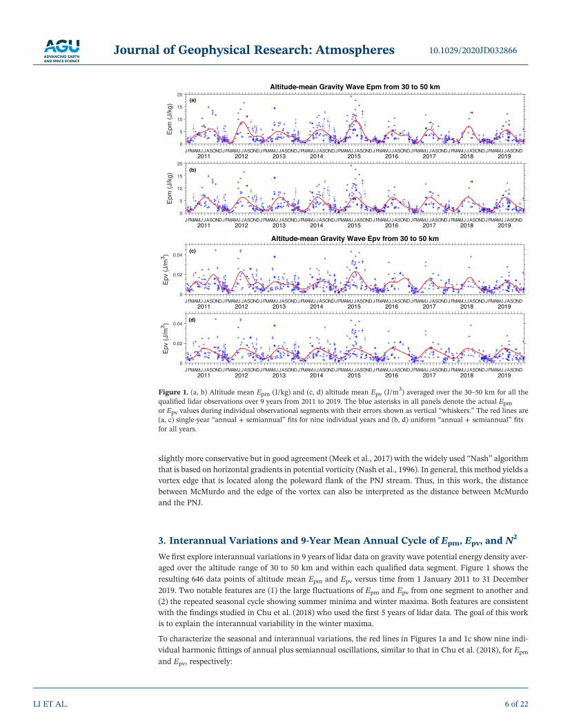
We first explore interannual variations in 9 years of lidar data on gravity wave potential energy density aver-aged over the altitude range of 30 to 50 km and within each qualified data segment. Figure 1 shows theresulting 646 data points of altitude mean Epm and Epv versus time from 1 January 2011 to 31 December2019. Two notable features are (1) the large fluctuations of Epm and Epv from one segment to another and(2) the repeated seasonal cycle showing summer minima and winter maxima. Both features are consistentwith the findings studied in Chu et al. (2018) who used the first 5 years of lidar data. The goal of this workis to explain the interannual variability in the winter maxima.

To characterize the seasonal and interannual variations, the red lines in Figures 1a and 1c show nine indi-vidual harmonic fittings of annual plus semiannual oscillations, similar to that in Chu et al. (2018), for Epmand Epv, respectively:

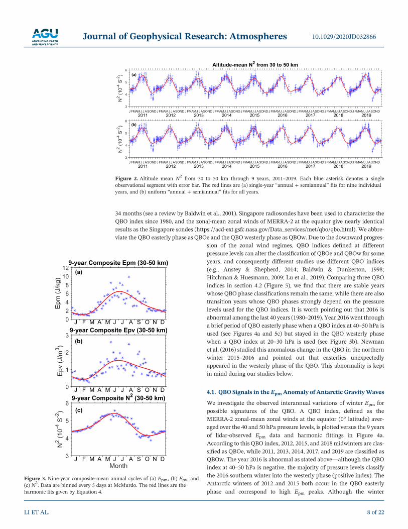
Figure 1. (a, b) Altitude mean Epm (J/kg) and (c, d) altitude mean Epv (J/m3) averaged over the 30–50 km for all thequalified lidar observations over 9 years from 2011 to 2019. The blue asterisks in all panels denote the actual Epmor Epv values during individual observational segments with their errors shown as vertical “whiskers.” The red lines are(a, c) single‐year “annual + semiannual” fits for nine individual years and (b, d) uniform “annual + semiannual” fitsfor all years.

10.1029/2020JD032866Journal of Geophysical Research: Atmospheres

LI ET AL. 6 of 22

y ¼ A0 þ A12cos2π365

x − φ12ð Þ� �

þ A6cos2π

365=2x − φ6ð Þ

� �(4)

where A0 is the annual mean, A12 and φ12 are the amplitude and phase of annual oscillation, and A6 andφ6 are the amplitude and phase of semiannual oscillation. The fitting parameters and their errors are listedin Table 4. The red curves in Figures 1b and 1d represent the uniform fittings to all years. The annualmeans A0 in 2012 and 2015 are larger than the other seven years, and the amplitudes A12 of the annualvariations in 2012, 2015, and 2018 are larger than in the other six years. The accumulated effects of largerannual means and larger annual amplitudes in the years with a QBO easterly phase are reflected in thefitted Epm curves (see Figure 1a) that show higher midwinter maxima in 2012, 2015, and 2018 than theother years.

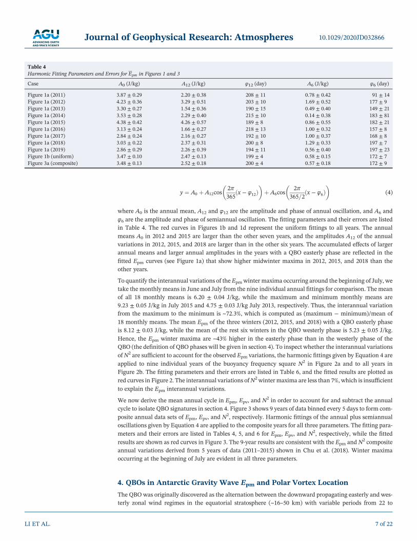
To quantify the interannual variations of the Epm winter maxima occurring around the beginning of July, wetake the monthly means in June and July from the nine individual annual fittings for comparison. The meanof all 18 monthly means is 6.20 ± 0.04 J/kg, while the maximum and minimum monthly means are9.23 ± 0.05 J/kg in July 2015 and 4.75 ± 0.03 J/kg July 2013, respectively. Thus, the interannual variationfrom the maximum to the minimum is ~72.3%, which is computed as (maximum − minimum)/mean of18 monthly means. The mean Epm of the three winters (2012, 2015, and 2018) with a QBO easterly phaseis 8.12 ± 0.03 J/kg, while the mean of the rest six winters in the QBO westerly phase is 5.23 ± 0.05 J/kg.Hence, the Epm winter maxima are ~43% higher in the easterly phase than in the westerly phase of theQBO (the definition of QBO phases will be given in section 4). To inspect whether the interannual variationsof N2 are sufficient to account for the observed Epm variations, the harmonic fittings given by Equation 4 areapplied to nine individual years of the buoyancy frequency square N2 in Figure 2a and to all years inFigure 2b. The fitting parameters and their errors are listed in Table 6, and the fitted results are plotted asred curves in Figure 2. The interannual variations ofN2 winter maxima are less than 7%, which is insufficientto explain the Epm interannual variations.

We now derive the mean annual cycle in Epm, Epv, and N2 in order to account for and subtract the annualcycle to isolate QBO signatures in section 4. Figure 3 shows 9 years of data binned every 5 days to form com-posite annual data sets of Epm, Epv, and N2, respectively. Harmonic fittings of the annual plus semiannualoscillations given by Equation 4 are applied to the composite years for all three parameters. The fitting para-meters and their errors are listed in Tables 4, 5, and 6 for Epm, Epv, and N2, respectively, while the fittedresults are shown as red curves in Figure 3. The 9‐year results are consistent with the Epm and N2 compositeannual variations derived from 5 years of data (2011–2015) shown in Chu et al. (2018). Winter maximaoccurring at the beginning of July are evident in all three parameters.

4. QBOs in Antarctic Gravity Wave Epm and Polar Vortex Location

The QBO was originally discovered as the alternation between the downward propagating easterly and wes-terly zonal wind regimes in the equatorial stratosphere (~16–50 km) with variable periods from 22 to

Table 4Harmonic Fitting Parameters and Errors for Epm in Figures 1 and 3

Case A0 (J/kg) A12 (J/kg) φ12 (day) A6 (J/kg) φ6 (day)

Figure 1a (2011) 3.87 ± 0.29 2.20 ± 0.38 208 ± 11 0.78 ± 0.42 91 ± 14Figure 1a (2012) 4.23 ± 0.36 3.29 ± 0.51 203 ± 10 1.69 ± 0.52 177 ± 9Figure 1a (2013) 3.30 ± 0.27 1.54 ± 0.36 190 ± 15 0.49 ± 0.40 149 ± 21Figure 1a (2014) 3.53 ± 0.28 2.29 ± 0.40 215 ± 10 0.14 ± 0.38 183 ± 81Figure 1a (2015) 4.38 ± 0.42 4.26 ± 0.57 189 ± 8 0.86 ± 0.55 182 ± 21Figure 1a (2016) 3.13 ± 0.24 1.66 ± 0.27 218 ± 13 1.00 ± 0.32 157 ± 8Figure 1a (2017) 2.84 ± 0.24 2.16 ± 0.27 192 ± 10 1.00 ± 0.37 168 ± 8Figure 1a (2018) 3.03 ± 0.22 2.37 ± 0.31 200 ± 8 1.29 ± 0.33 197 ± 7Figure 1a (2019) 2.86 ± 0.29 2.26 ± 0.39 194 ± 11 0.56 ± 0.40 197 ± 23Figure 1b (uniform) 3.47 ± 0.10 2.47 ± 0.13 199 ± 4 0.58 ± 0.15 172 ± 7Figure 3a (composite) 3.48 ± 0.13 2.52 ± 0.18 200 ± 4 0.57 ± 0.18 172 ± 9

10.1029/2020JD032866Journal of Geophysical Research: Atmospheres

LI ET AL. 7 of 22

34 months (see a review by Baldwin et al., 2001). Singapore radiosondes have been used to characterize theQBO index since 1980, and the zonal‐mean zonal winds of MERRA‐2 at the equator give nearly identicalresults as the Singapore sondes (https://acd-ext.gsfc.nasa.gov/Data_services/met/qbo/qbo.html). We abbre-viate the QBO easterly phase as QBOe and the QBOwesterly phase as QBOw. Due to the downward progres-

sion of the zonal wind regimes, QBO indices defined at differentpressure levels can alter the classification of QBOe and QBOw for someyears, and consequently different studies use different QBO indices(e.g., Anstey & Shepherd, 2014; Baldwin & Dunkerton, 1998;Hitchman & Huesmann, 2009; Lu et al., 2019). Comparing three QBOindices in section 4.2 (Figure 5), we find that there are stable yearswhose QBO phase classifications remain the same, while there are alsotransition years whose QBO phases strongly depend on the pressurelevels used for the QBO indices. It is worth pointing out that 2016 isabnormal among the last 40 years (1980–2019). Year 2016 went througha brief period of QBO easterly phase when a QBO index at 40–50 hPa isused (see Figures 4a and 5c) but stayed in the QBO westerly phasewhen a QBO index at 20–30 hPa is used (see Figure 5b). Newmanet al. (2016) studied this anomalous change in the QBO in the northernwinter 2015–2016 and pointed out that easterlies unexpectedlyappeared in the westerly phase of the QBO. This abnormality is keptin mind during our studies below.

4.1. QBO Signals in the Epm Anomaly of Antarctic GravityWaves

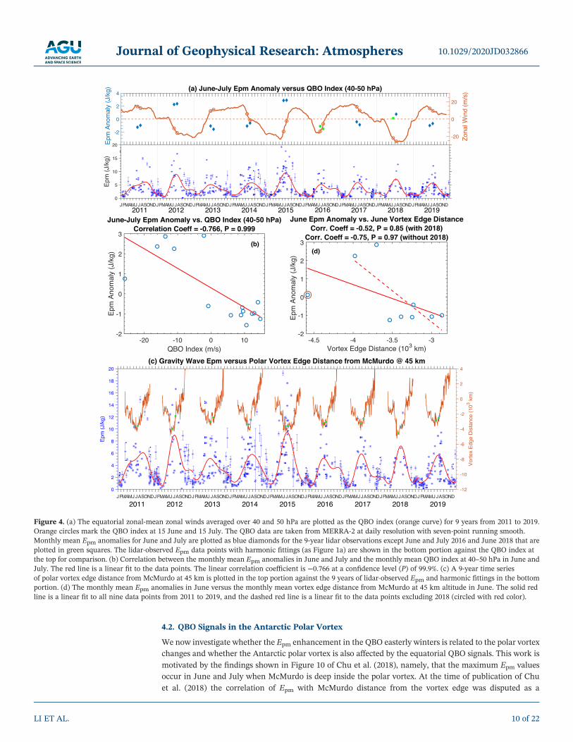
We investigate the observed interannual variations of winter Epm forpossible signatures of the QBO. A QBO index, defined as theMERRA‐2 zonal‐mean zonal winds at the equator (0° latitude) aver-aged over the 40 and 50 hPa pressure levels, is plotted versus the 9 yearsof lidar‐observed Epm data and harmonic fittings in Figure 4a.According to this QBO index, 2012, 2015, and 2018 midwinters are clas-sified as QBOe, while 2011, 2013, 2014, 2017, and 2019 are classified asQBOw. The year 2016 is abnormal as stated above—although the QBOindex at 40–50 hPa is negative, the majority of pressure levels classifythe 2016 southern winter into the westerly phase (positive index). TheAntarctic winters of 2012 and 2015 both occur in the QBO easterlyphase and correspond to high Epm peaks. Although the winter

Figure 2. Altitude mean N2 from 30 to 50 km through 9 years, 2011–2019. Each blue asterisk denotes a singleobservational segment with error bar. The red lines are (a) single‐year “annual + semiannual” fits for nine individualyears, and (b) uniform “annual + semiannual” fits for all years.

Figure 3. Nine‐year composite‐mean annual cycles of (a) Epm, (b) Epv, and(c) N2. Data are binned every 5 days at McMurdo. The red lines are theharmonic fits given by Equation 4.

10.1029/2020JD032866Journal of Geophysical Research: Atmospheres

LI ET AL. 8 of 22

maximum in 2018 is not as high as the maxima in 2012 and 2015, likely due to the lack of lidar data in June2018, it is still larger than the surrounding years like 2016, 2017, and 2019. The overall mean Epm in June andJuly over three QBOe years (2012, 2015, and 2018) are ~43% higher than the overall mean during the QBOwyears (the other six years), as computed in section 3. This Epm interannual variation has a period of roughly3 years, rather than the 28 month quasi‐biennial period (Baldwin et al., 2001). A wavelet analysis of the QBOindex at 25 hPa in Lu et al. (2019) shows that the QBO period has evolved from ~24 to ~36 months between2003 and 2018, which is consistent with the longer QBO period in the last decade of lidar observations.

To quantify the correlation between the gravity wave Epm and QBO index, we compute the Epm anomaly,wherein seasonal variations are removed. We use the harmonic fittings of nine individual years to representthe yearly Epm values and the composite‐mean fit in Figure 3a as the mean annual cycle of Epm and thensubtract the mean annual cycle from the nine individual harmonic fittings to derive the Epm anomalies.The derived Epm anomalies of two winter months (June and July) are plotted as diamonds in Figure 4a,except for 2016 and June 2018 that are plotted as squares. These results show that the positive/negativeanomalies align well with the negative/positive QBO index (easterly/westerly zonal winds at the equator),except during the abnormal year 2016. All positive Epm anomalies occur in the three QBO easterly years(2012, 2015, and 2018). In Figure 4b we plot the monthly mean Epm anomalies versus the monthly meanQBO index for June and July. Because 2016 is an abnormal year and 2018 lacks June data, Figure 4b excludes2016 data and 2018 June data. Based on the remaining 15 data points, the linear correlation coefficientbetween the Epm anomaly and the QBO index at 40–50 hPa is −0.766 with a confidence level of 99.9%.This statistically significant correlation between the gravity wave Epm and QBO phase supports that the stra-tospheric gravity wave activity is stronger in the QBO easterly winters than in the westerly winters, at leastduring the last decade. The observed interannual variations of Epm are likely due to the modulation by theQBO signals.

Table 5Harmonic Fitting Parameters and Errors for Epv in Figures 1 and 3

Case A0 (×10−2 J/m3) A12 (×10

−2 J/m3) φ12 (day) A6 (×10−2 J/m3) φ6 (day)

Figure 1c (2011) 1.19 ± 0.10 0.44 ± 0.14 234 ± 17 0.45 ± 0.13 93 ± 9Figure 1c (2012) 1.21 ± 0.10 0.66 ± 0.14 195 ± 14 0.49 ± 0.14 163 ± 9Figure 1c (2013) 0.97 ± 0.07 0.25 ± 0.09 184 ± 25 0.15 ± 0.10 136 ± 20Figure 1c (2014) 0.95 ± 0.07 0.41 ± 0.11 230 ± 13 0.02 ± 0.10 116 ± 132Figure 1c (2015) 1.20 ± 0.11 0.96 ± 0.15 194 ± 10 0.16 ± 0.15 178 ± 30Figure 1c (2016) 1.07 ± 0.08 0.51 ± 0.12 256 ± 12 0.29 ± 0.10 140 ± 10Figure 1c (2017) 0.82 ± 0.07 0.45 ± 0.08 193 ± 15 0.22 ± 0.11 162 ± 12Figure 1c (2018) 0.87 ± 0.07 0.47 ± 0.01 211 ± 11 0.30 ± 0.09 209 ± 10Figure 1c (2019) 0.76 ± 0.07 0.40 ± 0.09 206 ± 16 0.09 ± 0.09 203 ± 37Figure 1d (uniform) 0.99 ± 0.03 0.49 ± 0.04 207 ± 5 0.11 ± 0.04 154 ± 10Figure 3b (composite) 0.99 ± 0.04 0.51 ± 0.06 206 ± 7 0.12 ± 0.06 154 ± 14

Table 6Harmonic Fitting Parameters and Errors for N2 in Figures 2 and 3

Case A0 (×10−4 s−2) A12 (×10

−4 s−2) φ12 (day) A6 (×10−4 s−2) φ6 (day)

Figure 2a (2011) 4.70 ± 0.03 0.61 ± 0.03 157 ± 4 0.27 ± 0.04 179 ± 4Figure 2a (2012) 4.67 ± 0.02 0.49 ± 0.03 145 ± 4 0.21 ± 0.03 167 ± 4Figure 2a (2013) 4.67 ± 0.02 0.51 ± 0.03 148 ± 4 0.16 ± 0.03 171 ± 6Figure 2a (2014) 4.75 ± 0.02 0.60 ± 0.02 155 ± 3 0.14 ± 0.03 183 ± 5Figure 2a (2015) 4.67 ± 0.02 0.57 ± 0.03 161 ± 3 0.09 ± 0.03 191 ± 9Figure 2a (2016) 4.69 ± 0.02 0.54 ± 0.03 153 ± 3 0.24 ± 0.03 161 ± 3Figure 2a (2017) 4.60 ± 0.02 0.61 ± 0.03 137 ± 2 0.24 ± 0.03 164 ± 3Figure 2a (2018) 4.72 ± 0.01 0.57 ± 0.02 160 ± 2 0.17 ± 0.02 190 ± 3Figure 2a (2019) 4.73 ± 0.01 0.64 ± 0.03 154 ± 3 0.28 ± 0.04 173 ± 3Figure 2b (uniform) 4.69 ± 0.01 0.57 ± 0.01 154 ± 1 0.18 ± 0.01 175 ± 2Figure 3c (composite) 4.69 ± 0.01 0.57 ± 0.02 152 ± 2 0.18 ± 0.02 176 ± 3

10.1029/2020JD032866Journal of Geophysical Research: Atmospheres

LI ET AL. 9 of 22

4.2. QBO Signals in the Antarctic Polar Vortex

We now investigate whether the Epm enhancement in the QBO easterly winters is related to the polar vortexchanges and whether the Antarctic polar vortex is also affected by the equatorial QBO signals. This work ismotivated by the findings shown in Figure 10 of Chu et al. (2018), namely, that the maximum Epm valuesoccur in June and July when McMurdo is deep inside the polar vortex. At the time of publication of Chuet al. (2018) the correlation of Epm with McMurdo distance from the vortex edge was disputed as a

Figure 4. (a) The equatorial zonal‐mean zonal winds averaged over 40 and 50 hPa are plotted as the QBO index (orange curve) for 9 years from 2011 to 2019.Orange circles mark the QBO index at 15 June and 15 July. The QBO data are taken from MERRA‐2 at daily resolution with seven‐point running smooth.Monthly mean Epm anomalies for June and July are plotted as blue diamonds for the 9‐year lidar observations except June and July 2016 and June 2018 that areplotted in green squares. The lidar‐observed Epm data points with harmonic fittings (as Figure 1a) are shown in the bottom portion against the QBO index atthe top for comparison. (b) Correlation between the monthly mean Epm anomalies in June and July and the monthly mean QBO index at 40–50 hPa in June andJuly. The red line is a linear fit to the data points. The linear correlation coefficient is −0.766 at a confidence level (P) of 99.9%. (c) A 9‐year time seriesof polar vortex edge distance from McMurdo at 45 km is plotted in the top portion against the 9 years of lidar‐observed Epm and harmonic fittings in the bottomportion. (d) The monthly mean Epm anomalies in June versus the monthly mean vortex edge distance from McMurdo at 45 km altitude in June. The solid redline is a linear fit to all nine data points from 2011 to 2019, and the dashed red line is a linear fit to the data points excluding 2018 (circled with red color).

10.1029/2020JD032866Journal of Geophysical Research: Atmospheres

LI ET AL. 10 of 22

coincidence with the peak of Epm seasonal variations. Now in light of evidence of the QBO in the interannualvariations of Epm, it may not be a coincidence anymore. The shortest distance from McMurdo to the polarvortex edge is calculated on each day using the MERRA‐2 reanalysis data as described in section 2.3 andis termed “vortex edge distance.” Negative/positive vortex edge distances mean that McMurdo isinside/outside the polar vortex. Vortex edge distances are negative during the Antarctic winter due toMcMurdo being located deep inside the core of the vortex. The 9‐year time series of vortex edge distanceat 45 km is plotted against the time series of Epm in Figure 4c. Visual inspection of these two time seriessuggests that winters with lower Epm maxima, such as in 2013 and 2016, correspond to the shorter vortexdistances, that is, less negative values that occur when the vortex edge is closer to the McMurdo Station,while winters with high Epm maxima, such as in 2012, 2015 and 2018, correspond to the longer (morenegative) vortex edge distances when the vortex edge is farther away from McMurdo Station. Figure 4dshows the mean Epm anomaly in June versus the mean vortex edge distance in June. A linear fit gives acorrelation coefficient of −0.52 with a confidence level of 85% when all 9 years of lidar data are included.

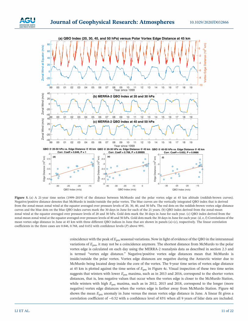
Figure 5. (a) A 21‐year time series (1999–2019) of the distance between McMurdo and the polar vortex edge at 45 km altitude (reddish‐brown curves).Negative/positive distance denotes that McMurdo is inside/outside the polar vortex. The blue curves are the vertically integrated QBO index that is derivedfrom the zonal‐mean zonal wind at the equator averaged over pressure levels of 20, 30, 40, and 50 hPa. The red dots on the reddish‐brown vortex edge distancecurves and the blue dots on the blue QBO index curves mark the 30 days in June for each of the 21 years. (b) QBO index derived from the zonal‐meanzonal wind at the equator averaged over pressure levels of 20 and 30 hPa. Gold dots mark the 30 days in June for each year. (c) QBO index derived from thezonal‐mean zonal wind at the equator averaged over pressure levels of 40 and 50 hPa. Gold dots mark the 30 days in June for each year. (d, e, f) Correlations of themean vortex edge distance in June at 45 km with three different QBO indices in June that are shown in panels (a)–(c), respectively. The linear correlationcoefficients in the three cases are 0.846, 0.768, and 0.652 with confidence levels (P) above 99%.

10.1029/2020JD032866Journal of Geophysical Research: Atmospheres

LI ET AL. 11 of 22

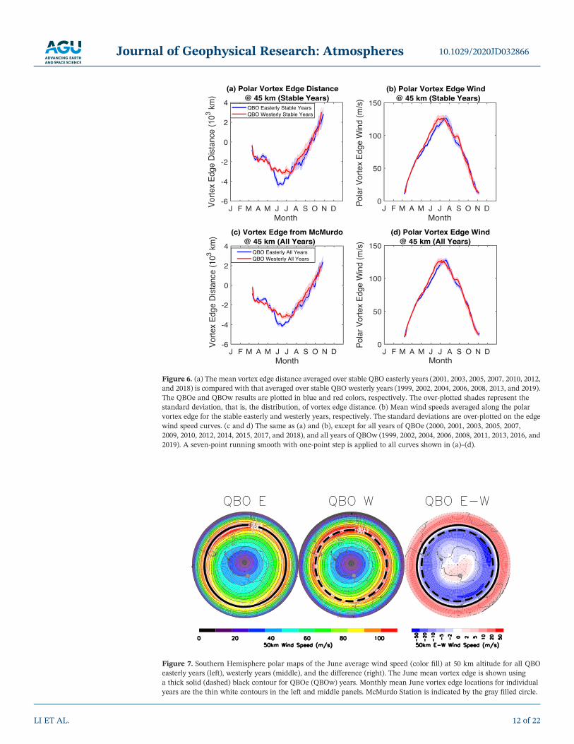
Figure 6. (a) The mean vortex edge distance averaged over stable QBO easterly years (2001, 2003, 2005, 2007, 2010, 2012,and 2018) is compared with that averaged over stable QBO westerly years (1999, 2002, 2004, 2006, 2008, 2013, and 2019).The QBOe and QBOw results are plotted in blue and red colors, respectively. The over‐plotted shades represent thestandard deviation, that is, the distribution, of vortex edge distance. (b) Mean wind speeds averaged along the polarvortex edge for the stable easterly and westerly years, respectively. The standard deviations are over‐plotted on the edgewind speed curves. (c and d) The same as (a) and (b), except for all years of QBOe (2000, 2001, 2003, 2005, 2007,2009, 2010, 2012, 2014, 2015, 2017, and 2018), and all years of QBOw (1999, 2002, 2004, 2006, 2008, 2011, 2013, 2016, and2019). A seven‐point running smooth with one‐point step is applied to all curves shown in (a)–(d).

Figure 7. Southern Hemisphere polar maps of the June average wind speed (color fill) at 50 km altitude for all QBOeasterly years (left), westerly years (middle), and the difference (right). The June mean vortex edge is shown usinga thick solid (dashed) black contour for QBOe (QBOw) years. Monthly mean June vortex edge locations for individualyears are the thin white contours in the left and middle panels. McMurdo Station is indicated by the gray filled circle.

10.1029/2020JD032866Journal of Geophysical Research: Atmospheres

LI ET AL. 12 of 22

If June 2018 data is excluded because of the lack of lidar observations in that month, then the correlationcoefficient becomes −0.75 with a confidence level of 96.7%. Figure 4d indicates that with or without June2018 data the negative correlation between Epm anomalies and polar vortex edge distances is clear. TheJune 2018 fitting data is likely an outlier, which was very likely biased toward smaller values due to thelack of observational data at a time when Epm is usually the highest. While a longer data record is needed,Figures 4c and 4d indicate a possible QBO signal in the polar vortex edge location and a correlationbetween the Epm anomaly and the vortex edge distance.

To further investigate the QBO signals in the polar vortex location, we plot the time series of 21 years(1999–2019) of vortex edge distance at 45 km in the upper portion of Figure 5a. The vortex edge distance in

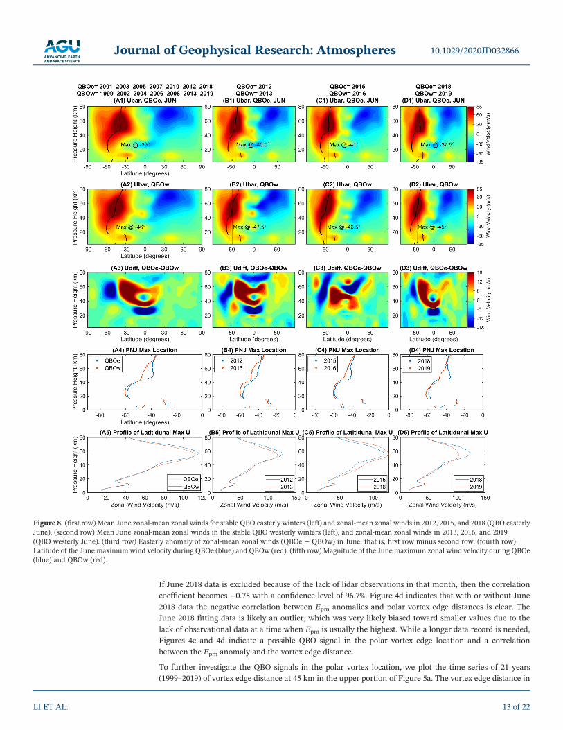
Figure 8. (first row) Mean June zonal‐mean zonal winds for stable QBO easterly winters (left) and zonal‐mean zonal winds in 2012, 2015, and 2018 (QBO easterlyJune). (second row) Mean June zonal‐mean zonal winds in the stable QBO westerly winters (left), and zonal‐mean zonal winds in 2013, 2016, and 2019(QBO westerly June). (third row) Easterly anomaly of zonal‐mean zonal winds (QBOe − QBOw) in June, that is, first row minus second row. (fourth row)Latitude of the June maximum wind velocity during QBOe (blue) and QBOw (red). (fifth row) Magnitude of the June maximum zonal wind velocity during QBOe(blue) and QBOw (red).

10.1029/2020JD032866Journal of Geophysical Research: Atmospheres

LI ET AL. 13 of 22

June (red color) is farther (more negative edge distances) in the QBOe (negative QBO winds) and closer (lessnegative edge distances) in the QBOw (positive QBO winds). Three different QBO indices are shown in thebottom portion of Figures 5a–5c. The new QBO index in Figure 5a is defined as the zonal‐mean zonal windat the equator averaged over pressure levels of 20, 30, 40, and 50 hPa, while the QBO indices in Figures 5b and5c are the zonal winds averaged over pressure levels of 20 and 30 hPa and over pressure levels of 40 and50 hPa, respectively. Asmentioned earlier, different QBO indices defined at different pressure levels can alterthe QBO easterly and westerly classifications for some June months. For example, 2000, 2009, 2011, 2014,2015, 2016, and 2017 flip signs between the 20–30 hPa QBO index of Figure 5b and the 40–50 hPa QBO indexof Figure 5c. At the same time, 2001, 2003, 2005, 2007, 2010, 2012, and 2018 remain in theQBO easterly phase,while 1999, 2002, 2004, 2006, 2008, 2013, and 2019 remain in the QBO westerly phase under all three QBOindices. The monthly means of vortex edge distance in June at 45 km altitude are plotted against the Junemeans of three different QBO indices in Figures 5d–5f, respectively. All three figures show positive correla-tions between the vortex edge distance and the QBO indices, that is, more negative vortex edge distances(McMurdo is inside and farther from the vortex edge) correspond to more negative (easterly) QBO winds.Likewise, less negative vortex edge distances (McMurdo is inside but closer to the vortex edge) correspondto more positive (westerly) QBO winds. The linear correlation coefficients are 0.846, 0.768, and 0.652 withconfidence levels of 100%, 99.995%, and 99.863%, respectively. Over this 21‐year period, the QBO signals inthe polar vortex edge location are robust and have statistical significance. The new QBO index givenin Figure 5a has the highest correlation with the vortex edge distance. This new index is the integration(i.e., the mean) of all four pressure levels of 20, 30, 40, and 50 hPa, reflecting the downward progression ofthe equatorial zonal wind better than other two indices. This analysis convincingly shows that the polar vor-tex edge moves equatorward in the QBO easterly winters and moves poleward in the QBO westerly winters.

Winters (June) with consistent easterly (2001, 2003, 2005, 2007, 2010, 2012, and 2018) or westerly (1999,2002, 2004, 2006, 2008, 2013, and 2019) classifications (they do not flip signs for different QBO indices)are termed the “stable years” (stable winters) of QBOe or QBOw, while the rest (2000, 2009, 2011, 2014,2015, 2016, and 2017) are called “transition years.” The set including both stable and transition years isreferred to as the “all years” set. Using the vertically integrated QBO index given in Figure 5a, we classifythe “all years” set of QBO easterly winters as (2000, 2001, 2003, 2005, 2007, 2009, 2010, 2012, 2014, 2015,2017, and 2018) and the “all years” set of QBO westerly winters as (1999, 2002, 2004, 2006, 2008, 2011,2013, 2016, and 2019). We now average the vortex edge distance and mean wind speed along the vortex edgewithin these two groups. Two trials are made—one averages over the stable years of QBOe and QBOw, andanother averages over the “all years” sets for QBOe and QBOw. The “stable years” results are compared inFigures 6a and 6b, and the “all years” results are in Figures 6c and 6d for the vortex edge at 45 km altitude. Itis clear in both cases that the polar vortex edge stays farther away from McMurdo in the QBO easterly yearsthan in the westerly years during the midwinter, and the differences in vortex edge distance reach the max-imum in June with a time span of about 2 months (frommid‐May to mid‐July). The differences in the meansof the stable winters (about 1,200 km) are larger than those in the means of “all years” winters (about900 km), as expected. The differences in the mean winds along the vortex edge are relatively small, but ingeneral the mean winds in the QBOe are weaker than in the QBOw by about 10–20 m/s in June. Note thatthe QBO differences seen in vortex edge distance and vortex edge wind speed are seasonally dependent.

To further investigate the polar vortex changes, three panels of polar vortex maps in the SouthernHemisphere (SH) are plotted in Figure 7. All panels are derived from MERRA‐2 reanalysis data from 1999to 2019 for June near 50 km altitude. The left panel shows the average June wind speed (in color) andAntarctic vortex edge (thick black contour) for QBO easterly years. The thin white contours are the vortexedge for the individual easterly years. Themiddle panel is the June average for QBOwesterly years. The rightpanel is the difference (QBOe − QBOw) in wind speed (blue/red colors) and the mean vortex edge for east-erly years (solid black) and for westerly years (dashed black). This right panel shows that the zonal wind overMcMurdo (marked by a gray filled circle) is ~5–10 m/s faster in the QBOe than in the QBOw at 50 km. Theblue shades from 40–70°S latitudes and the red shades equatorward of 40°S in the right panel of Figure 7reflect an equatorward shift in the PNJ during QBO easterly years. In terms of the vortex edge, the Junemean vortex edge is located at 39.7°S latitude during QBO easterly years and at 47.7°S latitude duringQBO westerly years (right panel) when all years of QBOe and QBOw are included. Removing two suddenstratospheric warming (SSW) years (2002 and 2019) from QBOw, the mean vortex edge in June is located

10.1029/2020JD032866Journal of Geophysical Research: Atmospheres

LI ET AL. 14 of 22

at 39.7°S and 47.2°S for QBOe and QBOw, respectively, making only a 6% difference. The difference of7.5–8°S latitude between the QBOe and QBOw years is statistically significant and it confirms that theQBO signals in the vortex edge distance shown in Figures 5 and 6 are robust.

5. Interannual Variations of PNJ in June and Critical Level Filtering Effects5.1. Equatorward Shift of the SH PNJ in June During QBOe

Our results indicate that the QBO signals in the Antarctic polar vortex edge location are largest in June. Thisfinding prompts us to examine the PNJ in June in order to understand the environment surrounding thepolar vortex. We average the MERRA‐2 zonal‐mean zonal winds (U‐bar) over the stable years of QBOeand QBOw, respectively, for June in Figures 8a1 and 8a2, and take the differences between them inFigure 8a3. This differentiation method is similar to that of Baldwin and Dunkerton (1998), Hitchmanand Huesmann (2009), and Lu et al. (2019). As MERRA‐2 is a pressure level‐based model, the data are con-verted to pressure heights (z) using the equation z ¼ H · log(po/p), where the scale height (H) is set to 7 kmand po ¼ 1,000 hPa. On these plots, the PNJ core is defined as the maximum zonal wind velocity (eastward)in the latitude‐altitude plane and is overlaid for each altitude on Figures 8a1 and 8a2, as well as its locationreiterated and value displayed in Figures 8a4 and 8a5, respectively.

From the Figures 8a1 and 8a2, we can see that the maximum U‐bar occurs around 50 km altitude at −39°and−46° latitude for the QBOe and QBOw, respectively, showing that the PNJ core location moves equator-ward in a QBO easterly phase as compared to a QBO westerly phase by ~7° latitude. Figure 8a3 displays thedifferent responses of different regions to the changing QBO phase. Figure 8a4 shows that the maximumwind location varies with altitude, reaching equatorwardmost near the stratopause and lower mesosphere(~45–60 km) and slowly moving poleward with decreasing altitude to around−60° latitude in the lower stra-tosphere (~20–30 km). The equatorward shift during QBOe can again be seen here, but no major differencescan be discerned in zonal wind velocity for any altitude between QBO phases in Figure 8a5. The shift in PNJlocation seen in Figures 8a1–8a4 is a clear reflection of the vortex expansion during QBOe demonstratedabove. During the QBO easterly phase, the polar vortex expands, pushing the PNJ toward the equator. Itis worth mentioning that Yamashita et al. (2018) reported a seemingly opposite result in July that theQBO westerly phase corresponds to an equatorward vortex shift. However, further examination shows thata QBO index defined at 10–20 hPa in Yamashita et al. (2018) is almost opposite to the QBO phase classifica-tions shown in our Figure 5a. Therefore, their results are basically consistent with our findings in June.

The easterly anomalies (QBOe − QBOw) in Figure 8a3 show a triple‐cell structure from the equator to theSouth Pole around the stratopause. The June zonal‐mean zonal winds in the QBOe are stronger in the equa-torial to subtropical region (0–40°S), weaker in the midlatitude to high‐latitude region (45–70°S), andslightly stronger in the polar region (75–90°S) than those in the QBOw between 40 and 70 km altitude.Such pattern around the stratopause is similar to the dipole‐cell structure poleward of 30°S in Augustreported by Lu et al. (2019). This pattern also supports a finding of the northern‐southern hemispheric asym-metry in the QBO easterly anomalies of zonal‐mean zonal winds in Lu et al. (2019). The NorthernHemisphere QBO easterly anomalies in Figure 2 (D3) of Lu et al. (2019) reveal a two‐cell structure fromthe equator to the North Pole around the stratopause in January, in contrast to the triple‐cell structureshown here. Our tests have revealed that this triple‐cell pattern around the stratopause is robust in June,insensitive to including or removing years from the data set. Figure 8a3 shows negligible differences betweenQBOe and QBOw below 30 km in the polar region in June, which agrees with the August result of Baldwinand Dunkerton (1998). Columns 2–4 of Figure 8 are included to demonstrate that variability exists betweenyears, but the QBO phase‐related behavior is still well represented by the “stable” years used in Column 1.The three displayed QBO easterly winters (2012, 2015, and 2018) have higher June and July Epm values thanother years and correspond to the equatorward shifted PNJ as compared to the adjacent QBO westerly win-ters (2013, 2016, and 2019). It can also be seen that the trends demonstrated in each row of plots are similarfrom column to column.

5.2. Effects of Critical Level Filtering on Gravity Wave Epm

Why does an equatorward expanding vortex (in QBOe) correspond to enhanced Epm? There may be severalfactors contributing to this correlation with critical level filtering as one of the major factors. The expanding

10.1029/2020JD032866Journal of Geophysical Research: Atmospheres

LI ET AL. 15 of 22

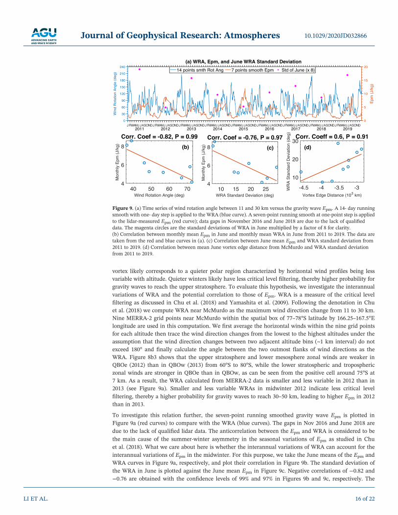
vortex likely corresponds to a quieter polar region characterized by horizontal wind profiles being lessvariable with altitude. Quieter winters likely have less critical level filtering, thereby higher probability forgravity waves to reach the upper stratosphere. To evaluate this hypothesis, we investigate the interannualvariations of WRA and the potential correlation to those of Epm. WRA is a measure of the critical levelfiltering as discussed in Chu et al. (2018) and Yamashita et al. (2009). Following the denotation in Chuet al. (2018) we compute WRA near McMurdo as the maximum wind direction change from 11 to 30 km.Nine MERRA‐2 grid points near McMurdo within the spatial box of 77–78°S latitude by 166.25–167.5°Elongitude are used in this computation. We first average the horizontal winds within the nine grid pointsfor each altitude then trace the wind direction changes from the lowest to the highest altitudes under theassumption that the wind direction changes between two adjacent altitude bins (~1 km interval) do notexceed 180° and finally calculate the angle between the two outmost flanks of wind directions as theWRA. Figure 8b3 shows that the upper stratosphere and lower mesosphere zonal winds are weaker inQBOe (2012) than in QBOw (2013) from 60°S to 80°S, while the lower stratospheric and troposphericzonal winds are stronger in QBOe than in QBOw, as can be seen from the positive cell around 75°S at7 km. As a result, the WRA calculated from MERRA‐2 data is smaller and less variable in 2012 than in2013 (see Figure 9a). Smaller and less variable WRAs in midwinter 2012 indicate less critical levelfiltering, thereby a higher probability for gravity waves to reach 30–50 km, leading to higher Epm in 2012than in 2013.

To investigate this relation further, the seven‐point running smoothed gravity wave Epm is plotted inFigure 9a (red curves) to compare with the WRA (blue curves). The gaps in Nov 2016 and June 2018 aredue to the lack of qualified lidar data. The anticorrelation between the Epm and WRA is considered to bethe main cause of the summer‐winter asymmetry in the seasonal variations of Epm as studied in Chuet al. (2018). What we care about here is whether the interannual variations of WRA can account for theinterannual variations of Epm in the midwinter. For this purpose, we take the June means of the Epm andWRA curves in Figure 9a, respectively, and plot their correlation in Figure 9b. The standard deviation ofthe WRA in June is plotted against the June mean Epm in Figure 9c. Negative correlations of −0.82 and−0.76 are obtained with the confidence levels of 99% and 97% in Figures 9b and 9c, respectively. The

Figure 9. (a) Time series of wind rotation angle between 11 and 30 km versus the gravity wave Epm. A 14‐ day runningsmooth with one‐ day step is applied to the WRA (blue curve). A seven‐point running smooth at one‐point step is appliedto the lidar‐measured Epm (red curve); data gaps in November 2016 and June 2018 are due to the lack of qualifieddata. The magenta circles are the standard deviations of WRA in June multiplied by a factor of 8 for clarity.(b) Correlation between monthly mean Epm in June and monthly mean WRA in June from 2011 to 2019. The data aretaken from the red and blue curves in (a). (c) Correlation between June mean Epm and WRA standard deviation from2011 to 2019. (d) Correlation between mean June vortex edge distance from McMurdo and WRA standard deviationfrom 2011 to 2019.

10.1029/2020JD032866Journal of Geophysical Research: Atmospheres

LI ET AL. 16 of 22

standard deviation of WRA is used here to represent the stability of the background winds, which may beaffected by the relative location between McMurdo and the vortex edge. When the polar vortex edge movesequatorward, thusMcMurdo being well inside the polar vortex, the backgroundwinds are likely more stable,thereby lower standard deviation ofWRA and less critical level filtering are expected. Plotting theWRA stan-dard deviation in June against the vortex edge distance in June in Figure 9d, we do see a positive correlationof ~0.6, although the confidence level (91%) is less than 95%. The results above support the hypothesis thatthe interannual variations of Epm is mainly determined by the interannual variations ofWRA that is stronglyinfluenced by the polar vortex location in the midwinter. The equatorward expansion of the polar vortex inthe QBO easterly phase leads to quieter winters and more stable background winds that correspond to lesscritical level filtering and thus higher Epm in the upper stratosphere. Lidar observations in Alaska also showsignificant interannual variations in gravity wave Epm averaged over three winter months (December,January, and February) from 40 to 50 km (Triplett et al., 2017). The highest gravity wave activity occurredduring quiet winters when no SSW occurred, and the lowest gravity wave activity in the disturbed winterswhen major SSWs occurred (Triplett et al., 2017). These Arctic results are basically consistent with our find-ings of higher Epm occurring in quieter Antarctic winters (QBOe).

6. Discussion

There are additional long‐term variations that affect the polar wind and temperature fields, thus influencingthe interannual variations of gravity waves and polar vortex. Here we briefly discuss two major factors—thesolar cycle and the El Niño–Southern Oscillation (ENSO). The Holton‐Tan effect, based on the NorthernHemisphere studies (Holton & Tan, 1988), emphasizes that the effective waveguide for upward and equator-ward propagating planetary‐scale waves is altered by the tropical winds. The zonal wind structure in theQBO easterly phase focuses more wave activity toward the pole, where planetary waves converge and slowdown the zonal‐mean flow. Hence, the Arctic polar winter vortex tends to be disturbed and weak when theQBO is easterly but undisturbed and strong when the QBO is westerly. Baldwin et al. (2001) point out thatthe QBO acts as predicted by Holton and Tan (1980) only in years with low solar activity but appears toreverse its behavior during years with high solar activity (Labitzke, 1987; Labitzke & van Loon, 1988; vanLoon & Labitzke, 1994). Given the interhemispheric asymmetry in the QBO easterly anomalies (section 5.1),it is necessary to examine the response of QBO signals to solar activity in the SH. Analyzing the 21‐year timeseries in Figure 5a, 1999–2003 corresponds to a solar maximum, while 2006–2011 corresponds to a solarminimum; however, the equatorward shift of the SH polar vortex in the QBOe occurs during both the solarmaximum and minimum periods. To the first order, the robust QBO signals in the latitudes of vortex edgeand PNJ are not affected by solar activity.

ENSO has been shown to affect the latitude of the June PNJ (Yamashita et al., 2018). The ENSO indexused in that work was calculated from the 5 month running mean data of the Nino 3.4 index (NINO3.4)(http://www.esrl.noaa.gov/psd/data/correlation/nina34.data) provided by the National Oceanic andAtmospheric Administration (NOAA)/Earth System Research Laboratory. We find no correlation betweenthe ENSO index and the vortex edge distance from 1999 to 2019 or from 1980 to 2019. Even after separatingthe vortex edge distance data into the QBOe and QBOw phases, there is still no statistically significant cor-relation. Therefore, the QBO signals in the vortex edge location and the latitude of the PNJ are robust and arenot attributed to ENSO. Investigating the relationship between the ENSO index and the lidar‐observed Epm,we note a possible link between a particularly strong ENSO year and the year of our highest Epm measure-ment (2015). However, there is no individual year correlation between ENSO and Epm in the last decade. Forexample, 2019 corresponds to the second highest ENSO index among the nine years of 2011–2019 but one ofthe lowest Epm winter maxima, while 2012 and 2018 correspond to the second and third highest Epm, but theENSO indices in these two years are lower than that in 2019. Therefore, it is most likely that the interannualvariations of the gravity wave Epm are mainly controlled by the QBO signals, not the ENSO effects, althoughthe possible influence of ENSO on the highest Epm year is noticeable and a longer data record is needed todraw definitive conclusions.

The benefit of using a longer data record can be demonstrated in the following student t tests. From the sta-tistics point of view, the linear correlations obtained in Figures 4b, 4d, 5d–5f, and 9b–9d are the sample

10.1029/2020JD032866Journal of Geophysical Research: Atmospheres

LI ET AL. 17 of 22

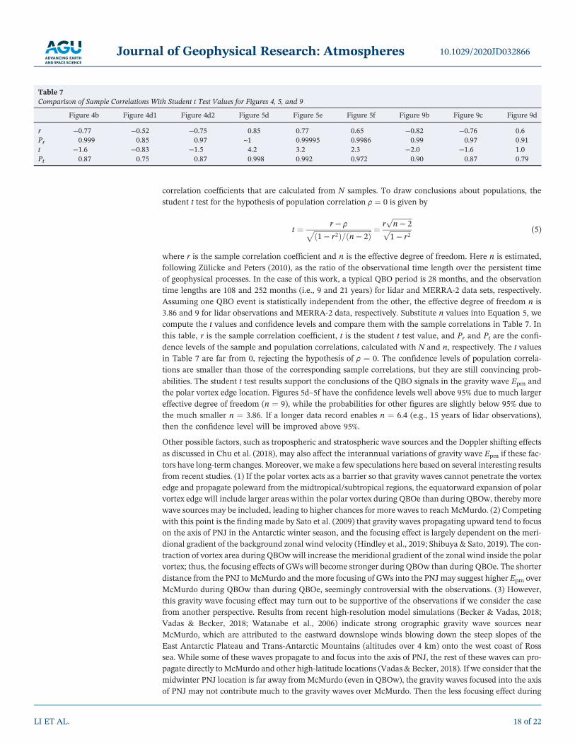
correlation coefficients that are calculated from N samples. To draw conclusions about populations, thestudent t test for the hypothesis of population correlation ρ ¼ 0 is given by

t ¼ r − ρffiffiffiffiffiffiffiffiffiffiffiffiffiffiffiffiffiffiffiffiffiffiffiffiffiffiffiffiffiffiffiffiffi1 − r2ð Þ= n − 2ð Þp ¼ r

ffiffiffiffiffiffiffiffiffiffiffin − 2

pffiffiffiffiffiffiffiffiffiffiffiffi1 − r2

p (5)

where r is the sample correlation coefficient and n is the effective degree of freedom. Here n is estimated,following Zülicke and Peters (2010), as the ratio of the observational time length over the persistent timeof geophysical processes. In the case of this work, a typical QBO period is 28 months, and the observationtime lengths are 108 and 252 months (i.e., 9 and 21 years) for lidar and MERRA‐2 data sets, respectively.Assuming one QBO event is statistically independent from the other, the effective degree of freedom n is3.86 and 9 for lidar observations and MERRA‐2 data, respectively. Substitute n values into Equation 5, wecompute the t values and confidence levels and compare them with the sample correlations in Table 7. Inthis table, r is the sample correlation coefficient, t is the student t test value, and Pr and Pt are the confi-dence levels of the sample and population correlations, calculated with N and n, respectively. The t valuesin Table 7 are far from 0, rejecting the hypothesis of ρ ¼ 0. The confidence levels of population correla-tions are smaller than those of the corresponding sample correlations, but they are still convincing prob-abilities. The student t test results support the conclusions of the QBO signals in the gravity wave Epm andthe polar vortex edge location. Figures 5d–5f have the confidence levels well above 95% due to much largereffective degree of freedom (n ¼ 9), while the probabilities for other figures are slightly below 95% due tothe much smaller n ¼ 3.86. If a longer data record enables n ¼ 6.4 (e.g., 15 years of lidar observations),then the confidence level will be improved above 95%.

Other possible factors, such as tropospheric and stratospheric wave sources and the Doppler shifting effectsas discussed in Chu et al. (2018), may also affect the interannual variations of gravity wave Epm if these fac-tors have long‐term changes. Moreover, we make a few speculations here based on several interesting resultsfrom recent studies. (1) If the polar vortex acts as a barrier so that gravity waves cannot penetrate the vortexedge and propagate poleward from the midtropical/subtropical regions, the equatorward expansion of polarvortex edge will include larger areas within the polar vortex during QBOe than during QBOw, thereby morewave sources may be included, leading to higher chances for more waves to reach McMurdo. (2) Competingwith this point is the finding made by Sato et al. (2009) that gravity waves propagating upward tend to focuson the axis of PNJ in the Antarctic winter season, and the focusing effect is largely dependent on the meri-dional gradient of the background zonal wind velocity (Hindley et al., 2019; Shibuya & Sato, 2019). The con-traction of vortex area during QBOwwill increase the meridional gradient of the zonal wind inside the polarvortex; thus, the focusing effects of GWs will become stronger during QBOw than during QBOe. The shorterdistance from the PNJ to McMurdo and the more focusing of GWs into the PNJ may suggest higher Epm overMcMurdo during QBOw than during QBOe, seemingly controversial with the observations. (3) However,this gravity wave focusing effect may turn out to be supportive of the observations if we consider the casefrom another perspective. Results from recent high‐resolution model simulations (Becker & Vadas, 2018;Vadas & Becker, 2018; Watanabe et al., 2006) indicate strong orographic gravity wave sources nearMcMurdo, which are attributed to the eastward downslope winds blowing down the steep slopes of theEast Antarctic Plateau and Trans‐Antarctic Mountains (altitudes over 4 km) onto the west coast of Rosssea. While some of these waves propagate to and focus into the axis of PNJ, the rest of these waves can pro-pagate directly to McMurdo and other high‐latitude locations (Vadas & Becker, 2018). If we consider that themidwinter PNJ location is far away from McMurdo (even in QBOw), the gravity waves focused into the axisof PNJ may not contribute much to the gravity waves over McMurdo. Then the less focusing effect during

Table 7Comparison of Sample Correlations With Student t Test Values for Figures 4, 5, and 9

Figure 4b Figure 4d1 Figure 4d2 Figure 5d Figure 5e Figure 5f Figure 9b Figure 9c Figure 9d

r −0.77 −0.52 −0.75 0.85 0.77 0.65 −0.82 −0.76 0.6Pr 0.999 0.85 0.97 ~1 0.99995 0.9986 0.99 0.97 0.91t −1.6 −0.83 −1.5 4.2 3.2 2.3 −2.0 −1.6 1.0Pt 0.87 0.75 0.87 0.998 0.992 0.972 0.90 0.87 0.79

10.1029/2020JD032866Journal of Geophysical Research: Atmospheres

LI ET AL. 18 of 22

QBOe means more chance for gravity waves to propagate to McMurdo from wave sources and thus possiblyhigher Epm during QBOe as the lidar observed. Quantitative analyses of these factors, including the solarcycle and ENSO effects, and their contributions to the enhanced Epm in the QBO easterly phase are beyondthe scope of this work but will be addressed in future modeling studies.

7. Conclusions

Using 9 years of lidar observations (2011–2019) from McMurdo/Arrival Heights (77.84°S, 166.67°E),Antarctica, and 21 years of MERRA‐2 reanalysis data (1999–2019), we present the first observations of poten-tial QBO signals in the stratospheric gravity wave potential energy mass density (Epm) at McMurdo and inthe Antarctic polar vortex location near the stratopause. Midwinter stratospheric gravity wave activity isstronger during the QBO easterly years when the June polar vortex expands and the PNJ shifts equatorward.During the QBO westerly years, gravity wave activity is weaker when the polar vortex contracts and the PNJmoves poleward. The lidar‐observed interannual variations of gravity wave Epm winter maxima overMcMurdo are most likely controlled by the equatorial QBO signals via modulating the polar vortex locationand thus the critical level filtering of gravity waves in the Antarctic. The ENSO may play a minor role inmodulating the Epm interannual variations. The QBO signals in the polar vortex edge and PNJ duringJune months are robust and appear not to be affected by the solar cycle and ENSO to the first order.

In addition to the repeated seasonal pattern of summer minima and winter maxima, qualified lidar data of~7,000 hr also exhibit interannual variations of gravity wave Epm in the stratosphere 30–50 km. That is, themean Epm winter maxima in 2012, 2015, and 2018 (during QBOe) are ~43% higher than those in the otheryears (during QBOw). Using the 9‐year composite‐mean harmonic fit to represent the mean annual cycle,the McMurdo lidar observations reveal the positive/negative gravity wave Epm anomalies during QBOeasterly/westerly winters. The correlation of the Epm anomaly with a QBO index averaged over the 40 and50 hPa pressure levels reaches a coefficient of −0.766 with a confidence level of 99.9%, confirming a statis-tically significant correlation between the gravity wave Epm and the QBO phase in the last decade. The posi-tive Epm anomalies occur when McMurdo is well inside the polar vortex core and the distance to the vortexedge is large; both of these aspects tend to occur during the QBO easterly winters.

Using the 21 years of MERRA‐2 reanalysis data (1999–2019), we find that the June polar vortex edge near thestratopause moves equatorward/poleward during QBO easterly/westerly years. The correlation between thenegative vortex edge distance from McMurdo at 45 km and a QBO index vertically averaged over 20, 30, 40,and 50 hPa pressure levels reaches a correlation coefficient of 0.846 with a confidence level of nearly 100%.The mean distance from McMurdo to the vortex edge, averaged over the QBO easterly years, reaches over4,000 km, while the distance averaged over the QBO westerly years is about 3,000 km in June at 45 km.The mean wind along the vortex edge in June is weaker by 10–20 m/s in the QBO easterly than in the wes-terly years. Such vortex edge distance corresponds to the mean vortex edge near the stratopause (~50 km)located at 39.7°S and 47.7°S, respectively, for the QBO easterly and westerly phases. This latitude differenceof ~8° is significant as it equates to a distance of nearly 1,000 km. The QBO signal in the polar vortex edgelocation is robust with statistical significance.

The equatorward shift of the PNJ core around the stratopause in the QBO easterly years and the polewardshift in the QBO westerly years are clear reflections of the vortex expansion/contraction during QBOeasterly/westerly phases. The polar vortex edge is located along the poleward flank of the PNJ stream.During the QBO easterly phase, the polar vortex expands, pushing the PNJ toward the equator. The equator-ward expansion of the polar vortex leads to quieter winters and more stable background winds during QBOethan QBOw and corresponds to less critical level filtering and thus higher Epm in the upper stratosphere inthe QBO easterly phase. The critical level filtering is characterized by the WRA, and our results support thehypothesis that the interannual variations of Epm is mainly determined by the interannual variations ofWRA, that is, the critical level filtering effects. WRA is likely modulated by the polar vortex location inthe midwinter.

Why the SH polar vortex moves equatorward in QBOe, why the triple‐cell structures are formed around thestratopause in the SH, and why gravity wave Epm at McMurdo are enhanced in the QBOe when the polarvortex and PNJ move equatorward, are beyond the scope of this study. These intriguing questions deserve

10.1029/2020JD032866Journal of Geophysical Research: Atmospheres

LI ET AL. 19 of 22

future investigations with the combination of theories, models, and long‐term observations. The underlyingmechanisms may well reflect the asymmetry between two hemispheres and the complex atmospheric cou-pling from the equatorial to the polar regions. Furthermore, the QBO modulation of stratospheric gravitywaves may impact the vertical wave coupling via modulating the generation of secondary gravity waves(Vadas et al., 2018) and wave dissipation altitudes (Vadas & Becker, 2019), which will affect persistent grav-ity waves in theMLT (Chen et al., 2016; Chu et al., 2018). It is likely to findQBO signals in theMLT, and suchquestions deserve future investigation using the lidar data collected from McMurdo. The observationallybased study presented in this article lays the groundwork for future modeling studies that will test theobserved relationships and proposed mechanisms in long‐term climate simulations. Other future work willalso investigate the roles of solar activity and ENSO as well as their entanglement with the QBO, polar vor-tex, and gravity waves.

Data Availability Statement

The data shown in this work can be downloaded online (from https://data.mendeley.com/datasets/96yhm3ct24/1).

ReferencesAlexander, M. J., Geller, M., McLandress, C., Polavarapu, S., Preusse, P., Sassi, F., et al. (2010). Recent developments in gravity‐wave effects

in climate models and the global distribution of gravity‐wave momentum flux from observations and models. Quarterly Journal of theRoyal Meteorological Society, 136(650), 1103–1124. https://doi.org/10.1002/qj.637

Andrews, D. G., Holton, J. R., & Leovy, C. B. (1987). Middle atmosphere dynamics (). New York: Elsevier.Anstey, J. A., & Shepherd, T. G. (2014). High‐latitude influence of the Quasi‐Biennial Oscillation. Quarterly Journal of the Royal

Meteorological Society, 140(678), 1–21. https://doi.org/10.1002/qj.2132Baldwin, M. P., & Dunkerton, T. J. (1998). Quasi‐biennial modulation of the Southern Hemisphere stratospheric polar vortex. Geophysical

Research Letters, 25(17), 3343–3346. https://doi.org/10.1029/98GL02445Baldwin, M. P., Gray, L. J., Dunkerton, T. J., Hamilton, K., Haynes, P. H., Randel, W. J., et al. (2001). The Quasi‐Biennial Oscillation.

Reviews of Geophysics, 39(2), 179–229. https://doi.org/10.1029/1999rg000073Becker, E. (2012). Dynamical control of the middle atmosphere. Space Science Reviews, 168(1‐4), 283–314. https://doi.org/10.1007/s11214-

011-9841-5Becker, E. (2017). Mean‐flow effects of thermal tides in the mesosphere and lower thermosphere. Journal of the Atmospheric Sciences, 74(6),

2043–2063. https://doi.org/10.1175/jas-d-16-0194.1Becker, E., & Vadas, S. L. (2018). Secondary gravity waves in the winter mesosphere: Results from a high‐resolution global circulation

model. Journal of Geophysical Research: Atmospheres, 123, 2605–2627. https://doi.org/10.1002/2017jd027460Bosilovich, M. G., Akella, S., Coy, L., Cullather, R., Draper, C., Gelaro, R., et al. (2015). MERRA‐2: Initial evaluation of the ClimateRep.

Greenbelt, MD: NASA.Chen, C. (2016). Exploration of the mystery of polar wave dynamics with lidar/radar observations and general circulation models &

development of new wave analysis methods (Doctoral Ddissertation). University of Colorado, Boulder, Boulder, Colorado.Chen, C., & Chu, X. (2017). Two‐dimensional Morlet wavelet transform and its application to wave recognition methodology of

automatically extracting two‐dimensional wave packets from lidar observations in Antarctica. Journal of Atmospheric andSolar‐Terrestrial Physics, 162, 28–47. https://doi.org/10.1016/j.jastp.2016.10.016

Chen, C., Chu, X., McDonald, A. J., Vadas, S. L., Yu, Z., Fong, W., & Lu, X. (2013). Inertia‐gravity waves in Antarctica: A case study usingsimultaneous lidar and radar measurements at McMurdo/Scott Base (77.8°S, 166.7°E). Journal of Geophysical Research: Atmospheres,118, 2794–2808. https://doi.org/10.1002/jgrd.50318

Chen, C., Chu, X., Zhao, J., Roberts, B. R., Yu, Z., Fong, W., et al. (2016). Lidar observations of persistent gravity waves with periods of3–10 h in the Antarctic middle and upper atmosphere at McMurdo (77.83°S, 166.67°E). Journal of Geophysical Research: Space Physics,121, 1483–1502. https://doi.org/10.1002/2015ja022127

Chu, X., Huang,W., Fong,W., Yu, Z.,Wang, Z., Smith, J. A., &Gardner, C. S. (2011). First lidar observations of polarmesospheric clouds andFe temperatures at McMurdo (77.8°S, 166.7°E), Antarctica. Geophysical Research Letters, 38, L16810. https://doi.org/10.1029/2011GL048373

Chu, X., Pan,W., Papen, G. C., Gardner, C. S., & Gelbwachs, J. A. (2002). Fe Boltzmann temperature lidar: Design, error analysis, and initialresults at the North and South Poles. Applied Optics, 41(21), 4400–4410. https://doi.org/10.1364/AO.41.004400

Chu, X., & Yu, Z. (2017). Formation mechanisms of neutral Fe layers in the thermosphere at Antarctica studied with athermosphere‐ionosphere Fe/Fe+ (TIFe) model. Journal of Geophysical Research: Space Physics, 122, 6812–6848. https://doi.org/10.1002/2016ja023773

Chu, X., Yu, Z., Chen, C., Fong, W., Huang, W., & Gardner, C. S., et al. (2012). McMurdo lidar campaign: A new look into polar upperatmosphere. Paper presented at the 26th International Laser Radar Conference, Porto Heli, Greece.

Chu, X., Yu, Z., Fong, W., Chen, C., Zhao, J., Barry, I. F., et al. (2016). From Antarctica lidar discoveries to oasis exploration. EuropeanPhysical Journal Web of Conferences, 119, 12001. https://doi.org/10.1051/epjconf/201611912001

Chu, X., Yu, Z., Gardner, C. S., Chen, C., & Fong, W. (2011). Lidar observations of neutral Fe layers and fast gravity waves in thethermosphere (110–155 km) at McMurdo (77.8°S, 166.7°E), Antarctica. Geophysical Research Letters, 38, L23807. https://doi.org/10.1029/2011GL050016

Chu, X., Zhao, J., Lu, X., Harvey, V. L., Jones, R. M., Becker, E., et al. (2018). Lidar observations of stratospheric gravity waves from 2011 to2015 at McMurdo (77.84°S, 166.69°E), Antarctica: 2. Potential energy densities, lognormal distributions, and seasonal variations. Journalof Geophysical Research: Atmospheres, 123, 7910–7934. https://doi.org/10.1029/2017JD027386

10.1029/2020JD032866Journal of Geophysical Research: Atmospheres

LI ET AL. 20 of 22

AcknowledgmentsWe gratefully acknowledge thegraduate students and researchscientists who made contributions tothe McMurdo lidar campaign,including winter‐over lidar scientistsZhibin Yu (2011), Brendan Roberts(2012), Weichun Fong (2013), CaoChen (2014), Jian Zhao (2015), IanBarry (2016), Zhengyu Hua (2017),Dongming Chang (2018), Zimu Li andIan Geraghty (2019), Xianxin Li andCissi Lin (2020), and summer scientistsWentao Huang, Zhangjun Wang, JohnA. Smith, Xian Lu, Muzhou Lu, ClareMiller, and Jackson Jandreau. We aregrateful to Richard Dean, NikolasSinkola, Adam Godfrey, Mark Murphy,Hue Tran, and Kate McKenzie for theirengineering help and support. Wethank Erich Becker and Sharon L.Vadas for intriguing discussions onorographic gravity waves and criticallevel filtering. We are indebted toVladimir Papitashvili, Chester S.Gardner, and Adrian J. McDonald fortheir guidance and collaboration. Wesincerely appreciate the staff of theUnited States Antarctic Program,McMurdo Station, Antarctica, NewZealand, and Scott Base for their superbsupport over the years. We gratefullyacknowledge MERRA‐2 data providedby the Global Modeling andAssimilation Office (GMAO) at NASAGoddard Space Flight Center throughthe NASA GES DISC online archive.This project was supported by theNational Science Foundation (NSF)Grants OPP‐0839091, OPP‐1246405,and OPP‐1443726. V. L. H. was sup-ported by NASA HGI GrantNNX17AB80G and NASA HGR Grants80NSSC18K1046 and 80NSSC19K0834.Xian Lu's research was supported byNSF Grants AGS‐1705448 (CEDAR),OPP‐1705450, and CAREER‐1753214.

Coy, L., Wargan, K., Molod, A. M., McCarty, W. R., & Pawson, S. (2016). Structure and dynamics of the Quasi‐Biennial Oscillation inMERRA‐2. Journal of Climate, 29(14), 5339–5354. https://doi.org/10.1175/jcli-d-15-0809.1

Fong, W., Lu, X., Chu, X., Fuller‐Rowell, T. J., Yu, Z., Roberts, B. R., et al. (2014). Winter temperature tides from 30 to 110 km at McMurdo(77.8°S, 166.7°E), Antarctica: Lidar observations and comparisons with WAM. Journal of Geophysical Research: Atmospheres, 119,2846–2863. https://doi.org/10.1002/2013JD020784

Forbes, J. M. (1995). In R. M. Johnson, & T. L. Killeen (Eds.), Tidal and planetary waves, in the upper mesosphere and lower thermosphere: Areview of experiment and theory (). Washington, DC: American Geophysical Union.

Ford, E. A. K., Hibbins, R. E., & Jarvis, M. J. (2009). QBO effects on Antarctic mesospheric winds and polar vortex dynamics. GeophysicalResearch Letters, 36, L20801. https://doi.org/10.1029/2009GL039848

Fritts, D. C., & Alexander, M. J. (2003). Gravity wave dynamics and effects in the middle atmosphere. Reviews of Geophysics, 41(1), 1003.https://doi.org/10.1029/2001RG000106

Fujiwara, M., Wright, J. S., Manney, G. L., Gray, L. J., Anstey, J., Birner, T., et al. (2017). Introduction to the SPARC ReanalysisIntercomparison Project (S‐RIP) and overview of the reanalysis systems. Atmospheric Chemistry and Physics, 17(2), 1417–1452. https://doi.org/10.5194/acp-17-1417-2017

Garcia, R. R., López‐Puertas, M., Funke, B., Marsh, D. R., Kinnison, D. E., Smith, A. K., & González‐Galindo, F. (2014). On the distributionof CO2 and CO in the mesosphere and lower thermosphere. Journal of Geophysical Research: Atmospheres, 119, 5700–5718. https://doi.org/10.1002/2013JD021208

Garcia, R. R., Smith, A. K., Kinnison, D. E., de la Cámara, Á., & Murphy, D. J. (2017). Modification of the gravity wave parameterization inthe Whole Atmosphere Community Climate Model: Motivation and results. Journal of the Atmospheric Sciences, 74(1), 275–291. https://doi.org/10.1175/JAS-D-16-0104.1

Gelaro, R., McCarty, W., Suárez, M. J., Todling, R., Molod, A., Takacs, L., et al. (2017). The Modern‐Era Retrospective Analysis for Researchand Applications, Version 2 (MERRA‐2). Journal of Climate, 30(14), 5419–5454. https://doi.org/10.1175/jcli-d-16-0758.1

Gelbwachs, J. A. (1994). Iron Boltzmann factor LIDAR: Proposed new remote‐sensing technique for mesospheric temperature. AppliedOptics, 33(30), 7151–7156. https://doi.org/10.1364/AO.33.007151

Geller, M. A., Alexander, M. J., Love, P. T., Bacmeister, J., Ern, M., Hertzog, A., et al. (2013). A comparison between gravity wavemomentum fluxes in observations and climate models. Journal of Climate, 26(17), 6383–6405. https://doi.org/10.1175/jcli-d-12-00545.1

Harvey, V. L., Pierce, R. B., Fairlie, T. D., & Hitchman, M. H. (2002). A climatology of stratospheric polar vortices and anticyclones. Journalof Geophysical Research, 107(D20), 4422. https://doi.org/10.1029/2001JD001471

Hauchecorne, A., & Chanin, M.‐L. (1980). Density and temperature profiles obtained by lidar between 35 and 70 km. Geophysical ResearchLetters, 7(8), 565–568. https://doi.org/10.1029/GL007i008p00565

Hindley, N. P., Wright, C. J., Smith, N. D., Hoffmann, L., Holt, L. A., Alexander, M. J., et al. (2019). Gravity waves in the winter stratosphereover the Southern Ocean: High‐resolution satellite observations and 3‐D spectral analysis. Atmospheric Chemistry and Physics, 19(24),15,377–15,414. https://doi.org/10.5194/acp-19-15377-2019

Hitchman, M. H., & Huesmann, A. S. (2009). Seasonal influence of the Quasi‐Biennial Oscillation on stratospheric jets and Rossby wavebreaking. Journal of the Atmospheric Sciences, 66(4), 935–946. https://doi.org/10.1175/2008jas2631.1

Holton, J. R., & Tan, H.‐C. (1980). The influence of the equatorial Quasi‐Biennial Oscillation on the global circulation at 50 mb. Journal ofthe Atmospheric Sciences, 37(10), 2200–2208. https://doi.org/10.1175/1520-0469(1980)037<2200:Tioteq>2.0.Co;2

Kim, Y. J., Eckermann, S. D., & Chun, H. Y. (2003). An overview of the past, present and future of gravity‐wave drag parametrization fornumerical climate and weather prediction models. Atmosphere‐Ocean, 41(1), 65–98. https://doi.org/10.3137/ao.410105

Labitzke, K. (1987). Sunspots, the QBO, and the stratospheric temperature in the north polar region. Geophysical Research Letters, 14(5),535–537. https://doi.org/10.1029/GL014i005p00535

Labitzke, K., & van Loon, H. (1988). Associations between the 11‐year solar cycle, the QBO and the atmosphere. Part I: the troposphere andstratosphere in the northern hemisphere in winter. Journal of Atmospheric and Terrestrial Physics, 50(3), 197–206. https://doi.org/10.1016/0021-9169(88)90068-2

Liu, H. (2019). Quantifying gravity wave forcing using scale invariance. Nature Communications, 10, 2605. https://doi.org/10.1038/s41467-019-10527-z

Lu, X., Chu, X., Chen, C., Nguyen, V., & Smith, A. K. (2017). First observations of short‐period eastward propagating planetary waves fromthe stratosphere to the lower thermosphere (110 km) in winter Antarctica. Geophysical Research Letters, 44, 10,744–10,753. https://doi.org/10.1002/2017GL075641

Lu, X., Chu, X., Fong, W., Chen, C., Yu, Z., Roberts, B. R., & McDonald, A. J. (2015). Vertical evolution of potential energy density andvertical wave number spectrum of Antarctic gravity waves from 35 to 105 km at McMurdo (77.8°S, 166.7°E). Journal of GeophysicalResearch: Atmospheres, 120, 2719–2737. https://doi.org/10.1002/2014JD022751

Lu, X., Chu, X., Fuller‐Rowell, T., Chang, L., Fong, W., & Yu, Z. (2013). Eastward propagating planetary waves with periods of 1‐5 days inthe winter Antarctic stratosphere as revealed by MERRA and lidar. Journal of Geophysical Research: Atmospheres, 118, 9565–9578.https://doi.org/10.1002/jgrd.50717

Lu, X., Wu, H., Chu, X., Oberheide, J., Mlynczak, M. G., & Russell, J. M. III (2019). Quasi‐Biennial Oscillation of short‐period planetarywaves and polar night jet in winter Antarctica observed in SABER andMERRA‐2 and mechanism study with a quasi‐geostrophic model.Geophysical Research Letters, 46, 13,526–13,534. https://doi.org/10.1029/2019GL084759

McLandress, C., Ward, W. E., Fomichev, V. I., Semeniuk, K., Beagley, S. R., McFarlane, N. A., & Shepherd, T. G. (2006). Large‐scaledynamics of the mesosphere and lower thermosphere: An analysis using the extended Canadian Middle Atmosphere Model. Journal ofGeophysical Research, 111, D17111. https://doi.org/10.1029/2005JD006776

Meek, C. E., Manson, A. H., & Drummond, J. R. (2017). Comparison of Aura MLS stratospheric chemical gradients with north polar vortexedges calculated by two methods. Advances in Space Research, 60(8), 1898–1904. https://doi.org/10.1016/j.asr.2017.06.009

Nash, E. R., Newman, P. A., Rosenfield, J. E., & Schoeberl, M. R. (1996). An objective determination of the polar vortex using Ertel'spotential vorticity. Journal of Geophysical Research, 101(D5), 9471–9478. https://doi.org/10.1029/96JD00066

Newman, P. A., Coy, L., Pawson, S., & Lait, L. R. (2016). The anomalous change in the QBO in 2015–2016. Geophysical Research Letters, 43,8791–8797. https://doi.org/10.1002/2016GL070373

Richter, J. H., Sassi, F., & Garcia, R. R. (2010). Toward a physically based gravity wave source parameterization in a general circulationmodel. Journal of the Atmospheric Sciences, 67(1), 136–156. https://doi.org/10.1175/2009jas3112.1

Sato, K., Watanabe, S., Kawatani, Y., Tomikawa, Y., Miyazaki, K., & Takahashi, M. (2009). On the origins of mesospheric gravity waves.Geophysical Research Letters, 36, L19801. https://doi.org/10.1029/2009GL039908

10.1029/2020JD032866Journal of Geophysical Research: Atmospheres

LI ET AL. 21 of 22

Shibuya, R., & Sato, K. (2019). A study of the dynamical characteristics of inertia‐gravity waves in the Antarctic mesosphere combining thePANSY radar and a non‐hydrostatic general circulation model. Atmospheric Chemistry and Physics, 19(5), 3395–3415. https://doi.org/10.5194/acp-19-3395-2019

Smith, A. K. (2012a). Interactions between the lower, middle and upper atmosphere. Space Science Reviews, 168(1‐4), 1–21. https://doi.org/10.1007/s11214-011-9791-y

Smith, A. K. (2012b). Global dynamics of the MLT. Surveys in Geophysics, 33(6), 1177–1230. https://doi.org/10.1007/s10712-012-9196-9Smith, J. A., & Chu, X. (2015). High‐efficiency receiver architecture for resonance‐fluorescence and Doppler lidars. Applied Optics, 54(11),

3173–3184. https://doi.org/10.1364/AO.54.003173Triplett, C. C., Collins, R. L., Nielsen, K., Harvey, V. L., & Mizutani, K. (2017). Role of wind filtering and unbalanced flow generation in

middle atmosphere gravity wave activity at Chatanika Alaska. Atmosphere, 8(12), 27. https://doi.org/10.3390/atmos8020027Vadas, S. L., & Becker, E. (2018). Numerical modeling of the excitation, propagation, and dissipation of primary and secondary gravity

waves during wintertime at McMurdo Station in the Antarctic. Journal of Geophysical Research: Atmospheres, 123, 9326–9369. https://doi.org/10.1029/2017JD027974

Vadas, S. L., & Becker, E. (2019). Numerical modeling of the generation of tertiary gravity waves in the mesosphere and thermosphereduring strong mountain wave events over the southern Andes. Journal of Geophysical Research: Space Physics, 124, 7687–7718. https://doi.org/10.1029/2019JA026694

Vadas, S. L., Fritts, D. C., & Alexander, M. J. (2003). Mechanism for the generation of secondary waves in wave breaking regions. Journal ofthe Atmospheric Sciences, 60(1), 194–214. https://doi.org/10.1175/1520-0469(2003)060<0194:Mftgos>2.0.Co;2

Vadas, S. L., Zhao, J., Chu, X., & Becker, E. (2018). The excitation of secondary gravity waves from local body forces: Theory andobservation. Journal of Geophysical Research: Atmospheres, 123, 9296–9325. https://doi.org/10.1029/2017JD027970

van Loon, H., & Labitzke, K. (1994). The 10–12‐year atmospheric oscillation. Meteorologische Zeitschrift, 3(5), 259–266. https://doi.org/10.1127/metz/3/1994/259

Watanabe, S., Sato, K., & Takahashi, M. (2006). A general circulation model study of the orographic gravity waves over Antarctica excitedby katabatic winds. Journal of Geophysical Research, 111, D18104. https://doi.org/10.1029/2005JD006851

Yamashita, C., Chu, X., Liu, H.‐L., Espy, P. J., Nott, G. J., & Huang, W. (2009). Stratospheric gravity wave characteristics and seasonalvariations observed by lidar at the South Pole and Rothera, Antarctica. Journal of Geophysical Research, 114, D12101. https://doi.org/10.1029/2008JD011472

Yamashita, Y., Naoe, H., Inoue, M., & Takahashi, M. (2018). Response of the Southern Hemisphere atmosphere to the stratosphericequatorial Quasi‐Biennial Oscillation (QBO) fromwinter to early summer. Journal of the Meteorological Society of Japan, 96(6), 587–600.https://doi.org/10.2151/jmsj.2018-057

Zhao, J., Chu, X., Chen, C., Lu, X., Fong, W., Yu, Z., et al. (2017). Lidar observations of stratospheric gravity waves from 2011 to 2015 atMcMurdo (77.84°S, 166.69°E), Antarctica: 1. Vertical wavelengths, periods, and frequency and vertical wave number spectra. Journal ofGeophysical Research: Atmospheres, 122, 5041–5062. https://doi.org/10.1002/2016JD026368

Zülicke, C., & Peters, D. H. W. (2010). On the estimation of persistence in geophysical time series. The European Physical Journal SpecialTopics, 187(1), 101–108. https://doi.org/10.1140/epjst/e2010-01275-2

10.1029/2020JD032866Journal of Geophysical Research: Atmospheres

LI ET AL. 22 of 22