First High Power Test of the ESS Double Spoke Cavity1162798/... · 2017-12-05 · FREIA Report 2017/10 - 6 / 60 - of overall power coupler conditioning. The object of this test thus

FREIA Report 2017/10

Nov. 2017

Department of

Physics and Astronomy

Uppsala University

P.O. Box 516

SE – 751 20 Uppsala

Sweden

Papers in the FREIA Report Series are published on internet in PDF format.

Download from http://uu.diva-portal.org

DEPARTMENT OF PHYSICS AND ASTRONOMY

UPPSALA UNIVERSITY

First High Power Test of

the ESS Double Spoke

Cavity

H. Li, R. Santiago Kern, M. Jobs, A. Bhattacharyya, V. Goryashko,

L. Hermansson, K. Gajewski, T. Lofnes, K. Fransson

And R. Ruber

Uppsala University, Uppsala, Sweden


- 2 / 60 -


- 3 / 60 -

First High Power Test of the ESS Double Spoke

Cavity package

H. Li, R. Santiago Kern, M. Jobs, A. Bhattacharyya, V. Goryashko,

L. Hermansson, K. Gajewski, T. Lofnes, K. Fransson

And R. Ruber

Uppsala University, Uppsala, Sweden

Abstract

The first double spoke cavity for ESS project was tested with high power in the HNOSS cryostat

at FREIA Laboratory. This cavity is designed for 325.21MHz, a pulse mode with 14 Hz

repetition rate, up to peak power of 360 kW. The qualification of the cavity package in a high

power test, involved a spoke superconducting cavity, a fundamental power coupler, LLRF

system and a RF station, represented an important verification before the module assembly. This

report presents the test configuration, RF conditioning history and first high power performance

of this cavity package.


- 4 / 60 -

Table of Contents 1. Introduction ................................................................................................................................................... 5

2. Design of the ESS spoke cavity ................................................................................................................... 6

3. Test stand ........................................................................................................................................................ 7

Test stand ............................................................................................................................................... 7 3.1.

Test software ......................................................................................................................................... 9 3.2.

Test programme .................................................................................................................................. 10 3.3.

4. Coupler conditioning .................................................................................................................................. 10

Warm and first cold conditioning .................................................................................................... 11 4.1.

Second cold conditioning .................................................................................................................. 16 4.2.

5. Cavity package conditioning ...................................................................................................................... 18

6. Quality factor measurement and dynamic heat load .............................................................................. 20

Cool down procedure ........................................................................................................................ 20 6.1.

Quality factor measurement .............................................................................................................. 22 6.2.

Dynamic loss estimation .................................................................................................................... 23 6.3.

Hypothesis for the high heat loads measured ................................................................................ 29 6.4.

Error estimation .................................................................................................................................. 33 6.5.

7. Other cavity measurements of interest ..................................................................................................... 47

Cavity voltage filling time .................................................................................................................. 47 7.1.

Dynamic Lorentz force detuning ..................................................................................................... 52 7.2.

Pressure sensitivity.............................................................................................................................. 53 7.3.

Mechanical modes .............................................................................................................................. 54 7.4.

Tuner sensitivity .................................................................................................................................. 56 7.5.

8. Production testing plan ............................................................................................................................... 57

9. Summary ....................................................................................................................................................... 57

References .............................................................................................................................................................. 59


- 5 / 60 -

1. Introduction ESS, the European Spallation Source, will be an accelerator-driven facility contributing for academia and

industry scientific research topic using neutron beams. The project started construction in 2013 aims to

deliver first neutrons in 2020 [1].The linear accelerator shown in Figure 1, or linac, is thus a critical

component. The superconducting spoke section of the linac accelerates the beam from the normal

conducting section to the first family of the elliptical superconducting cavities. This section adopts a

single family of bulk niobium spoke cavities, a total of 26 spoke cavities, grouped by 2 in 13

cryomodules [2]. The choice of the spoke resonator is driven by the potential for high performance at

low/middle energy part and intrinsic mechanical advantages. As a new resonator structure, only about 15

spoke prototypes of different types and β’s have been fabricated and tested worldwide. However, many

high power proton accelerator facilities are currently considering adopting spoke technology. The ESS

linac will probably be the first to be constructed with double spoke cavities. Therefore, developing of

spoke cavities becomes one of the most important parts of the whole project.

Figure 1: The layout of ESS linac

The FREIA laboratory (Facility for Research Instrumentation and Accelerator Development) at

Uppsala University is established in order to support the development of instrumentation and

accelerator technology [3]. The key project of FREIA is developing the ESS superconducting spoke

linac. This project contains three phases: (1) the first RF source, (2) the prototype cavity and the

prototype cryomodule (3) series cryomodule [4].

In 2015, low power tests of a dressed spoke cavity Germain had been done at FREIA to verify the

hardware and test procedure [5]. A good agreement of test result from IPN Orsay and FREIA means

that the calibration and test procedure is valid for a further step. Followed step was a qualification of the

cavity package in a horizontal high power test, involved a spoke superconducting cavity, a fundamental

power coupler (FPC), LLRF system and RF station, which represented an important verification before

the module assembly. A double spoke cavity (Romea) had been fabricated and selected for the high

power test. It completed its vertical test at IPN Orsay, with an excellent performance of maximum Eacc

of 15 MV/m @ Q0= 4×109 that was a determinate of a successful cavity design and processing [6].

Equipped with the FPC and cold tuning system (CTS), this cavity package was shipped to FREIA and

installed in HNOSS cryostat.

A power conditioning stand and a RF test system were commissioned in this test. An optimal

procedure for power coupler conditioning was primarily developed, with the purpose of addressing

challenges at ESS with respect to high efficiency, high availability, as well as to reduce the time and effort


- 6 / 60 -

of overall power coupler conditioning. The object of this test thus became the validation of the complete

chain of high power RF amplifier, high power RF distribution, FPC, spoke cavity package and LLRF

system. All these infrastructures provided a mechanical environment similar to its operation in linac.

2. Design of the ESS spoke cavity ESS linac will include a single family of β=0.5 bulk niobium double spoke cavities, operating at a

temperature of 2 K, and at a frequency of 352.21 MHz. A total of 26 spoke cavities, grouped in pairs in

13 cryomodules, will take up 56 m of length. The chosen operating accelerating field is 9 MV/m, where

the accelerating length is defined to be (n+1) βλ/2, and n is the number of spoke bars. The required

peak RF power to supply one cavity is about 250 kW for the 62.5 mA beam intensity, corresponding to

10 kW of average power at a duty factor of 5% [7]. According to the design of cryogenic, this double

spoke cavity should have a dynamic heat load less than 2.5 W with respect to a goal of quality factor of

1.5×109 at nominal gradient of 9 MV/m.

Table 1: Main RF parameters of ESS double spoke cavity

Frequency [MHz] 352.21

Beta_optimum 0.50

Operating gradient [MV/m] 9.0

Temperature [K] 2

Bpk [mT] 61

Epk [MV/m] 38

G [Ohm] 133

R/Q [Ohm] 427

Lacc (=beta optimal x nb of gaps x λ /2) [m] 0.639

Bpk/Eacc [mT/MV/m] 6.8

Epk/Eacc 4.3

P max [kW] 335

The ESS spoke cavities were designed at IPN Orsay. A numerical simulation analysis of the behavior

of the cavity and helium vessel had been conducted, permitting the development of a mechanical design

of the cavity with its stiffeners and the helium tank. The main parameters of the spoke cavities are

shown in Table 1 and Table 2 [8]. Since March of 2013, three prototypes had been launched in

production: one was manufactured by SDMS (France) and two others by ZANON (Italy), as shown in

Figure 2 [9].


- 7 / 60 -

Table 2: Mechanical parameters of ESS double spoke cavity

Stiffness of the cavity [kN/mm] 20

Tuning sensitivity f/z [kHz/mm] 135

Sensitivity to helium pressure KP [Hz/mbar]

Without CTS With CTS

16.5 26

Lorentz detuning factor KL [Hz/(MV/m)²] Without CTS

With CTS

-5.13 -4.4

Figure 2: left #1 (Romea); middle #2 (Giulietta); right #3 (Germaine)

3. Test stand

Test stand 3.1.

The high power test stand at FREIA for ESS spoke cavities consists of a high power RF station running

with TH595 tetrode tubes, an AFT circulator protection device, water cooling system, load, HNOSS

horizontal cryostat [10] and LLRF based on either self-excited loop (SEL) or signal generator. All these

infrastructures provide a mechanical environment similar to its operation in the ESS linac. Note that the

dressed cavity had no cold magnetic shield and relied on the HNOSS magnetic shield which is located at

room temperature in the vacuum vessel. Figure 3 shows the Romea cavity installed in HNOSS cryostat

[11].


- 8 / 60 -

Figure 3: Romea installed in HONSS cryostat

Since the tuner feedback controller is still under development, SEL naturally becomes a substitute for

following the cavity resonant frequency without feedback [12]. This SEL includes a digital phase shifter

and gain-controller, based on NI FlexRIO FPGA and NI 5782R data acquisition modules. With this

digital system, one can vary the loop delay with high-precision, where the loop delay is tightly related to

loop frequency. Thus all high power tests for Romea were done by this pulse SEL with a help of the

Lund LLRF system.

The LLRF control system, had been installed and integrated into the EPICS control system at FREIA,

was developed at Lund University and it will be used to regulate the superconducting spoke cavities, and

the cryomodules that contain them [13]. The LLRF system for controlling the field of the accelerating

cavities both in phase and amplitude is still under development. The timing reference for this LLRF

system comes from two sources. There is a global timing which gives the triggers when the beam pulse is

coming. Another is a well-controlled phase reference system which is used to measure the phase of the

cavities [14]. During the high power test at FREIA, the Lund LLRF system worked for triple functions:

(1) The high power RF station (DB station) used in this test was designed for producing RF powers

within 4 ms with 14 Hz repetition rate. In order to synchronize the FPGA data acquisition system and

the RF power station, a blanking signal of 4 ms pulse length @ 14 Hz was provided from the Lund

LLRF timing system. (2) Another programmable trigger signal with a pulse length of 2.86 ms @ 14 Hz,

so-called pulse control signal in the diagram block, was produced by the Lund LLRF system with a

purpose of switching on/off a RF switch which controls the SEL in a pulse mode. This control signal

was also used as an external trigger for all power meters which monitors RF power to/from the cavity.

Note that the pulse length of 2.86 ms was limited by the FPC and could be improved up to 3.26 ms in

the future, as reported in the ESS technical design. (3) The Lund system integrated all interlock signals

from the FPC and the loop and sent out an overall interlock control during RF on.

The block diagram of the pulse SEL at FREIA is shown in Figure 4 and some key parameters of this

SEL are listed below:


- 9 / 60 -

The maximum peak power is around 400 kW by using a DB station;

The maximum loop gain can reach up to 160 dB ;

A control voltage attenuation with range of 3 to 40 dB;

High-precision loop delay and loop gain control can be obtained by a digital phase shifter.

Figure 4: Diagram of SEL block at FREIA

Test software 3.2.

In order to reach high efficiency and high accuracy of measurement, several LabView interfaces were

fully developed at FREIA. There were a cavity monitoring interface during cooldown and warm up, an

automatic coupler conditioning system and a RF measurement interface. The RF measurement interface,

consists of a data acquisition system, a data analyzing system, a digital phase shifter and gain controller

based on FPGA, functioned both in the cavity package conditioning and high power test. Figure 5

shows one example of this LabView interface.


- 10 / 60 -

Figure 5: The FREIA high power test interface

Test programme 3.3.

By using above hardware and software, following typical measurements for Romea had been conducted:

RF behaviour of cavity during cool down;

Coupler conditioning and cavity package conditioning;

Achieve nominal gradient;

Cryogenic heat loads,

Loaded Q factor, eigen and external Q, Q0 = f(E) curve,

Dynamic Lorentz detuning and mechanical modes,

Field emission onset and multipacting barriers,

Sensitivity to helium pressure fluctuations,

Tuning sensitivity.

4. Coupler conditioning Prior to the high power test, the FPC went through RF power processing both at room temperature and

2K. The warm and first cold coupler conditioning were done by using IPN Orsay’s system, followed by

changing to the new FREIA conditioning system to verify its performance. All coupler conditioning

used a traditional signal generator driven loop. In order to reduce damage from destructive factors, the

coupler vacuum was chosen as a leading preventive indicator. The main idea of a RF-vacuum feedback


- 11 / 60 -

system is to regulate RF power as a function of vacuum pressure around the coupler. In this way,

vacuum limits avoid local overheating or electrical arcing within the vacuum side, which otherwise would

damage the fragile ceramic window in the coupler.

Warm and first cold conditioning 4.1.

The warm conditioning and first cold conditioning was completed by the IPN Orsay’s system (Figure 6),

in which the procedure and all key parameters followed IPN Orsay’s instruction. This RF power

conditioning was done in a standing wave regime at 14Hz repetition rate with different pulse lengths

from 20 to 2860 µs.

Figure 6: IPN Orsay’s RF conditioning system

This IPN Orsay’s system mainly consists of the following hardware and software [15]:


- 12 / 60 -

A hardware track, including a DC power supply, a RF signal generator, an electron activity security

box, a main security box, an arc detector security box, data acquisition boxes, two PC, and RF

power meters;

Different sensors around the ceramic window on the FPC such as vacuum, arcing, temperature

and electron activity as well as corresponding cabling;

A RF-vacuum feedback conditioning program based on LabView.

Three vacuum thresholds functioned in this conditioning procedure. The RF power from the RF

generator decreased one step once the coupler vacuum was higher or equal to the first threshold Ps1*.

When the vacuum increased over the second threshold (Ps2), the LabView program decreased the

level of RF power applied to the RF generator by two steps. This program kept waiting and would not

continue normally until the vacuum was below Ps1. If the vacuum increased beyond the third

threshold (Ps3) then the RF signal was cut off. If the vacuum level didn’t recover and was not below

Ps3 after a certain time, this program would be totally stopped. Some key parameters are listed in

Table 3 [16].

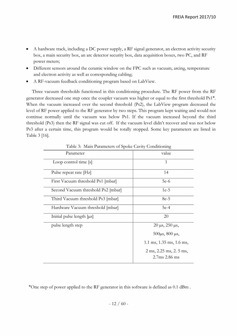
Table 3: Main Parameters of Spoke Cavity Conditioning

Parameter value

Loop control time [s] 1

Pulse repeat rate [Hz] 14

First Vacuum threshold Ps1 [mbar] 5e-6

Second Vacuum threshold Ps2 [mbar] 1e-5

Third Vacuum threshold Ps3 [mbar] 8e-5

Hardware Vacuum threshold [mbar] 5e-4

Initial pulse length [µs] 20

pulse length step 20 µs, 250 µs,

500µs, 800 µs,

1.1 ms, 1.35 ms, 1.6 ms,

2 ms, 2.25 ms, 2. 5 ms,

2.7ms 2.86 ms

*One step of power applied to the RF generator in this software is defined as 0.1 dBm .


- 13 / 60 -

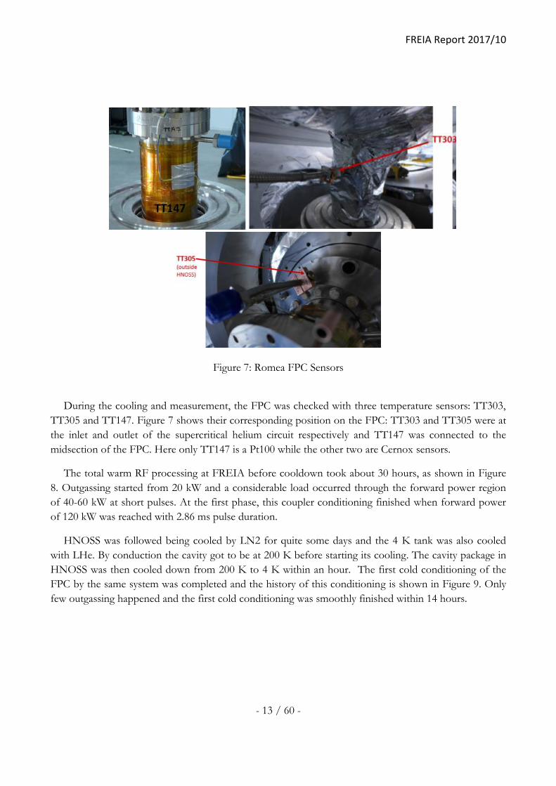
Figure 7: Romea FPC Sensors

During the cooling and measurement, the FPC was checked with three temperature sensors: TT303,

TT305 and TT147. Figure 7 shows their corresponding position on the FPC: TT303 and TT305 were at

the inlet and outlet of the supercritical helium circuit respectively and TT147 was connected to the

midsection of the FPC. Here only TT147 is a Pt100 while the other two are Cernox sensors.

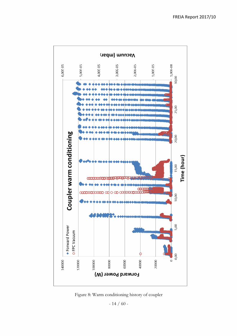
The total warm RF processing at FREIA before cooldown took about 30 hours, as shown in Figure

8. Outgassing started from 20 kW and a considerable load occurred through the forward power region

of 40-60 kW at short pulses. At the first phase, this coupler conditioning finished when forward power

of 120 kW was reached with 2.86 ms pulse duration.

HNOSS was followed being cooled by LN2 for quite some days and the 4 K tank was also cooled

with LHe. By conduction the cavity got to be at 200 K before starting its cooling. The cavity package in

HNOSS was then cooled down from 200 K to 4 K within an hour. The first cold conditioning of the

FPC by the same system was completed and the history of this conditioning is shown in Figure 9. Only

few outgassing happened and the first cold conditioning was smoothly finished within 14 hours.


- 14 / 60 -

Figure 8: Warm conditioning history of coupler


- 15 / 60 -

Figure 9: First cold conditioning of coupler


- 16 / 60 -

Second cold conditioning 4.2.

In order to reach high efficiency and high availability by reducing the time and effort of the overall

conditioning process, an automatic conditioning system, which consists of an acquisition system, a

control system based on LabView software and feedback was developed at FREIA [17]. Figure 10 shows

a typical interface of FREIA’s automatic RF conditioning control program. The drive power level to the

RF station could be controlled either manually or by this automatic conditioning system, while all

essential safety interlocks were implemented in hardware. Some sensors and interlock signal came from

IPN Orsay’s system in this test, while the conditioning program and other hardware used were FREIA’s

own.

Figure 10: The control screen of the FREIA automatic RF conditioning system.

RF power conditioning with the FREIA system was done in standing wave with the same pulse

lengths regime from 20 to 2860 μs. During each phase of selected pulse length, the power started from a

low value and then ramped up step by step depending on various operating parameters. Finally, the

maximum power of 120 kW was reached. Two software vacuum thresholds were adopted in this

conditioning procedure: as long as the coupler vacuum kept below the first software threshold of 5e-7

mbar, RF power increased, and once above the first software threshold, the controller held the RF

output until the vacuum was recovered. Otherwise, RF power was decreased by 1dB if the vacuum got

worse than the second threshold of 1e-6 mbar. Note that this 1 dB power drop only applied once in


- 17 / 60 -

each outgassing above the second threshold. Based on the conditioning experience from worldwide

laboratories, the coupler vacuum usually recovers in most of the cases while a few harsh outgassing

becomes worse fast and triggers the hardware interlock. Once the current phase reached the targeted

power, the system kept the maximum forward power for a soaking time before the input signal was cut

off. The next phase should not be executed until the vacuum recovered below the first threshold. In

parallel, an interlock system protected the RF components independently. Essential detective activities

employed in the interlocks were arc, electronic events, temperature and vacuum. The main software

control parameters are shown in Table 4.

Table 4: Main Parameters of Spoke Cavity Conditioning

Parameter value

Loop control time [s] 1

Pulse repeat rate [Hz] 14

Vacuum upper limit [mbar] 1e-6

Vacuum lower limit [mbar] 5e-7

Initial pulse length [µs] 20

pulse length step

20 µs, 50 µs,

100 µs, 200 µs,

500 µs, 1ms, 1.5 ms, 2 ms,

2.5 ms, 2.86 ms

The main devices for the RF conditioning process are:

Signal Generator

Power Meter

Vacuum Gauge

Arc Detector

Electron Detector

Fast RF Interlock Switch

Vacuum Pumping System

The FREIA automatic RF conditioning control program is based on LabView platform, with

functions reading or publishing data from/to EPICS system. The whole program consists of several

modules to make debugging easier and future upgrading more flexible. This conditioning system was

then tested with the ESS cavity package to verify the logic and related hardware. The overall FREIA

system worked as expected: with little vacuum activity the forward power quickly ramped up to 120 kW


- 18 / 60 -

with 2.86 ms. The well performance of FREIA’s automatic conditioning system implies that it is ready

for future conditioning missions.

5. Cavity package conditioning A major difference, compared to the FPC conditioning, is that the cavity RF conditioning was done by

the pulsed self-excited loop as describe in chapter 3.

The cavity conditioning had been implemented above operational power level in two phases. The

first phase introduced a frequency modulation (FM) around the resonant frequency at a very low power

level in order to sweep the field distribution forth and back along the coupler walls in a controlled

manner. The FM modulation was completed by a digital phase shifter based on NI FlexRIO FPGA and

NI 5782R data acquisition modules. With this digital system, the loop delay could be varied with high-

precision, where the loop delay is tightly related to loop frequency. The subsequent phase was also

completed with the SEL but only by ramping up the RF power with a fixed pulse length of 2.86 ms,

which gave a higher efficiency for conditioning.

Figure 11 shows the cavity package conditioning history. Three major multipacting (MP) regions have

been found during the cavity package conditioning, with key parameters shown in Table 5. The first MP

happened during the forward power from 22 to 30 kW, corresponding to a flattop accelerating gradient

from 4.5 to 4.8 MV/m. This MP was accompanied with a degrading coupler vacuum and higher electron

current, which most likely happened at the area close to the interface between the cavity and coupler.

The second MP barrier encountered was from 35 to 48kW with a flattop gradient from 5.2 to 5.7 MV/m.

While going through the third region from 67 to 76 kW, which was roughly from 7 to 7.5 MV/m, the

performance of the cavity was stable. High X-ray activity was detected during the heavy MP, which

caused an increase of the coupler temperature. Radiation was swapping between very high and low levels.

After about 30 hours of conditioning, the cavity package reached and was stably kept at 9MV/m flattop

accelerating gradient for more than 3 hours. The corresponding forward power was 110 kW. During

further measurements, all these three MP regions were repeatable but much easier to go through and

with less radiation.

Table 5: Major MP region during Spoke Cavity Conditioning

MP barrier Flattop gradient [MV/m] RF input power [kW]

1 4.5 - 4.8 22 - 30

2 5.2 - 5.7 35 - 48

3 7 - 7.5 67 - 76


- 19 / 60 -

Figure 11: Cavity package conditioning history


- 20 / 60 -

6. Quality factor measurement and dynamic heat load

Cool down procedure 6.1.

The time it takes to cool down HNOSS' shield from room temperature depends on the chosen final

value. Initially, the cooldown went fast (especially for the ICB) but below 120 K the cooling rate was

much lower. If one considers the shield to be cold when all sensors placed around the LN2 shield (both

in the VB and the cryostat) is less than 120 K, then the time it took to cool down from room

temperature to 120 K was 21.5 hrs. Afterwards, the cavity package in HNOSS was cooled down from

200K to 4K within an hour. Figure 12 shows the cooldown history, from which an average cooling rate,

bigger than 1 K/min was kept in the temperature region from 150 to 75 K, to avoid Q-disease in the

cavity.

The cooldown rates for this run for Romea were considered from the start temperature of 205 K.

Different cooldown rates based on different calculation conditions are:

4.1 K/min : if all TTs (except TT125) ≤ 20 K

3.25 K/min : if 150 K ≤ all TTs (except TT125) ≤ 20 K

4.48 K/min: if 150 K ≤ all TTs (except TT125 and TT104) ≤ 20 K

Note that the starting temperature of Romea (ca. 200K) for cooldown was achieved by first cooling

the cryostat shield with LN2 for four days after the conditioning of the FPC at room temperature (end

temperature 250 K) and the last 50 K decrease came when the sequence for cooling the 4K tank was

started. More details about the cooldown can be seen in [18].

Figure 12: Cooldown history of Romea cavity package


- 21 / 60 -

During cooldown, the resonant frequency of Romea was checked via an S parameter measurement to

study the cavity behavior. These measurements will help with the frequency control during the cavity

fabrication and post-processing. The cavity resonant frequency shifts as a function of temperature are

shown in Figure 13 and Figure 14. Table 6 lists the key frequencies of Romea at three different

temperatures, from which the frequency increment due to cryo-constriction was about 500 kHz from

300 K to 4 K, while a frequency decreasing of 27 kHz happened from 4 K to 2 K since the helium

pressure decrease from 1 atmosphere to 30 mbar.

Table 6: Resonant frequency of Romea

Temperature Resonance frequency Frequency shift [MHz] Frequency shift [%]

300 K 351.8939± 0.0005MHz -- --

4 K 352.4004 ± 0.0005MHz -0.507 ± 0.001 0.144

2 K 352.3725 ± 0.0005MHz -0.479 ± 0.001 0.136

Figure 13: Cavity frequency checking during cooldown from 200 K to 4 K. Here, the red curve is

temperature of the cavity, blue curve is the cavity frequency and the black curve the pressure in the

helium tank.


- 22 / 60 -

Figure 14: Cavity frequency checking during cooldown from 4 K to 2 K. Here, the red curve is

temperature of the cavity, blue curve is the cavity frequency and the black curve the pressure in the

helium tank.

Quality factor measurement 6.2.

The quality factor measurement of the cavity package was based on the calorimetrical method. The

cavity package was operated at a pulse mode with 14 Hz repetition rate and 2.86 ms duration. Limited by

the FPC, peak power was 120 kW, which still adequately built a field with a flattop gradient of 9 MV/m.

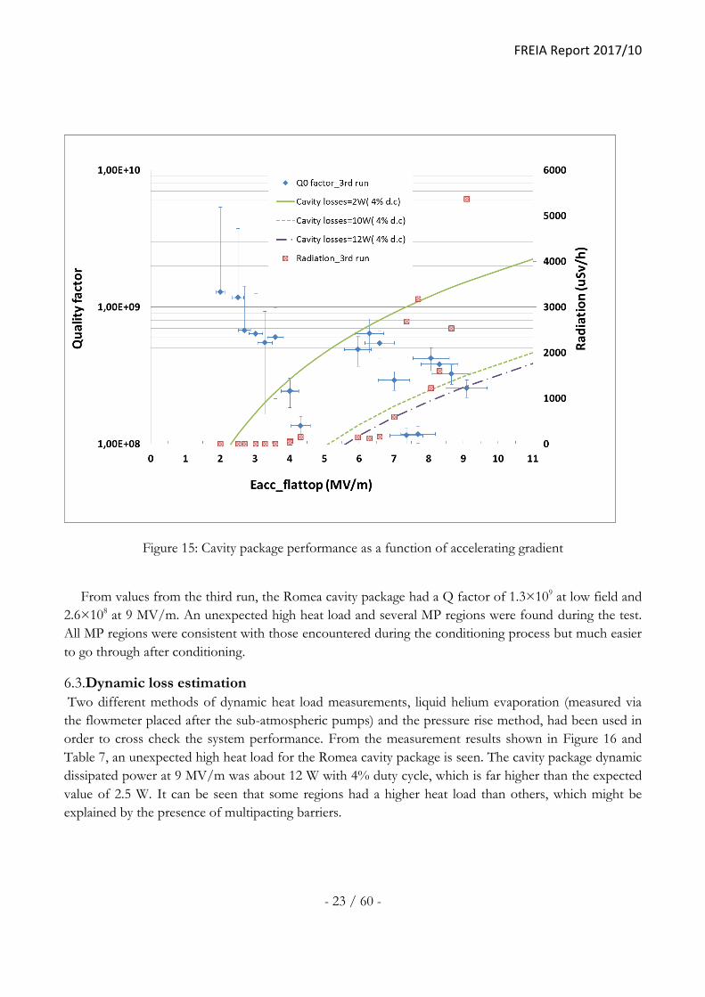
The preliminary result of the quality factor of the cavity package vs. gradient curve is shown in Figure 15.

The high power test of the spoke cavity package started in April 2017 and lasted until shipping it back to

IPN Orsay in May 2017.

In general, the measurements could be divided into three runs. The major difference among the test

runs is the use of different test methods and condition controls for the heat load measurement. In the

first run, the heat load was only measured by the helium gas flowmeter at room temperature and

pressure. The second and third runs used both the pressure rise method and the flowmeter method but

under different conditions. During the second run, the heat load was determined once parameters such

as helium flow, coupler temperature and helium pressure were stable. During the third run the system

was left to stabilize only in cavity pressure (See section 6.3 for more information).


- 23 / 60 -

Figure 15: Cavity package performance as a function of accelerating gradient

From values from the third run, the Romea cavity package had a Q factor of 1.3×109 at low field and

2.6×108 at 9 MV/m. An unexpected high heat load and several MP regions were found during the test.

All MP regions were consistent with those encountered during the conditioning process but much easier

to go through after conditioning.

Dynamic loss estimation 6.3.

Two different methods of dynamic heat load measurements, liquid helium evaporation (measured via

the flowmeter placed after the sub-atmospheric pumps) and the pressure rise method, had been used in

order to cross check the system performance. From the measurement results shown in Figure 16 and

Table 7, an unexpected high heat load for the Romea cavity package is seen. The cavity package dynamic

dissipated power at 9 MV/m was about 12 W with 4% duty cycle, which is far higher than the expected

value of 2.5 W. It can be seen that some regions had a higher heat load than others, which might be

explained by the presence of multipacting barriers.


- 24 / 60 -

Figure 16: Dynamic loss vs. accelerating gradient


- 25 / 60 -

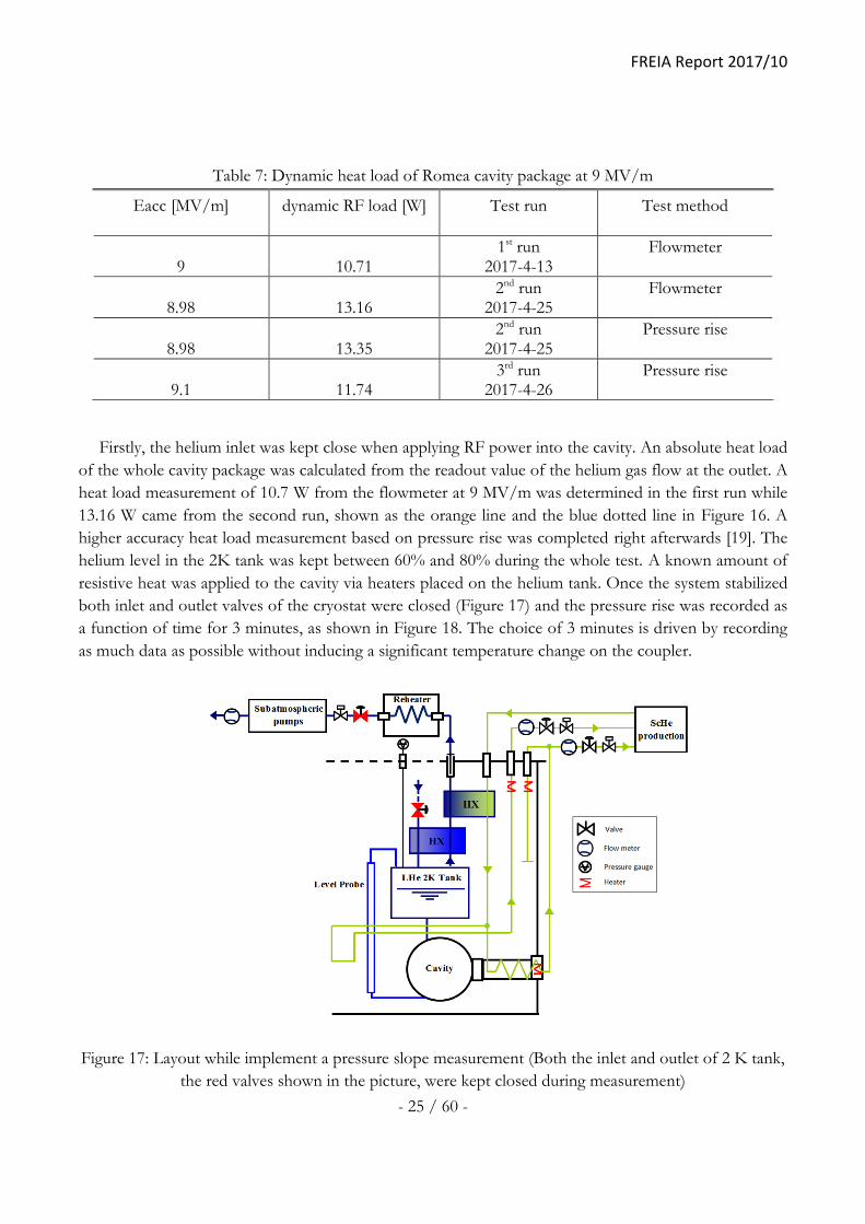
Table 7: Dynamic heat load of Romea cavity package at 9 MV/m

Eacc [MV/m] dynamic RF load [W] Test run Test method

9 10.71 1st run

2017-4-13 Flowmeter

8.98 13.16 2nd run

2017-4-25 Flowmeter

8.98 13.35 2nd run

2017-4-25 Pressure rise

9.1 11.74 3rd run

2017-4-26 Pressure rise

Firstly, the helium inlet was kept close when applying RF power into the cavity. An absolute heat load

of the whole cavity package was calculated from the readout value of the helium gas flow at the outlet. A

heat load measurement of 10.7 W from the flowmeter at 9 MV/m was determined in the first run while

13.16 W came from the second run, shown as the orange line and the blue dotted line in Figure 16. A

higher accuracy heat load measurement based on pressure rise was completed right afterwards [19]. The

helium level in the 2K tank was kept between 60% and 80% during the whole test. A known amount of

resistive heat was applied to the cavity via heaters placed on the helium tank. Once the system stabilized

both inlet and outlet valves of the cryostat were closed (Figure 17) and the pressure rise was recorded as

a function of time for 3 minutes, as shown in Figure 18. The choice of 3 minutes is driven by recording

as much data as possible without inducing a significant temperature change on the coupler.

Figure 17: Layout while implement a pressure slope measurement (Both the inlet and outlet of 2 K tank,

the red valves shown in the picture, were kept closed during measurement)


- 26 / 60 -

Figure 18: Different pressure rise as a function of time by a known resistance for 3 minutes (the step-

wise graph recorded from the EPIC system, the reason for where the steps came from is still under

study)

A heat load calibration curve was built by repetition of the relative pressure rise measurements. The

pressure gradient as a function of heat power fulfills the equation

𝑆𝑙𝑜𝑝𝑒𝑅𝐹 = 𝑆𝑙𝑜𝑝𝑒1𝑊 × 𝑃𝑑𝑦𝑛𝑎𝑚𝑖𝑐 + 𝑆𝑙𝑜𝑝𝑒𝑠𝑡𝑎𝑡𝑖𝑐 (6.1)

Where SlopeRF is the measured pressure gradient for a certain heat load,

Pdynamic is the corresponding dynamic heat load with respect to a certain SlopeRF, in [W],

Slope1W is the dynamic heat load coefficient in [1/W] ,

Slopestatic is a pressure gradient offset depends on the static heat load.

Through the calibration curve shown in Figure 19, the dynamic heat load calculation of Romea is,

𝑆𝑙𝑜𝑝𝑒𝑅𝐹 = 0.00155 × 𝑃𝑑𝑦𝑛𝑎𝑚𝑖𝑐 + 0.015 (6.2)

Finally, RF power was loaded in the cavity and the dynamic load was calculated by using this

calibration curve. The dynamic heat load of Romea’s cavity package as a function of the accelerating

gradient during the second run is shown as a solid blue line in Figure 16. A dynamic heat load of 13.35

W was found at 8.98 MV/m.


- 27 / 60 -

Figure 19: Calibration pressure gradient as a function of heat power

The heat load measurement based on the pressure rise method had been implemented in the second

and third runs. Each measured point was determined once all parameters got stable in the second run,

and the waiting time for each point, mainly due to a slow recovery of the coupler temperature, was

roughly 30 mins. Here, the coupler temperature was considered to be good enough when TT147 was

below 40 K. In this way, to obtain a whole measured curve of the dynamic heat load as a function of

gradient needs almost a working day. Two different methods, both flowmeter method and pressure rise

method were used to crosscheck the result and showed a good agreement with each other in the second

run. Considering the cryo-parameters were relatively slow changing compared to the helium tank

pressure, the system was left to stabilize only in pressure and recorded the pressure rise in the third run.

The test efficiency was thus improved by a shorter measurement time with more measurement points.

All measurement points of dynamic heat load during the third run are listed in Table 8.


- 28 / 60 -

Table 8: Dynamic heat load of Romea cavity package in the third run

Eacc [MV/m] pressure rise slop dynamic RF load [W]

2.00 0.0152 0.13

2.52 0.0153 0.19

2.70 0.0156 0.39

3.03 0.0158 0.52

3.29 0.0161 0.71

3.59 0.0162 0.77

4.01 0.0187 2.39

4.32 0.0227 4.97

5.32 0.0359 13.48

5.97 0.0191 2.64

6.30 0.0185 2.26

6.59 0.0195 2.90

7.01 0.0245 6.13

7.36 0.0413 16.97

7.70 0.0432 18.19

8.07 0.0237 5.61

8.31 0.0252 6.580

8.66 0.028 8.39

9.10 0.0332 11.74


- 29 / 60 -

Hypothesis for the high heat loads measured 6.4.

When the cavity was operating at its design field, a high radiation of 6 mSv/h at 90 degree angle of

beam direction was observed. High radiation implies that MP or field emission happened in the cavity

package, and it leads to high heat load and low Q factor. Possible causes have been considered and

corresponding improvements are being studied. Considerations are focusing on the following five

hypotheses: a contaminated FPC, debris generated during conditioning cryopumped on the cavity’s

surface, FPC is not fully conditioned, a bigger impact on heat load than expected from the FPC into the

cavity or a combination of all these.

Firstly, the FPC might have been polluted either during assembly or during its conditioning. There

were two FPC installed back-to-back during the conditioning at IPN Orsay. The ceramic window of the

neighbouring FPC was broken and a pressure of a few mbar was reached. Particles from the ceramic

window and air may have reached Romea's FPC, and since there was no processing of Romea's FPC

after this incident they might have remained, although before the assembly of the coupler, the particles

on the coupler smaller than 0.3 µm were counted by blowing filtered nitrogen and no problems were

found. This could still mean that the coupler could have been polluted not in surface but deeper, which

might be probably true for the double-wall tube, where the particles may have been trapped into the

coated layer of copper. After returning the cavity back to IPN Orsay, the FPC was detached and they

could see that the ceramic window was completely sputtered with copper. This must have happened

during the conditioning or RF tests at FREIA since before assembly IPN Orsay saw that the ceramic

window was white before assembly. The situation of ceramic reinforces the theory that the FPC might

have been contaminated.

Secondly, during the cold conditioning of the coupler and the cavity package, the cavity was cold and

worked as a cryo pump. The particles released during the conditioning could have contaminated the

cavity’s surface. This hypothesis is reinforced by the poor vacuum (10-3 mbar) reached in the cavity

during warm up (Figure 20). At the beginning of the warm up, both FPC and cavity had a significant

outgassing at around 5-10 K, which implies that hydrogen could be the major trapped gas. A second

outgassing point of the coupler started from around 40 K with a vacuum in the order of 10-4 mbar. In

this step, oxygen became the dominating vapor element. During warm up, only an ion pump was used at

the beginning and it stopped running due to the high vacuum levels reached. A turbo pump was then

started so the vacuum system recovered quickly and afterwards the ion pump could be restarted. Both

the cavity’s and the FPC’s vacuum got better and was below 10-5 mbar in a short time.


- 30 / 60 -

Figure 20: Vacuum curve at warm up


- 31 / 60 -

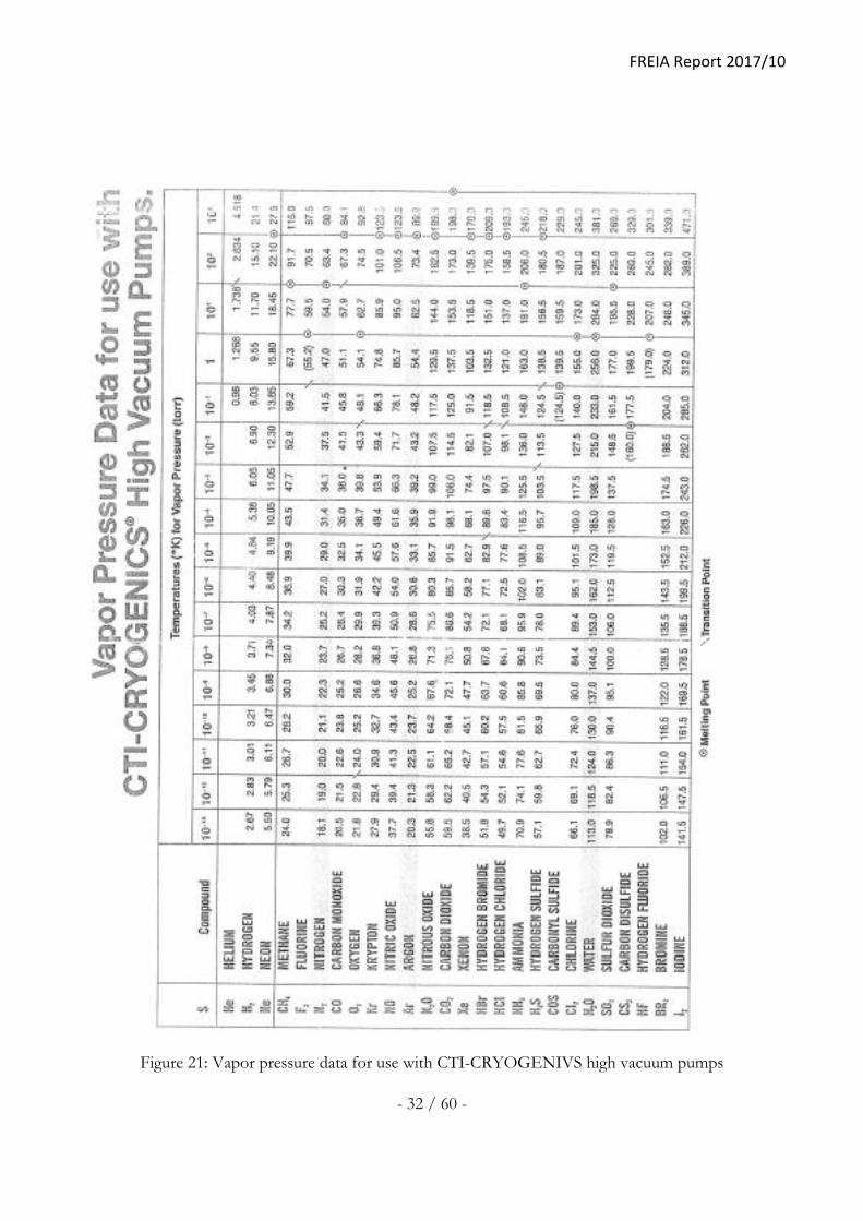
With respect to the vapor pressure data table shown in Figure 21[20], hydrogen is fully vaporized and

released above 20 K. The easiest and most efficient solution for avoiding hydrogen trapping is warming

up the whole package up to 30-40 K with both turbo pump and ion pump for a certain time, 30 minutes

as an example in PLS facility and around 40-60 minutes in SOLEIL accelerator [21]. To fully release the

oxygen a temperature above 90 K is needed, at which point a cavity also has a risk of getting Q-disease.

In Romea’s case, a new post processing of 650 °C baking has been done. No more risk of Q-disease

effect was verified at the vertical test at IPN Orsay. Therefore, a warm up after cavity package

conditioning up to 40 K or 90 K would be highly recommended for the ESS double spoke cavity to

improve the cavity performance as well as to reduce the system’s dynamic heat load. With the help of a

mass spectrometer, the outgassing components could be thoroughly studied. Also, installing one extra

pump at the coupler side would significantly improve the pumping efficiency and would be very helpful

in avoiding contamination in the cavity wall. To this end, one ‘T’ type pipe could be added at the

position of the current vacuum sensor near the ceramic window, which would allow one to connect an

extra pumping system. In the case of Romea though (and all double spoke cavities for ESS), the

pumping efficiency might not be so high since the available port is 6 mm in diameter and the space

around the window is already quite tight. Placing this tee would mean moving the vacuum gauge further

away from the ceramic. Note also that the installation of piping needs an exposure of the coupler

vacuum to air, which should be completed in a clean room.

Another hypothesis is that due to the tight time schedule, with a 4% duty pulse conditioning, the FPC

might be still not fully conditioned. The residual contamination on the FPC can lead to the stubborn MP

barriers that have been seen in the test. To reduce the impact of MP in the coupler, adding a high

voltage bias would be highly recommended. This DC bias is currently being added by IPN Orsay to the

design of the FPC.

Last but not least, the coupler temperature was higher than expected with RF on. The temperature

sensor, TT147 attached between helium gas inlet and outlet, was around 40 K when no MP happened

and increased rapidly up to 105K during MP. The heat from the coupler transferred to the cavity could

cause a higher heat load if cooling of the FPC's has a great impact on the total heat load. According to

the further study result from cryogenic measurement, the coupler at 90 K in the midsection (TT147)

would only increase 1 W heat load [22]. Therefore, this point is not likely to be the dominating cause for

the high heat load. Note that no solid study of temperature at the interface of coupler and cavity wall has

been done since no temperature sensor was installed there. In next runs, more temperature sensors will

be attached to the locations of interest for monitoring the cavity wall temperature.


- 32 / 60 -

Figure 21: Vapor pressure data for use with CTI-CRYOGENIVS high vacuum pumps


- 33 / 60 -

Error estimation 6.5.

6.5.1. Gradient measurement uncertainty

Equation (6.3) gives the definition of accelerating gradient. In practice, the flattop gradient can be

obtained either through the transmitted or the forward power. In this test run, the results from two

independent methods were used to cross-check the flattop accelerating gradient, with the related formula

given in Equation (6.4) and (6.5).

𝐸𝑎𝑐𝑐 =𝑉𝑐

𝐿𝑒𝑓𝑓 (6.3)

𝐸𝑎𝑐𝑐_𝑝𝑒𝑎𝑘_𝑃𝑡 =√𝑅

𝑄⁄ × 𝑃𝑡_𝑚𝑎𝑥 × 𝑄𝑡

𝐿𝑒𝑓𝑓 (6.4)

𝐸𝑎𝑐𝑐_𝑝𝑒𝑎𝑘_𝑃𝑓 = √4 × 𝑅𝑄⁄ × 𝑄𝐿 × 𝑃𝑓_𝑚𝑎𝑥 (6.5)

Where 𝑉𝑐 is the cavity voltage, in [V],

𝐿𝑒𝑓𝑓 is the effective accelerating length, in [m],

𝑃𝑡_𝑚𝑎𝑥 is the maximum transmitted power at the flattop gradient, in [W],

𝑄𝑡 is the external quality factor of the pick-up antenna,

𝑅 𝑄⁄ is the shunt impedance of the cavity, in [Ω],

𝐸𝑎𝑐𝑐_𝑝𝑒𝑎𝑘_𝑃𝑡 is the flattop gradient calculated via Pt_max, in [MV/m],

𝑄𝐿 is the loaded quality factor of the cavity,

𝑃𝑓_𝑚𝑎𝑥 is the maximum forward power during the pulse, in [W],

𝐸𝑎𝑐𝑐_𝑝𝑒𝑎𝑘_𝑃𝑓 is the the flattop gradient calculated via Pf_max, in [MV/m].

Most of the error propagation of an equation of the type x= f(u,v) can be done by using the

following fundamental equation[23]

𝜎𝑥2 = 𝜎𝑢

2(𝜕𝑥

𝜕𝑢)2 + 𝜎𝑣

2(𝜕𝑥

𝜕𝑣)2 + 2𝜎𝑢𝑣

2 (𝜕𝑥

𝜕𝑢) (

𝜕𝑥

𝜕𝑣) (6.6)

If u and v are uncorrelated, then 𝜎𝑢𝑣2 = 0.

In the case of 𝐸𝑎𝑐𝑐_𝑝𝑒𝑎𝑘_𝑃𝑡 measurement, 𝑄𝐿 and 𝑃𝑡_𝑚𝑎𝑥 come from independent measurement. The

propagation of errors of the flattop gradient thus can be simplified as


- 34 / 60 -

∆ 𝐸𝑎𝑐𝑐_𝑝𝑒𝑎𝑘_𝑃𝑡

𝐸𝑎𝑐𝑐_𝑝𝑒𝑎𝑘_𝑃𝑡=

1

2√(

∆𝑄𝑡

𝑄𝑡)2 + (

∆𝑃𝑡

𝑃𝑡)2 (6.7)

Uncertainty of 𝑄𝑡 measurement

𝑄𝑡 value came from the latest vertical test at IPN Orsay. Since there was no adjustment of the

pick-up antenna before the high power test, ∆𝑄𝑡

𝑄𝑡 is assumed to be not worse than 10%.

Uncertainty of transmitted power measurement

The uncertainty of the transmitted power measurement usually is given by

∆𝑃𝑡

𝑃𝑡= √(𝛿𝐶𝑡)2 + (

∆𝑃𝑡𝑚

𝑃𝑡𝑚)2 (6.8)

𝑃𝑡 = 𝑃𝑡𝑚 × 𝐶𝑡 (6.9)

∆𝑃𝑡𝑚 = 𝑃𝑡𝑚 × 𝛿𝑃𝑐𝑎𝑙 + 𝑃𝑚𝑖𝑛 (6.10)

Where 𝑃𝑚𝑖𝑛 is the sensitivity limit of the power sensor, in [W],

𝛿𝑃𝑐𝑎𝑙 is the fractional uncertainty in the absolute power measurement,

𝛿𝐶𝑡 is the fractional uncertainty in cable calibration,

∆𝑃𝑡𝑚 is the error in 𝑃𝑡 , in [W].

Keysight N1912A power meters were adopted for all power measurements in this test run,

which aim for accurate power reading with low measurement noise. 2 µW of sensitivity limit for

the power sensor was negligible in the error calculation. Therefore the measurement uncertainty

of the transmitted power is recalculated as

∆𝑃𝑡

𝑃𝑡= √(𝛿𝐶𝑡)2 + (𝛿𝑃𝑐𝑎𝑙)2 (6.11)

Uncertainty of an absolute power measurement

The fractional uncertainty in an absolute power measurement depends on the significant

uncertainties throughout the measurement. Table 9 summarizes the statistical characteristics of

each source of uncertainty [24]. All items, except mismatch uncertainty, come from the

specifications of E9322A sensor and Keysight N1912A power meter over a temperature range

of 25 ± 10 °C. Mismatch uncertainty is however dependent on the local loop setting, which is


- 35 / 60 -

calculated from the specified standing wave ration (SWR) of the device and the sensor, as shown

in Equation (6.12). In the pulsed SEL (shown in Figure 4), both the 4-way splitter and the power

sensor contributed to the mismatch uncertainty. The SWR of the 4-way splitter and the power

@350 MHz sensor were about 1.2.

𝑈𝑚𝑖𝑠𝑚𝑎𝑡𝑐ℎ = ±𝑆𝑊𝑅𝑠𝑝𝑙𝑖𝑡𝑡𝑒𝑟 − 1

𝑆𝑊𝑅𝑠𝑝𝑙𝑖𝑡𝑡𝑒𝑟 + 1×

𝑆𝑊𝑅𝑠𝑒𝑛𝑠𝑜𝑟 − 1

𝑆𝑊𝑅𝑠𝑒𝑛𝑠𝑜𝑟 + 1× 100% (6.12)

Table 9: Significant uncertainty in an absolute power measurement

Identify significant uncertainty Value

Meter uncertainty ±0.8%

Zero uncertainty ±0.015%

Sensor calibration uncertainty ±4.2%

Standard uncertainty of mismatch ±0.8%

Two methods are commonly used to combine power measurement uncertainties: worst-case

and Root Sum of the Squares (RSS) [24]. The RSS method is considered as a more realistic

approach to combine uncertainties and can be calculated by Equation (6.13). It is based on the

fact that most of the errors, although systematic, are independent and therefore could be

combined as random variables. This allows to apply the RSS method in the statistical

combination. In this way, only the RSS uncertainty was considered in our case.

𝑈𝑐 = √(𝑈𝑚𝑖𝑠𝑚𝑎𝑡𝑐ℎ

√2)2 + (

𝑠𝑦𝑠𝑟𝑠𝑠

2)

2

(6.13)

Where 𝑠𝑦𝑠𝑟𝑠𝑠 is the RSS of the meter uncertainty, the zero uncertainty and the sensor

calibration uncertainty.

With the significant uncertainty values of the power measurement at FREIA, the combined

standard uncertainty was ± 2.2% and the expanded uncertainty was ± 4.4% [24]. Note that only

the expanded uncertainty was used as the uncertainty of an absolute power measurement from a

power meter in all following calculations.

Uncertainty of cable calibration

The cable calibration for the transmitted power included two parts: S11 measurement of the

cryo-cable (from the pick-up antenna to the feedthrough in the cryostat) and the absolute power

measurement of the cable from cryostat to the control room at warm. For the warm path

calibration, a signal generator was first calibrated against a power meter for an absolute power

measurement and later used as a power source and reference. Another absolute power


- 36 / 60 -

measurement was completed by the on-site power meter. The difference between these two

power readings was the losses on the path. The fractional uncertainty in cable calibration was

calculated as

𝛿𝐶𝑡 = √(∆𝑆11

𝑆11)2 + (

∆𝑃1

𝑃1)2 + (

∆𝑃2

𝑃2)2 (6.14)

With the uncertainty of ±2.3% of the S11 measurement using a VNA (N5221) and the

expanded uncertainty ± 4.4% of the absolute power measurement, the fractional uncertainty in

cable calibration of 6.6% was obtained.

Uncertainty of accelerating gradient

Considering that the sensor calibration uncertainty did not drift significantly within the power

range, one substituted Equations (6.11) in Equation (6.7) and obtained the accelerating gradient

uncertainty of 6.4%.

6.5.2. Heat load measurement uncertainty

Two different methods had been applied to the heat load measurement. The measurement accuracy of

liquid helium evaporation method mainly relied on the flowmeter measurement placed after the sub-

atmospheric pumps. It had a better accuracy at higher heat load, more details and error estimation can

be found in [18]. This section will only discuss the measurement uncertainty of the pressure rise method

calculated by

𝑆𝑙𝑜𝑝𝑒𝑅𝐹 = 𝑆𝑙𝑜𝑝𝑒1𝑊 × 𝑃𝑑𝑦𝑛𝑎𝑚𝑖𝑐 + 𝑆𝑙𝑜𝑝𝑒𝑠𝑡𝑎𝑡𝑖𝑐 (6.1)

Uncertainty of pressure gradient measurement

The linear regression was applied to every pressure gradient measurement. With a given set of

time measurement x and corresponding instantaneous helium pressure y, the pressure gradient is

given by a least-square fitting [25]

𝑦 = 𝑎𝑥 + 𝑏

The uncertainty 𝜎𝑖 associated with each pressure measurement 𝑦𝑖 was known, and that of the

time measurement done by a data acquisition system was so small therefore that it was neglected.

The best-fit model parameters 𝑎, 𝑏 and corresponding uncertainties are calculated as


- 37 / 60 -

𝑎 =𝑆𝑥𝑥𝑆𝑦 − 𝑆𝑥𝑆𝑥𝑦

∆

𝑏 =𝑆𝑆𝑥𝑦 − 𝑆𝑥𝑆𝑦

∆

𝜎𝑎2 =

𝑆𝑥𝑥

∆

𝜎𝑏2 =

𝑆

∆ (6.15)

Namely, 𝑎 is the pressure gradient 𝑆𝑙𝑜𝑝𝑒𝑅𝐹 at a certain applied power and 𝜎𝑎 is its

uncertainty.

Where according to the fundamental error estimation of a least-square fitting, following sums

are defines as

𝑆 ≡ ∑1

𝜎𝑖2

𝑁

𝑖=1

𝑆𝑥 ≡ ∑𝑥𝑖

𝜎𝑖2

𝑁

𝑖=1

𝑆𝑦 ≡ ∑𝑦𝑖

𝜎𝑖2

𝑁

𝑖=1

𝑆𝑥𝑥 ≡ ∑𝑥𝑖

2

𝜎𝑖2

𝑁

𝑖=1

𝑆 ≡ ∑𝑥𝑖𝑦𝑖

𝜎𝑖2

𝑁

𝑖=1

∆≡ 𝑆𝑆𝑥𝑥 − (𝑆𝑥)2 (6.16)

Uncertainty of 𝑆𝑙𝑜𝑝𝑒1𝑊 and 𝑆𝑙𝑜𝑝𝑒𝑠𝑡𝑎𝑡𝑖𝑐

The heat load calibration curve consisted of pressure gradients at different heater power. The

pressure gradient offset due to the static heat load (𝑆𝑙𝑜𝑝𝑒𝑠𝑡𝑎𝑡𝑖𝑐 ) and the pressure gradient

increment per dynamic heat load ( 𝑆𝑙𝑜𝑝𝑒1𝑊 ) were calculated by linear fitting of pressure

gradients and heater powers. The pressure at each certain power was measured for 3 minutes and

the corresponding pressure gradient was given by the linear regression. The uncertainty of each

linear regression calculated by Equation (6.15) was therefore re-used for the calculation of the

uncertainty of the calibration curve as given in Equation (6.2) and graphically in Figure 19.


- 38 / 60 -

Figure 22 : Pressure gradient calibration data at different heater power

Table 10: Uncertainty of each pressure measurement at different power level

Heater power [W]

Uncertainty of each pressure

measurement [mbar] Pressure gradient uncertainty

0 0.25 5.17×10-4

1 0.25 5.17×10-4

2 0.29 6×10-4

4 0.35 7.42×10-4

5 0.4 8.27×10-4

8 0.5 1.03×10-3

10 0.5 1.03×10-3

15 0.6 0.0012

Because of a conversion bug in the pressure data acquisition system, the pressure reading in

the system did not refresh at each sampling time. The pressure as function of time was a

stepwise display instead of a smooth curve, where the steps, no doubt, became the main source

of error in the pressure reading. As shown in Figure 22, the step had a trend to become bigger


- 39 / 60 -

when the heater power increased. Table 10 illustrates the uncertainty of each pressure

measurement at different heater power.

With a known heater power range from 0 to 15 W, the calibration curve was established with

the following parameters

𝑆𝑙𝑜𝑝𝑒1𝑊 = 0.00155 ± 4 × 10−5

𝑆𝑙𝑜𝑝𝑒𝑠𝑡𝑎𝑡𝑖𝑐 = 0.0150 ± 2 × 10−4

Using static heat load as the reference point

If Equation (6.1) used in the pressure rise method is rewritten, the dynamic heat load is

usually given by

𝑃𝑑𝑦𝑛𝑎𝑚𝑖𝑐 =𝑆𝑙𝑜𝑝𝑒𝑅𝐹 − 𝑆𝑙𝑜𝑝𝑒𝑠𝑡𝑎𝑡𝑖𝑐

𝑆𝑙𝑜𝑝𝑒1𝑊 (6.17)

Here, 𝑆𝑙𝑜𝑝𝑒𝑅𝐹, 𝑆𝑙𝑜𝑝𝑒𝑠𝑡𝑎𝑡𝑖𝑐 and 𝑆𝑙𝑜𝑝𝑒𝑅𝐹 are obtained from independent measurements and

the fractional uncertainty in a dynamic heat load measurement is

∆𝑃𝑑𝑦𝑛𝑎𝑚𝑖𝑐

𝑃𝑑𝑦𝑛𝑎𝑚𝑖𝑐= √

∆𝑆𝑙𝑜𝑝𝑒𝑅𝐹2 + ∆𝑆𝑙𝑜𝑝𝑒𝑠𝑡𝑎𝑡𝑖𝑐

2

（𝑆𝑙𝑜𝑝𝑒𝑅𝐹 − 𝑆𝑙𝑜𝑝𝑒𝑠𝑡𝑎𝑡𝑖𝑐）2+ (

∆𝑆𝑙𝑜𝑝𝑒1𝑊

𝑆𝑙𝑜𝑝𝑒1𝑊)2 (6.18)

The second part in the right hand side of Equation (6.18) represents the uncertainty of the

pressure gradient increment per dynamic heat load, which comes from the calibration and is a

constant over the whole measurement. The numerator of the first part consists of the square

sum of two pressure gradients, each in a range from 10-4 to 10-3 in this test run. Hence, it is

obvious that the denominator of the first part is the dominating part of the uncertainty of the

dynamic heat load.

When the cavity has a decent performance at low field, the RF loss is very small with respect

to the high quality factor, which means 𝑆𝑙𝑜𝑝𝑒𝑅𝐹 is close to 𝑆𝑙𝑜𝑝𝑒𝑆𝑡𝑎𝑡𝑖𝑐 and leads to

(𝑆𝑙𝑜𝑝𝑒𝑅𝐹 − 𝑆𝑙𝑜𝑝𝑒𝑠𝑡𝑎𝑡𝑖𝑐)2 ≅ 0

The fractional uncertainty of the dynamic heat load measurement at low field is thus huge. In

the case of Romea package test, as shown in Figure 23, the uncertainties for dynamic heat loads

less than 0.8 W, which corresponds to accelerating gradients lower than 4 MV/m, are higher

than 50%. On the other hand, the dynamic heat load is relatively higher when increasing the field,

so the denominator is further away from zero and the measurement uncertainty is reduced

significantly. In short, using the static heat load as a reference point has a better accuracy at


- 40 / 60 -

higher heat loads. An uncertainty of about 7% at 9 MV/m for the Romea package test was

obtained.

Figure 23: Uncertainty of the dynamic heat load by using static heat load as reference point. Note that

error bars in the graph are given in absolute value.

Using high heat load point as the reference point

The pressure gradient offset caused by the static heat load is dependent on an absolute

measurement. An alternative method using a reference point at high applied power was also

considered because, in general, a relative measurement and gives a higher accuracy than the

absolute one. The cavity package is a passive system and gives the same system characteristics for

different incident power, each two measurements of the pressure gradient fulfill

𝑆𝑙𝑜𝑝𝑒𝑟𝑒𝑓 = 𝑆𝑙𝑜𝑝𝑒1𝑊 ∗ 𝑃ℎ𝑒𝑎𝑡𝑒𝑟 + 𝑆𝑙𝑜𝑝𝑒𝑠𝑡𝑎𝑡𝑖𝑐

𝑆𝑙𝑜𝑝𝑒𝑅𝐹 = 𝑆𝑙𝑜𝑝𝑒1𝑊 ∗ 𝑃𝑑𝑦𝑛𝑎𝑚𝑖𝑐 + 𝑆𝑙𝑜𝑝𝑒𝑠𝑡𝑎𝑡𝑖𝑐 (6.19)

Where 𝑆𝑙𝑜𝑝𝑒𝑟𝑒𝑓 is the measured pressure gradient for a reference heat load,

𝑃ℎ𝑒𝑎𝑡𝑒𝑟 is the corresponding heat load with respect to 𝑆𝑙𝑜𝑝𝑒𝑟𝑒𝑓, in [W].

Solving Equation (6.19) for 𝑃𝑑𝑦𝑛𝑎𝑚𝑖𝑐 gives


- 41 / 60 -

𝑃𝑑𝑦𝑛𝑎𝑚𝑖𝑐 =𝑆𝑙𝑜𝑝𝑒𝑅𝐹 − 𝑆𝑙𝑜𝑝𝑒𝑟𝑒𝑓

𝑆𝑙𝑜𝑝𝑒1𝑊+ 𝑃ℎ𝑒𝑎𝑡𝑒𝑟 (6.20)

A relative high power reference point should be chosen for two reasons: (1) higher accuracy

for the heater power measurement and (2) higher accuracy for the pressure gradient fitting with

reference power. Heaters rated for a max applied power of 100 W were used in the test.

Therefore, a better linearity is obtained with a relative higher heater power. Also, with a constant

high applied power the helium pressure changes more significantly, which gives a better accuracy

in the pressure gradient measurement. In this run, a 15 W heater power was chosen as the

reference point.

The fractional uncertainty in a relative dynamic heat load measurement is

∆𝑃𝑑𝑦𝑛𝑎𝑚𝑖𝑐

𝑃𝑑𝑦𝑛𝑎𝑚𝑖𝑐= √

∆𝑆𝑙𝑜𝑝𝑒𝑅𝐹2 + ∆𝑆𝑙𝑜𝑝𝑒𝑟𝑒𝑓

2

（𝑆𝑙𝑜𝑝𝑒𝑅𝐹 − 𝑆𝑙𝑜𝑝𝑒𝑟𝑒𝑓）2+ (

∆𝑆𝑙𝑜𝑝𝑒1𝑊

𝑆𝑙𝑜𝑝𝑒1𝑊)2 + (

∆𝑃ℎ𝑒𝑎𝑡𝑒𝑟

𝑃ℎ𝑒𝑎𝑡𝑒𝑟)2 (6.21)

Compared to the absolute method, the denominator of the first part in the right hand side of

Equation (6.21) becomes the pressure gradient difference between the RF power and the

reference point. With a chosen high power reference point, the denominator can be well kept

away from zero. Therefore, lower heat losses in more accurate measurements can be obtained.

The third part represents the uncertainty of the heater power measurement at the reference

point. With the current set up, about 5% accuracy of the heater power measurement was

considered and used in the overall calculation.

In general, a superconducting cavity provides a good performance with very low dynamic

heat load. For example, one of the acceptance criteria of each ESS spoke cavities equipped with

FPC and CTS is < 2.5 W at 9 MV/m. In this way, this method provides accurate dynamic heat

load measurements in the whole gradient curve. Unfortunately, in Romea’s case some

contamination might have happened in the cavity leading to a high heat load in the MP regions

as well as at the high field. Heat loads around 15 W were close to the reference point of 15 W

heater power and therefore caused high uncertainty, as shown in Figure 24. From the result, the

heat load of 11.74 W at the nominal gradient gives an uncertainty of 45%.


- 42 / 60 -

Figure 24: Uncertainty of dynamic heat load by using 15 W power point as reference point. Note that

error bars in the graph are given in absolute value.

6.5.3. Unloaded Q measurement uncertainty

The unloaded quality factor Q0 of the cavity package running in a pulsed mode is calculated through

𝑄0 =𝑉𝑐_𝑎𝑣𝑒

2

𝑅𝑄⁄ × 𝑃𝑐𝑤

(6.22)

Where, 𝑉𝑐_𝑎𝑣𝑒 is the average cavity voltage built during the pulse and can be obtained via

Equation (6.27), 𝑃𝐶𝑊 is the continuous wave heat load with respect to the dynamic heat load

measured in the RF time, unit in [W], and can be obtained through Equation (6.24).

The uncertainty of an unloaded Q measurement at a certain gradient is given by

∆𝑄0

𝑄0= √(2

∆𝑉𝑐_𝑎𝑣𝑒

𝑉𝑐_𝑎𝑣𝑒)2 + (

∆𝑃𝑐𝑤

𝑃𝑐𝑤)2 (6.23)


- 43 / 60 -

Uncertainty of 𝑃𝐶𝑊

𝑃𝑐𝑤 = 𝑃𝑑𝑦𝑛𝑎𝑚𝑖𝑐 ×1

𝑇𝑅𝐹𝑅𝑟𝑒𝑝

⁄ (6.24)

Dividing the dynamic heat load by the duty factor of pulse can easily give the continuous wave

heat load at a certain gradient. Here, 𝑇𝑅𝐹 is the pulse duration (2.86 ms) and 𝑅𝑟𝑒𝑝 is repetition

rate (14 Hz).

Note that both the pulse duration and repetition rate were fixed during the measurement and

the minor error of the timing system in the LLRF was not considered in the calculation.

Therefore, the uncertainty of the continuous wave heat load was the same as the value of the

uncertainty of the dynamic heat load.

Uncertainty of cavity voltage measurement

During a pulsed mode measurement, the total RF power dissipated at the cavity wall

contributed to the heat load and was impossible to distinguish the fraction due only to the flattop

gradient. So the average cavity voltage is defined as the integration of the cavity voltage during

the pulse divided by the pulse duration.

At the FREIA high power test stand, the cavity voltage profile was recorded by the FPGA-

based program, in which the measured signal needed to be multiplied by a calibration factor to

convert to the true signal. A peak measurement of the transmitted power during a pulse was

continually done by the power meter. With the max transmitted power, the corresponding square

of max cavity voltage can be obtained by

𝑉𝑐_max _𝑃𝑡2 = R/Q × 𝑄𝑡 × 𝑃𝑡_𝑚𝑎𝑥 (6.25)

The integration of the cavity voltage profile then can be normalized

𝑉𝑐_𝑛𝑜𝑟𝑚2 =

∑ 𝑉𝑐_𝐹𝑃𝐺𝐴2 × ∆𝑡

𝑉𝑐_max _𝐹𝑃𝐺𝐴2 (6.26)

And used in

𝑉𝑐_𝑎𝑣𝑒2 =

𝑉𝑐_max _𝑃𝑡2×𝑉𝑐_𝑛𝑜𝑟𝑚

2

𝑇𝑅𝐹 (6.27)

Here, 𝑉𝑐_𝐹𝑃𝐺𝐴 is the cavity voltage at the certain stage during RF on,

𝑉𝑐_max _𝐹𝑃𝐺𝐴 is the maximum voltage during RF on,

∆𝑡 is the sampling time of 1 µs in the FPGA program.


- 44 / 60 -

Table 11: Maximum voltage measured by FPGA during the pulse in the third test run

Eacc [MV/m] 𝑉𝑐_max _𝐹𝑃𝐺𝐴[V]

2.00 0.149

2.52 0.187

2.70 0.201

3.03 0.223

3.29 0.242

3.59 0.265

4.01 0.295

4.32 0.318

5.32 0.393

5.97 0.439

6.30 0.464

6.59 0.484

7.01 0.515

7.36 0.541

7.70 0.566

8.07 0.594

8.31 0.611

8.66 0.636

9.10 0.669

The uncertainty of the cavity voltage measurement thus can be described as

∆𝑉𝑐_𝑎𝑣𝑒2

𝑉𝑐_𝑎𝑣𝑒2 = √(

∆𝑉𝑐_max _𝑃𝑡2

𝑉𝑐_max _𝑃𝑡2 )2 + (2

∆𝑉𝑐_max _𝐹𝑃𝐺𝐴

𝑉𝑐_max _𝐹𝑃𝐺𝐴)2 + (2

∑ ∆𝑉𝑐_𝐹𝑃𝐺𝐴

∑ 𝑉𝑐_𝐹𝑃𝐺𝐴)2 (6.28)


- 45 / 60 -

The first part of the right hand side in the Equation (6.28) represents the uncertainty of the

max transmitted power measurement, which is highly dependent on the absolute power

measurement. Equation (6.29) shows the uncertainty calculation in which the result of Equation

(6.11) is used as an input.

∆𝑉𝑐_max _𝑃𝑡2

𝑉𝑐_max _𝑃𝑡2 = √(

∆𝑄𝑡

𝑄𝑡)2 + (

∆𝑃𝑡_𝑚𝑎𝑥

𝑃𝑡_𝑚𝑎𝑥)2 (6.29)

The voltage error in the FPGA came from the ADC board capacity. The ADC board used at

FREIA provides 14 bits resolution and has no more than 50 µV variation in each voltage

sampling. Table 11 lists all the 𝑉𝑐_max _𝐹𝑃𝐺𝐴 during the third test run. Compared to the order of

uncertainty of the max transmitted power, this part has a very limited contribution.

Likewise, the uncertainty of the integration of the whole voltage profile was negligible in the

calculation.

Comparison of using different heat load method

Different heat load calculation methods affect the final uncertainty of the unloaded quality

factor measurement. This section will discuss the result from two different pressure rise method,

as shown in Figure 25 and Figure 15.

For the ESS goal of having as accurate measurement as possible around the operating

gradient, using the static heat load as a reference point in the pressure rise method provides a

smaller error bar at 9 MV/m. For this reason, it is motivated to use this method and the quality

factor with an error estimation shown in Figure 15 is chosen for the final display. Table 12 lists

the error estimation of Q0 measurement from 8 MV/m to 9 MV/m.


- 46 / 60 -

Figure 25: Uncertainty of quality factor measurement with using 15 W heater power as

reference point

Table 12: Error estimation of Q0 measurement from 8 MV/m to 9 MV/m

Eacc [MV/m] Q0 Uncertainty of measurement

8.07 4.22E+08 19.1%

8.31 3.82E+08 17.7%

8.66 3.25E+08 16.1%

9.10 2.55E+08 14.7%


- 47 / 60 -

7. Other cavity measurements of interest

Cavity voltage filling time 7.1.

The ESS RF system is design to provide RF power for 50 mA of peak beam current for a pulse length of

2.86 ms at a pulse rate of 14 Hz. The fill and fall time of the cavity are on the order of 300 µs, so the

total RF pulse length is approximately 3.5 ms and the total duty factor is 4.9 %[26]. The cavity filling

time discussed in this report is defined as the time period at which the cavity is charged to a desired

voltage V0 from zero. A longer cavity filling time requires a more powerful RF station which works with

long pulse mode and therefore increases the project budget. The validation test of the cavity filling time

is thus critical both for choosing the RF station as well as the design of the LLRF control system.

Figure 26: cavity voltage as a function of time during a pulse

Figure 26 shows the cavity voltage as a function of time during a pulse in the SEL, in which the

forward pulse is a pure square pulse with 110 kW forward power. Ramping up from noise to a flattop

gradient of 9 MV/m, the cavity voltage took about 800 µs with zero detuning. Therefore, in order to

build up a field of 9 MV/m within 300 µs, it is necessary to use higher power during the filling time to

charge the cavity faster. In the high power test of the cavity package without a beam current, the forward

power needs to be cut down after the filling time to maintain the nominal field, which is easier done with

a signal generator driven system than with a SEL. Figure 27 shows the pulse profile with two different

charging methods, in which Vfor represents the forward pulse voltage while the Vc is the cavity voltage.


- 48 / 60 -

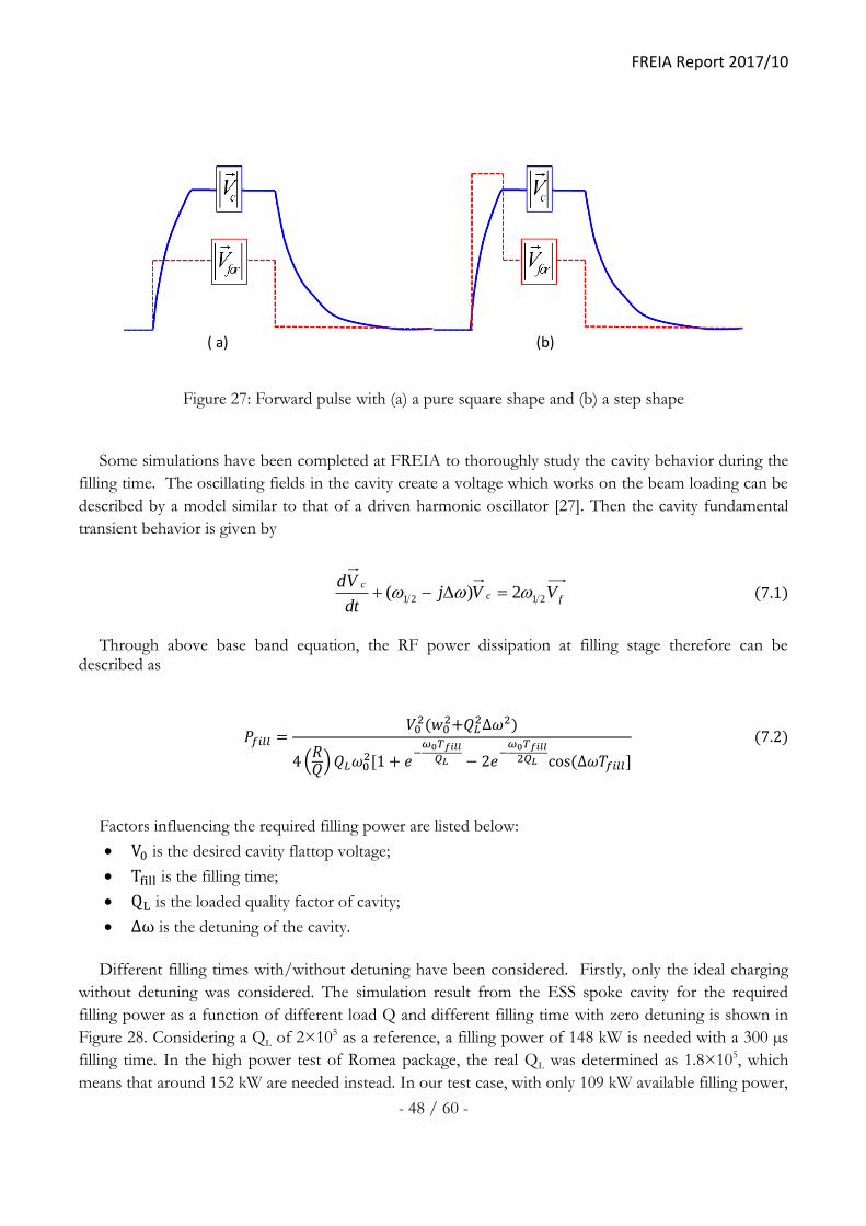
( a) (b)

Figure 27: Forward pulse with (a) a pure square shape and (b) a step shape

Some simulations have been completed at FREIA to thoroughly study the cavity behavior during the

filling time. The oscillating fields in the cavity create a voltage which works on the beam loading can be

described by a model similar to that of a driven harmonic oscillator [27]. Then the cavity fundamental

transient behavior is given by

fcc

VVjdt

Vd2121 2)( (7.1)

Through above base band equation, the RF power dissipation at filling stage therefore can be

described as

𝑃𝑓𝑖𝑙𝑙 =𝑉0

2(𝑤02+𝑄𝐿

2∆𝜔2)

4 (𝑅𝑄) 𝑄𝐿𝜔0

2[1 + 𝑒−

𝜔0𝑇𝑓𝑖𝑙𝑙

𝑄𝐿 − 2𝑒−

𝜔0𝑇𝑓𝑖𝑙𝑙

2𝑄𝐿 cos (∆𝜔𝑇𝑓𝑖𝑙𝑙]

(7.2)

Factors influencing the required filling power are listed below:

V0 is the desired cavity flattop voltage;

Tfill is the filling time;

QL is the loaded quality factor of cavity;

∆ω is the detuning of the cavity.

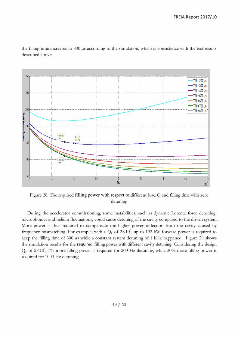
Different filling times with/without detuning have been considered. Firstly, only the ideal charging

without detuning was considered. The simulation result from the ESS spoke cavity for the required

filling power as a function of different load Q and different filling time with zero detuning is shown in

Figure 28. Considering a QL of 2×105 as a reference, a filling power of 148 kW is needed with a 300 µs

filling time. In the high power test of Romea package, the real QL was determined as 1.8×105, which

means that around 152 kW are needed instead. In our test case, with only 109 kW available filling power,


- 49 / 60 -

the filling time increases to 800 µs according to the simulation, which is consistence with the test results

described above.

Figure 28: The required filling power with respect to different load Q and filling time with zero

detuning

During the accelerator commissioning, some instabilities, such as dynamic Lorentz force detuning,

microphonics and helium fluctuations, could cause detuning of the cavity compared to the driven system.

More power is thus required to compensate the higher power reflection from the cavity caused by

frequency mismatching. For example, with a QL of 2×105, up to 192 kW forward power is required to

keep the filling time of 300 µs while a constant system detuning of 1 kHz happened. Figure 29 shows

the simulation results for the required filling power with different cavity detuning. Considering the design

QL of 2×105, 1% more filling power is required for 200 Hz detuning, while 30% more filling power is

required for 1000 Hz detuning.


- 50 / 60 -

Figure 29: The required filling power with different cavity detuning

The peak power of 400 kW, according to the power capacity of the DB Elettronica RF station tested

at FREIA, will lose some power on the RF distribution leading to the cryostat and only transfer about

350 kW to the FPC. In this case, the fastest filling time of the ESS spoke cavity calculated by Equation

(7.2) is therefore about 135 µs with the design QL of 2×105. Fortunately, with a fixed forward power of

350 kW, a 1 kHz detuning of the system does not affect the filling significantly. A simulation of the

filling time as a function of detuning with a fixed 350 kW forward power is shown is Figure 30. Here the

filling time has increased by only 7 us for a 1 kHz frequency mismatch.


- 51 / 60 -

Figure 30: filling time as a function of detuning with a fixed 350 kW forward power

According to the above simulation, two-step forward pulse profile can be applied to the ESS spoke

cavity in the high power test without beam. With a requirement of 300 µs filling time, a forward power

of 152 kW is needed during the charging stage followed by cutting down to 108 kW for maintaining a

gradient of 9 MV/m. The filling time can also be shortened to 135 µs by using the maximum forward

power of 350 kW. The comparison of these step pulse profiles is shown in Figure 31. The system

detuning usually varies during the filling stage in the real situation. By regulating a forward power from

152 kW to 350 W, the practical filling time is therefore in a range from 135 to 300 µs.

Figure 31: Examples of forward power profiles to ESS spoke cavity at high power test without beam for

(a) 300 us or (b) 135 us filling times.


- 52 / 60 -

Dynamic Lorentz force detuning 7.2.

The main source of distortion in a pulsed accelerator is the Lorentz force. In ESS operation, the cavity is

reloaded with a frequency of 14Hz. Due to the pulsed operation, the cavity wall is deformed by the

Lorentz force detuning (LFD) caused by the accelerating electromagnetic field and leads to an extra RF

power requirement. Since the LFD is repetitive and predictable, its behaviour has been measured by

monitoring and manipulating the complex signals from the cavity during the pulse using an FPGA-based

LabView program at FREIA. Measured signals, like forward voltage and transmitted voltage, are first

calibrated and normalized by using Equation (7.3). Figure 32 b) shows that the measured and calibrated

transmitted voltage match well both in magnitude and phase. Here the calibrated transmitted voltage is

calculated by using forward and reflected voltage from Figure 32 a), from which the coefficient C1 and

C2 is obtained. The calibrated cavity voltages therefore fulfill the baseband Equation (7.1) of a

superconducting cavity [28]. Here cVand fV

are the complex transmitted and forward voltage of the

cavity while 21 and are the instantaneous half bandwidth and detuning of the cavity respectively.

measff

measrmeasfc

VcV

VcVcV

,1

,2,1 (7.3)

The experimental result is shown in Figure 32 c), suggesting 400 Hz frequency shift at the

accelerating gradient of 9 MV/m @ 2.86 ms pulse length. The shift is comparable to the cavity

bandwidth. This result provides important input for the fast frequency compensation with a cold tuning

system in the future test. Also from the calculation by using the instantaneous half bandwidth 21 , a

loaded quality factor of 1.8×105 was obtained, which was consistent with the measurement with a vector

network analyzer.


- 53 / 60 -

Figure 32: a) shows the forward (black curve), reflected (red curve) and transmitted signal (green curve)

in the cavity during a pulse which collected by the FPGA board; b) shows a well agreement of both the

magnitude (green and blue) and phase (red and purple) information of the measured and calibrated

transmitted voltage; c) shows the LFD at 9 MV/m and d) shows the QL of the cavity calculated by the

state space equation.

Pressure sensitivity 7.3.

Helium pressure fluctuations inside the tank deform the cavity wall, which is one of the main sources of

cavity resonance frequency detuning. Measuring the frequency sensitivity as a function of helium

pressure provides information about the mechanical stability of the cavity. There are several ways to

carry out cavity mechanical stability measurements. One direct way is to measure the frequency shift as a

function of transient pressure. Another simple way is to check the resonant frequency shift during cool

down from 4.2 K to 2 K, where the helium pressure is reduced from roughly one atmosphere to 30

mbar.

a) b)

c) d)


- 54 / 60 -

Figure 33: Cavity frequency shift as a function of helium pressure from 20 to 40 mbar

In this test, by keeping both the inlet and the outlet valves close, the helium pressure in the 2K tank

subsequently increased due to the static heat load. By checking the cavity frequency as a function of

pressure from 20 to 40 mbar, as shown in Figure 33, a pressure sensitivity of +27 Hz/mbar was

measured. This result is in good agreement with the 28 kHz frequency shift found while reducing the

helium pressure from roughly one bar to 30 mbar. In this way, the frequency sensitivity can be calculated

by equation (7.4).

𝑓𝑟𝑒𝑞𝑢𝑒𝑛𝑐𝑦 𝑠𝑒𝑛𝑠𝑖𝑡𝑖𝑣𝑖𝑡𝑦 (𝐻𝑧 𝑚𝑏𝑎𝑟⁄ ) =𝑓(4.2 𝐾) − 𝑓(2 𝐾)

𝑝𝑟𝑒𝑠𝑠𝑢𝑟𝑒 (4.2 𝐾) − 𝑝𝑟𝑒𝑠𝑠𝑢𝑟𝑒 (2 𝐾) (7.4)

Note that the mechanical contraction of the cavity from 4K to 2K is very small, thus the frequency

shift caused by this temperature change can be ignored.

Because of different fabrication procedures, the frequency shift varies among cavities from different

manufacturers. Thus the pressure sensitivity measurement could be helpful for optimizing production

procedures.

Mechanical modes 7.4.

We studied the mechanical modes of the ESS spoke cavity by stimulating the cavity with forward

amplitude modulation provided by a gain-controller, based on NI FlexRIO FPGA and NI 5782R data

acquisition modules developed at FREIA. Meanwhile, the transmitted signal was monitored by a Rohde

& Schwarz (RTO 1024) oscilloscope with a built-in I/Q demodulation option. This is a convenient


- 55 / 60 -

method to determine the mechanical modes by modulating the radiation pressure at angular frequency in

order to excite one resonant mode only. To this end, one can drive the cavity in a long pulse mode at a

relatively high gradient V0, introduce a small periodic modulation of the cavity voltage and sweep the

modulation frequency. This will allow measuring the amplitude and phase of the cavity frequency

modulation as a function of the sweep frequency ω.

Several tests were performed at 20 mbar to find out the optimal parameters of the loop, for example,

the RF station from DB Elettronica was turned to CW mode which can provide a pulse longer than 4

ms, a driven pulse with 350 ms duration and a gradient of 1.6 MV/m was chosen for the balance of

coupler average power and measurement accuracy. A sweeping modulation frequency had a resolution

down to 3 Hz, which is depend on the measurement time, namely the pulse length. A voltage

modulation depth of 40% was set to start the modulation frequency, which will become lower while

increasing the modulation frequency. Subsequent off-line analysis of the demodulated signal revealed the

frequency shift as a function of time. The strength of the cavity package vibration at a given modulation

frequency was then obtained by taking the Fourier transform.

Table 13: The simulation result of dangerous mechanical modes given by IPN Orsay

N° Frequency Mode

1 & 2 212 Hz Beam tube on CTS side

3 & 4 265 Hz & 275 Hz Spoke bar/Helium vessel

5 & 6 285 Hz Coupled mode Cavity/Helium vessel

7 313 Hz Helium vessel

8 to 11 315 Hz to 365 Hz Coupled mode Cavity/Helium vessel

12 396 Hz beam tubes


- 56 / 60 -

Figure 34: Fit of mechanical modes of ESS spoke cavity

By sweeping the modulation frequency up to 800 Hz, the fit of the mechanical modes was studied

and is shown in Figure 34. Note that the slow tuner was in fixed position during the mechanical modes

measurement. Two major mechanical modes at 265 Hz and 343 Hz were found, which give similar

results when compared to IPN Orsay’s simulation (Table 13). These values will then be considered in

further LFD compensation development with the piezos.

Tuner sensitivity 7.5.

The cold tuning system (CTS) is attached to the spoke cavity to adjust its resonant frequency in order to

counteract the frequency detuning. The spoke CTS integrates two different functions: a slow tuning

capability over a wide frequency range by using a step motor and a fast tuning system by means of

piezoelectric actuators inserted in the mechanical system of the CTS [29].

The tuning sensitivity could be obtained by [30]

cavityCTS KKysensitivitcavitymmHzysensitivittuning

/1

11)/( (7.5)

Here, KCTS is the required CTS stiffness while the cavity stiffness Kcavity would be 20 kN/mm. The

behavior of the slow tuning system was studied at 20 mbar helium pressure at FREIA, as shown in

Figure 35. A tuning sensitivity of 150 KHz/mm @ 20 mbar was found.


- 57 / 60 -

Figure 35: Cavity frequency vs. motor position at 20 mbar

8. Production testing plan Due to a tight schedule, cavities Romea and Giulietta will go through an extra high pressure rinsing

(HPR) process and then will be installed in a prototype cryomodule with new fully conditioned FPCs at

IPN Orsay. FREIA will then prepare the acceptance testing of the spoke prototype crymodule. This is

the first prototype with two dressed spoke cavities that will be installed in the ESS linac. The main

difference between the coming cryomodule test and the individual cavity package test in HNOSS is that

two cavities will be installed in an ESS cryomodule prototype, each with its own magnetic shield

integrated with the cavity. Then a busy schedule will follow by testing another 13 spoke crymodules at

FREIA before delivering to ESS.

9. Summary The qualification of the cavity package with high power test represents an important verification before

the module assembly. The first spoke cavity assembled with all ancillary components was installed in

HNOSS and completed high power tests based on the self-exited loop at FREIA.


- 58 / 60 -

This cavity was operated at the pulse mode of 2.86 ms duration and 14Hz repetition rate. Maximum

power of 120 kW was reached, which successfully built up a field of 9 MV/m. The quality factor of the

Romea cavity package was determined 1.4×109 at low field and 2.8×108 at 9 MV/m. A high radiation of

6 mSv/h and a high heat load of about 12 W was observed when the cavity package was operating at its

design field. The radiation did not seem to reduce significantly with accumulated running hours. Possible

reasons and solutions are under study. Considerations are focusing on the following five hypotheses: a

contaminated FPC, particles generated during conditioning cryopumped on the cavity’s surface, FPC is

not fully conditioned, a bigger impact on heat load than expected from the FPC into the cavity or a

combination of all these. A warm up after cavity package conditioning up to 40 K would be highly

recommended to improve the cavity performance as well as to reduce the system’s dynamic heat load.

Also, installing one extra pump at the coupler side would significantly improve the pumping efficiency

and would be very helpful in avoiding contamination in the cavity wall.

According to the simulation, two-step forward pulse profile can be applied to the ESS spoke cavity in

the high power test without beam. With a requirement of 300 µs filling time, a forward power of 152 kW

is needed during the charging stage followed by cutting down to 108 kW for maintaining a gradient of 9

MV/m. The filling time can also be shortened to 135 µs by using the maximum forward power of 350

kW. The system detuning usually varies during the filling stage in the real situation. By regulating a

forward power from 152 kW to 350 W, the practical filling time is therefore in a range from 135 to 300

µs.

The key frequencies of Romea at three different temperatures were under check, from which the

frequency increment due to cryo-constriction was about 500 kHz from 300 K to 4 K, while a frequency

decreasing of 27 kHz happened from 4 K to 2 K since the helium pressure decrease from 1 atmosphere

to 30 mbar. The dynamic Lorentz detuning was studied by a signal generator driven system without

frequency feedback. A frequency shift of about 400 Hz was determined during the pulse flat top and the

two mechanical modes of the cavity package, found at 343 Hz and 265 Hz, show a good agreement with

simulations.


- 59 / 60 -

References [1] Steve Peggs, Conceptual design report, 2012.

[2] P. Duchesne et al., “Design of the 352 MHz, Beta 0.50, double-spoke cavity for ESS”, SRF 2013,

FRIOC01.

[3] R. Ruber et al., “The New FREIA Laboratory for Accelerator Development”, Proceedings

IPAC'14, Dresden, Germany (2014) THPRO077.

[4] Roger Ruber et al., “Uppsala test facility project plan. Uppsala University”, FREIA report

062013/3.

[5] Han Li, et,al. “Test Characterization of Superconducting Spoke Cavities at Uppsala university”,

SRF2015,TUP083.

[6] “CNRS and ESS Advance a New Standard for Linac Design”, Last modified September 30,

2015.

https://europeanspallationsource.se/sites/default/files/spoke_cavities_wp4_pdf_0.pdf.

[7] “Spoke RF”, Accessed January 20,2016. https://europeanspallationsource.se/spoke-srf.

[8] P. Duchesne et al., “Design of the 352 MHz, Beta 0.50, double-spoke cavity for ESS”, SRF 2013,

FRIOC01.

[9] Guillaume OLRY, “Spoke Cryomodules (WP4)”, Last modified April 21, 2015.

https://indico.esss.lu.se/event/316/contribution/17/material/1/1.pdf.

[10] R. Santiago Kern et al., “The HNOSS horizontal cryostat and helium liquefaction plant at

FREIA”, IPAC 2014, WEPRI110.

[11] Santiago Kern R. 2017, “Setting for Run 8 (Romea with FPC and CTS) ”, FREIA Memo 2017-

01-M.

[12] Jean Delayen. “Self-exited loop”, Jefferson lab LLRF workshop, 2001.

[13] https://europeanspallationsource.se/article/stage-set-ess-linac-test-uppsala

[14] A. J .Johansson et al., “ LLRF System for ESS Linac”, System description,2016.

[15] E. Rampnoux. “ RF conditioning test stand”, presentation of Uppsala University-IPN Orasy

meeting, December 1st, 2016.

[16] E. Rampnoux, “Parametres_Prog_Cdt_Cpl_FREIA_v1”, internal document.

[17] H. Li et al., “ESS Spoke Cavity Conditioning at FREIA”, IPAC 2017, MOPVA094

[18] R. Santiago Kern, “Synopsis for Run 8 (Romea with FPC and CTS) ”, FREIA Memo 2017-02-

M.

https://europeanspallationsource.se/sites/default/files/spoke_cavities_wp4_pdf_0.pdf

https://europeanspallationsource.se/article/stage-set-ess-linac-test-uppsala


- 60 / 60 -

[19] T. powers., “Theory and practice of cavity RF test system”, 12th international workshop on RF

superconductivity.

[20] R. E.Honlg and H.O.Hook. “Vapor pressure data for some common gases”, RCA Review

21,360(1960)

[21] Private conversation with Younguk Sohn at PSL2 and Keihan Tavakoli at SOLEIL

[22] Santiago Kern R. 2017, “Synopsis for Run 8 (Romea with FPC and CTS) ”, FREIA Memo 2017-

02-M.

[23] Philip R. Bevington, “Data Reduction and Error Analysis for Physical Sciences”, 3rd ed.,

McGrw-Hill, 2002(338s)

[24] N1911A/N1912A P-Series Power Meters and N1921A/N1922A Wideband Power Sensors data

sheet

[25] William H. Press et al., “ Numerical recipes in Fortran 77” ,2nd ed., 1997(1574s)

[26] Steve Peggs, ESS technical design report,2013, 321.

[27] T.P.Wangler, RF Linear Accelerators, Wiley-VCH, New York, 2011

[28] T. Schilcher. Vector Sum Control of Pulsed Accelerating Fields in Lorentz Force Detuned

Superconducting Cavities. Ph. D. Thesis of DESY, 1998

[29] N. Gandolfo et al., “Reynet Deformation tuner design for a double Spoke cavity”, SRF 2013,

THP078.

[30] Steve Peggs, ESS technical design report, 2013, 321.

Documents

First High Power Test of the ESS Double Spoke Cavity1162798/... · 2017-12-05 · FREIA Report 2017/10 - 6 / 60 - of overall power coupler conditioning. The object of this test thus