Firm Value and Managerial Incentives: A StochasticFrontier Approach1

Michel A. Habib2 Alexander P. Ljungqvist3

March 15, 2000

1We thank Tim Coelli for his continued help throughout this project; seminar participantsat the universities of Bristol, Mannheim, Oxford, Vienna, and Warwick for helpful comments;Scott de Carlo and Cecily Fluke from Forbes for kindly providing us with part of the data; andDavid Stolin, Deborah Lisburne and Ronnie Barnes for excellent research assistance. We gratefullyacknowledge funding from the European Union, Training and Mobility of Researchers grant no.ERBFMRXCT960054 (Habib and Ljungqvist) and an Oxford Faculty Research Grant (Ljungqvist).

2London Business School, Sussex Place, Regent’s Park, London, NW1 4SA. Tel: (0171) 262-5050, fax: (0171) 724-3317, e-mail: mhabib@london.edu.

3From July 2000: Stern School of Business, New York University; and CEPR. Cur-rently visiting London Business School. Tel: (0171) 262-5050, fax: (0171) 724-3317, e-mail:aljungqvist@london.edu.

Abstract

We examine the relation between firm value and managerial incentives in a sample of 1,487U.S. firms in 1992-1997, for which the separation of ownership and control is complete.Unlike previous studies, we employ a measure of relative performance which compares afirm’s actual Tobin’s Q to the Q∗ of a hypothetical fully-efficient firm having the sameinputs and characteristics as the original firm. We find that the Q of the average firm inour sample is around 10% lower than its Q∗, equivalent to a $1,340 million reduction inits potential market value. We investigate what causes firms to fail to reach their Q∗ andfind that our firms are more efficient, the higher are CEO stockholdings and optionholdingsand the more sensitive are CEO options to firm risk. We also show that boards respond toinefficiency by subsequently strengthening incentives or replacing inefficient CEOs.

1 Introduction

The separation of ownership and control has been a long-standing concern in finance. In1932, Berle and Means predicted that the increasing professionalization of managementwould lead to firms being run for the benefit of their managers rather than that of theirowners. In 1976, Jensen and Meckling used a principal-agent framework to analyze the con-flict of interest between managers and shareholders. The subsequent literature has analyzeddifferent mechanisms that serve to align the interests of managers with those of shareholders.Examples include the threat of hostile takeovers, career concerns, and the structure of man-agerial compensation contracts. A rich empirical literature has investigated the efficacy ofthese mechanisms. For example, Jensen and Murphy (1990) examined the relation betweenmanagerial pay and firm performance. They argued that this relation was too small to beeffectual.1

A rather smaller literature has attempted to test directly what has come to be calledthe Berle and Means hypothesis: managers fail to maximize firm value where they arenot themselves significant shareholders. The empirical evidence on this point is mixed.Using data from the early 1930s, the period in which Berle and Means put forward theirhypothesis, Stigler and Friedland (1983) found no evidence that manager-controlled firmswere less profitable than their shareholder-controlled counterparts. Using more recent data,Demsetz and Lehn (1985) found no relation between firm performance, as measured byreturn on assets, and ownership concentration. In contrast, both Mørck, Shleifer, and Vishny(1988) and McConnell and Servaes (1990) found a significant relation between firm value, asmeasured by Tobin’s Q, and managerial stockholdings.

The findings of Mørck, Shleifer, and Vishny (1988) and McConnell and Servaes (1990)have recently been questioned by Agrawal and Knoeber (1996) and Himmelberg, Hubbard,and Palia (1999), who explicitly adjust their test designs for the endogeneity of managerialstockholdings to firm value. Using simultaneous equations (Agrawal and Knoeber) and firmfixed effects (Himmelberg, Hubbard, and Palia), they find no relation between firm value andmanagerial stockholdings and conclude that managerial stockholdings are chosen optimally.

Our paper continues this line of enquiry in that it explores the link between firm valueand managerial incentives in a panel of 1,487 publicly traded U.S. companies over the years1992 to 1997. Its contribution is three-fold. First, we employ an econometric frameworkthat specifically tests whether companies are run efficiently. Unlike previous studies, whichlook at a firm’s actual Q, we compute the Q∗ of a hypothetical fully-efficient firm havingthe same inputs and characteristics as the original firm. We find that the Q of the averagefirm in our sample is around 10% lower than its Q∗. Translated into dollars, this means thatthe average firm could increase its market value by $1,340 million were it to become fullyefficient. This suggests the presence of systematic inefficiency across our firms, consistentwith the Berle and Means hypothesis.

Our estimates of Q∗ are based on an econometric technique called stochastic frontieranalysis.2 Consider a set of firms, each of which has access to the same production inputs.

1For an alternative view, see Aggarwal and Samwick (1998), Garen (1994), Hall and Liebman (1998),Haubrich (1993), John and John (1993) and others. See Murphy (1998) for a review.

2Stochastic frontier analysis was pioneered by Aigner, Lovell, and Schmidt (1977) and Meeusen and vanden Broeck (1977) and is widely used in economic studies of productivity and technical efficiency. Two

1

Clearly we would not expect all firms to be equally efficient, for even given the same inputs,the different managers may make different production, investment and strategic decisions,in response to the financial and other incentives they face, and on the basis of their ability,disutility of effort and risk aversion. Some firms will therefore have higher Tobin’s Qs thanothers. The firms with the highest Qs are the most efficient and thus define points on afrontier, analogous to the microeconomic concept of a production possibility frontier. It isin the nature of a frontier that firms can only lie on the frontier or below it, but never aboveit. Efficiency then corresponds to all firms being on the frontier, given their inputs, whereasinefficiency corresponds to a significant fraction of firms lying below the frontier. There are nofirms above the (true) frontier, though the technique allows for random noise in locating thefrontier empirically. Estimating the frontier requires a comprehensive set of ‘input’ variablesto control for firms’ characteristics. We draw on the literature, and especially Himmelberg,Hubbard, and Palia (1999), in our search for relevant input variables.

Our second contribution is to investigate what causes firms to fail to reach their Q∗. Sincewe have already accounted for random influences on value (such as bad luck or windfalls),we assume inefficiency is caused by conflicts of interest, which can however be mitigatedvia incentive schemes. Specifically, if incentives matter, we expect firms to be closer totheir potential, the better designed their incentive schemes. We distinguish between internalincentives (which are at least partly controllable by the board of directors) and externalincentives (which are largely determined by the market). In investigating the efficacy ofinternal incentives empirically, we not only look at managerial stockholdings but also atmanagerial option plans.3 Including options is appropriate for three reasons. First, Murphy(1998) documents that stock options have become increasingly widespread since the 1980s,yet their effect on firm value has not hitherto been explored. Second, a small but growingliterature documents the importance of options as managerial incentives in specific cases.4

Berger and Ofek (1999), for example, show that options, but not stocks, induce managersto refocus diversified companies voluntarily, thus reversing value-destroying diversification.Third, stockholdings and optionholdings are interdependent: Ofek and Yermack (2000) showthat managers tend to reduce their direct stockholdings following option awards. Controllingfor one without controlling for the other may thus bias empirical results. Lambert, Larcker,and Verrecchia (1991) argue that the value of an option alone is unlikely to capture all itsincentive effects, due to the convexity of its payoff function. Following this argument, wedistinguish between the effort-inducing effect of managerial optionholdings and their effecton managers’ choice of project risk. As noted by Guay (1999), the former can be measuredby the number of options the manager holds, whereas the latter can be measured by thesensitivity of option value to risk, or vega. Guay shows that vega is positively relatedto companies’ investment opportunities which is consistent with boards seeking to provide

applications in finance are studies of banking efficiency (Berger and Humphrey, 1997) and a recent articleon pricing efficiency in the IPO market (Hunt-McCool, Koh, and Francis, 1996).

3We also investigate whether greater use of debt improves efficiency, as in Jensen’s (1986) free cash flowhypothesis, but find no significant effect.

4There is a larger literature that investigates the contribution of options to pay-performance sensitivities(as in Jensen and Murphy, 1990) and the relative mix of options, stock, and cash compensation as a functionof companies’ investment opportunities set. See, for instance, Hall and Liebman (1998) and Bryan, Hwangand Lilien (2000). However, this literature does not address how the use of options affects firm value.

2

incentives to invest in risky projects.In addition to these internal incentives, we investigate the efficiency effects of two possible

external incentives: capital market pressure (the probability of delisting in each industry)and product market pressure (the degree of competition in the each firm’s primary line ofbusiness). Product market pressure has an ambiguous effect on value a priori. On the onehand, Schmidt (1997) and others have argued there is more scope for managerial slack in lesscompetitive markets, resulting in lower Tobin’s Qs. On the other, firms in less competitivemarkets might earn higher economic rents and thus have higher Tobin’s Qs.

We find that firms in our sample are more efficient, the better their internal and exter-nal incentive structures. Consistent with the Berle and Means hypothesis and the resultsof Mørck, Shleifer, and Vishny (1988) and McConnell and Servaes (1990), we find that in-efficiency is greater, the lower are CEO stockholdings. Interestingly, the same is true foroptionholdings: contrary to popular belief,5 CEOs (in our sample) are not given enoughoptions. This is particularly true for large companies, where suboptimal option awards ap-pear to be the only determinant of managerial inefficiency. This may qualify the findings ofHimmelberg, Hubbard, and Palia (1999), who do not include options in their tests. We alsofind that inefficiency decreases in option vega, so CEOs’ options are not sufficiently sensitiveto risk. These results confirm that internal incentive schemes do work in the intended way,but that not every firm provides optimal incentives at every point in time. Economically,the effects are large: all else equal, a one standard deviation increase in stockholdings fromthe mean would increase market value by $1,198 million on average, while similar increasesin optionholdings and vega would increase market value by $775 million and $352 million,respectively.

To illustrate the SFA approach, consider two sample companies which are comparable intheir input variables and firm characteristics: Mueller Industries Inc (SIC code 335 - Metalfabricators) and Novacare Inc (SIC code 809 - Long-term health care). In 1994, the twocompanies had similar levels of sales, firm-specific risk, soft and hard capital spending, andleverage. But whereas Novacare’s Q equalled its Q∗, Mueller Industries’ was 21% below.This difference in efficiency is largely due to differences in incentives: Mueller’s CEO hadnegligible stockholdings (0.008% of outstanding equity vs. 5.1%), modest optionholdings(1.5% vs. 4.7%) and much lower vega.

With regards to external incentives, we show that companies in more competitive indus-tries are more efficient, which suggests that the incentive effect of competition dominatesthe rent effect of concentration. We also find evidence that capital market pressure has anambiguous effect on efficiency. Firms appear to be more inefficient, the greater the proba-bility of delisting, though the economic magnitude of this surprising result is small for allfirms except utilities.

Our findings regarding inefficiency and its causes are robust to partitioning the sampleby size and industry, as well as to standard outlier tests and alternative measures of theeffort incentives provided by stocks and options (Baker and Hall, 1999).

Our third contribution is to answer a natural question raised by our empirical findings:given that there appears to be systematic inefficiency in our sample and that better in-centives are linked to lower inefficiency, do boards respond to inefficiency by subsequently

5See for instance “The trouble with share options”, The Economist, August 7th, 1999.

3

adjusting internal incentives? The answer is yes. We show that boards are more likely toaward restricted stock and options, and that such awards are larger, following periods of lowefficiency. We find that boards make CEOs’ options more sensitive to risk the greater pastinefficiency. Boards also appear to cut cash salaries in response to poor efficiency, changingthe cash compensation mix away from fixed salaries towards bonuses. Finally, boards aremore likely to replace a CEO aged 60 or under, the worse past efficiency. In other words,boards react to managerial inefficiency by strengthening incentives or replacing CEOs. Wealso show that it is the firms whose incentives are strengthened the most that increase effi-ciency the most over time.

Do boards react to relative efficiency or to absolute firm value? To check, we replace ourmeasure of efficiency, the distance between Q and Q∗, by Q alone. Interestingly, Q aloneis a far less effective predictor of subsequent board actions than is the distance between Qand Q∗. This suggests that boards react to firms not achieving their full-potential Q∗ ratherthan to absolute Q.

One potential problem in testing the Berle and Means hypothesis is that incentives maynot only affect efficiency, but efficiency may also affect incentives. Himmelberg, Hubbard,and Palia (1999), henceforth HHP, argue persuasively that the inclusion of fixed firm effectswill help control for this endogeneity of managerial incentives, insofar as endogeneity givesrise to unobserved but time-invariant heterogeneity across firms. To borrow one of theirillustrations, consider two identical firms, one of which has access to more effective monitoringtechnology which reduces its optimal level of managerial ownership. If the combination ofmanagerial ownership incentives and effective monitoring achieves a higher Tobin’s Q but weare unable to control for differences in monitoring technology, we would spuriously concludethat companies are more efficient, the lower managerial ownership. As HHP show, the useof repeated observations on the same set of firms (that is, panel data) allows us to removeunobserved factors such as differences in monitoring technology via fixed effects, as longas these unobserved factors do not change over time. We therefore include fixed effectsin our stochastic frontier regression, as well as in our model of how boards react to pastinefficiency. Like HHP, we find that unobserved firm effects are significant and thereforeneed to be controlled for.

As an alternative to mitigating endogeneity bias by way of fixed effects, we also investigatean instrumental-variables approach and find that our results are little changed. However,since good instruments are notoriously hard to find, we view the IV results as indicativeonly.

The paper proceeds as follows. Section 2 outlines our empirical approach, including abrief explanation of stochastic frontier analysis, and specifies our empirical model. Section 3describes the data and Sections 4 and 5 present the empirical results regarding inefficiencyand board reaction, respectively. Finally, Section 6 concludes.

4

2 Empirical approach

2.1 Stochastic frontier analysis

A conventional regression of Q on managerial stockholdings and the appropriate controlvariables results in the estimation of an ‘average’ function for Q. But a study of efficiencyrequires the estimation not of the average function for Q, but of the ‘frontier’ function for Q;that is the function that specifies the highest Q that can be achieved for a given set of inputssuch as R&D, investment, managerial ability, etc. Stochastic frontier analysis allows such afrontier function to be estimated, by supplementing the conventional, two-sided, zero-meanregression error term with a one-sided error term. This second term is zero for the efficientfirms that achieve the highest Q, but strictly positive for those firms that are inefficient andtherefore fail to achieve as high a Q as can be achieved given their inputs. In analogy withconventional panel-data notation, we can express Q as a function of a set of explanatoryvariables X, firm-specific but unobservable factors η assumed to be time-invariant, and anerror term ε:

Qit = βXit + ηi + εit (1)

where i = 1, ..., N and t = 1, ..., Ti.It is the special form of the error term εit that enables us to detect possible departures

from efficiency. Specifically, εit is composed of two terms: εit = vit−uit. The two-sided errorterm vit denotes the zero-mean, symmetric error component that is found in conventionalregression equations. It allows for estimation error in locating the frontier itself, thus pre-venting the frontier from being set by outliers. The one-sided error term uit > 0 permits theidentification of the frontier, by making possible the distinction between firms that are onthe frontier (uit = 0) and firms that are strictly below the frontier (uit > 0). Of course, if allfirms were on the frontier, then uit = 0 and Qit = Q∗

it ∀i, t: all firms would be efficient andwould achieve the highest feasible Q∗ given their inputs. In that case, SFA would reduce toa conventional regression, for the average function and the frontier function would then beidentical.

A measure of a firm’s inefficiency or relative performance is uit. Using this, we can com-pute firm i’s predicted efficiency in year t as the ratio of its realized Q to the correspondingQ∗ ≡ Q+u if it was fully efficient: PEit = E(Qit|uit,Xit)

E(Q∗it|uit=0,Xit)

; for further details, see Battese and

Coelli (1988). Predicted efficiencies lie between 0 and 1, with 1 being the frontier. If firmi’s predicted efficiency is 0.85, then this implies that it achieves 85% of the performance ofa fully efficient firm having comparable inputs.

2.2 Including fixed effects

Least-squares or standard SFA estimation of equation (1) will lead to biased coefficientestimates due to the presence of the unobserved ηi factors. If we have repeated observationsof companies across time, we can estimate equation (1) consistently by either i) including Nfirm dummies or ii) transforming the regression into one where the variables are expressedas deviations from their within-group means. The first method is impracticable where N is

5

large, as it is in our case, due to the size of the matrix that must be inverted. The secondgives:

Qit −Qi = β(Xit −X i

)+ vit − vi − (uit − ui) (2)

where Qi ≡ 1Ti

Ti∑t=1

Qit and X i, vi, and ui are similarly defined. This transformation cannot

be estimated by SFA, however, as uit − ui may be negative for some i and t. In order tomake the use of SFA possible, we add back the ‘grand mean’ of each variable to (2):6

Qit −Qi + Q = β(Xit −X i + X

)+ η + vit − vi + v − (uit − ui + u) (3)

where Q ≡ 1N

N∑i=1

Qi = 1N

N∑i=1

(1Ti

Ti∑t=1

Qit

)denotes the grand mean of Qit and X, η, v, and u are

similarly defined. The advantage of regression (3) over regression (2) is that uit− ui + u > 0under the assumption that |uit − ui| � u. Regression (3) can therefore be estimated by SFA.

Note that the transformations (2) and (3) leave the parameters of interest β unaffected.

2.3 Testing for and explaining departures from efficiency

We test for efficiency by assessing the significance of the likelihood gain from imposing theadditional one-sided error term (Stevenson, 1980; Battese and Coelli, 1992). If uit = 0 ∀i, tthen the likelihood of the SFA specification will be the same as the least-squares likelihood.But if uit > 0 for sufficiently many i and t, then the SFA specification will lead to a likelihoodgain. This likelihood-ratio test corresponds to testing whether the average and the frontierfunctions are identical.

A rejection of the null hypothesis of efficiency naturally raises the question of what causesinefficiency. As inefficiency is measured by the distance from the frontier u, a second regres-sion of u on suspected causes of inefficiency can shed light on the reasons for the failure toperform efficiently and their relative importance. However, as noted by Reifschneider andStevenson (1991), this two-stage procedure is less statistically efficient than joint maximumlikelihood estimation of the frontier function and the distance from the frontier. In imple-menting the joint MLE, Reifschneider and Stevenson (1991) and Battese and Coelli (1995)decompose the one-sided error term u into two components, an explained component andan unexplained component:

uit = δZit + ζ i + wit (4)

where Zit is a set of incentive variables and wit > −δZit − ζ i denotes the unexplainedcomponent of uit. We allow for the presence of unobserved but time-invariant factors ζ i,such as managerial ability or risk aversion. We can remove the ζ i by applying the sametransformation to Zit and wit as we previously did to equation (1). We thus obtain:

Qit −Qi + Q = β(Xit −X i + X

)+ η + vit − vi + v

−δ(Zit − Zi + Z

)− ζ − (wit − wi + w) (5)

6We use the term ‘grand mean’ to refer to the time series and cross section mean of a variable.

6

For the purposes of estimating the MLE, we assume vit−vi+v ∼ N (0, σ2v) and wit−wi+w is

the truncation of the normal distribution N (0, σ2) at −δ(Zit − Zi + Z

)− ζ: wit−wi +w >

−δ(Zit − Zi + Z

)− ζ.

We refer to equation (5) as the firm fixed effects SFA specification. Note that the ineffi-ciencies uit and their determinants Zit are allowed to vary over time. The specification cantherefore accommodate changes in the incentives given to CEOs.

A measure of our ability to explain the determinants of inefficiency — the appropriatenessof our choice of Z variables — is the variance of the transformed residual error term wit −wi + w. The better we are able to explain departures from the frontier u, the lower will bethe unexplained variance. A statistical test of the validity of our Z variables can then be

based on γ ≡ σ2w

σ2v+σ2

w∈ [0, 1], that is the ratio of the unexplained error and the total error

of the regression (Aigner, Lovell, and Schmidt, 1977). γ will be zero if our Z variables fullyaccount for departures from the frontier.

2.4 SFA versus least-squares regressions

SFA allows us to ask two related questions: i) do firms perform efficiently and ii) if not,does the degree of inefficiency depend on suboptimal incentives? Previous papers dealingwith the Berle-Means hypothesis have asked a somewhat different question, namely whetherperformance (usually Tobin’s Q) depends on managerial ownership, m. To test whethermanagerial ownership is chosen optimally, these papers view the coefficient of m as anestimate of the partial derivative of Q with respect to m, which at the optimum mustbe zero. A significantly positive coefficient of m is interpreted as consistent with inefficiency:firm performance could be further increased if managerial ownership were increased. Asignificantly negative coefficient is interpreted as managers owning ‘too much’ of the firm,possibly indicating entrenchment. And finally, a zero coefficient is taken to indicate optimalmanagerial ownership.

We argue on economic and econometric grounds that this is a weak test of the Berle-Means hypothesis. Economically, it suffers from its narrow focus: even if the coefficient onm is zero, as in HHP and Agrawal and Knoeber (1996), there is no guarantee that CEOs aremaximizing performance. Essentially, a zero slope coefficient on m is not a sufficient statisticfor efficient performance when there are substitutes and complements to equity incentivesthat boards could use to incentivize CEOs. For instance, HHP and Agrawal and Knoeberreadily admit that their research design leaves open the possibility that companies may havechosen (say) m optimally, but are inefficient in their use of (say) options. (This, incidentally,is precisely what we find amongst the largest firms in our dataset.) This implies that testsbased on regression coefficients being zero will only amount to tests of efficient performanceif we as econometricians start with the complete and comprehensive set of incentive tools.

Stochastic frontier analysis does not suffer from the need to be comprehensive, because itproceeds by first establishing whether a significant fraction of firms are inefficient and thentesting how the degree of inefficiency is related to firm-by-firm differences in the incentivevariables for which data is available: managerial ownership, use of options, board monitoring,pressure from capital, labor or product markets, and so on. This allows us to separate the

7

test of efficiency from the test of the determinants of inefficiency: if certain firms are belowthe frontier, they are inefficient for whatever reason(s), some or all of which we may or maynot be able to capture with our choice of incentive variables.

Econometrically, a test for optimality by means of a zero slope coefficient on m is biasedagainst rejecting the null hypothesis of optimality precisely when the null is false. To seethe economic intuition for our claim, recall that economic inefficiency implies asymmetry:efficient firms achieve the frontier Q∗, inefficient firms perform below the frontier, and nofirm performs above the frontier. This asymmetry has consequences for the error structurein empirical tests. Conditional on a set of control variables, the residuals of a regressionwith Tobin’s Q as its dependent variable have a skewed distribution. The skewness in theresiduals results in inefficient estimates when least-squares or similar techniques are usedand reduces the power of the zero-coefficient test for optimality.7 It is only when all firmsare on the frontier and therefore efficient that the residuals will be well-behaved, allowingthe true null of optimality to be correctly accepted. SFA adjusts for skewness by introducingthe one-sided error term to capture potential departures from the frontier. In the presence ofeconomic inefficiency, SFA will therefore yield more (statistically) efficient standard errors.

2.5 The empirical model

To implement the stochastic frontier approach, we need to specify the relevant X (input andfirm characteristics) and Z (incentive) variables.8 Our preferred specification includes manyX variables that have been used extensively in previous analyses of Tobin’s Q:

Qit = β1 ln(−

salesit) + β2 ln(+

salesit)2 + β3

−SIGMA1it

+β4

+

R&Dit

Kit

+β5

+

ADVit

Kit

+β6

+

CAPEXit

Kit

+β7

+

Yit

salesit

+β8

?

Kit

salesit

+β9

?

leverageit +β10

−Rit +β11

+

growthit

+year controls + missing-value dummies + ηi + εit (6)

where we have indicated the signs we expect using +, – and ? above the variables. Weinclude log sales and its square as controls for firm size, partly because smaller firms typi-cally have larger Qs, and partly because some of the Z variables (for instance, managerialownership) are size-dependent. SIGMA1 is a measure of firm-specific risk. Ceteris paribus,we expect riskier firms to have lower Qs since the trade-off between the CEO’s portfoliodiversification and incentives sustains lower optimal managerial stock- and optionholdingsthan in less risky firms. ‘Soft’ spending on research and development (R&D) and advertis-ing (ADV ), and ‘hard’ spending on capital formation (CAPEX), normalized by the capitalstock K, are expected to covary positively with Q. The operating margin Y

salesis a measure

7See Greene (1997), pp. 309-310.8Alternatively, one could leave the choice of X and Z variables unrestricted a priori (i.e. allow any

variable to be included both amongst the X and the Z), and choose whichever specification has the highestlog-likelihood. We prefer to frame the exposition in terms of input (X) and incentive (Z) variables, thoughwe did perform unrestricted specification searches.

8

of profitability and therefore, possibly, market power and should thus be positively relatedto Q. K

salescontrols for the relative importance of tangible capital in the firm’s production

technology. In a Modigliani-Miller world, leverage should not affect capital structure. How-ever, if tax shields are valuable or debt reduces agency problems as in Jensen’s (1986) freecash flow hypothesis, Tobin’s Q should increase in leverage. On the other hand, leveragecould proxy for difficult-to-measure intangible assets such as intellectual property, customerloyalty, or human capital: firms which are more reliant on intangible assets are likely to havelower leverage and possibly higher Qs. The net effect is therefore ambiguous. We includethe cost of capital R to account for the lower market value accorded a riskier stream ofcash flows: the numerator of Tobin’s Q is the market value of the firm, which is obtainedby discounting future cash flows at the firm’s cost of capital. Declining industries have fewgrowth opportunities and therefore low Tobin’s Q, which we attempt to control for by in-cluding contemporaneous industry growth rates. We allow the frontier to shift over timeby including year dummies. Finally, HHP suggest to deal with missing data by setting themissing values of the variable in question to zero and including a dummy which equals 1when data is missing, and zero otherwise. This avoids having to drop firm-years where datais missing. In our sample, some values of R&D, ADV , CAPEX, and SIGMA1 are missing,so we include three (4-1) dummies.

With the exception of leverage, R, and growth, our set of X variables is identical toHHP’s. HHP also include managerial stock ownership, but in our notation, this is a Zvariable. Our complete set of Z variables is:

uit = δZit + ζ i + wit

= δ1stockholdingsit + δ2stockholdings2it

+δ3optionholdingsit + δ4optionholdings2it

+δ5vegait + δ6capital market pressureit

+δ7product market pressureit + ζ i + wit (7)

The first five variables are designed to capture ‘internal incentives’ which are at least in partunder the board’s control. CEO stockholdings is the fraction of the firm the CEO owns viavested or restricted stock including beneficial holdings. Following Baker and Hall (1999), wemeasure the effort-incentives of managerial optionholdings as the product of the delta of theoptions and the fraction of firm equity which managers would acquire if they were to exercisethe options. This serves to make what are in effect potential managerial stockholdingscomparable to actual managerial stockholdings in their incentive effects.9 The total incentiveeffect of managerial ownership is the sum of the slope of managerial stockholdings and theslope of managerial optionholdings.10 As in previous studies, we include squared terms forstock (and option-) holdings to allow for non-linearities in their relationship with Tobin’s Q.

9See Baker and Hall (1999) for a formal analysis.10An alternative measure of the effort incentives of options multiplies our measure by the market value

of the firm’s equity. As noted by Baker and Hall (1999), ours is the proper incentive measure if managerialeffort is additive, in the sense of being invariant to firm size. The second measure is appropriate if managerialeffort is multiplicative and proportional to firm size. Murphy (1998) argues for the primacy of the additivemeasure. Our empirical results are wholly unaffected if we use the multiplicative measure instead.

9

To capture the extent to which managerial options influence choice of project risk we computeoption vegas, which measure the sensitivity of option value to a small change in volatility.Guay (1999) documents a positive relationship between vega and investment opportunities,which he interprets as ‘managers receiving incentives to invest in risky projects when thepotential loss from underinvestment in valuable risk-increasing projects is greatest.’

The last two variables are based on external incentives. Capital market pressure is acombined measure of the risk of bankruptcy and takeover, both of which should act todiscipline the CEO (Stulz, 1990 and Scharfstein, 1988). Product market pressure, a measureof the degree of product market competition, should discipline the CEO in similar ways tocapital market pressure (Schmidt, 1997).

Our empirical model does not (for lack of data) include every conceivable incentive vari-able in our attempt to find the determinants of inefficiency. Fortunately, as we indicatedearlier, stochastic frontier analysis does not require a complete empirical model to test forefficiency. So to the extent that our incentive variable set is incomplete, we only reduce ourability to explain departures from the frontier, not our ability to test for efficiency per se.In practice, our choice of incentive variables seems to account for most of the inefficiency wefind, except amongst financial firms.

3 The data

3.1 Data and sources

Our data set is derived from the October 1998 version of Standard & Poor’s ExecuComp.ExecuComp covers the 1,500 firms in the “S&P Super Composite Index,” consisting of the500 S&P 500, the 400 MidCap and the 600 SmallCap index firms, beginning in 1992. Weverify that firms which drop out of the indices are retained in the data set unless theycease to be listed, thus minimizing survivorship bias.11 As Standard & Poor’s change thecompositions of their indices, new firms are added to ExecuComp. In the October 1998version that we use, there are a total of 1,827 firms. Since being included in an index couldbe a sign of ‘success,’ using the whole universe of ExecuComp firms available in the October1998 version would over-represent ‘successful’ firms. We therefore limit our analysis to the1,500 original 1992 panel firms. Of these, we exclude twelve firms with dual CEOs and onefirm for which no Compustat data was available. This leaves a total sample of 1,487 firms.

The panel runs from 1992 to 1997 and consists of a total of 8,087 firm-years. This is 835short of the theoretical maximum of 1,487 firms × 6 years. There are two reasons why thepanel is unbalanced: attrition and missing data. 216 of the 1,487 companies delist prior to1997, resulting in a loss of 464 firm-years (an attrition rate of 5%). Of these, 203 are takenover, eight are delisted due to violation of listing requirements, two cease trading for unknownreasons, one is liquidated, one taken private, and one demerged into three new entities. Giventhe low attrition rate, we do not expect attrition bias to be a problem. A comparison ofthe Tobin’s Qs of the 203 takeover targets and the surviving firms confirms that there areno systematic differences in performance (except in 1996, when takeover targets have lower

11We investigate what happens to companies which ExecuComp drops completely and find that all buttwo of these delist.

10

average Q at p =1.4%). The second cause of the unbalanced nature of the panel is missingdata, affecting 371 firm-years. Most of these result in companies ‘leaving’ our panel before1997. For instance, 200 companies have no 1997 data on the October 1998 ExecuCompCD-ROM purely due to the timing of their fiscal year-ends. Some of the missing firm-years,however, are at the beginning of the panel (1992 and 1993) as a result of systematic gapsin ExecuComp’s coverage of option and ownership information. We discuss these issues inthe Data Appendix. A closer look at the companies affected suggests some nonrandomness:early firm-years are more likely to be missing for the smallest tercile of firms, mainly becausesmaller firms (by number of shareholders) are not required to file proxies with the SEC.However, none of the results that follow are qualitatively changed if we exclude all 1992 and1993 firm-years, or if we exclude 1997.

3.2 Variable definitions

In general, our variable definitions follow those of HHP very closely. The exception is man-agerial ownership. HHP compute managerial ownership as the sum of the equity stakes ofall officers whose holdings are disclosed in annual proxy statements. In contrast, we focuson the chief executive officer. We prefer the narrower focus, because the number of officerslisted in a proxy often changes from year-to-year,12 resulting in possibly spurious changes inaggregate managerial stockholdings. For instance, Bear Sterns’ aggregate managerial own-ership dropped from 8.4% in 1994 to 4.9% in 1997 simply due to a fall in the number ofofficers listed in the proxy, from 7 to 5. Over the same time, Bear Sterns’ CEO increasedhis ownership slightly, from 3% to 3.2%. We recognize nonetheless that our narrower focusmay entail a cost, especially where corporate performance depends on team effort.

A summary of our variable definitions can be found in Table 1. Most of these arestraightforward, so we will here only discuss the definitions of our derived variables: Tobin’sQ, cost of capital R, option delta and vega, and capital and product market pressure,

Tobin’s Q. We measure Tobin’s Q as the sum of the market value of equity, the liquidationvalue of preferred stock, and the book value of total liabilities, divided by the book valueof assets. For 14 firm-years, Compustat does not report total liabilities, so we use the bookvalues of short-term, long-term, and convertible debt instead. Our measure of Tobin’s Q,which we borrow from HHP, is an approximation to the textbook definition which would usemarket values rather than book values of debt in the numerator and the replacement costrather than historic cost value of the assets in the denominator. Chung and Pruitt (1994)show that our simple Q approximates a Q based on replacement costs extremely well, witha correlation coefficient between the two in excess of 97%.

R. Fama and French (1997) argue strongly against measuring the cost of capital at thefirm level due to the high degree of statistical noise in β estimates. Instead, Fama and French(1997) provide estimates of industry risk premia, based on assigning firms to 48 industriesusing their four-digit SIC codes and estimated in a variety of ways. After assigning our firmsto Fama and French’s 48 industries, we compute industry costs of capital as the sum of theriskfree rate and the Fama-French risk premium for that industry estimated in a one-factormodel over the five years ending December 1994 (taken from Fama and French, Table 7, pp.

12Only 147 of the 1,487 sample companies report a constant number of officers in every panel year.

11

172-173). Our riskfree rate is the annualized nominal Fama-Bliss three-month return fromthe CRSP tapes, estimated in each firm’s fiscal year-end month. Note that for each industry,the Fama-French risk premium is constant across panel years, but that the cost of capitalmeasure we compute varies over time due to variation in the riskfree rate.

CEO option delta and vega. Using the Black-Scholes (1973) model as modified by Merton(1973) to incorporate dividend payouts, the delta and vega of an option equal13

∆ =∂option value

∂stock price= e−dT N(Z)

and

vega =∂option value

∂stock volatility= e−dT N ′(Z)S

√T

where d is ln(1+expected dividend yield), S is the fiscal year-end share price, T is theremaining time to maturity, N and N ′ are the cumulative normal and the normal density

functions, respectively, and Z equalsln(S/X)+T (r−d+ 1

2σ2)

σ√

T, where X is the strike price, r is

ln(1+riskfree rate), and σ2 is the stock return volatility. We use as the expected dividendyield the previous year’s actual dividend yield. The stock return volatility is estimated overthe 250 trading days preceding the fiscal year in question, using daily CRSP returns. In 82firm-years, we are forced to use the concurrent (as opposed to preceding) year’s volatilityestimate due to lack of prior trading history in CRSP. To compute ∆ and vega for individualCEOs, it is necessary to reconstruct their option portfolios. This is a labor-intensive taskwhose details are discussed in the Data Appendix. The vega defined above needs to beadjusted for scale. To see why, consider a CEO holding one option with a high vega andanother CEO holding a million options with an intermediate vega. Whose incentives aregreater? Clearly those of the latter CEO. To capture this, we multiply vega by the dollarvalue of the CEO’s options.

Capital market pressure. Following Agrawal and Knoeber (1998), we estimate this as theprobability of delisting in each firm’s two-digit SIC industry in a given panel-year. Specifi-cally, for each two-digit SIC industry and for each panel year, we compute the fraction of allCRSP-listed companies that are delisted due to merger, bankruptcy, violation of exchangerequirements etc, capturing all involuntary and voluntary delistings. The justification for es-timating industry-specific measures of capital market pressure is the finding of Palepu (1986)and Mitchell and Mulherin (1996) that takeover activity has a strong industry component.

Product market pressure. To measure product market pressure, we compute Herfindahlconcentration indices for each four-digit SIC industry and panel year. The Herfindahl indexis defined as the sum of squared market shares of each company in an industry in a givenyear. We compute market shares using net-sales figures for the universe of Compustat firmsin 1992-1997.

We perform a number of data checks and manual data fills on both ExecuComp’s andCompustat’s data items. The Data Appendix provides a comprehensive summary of these.

13Like previous authors, we note that the Black-Scholes assumptions, especially concerning optimal exer-cise, are probably violated due to managerial risk aversion and non-transferability. For suitable modifications,see Carpenter (1998)

12

In general, we find the accuracy of ExecuComp’s data to be extremely high, but we also findsystematic lapses in ExecuComp’s coverage. For instance, ExecuComp fails to flag who isCEO in 1,785 firm-years, reports no managerial stockholdings in 289 firm-years, and lacksinformation about optionholdings in 317 firm-years. We handfill these missing data pointswherever possible.

3.3 Descriptive sample statistics

Table 2 reports means and distributional information for our firm characteristics (X) andincentive (Z) variables. The average (median) firm has a Tobin’s Q of 1.889 (1.484) whichis significantly greater than 1, possibly reflecting the long bull market of the 1990s. Samplefirms are large, with average (nominal) sales of $3.2 billion, though this is partly driven bythe quartile of largest firms: the 75th percentile firm has sales of $2.9 billion and the largestsales of $153.6 billion. Daily stock return volatility averages 2.2%, or 34% on an annualizedbasis. Both R&D

Kand ADV

Kare right-skewed and have some very large positive outliers which

spend more than their asset base on research and development and advertising. The mediancompany reports no R&D expenditure, and the 75th percentile company reports no ADVexpenditure. This could be an artefact of accounting: instead of expensing R&D and ADVthrough the income statement, they could be capitalized on the balance sheet. This willlikely weaken the empirical relationship between these variables and Q. The average rateof capital formation CAPEX

Kin the sample is 21.9%. The average firm has an operating

margin of only 2.4%, though this is heavily influenced by the four percent of firm-years inwhich operating income is negative. The median operating margin of 15.3% is thus moreinformative. Our sample firms appear very capital-intensive, given median K

salesof 0.25: they

use 25/c of tangible capital to generate a dollar of sales. The average firm has 20% leverage,with a range from 0% to 78%. Cost of capital estimates vary between 5.9% and 12.8%nominal, with a mean and median just below 10%. Industry growth rates average 4.5%,with some industries declining by as much as 16% and others growing by 38% a year.

The lower half of Table 2 lists the incentive variables. The average CEO owns a mere 3.3%of his firm, with an even lower median of 0.4%. Not surprisingly, CEO ownership depends onfirm size, averaging 5.8% in the smallest quartile and 1.4% in the largest (results not shown).Option ownership, which in the table is defined as the number of options held divided byshares outstanding, averages 1% but is actually higher for the median firm, at 0.5%, than isCEO stock ownership. This is consistent with Murphy’s (1998) finding that CEOs’ optionownership has come to rival their direct equity ownership. However, these numbers arenot directly comparable, for the incentive properties of an option are proportional to delta,which has a median value of 0.77 in our sample. The total vega of the average CEO’soption portfolio is 12, which means that a 1% change in volatility increases the value ofthe average option portfolio by a factor of 0.12. For comparison, Guay reports average andmedian vegas for 278 CEOs in 1993 of 16.7 and 15.6, about 40% higher than our estimates.The average firm faces a 6% probability of delisting in a given year, our measure of capitalmarket pressure. Just under half of our firms operate in unconcentrated industries (definedby the Federal Trade Commission as a Herfindahl index value below 1,000), a quarter inmoderately concentrated industries (Herfindahl values between 1,000 and 1,800), and theremaining quarter in highly concentrated industries (Herfindahl values > 1,800).

13

4 Empirical results

The discussion of our empirical results is structured as follows. First, we investigate the im-portance of econometric estimation technique. We compare HHP-like within-groups panelregressions to SFA estimates and establish that panel regressions suffer from inefficient stan-dard errors and thus low power. We also show that industry fixed effects are insufficientto remove unobserved heterogeneity compared to firm fixed effects. Second, we estimatethe location of the frontier (equation (6)). Given the frontier, we test for the presence ofinefficiency and find systematic underperformance. We generate predicted efficiencies basedon our maximum likelihood estimates and analyze their distributions over time, by size, andby industry. This reveals that inefficiency is not concentrated in any particular period, sizegroup, or industry. Third, we attempt to identify the causes of inefficiency (equation (7))by relating the degree of inefficiency to the internal and external incentives. We find thatCEOs systematically hold too few stocks and options and that the options are insufficientlysensitive to risk. We then investigate the robustness of these findings to sample partitions bysize and by industry, to alternative treatments of endogeneity, to outliers, and to alternativevariable definitions. Each of these leaves our main conclusions qualitatively unchanged.

4.1 Estimation technique

We estimate the model defined by (6) and (7) using three alternative estimation techniques.The first is a firm fixed effects panel regression, as in HHP. We will refer to this specificationas within-groups. The other two are stochastic-frontier maximum likelihood regressions withtime-varying inefficiencies uit, based on Reifschneider and Stevenson (1991) and Battese andCoelli (1995) and defined in sections 2.1 and 2.3. Our two SFA specifications differ in theway they deal with the unobserved effects η and ζ. One includes industry fixed effects ina first attempt to make the estimators consistent. This will only be successful if η and ζvary much more across industries than within industries. To illustrate, managerial ability orrisk aversion would have to be similar within industries but different across industries. Theother includes firm fixed effects as derived in section 2.2. This will yield consistent estimatesregardless of industry distribution, as long as the unobserved effects η and ζ are constantover time. This specification is directly comparable to the within-groups regression.

The results of the three estimation techniques are reported in Table 3. We argued inSection 2.4 that within-groups estimates will be less efficient than SFA if the errors areskewed. Are they? Based on the within-groups residuals, we reject zero skewness at p = 0.1%(see the Diagnostics Section of Table 3). The residuals are right-skewed. This is consistentwith systematic inefficiency as it implies that the median error is negative. As a consequenceof skewness, we expect the SFA standard errors to be smaller than the within-groups standarderrors. Comparing the first and last columns in Table 3 confirms that this is indeed the case.

One of HHP’s contributions is to argue that at least some of the simultaneity of choice ofmanagerial incentives and firm performance can be removed by including fixed effects. Usingthe within-groups specification, we reject the hypothesis that the fixed effects are jointly zeroat p = 0.1%. This suggests that unobserved heterogeneity is indeed present in our panel.Would industry effects suffice to make estimates consistent? A quick comparison of thecoefficient estimates in Table 3 suggests not. Comparing SFA with industry effects to SFA

14

with firm effects, we find that the 95% confidence intervals for ten of the X variables andfour of the Z variables do not overlap, and eight of the X variables and two of the Z variableseven change sign. This suggests the presence of omitted variable bias in the industry-effectsspecification. To illustrate, consider the coefficient for optionholdings which changes from+0.047 with industry effects to −0.099 with firm effects. The difference between the two— the omitted variable bias — equals the covariance between the omitted variable andoptionholdings divided by the variance of optionholdings. The positive bias evident in theindustry-effects estimate might be explained as follows: say there are unobserved differences,across firms within an industry, in CEOs’ ability to hedge their option portfolios, perhapsbecause boards afford managers different leeway to sell stock in response to option awards(as in Ofek and Yermack, 2000). The better a CEO’s hedging ability, the more optionshe is willing to hold. Industry effects cannot control for firm-level differences in hedgingability, and so the industry-effects estimate is positively biased compared to the firm-effectsestimate.

Because of the evidence of unobserved firm-level heterogeneity, our discussion will con-centrate on firm fixed effects estimates.

4.2 Frontier estimates and tests for inefficiency

Locating the frontier

The upper part of Table 3 lists the parameter estimates for the frontier variables alongsidestandard t-statistics. The frontier variables in the firm fixed effects specifications have thepredicted sign, with the exception of log sales and operating margin Y

sales. The maximum-

attainable Tobin’s Q significantly decreases in firm-specific risk, increases in research anddevelopment and capital expenditures, and decreases in tangible capital-intensity K

salesand

leverage. We interpret the negative leverage effect as proxying for a positive relationshipbetween difficult-to-measure intangibles and Q and note that it points to debt tax shieldsbeing of second-order importance.14 The Q frontier appears to be invariant to advertisingand to the cost of capital and general industry growth rates, though the signs in each caseare as predicted.

Q increases with log sales and decreases with its square, with a turning point at salesof $14.3 million. This inverse U-shaped relationship is the opposite of HHP’s finding intheir 1982-1992 panel, but is driven by some highly-rated drugs and bio-tech companies withvery low sales. Excluding observations below $14.3 million in sales re-establishes HHP’s U-shaped relation, with a turning point at sales of $1.47 billion, but does not alter any of ourother results. The fact that operating margins do not influence Q is unexpected. Furtherinvestigation reveals that this result is due to very large negative operating incomes in fourper cent of firm-years. Excluding these turns the coefficient estimated for Y

salespositive and

significant.

14Agrawal and Knoeber (1996) also find a negative relationship between leverage and Q. McConnell andServaes (1995) distinguish between low- and high-growth firms and find a negative relationship betweenleverage and Q for the latter firms.

15

Testing for inefficiency

We have already shown that the within-groups residuals are significantly and positivelyskewed, which we have argued is indicative of systematic inefficiency. SFA models the skew-ness explicitly, resulting in a likelihood ratio gain compared to standard least-squares if theextent of skewness or inefficiency is sufficiently severe. The Diagnostics section of Table 3reports likelihood ratio tests of the null hypothesis that the one-sided SFA error terms arezero. Irrespective of whether we control for industry or firm effects, we comfortably rejectthe null (p = 0.1%).

Does skewness necessarily imply systematic economic inefficiency? Or could it arise ran-domly, without reflecting underlying economic performance? To shed light on this, we inves-

tigate the time series behavior of the predicted efficiencies, PEit = E(Qit−Qi+Q|uit,Xit)

E(Q∗it−Q

∗i +Q

∗|uit=0,Xit)

.15

Under the null of randomness, we would expect no correlation from year to year in firms’predicted efficiencies: if the cross-section of firms’ positions relative to the frontier trulywas random, there would be no reason to expect it to remain stationary over time. Underthe alternative hypothesis of systematic inefficiency, we would expect persistence in relativeperformance from year to year and possibly reversals over longer periods (as firms/boardscombat their inefficiency). Table 4, Panel A shows a correlogram of the predicted efficien-cies, estimated using the firm fixed effects specification in Table 3. There is clear evidence ofsignificant positive first-order auto-correlation, consistent with persistence in (in-)efficiency.We are thus not picking up random movements in relative performance. At longer lags thecorrelation tends to become negative, suggesting reversals in firms’ relative performance. InSection 5, we will investigate whether changes in relative performance over time are relatedto board actions.

Table 4, Panel B reports distributional characteristics of the predicted efficiencies cal-culated using the industry fixed effects and firm fixed effects specifications in Table 3. Inaddition, the table includes predicted efficiencies estimated without fixed effects to see if thefixed effects may have introduced spurious inefficiency. The average predicted efficiency is87.1% without fixed effects, 91.8% with industry effects, and 90.7% with firm effects, mean-ing that the average firm performs around 10% below the frontier. Translated into dollars,the predicted efficiencies imply that the market value of the average firm would be $1,340million higher were it to move to the frontier.16 The distributions of predicted efficiencieslook similar irrespective of empirical specification, though the minima (and in fact first per-centiles) of the no and industry fixed effects specifications are very much lower than in thefirm fixed effects specification.

Panel B also compares predicted efficiencies by year, size, and industry, derived by par-titioning the cross-section of predicted efficiencies from the firm fixed effects specification inTable 3. The by-year distributions are graphed in Figure 1. For the size partition, companiesare sorted into terciles on the basis of their net sales in the first panel year. For the industrypartition, companies are sorted into three groups: utilities (two-digit SIC codes 40, 48, 49),

15We use E(Qit−Qi+Q|uit,Xit)

E(Q∗it−Q

∗i +Q

∗|uit=0,Xit)

as a proxy for E(Qit|uit,Xit)E(Q∗

it|uit=0,Xit)introduced in Section 2.1 because ηi and

ζi cannot be estimated from equation (5).16The difference between a firm’s actual Q and its frontier Q∗, multiplied by the replacement value of its

assets, gives the increase in the firm’s market value were it to move to the frontier.

16

financials (two-digit SIC codes 60 to 63), and unregulated industries. Inefficiency appears tobe present in all years, amongst companies of all sizes, and in all industry groups. However,this does not preclude the possibility that the causes of inefficiency differ across size tercilesor industry groups. We investigate this possibility in Section 4.4.

Summary

We interpret our stochastic frontier estimates as consistent with the within-groups results ofHHP’s earlier sample: Q first increases and then declines with firm size; decreases in firm-specific risk; increases in soft (R&D and advertising) and hard (capital-formation) spending;increases in operating margins; and decreases in asset intensity, leverage, and the cost ofcapital. Unlike HHP we base our test for efficiency on the distribution of the residuals inthe Q regression, and not on the coefficient of managerial ownership. We find significantskewness in the within-groups residuals, which suggests systematic inefficiency. A formallikelihood ratio test rejects the null of symmetric errors and therefore lends support to ouruse of SFA. We show that the time series behavior of firms’ predicted efficiencies is muchmore consistent with systematic departures from the frontier and thus inefficiency than withrandom skewness. Partitioning the predicted efficiencies by year, firm size, and industryreveals no particular clustering in inefficiency.

4.3 Identifying the causes of inefficiency

Does the degree of inefficiency in the sample as a whole depend on the strength of man-agerial incentives, as captured by our Z variables in equation (7)? The Z coefficients areshown in the lower part of Table 3, listed under the heading ‘efficiency variables’. In in-terpreting the coefficients, recall that δZ enters the SFA equation negatively. A negative δcoefficient therefore indicates that inefficiency uit can be decreased by increasing the valueof the corresponding variable Zit.

All but one of the δ coefficients in the firm fixed effects SFA specification are significant,reflecting their ability to capture the cross-sectional variation in inefficiency.17 Overall, ourZ variables are quite successful at accounting for departures from the frontier: γ, whichmeasures the relative importance of the unexplained part, wit, of equation (7) and the overallerror of the SFA regression, is very close to zero.

The coefficient of CEO stockholdings is significantly negative, indicating that CEOs owntoo little equity: inefficiency could be decreased by increasing their stockholdings. The coef-ficient of the square of CEO stockholdings is positive, indicating concavity in the relationshipbetween stockholdings and distance from the frontier. Based on the parameter estimates,greater stockholdings increase efficiency up to 36.9% CEO ownership and thereafter reduceit. These findings mirror the results of McConnell and Servaes (1990). They contrast withHHP, who find no effect of managerial stockholdings on Tobin’s Q in 1982-1992. To illustrate

17In unreported regressions, we included interest cover to capture Jensen’s (1986) free cash flow argumentthat the presence of debt increases efficiency by reducing managerial moral hazard. However, the effect wasalways negative: the more efficient firms are those that rely less heavily on debt. This is precisely the sameeffect we capture using leverage amongst the X variables. For that reason, the results we report do notinclude interest cover.

17

the economic magnitude of the effect in our data, we compute the change in Tobin’s Q for aone standard deviation increase from the mean of stockholdings, holding all other variables attheir sample means. This has the effect of raising Tobin’s Q from 1.89 to 2.06. Since Tobin’sQ gives the multiple at which each dollar of assets trades in the market, we can translatethis into dollar changes in market value. The average firm has assets of $7,048 million, soeach 0.01 increase in Tobin’s Q increases its market value by $70.5 million. Increasing CEOstockholdings by one standard deviation from the sample mean therefore increases marketvalue by $1,198 million, all else equal.18

The coefficients estimated for optionholdings and its square mirror those for stockhold-ings: CEOs do not have enough of an ownership interest in the company to maximize Q.The relationship is again concave and attains a maximum at 10.3% option ownership. A onestandard deviation increase in CEO optionholdings from the mean, for the average company,increases Tobin’s Q from 1.89 to 2, equivalent to an increase in market value of $775 million.

Given our finding that CEOs do not hold enough options, do their options at least induceoptimal risk-taking? The negative coefficient estimated for vega suggests they do not: thecompanies closest to the frontier are those which have awarded options with high vegas. Aone standard deviation increase in vega from the sample mean raises Tobin’s Q from 1.89 to1.94, corresponding to a $352 million increase in market value for the average firm.

An increase in product market competition significantly reduces inefficiency, in line withSchmidt (1997). The effect is large: firms operating in ‘unconcentrated’ industries, as definedby the Federal Trade Commission, have Tobin’s Qs that are on average 0.15 higher than firmsoperating in ‘highly concentrated’ industries, corresponding to a $1,078 million difference inmarket value. No doubt part of the difference is due to factors we have not controlled for.Still, ‘all else equal’, competition appears to have a considerable effect on performance.

Capital market pressure, as measured by the probability of delisting, has a positive effecton inefficiency. Literally, this means that capital market pressure may lead to worse perfor-mance. The effect here is not statistically significant, but we will show in the next sectionthat it becomes significant once we exclude regulated firms from the sample. We conjec-ture four possible explanations for this curious finding. First, our measure of capital marketpressure may be imprecise at the individual firm level since it is not conditioned on firm char-acteristics. Second, since the majority of delistings in the 1990s are due to mergers, we maybe picking up changes in the effectiveness of relative performance evaluation. Specifically,the more firms delist in an industry the fewer comparators remain to condition a CEO’scompensation on, possibly leading to less efficient incentive contracts (Holmstrom, 1982).By the same token, a higher merger-driven delisting rate may change strategic interactionsin imperfectly competitive product markets to the detriment of (some of) the non-mergingfirms.19 Finally, if the effect we are picking up is genuine, it may be supportive of Stein’s(1988) argument that too much capital market pressure may induce managerial myopia. We

18These point estimates are meant to be crude illustrations only. Clearly, they suffer from at least twoshortcomings which likely cause the economic effect to be overstated. i) The estimates do not adjust for thecost of changing incentives (such as dilution when awarding restricted stock). ii) All else will presumably notremain equal: as Ofek and Yermack (2000) show, changes in one incentive variable can trigger countervailingchanges in another.

19For instance, in a Cournot model with asymmetric costs, mergers between differentially efficient firmscan lead to more aggressive output choices and thus lower profits amongst non-merging firms.

18

do not take a stand on which of these alternatives best explains our result.

Summary

In the previous section, we provided evidence of systematic inefficiency. This section relatesthe degree of inefficiency to the internal and external incentives CEOs face. Unlike HHPand Agrawal and Knoeber, but like McConnell and Servaes (1990) and Mørck, Shleifer,and Vishny (1988), we find that CEOs own too few stocks. However, we do not claim torefute HHP’s or Agrawal and Knoeber’s results, given differences in sample compositions andsample periods that we cannot control for. It is clear, however, that our opposite findingsare not due to using a stochastic frontier approach: our within-groups specification, whichmirrors HHP’s, also finds sub-optimal managerial stockholdings.

In addition to stockholdings, we investigate the effects of CEO optionholdings on firmperformance. As far as we know, we are the first to do so. Our results indicate that CEOsown too few options, and that the options they do own are insufficiently sensitive to risk.

We show that product market competition improves firm performance. A priori, its effectis ambiguous: greater competition may improve incentives but reduces supernormal profits.Our results indicate that the incentive effect dominates the rent effect. We finally show,somewhat surprisingly, that the industry-adjusted probability of delisting has a negativeeffect on performance.

4.4 Robustness checks

Before we ask whether boards react to inefficiency by restructuring CEOs’ incentives, weprovide a range of robustness checks. These control for size and industry effects, endogeneity,outliers, and alternative definitions of equity incentives.

Size effects

In Table 4, we sorted companies into terciles based on their net sales in the first panelyear to investigate patterns in the predicted efficiencies derived from the stochastic frontierregression for the whole sample. Table 5 estimates individual stochastic frontiers for each ofthe terciles. This reveals some interesting patterns in the frontier variables. Firm-specificrisk significantly depresses Q only amongst small and medium-sized firms, perhaps becauselarge firms benefit from internal diversification across business lines. Profit margins Y

salesdo

significantly increase Q amongst medium-sized and large firms, as in HHP, but not amongstsmall firms. Perhaps not surprisingly: the smallest firms are the most prone to operatinglosses.

As the likelihood ratio tests (and the predicted efficiencies in Table 4) show, all threegroups are prone to systematic departures from the frontier. The Z variables have the samesigns as in Table 3, where we used the whole sample, though there are changes in significance.Specifically, the lack of effort incentives in the form of stockholdings is strongest amongstthe smallest firms, smaller but still significant amongst medium-sized firms, and absent forthe largest firms. This indicates that large-company CEOs have optimal stockholdings,consistent with scale-dependence in providing equity incentives: a given increase in CEO

19

ownership has more of an effect on Q, the smaller the company. HHP’s finding of optimalmanagerial ownership thus re-emerges amongst our largest companies. Using one standarddeviation increases in stockholdings from the mean to illustrate the economic magnitudeof the coefficients, Tobin’s Q increases by 0.3 amongst small companies and 0.08 amongstmedium-sized companies, corresponding to increases in market value of $188 million and$159 million, respectively.

The pattern of effort incentives in the form of optionholdings is subtly different. Thecoefficients are significant for the smallest and largest companies and insignificant for themedium-sized ones. In other words, small and large companies award too few options,whereas option awards in medium-sized companies appear optimal. Economically, a onestandard deviation increase in optionholdings from the mean would correspond to an increasein market value of $106 million amongst small companies and $1,076 million amongst largecompanies, but only $79 million amongst medium-sized ones.

Inefficiency amongst all size groups is negatively and significantly related to vega: highervega invariably moves companies closer to the efficient frontier. The economic magnitude ofthis effect is greatest amongst large companies and smallest amongst medium-sized ones: aone standard deviation increase in vega raises Tobin’s Q by 0.54 for small companies, 0.04for medium-sized ones, and 0.03 for large ones, corresponding to increases in market value of$338 million, $79 million and $538 million, respectively. As vega depends on the moneynessof the CEO’s options, our finding suggests that it may be counterproductive to grant optionsthat are at-the-money on the day of the grant. This widespread practice may be justifiedby tax considerations which make such options free of tax to the manager, but it appears toentail a real cost to the firm in the sense of precluding the provision of optimal incentivesfor the choice of project risk.

Finally, greater product market competition raises the efficiency of the smallest andmedium-sized companies, but has no effect on efficiency amongst large companies. Greatercapital market pressure increases inefficiency in each size group, as it did in the sample as awhole, but this effect remains insignificant.

To summarize, ownership incentives matter across all company sizes, all companies pro-vide insufficient risk incentives, the CEOs of small and medium-sized companies are disci-plined by product market competition, and capital market pressure (as we measure it) hasno beneficial effect on efficiency. The only significant determinants of managerial inefficiencyamongst the largest companies are optionholdings and vega — precisely the variables notincluded in HHP’s study.

Industry effects

Like in Table 4, we partition sample firms into three groups on the basis of their industryaffiliations (unregulated industries, utilities, and financials). Table 6 estimates individualstochastic frontiers for each of the partitions. We exclude ADV

Kand R&D

Kfrom the regressions

of utilities and financials, respectively, as our utilities report no advertising and our financialsreport no R&D expenditure. In all other respects, the specifications are as before. Thefirst two columns of Table 6 report the coefficient estimates and t-statistics for the 1,135unregulated sample firms. This group behaves almost exactly like the whole sample inTable 3: there is systematic inefficiency (the likelihood ratio test being significant) which is

20

significantly linked to insufficient stock- and optionholdings and insufficient vega and whichdecreases in product market pressure. The only difference to Table 3 is that the positivecoefficient on capital market pressure becomes significant at p = 0.4% when we concentrateon unregulated industries. Subject to the imperfections in the way we measure capitalmarket pressure, this result is consistent with managerial myopia as in Stein (1988) or ourother three explanations mentioned earlier. Though statistically significant, the effect iseconomically small: a one-standard deviation increase in capital market pressure from themean reduces Tobin’s Q only by 0.01, corresponding to a decrease in market value of $40.5million, all else equal.

The frontier estimates for utilities differ from those of unregulated companies. Specif-ically, unlike unregulated companies utilities have significantly higher Qs the higher theoperating margins Y

salesand the higher are industry growth rates, both of which are intu-

itive. The size effect is reversed and mirrors the one found by HHP. Overall, the likelihoodratio test indicates that utilities, like unregulated firms, suffer from systematic inefficiency,but the causes are different. CEOs of utilities appear to have optimal stockholdings but toomany options, though these are still insufficiently risk-sensitive, as the negative coefficientfor vega shows. The excess option result is driven by ten firms with unusually large option-holdings (by utility standards) and disappears when these are excluded. Product marketcompetition switches sign, such that utilities are closer to the frontier, the greater is indus-try concentration. This mirrors the positive effect of operating margins and suggests that therent-effect of product market concentration dominates whatever incentive effect competitionmight have on utilities. Capital market pressure has the same curious effect on efficiencyamongst utilities as amongst unregulated firms. Here, it is economically significant: a onestandard deviation increase in capital market pressure from the mean decreases Tobin’s Qby 0.04, corresponding to a fall in market value of $268 million. Note that the estimate of γ,though small, is statistically significant, so our set of Z variables does not fully capture allthe determinants of inefficiency. One plausible omitted variable is the intensity of regulatorypressure, which could well differ from state to state.

The frontier estimates for financials are much the least precise. The only significantX variables are the negative square of ln(sales), the positive CAPEX

Keffect, the negative

leverage effect, and (at the 10% level) the positive industry growth effect. Operating mar-gins, idiosyncratic risk, advertising and asset intensity are insignificant. The likelihood ratiotest suggests the presence of systematic inefficiency, related to insufficient stockholdings. Noother Z variables are significant.

Causality and endogeneity

Up to this point, we have treated ownership and other internal incentives as exogenous withrespect to firm performance. HHP argue persuasively that firm fixed effects help reduce en-dogeneity problems when estimating the effect of managerial incentives on firm performance.It is unlikely, however, that fixed effects can fully remove endogeneity biases. HHP thereforealso explore an instrumental variables approach using log sales and firm-specific risk to con-struct instruments for managerial ownership. While this leaves their main results unaffected,the power of their instruments appears to be low. This is not surprising, given the difficultyin finding instruments which correlate with managerial ownership but not with Q. In our

21

context, we face an additional difficulty. Whereas HHP have only one potentially endoge-nous variable (managerial ownership), we have three: CEO stockholdings, optionholdings,and vega. Given the paucity of natural instruments, we cannot follow HHP’s approach.

Instead, we follow the approach of Hermalin and Weisbach (1991) who use lagged ex-planatory variables as instruments for managerial ownership. Specifically, we use laggedvalues of the incentive variables Zit−1 to instrument for the potentially endogenous contem-poraneous variables Zit. Economically, we thus relate current departures from the frontierto lagged incentives. For T large, the resulting coefficients will be consistent if the Zit−1 areuncorrelated with vit.

Although the resulting SFA estimates are unsurprisingly much noisier, our main resultsremain unaffected. We continue to find that CEOs own too few stocks and options, and thatoption vegas are too low. Product market pressure, though no longer significant, continuesto exert a beneficial effect on performance. Interestingly, the capital market pressure variableswitches sign and now indicates that a greater delisting probability improves performance.Taken together, the IV results show no sign of spurious causality or endogeneity bias in ourestimations.

Outliers and alternative measures of equity incentives

Next, we investigate the robustness of all our results with respect to outliers and measurementerrors. We address the skewness in the R&D and advertising variables by taking logs andfind our results unchanged. We test for sensitivity to outliers by setting the upper- andlower-most percentiles for each explanatory variable equal to the values at the 1st and 99thpercentile in each panel year, respectively. Again, our results are unchanged. Finally, wereplace our ‘additive’ CEO stock- and option ownership measures with the ‘multiplicative’measures advocated by Baker and Hall (1999) and discussed in footnote 10. This also leavesour results unchanged.

5 Board actions to reduce inefficiency

The results in Section 4.3 indicate that internal incentives have a strong impact on theeconomic performance of the firms in our panel: companies are closer to the frontier, thegreater the stock- and optionholdings of their CEOs, and the higher the vega of CEO op-tion portfolios. In this section, we investigate whether boards adjust internal incentives toimprove performance. We exploit the time dimension of our panel, specifically the fact thatinefficiency can change over time. Relating such changes to changes in internal incentives,we ask two questions. First, is the improvement over time in a firm’s performance relative tothe frontier — its rate of ‘catch-up’ — related to changes in its internal incentives? Second,do boards react to past inefficiency by subsequently altering CEOs’ internal incentives? Inaddressing the second question, we distinguish between changes in CEO incentives that areunder the board’s control and those that are influenced by CEO hedging behavior.

22

5.1 Catch-up

Denote by ∆tt−

the operator that takes the difference in a variable between a company’s first

panel year (t−) and its last panel year (t). Define catchup ≡ ∆t

t−

predicted efficiency as the

change in each company’s location relative to the frontier, based on the predicted efficienciesshown in Figure 1 and tabulated in Table 4, Panel B. catchup is bounded above by 1 (for afirm which moves from a position of 0 to the frontier) and below by −1 (for a firm which dropsfrom the frontier to 0). Over its existence in our panel, the average (median) firm movesup by 0.3 (0.5) percentage points. A quarter of companies move down by 2.5 percentagepoints or more, and a quarter move up by 3.6 percentage points or more. To illustrate theeconomic magnitude of a one percentage point move, we compute the corresponding increasein market value given each firm’s actual and frontier Q and its asset base. For the averagefirm, a one percentage point move towards the frontier is ‘worth’ $104 million. The rate ofcatchup for the average or median company is hence quite small economically. However, thetop and bottom quartiles experience economically significant changes in Q and hence marketvalue.

To see if the degree of catchup is related to changes in the internal incentives CEOs face,we regress catchup on the total changes in CEO stock- and optionholdings and the vega oftheir options (White standard errors in italics below the coefficient estimates):

catchup = 0.001290 .00145

+ 0.5700 .052

∆tt−stockholdings

+ 2.2790 .394

∆tt−optionholdings

+ 0.001990 .0003

∆tt−vega of options

adjusted R2 = 53.2% F − test = 59.5∗∗∗ N = 1487

As the adjusted R2 of 53.2% indicates, the regression has very high explanatory power. Thepositive and significant coefficients estimated for the three explanatory variables stronglysupport the hypothesis that internal incentives matter: it is the companies that increaseinternal incentives the most that move closer to the frontier over time. To illustrate, increas-ing CEO stock- or optionholdings by one standard deviation from the mean would move thecompany up 3 percentage points relative to the frontier, whilst a similar increase in vegawould result in a 2 percentage point movement.20

5.2 Board actions

Do boards react to past inefficiency by altering CEOs’ internal incentive structure? Table 7investigates the effect of lagged predicted efficiency on subsequent board actions regardingCEO stockholdings (Panel A), optionholdings (Panel B), compensation (Panel C), and CEOreplacement (Panel D). If boards attempt to adjust incentive structures, we would expect

20The results are unaffected if utilities and/or financials are excluded, and continue to hold in each of thethree size terciles.

23

a negative relationship between past relative performance and subsequent changes in stock-and optionholdings and in vega. More speculatively, good past performance may be rewardedwith increases in base salary — and bad past performance may be ‘punished’ with cuts inbase salary. In the same spirit, we expect boards to change the mix of salary and bonus awayfrom cash and towards performance-related bonuses following poor performance. Finally, badrelative performance should also increase the likelihood of CEO replacement.

The regressions in Panels A and B include SIGMA1 to control for the effect of firm-specific risk on a board’s ability to increase equity incentives for a risk-averse manager. Wealso control for scale effects in the provision of incentives: for instance, we expect the flow ofnew equity incentives to be smaller the higher the stock of such incentives. Beyond that, ourregressions are highly parsimonious. They are not intended to provide in-depth empiricalanalyses of all the determinants of board behavior.

Note that the temporal structure of the regressions in Table 7 mitigates endogeneityand simultaneity biases by focusing on the effect of past performance on subsequent changesto CEO incentives. We continue to include firm fixed effects to control for omitted time-invariant variables, such as managerial ability, risk aversion, or heterogeneity in monitoringtechnology.

CEO stockholdings

The first regression R1 in Panel A relates changes in CEO stock ownership between t−1 andt to the efficiency ranking at t− 1. The coefficient estimated for lagged efficiency is negativeas expected: the worse was last period’s efficiency, the larger is the subsequent increasein CEO ownership. However, the coefficient is not significant. To control for scale effectsin managerial ownership, the regression includes the level of CEO ownership at t − 1. Itscoefficient is negative and significant, indicating that the higher was CEO stock ownership,the smaller is the subsequent increase in CEO ownership. These results do not suggest thatCEO stock ownership is adjusted in the light of poor past economic performance. However,note that CEO stock ownership per se is not under the board’s control: CEOs are free tosell stock as soon as it has vested.

While CEO ownership is not under the board’s control, the award of restricted stockis. In our sample, boards make restricted stock awards in 17.7% of firm-years. R2 is afixed-effects logistic regression that relates the probability of such awards at time t to theefficiency ranking at t−1, controlling for the level of lagged CEO ownership and firm-specificrisk. The effect of past efficiency is negative and significant at p = 2.7%, consistent withboards reacting to inefficiency: the worse a firm’s performance last period, the greater theprobability of the board subsequently granting restricted stock. Regression R3 investigatesthe value of such restricted stock awards, as reported by ExecuComp, using a random-effectsTobit regression (R3).21 The influence of lagged efficiency remains statistically significant atp = 3%. So, not only are boards more likely to make restricted stock awards the worse theprevious year’s economic performance, the size of such awards is also larger.

21Fixed-effects Tobits are inconsistent.

24

CEO optionholdings

Panel B presents similar evidence for changes in CEO optionholdings (regression R4), theprobability of the board making an option award (R5), the value of new option awards asreported by ExecuComp (R6), the change in the vega of the CEO’s option portfolio (R7),and the vega of the new option award in year t (R8). As before, we control for the laggedlevel of the dependent variable and for firm-specific risk. The results are similar. Poor pastrelative performance does not affect subsequent changes in CEO optionholdings, but thenlike CEO stockholdings, these are not entirely under the board’s control. Boards make newoption awards in 66.4% of sample years. The probability of the board making an optionaward and the size of new option awards are both significantly negatively related to pastperformance, again suggesting boards react to past inefficiency. The change in option vegais likewise negatively related to lagged efficiency. However, because managers can affect vegavia option exercises, a more appropriate measure of a board’s reaction may be the vega of anew award (R8). This confirms the previous result: boards award options with higher vegas,the worse was the previous period’s economic performance.

CEO compensation

The incentive properties of cash salaries should be substantially lower than those of stocksor options, due to their fixed nature. Still, managers who have turned in good economicperformance may benefit from discretionary increases in base salaries. Conversely, salariesmight be cut in response to poor relative performance. We might therefore expect a positiverelationship between past economic performance and changes in cash salaries. Regression R9in Panel C finds some evidence of this, though the coefficient estimated for lagged efficiencyis only significant at p = 8.2%. Its size indicates that each percentage point improvement inefficiency raises subsequent cash salaries by $11,000, all else equal. Panel C also estimates theeffect of past performance on subsequent changes in bonus payments (R10). The estimatedeffect is negative, indicating that bonus payments increase by more, the worse was theprevious year’s relative performance. This is consistent with an incentive role for bonuses:following poor performance, boards change the mix of salaries away from fixed paymentsand towards bonuses.

CEO replacement

Do boards replace CEOs following poor relative performance? To avoid counting normalretirements as forced resignations, we exclude CEOs leaving their companies aged 61 orabove.22 This leaves 149 firms which replace their CEO once and another 6 which replacetheir CEO twice between 1992 and 1997. Regression R11 in Panel D estimates the likelihoodof a CEO being replaced in year t as a function of relative performance at t − 1 and the

22Our age criterion is a crude attempt to distinguish between forced and voluntary resignations. We obtainsomewhat weaker results if we raise the age threshold from 60 to 65, presumably because we are then morelikely to falsely classify normal retirements as forced resignations. Murphy and Zimmerman (1993) use adifferent procedure to deal with classification problems. They use all CEO changes, irrespective of CEO age,and include age as an explanatory variable. This approach leaves our parameter estimate unchanged butgreatly increases explanatory power, with a Pseudo-R2 of 29%.

25

CEO’s stockholdings at t−1 as a control for entrenchment effects. The coefficient estimatedfor lagged efficiency is reliably negative, consistent with the hypothesis that boards are morelikely to replace a CEO the worse past performance relative to the frontier.

Absolute versus relative performance

Do boards react to relative or absolute performance? To check, we replace our measure ofrelative performance in the board reaction regressions R1-R11 with each firm’s actual Tobin’sQ. This changes many of our results: CEOs significantly increase their stockholdings fol-lowing good economic performance (R1), the likelihood of boards awarding restricted stock(R2) or options (R5) or replacing the CEO (R11) is not significantly related to absolute per-formance, while the value of option awards increases in the level of lagged Q (R6) suggestingpoor absolute performance leads to smaller option awards. Finally, the change in vega (R7),cash salary (R9) and bonus payments (R10) are unrelated to absolute performance. Theonly results that remain unchanged are that the value of restricted stock awards (R3) andthe vega of new option awards (R8) decrease in past performance.

These results strongly suggest that boards react to firms not achieving their full-potentialQ∗ rather than to performance per se. It also suggests that our measure of relative perfor-mance is more informative than standard measures of absolute performance.

5.3 Summary

Whilst highly parsimonious, the regressions in Table 7 provide strong support for the hy-pothesis that boards react to past inefficiency by altering CEOs’ internal incentive structure.In particular, we have found that boards are more likely to award restricted stock and op-tions, and that such awards are larger, following poor economic performance. We also findthat boards make CEOs’ options more sensitive to volatility and that they are more likelyto replace the CEO, the worse past performance. Finally, we find that bonuses are increasedand cash salaries are cut following poor relative performance.

6 Conclusion

In this paper, we have provided a direct test of the Berle-Means hypothesis, based on astochastic frontier approach. Our empirical results can be summarized as follows. Wefind evidence that publicly traded U.S. companies between 1992 and 1997 are systematicallyinefficient on average and that the extent of inefficiency is related to the inadequate provisionof internal incentives. The effectiveness of the incentives we consider depends on companysize and, to a lesser degree, industry. Amongst smaller companies, greater stock and optionownership and greater product market competition are associated with better performance.Amongst medium-sized companies, stockholdings and product market competition are thekey significant influences on efficiency. And amongst large companies, CEOs appear to holdtoo few options. Across all size classes, companies are prone to awarding options which aretoo far in-the-money and thus not sufficiently sensitive to risk. Given these findings, we askedwhether boards respond to inefficiency by subsequently redesigning managerial incentives.

26

The evidence firmly suggests that they do: boards rebalance the mix of incentives away fromcash towards performance-related rewards via greater stock and option awards and largerbonus elements following poor performance. They are also more likely to replace the CEOthe worse the firm’s performance relative to its potential.

The picture that emerges is one where a substantial fraction of companies operates undersuboptimal incentives at any given point in time, but where boards also adjust incentivesdynamically, perhaps as they update their beliefs about the CEO’s risk tolerance, ability, orcost of effort. Whether this picture should be viewed as evidence of serious disequilibrium,however, depends on the adjustments costs of changing incentives. If a series of small adjust-ments dominates a drastic and rapid change in cost terms, boards may in fact be optimizing.We believe the question of costly adjustment warrants further research.

7 Data Appendix

7.1 Identifying CEOs

ExecuComp fails to flag who is CEO in 1,785 years, mostly in the earlier years (980 CEOsin 1992, 472 in 1993, 166 in 1994, 117 in 1995, and 4 in 1997). We use proxy statements,10-Ks, the Forbes CEO database, and news reports to identify incumbent CEOs in all themissing years. We also compare ExecuComp’s CEO flag against ExecuComp’s informationabout the dates at which executives assumed (and left) their positions. In total, we check4,324 CEO-years. This throws up 50 cases where ExecuComp flags the wrong person as theCEO, and 756 cases of mid-year CEO changes, where ExecuComp flags the individual whois CEO at year-end, as opposed to the individual who was CEO for the greatest part of thefiscal year. We correct all these cases. We also find that ExecuComp misses 44 instanceswhere two individuals are co-CEOs.

7.2 Managerial stock- and optionholdings

ExecuComp fails to report managerial stockholdings for 289 firm-years. Typically, this affectsa CEO’s first panel year, mostly in 1992. We try to find the relevant proxies in Disclosure andare successful in 212 cases; the remaining 77 firm-years have to be dropped. To guard againstreporting errors, we investigate all 158 large (one order of magnitude) year-on-year changes ina CEO’s percentage equity stake. The (rare) errors we find ExecuComp making tend to stemfrom inconsistent treatment of beneficial ownership. For example, the reported ownershipof the CEO of Fedders Corp dropped from circa 10% to 0.01% simply due to ExecuComp’sfailure to consistently count two additional classes of shares. We also investigate all ‘extreme’values for CEO stockholdings (>50% of equity) and correct one data error.

Corresponding to the problem of missing CEO stockholding information, 317 firm-yearslack information on the CEO’s option holdings. We handfill the missing optionholdinginformation for 252 of the 317 firm-years. We also find 79 option awards that ExecuCompmisses, and are able to resolve some other internal inconsistencies in ExecuComp’s data(such as four reports of option exercises where a CEO allegedly held no options).

Finally, we investigate all ‘unusual’ option information in ExecuComp. For instance,

27

options are typically awarded at or near the current market share price, so we investigatethe fifteen options with unusually low reported strike prices, relative to the fiscal year-endshare price. For ten of these, ExecuComp’s information is correct. For the remaining five, thecompanies awarded options not on their own stock, but on the stock of unlisted subsidiaries.Since we cannot compute option delta and vega in the absence of share price information,we set these five awards to missing.

7.3 Computing option deltas and vegas

To compute option deltas and vegas, we need to reconstruct each CEO’s option portfoliofor every panel year. For options awarded during our observation period 1992-1997 (whichwe will refer to as ‘newly-awarded options’), we know all necessary information: the numberof options awarded, the maturity, and the strike price.23 For options already held at thebeginning of our observation period (‘old options’), we only know the number of optionsheld,24 but not their strike prices or maturities. One solution, employed by Guay (1999),is to create an option history using each company’s ten previous proxy statements — justunder 15,000, in our case! A less labor-intensive alternative is to impute the strike prices ofold options from the information available in ExecuComp, and to make assumptions aboutmaturities. Specifically, proxies since October 1992 are required to report each executive’stotal number of options held and their intrinsic value (fiscal year-end share price minusstrike price, multiplied by the number of in-the-money options).25 From this, we can inferthe average strike price of old options as X= S− intrinsic value

number of old options. This will be exact as long

as all old options are in-the-money. Since we do not know what fractions of options werein-the-money, we investigate all apparently deep in-the-money ( S

X< .5) or out-of-the-money

options ( S

X> 5). Largely, our imputed strikes turn out to be correct, reflecting for instance

options awarded before a company’s IPO, which often turn out to be deep-in-the-moneylater on.26 Missing or negative imputed strike values are replaced, as in Guay (1999), bythe average of the previous fiscal year’s first and last share price. Regarding maturities, wepartly rely on definitive information from the proxies we look up anyway, and partly assumeold options have an average of five years to run. We follow the five-year rule unless the CEO

23With a few exceptions: i) For 32 option awards, ExecuComp fails to report time to maturity. Hall andLiebman (1998) report that most options expire after ten years. Assuming that options are awarded half-waythrough the fiscal year gives a remaining time to maturity of 9.5 years at fiscal year-end. ii) For ten options,ExecuComp reports negative remaining times to maturity, as of the fiscal year-end. We set these times tomaturity to zero. iii) For eight option awards, ExecuComp fails to report a strike price. We handfill themissing information from proxy statements.

24With a large number of exceptions: in about 300 firm-years, ExecuComp reports no option informationat all. We reconstruct option holdings in these years using option holdings at the next year-end, adjusted fornew awards, option exercises, and stock splits during the next year. This only works where the CEO is thesame in both years. Where this is not the case, we go back to proxy statements. Note that our procedurewill miss options which have expired out-of-the-money. To assess the extent of this potential problem, wespot-check one in five of the corrections we make, finding virtually no errors.

25In 76 cases, CEOs do hold options but ExecuComp fails to report their intrinsic value. We are able tohandfill 58 of these using proxy statements.

26Core and Guay (1999) propose a similar solution to the problem of unobserved option portfolios andfind that it is near-100% accurate compared to the more laborious full-history approach.

28

continues to hold the old options for more than five subsequent years in a panel, in whichcase we increase the assumed time to maturity by one or more years as necessary.

Armed with the imputed strikes and assumed maturities of the old options, and theactual strikes and maturities of the newly-awarded options, we compute total option deltasand total option vegas for every CEO-year as follows: for every year, we compute the vegaand delta of all old options still held, and of each individual option award since the beginningof the panel.27 We then compute the total vega and total delta as the weighted average of thevegas and deltas of the old option holdings and the new option awards, using the number ofoptions in each as weights. The number of options changes over time as options are exercised,but proxies do not disclose which particular options were exercised. Therefore, we assume(as do Hall and Liebman, 1998) that the oldest options are always exercised first.

7.4 Compustat data

With respect to the Compustat data with which we measure Tobin’s Q and other firm-specificvariables, we check all missing or zero values of sales, book value of assets and total liabilities,all missing values for research and development, advertising, and capital expenditures, andall cases of unusually large (>3) or small (<0.5) Tobin’s Qs. We are able to handfill a smallnumber of missing/zero Compustat values and to resolve all extreme Tobin’s Qs, using 10-Ksand information gathered from Nexis news sources.

Research and development (R&D), advertising (ADV ), and capital expenditures (CAPEX)are normalized by “net property, plant and equipment” (K). Where this is missing or zeroin Compustat, we use the difference between the book value of assets and intangibles. Thereare about 140 such cases.

8 References

Aggarwal, Rajesh K. and Andrew A. Samwick, 1999, The other side of the trade-off: theimpact of risk on executive compensation, Journal of Political Economy 107, 65-105.

Agrawal, Anup and Charles R. Knoeber, 1996, Firm performance and mechanisms to con-trol agency problems between managers and shareholders, Journal of Financial and Quan-titative Analysis 31, 377-397.

Agrawal, Anup and Charles R. Knoeber, 1998, Managerial compensation and the threatof takeover, Journal of Financial Economics 47, 219-239.

Aigner, Dennis, C.A. Knox Lovell, and Peter Schmidt, 1977, Formulation and estimationof stochastic frontier production function models, Journal of Econometrics 6, 21-37.

Baker, George P. and Brian J. Hall, 1999, CEO incentives and firm size, mimeo, HarvardBusiness School.

27That is, we treat old options as one award, with one (average) strike price and one time to maturity,whereas for newly awarded options, we consider the individual strikes and maturities of each award. Giventhe non-linear nature of the Black-Scholes formula, the vega of an ‘average’ of options does not equal theaverage vega of the individual options. Therefore, our treatment of the old options is approximate, whereasour treatment of the newly-awarded options is exact.

29

Battese, George E. and Tim Coelli, 1988, Prediction of firm-level technical efficiencieswith a generalized frontier production function and panel data, Journal of Econometrics 38,387-399.

Battese, George E. and Tim Coelli, 1992, Frontier production functions, technical effi-ciency and panel data with application to paddy farmers in India, Journal of ProductivityAnalysis 3, 153-169.

Battese, George E. and Tim Coelli, 1995, A model for technical inefficiency effects in astochastic frontier production function for panel data, Empirical Economics 20, 325-332.

Berger, Allen N. and David B. Humphrey, 1997, Efficiency of financial institutions: inter-national survey and directions for future research, European Journal of Operations Research98, 175-212.

Berger, Philip G. and Eli Ofek, 1999, Causes and effects of corporate refocusing programs,Review of Financial Studies 12, 311-345.

Berle, Adolf A. and Gardiner C. Means, 1932, The Modern Corporation and PrivateProperty, New York.

Black, Fisher and Myron Scholes, 1973, The pricing of options and corporate liabilities,Journal of Political Economy 81, 637-659.

Bryan, Stephen, LeeSeok Hwang and Steven Lilien, 2000, CEO stock-based compensa-tion: An empirical analysis of incentive-intensity, relative mix and economic determinants,forthcoming in Journal of Business.

Carpenter, Jennifer N., 1998, The exercise and valuation of executive stock options,Journal of Financial Economics 48(2), 127-158.

Chung, K.H. and Stephen W. Pruitt, 1994, A simple approximation of Tobin’s q, Finan-cial Management 23, 70-74.

Core, John and Wayne Guay, 1999, A new, low-cost proxy for the incentive effects ofstock option portfolios, mimeo, University of Pennsylvania.

Demsetz, Harold and Kenneth Lehn, 1985, The structure of corporate ownership: causesand consequences, Journal of Political Economy 93, 1155-1177.

Fama, Eugene F. and Kenneth R. French, 1992, The cross-section of expected stockreturns, Journal of Finance 47, 427-65.

Fama, Eugene F. and Kenneth R. French, 1993, Common risk factors in the returns onstock and bonds, Journal of Financial Economics 33, 3-56.

Fama, Eugene F. and Kenneth R. French, 1997, Industry costs of equity, Journal ofFinancial Economics 43, 153-193.

Garen, John, 1994, Executive compensation and principal agent theory, Journal of Po-litical Economy 102, 1175-1199.

Greene, William H., 1997, Econometric Analysis, 3rd ed., Prentice Hall, Upper SaddleRiver, NJ.

Guay, Wayne R., 1999, The sensitivity of CEO wealth to equity risk: an analysis of themagnitude and determinants, Journal of Financial Economics 53, 43-71.

Hall, Brian J. and Jeffrey B. Liebman, 1998, Are CEOs really paid like bureaucrats?,Quarterly Journal of Economics 113, 653-691.

Haubrich, Joseph, 1994, Risk aversion, performance pay, and the principal-agent problem,Journal of Political Economy 102, 258-276.

30

Hermalin, B., and M. Weisbach, 1991, The effects of board composition and direct in-centives on firm performance, Financial Management 20, 101-112.

Himmelberg, Charles P., R. Glenn Hubbard, and Darius Palia, 1999, Understanding thedeterminants of managerial ownership and the link between ownership and performance,Journal of Financial Economics 53, 353-384.

Holmstrom, Bengt, 1982, Moral hazard in teams, Bell Journal of Economics 13, 324-340.Hunt-McCool, Janet, Samuel C. Koh, and Bill Francis, 1996, Testing for deliberate un-

derpricing in the IPO premarket: a stochastic frontier approach, Review of Financial Studies9, 1251-69.

Jensen, Michael C., 1986, Agency costs of free cash flow, corporate finance, and takeovers,American Economic Review 76(2), 323-329.

Jensen, Michael C. and Kevin J. Murphy, 1990, Performance pay and top-managementincentives, Journal of Political Economy 98, 225-264.

John, Kose and Teresa John, 1993, Top management compensation and capital structure,Journal of Finance 48, 949-74.

Lambert, Richard A., David F. Larcker, and Robert E. Verrecchia, 1991, Portfolio con-siderations in valuing executive compensation, Journal of Accounting Research 29, 129-149.

McConnell, John and Henri Servaes, 1990, Additional evidence on equity ownership andcorporate value, Journal of Financial Economics 27, 595-612.

McConnell, John and Henri Servaes, 1995, Equity ownership and the two faces of debt,Journal of Financial Economics 39, 131-157.

Meeusen, W. and J. van den Broeck, 1977, Efficiency estimation from Cobb-Douglasproduction function with composed errors, International Economic Review 18, 435-444.

Merton, Robert C., 1973, Theory of rational option pricing, Bell Journal of Economicsand Management Science 4, 141-183.

Mitchell, Mark L. and Harold J. Mulherin, 1996, The impact of industry shocks ontakeover and restructuring activity, Journal of Financial Economics 41, 193-229.

Mørck, Randall, Andrei Shleifer and Robert W. Vishny, 1988, Management ownershipand market valuation, Journal of Financial Economics 20, 293-315.

Murphy, Kevin J., 1998, Executive Compensation, in Handbook of Labor Economics, vol.3, edited by Orley Ashenfelter and David Card, North Holland, Amsterdam.

Murphy, Kevin J. and Jerold L. Zimmerman, 1993, Financial performance surroundingCEO turnover, Journal of Accounting and Economics 16, 273-316.

Ofek, Eli and David Yermack, 2000, Taking stock: equity-based compensation and theevolution of managerial ownership, forthcoming in Journal of Finance.

Palepu, Krishna G., 1986, Predicting takeover targets: a methodological and empiricalanalysis, Journal of Accounting and Economics 8, 3-35.

Reifschneider, David and Rodney Stevenson, 1991, Systematic departures from the fron-tier: a framework for the analysis of firm inefficiency, International Economic Review 32,715-723.

Scharfstein, David, 1988, The disciplinary role of takeovers, Review of Economic Studies55(2), 185-199.

Schmidt, Klaus M., 1997, Managerial incentives and product market competition, Reviewof Economic Studies 64, 191-213.

31

Stein, Jeremy C., 1988, Takeover threats and managerial myopia, Journal of PoliticalEconomy 96, 61-80.

Stevenson, Rodney E., 1980, Likelihood functions for generalized stochastic frontier esti-mation, Journal of Econometrics 13, 57-66.

Stigler, George J. and Claire Friedland, 1983, The literature of economics: the case ofBerle and Means, Journal of Law and Economics 26, 237-268.

Stulz, Rene M., 1990, Management discretion and optimal financing policies, Journal ofFinancial Economics 26(1), 3-27.

32

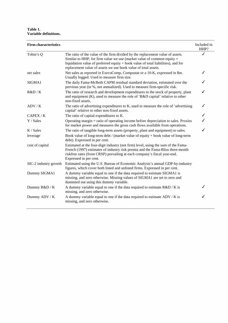
Table 1.Variable definitions.

Firm characteristics Included inHHP?

Tobin’s Q The ratio of the value of the firm divided by the replacement value of assets.Similar to HHP, for firm value we use (market value of common equity +liquidation value of preferred equity + book value of total liabilities), and forreplacement value of assets we use book value of total assets.

�

net sales Net sales as reported in ExecuComp, Compustat or a 10-K, expressed in $m.Usually logged. Used to measure firm size.

�

SIGMA1 The daily Fama-McBeth CAPM residual standard deviation, estimated over theprevious year (in %, not annualized). Used to measure firm-specific risk.

�

R&D / K The ratio of research and development expenditures to the stock of property, plantand equipment (K), used to measure the role of ‘R&D capital’ relative to othernon-fixed assets.

�

ADV / K The ratio of advertising expenditures to K, used to measure the role of ‘advertisingcapital’ relative to other non-fixed assets.

�

CAPEX / K The ratio of capital expenditures to K. �

Y / Sales Operating margin = ratio of operating income before depreciation to sales. Proxiesfor market power and measures the gross cash flows available from operations.

�

K / Sales The ratio of tangible long-term assets (property, plant and equipment) to sales. �

leverage Book value of long-term debt / (market value of equity + book value of long-termdebt). Expressed in per cent.

cost of capital Estimated at the four-digit industry (not firm) level, using the sum of the Fama-French (1997) estimates of industry risk premia and the Fama-Bliss three-monthriskfree rates (from CRSP) prevailing at each company’s fiscal year-end.Expressed in per cent.

SIC-2 industry growth Estimated using the U.S. Bureau of Economic Analysis’s annual GDP-by-industryfigures, which cover both listed and unlisted firms. Expressed in per cent.

Dummy SIGMA1 A dummy variable equal to one if the data required to estimate SIGMA1 ismissing, and zero otherwise. Missing values of SIGMA1 are set to zero anddummied out using this dummy variable.

Dummy R&D / K A dummy variable equal to one if the data required to estimate R&D / K ismissing, and zero otherwise.

�

Dummy ADV / K A dummy variable equal to one if the data required to estimate ADV / K ismissing, and zero otherwise.

�

Table 1. Cont’d.Variable definitions.

Incentive variables Included inHHP?

CEO stockholdings CEO’s common stockholdings as a fraction of common stock outstanding, in percent. Includes beneficial ownership and restricted stock.

�

CEO optionholdings CEO’s optionholdings as a fraction of common stock outstanding, in per cent.total delta The partial derivative of Black-Scholes call option value, adjusted for dividends,

with respect to the price of the underlying stock.vega of options The partial derivative of Black-Scholes call option value, adjusted for dividends,

with respect to the volatility of the underlying stock. Volatility is measured as theannualized standard deviation of daily stock price returns, estimated over the 250trading days preceding the fiscal year in question. In the regressions, we use vegatimes the dollar value of CEO wealth held in options.

capital market pressure = unconditional Pr(delisting), the probability of delisting in each firm’s SIC-2industry in a given panel-year. For each SIC-2 industry and for each panel year,we compute the fraction of all CRSP-listed companies that are delisted due tomerger, bankruptcy, violation of exchange requirements etc, capturing allinvoluntary and voluntary delistings. This measure is unconditional in the sensethat we do not condition the probability of delisting on firm characteristics such assize or prior performance. Expressed in per cent.

product marketpressure

= SIC-4 Herfindahl index, computed as the sum of squared market shares (in %)of each company in an industry, here SIC-4, in a given year. Computed using netsales-market shares for the universe of Compustat firms in 1992-1997.

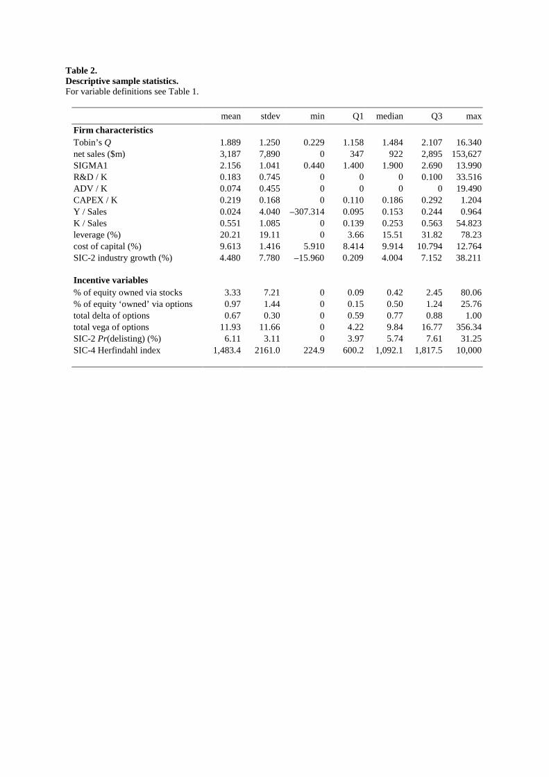
Table 2.Descriptive sample statistics.For variable definitions see Table 1.

mean stdev min Q1 median Q3 max

Firm characteristicsTobin’s Q 1.889 1.250 0.229 1.158 1.484 2.107 16.340net sales ($m) 3,187 7,890 0 347 922 2,895 153,627SIGMA1 2.156 1.041 0.440 1.400 1.900 2.690 13.990R&D / K 0.183 0.745 0 0 0 0.100 33.516ADV / K 0.074 0.455 0 0 0 0 19.490CAPEX / K 0.219 0.168 0 0.110 0.186 0.292 1.204Y / Sales 0.024 4.040 –307.314 0.095 0.153 0.244 0.964K / Sales 0.551 1.085 0 0.139 0.253 0.563 54.823leverage (%) 20.21 19.11 0 3.66 15.51 31.82 78.23cost of capital (%) 9.613 1.416 5.910 8.414 9.914 10.794 12.764SIC-2 industry growth (%) 4.480 7.780 –15.960 0.209 4.004 7.152 38.211

Incentive variables% of equity owned via stocks 3.33 7.21 0 0.09 0.42 2.45 80.06% of equity ‘owned’ via options 0.97 1.44 0 0.15 0.50 1.24 25.76total delta of options 0.67 0.30 0 0.59 0.77 0.88 1.00total vega of options 11.93 11.66 0 4.22 9.84 16.77 356.34SIC-2 Pr(delisting) (%) 6.11 3.11 0 3.97 5.74 7.61 31.25SIC-4 Herfindahl index 1,483.4 2161.0 224.9 600.2 1,092.1 1,817.5 10,000

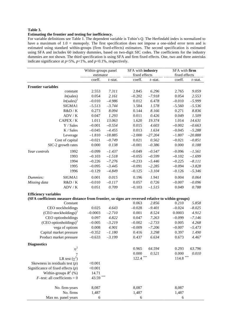
Table 3.Estimating the frontier and testing for inefficiency.For variable definitions see Table 1. The dependent variable is Tobin’s Q. The Herfindahl index is normalized tohave a maximum of 1.0 = monopoly. The first specification does not impose a one-sided error term and isestimated using standard within-groups (firm fixed-effects) estimators. The second specification is estimatedusing SFA and includes 60 industry dummies, based on two-digit SIC codes. The coefficients for the industrydummies are not shown. The third specification is using SFA and firm fixed effects. One, two and three asterisksindicate significance at p<5%, p<1%, and p<0.1%, respectively.

Within-groups panelestimator

SFA with industryfixed effects

SFA with firmfixed effects

coeff. t–stat. coeff. t–stat. coeff. t–stat.

Frontier variablesconstant 2.553 7.311 2.845 6.296 2.765 9.059ln(sales) 0.054 2.161 –0.202 –7.918 0.054 2.553

ln(sales)2 –0.010 –4.986 0.012 6.478 –0.010 –5.999SIGMA1 –5.513 –3.744 1.584 1.578 –5.560 –5.536R&D / K 0.273 8.094 0.144 8.166 0.271 8.836ADV / K 0.047 1.293 0.011 0.426 0.049 1.509

CAPEX / K 1.011 13.063 1.620 19.374 1.014 14.631Y / Sales –0.001 –0.554 0.015 4.603 –0.002 –0.663K / Sales –0.045 –4.455 0.013 1.634 –0.045 –5.288Leverage –1.810 –18.885 –2.000 –27.204 –1.807 –20.888

Cost of capital –0.021 –0.749 0.021 0.562 –0.021 –0.851SIC-2 growth rates 0.000 0.138 –0.001 –0.386 0.000 0.188

Year controls 1992 –0.099 –1.437 –0.049 –0.547 –0.096 –1.5611993 –0.103 –1.518 –0.055 –0.599 –0.102 –1.6991994 –0.226 –7.276 –0.233 –5.446 –0.225 –8.1111995 –0.095 –3.445 –0.091 –2.285 –0.094 –3.8281996 –0.129 –4.849 –0.125 –3.104 –0.126 –5.346

Dummies: SIGMA1 0.001 0.015 0.196 1.941 0.004 0.064Missing data R&D / K –0.010 –0.117 0.057 0.726 –0.007 –0.096

ADV / K 0.051 0.709 –0.103 –1.515 0.049 0.788

Efficiency variables(SFA coefficients measure distance from frontier, so signs are reversed relative to within-groups)

Constant 0.063 2.856 0.210 5.858CEO stockholdings 0.025 4.643 –0.028 –9.401 –0.024 –8.025

(CEO stockholdings)2 –0.0003 –2.710 0.001 8.524 0.0003 4.912CEO optionholdings 0.097 4.822 0.047 7.263 –0.099 –7.146

(CEO optionholdings)2 –0.005 –3.219 –0.002 –2.733 0.005 4.268vega of options 0.008 4.901 –0.009 –7.206 –0.007 –5.473

Capital market pressure –0.352 –1.180 0.416 3.298 0.397 1.490Product market pressure –0.633–3.199 0.437 6.634 0.673 4.467

Diagnostics�

2 0.965 64.594 0.293 63.796� 0.000 0.521 0.000 0.010

LR test (�2) 122.4*** 114.8***

Skewness in residuals test (p) <0.001Significance of fixed effects (p) <0.001

Within-groups R2 (%) 14.71F–test: all coefficients = 0 43.59***

No. firm-years 8,087 8,087 8,087No. firms 1,487 1,487 1,487

Max no. panel years 6 6 6

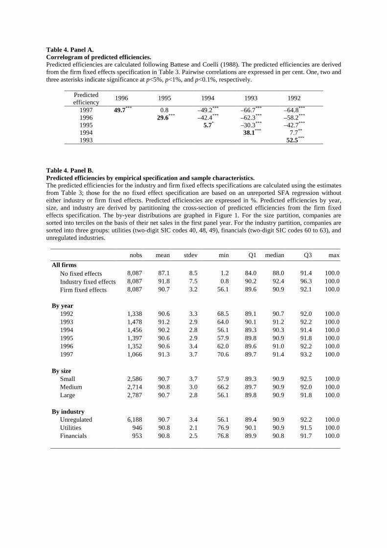
Table 4. Panel A.Correlogram of predicted efficiencies.Predicted efficiencies are calculated following Battese and Coelli (1988). The predicted efficiencies are derivedfrom the firm fixed effects specification in Table 3. Pairwise correlations are expressed in per cent. One, two andthree asterisks indicate significance at p<5%, p<1%, and p<0.1%, respectively.

Predictedefficiency

1996 1995 1994 1993 1992

1997 49.7*** 0.8 –49.2*** –66.7*** –64.8***

1996 29.6*** –42.4*** –62.3*** –58.2***

1995 5.7* –30.3*** –42.7***

1994 38.1*** 7.7**

1993 52.5***

Table 4. Panel B.Predicted efficiencies by empirical specification and sample characteristics.The predicted efficiencies for the industry and firm fixed effects specifications are calculated using the estimatesfrom Table 3; those for the no fixed effect specification are based on an unreported SFA regression withouteither industry or firm fixed effects. Predicted efficiencies are expressed in %. Predicted efficiencies by year,size, and industry are derived by partitioning the cross-section of predicted efficiencies from the firm fixedeffects specification. The by-year distributions are graphed in Figure 1. For the size partition, companies aresorted into terciles on the basis of their net sales in the first panel year. For the industry partition, companies aresorted into three groups: utilities (two-digit SIC codes 40, 48, 49), financials (two-digit SIC codes 60 to 63), andunregulated industries.

nobs mean stdev min Q1 median Q3 max

All firmsNo fixed effects 8,087 87.1 8.5 1.2 84.0 88.0 91.4 100.0Industry fixed effects 8,087 91.8 7.5 0.8 90.2 92.4 96.3 100.0Firm fixed effects 8,087 90.7 3.2 56.1 89.6 90.9 92.1 100.0

By year1992 1,338 90.6 3.3 68.5 89.1 90.7 92.0 100.01993 1,478 91.2 2.9 64.0 90.1 91.2 92.2 100.01994 1,456 90.2 2.8 56.1 89.3 90.3 91.4 100.01995 1,397 90.6 2.9 57.9 89.8 90.9 91.8 100.01996 1,352 90.6 3.4 62.0 89.6 91.0 92.2 100.01997 1,066 91.3 3.7 70.6 89.7 91.4 93.2 100.0

By sizeSmall 2,586 90.7 3.7 57.9 89.3 90.9 92.5 100.0Medium 2,714 90.8 3.0 66.2 89.7 90.9 92.0 100.0Large 2,787 90.7 2.8 56.1 89.8 90.9 91.8 100.0

By industryUnregulated 6,188 90.7 3.4 56.1 89.4 90.9 92.2 100.0Utilities 946 90.8 2.1 76.9 90.1 90.9 91.5 100.0Financials 953 90.8 2.5 76.8 89.9 90.8 91.7 100.0

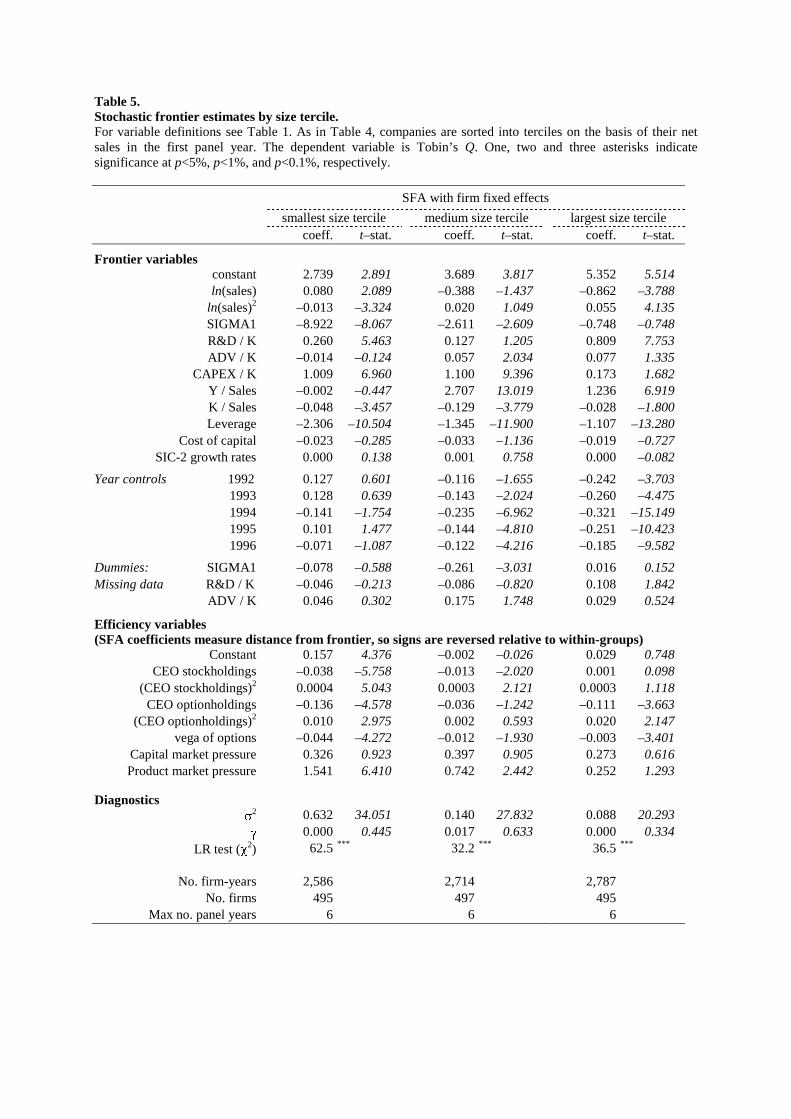
Table 5.Stochastic frontier estimates by size tercile.For variable definitions see Table 1. As in Table 4, companies are sorted into terciles on the basis of their netsales in the first panel year. The dependent variable is Tobin’s Q. One, two and three asterisks indicatesignificance at p<5%, p<1%, and p<0.1%, respectively.

SFA with firm fixed effects

smallest size tercile medium size tercile largest size tercilecoeff. t–stat. coeff. t–stat. coeff. t–stat.

Frontier variablesconstant 2.739 2.891 3.689 3.817 5.352 5.514ln(sales) 0.080 2.089 –0.388 –1.437 –0.862 –3.788

ln(sales)2 –0.013 –3.324 0.020 1.049 0.055 4.135SIGMA1 –8.922 –8.067 –2.611 –2.609 –0.748 –0.748R&D / K 0.260 5.463 0.127 1.205 0.809 7.753ADV / K –0.014 –0.124 0.057 2.034 0.077 1.335

CAPEX / K 1.009 6.960 1.100 9.396 0.173 1.682Y / Sales –0.002 –0.447 2.707 13.019 1.236 6.919K / Sales –0.048 –3.457 –0.129 –3.779 –0.028 –1.800Leverage –2.306 –10.504 –1.345 –11.900 –1.107 –13.280

Cost of capital –0.023 –0.285 –0.033 –1.136 –0.019 –0.727SIC-2 growth rates 0.000 0.138 0.001 0.758 0.000 –0.082

Year controls 1992 0.127 0.601 –0.116 –1.655 –0.242 –3.7031993 0.128 0.639 –0.143 –2.024 –0.260 –4.4751994 –0.141 –1.754 –0.235 –6.962 –0.321 –15.1491995 0.101 1.477 –0.144 –4.810 –0.251 –10.4231996 –0.071 –1.087 –0.122 –4.216 –0.185 –9.582

Dummies: SIGMA1 –0.078 –0.588 –0.261 –3.031 0.016 0.152Missing data R&D / K –0.046 –0.213 –0.086 –0.820 0.108 1.842

ADV / K 0.046 0.302 0.175 1.748 0.029 0.524

Efficiency variables(SFA coefficients measure distance from frontier, so signs are reversed relative to within-groups)

Constant 0.157 4.376 –0.002 –0.026 0.029 0.748CEO stockholdings –0.038 –5.758 –0.013 –2.020 0.001 0.098

(CEO stockholdings)2 0.0004 5.043 0.0003 2.121 0.0003 1.118CEO optionholdings –0.136 –4.578 –0.036 –1.242 –0.111 –3.663

(CEO optionholdings)2 0.010 2.975 0.002 0.593 0.020 2.147vega of options –0.044 –4.272 –0.012 –1.930 –0.003 –3.401

Capital market pressure 0.326 0.923 0.397 0.905 0.273 0.616Product market pressure 1.541 6.410 0.742 2.442 0.252 1.293

Diagnostics�

2 0.632 34.051 0.140 27.832 0.088 20.293� 0.000 0.445 0.017 0.633 0.000 0.334

LR test (�2) 62.5 *** 32.2 *** 36.5 ***

No. firm-years 2,586 2,714 2,787No. firms 495 497 495

Max no. panel years 6 6 6

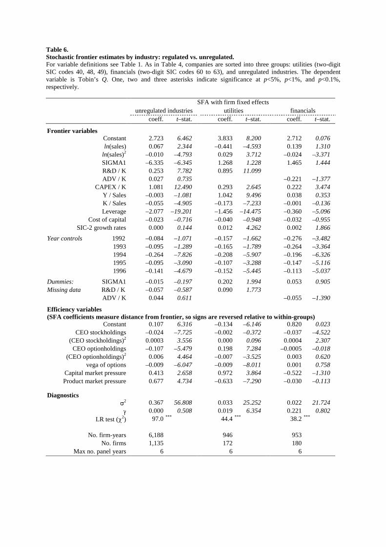
Table 6.Stochastic frontier estimates by industry: regulated vs. unregulated.For variable definitions see Table 1. As in Table 4, companies are sorted into three groups: utilities (two-digitSIC codes 40, 48, 49), financials (two-digit SIC codes 60 to 63), and unregulated industries. The dependentvariable is Tobin’s Q. One, two and three asterisks indicate significance at p<5%, p<1%, and p<0.1%,respectively.

SFA with firm fixed effectsunregulated industries utilities financials

coeff. t–stat. coeff. t–stat. coeff. t–stat.

Frontier variablesConstant 2.723 6.462 3.833 8.200 2.712 0.076ln(sales) 0.067 2.344 –0.441 –4.593 0.139 1.310

ln(sales)2 –0.010 –4.793 0.029 3.712 –0.024 –3.371SIGMA1 –6.335 –6.345 1.268 1.228 1.465 1.444R&D / K 0.253 7.782 0.895 11.099ADV / K 0.027 0.735 –0.221 –1.377

CAPEX / K 1.081 12.490 0.293 2.645 0.222 3.474Y / Sales –0.003 –1.081 1.042 9.496 0.038 0.353K / Sales –0.055 –4.905 –0.173 –7.233 –0.001 –0.136Leverage –2.077 –19.201 –1.456 –14.475 –0.360 –5.096

Cost of capital –0.023 –0.716 –0.040 –0.948 –0.032 –0.955SIC-2 growth rates 0.000 0.144 0.012 4.262 0.002 1.866

Year controls 1992 –0.084 –1.071 –0.157 –1.662 –0.276 –3.4821993 –0.095 –1.289 –0.165 –1.789 –0.264 –3.3641994 –0.264 –7.826 –0.208 –5.907 –0.196 –6.3261995 –0.095 –3.090 –0.107 –3.288 –0.147 –5.1161996 –0.141 –4.679 –0.152 –5.445 –0.113 –5.037

Dummies: SIGMA1 –0.015 –0.197 0.202 1.994 0.053 0.905Missing data R&D / K –0.057 –0.587 0.090 1.773

ADV / K 0.044 0.611 –0.055 –1.390

Efficiency variables(SFA coefficients measure distance from frontier, so signs are reversed relative to within-groups)

Constant 0.107 6.316 –0.134 –6.146 0.820 0.023CEO stockholdings –0.024 –7.725 –0.002 –0.372 –0.037 –4.522

(CEO stockholdings)2 0.0003 3.556 0.000 0.096 0.0004 2.307CEO optionholdings –0.107 –5.479 0.198 7.284 –0.0005 –0.018

(CEO optionholdings)2 0.006 4.464 –0.007 –3.525 0.003 0.620vega of options –0.009 –6.047 –0.009 –8.011 0.001 0.758

Capital market pressure 0.413 2.658 0.972 3.864 –0.522 –1.310Product market pressure 0.677 4.734 –0.633 –7.290 –0.030 –0.113

Diagnostics�

2 0.367 56.808 0.033 25.252 0.022 21.724� 0.000 0.508 0.019 6.354 0.221 0.802

LR test (�2) 97.0 *** 44.4 *** 38.2 ***

No. firm-years 6,188 946 953No. firms 1,135 172 180

Max no. panel years 6 6 6

Table 7.Board reactions to managerial inefficiency.Predicted efficiencies are calculated following Battese and Coelli (1988) using the SFA firm fixed effectsestimates from Table 3. They are lagged one year, resulting in a smaller 5-year panel with 6,600 firm-years. Thevalue of restricted stock awards and of option awards are in $’000s. ExecuComp values option awards using amodified form of Black-Scholes. Cash salary is base salary plus all other monetary compensation, but excludesbonus and long-term incentive payments. Bonus is annual bonus payments and excludes long-term incentivepayments. Cash salary and bonus are in $’000s. The logit model of CEO replacement uses a dummy equal to oneif a CEO aged 60 or under is replaced in year t, and zero else. The dummy does not distinguish between forcedand voluntary CEO replacement, though the age condition is intended to control for retirements. For othervariable definitions see Table 1. Within-groups are fixed-effects panel data regressions. Logits are estimatedwith fixed effects (a.k.a. conditional). Tobits are estimated with random effects (given that fixed effects Tobitsare inconsistent) with censoring at 0. Standard errors are given in italics below the coefficient estimates. One,two and three asterisks indicate significance at p<5%, p<1%, and p<0.1%, respectively.

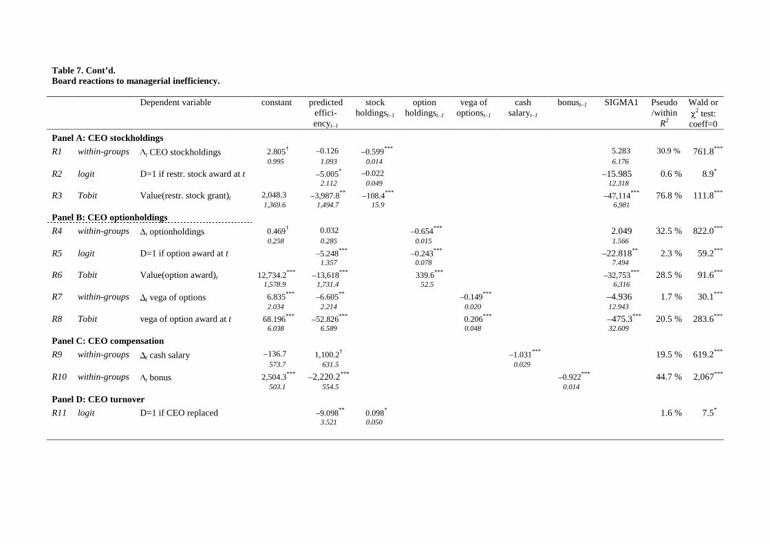
Table 7. Cont’d.Board reactions to managerial inefficiency.

Dependent variable constant predictedeffici-encyt–1

stockholdingst–1

optionholdingst–1

vega ofoptionst–1

cashsalaryt–1

bonust–1 SIGMA1 Pseudo/within

R2

Wald or�

2 test:coeff=0

Panel A: CEO stockholdings

R1 within-groups �t CEO stockholdings 2.805† –0.126 –0.599*** 5.283 30.9 % 761.8***

0.995 1.093 0.014 6.176

R2 logit D=1 if restr. stock award at t –5.005* –0.022 –15.985 0.6 % 8.9*

2.112 0.049 12.318

R3 Tobit Value(restr. stock grant)t 2,048.3 –3,987.8** –108.4*** –47,114*** 76.8 % 111.8***

1,369.6 1,494.7 15.9 6,981

Panel B: CEO optionholdings

R4 within-groups �t optionholdings 0.469† 0.032 –0.654*** 2.049 32.5 % 822.0***

0.258 0.285 0.015 1.566

R5 logit D=1 if option award at t –5.248*** –0.243*** –22.818** 2.3 % 59.2***

1.357 0.078 7.494

R6 Tobit Value(option award)t 12,734.2*** –13,618*** 339.6*** –32,753*** 28.5 % 91.6***

1,578.9 1,731.4 52.5 6,316

R7 within-groups �t vega of options 6.835*** –6.605** –0.149*** –4.936 1.7 % 30.1***

2.034 2.214 0.020 12.943

R8 Tobit vega of option award at t 68.196*** –52.826*** 0.206*** –475.3*** 20.5 % 283.6***

6.038 6.589 0.048 32.609

Panel C: CEO compensation

R9 within-groups �t cash salary –136.7 1,100.2† –1.031*** 19.5 % 619.2***

573.7 631.5 0.029

R10 within-groups �t bonus 2,504.3*** –2,220.2*** –0.922*** 44.7 % 2,067***

503.1 554.5 0.014

Panel D: CEO turnover

R11 logit D=1 if CEO replaced –9.098** 0.098* 1.6 % 7.5*

3.521 0.050

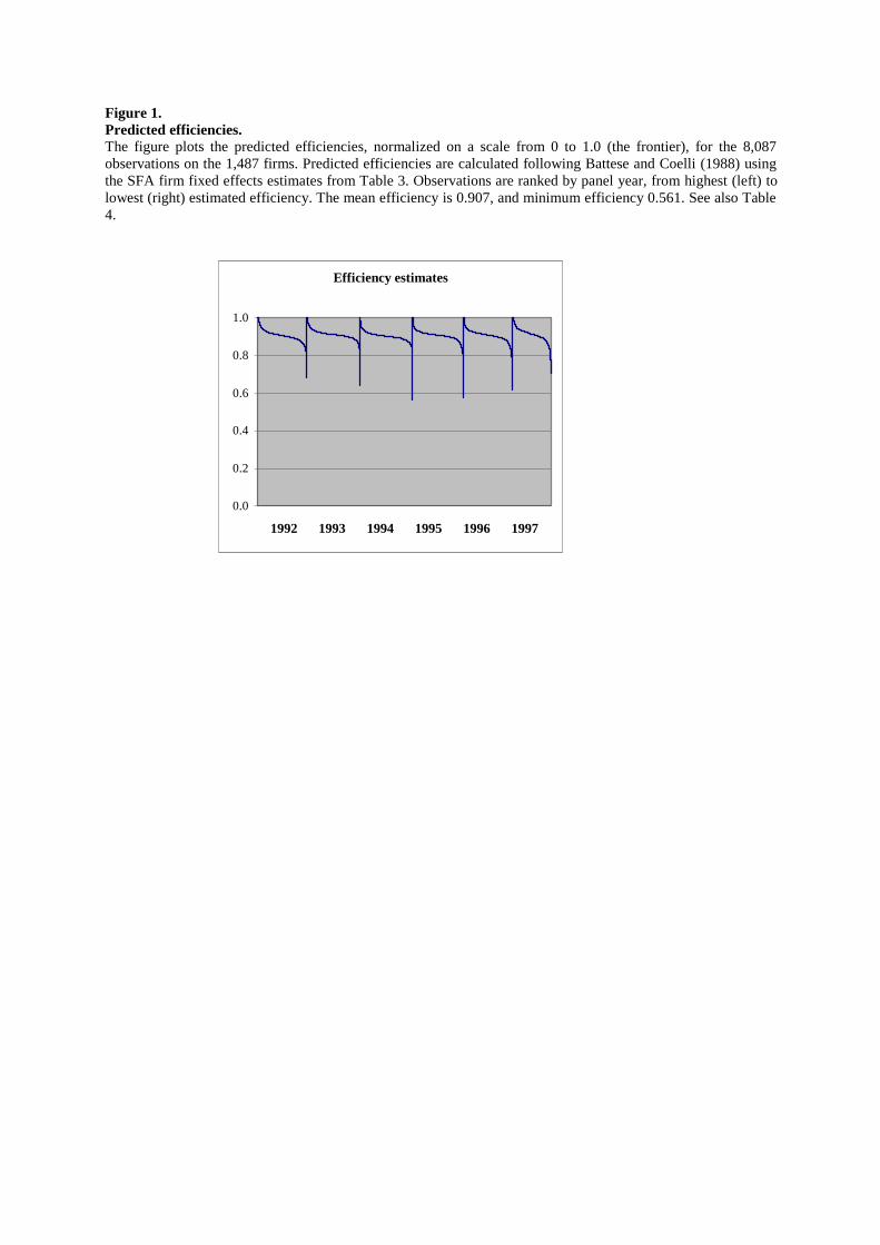
Figure 1.Predicted efficiencies.The figure plots the predicted efficiencies, normalized on a scale from 0 to 1.0 (the frontier), for the 8,087observations on the 1,487 firms. Predicted efficiencies are calculated following Battese and Coelli (1988) usingthe SFA firm fixed effects estimates from Table 3. Observations are ranked by panel year, from highest (left) tolowest (right) estimated efficiency. The mean efficiency is 0.907, and minimum efficiency 0.561. See also Table4.

Efficiency estimates

0.0

0.2

0.4

0.6

0.8

1.0

1992 1993 1994 1995 1996 1997