Embed Size (px)
Citation preview
Aims The Economy Stationary Equilibrium Technical Progress Summary
Firm Dynamics in the Neoclassical Growth Model
Omar LicandroUniversity of Nottingham
2015 RIDGE December Forum
1 / 26

Aims The Economy Stationary Equilibrium Technical Progress Summary
Ramsey-Hopenhayn Model
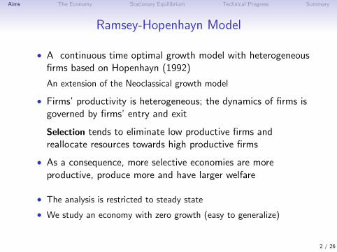
• A continuous time optimal growth model with heterogeneousfirms based on Hopenhayn (1992)
An extension of the Neoclassical growth model
• Firms’ productivity is heterogeneous; the dynamics of firms isgoverned by firms’ entry and exit
Selection tends to eliminate low productive firms andreallocate resources towards high productive firms
• As a consequence, more selective economies are moreproductive, produce more and have larger welfare
• The analysis is restricted to steady state
• We study an economy with zero growth (easy to generalize)
2 / 26
Aims The Economy Stationary Equilibrium Technical Progress Summary
Ramsey-Hopenhayn Model
• A continuous time optimal growth model with heterogeneousfirms based on Hopenhayn (1992)
An extension of the Neoclassical growth model
• Firms’ productivity is heterogeneous; the dynamics of firms isgoverned by firms’ entry and exit
Selection tends to eliminate low productive firms andreallocate resources towards high productive firms
• As a consequence, more selective economies are moreproductive, produce more and have larger welfare
• The analysis is restricted to steady state
• We study an economy with zero growth (easy to generalize)
2 / 26
Aims The Economy Stationary Equilibrium Technical Progress Summary
The model
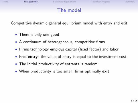
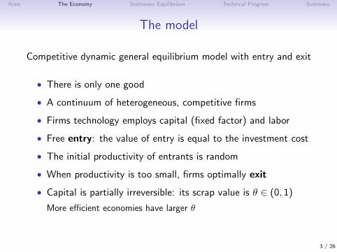
Competitive dynamic general equilibrium model with entry and exit
• There is only one good
• A continuum of heterogeneous, competitive firms
• Firms technology employs capital (fixed factor) and labor
• Free entry: the value of entry is equal to the investment cost
• The initial productivity of entrants is random
• When productivity is too small, firms optimally exit
• Capital is partially irreversible: its scrap value is θ ∈ (0, 1)
More efficient economies have larger θ
3 / 26
Aims The Economy Stationary Equilibrium Technical Progress Summary
The model
Competitive dynamic general equilibrium model with entry and exit
• There is only one good
• A continuum of heterogeneous, competitive firms
• Firms technology employs capital (fixed factor) and labor
• Free entry: the value of entry is equal to the investment cost
• The initial productivity of entrants is random
• When productivity is too small, firms optimally exit
• Capital is partially irreversible: its scrap value is θ ∈ (0, 1)
More efficient economies have larger θ
3 / 26
Aims The Economy Stationary Equilibrium Technical Progress Summary
Preferences
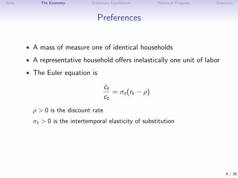
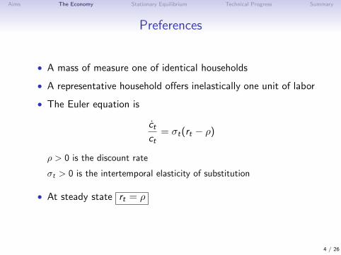
• A mass of measure one of identical households
• A representative household offers inelastically one unit of labor
• The Euler equation is
ctct
= σt(rt − ρ)
ρ > 0 is the discount rate
σt > 0 is the intertemporal elasticity of substitution
• At steady state rt = ρ
4 / 26
Aims The Economy Stationary Equilibrium Technical Progress Summary
Preferences
• A mass of measure one of identical households
• A representative household offers inelastically one unit of labor
• The Euler equation is
ctct
= σt(rt − ρ)
ρ > 0 is the discount rate
σt > 0 is the intertemporal elasticity of substitution
• At steady state rt = ρ
4 / 26

Aims The Economy Stationary Equilibrium Technical Progress Summary
Technology
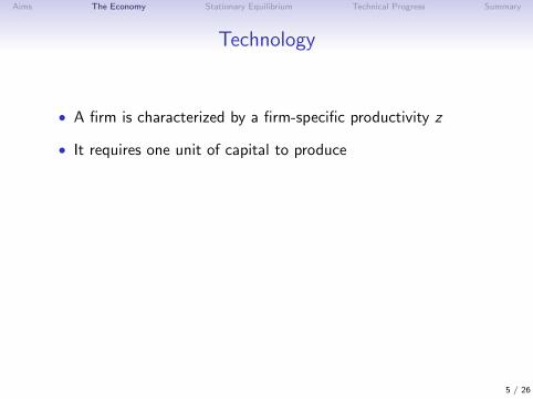
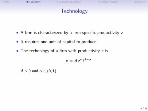
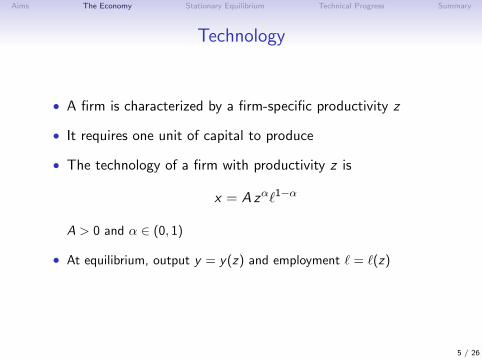
• A firm is characterized by a firm-specific productivity z
• It requires one unit of capital to produce
• The technology of a firm with productivity z is
x = A zα`1−α
A > 0 and α ∈ (0, 1)
• At equilibrium, output y = y(z) and employment ` = `(z)
5 / 26

Aims The Economy Stationary Equilibrium Technical Progress Summary
Technology
• A firm is characterized by a firm-specific productivity z
• It requires one unit of capital to produce
• The technology of a firm with productivity z is
x = A zα`1−α
A > 0 and α ∈ (0, 1)
• At equilibrium, output y = y(z) and employment ` = `(z)
5 / 26

Aims The Economy Stationary Equilibrium Technical Progress Summary
Entry and Exit
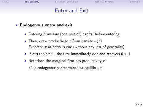
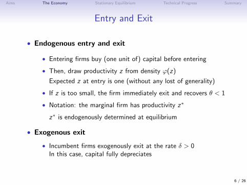
• Endogenous entry and exit
• Entering firms buy (one unit of) capital before entering
• Then, draw productivity z from density ϕ(z)
Expected z at entry is one (without any lost of generality)
• If z is too small, the firm immediately exit and recovers θ < 1
• Notation: the marginal firm has productivity z∗
z∗ is endogenously determined at equilibrium
• Exogenous exit
• Incumbent firms exogenously exit at the rate δ > 0In this case, capital fully depreciates
6 / 26

Aims The Economy Stationary Equilibrium Technical Progress Summary
Entry and Exit
• Endogenous entry and exit
• Entering firms buy (one unit of) capital before entering
• Then, draw productivity z from density ϕ(z)
Expected z at entry is one (without any lost of generality)
• If z is too small, the firm immediately exit and recovers θ < 1
• Notation: the marginal firm has productivity z∗
z∗ is endogenously determined at equilibrium
• Exogenous exit
• Incumbent firms exogenously exit at the rate δ > 0In this case, capital fully depreciates
6 / 26
Aims The Economy Stationary Equilibrium Technical Progress Summary
Equilibrium Distribution
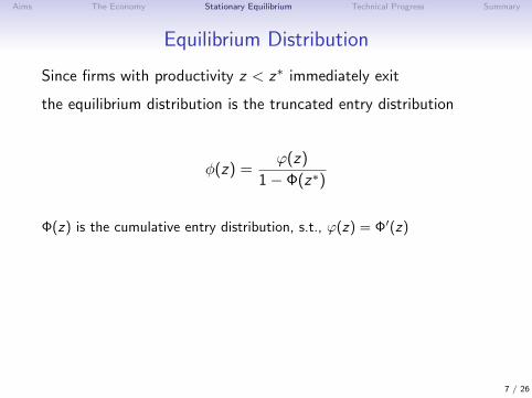
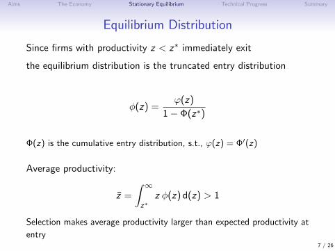
Since firms with productivity z < z∗ immediately exit
the equilibrium distribution is the truncated entry distribution
φ(z) =ϕ(z)
1− Φ(z∗)
Φ(z) is the cumulative entry distribution, s.t., ϕ(z) = Φ′(z)
Average productivity:
z =
∫ ∞z∗
z φ(z) d(z) > 1
Selection makes average productivity larger than expected productivity at
entry
7 / 26
Aims The Economy Stationary Equilibrium Technical Progress Summary
Equilibrium Distribution
Since firms with productivity z < z∗ immediately exit
the equilibrium distribution is the truncated entry distribution
φ(z) =ϕ(z)
1− Φ(z∗)
Φ(z) is the cumulative entry distribution, s.t., ϕ(z) = Φ′(z)
Average productivity:
z =
∫ ∞z∗
z φ(z) d(z) > 1
Selection makes average productivity larger than expected productivity at
entry7 / 26
Aims The Economy Stationary Equilibrium Technical Progress Summary
Firms’ Problem
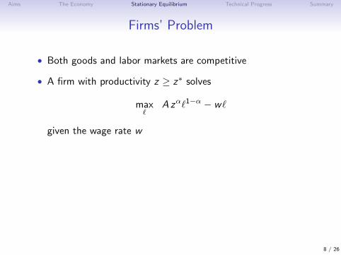
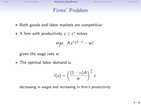
• Both goods and labor markets are competitive
• A firm with productivity z ≥ z∗ solves
max`
A zα`1−α − w`
given the wage rate w
• The optimal labor demand is
`(z) =
((1− α)A
w
) 1α
z
decreasing in wages and increasing in firm’s productivity
8 / 26

Aims The Economy Stationary Equilibrium Technical Progress Summary
Firms’ Problem
• Both goods and labor markets are competitive
• A firm with productivity z ≥ z∗ solves
max`
A zα`1−α − w`
given the wage rate w
• The optimal labor demand is
`(z) =
((1− α)A
w
) 1α
z
decreasing in wages and increasing in firm’s productivity
8 / 26

Aims The Economy Stationary Equilibrium Technical Progress Summary
Labor market equilibrium
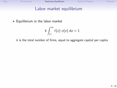
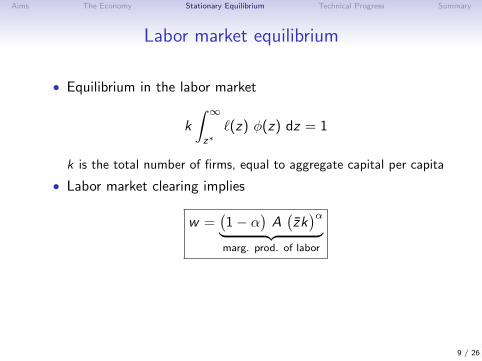
• Equilibrium in the labor market
k
∫ ∞z∗
`(z) φ(z) dz = 1
k is the total number of firms, equal to aggregate capital per capita
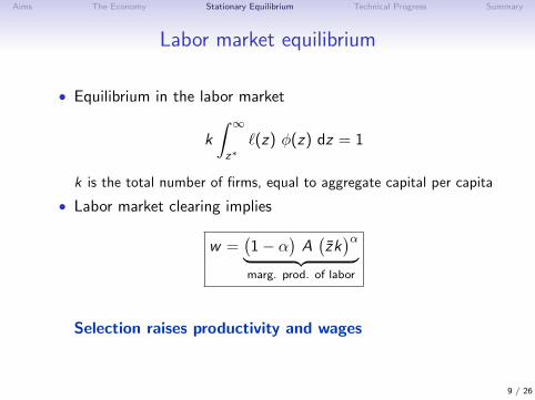
• Labor market clearing implies
w =(1− α
)A(zk)α︸ ︷︷ ︸
marg. prod. of labor
Selection raises productivity and wages
9 / 26
Aims The Economy Stationary Equilibrium Technical Progress Summary
Labor market equilibrium
• Equilibrium in the labor market
k
∫ ∞z∗
`(z) φ(z) dz = 1
k is the total number of firms, equal to aggregate capital per capita
• Labor market clearing implies
w =(1− α
)A(zk)α︸ ︷︷ ︸
marg. prod. of labor
Selection raises productivity and wages
9 / 26
Aims The Economy Stationary Equilibrium Technical Progress Summary
Aggregate Output
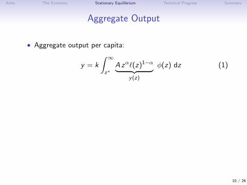
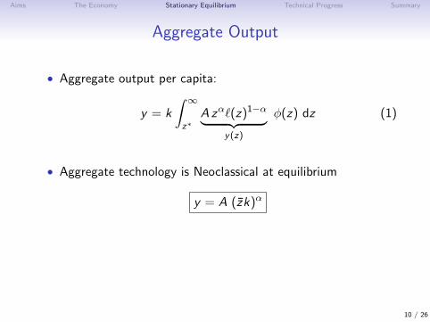
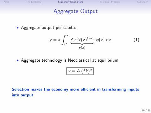
• Aggregate output per capita:
y = k
∫ ∞z∗
A zα`(z)1−α︸ ︷︷ ︸y(z)
φ(z) dz (1)
• Aggregate technology is Neoclassical at equilibrium
y = A (zk)α
Selection makes the economy more efficient in transforming inputs
into output
10 / 26
Aims The Economy Stationary Equilibrium Technical Progress Summary
Aggregate Output
• Aggregate output per capita:
y = k
∫ ∞z∗
A zα`(z)1−α︸ ︷︷ ︸y(z)
φ(z) dz (1)
• Aggregate technology is Neoclassical at equilibrium
y = A (zk)α
Selection makes the economy more efficient in transforming inputs
into output
10 / 26
Aims The Economy Stationary Equilibrium Technical Progress Summary
Aggregate Output: General Case
• Assumex = F (z , `)
where F (.) is a Neoclassic production function
• Aggregate output per capita is
y = F (zk, 1) = f (zk)
Aggregate technology is Neoclassic
Capital is measured in efficiency units
11 / 26

Aims The Economy Stationary Equilibrium Technical Progress Summary
Firm’s Value
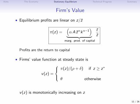
• Equilibrium profits are linear on z/z
π(z) =(αA zαkα−1
)︸ ︷︷ ︸
marg. prod. of capital
z
z
Profits are the return to capital
• Firms’ value function at steady state is
v(z) =
π(z)/(ρ+ δ) if z ≥ z∗
θ otherwise
v(z) is monotonically increasing on z
12 / 26
Aims The Economy Stationary Equilibrium Technical Progress Summary
Firm’s Value
• Equilibrium profits are linear on z/z
π(z) =(αA zαkα−1
)︸ ︷︷ ︸
marg. prod. of capital
z
z
Profits are the return to capital
• Firms’ value function at steady state is
v(z) =
π(z)/(ρ+ δ) if z ≥ z∗
θ otherwise
v(z) is monotonically increasing on z
12 / 26

Aims The Economy Stationary Equilibrium Technical Progress Summary
Equilibrium Exit
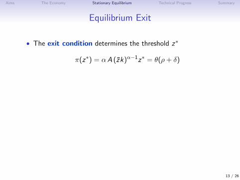
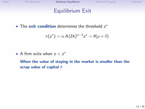
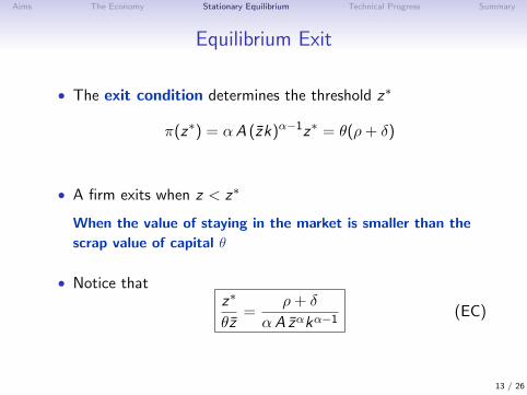
• The exit condition determines the threshold z∗
π(z∗) = αA (zk)α−1z∗ = θ(ρ+ δ)
• A firm exits when z < z∗
When the value of staying in the market is smaller than the
scrap value of capital θ
• Notice thatz∗
θz=
ρ+ δ
αA zαkα−1(EC)
13 / 26
Aims The Economy Stationary Equilibrium Technical Progress Summary
Equilibrium Exit
• The exit condition determines the threshold z∗
π(z∗) = αA (zk)α−1z∗ = θ(ρ+ δ)
• A firm exits when z < z∗
When the value of staying in the market is smaller than the
scrap value of capital θ
• Notice thatz∗
θz=
ρ+ δ
αA zαkα−1(EC)
13 / 26

Aims The Economy Stationary Equilibrium Technical Progress Summary
Equilibrium Entry
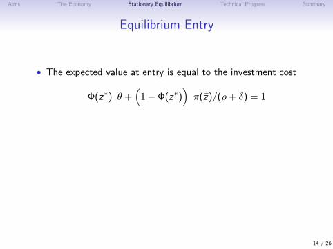
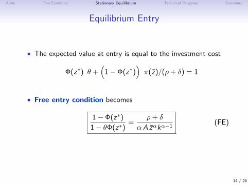
• The expected value at entry is equal to the investment cost
Φ(z∗) θ +(
1− Φ(z∗))π(z)/(ρ+ δ) = 1
• Free entry condition becomes
1− Φ(z∗)
1− θΦ(z∗)=
ρ+ δ
αA zαkα−1(FE)
14 / 26
Aims The Economy Stationary Equilibrium Technical Progress Summary
Equilibrium Entry
• The expected value at entry is equal to the investment cost
Φ(z∗) θ +(
1− Φ(z∗))π(z)/(ρ+ δ) = 1
• Free entry condition becomes
1− Φ(z∗)
1− θΦ(z∗)=
ρ+ δ
αA zαkα−1(FE)
14 / 26
Aims The Economy Stationary Equilibrium Technical Progress Summary
Equilibrium Entry
• The expected value at entry is equal to the investment cost
Φ(z∗) θ +(
1− Φ(z∗))π(z)/(ρ+ δ) = 1
• Free entry condition becomes
1− Φ(z∗)
1− θΦ(z∗)=
ρ+ δ
αA zαkα−1(FE)
14 / 26

Aims The Economy Stationary Equilibrium Technical Progress Summary
Equilibrium Cutoff
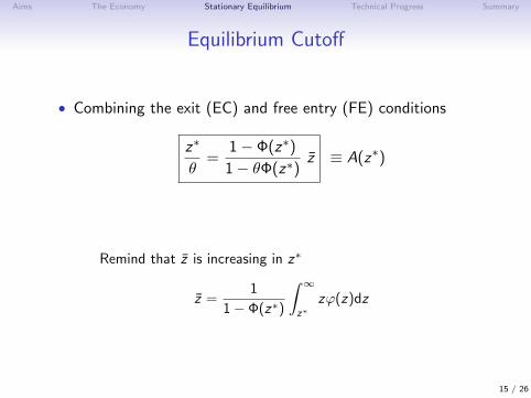
• Combining the exit (EC) and free entry (FE) conditions
z∗
θ=
1− Φ(z∗)
1− θΦ(z∗)z ≡ A(z∗)
Remind that z is increasing in z∗
z =1
1− Φ(z∗)
∫ ∞z∗
zϕ(z)dz
15 / 26
Aims The Economy Stationary Equilibrium Technical Progress Summary
Equilibrium Cutoff
• Combining the exit (EC) and free entry (FE) conditions
z∗
θ=
1− Φ(z∗)
1− θΦ(z∗)z ≡ A(z∗)
Remind that z is increasing in z∗
z =1
1− Φ(z∗)
∫ ∞z∗
zϕ(z)dz
15 / 26
Aims The Economy Stationary Equilibrium Technical Progress Summary
Equilibrium Cutoff
• Proposition 1: z∗ exists and is unique
• Corollary: z∗ ≥ θ
It is always better to close down when productivity is smaller than
the scrap value
16 / 26
Aims The Economy Stationary Equilibrium Technical Progress Summary
Equilibrium Cutoff
• Proposition 1: z∗ exists and is unique
• Corollary: z∗ ≥ θ
It is always better to close down when productivity is smaller than
the scrap value
16 / 26
Aims The Economy Stationary Equilibrium Technical Progress Summary
Equilibrium Cutoff
• Proposition 1: z∗ exists and is unique
• Corollary: z∗ ≥ θ
It is always better to close down when productivity is smaller than
the scrap value
16 / 26
Aims The Economy Stationary Equilibrium Technical Progress Summary
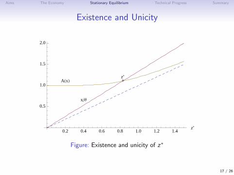
Existence and Unicity
0.2 0.4 0.6 0.8 1.0 1.2 1.4z*
0.5
1.0
1.5
2.0
AHxL
x�Θ
ë
z*
ë
Figure: Existence and unicity of z∗
17 / 26
Aims The Economy Stationary Equilibrium Technical Progress Summary
Selection and Capital Irreversibility
• Proposition 2:dz∗
dθ> 1
• More reversible capital is, more the economy is selective
• Efficiency
• A reduction in the degree of irreversibility (θ)
• Generates productivity gains through selection (z)
18 / 26
Aims The Economy Stationary Equilibrium Technical Progress Summary
Selection and Productivity Dispertion
• Proposition 3:dz∗
dσ> 0 (σ = variance of the entry
distribution)
Larger the variance is, more likely is to get a high productivity
19 / 26
Aims The Economy Stationary Equilibrium Technical Progress Summary
Selection and Productivity Dispertion
• Proposition 3:dz∗
dσ> 0 (σ = variance of the entry
distribution)
Larger the variance is, more likely is to get a high productivity
19 / 26
Aims The Economy Stationary Equilibrium Technical Progress Summary
Neoclassical Model A
• The Neoclassical Model corresponds to the extreme case of adegenerate entry distribution with zero variance
There is a representative firm with productivity z = z = 1
• Per capita output is y = Akα
• Wages w = (1− α)Akα
• Profits are π = αAkα−1
The free entry condition makes ρ+ δ = αAkα−1
• Irreversibility plays no role: (FE) ⇒ v(1) > θ
The representative firm never exits
20 / 26
Aims The Economy Stationary Equilibrium Technical Progress Summary
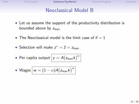
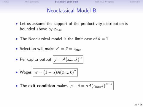
Neoclassical Model B
• Let us assume the support of the productivity distribution isbounded above by zmax
• The Neoclassical model is the limit case of θ = 1
• Selection will make z∗ = z = zmax
• Per capita output y = A(zmaxk
)α• Wages w = (1− α)A
(zmaxk
)α• The exit condition makes ρ+ δ = αA
(zmaxk
)α−1
21 / 26
Aims The Economy Stationary Equilibrium Technical Progress Summary
Neoclassical Model B
• Let us assume the support of the productivity distribution isbounded above by zmax
• The Neoclassical model is the limit case of θ = 1
• Selection will make z∗ = z = zmax
• Per capita output y = A(zmaxk
)α
• Wages w = (1− α)A(zmaxk
)α• The exit condition makes ρ+ δ = αA
(zmaxk
)α−1
21 / 26
Aims The Economy Stationary Equilibrium Technical Progress Summary
Neoclassical Model B
• Let us assume the support of the productivity distribution isbounded above by zmax
• The Neoclassical model is the limit case of θ = 1
• Selection will make z∗ = z = zmax
• Per capita output y = A(zmaxk
)α• Wages w = (1− α)A
(zmaxk
)α
• The exit condition makes ρ+ δ = αA(zmaxk
)α−1
21 / 26
Aims The Economy Stationary Equilibrium Technical Progress Summary
Neoclassical Model B
• Let us assume the support of the productivity distribution isbounded above by zmax
• The Neoclassical model is the limit case of θ = 1
• Selection will make z∗ = z = zmax
• Per capita output y = A(zmaxk
)α• Wages w = (1− α)A
(zmaxk
)α• The exit condition makes ρ+ δ = αA
(zmaxk
)α−1
21 / 26
Aims The Economy Stationary Equilibrium Technical Progress Summary
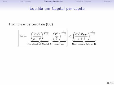
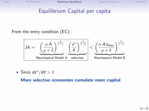
Equilibrium Capital per capita
From the entry condition (EC)
zk =
(αA
ρ+ δ
) 11−α
︸ ︷︷ ︸Neoclassical Model A
(z∗
θ
) 11−α
︸ ︷︷ ︸selection
<
(αA zmax
ρ+ δ
) 11−α
︸ ︷︷ ︸Neoclassical Model B
• Since dz∗/dθ > 1
More selective economies cumulate more capital
22 / 26
Aims The Economy Stationary Equilibrium Technical Progress Summary
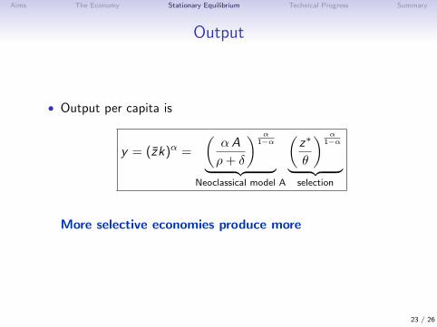
Output
• Output per capita is
y = (zk)α =
(αA
ρ+ δ
) α1−α
︸ ︷︷ ︸Neoclassical model A
(z∗
θ
) α1−α
︸ ︷︷ ︸selection
More selective economies produce more
23 / 26
Aims The Economy Stationary Equilibrium Technical Progress Summary
Output
• Output per capita is
y = (zk)α =
(αA
ρ+ δ
) α1−α
︸ ︷︷ ︸Neoclassical model A
(z∗
θ
) α1−α
︸ ︷︷ ︸selection
More selective economies produce more
23 / 26

Aims The Economy Stationary Equilibrium Technical Progress Summary
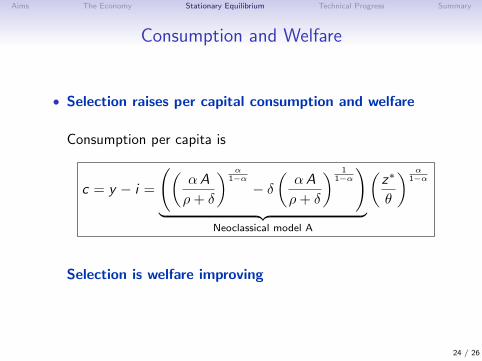
Consumption and Welfare
• Selection raises per capital consumption and welfare
Consumption per capita is
c = y − i =
((αA
ρ+ δ
) α1−α
− δ(αA
ρ+ δ
) 11−α
)︸ ︷︷ ︸
Neoclassical model A
(z∗
θ
) α1−α
Selection is welfare improving
24 / 26
Aims The Economy Stationary Equilibrium Technical Progress Summary
Technical Progress
The model can be extended to the case of exogenous growth
Assume the productivity of incumbent firms grow at the exogenous rate
γ > 0 and the entry distribution Φt(z) has expected productivity at entry
equal to eγt
25 / 26
Aims The Economy Stationary Equilibrium Technical Progress Summary
Summary
• The Ramsey-Hopenhayn model has the Neoclassical model asa limit case
• Idiosyncratic uncertainty increases the probability of highproductivity events to occur, raising selection
• Capital reversibility is good, raising selection too
• More selective economies are more productivity, produce moreoutput and welfare
• More selective economies reallocate labor from less to moreproductive firms through a higher wage rate
26 / 26