Embed Size (px)
Citation preview

Firm Dynamics and Residual Inequality in Open Economies
Gabriel Felbermayr Giammario Impullitti
Julien Prat
CESIFO WORKING PAPER NO. 4666 CATEGORY 8: TRADE POLICY
ORIGINAL VERSION: FEBRUARY 2014 THIS VERSION: JUNE 2016
An electronic version of the paper may be downloaded • from the SSRN website: www.SSRN.com • from the RePEc website: www.RePEc.org
• from the CESifo website: Twww.CESifo-group.org/wp T
CESifo Working Paper No. 4666
Firm Dynamics and Residual Inequality in Open Economies
Abstract
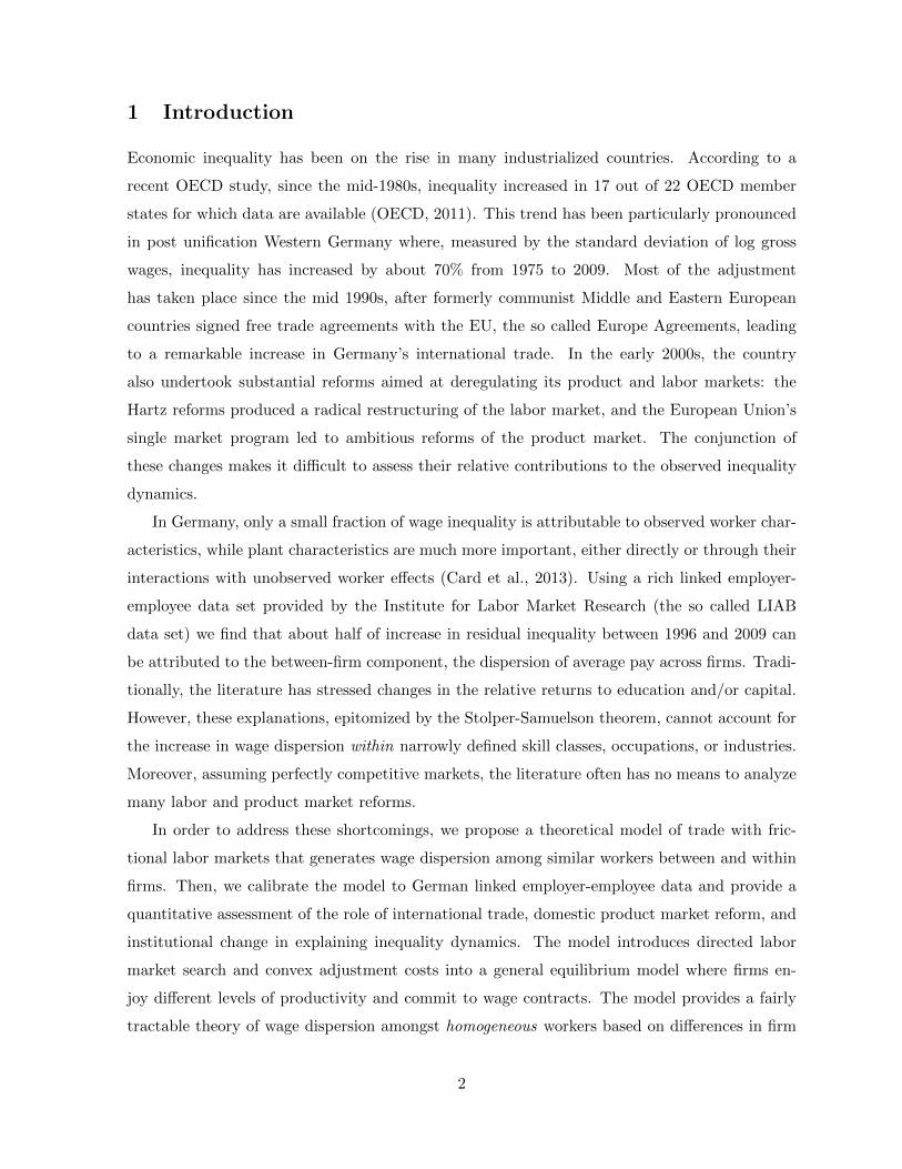
Wage inequality between similar workers has been on the rise in many rich countries. Recent empirical research suggests that heterogeneity in firm characteristics is crucial to understand wage dispersion. Lower trade costs as well as labor and product market reforms are considered critical drivers of inequality dynamics. We ask how these factors affect wage dispersion and how much of their effect on inequality is attributable to changes in wage dispersion between and within firms. To tackle these questions, we incorporate directed job search into a dynamic model of international trade where wage inequality results from the interplay of convex adjustment costs with firms’ different hiring needs along their life cycles. Fitting the model to German linked employer-employee data for the years 1996-2009, we find that firm heterogeneity explains about half of the surge in inequality. The most important mechanism is tougher product market competition driven by domestic product market deregulation and, indirectly, by international trade.
JEL-Code: F120, F160, E240.
Keywords: wage inequality, international trade, directed search, firm dynamics, product and labor market regulation.
Gabriel Felbermayr
Ifo Institute – Leibniz Institute for Economic Research at the University of Munich
Munich / Germany [email protected]
Giammario Impullitti University of Nottingham / UK
Julien Prat CNRS (CREST) / Paris / France
[email protected] May 11, 2016 We are grateful to seminar participants at the Universities of Barcelona, Bayreuth, Copenhagen, Edinburgh, Innsbruck, LSE, Mainz, Munich, Nottingham, Salzburg, Tilburg, Warsaw, Warwick, Uppsala, Zurich, CREST, IESE, OFCE as well as the NBER Summer Institute (ITI) and MWIE meeting at the University of Michigan for discussion and insightful comments. We are particularly indebted to Gonzague Vanoorenberghe, Harry Huizinga, Manuel Oechslin, Josef Zweimuller, and Joel Rodrigue. Special thanks goes to Andreas Hauptmann, Karoline Kuchenbaecker, Sybille Lehwald, Pontus Rendahl and Hans-Jörg Schmerer for their invaluable help and advice with data and numerical methods. Felbermayr and Prat acknowledge financial support from the Thyssen Foundation under grant no. 10.10.1.124. Prat also acknowledges the support of the Investissements d’Avenir grant (ANR-11-IDEX-0003/Labex Ecodec/ANR-11-LABX-0047).
1 Introduction
Economic inequality has been on the rise in many industrialized countries. According to a
recent OECD study, since the mid-1980s, inequality increased in 17 out of 22 OECD member
states for which data are available (OECD, 2011). This trend has been particularly pronounced
in post unification Western Germany where, measured by the standard deviation of log gross
wages, inequality has increased by about 70% from 1975 to 2009. Most of the adjustment
has taken place since the mid 1990s, after formerly communist Middle and Eastern European
countries signed free trade agreements with the EU, the so called Europe Agreements, leading
to a remarkable increase in Germany’s international trade. In the early 2000s, the country
also undertook substantial reforms aimed at deregulating its product and labor markets: the
Hartz reforms produced a radical restructuring of the labor market, and the European Union’s
single market program led to ambitious reforms of the product market. The conjunction of
these changes makes it difficult to assess their relative contributions to the observed inequality
dynamics.
In Germany, only a small fraction of wage inequality is attributable to observed worker char-
acteristics, while plant characteristics are much more important, either directly or through their
interactions with unobserved worker effects (Card et al., 2013). Using a rich linked employer-
employee data set provided by the Institute for Labor Market Research (the so called LIAB
data set) we find that about half of increase in residual inequality between 1996 and 2009 can
be attributed to the between-firm component, the dispersion of average pay across firms. Tradi-
tionally, the literature has stressed changes in the relative returns to education and/or capital.
However, these explanations, epitomized by the Stolper-Samuelson theorem, cannot account for
the increase in wage dispersion within narrowly defined skill classes, occupations, or industries.
Moreover, assuming perfectly competitive markets, the literature often has no means to analyze
many labor and product market reforms.
In order to address these shortcomings, we propose a theoretical model of trade with fric-
tional labor markets that generates wage dispersion among similar workers between and within
firms. Then, we calibrate the model to German linked employer-employee data and provide a
quantitative assessment of the role of international trade, domestic product market reform, and
institutional change in explaining inequality dynamics. The model introduces directed labor
market search and convex adjustment costs into a general equilibrium model where firms en-
joy different levels of productivity and commit to wage contracts. The model provides a fairly
tractable theory of wage dispersion amongst homogeneous workers based on differences in firm
2
sizes and growth rates. Due to convex adjustment costs, firms find it optimal to add employ-
ment gradually. More productive firms have higher optimal sizes and, thus, grow faster than less
productive firms. These different adjustment needs translate into different wage policies: firms
undertaking larger adjustments find it optimal to offer higher wages in order to attract more
applicants, which enables them to reduce their total recruitment costs. Since revenue functions
are concave, adjustment is fastest in earlier stages. This generates wage dispersion within firms
because workers hired at earlier stages of a firm’s life cycle are offered contracts with higher
present values.
We show that hiring schedules are governed by non-linear second order ordinary differential
equations. In general, they cannot be solved analytically and the equilibrium has to be charac-
terized numerically. For this reason, we explain the model dynamics in a simplified one-period
setup, where the standard Melitz (2003) model emerges in the limit case without search frictions.
The model generates a positive correlation between wages and firm productivity. It predicts that
inequality is higher in open economies, but that it is hump-shaped in the degree of openness.
If adjustment costs are strongly convex, growing firms resort to very aggressive hiring policies
that guarantee high job filling probabilities but lead to low job finding rates. Consequently,
unemployment may increase as trade costs fall.
Firm dynamics are important for our quantitative exercise. With continuous time, firms
spread their adjustment needs and this tends to relax the effect of trade on inequality. Com-
pressing adjustment into one period would exaggerate the trade-inequality nexus. Moreover, the
dynamic model is consistent with a new stylized fact according to which firms grow by filling
their vacancies faster. Davis et al. (2013) use US establishment-level data and find that vacancy
filling rates rise steeply with firm employment growth rates. We also show that these predictions
are consistent with the relationship between plant size, growth, and wages found in the LIAB
data. Our framework generates both within and between firm wage dispersion as in the data.
The reason is that young firms have steeper growth profiles, hence workers hired by firms in
their early stages are offered higher wages compared to those offered to workers hired in more
mature stages of the firm life cycle. Finally, in our model, there is always a measure of young
but productive firms that would at some point in their lifetime become exporters but have not
yet reached the required critical size.
We calibrate the dynamic model to German data, using firm and worker information from
the LIAB data set. We fit the parameters to salient cross-sectional and aggregate statistics for
the year 1996. The model generates a good fit of several key statistics, such as average firm
size, the share of exporting firms, the tenure profile of wages, the export wage premium and the
3
between-firm component of residual wage dispersion. Moreover, the link between firm growth
and wages reproduces about 40% of total residual wage inequality observed in the data. Hence
the model generates a quite large wage dispersion, considering that the firm growth-wage link
is the only engine of inequality and that frictional labor market models notoriously struggled to
generate large wage inequality (Hornstein et al. 2010).
In our comparative statics exercises we evaluate the effects of recent trade, product and labor
market reforms in Germany. We adjust trade costs such that the model replicates the change
of German trade shares observed between 1996 and 2009. We also analyze the effect of lower
unemployment benefits and of higher job search efficiency associated with the Hartz reforms.
Moreover, in our data, the median markup of firm revenues over variable costs fell from 30% to
24% between 1996 and 2009. We relate this increase in product market competition to a higher
elasticity of demand. We find that the observed reduction in markups is associated to an increase
in overall inequality by a factor of about 1.5 (while the data features an increase by 1.8), and that
it explains almost the entire dynamics of the relative importance of the between-firm component
of inequality. In contrast, lower trade costs (at constant markups) and the Hartz reforms have
only minor effects on wage inequality while they matter for the rate of unemployment. Our key
result linking markups and wage dispersion can be explained as follows: an increase in demand
elasticity raises the size premium for more productive firms, hence for a given distribution of
productivity firm size distribution becomes more dispersed. Since the process of firm growth in
our economy links firm size to wages, increases in demand elasticity leads to more dispersion in
firm size and unltimately to higher wage inequality.
Related literature. A number of recent papers have investigated how changes in the distribu-
tion of firm revenues brought about by trade liberalization map into changes in the distribution
of individual wages of observationally identical workers.1 We go beyond the literature by broad-
ening the focus to a wider range of possible drivers of inequality.
Our frictional labor market with directed search and large firms builds on work by Kaas and
Kircher (2015).2 In contrast to this seminal paper, we allow for general equilibrium feedbacks
through firms’ revenues, introduce international trade along the lines of Melitz (2003), and focus
on wage inequality. Cosar et al. (2016) have also introduced search and convex adjustment
1Another literature focuses on the role of trade in affecting the skill premium in representative firms economies(e.g., Acemoglu, 2003; and Epifani and Gancia, 2008), and in models of firm heterogeneity (e.g., Yeaple, 2005;Harrigan and Reshef, 2012)
2Kaas and Kircher (2015) extend Moen’s (1997) seminal model to an environment where firms employ multipleworkers. In related work, Garibaldi and Moen (2010) characterize a directed search model with convex vacancycosts and on-the-job search.
4
costs into the Melitz model. However, their assumptions of random search and continuous
renegotiation of wages counterfactually imply that firms grow by posting more vacancies and
not by recruiting faster, and that there is no within-firm wage dispersion. Smooth firm growth
and export dynamics is also generated in Fajgelbaum (2013), where search frictions in job-to-job
transitions slow down firm growth and entry into export markets with implications for aggregate
income and welfare. However, his paper does not study inequality.
Helpman et al. (2010) use a random search model with two-sided heterogeneity and assorta-
tive matching.3 Workers have different abilities that can be detected through a costly screening
process. As more productive firms can put ability to better use, they invest more in screening,
hire more able workers, and pay higher wages. This mechanism generates a non-degenerate wage
distribution. It is strengthened when trade costs fall. The key difference between the two models
is that we present a theory of wage dispersion based on firm characteristics only, whereas wage
inequality in Helpman et al. (2010) is produced by assortative matching between unobserved
workers’ abilities and firms. Recently, Card et al. (2013) have used German social security data
to show that assortative matching and firm characteristics account for up to 16% and up to 21%
of the overall dispersion of wages, respectively. Hence, our papers offer two complementary the-
ories of wage dispersion; each accounting for a source of inequality that proves to be substantial
in the data.
A number of papers offer quantitative perspectives. Helpman et al. (2012) structurally
estimate the Helpman et al. (2010) model on Brazilian data; Egger et al. (2013) and Hauptmann
and Schmerer (2013) apply fair wage models to data from France and Balkan countries and to
Germany, respectively; Amiti and Davis (2011) provide reduced form evidence for their model
from Indonesian data. All these papers find that trade has a non-negligible impact on the
distribution of wages. By contrast, Cosar et al. (2016) take their model to the Colombian
data and do not find quantitatively important effects of trade on inequality. Similarly, our
quantitative analysis suggests that trade was not decisive in shaping German wage dispersion
in recent decades. Interestingly, a common feature distinguishing Cosar et al. (2016) and our
paper from the rest of the literature, is the use of a dynamic model with convex adjustment
costs. This weakens the response of wages to trade liberalization as firms optimally spread their
adjustments over time. A recent paper by Bellon (2016) also indicates that the effect of trade
3The papers by Helpman and Itskhoki (2010) and Felbermayr and Prat (2011) feature random search, bar-gaining, and linear adjustment costs. This implies constant wages amongst homogeneous workers. Egger andKreickemeier (2009) and Amiti and Davis (2012) assume that more productive firms must pay ‘fair’ wages linkedto productivity or operating profits; else, workers do not exert effort. Davis and Harrigan (2012) present a trademodel in which firms pay efficiency wages to induce worker effort. Firms with higher labor productivity payhigher wages if they possess an inferior monitoring technology.
5
crucially depends on the time horizon. Calibrating a model of directed search with large firms
and heterogeneous workers, Bellon (2016) finds that trade liberalization has little impact in the
long-run although inequality overshoots on the path to the new steady state.
A concurrent line of empirical research focuses on how within-firm inequality shapes the
dynamics of wage dispersion. Mueller et al. (2015) show that pay differentials between high
and low skilled jobs in the UK correlate with firm size. Barth et al. (2014) find that much of
the increase in inequality in the US in the period 1992-2007 comes from increased dispersion
of earnings among establishments. Bloom et al. (2015) use a rich US employer-employee data
set to show that within-firm inequality is fairly stable and that most of the increase in top-
incomes is due to the average pay of the firm rather than the within firm pay structure. We
provide evidence that a similar dynamics is at work in Germany in recent decades. Given this
evidence, our paper appears to be the first appear to provide a quantitative perspective on the
determinants of within and between firm inequality in general equilibrium.
So far, the recent evolution of wage dispersion in Germany has been analyzed using reduced-
form econometrics only; see Dustman et al. (2008) and Card et al. (2013). Dauth et al. (2014)
present reduced form empirical evidence on the role of trade with Eastern Europe and China
for employment in Germany. Two interesting papers by Launov and Waelde (2013) and Krebs
and Scheffel (2013) provide a quantitative analysis of the Hartz reforms. However, they focus
on unemployment and not on wage dispersion, and they do not contrast institutional reform to
product market liberalization. We appear to be the first to develop a structural analysis of wage
dispersion in Germany.
Outline of the paper. Section 2 provides a set of stylized facts on the evolution of inequality,
trade, and institutions in Germany in recent decades. Section 3 lays out the baseline dynamic
model with firm adjustment and forward-looking worker behavior. Section 4 sketches a simple
one-period model and presents analytical results on the effect of trade liberalization. Section
5 uses the evidence documented in section 2 to calibrate the dynamic model and explores its
properties numerically. The quantitative analysis assesses the role of trade and institutional re-
forms in shaping the recent dynamics of German wage inequality. Section 6 concludes. Technical
details and proofs are relegated to an Appendix.
6
2 Germany After the Fall of the Iron Curtain
2.1 Rising gross wage inequality
From 1985 to today, gross wages inequality has sharply increased in Germany, with a substantial
acceleration around the year 1993. We use administrative worker-level data based on social
security records to document these facts. More precisely, we work with a 2% random sample of
the universe of employed persons under social security (i.e., excluding the self-insured). These
data are provided by the Institute for Labor Market Research, the official research body of the
Federal Employment Agency.4
Following common practice, we focus on male full-time workers aged 20 to 60 with work
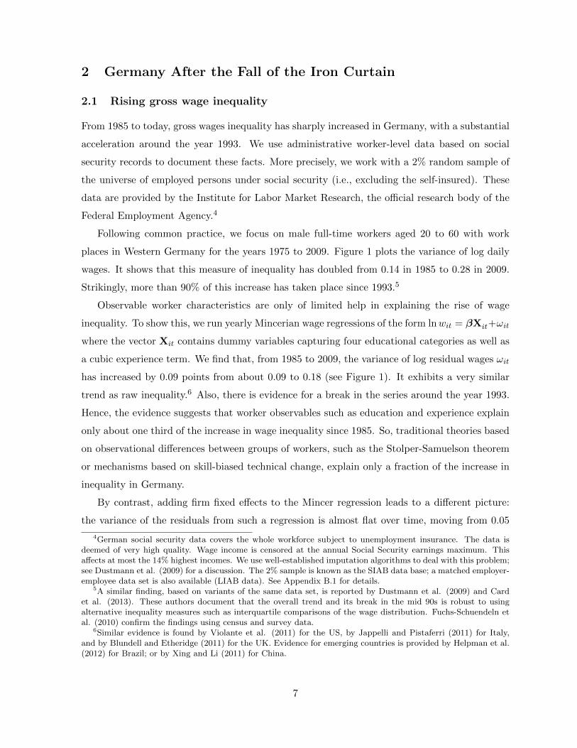
places in Western Germany for the years 1975 to 2009. Figure 1 plots the variance of log daily
wages. It shows that this measure of inequality has doubled from 0.14 in 1985 to 0.28 in 2009.
Strikingly, more than 90% of this increase has taken place since 1993.5
Observable worker characteristics are only of limited help in explaining the rise of wage
inequality. To show this, we run yearly Mincerian wage regressions of the form lnwit = βXit+ωit
where the vector Xit contains dummy variables capturing four educational categories as well as
a cubic experience term. We find that, from 1985 to 2009, the variance of log residual wages ωit
has increased by 0.09 points from about 0.09 to 0.18 (see Figure 1). It exhibits a very similar
trend as raw inequality.6 Also, there is evidence for a break in the series around the year 1993.
Hence, the evidence suggests that worker observables such as education and experience explain
only about one third of the increase in wage inequality since 1985. So, traditional theories based
on observational differences between groups of workers, such as the Stolper-Samuelson theorem
or mechanisms based on skill-biased technical change, explain only a fraction of the increase in
inequality in Germany.
By contrast, adding firm fixed effects to the Mincer regression leads to a different picture:
the variance of the residuals from such a regression is almost flat over time, moving from 0.05
4German social security data covers the whole workforce subject to unemployment insurance. The data isdeemed of very high quality. Wage income is censored at the annual Social Security earnings maximum. Thisaffects at most the 14% highest incomes. We use well-established imputation algorithms to deal with this problem;see Dustmann et al. (2009) for a discussion. The 2% sample is known as the SIAB data base; a matched employer-employee data set is also available (LIAB data). See Appendix B.1 for details.
5A similar finding, based on variants of the same data set, is reported by Dustmann et al. (2009) and Cardet al. (2013). These authors document that the overall trend and its break in the mid 90s is robust to usingalternative inequality measures such as interquartile comparisons of the wage distribution. Fuchs-Schuendeln etal. (2010) confirm the findings using census and survey data.
6Similar evidence is found by Violante et al. (2011) for the US, by Jappelli and Pistaferri (2011) for Italy,and by Blundell and Etheridge (2011) for the UK. Evidence for emerging countries is provided by Helpman et al.(2012) for Brazil; or by Xing and Li (2011) for China.
7
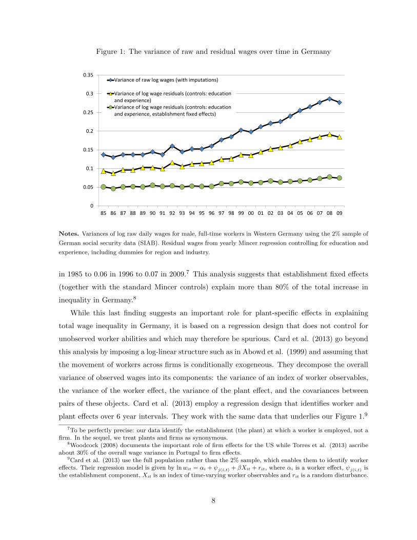
Figure 1: The variance of raw and residual wages over time in Germany
0
0.05
0.1
0.15
0.2
0.25
0.3
0.35
85 86 87 88 89 90 91 92 93 94 95 96 97 98 99 00 01 02 03 04 05 06 07 08 09
Variance of raw log wages (with imputations)
Variance of log wage residuals (controls: educationand experience)Variance of log wage residuals (controls: educationand experience, establishment fixed effects)
Notes. Variances of log raw daily wages for male, full-time workers in Western Germany using the 2% sample of
German social security data (SIAB). Residual wages from yearly Mincer regression controlling for education and
experience, including dummies for region and industry.
in 1985 to 0.06 in 1996 to 0.07 in 2009.7 This analysis suggests that establishment fixed effects
(together with the standard Mincer controls) explain more than 80% of the total increase in
inequality in Germany.8
While this last finding suggests an important role for plant-specific effects in explaining
total wage inequality in Germany, it is based on a regression design that does not control for
unobserved worker abilities and which may therefore be spurious. Card et al. (2013) go beyond
this analysis by imposing a log-linear structure such as in Abowd et al. (1999) and assuming that
the movement of workers across firms is conditionally exogeneous. They decompose the overall
variance of observed wages into its components: the variance of an index of worker observables,
the variance of the worker effect, the variance of the plant effect, and the covariances between
pairs of these objects. Card et al. (2013) employ a regression design that identifies worker and
plant effects over 6 year intervals. They work with the same data that underlies our Figure 1.9
7To be perfectly precise: our data identify the establishment (the plant) at which a worker is employed, not afirm. In the sequel, we treat plants and firms as synonymous.
8Woodcock (2008) documents the important role of firm effects for the US while Torres et al. (2013) ascribeabout 30% of the overall wage variance in Portugal to firm effects.
9Card et al. (2013) use the full population rather than the 2% sample, which enables them to identify workereffects. Their regression model is given by lnwit = αi + ψj(i,t) + βXit + rit, where αi is a worker effect, ψj(i,t) isthe establishment component, Xit is an index of time-varying worker observables and rit is a random disturbance.
8
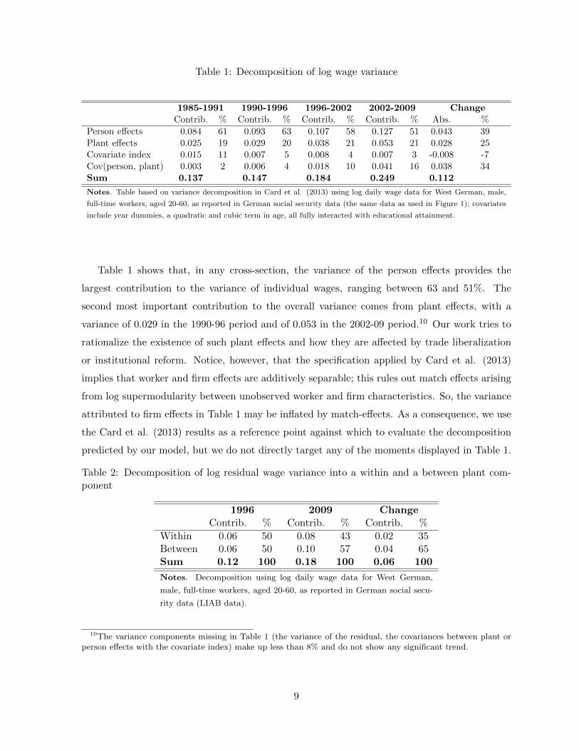
Table 1: Decomposition of log wage variance
1985-1991 1990-1996 1996-2002 2002-2009 ChangeContrib. % Contrib. % Contrib. % Contrib. % Abs. %
Person effects 0.084 61 0.093 63 0.107 58 0.127 51 0.043 39Plant effects 0.025 19 0.029 20 0.038 21 0.053 21 0.028 25Covariate index 0.015 11 0.007 5 0.008 4 0.007 3 -0.008 -7Cov(person, plant) 0.003 2 0.006 4 0.018 10 0.041 16 0.038 34Sum 0.137 0.147 0.184 0.249 0.112
Notes. Table based on variance decomposition in Card et al. (2013) using log daily wage data for West German, male,
full-time workers, aged 20-60, as reported in German social security data (the same data as used in Figure 1); covariates
include year dummies, a quadratic and cubic term in age, all fully interacted with educational attainment.
Table 1 shows that, in any cross-section, the variance of the person effects provides the
largest contribution to the variance of individual wages, ranging between 63 and 51%. The
second most important contribution to the overall variance comes from plant effects, with a
variance of 0.029 in the 1990-96 period and of 0.053 in the 2002-09 period.10 Our work tries to
rationalize the existence of such plant effects and how they are affected by trade liberalization
or institutional reform. Notice, however, that the specification applied by Card et al. (2013)
implies that worker and firm effects are additively separable; this rules out match effects arising
from log supermodularity between unobserved worker and firm characteristics. So, the variance
attributed to firm effects in Table 1 may be inflated by match-effects. As a consequence, we use
the Card et al. (2013) results as a reference point against which to evaluate the decomposition
predicted by our model, but we do not directly target any of the moments displayed in Table 1.
Table 2: Decomposition of log residual wage variance into a within and a between plant com-ponent
1996 2009 ChangeContrib. % Contrib. % Contrib. %
Within 0.06 50 0.08 43 0.02 35Between 0.06 50 0.10 57 0.04 65Sum 0.12 100 0.18 100 0.06 100
Notes. Decomposition using log daily wage data for West German,
male, full-time workers, aged 20-60, as reported in German social secu-
rity data (LIAB data).
10The variance components missing in Table 1 (the variance of the residual, the covariances between plant orperson effects with the covariate index) make up less than 8% and do not show any significant trend.
9
Finally, we decompose the variance of log residual wages into a within-plant and a between-
plant component.11 We do so using the LIAB data set, and report the years 1996 and 2009.
We find that, in 1996, both components were of similar importance for total wage inequality;
in 2009, the relative weight of the within component has decreased to about 43%. Thus, about
two thirds of the total increase in inequality is due to the between component. This is in line
with the recent findings by Bloom et al. (2015) for the US.
The evidence suggests an important role for firm effects. It also shows that a non-trivial share
of the increase in wage inequality is driven by the between-firm component. While Helpman et
al. (2010) analyze the link between trade and the extent of assortative matching, our model
focuses on the the role of firm effects for both between and within firm components of wage
inequality.
2.2 Increasing competition and institutional reform
There is an open debate as to the relative roles of labor market reform, technological change,
product market deregulation, and international trade in explaining the facts described above.
In their empirical work, Autor et al. (2013, 2014) have forcefully argued that exposure to
competition from China has led to higher wage inequality in the US; Dauth et al. (2014) use
similar econometric techniques to show that increased trade with Eastern Europe and China has
also boosted earnings dispersion in Germany. Others such as Dustmann et al. (2014) stress the
role of institutional changes, in particular labor market reforms. These papers cannot always
fully control for other drivers of inequality. Our strategy is to employ a structural equilibrium
model where we have full control over counterfactuals.
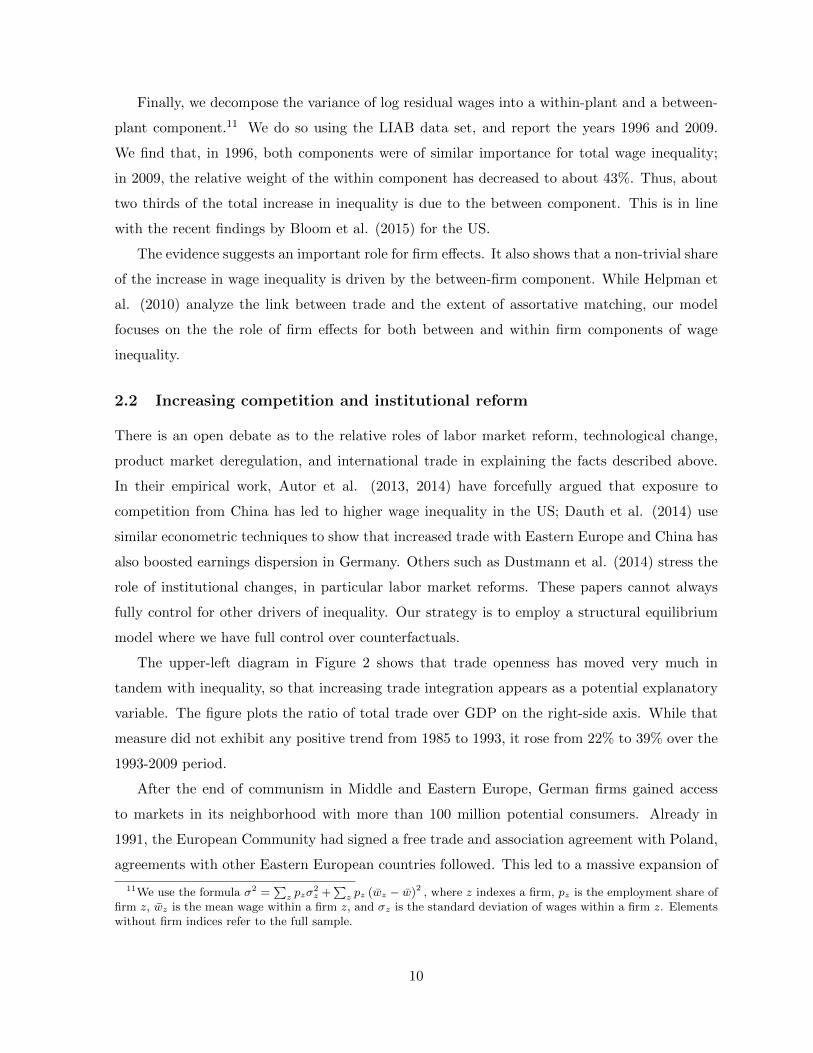
The upper-left diagram in Figure 2 shows that trade openness has moved very much in
tandem with inequality, so that increasing trade integration appears as a potential explanatory
variable. The figure plots the ratio of total trade over GDP on the right-side axis. While that
measure did not exhibit any positive trend from 1985 to 1993, it rose from 22% to 39% over the
1993-2009 period.
After the end of communism in Middle and Eastern Europe, German firms gained access
to markets in its neighborhood with more than 100 million potential consumers. Already in
1991, the European Community had signed a free trade and association agreement with Poland,
agreements with other Eastern European countries followed. This led to a massive expansion of
11We use the formula σ2 =∑z pzσ
2z +
∑z pz (wz − w)2 , where z indexes a firm, pz is the employment share of
firm z, wz is the mean wage within a firm z, and σz is the standard deviation of wages within a firm z. Elementswithout firm indices refer to the full sample.
10
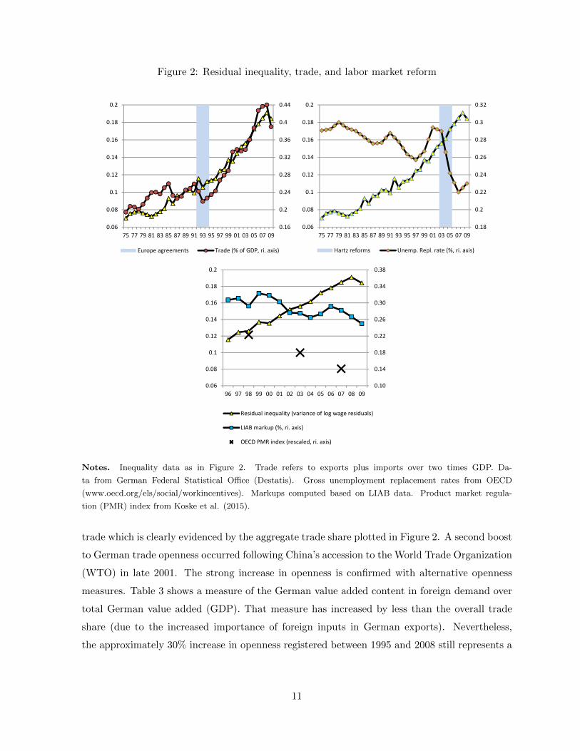
Figure 2: Residual inequality, trade, and labor market reform
Markup PMR
0.31 0.31 0.27 2.230.31 0.34 0.31 0.24 0.22 1.80.24 0.24 0.24
Easternpe
0.10
0.14
0.18
0.22
0.26
0.30
0.34
0.38
0.06
0.08
0.1
0.12
0.14
0.16
0.18
0.2
96 97 98 99 00 01 02 03 04 05 06 07 08 09
Residual inequality (variance of log wage residuals)
LIAB markup (%, ri. axis)
OECD PMR index (rescaled, ri. axis)
0.16
0.2
0.24
0.28
0.32
0.36
0.4
0.44
0.06
0.08
0.1
0.12
0.14
0.16
0.18
0.2
75 77 79 81 83 85 87 89 91 93 95 97 99 01 03 05 07 09
Europe agreements Trade (% of GDP, ri. axis)
0.18
0.2
0.22
0.24
0.26
0.28
0.3
0.32
0.06
0.08
0.1
0.12
0.14
0.16
0.18
0.2
75 77 79 81 83 85 87 89 91 93 95 97 99 01 03 05 07 09
Hartz reforms Unemp. Repl. rate (%, ri. axis)
Notes. Inequality data as in Figure 2. Trade refers to exports plus imports over two times GDP. Da-
ta from German Federal Statistical Office (Destatis). Gross unemployment replacement rates from OECD
(www.oecd.org/els/social/workincentives). Markups computed based on LIAB data. Product market regula-
tion (PMR) index from Koske et al. (2015).
trade which is clearly evidenced by the aggregate trade share plotted in Figure 2. A second boost
to German trade openness occurred following China’s accession to the World Trade Organization
(WTO) in late 2001. The strong increase in openness is confirmed with alternative openness
measures. Table 3 shows a measure of the German value added content in foreign demand over
total German value added (GDP). That measure has increased by less than the overall trade
share (due to the increased importance of foreign inputs in German exports). Nevertheless,
the approximately 30% increase in openness registered between 1995 and 2008 still represents a
11
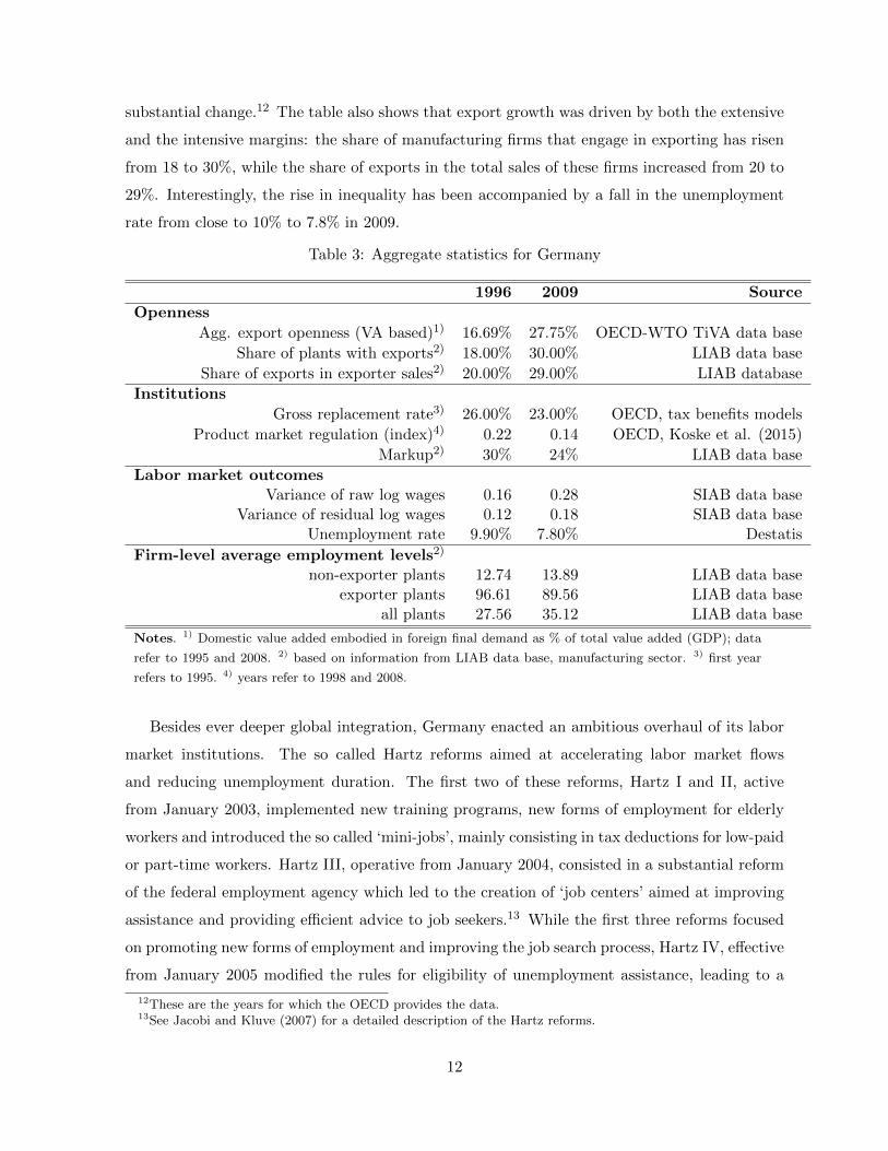
substantial change.12 The table also shows that export growth was driven by both the extensive
and the intensive margins: the share of manufacturing firms that engage in exporting has risen
from 18 to 30%, while the share of exports in the total sales of these firms increased from 20 to
29%. Interestingly, the rise in inequality has been accompanied by a fall in the unemployment
rate from close to 10% to 7.8% in 2009.
Table 3: Aggregate statistics for Germany
1996 2009 Source
Openness
Agg. export openness (VA based)1) 16.69% 27.75% OECD-WTO TiVA data base
Share of plants with exports2) 18.00% 30.00% LIAB data base
Share of exports in exporter sales2) 20.00% 29.00% LIAB database
Institutions
Gross replacement rate3) 26.00% 23.00% OECD, tax benefits models
Product market regulation (index)4) 0.22 0.14 OECD, Koske et al. (2015)
Markup2) 30% 24% LIAB data base
Labor market outcomesVariance of raw log wages 0.16 0.28 SIAB data base
Variance of residual log wages 0.12 0.18 SIAB data baseUnemployment rate 9.90% 7.80% Destatis
Firm-level average employment levels2)
non-exporter plants 12.74 13.89 LIAB data baseexporter plants 96.61 89.56 LIAB data base
all plants 27.56 35.12 LIAB data base
Notes. 1) Domestic value added embodied in foreign final demand as % of total value added (GDP); data
refer to 1995 and 2008. 2) based on information from LIAB data base, manufacturing sector. 3) first year
refers to 1995. 4) years refer to 1998 and 2008.
Besides ever deeper global integration, Germany enacted an ambitious overhaul of its labor
market institutions. The so called Hartz reforms aimed at accelerating labor market flows
and reducing unemployment duration. The first two of these reforms, Hartz I and II, active
from January 2003, implemented new training programs, new forms of employment for elderly
workers and introduced the so called ‘mini-jobs’, mainly consisting in tax deductions for low-paid
or part-time workers. Hartz III, operative from January 2004, consisted in a substantial reform
of the federal employment agency which led to the creation of ‘job centers’ aimed at improving
assistance and providing efficient advice to job seekers.13 While the first three reforms focused
on promoting new forms of employment and improving the job search process, Hartz IV, effective
from January 2005 modified the rules for eligibility of unemployment assistance, leading to a
12These are the years for which the OECD provides the data.13See Jacobi and Kluve (2007) for a detailed description of the Hartz reforms.
12
reduction in average levels and duration of unemployment benefits.
In order to evaluate the effects of the first three reforms, Fahr and Sunde (2009) and Hertweck
and Sigrist (2012) provide an estimation of the matching function and of its changes after the
reforms. Their main result shows that the reforms, especially Hartz III, produced a substantial
improvement of the efficiency of the matching process in Germany. Fahr and Sunde (2009) find
that the flows from unemployment to employment accelerated by 5-10%, corresponding to a
reduction in the average unemployment duration of the same order of magnitude. In the upper-
right diagram in Figure 2, we report OECD estimates of gross unemployment replacement rates
for Germany, which document a decline from a level of 29% in 2001 to 23% in 2009.14 However,
the generosity of unemployment benefits has been on a downward trend even before.15
Finally, like many other OECD countries, Germany has substantially deregulated its product
market. According to information from the OECD’s product market regulation (PMR) data
base, from 1998 to 2008 the index of PMR intensity has fallen from 0.22 to 0.14;16 about three
quarters of this decline happened from 1998 to 2003 (Koske et al., 2015). The lower diagram
in Figure 2 provides an illustration. This index is based on several measures of product market
regulations broadly grouped in state control indicators (e.g. scope of public enterprises, price
controls), barriers to entrepreneurship (e.g. administrative and legal burdens, barriers to entry),
and barriers to trade (e.g. barriers to FDI, discriminatory procedures against foreign firms).
Decomposing the sources of regulatory reforms for Germany shows that the liberalization push
came mostly from the reduction of state controls and of barriers to entrepreneurship.17 The
deregulation of the product markets and increased foreign competition may have lowered profit
margins of German firms. The lower diagram in Figure 2 plots proxies for markups derived from
the LIAB data set. Operating profits are calculated as revenues minus total costs, where total
costs are made up of the wage bill plus material inputs. Markups are defined as the share of
operating profits in revenues. Quite strikingly, some volatility notwithstanding, markups have
trended downwards from about 31% in 1996 to about 25% in 2009.
14See the data on www.oecd.org/els/social/workincentives.15Another important change in labor market institutions in those years is the reduction in collective bargaining
coverage which followed German reunification. The German LIAB data show that about 80% of all firms werecovered by industry agreements in 1996; this share declined to about 60% in 2009, with most of the declineoccurring prior to 2005. We do not study this institutional change here; for an empirical analysis of the linksbetween the fall in collective bargaining and wage inequality in Germany see Dustmann et al. (2009) and Cardet al. (2013).
16To ease the presentation, the original OECD index was rescaled using the factor 0.1.17See Wolf et al. (2015) Table 2. Importantly, that measure is much wider in scope than any index of trade
openness.
13
3 Model
We propose a continuous time framework that brings together the Melitz (2003) trade model
with the directed search approach of Kaas and Kircher (2015). Trade between two symmetric
countries is subject to variable and fixed costs, while the labor market is characterized by search-
and-matching frictions and convex adjustment costs.18 Workers are homogenous but firms are
heterogenous with respect to their productivity.
3.1 Model setup
Final output producers. Consumer preferences are linear over a single final output good Y
that is produced, under perfect competition, according to an aggregate CES production function
Y = M−1
σ−1
[∫ω∈Ω
y (ω)σ−1σ dω
] σσ−1
, σ > 1 , (1)
where the measure of the set Ω is the mass M of available varieties of intermediate inputs,
ω denotes such an input, y (ω) is the quantity of the input used, and σ is the elasticity of
substitution across varieties. The term M−1/(σ−1) neutralizes the scale effect due to love of
variety otherwise present in CES aggregator functions.19 The price index dual to (1) is given
by
P ,
[1
M
∫ω∈Ω
p (ω)1−σ dω
] 11−σ
, (2)
and is used as the numeraire, i.e., P = 1. Then aggregate income is simply equal to Y. With
these assumptions, demand for an intermediate good ω is given by the isoelastic inverse demand
function
y (ω) =Y
Mp (ω)−σ . (3)
Intermediate input producers. Producers of intermediate goods operate under monopolis-
tic competition. Payment of an entry fee of fE/(r + δ) allow firms to draw their time-invariant
productivity levels z (ω) from a sampling distribution with c.d.f. G (z). Productivity remains
constant over a firm’s lifetime, but employment `a (ω) is a function of firm age a. Output is
18We opt for a symmetric framework, mostly for the sake of tractability and to avoid simplifying but problematicassumptions (such as the introduction of a linear outside sector). Trade costs have fallen symetrically; hence, oursetup comes with little loss of generality.
19This avoids a counterfactual negative correlation between the unemployment rate in autarky and the size ofthe country (labor supply). With trade and symmetric countries, this counterfactual implication is maintainedon the world level. See Felbermayr, Prat, and Schmerer (2011) for a discussion of the case of positive gains fromvariety.
14
given by a linear production function
y (`a;ω) = z (ω) `a (ω) . (4)
Due to monopolistic competition, each firm produces a unique variety; the dependence of z and
optimal ` on ω is understood and suppressed in the present section.
Firms need to pay a flow fixed cost f in order to operate domestically and another flow fixed
cost fX > f if they are present on the export market. Each unit of production shipped abroad is
subject to an iceberg-type variable trade cost τ ≥ 1. As will be shown later, due to the presence
of fixed market access costs in equilibrium only firms with sufficiently high productivity levels
z ≥ z∗D find it profitable to operate, and only the most productive firms featuring z ≥ z∗X > z∗D
will also decide to export.
Revenues from exporting are pXyX/τ and producers face the same demand (3) for domestic
and foreign sales. Thus prices and quantities in the domestic and foreign markets satisfy:
pX(z) = τpD(z) and yX(z) = τ1−σyD(z). Total revenues are therefore given by
R(`a, Ia; z) =
[Y
M
(1 + Iaτ1−σ)] 1
σ
(z`a)σ−1σ , (5)
where Ia is an indicator function that takes value 1 when the firms serves the foreign market
and 0 otherwise.
Directed job search. Labor is the only factor of production. Transactions in the labor market
are segmented over a continuum of submarkets, each indexed by its ratio of open vacancies to job
seekers θ = V (θ) /S (θ).20 The matching function in each submarket features constant returns
to scale. Thus, if we let q (θ) denote the vacancy filling rate (with ∂q (θ) /∂θ < 0), θq (θ) is the
rate of finding a job (with ∂ [q (θ) θ] /∂θ > 0). We use η , −q′ (θ) θ/q (θ) to denote the constant
elasticity of the filling rate with respect to θ.
Firms are destroyed at the time-invariant Poisson rate δ. Workers and firms separate at the
natural attrition rate χ. Both δ and χ are treated as exogenous. New firms are continuously
created. They differ with respect to their innate productivity levels but start their lives equally
small. They grow smoothly over time due the presence of convex adjustment costs, with growth
rates depending on productivity. This leads to a cross-section of firms whose employment levels
20V (θ) and S (θ) denote the number of open vacancies and job seekers in the submarket with tightness θ. Whenwe refer to ‘labor market tightness’, we take the perspective of searching workers. A lower value of θ, thus, reflectsa tighter labor market.
15
depend on both age and productivity.
We assume that search is directed and that firms have the ability to commit. They post
contracts which stipulate wage rates w for any point in time at which the firm operates. Since
workers are risk neutral, they do not have preferences over the timing of payments as long as
they yield the same discounted sum. Thus we simplify matters by considering that workers are
offered a constant income stream. This choice of wage profile is also without loss of generality
from the firm’s standpoint: it does not affect its optimization problem because promised wages
are sunk and, as such, do not affect future decisions. By committing to a wage, firms decide in
which submarket θ they want to recruit and how many vacancies they want to create. Workers
have information about each submarket prior to their search and use it to select the submarket in
which they apply. Hence conditions across submarkets must be such that workers are indifferent.
It is convenient to derive first the reservation wage as well as the indifference condition
relating wages across submarkets. Workers’ asset values satisfy the following conditions
rE (w) = w + (δ + χ) [U − E (w)] ,
rU = b+ θq(θ) [E (w)− U ] ,
where the interest rate is denoted by r and unemployment benefits (the value of leisure) by b.
The flow value of employment is rE (w). By definition, the reservation wage wr is such that
rU = wr.
Substituting E (w) out of the above system and using wr = rU , we obtain
wr = b+ θq(θ)
[w(θ)− wrr + δ + χ
]︸ ︷︷ ︸
,ρ
. (6)
The variable ρ denotes the premium commended by workers over the flow value b of being
unemployed. The expression can be rearranged so as to define the indifference condition for
workers across submarkets w (θ) = wr + ρ (r + δ + χ) /θq(θ). The condition above shows the
positive relationship between wages and the vacancy filling rate typical of directed search models
(e.g., Moen, 1997; Acemoglu and Shimer, 1999). Conversely, wages and the job finding rate are
negatively related: workers search in submarkets with low wages only if they have a higher
probability to find a job. As wages approach the value of leisure, the gains derived from being
employed vanish and the arrival rate of jobs diverges to infinity.
16

3.2 Firm policies
Consider a firm of age a. Its value Π depends on two state variables: the current level of
employment `a and the cumulated wage bill Wa ,∫ a
0 e−χ(a−s)q(θs)vsw (θs) ds. Firms face the
adjustment cost function C (v) , which is an increasing and strictly positive function of the
number of vacancies posted. They solve the following problem:
Π (`a,Wa; z) , maxθs,vs,Is
∫ ∞a
e−(r+δ)(s−a) [R (`s, Is; z)−Ws − C(vs)− f − IsfX ] ds
s.t. ˙s = q(θs)vs − χ`s; (7)
Ws = q(θs)vsw (θs)− χWs; (8)
w (θs) = wr +ρ
θsq(θs)(r + δ + χ) . (9)
The firm chooses the labor market segment θs in which it wishes to recruit, and the mass vs of
new vacancies to be created at age s. It also makes an export decision, i.e., it sets the export
dummy Is to either zero or one. The firm’s problem is subject to three constraints. The first
constraint (equation (7)) represents the law of motion of firm size: vacancies are filled at the rate
q (θs) and jobs are destroyed at the attrition rate χ. Equation (8) describes the law of motion
of the cumulated wage bill: at each instant, random separation shocks lower the wage bill by
the amount χWs, while new hires q(θs)vs, who are paid the wage w (θs) , add to the total wage
bill. Equation (9) is a reformulation of the indifference condition (6) derived above.
As explained before, the cumulated wage bill W does not affect future decisions because it
is sunk. Expected profits can therefore be decomposed as follows
Π (`a,Wa; z) = Ψ (`a; z)−Wa
r + δ + χ− f
r + δ,
which allows us to write the value of the firm as the solution of the following Hamilton-Jacobi-
Bellman (HJB) equation
(r + δ) Π (`a,Wa; z) = maxva,θa,Ia
R (`a, Ia; z)−Wa − C(va)− f − IafX +
∂Ψ (`a, Ia; z)∂`a
˙a −
Wa
r + δ + χ
.
(10)
Eliminating the terms including W and replacing the law of motions (7) and (8) yields
(r + δ) Ψ (`a; z) = maxva,θa,Ia
R (`a, Ia; z)− C(va)− IafX+∂Ψ(`a,Ia;z)
∂`a[q(θa)va − χ`a]− w(θa)
r+δ+χq(θa)va
. (11)
17
Recruitment policy. The policy functions are derived by maximizing the simplified Bellman
equation (11). Remember that, in each period, a firm chooses the tightness of the submarket in
which it recruits along with the number of vacancies. The first order condition with respect to
v readsC ′ (va)
q(θa)=∂Ψ (`a, Ia; z)
∂`a− w (θa)
r + δ + χ. (12)
Quite intuitively, the expected marginal cost of hiring an additional worker, C ′ (va) /q(θa),
should be equal to the worker’s shadow value, ∂Ψ (`a; z) /∂`a, minus the discounted wage bill,
w (θa) / (r + δ + χ) .
Maximizing the objective function with respect to θ yields
∂Ψ (`a, Ia; z)∂`a
q′(θa) = w′ (θa)q(θa)
r + δ + χ+ w (θa)
q′(θa)
r + δ + χ. (13)
By varying θ, the firm affects the vacancy filling rate and thus the extent to which it can benefit
from the shadow value of a filled vacancy. At the same time, changing θ also changes expected
wage costs, both because a different choice of labor market segment θ requires the posting of a
different wage and because variation in the job fill rate implies variation in the likelihood that
the posted wage actually needs to be paid. In equilibrium, the two marginal effects must be
identical. Combining (12) and (13), we obtain
θa =1− ηη
ρ
C ′ (va), (14)
where η denotes the elasticity of the matching function.
The relationship between θa and va does not depend on the (endogenous) export status Ia.
The sign of the relationship is determined by the curvature of the recruitment cost function.
When vacancy costs are convex, i.e., C ′′ (va) > 0, firms wishing to post more vacancies search in
labor markets characterized by higher tightness (lower θa). Since wages are decreasing in market
tightness, we can conclude that firms with larger adjustment needs (higher va) pay higher wages.
Thus, if vacancy costs are convex, the model replicates the positive empirical correlation between
firm growth and wages paid to new hires. This result is intuitive: given that recruitment costs
increase over-proportionately, firms that wish to hire many workers find it profitable to post
higher wages in order to raise their job filling rates.
Proposition 1 (Wage-Size Link) If recruitment costs are strictly convex, firms wishing to
expand employment faster post higher wages. If, additionally, recruitment costs are isoelastic,
firms with larger steady state employment levels create more vacancies and post higher wages.
18
These effects are bigger, the greater the degree of convexity. Conversely, if recruitment costs are
strictly concave, faster growing and larger firms post lower wages.
Proof. The first part of the Proposition is shown in the text. To prove the second part, note
that steady state employment of the firm is given by ¯= q(θ)v/χ and, hence,
(∂ ¯/∂v
) (v/¯)
=
−η(∂θ/∂v
) (v/θ)
+ 1. When the cost function has a constant elasticity C ′(v)v/C(v) ≡ α, (14)
implies(∂θ/∂v
) (v/θ)
= 1−α, and so(∂ ¯/∂v
) (v/¯)
= 1− η (1− α) > 0. The sign follows when
C (v) is convex, i.e., α > 1.
In order to capture the well documented correlation between firm size and wages, we will
hereafter restrict our attention to convex cost functions.21 The empirical literature supports this
assumption. Direct empirical evidence is provided by Merz and Yashiv (2007), who estimate
a structural model using US data and show that both labor and capital adjustment costs are
strongly convex. Similarly Manning (2006) using UK data finds evidence of convex labor ad-
justment costs. Besides these findings providing direct support to the convexity assumption,22
Davis et al. (2013) find that US firms grow through a smooth process and that, as predicted by
our model, faster growing firms fill their vacancies quicker.
Export status. The decision to export depends not only on the productivity, but also on the
size (and, thus, on the age) of the firm. Young productive firms start small but gradually build
up their work force until exporting a share of their output covers the fixed costs required to
access the foreign market. They choose the exporting status that maximizes current revenues
net of fixed costs,
Ia(z) = arg maxIa∈0,1
R (`, Ia; z)− IafX .
The solution to this problem implies that there exists a size threshold `X (z) , which makes firms
indifferent between exporting and not exporting
`X (z) =1
z
fX(YM
) 1σ
[(1 + τ1−σ)
1σ − 1
]
σσ−1
, (15)
so that firms featuring `a (z) > `X (z) will be exporters. Forward-looking future exporters
build up employment before they reach the age aX(z) , inf a : Ia (z) = 1 at which they enter
21If C′′ (va) = 0, there is no link between the number of vacancies that a firm wishes to post and the labormarket it selects, and, by (6), there would not be any wage dispersion.
22Shimer (2010) proposes a theoretical microfundation of convexity in labor adjustment costs. With concaverevenues functions, the opportunity cost of reallocating workers from production tasks to recruitment tasks isconvex in the size of the adjustment.
19
the foreign market. Optimal hiring ensures that employment grows smoothly over time. In
particular, recruitment intensity does not jump when a firm starts exporting. By contrast, the
share of domestic sales in total sales falls discretely at age aX to make room for exports.
Note that the critical size `X (z) is decreasing in the firm’s productivity level z. As we will
see below, firms with higher productivity have higher employment growth rates at all ages. This
means that they start exporting earlier than less efficient firms. The property of our model,
that export status is a function of productivity z and age a rationalizes the overlap in the
productivity distribution of exporters and non-exporters observed in the data (e.g. Roberts and
Tybout, 1997; Bernard et al., 2003).
Dynamic conditions. We now derive the dynamic conditions governing the evolution of firm
size. The following parametric assumptions provide tractability:
Assumption 1 Vacancy costs are isoelastic, C (v) = vα, with α > 1.
Assumption 2 The matching function is Cobb-Douglas, q(θ) = Aθ−η, with η ∈ (0, 1).
Solving the HJB equation (11), we obtain the equilibrium employment path and the dynamics
of firm size and wage distribution.
Proposition 2 (Firm Employment Growth) Under Assumptions 1 and 2, the optimal em-
ployment schedule of any given firm satisfies
(˙a + χ`aξ0
)ξ1 (r + δ + χ− ξ1
¨a + χ ˙
a
˙a + χ`a
)=η
ρ[R1 (`a, Ia; z)− wr] , (16)
with ξ0 , A1+1/ξ1
[(1η − 1
)ρα
] 1α−1
> 0 and ξ1 , 1−ηη+1/(α−1) > 0. The optimal solution to (16) is
pinned down by the boundary conditions (i) `0 = 0, and (ii) lima→∞ `a(z) = ¯(z) with23
(χ¯(z)
ξ0
)ξ1=η
ρ
[R1
[¯(z) , I
(¯(z) , z
); z]− wr
r + δ + χ
]. (17)
The boundary condition for firms that eventually become exporters is given by the smooth pasting
condition: lim`a→`
X−z
˙a (z) = lim
`a→`X+z
˙a (z) .
Proof. See Appendix A.1.
23A solution always exists and is unique since the LHS is increasing in ¯and has function values in (0,∞), whilethe RHS is decreasing and takes values in [−wrη/ρ (r + δ + χ) ,∞).
20
According to (17), marginal revenues R1 (·) converge to a limit that is higher than the
reservation wage wr. This is because workers have a strictly positive turnover rate χ > 0 and so
need to be replaced through costly recruitment. This drives a wedge between the opportunity
cost of employment and the productivity of the marginal worker.
Equation (17) also shows that more productive firms converge to larger sizes (since R1(.) is
increasing in z). Moreover, firms that will end up being exporters have larger size conditional
on age than non exporters. Hence, while the firm size distribution is continuous in firm age a, it
exhibits a discontinuity in the productivity space, as firms with z ≥ z∗X will be larger at all ages.
Ceteris paribus, asymptotic firm sizes are lower the higher the value of unemployment benefits,
or the less efficient the matching process. Finally, firms converge to larger sizes the bigger σ is,
since this reduces monopoly power.
To characterize the equilibrium wage policy for each firm, notice that the equilibrium job
finding rate θq(θ) can be expressed as([
˙a(z) + χ`a(z)
]/ξ0
)−ξ1.24 Then, the worker indifference
condition (9) implies that
wa (z) = wr +
(˙a(z) + χ`a(z)
ξ0
)ξ1(r + δ + χ) (wr − b). (18)
By equation (7), this expression shows that search frictions lead to a markup of wages above
the reservation wage and that this markup is proportional to the adjustment needs of a firm
since qa (z) va (z) = ˙a(z) + χ`a(z). Equation (18) displays a growth and a size premium. A
higher efficiency of the search technology lowers those premia, as higher A implies high ξ0. A
higher degree of convexity α in the adjustment cost function leads to a higher value of ξ1 and
makes wages more responsive to firms’ adjustment needs. The higher the effective discount
rate r + δ + χ, the higher the premium as firms find it even more worthwhile to post higher
wages to fill vacancies faster. International trade affects the distribution of wages by affecting
the distribution of firm-level adjustment needs. As we will see below, lower trade costs lead to
a more skewed distribution of firm sizes and growth rates, thereby altering the distribution of
˙a(z) + χ`a(z) and hence that of wages.
Note that (18) describes wages of workers hired at a firm of age a. However, the firm employs
workers hired throughout its history, possibly at different wages. This generates within-firm wage
inequality: as adjustment needs change over time so do wages paid to new hires.
24See equation (41) in the Appendix.
21
3.3 General Equilibrium
Having characterized firms’ policies, we now close the model. We need to determine the equi-
librium productivity cutoffs z∗D and z∗X , along with aggregate output and the unemployment
rate. Recalling that new firms draw their productivity from the distribution G (z), the equilib-
rium density of the productivity distribution is µ (z) , g (z) / [1−G (z∗D)] for all z ≥ z∗D; and
the share of exporting firms is given by % < 1. Average output per firm Y/M is given by the
accounting identity
Y
M=
[1
1 + %
∫ ∞z∗D
(∫ ∞0
(1 + Ia;zτ
1−σ) 1σ (z`a(z))
σ−1σ δe−δada
)µ(z)dz
] σσ−1
, (19)
where employment `a(z) of a firm of age a and productivity z is consistent with the optimality
conditions described in Proposition 2.25 Average output Y/M is a shifter of the revenue function
(5), and thus a key equilibrium object driving firm behavior.
In contrast to Melitz (2003) (or to the one-period model discussed below), profits are not
log-linear in productivity. Thus, the usual result that the two cutoffs z∗X and z∗D are multiples of
each other does not hold anymore. Instead, we have to directly compute revenues and verify that
the zero cutoff profit (ZCP) conditions, which ensure that the marginal domestic and exporting
firms exactly break even, are satisfied. The same holds for the free entry (FE) condition which
ensures that entry of new firms occurs until expected profits are exactly identical to the entry
costs fE/(r + δ).
For given recruitment policies, discounted profits are easily computed reinserting equations
(11) and (12) into the definition of Π (·) to obtain
Π (0, 0; z) =1
r + δ
[C ′ (v0 (z))
q(θ0 (z))˙0 (z)− C(v0 (z))− f − e−(r+δ)aX(z)fX
](20)
=1
r + δ
[(α− 1) v0 (z)α − f − e−(r+δ)aX(z)fX
].
where aX(z) , inf a : Ia (z) = 1 is the age at which firm z enters the foreign market.26 Equation
(20) enables us to solve for the domestic cutoff z∗D as the zero cutoff profit condition (ZCP)
reads Π (0, 0; z∗D) = 0 : startups have zero employment and thus no promised wage, i.e., `0 =
W0 = 0. In turn, the export productivity cutoff z∗x is determined by the condition, z∗X =
infz : ¯(z) ≥ `X(z)
, according to which the marginal exporter is the least productive firm
25The expression for aggregate employment takes into account that firms are destroyed each period at thePoisson rate δ.
26When the firm always remains a domestic producer, ax = +∞ and the last term in (20) vanishes.
22

reaching the export threshold size `X(z) defined in (15). The free entry condition is satisfied
when (1−G (z∗D))∫∞z∗D
Π (0, 0; z)µ(z)dz = fE/ (r + δ). Since ρ = wr − b, the ZCP and the
free entry condition along with (19) provide us with three equations for the three unknowns
Y/M,wr, z∗D . The final closure of the model requires the determination of the mass of firms
M and the unemployment level. Since v(ω)/θ(ω) job seekers are needed to meet the recruitment
needs of firm ω, aggregating over all firms we find that the aggregate number of job seekers reads
S =M
1 + %
∫ ∞z∗D
(∫ ∞0
va(z)
θa(z)δe−δada
)µ(z)dz. (21)
Aggregate employment L can be computed in a similar way to obtain the equilibrium rate of
unemployment U = S/(S + L) and, assuming an inelastic labor supply, the mass of firms such
that S + L equals the size of the population.
4 A One-Period Variant of the Model
We have seen that the effect of international trade on the distribution of wages is driven by the
distribution of firms’ hiring needs. With convex adjustment costs, firms smooth their recruitment
over time. Thus, a dynamic perspective is crucial for a quantitative assessment of the model.
However, to build intuition, we analytically illustrate key model mechanisms using a framework
in which firm adjustment happens within one single period.
4.1 Problem of the firm
Besides assuming that firms adjust within one period, the other deviations from the setup of
Section 3 is to set the value of leisure b to zero. The timing is such that at the beginning of the
periods all workers look for a job. Search is as described in the previous section. Thus, at the
end of the period, a fraction θq (θ) of workers in a given submarket is employed and produces
output. There is no discounting within the period. The expected wage income of a job seeker
in market θ is given by W = θq (θ)w (θ) so that we obtain the indifference condition
w (θ) =W
θq (θ), (22)
which is the counterpart of (9). As in the dynamic model, wages are a negative function of
tightness as workers trade off a higher employment probability against a lower wage.
Firms post vacancies and wages at the beginning of the period; they fill the share q (θ) of
23
the announced jobs, and their end of period employment is ` = q (θ) v. Firm revenues are again
given by (5). Inserting the worker indifference condition and substituting for `, the problem of
the firm reads
π (z) = maxθ,v,I
R (q(θ)v, I; z)− W
θv − C (v)− f − IfX . (23)
The first-order condition with respect to v yields R` (·) q(θ) = W/θ+C ′ (v) and the one with
respect to θ yields R` (·) q′(θ) = −W/θ2. Together these first order conditions imply
θ =1− ηαη
v1−αW, (24)
which is identical to condition (14) in the dynamic model (with W being replaced by ρ = wr−b).
Firms posting more vacancies choose lower levels of θ (i.e., higher market tightness) and therefore
post higher wages. Since ` = q (θ) v, larger firms pay higher wages.
4.2 Distribution of wages across firms
Keeping Assumptions 1 and replacing Assumption 2 by q(θ) = minAθ−η, 1
with η ∈ (0, 1),
we now characterize the distributions of wages, employment and profits.27 We relate variables
across submarkets with the help of a representative firm whose productivity z is such that its
optimal price in the non-exporting sate equals one, i.e., pD(z) = 1. Notice that firms with
productivity z can actually be exporters. Hence, the associated variables ˜, θ and profits π are
constructs which are not necessarily observed in equilibrium. We will alternatively refer to z as
the productivity of the representative firm or average productivity. As shown in Appendix A.2,
this normalization allows us to derive the following wage schedule:
lnw (z) = ln
(η (σ − 1)
σ
)+
(σ − 1− βσ − 1
)ln z︸ ︷︷ ︸
Productivity effect
+β
σ − 1ln z︸ ︷︷ ︸
Avg. efficiency
+ (σ − 1− β) ln(1 + I(z)τ1−σ)︸ ︷︷ ︸
Export status effect
,
(25)
where β is a combination of parameters defined in (49). Since β ∈ (0, σ − 1), log-wages are
increasing in firm productivity. The elasticity of wages with respect to z is constant and equal
to 1 − β/ (σ − 1) . That elasticity is declining in α, the degree of convexity of the adjustment
cost function. In the absence of search frictions, η = 1, or with linear adjustment costs, α = 1,
we have β = σ − 1. Then the wage schedule collapses to lnw (z) = ln ([σ − 1] /σ) + ln z and
27We will focus on equilibria where θq (θ) < 1 in all submarkets.
24

wage dispersion disappears.
The wage schedule has two other components. First, when the efficiency of the representative
firm z increases, the labor market becomes more competitive, and all firms must pay higher
wages. Second, in order to serve the export market, exporting firms are required to reach a
higher equilibrium size. This gives rise to an export wage premium as firms grow to a larger
size by posting higher wages.
4.3 Equilibrium
Domestic and export market entry. Profits net of fixed costs are log-linear in z; see
Appendix A.3 for a proof. More precisely, taking the ratio of operating profits of firm z and of
firm z yields
π (z) + f + I (z) fX =(1 + I (z) τ1−σ)β/(σ−1)
(zz
)β[π + f ] . (26)
Evaluating (26) for the marginal domestic producer z∗D yields the zero cutoff profit (ZCP)
condition
(ZCP ) : π = f[(z (z∗D) /z∗D)β − 1
], (27)
where we account for the dependence of z on z∗D through
z (z∗D) =
[1
1 + %
∫ ∞z∗D
zβ[1 + I(z)τ1−σ]β/(σ−1)
µ (z) dz
]1/β
; (28)
see Appendix A.3 for details. In the absence of search frictions, we would have β = σ−1 and our
ZCP would be identical to that in Melitz (2003). By contrast, in our model there is no ZCP for
exporters. We identify the export cutoff z∗X by using the indifference condition π (z∗X , I = 0) =
π (z∗X , I = 1) . Without loss of generality, one can view the indifferent firm z∗X as serving the
domestic market only. Using (26) ,we obtain
z∗Xz∗D
=
(fXf
)1/β [(1 + τ1−σ)β/(σ−1) − 1
]−1/β≥ 1 . (29)
The two cutoffs are positively related in equilibrium and, as one might expect, the productivity
premium of the marginal exporter z∗X/z∗D is increasing in export fixed costs fX relative to
domestic fixed costs f , and in the iceberg trade factor τ .28
28In the absence of labor market frictions or convex adjustment costs (i.e., η = 1 or α = 1, which both imply
β = σ − 1), the relationship collapses to z∗X/z∗D = (f/fX)−1/(σ−1) τ as in the standard Melitz (2003) model.
25

Free entry condition. The free entry condition ensures that entry occurs until expected
profits are exactly identical to the entry costs fE , hence E [π (z)] = fE/ [1−G (z∗D)] . In equation
(61) of Appendix A.4, we show how expected profits E [π (z)] and profits of the representative
firm π are connected. This allows us to write the following free entry (FE) condition,
(FE) : π =fE + 1−G [z∗X (z∗D)] (fX − f)
2−G(z∗D)−G
[z∗X(z∗D)] . (30)
Product market equilibrium. Using the ZCP condition and the free entry condition (30),
we can now determine product market equilibrium in (π, z∗D)−space. Existence of an equilibrium
is guaranteed if fX < fE and σ > 1 + α.
Proposition 3 (Equilibrium) If fX < fE and σ > 1 + α, the ZCP condition (27) and the
free entry (FE) condition (30) uniquely determine the domestic cutoff z∗D. The export cutoff z∗X
and the productivity of the representative firm z follow from equations (29) and (28).
Proof. See Appendix A.5.
Value of search and welfare. Since W is average labor income and we have normalized the
price index P = 1, the value of search W is a measure of welfare. Using the profit function and
the ZCP condition (27) , one obtains
W =
[K
fzγ (z∗D)β
] 1−ηη
α−1α
, (31)
where γ, β, and K are all positive constants29. So, an increase in the productivity of the marginal
domestic producer and/or of the representative firm raises the value of search. Quite intuitively,
as firms become more efficient, the zero cutoff profit and free entry conditions are reestablished
through an increase in labor costs.
4.4 The impact of trade liberalization
The selection effect. In a first step, we study the effect of lower τ on the productivity of the
representative firm, z. Under the conditions stated in Proposition 3, the FE locus shifts down.
To pin down the shift of the ZCP curve, however, a parameter restriction is needed since the
effect of τ on z is generally ambiguous.
29See equations (49), (57) and (58) in the Appendix.
26
Proposition 4 (Selection) Under the assumptions that firms draw their productivity from a
Pareto distribution and that fX > f, trade liberalization has an unambiguously positive effect on
the domestic cutoff z∗D and z.
Proof. See Appendix A.8.
Trade liberalization expands the market size of productive firms who can take advantage
from easier access to the foreign market. It also hurts less productive firms, whose revenues
may fall due to increased competition by efficient foreign competitors. As a consequence, less
efficient firms shut down, while more efficient firms expand. In line with Melitz (2003), this
selection effect drives up the productivity z of the representative firm as long as the additional
output share lost in iceberg costs does not outweigh the productivity gains at the factory gate.
The reallocation of labor towards more efficient firms increases the value of search. This
is easily established considering the ZCP condition π (z∗D; z,W ) = 0. Equation (50) in the
appendix implies that π (z∗D) is strictly decreasing in W and strictly increasing in both z and
z∗D. Since a reduction in τ raises the productivity of the representative and marginal firms, W
has to increase until the ZCP is satisfied again.
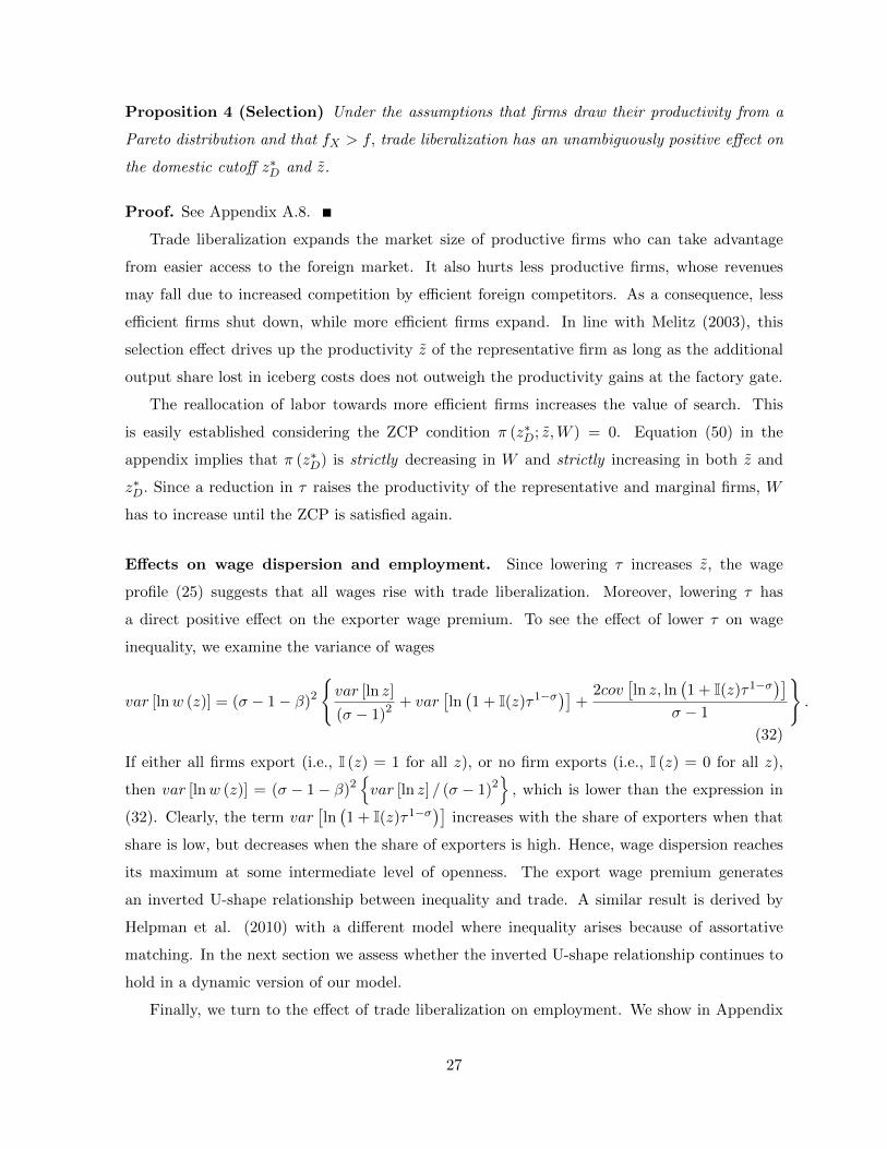
Effects on wage dispersion and employment. Since lowering τ increases z, the wage
profile (25) suggests that all wages rise with trade liberalization. Moreover, lowering τ has
a direct positive effect on the exporter wage premium. To see the effect of lower τ on wage
inequality, we examine the variance of wages
var [lnw (z)] = (σ − 1− β)2
var [ln z]
(σ − 1)2 + var[ln(1 + I(z)τ1−σ)]+
2cov[ln z, ln
(1 + I(z)τ1−σ)]
σ − 1
.
(32)
If either all firms export (i.e., I (z) = 1 for all z), or no firm exports (i.e., I (z) = 0 for all z),
then var [lnw (z)] = (σ − 1− β)2var [ln z] / (σ − 1)2
, which is lower than the expression in
(32). Clearly, the term var[ln(1 + I(z)τ1−σ)] increases with the share of exporters when that
share is low, but decreases when the share of exporters is high. Hence, wage dispersion reaches
its maximum at some intermediate level of openness. The export wage premium generates
an inverted U-shape relationship between inequality and trade. A similar result is derived by
Helpman et al. (2010) with a different model where inequality arises because of assortative
matching. In the next section we assess whether the inverted U-shape relationship continues to
hold in a dynamic version of our model.
Finally, we turn to the effect of trade liberalization on employment. We show in Appendix
27
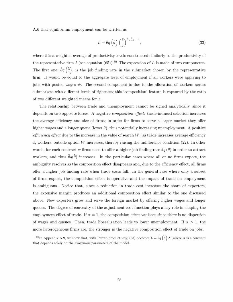
A.6 that equilibrium employment can be written as
L = θq(θ)( z
z
)β σσ−1−1
, (33)
where z is a weighted average of productivity levels constructed similarly to the productivity of
the representative firm z (see equation (65)).30 The expression of L is made of two components.
The first one, θq(θ)
, is the job finding rate in the submarket chosen by the representative
firm. It would be equal to the aggregate level of employment if all workers were applying to
jobs with posted wages w. The second component is due to the allocation of workers across
submarkets with different levels of tightness; this ‘composition’ feature is captured by the ratio
of two different weighted means for z.
The relationship between trade and unemployment cannot be signed analytically, since it
depends on two opposite forces. A negative composition effect : trade-induced selection increases
the average efficiency and size of firms; in order for firms to serve a larger market they offer
higher wages and a longer queue (lower θ), thus potentially increasing unemployment. A positive
efficiency effect due to the increase in the value of search W : as trade increases average efficiency
z, workers’ outside option W increases, thereby raising the indifference condition (22). In other
words, for each contract w firms need to offer a higher job finding rate θq (θ) in order to attract
workers, and thus θq(θ) increases. In the particular cases where all or no firms export, the
ambiguity resolves as the composition effect disappears and, due to the efficiency effect, all firms
offer a higher job finding rate when trade costs fall. In the general case where only a subset
of firms export, the composition effect is operative and the impact of trade on employment
is ambiguous. Notice that, since a reduction in trade cost increases the share of exporters,
the extensive margin produces an additional composition effect similar to the one discussed
above. New exporters grow and serve the foreign market by offering higher wages and longer
queues. The degree of convexity of the adjustment cost function plays a key role in shaping the
employment effect of trade. If α = 1, the composition effect vanishes since there is no dispersion
of wages and queues. Then, trade liberalization leads to lower unemployment. If α > 1, the
more heterogeneous firms are, the stronger is the negative composition effect of trade on jobs.
30In Appendix A.9, we show that, with Pareto productivity, (33) becomes L = θq(θ)
Λ ,where Λ is a constant
that depends solely on the exogenous parameters of the model.
28
5 Quantitative Analysis
We start by showing that the model can replicate key moments of the German economy in 1996.
We analyze the outcome of the calibration and explain why it is qualitatively consistent with
the following facts: (i) rapidly expanding firms fill their vacancies at a faster rate and pay higher
wage; (ii) the productivity distributions of exporters and non-exporters overlap; (iii) within-firm
wage inequality contributes to overall inequality. Then, performing a number of comparative
statics exercises, we characterize the impact of trade liberalization as well as labor and product
market reforms on residual inequality and unemployment.
Before taking the model to the data, we generalize it by allowing wages to vary with tenure.
As already explained in Section 3, neither firms nor workers have specific preferences over the
timing of payments because they are both risk neutral. Thus their decisions are unaffected
by the introduction of a wage-tenure profile as long as expected labor earnings for new hires
remain the same across specifications. This flexibility enables us to match the returns to tenure
observed in the data. We follow a standard Mincerian approach and assume that log-wages are
a function of tenure T through a linear and a quadratic term.
5.1 Calibration to German data
We fix a number of parameters using external sources, normalize those that determine levels
only, and set others to match empirical counterparts. We chose the values of the remaining
parameters to minimize the sum of squared differences between the model’s prediction and
actual moments.31
The four externally calibrated parameters are η, δ, χ, r. Where applicable, the estimates
producing those parameter values are based on data provided by the Institute of Labour Market
Research (IAB) in Germany and are, therefore, naturally compatible with the SIAB and LIAB
data bases provided by the same agency and used for other moments in our quantitative exercise.
For the elasticity of the matching function, we refer to Kohlbrecher et al. (2014) who estimate
η = 0.65.32 The firm and job destruction rates are taken from Fuchs and Weyh (2010). These
authors use the Establishment History Panel of the IAB for the period 2000 to 2006. The data
base includes all plants in Germany with at least one employee subject to social security. We
31The algorithm for the numerical solution of the model is discussed in the Appendix of the working paper IZADP No. 7960.
32Kohlbrecher et al. (2013) present estimates of η based on the SIAB data base (which contains informationabout unemployment spells of workers) for the period 1993 to 2007. Controlling for workforce heterogeneity, theydo not reject a constant returns to scale specification of the matching function.
29
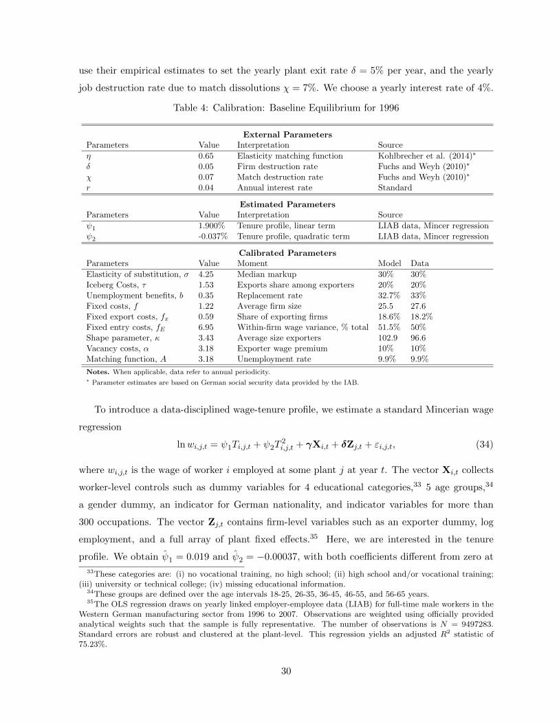
use their empirical estimates to set the yearly plant exit rate δ = 5% per year, and the yearly
job destruction rate due to match dissolutions χ = 7%. We choose a yearly interest rate of 4%.
Table 4: Calibration: Baseline Equilibrium for 1996
External ParametersParameters Value Interpretation Source
η 0.65 Elasticity matching function Kohlbrecher et al. (2014)∗
δ 0.05 Firm destruction rate Fuchs and Weyh (2010)∗
χ 0.07 Match destruction rate Fuchs and Weyh (2010)∗
r 0.04 Annual interest rate Standard
Estimated ParametersParameters Value Interpretation Source
ψ1 1.900% Tenure profile, linear term LIAB data, Mincer regressionψ2 -0.037% Tenure profile, quadratic term LIAB data, Mincer regression
Calibrated ParametersParameters Value Moment Model Data
Elasticity of substitution, σ 4.25 Median markup 30% 30%Iceberg Costs, τ 1.53 Exports share among exporters 20% 20%Unemployment benefits, b 0.35 Replacement rate 32.7% 33%Fixed costs, f 1.22 Average firm size 25.5 27.6Fixed export costs, fx 0.59 Share of exporting firms 18.6% 18.2%Fixed entry costs, fE 6.95 Within-firm wage variance, % total 51.5% 50%Shape parameter, κ 3.43 Average size exporters 102.9 96.6Vacancy costs, α 3.18 Exporter wage premium 10% 10%Matching function, A 3.18 Unemployment rate 9.9% 9.9%
Notes. When applicable, data refer to annual periodicity.∗ Parameter estimates are based on German social security data provided by the IAB.
To introduce a data-disciplined wage-tenure profile, we estimate a standard Mincerian wage
regression
lnwi,j,t = ψ1Ti,j,t + ψ2T2i,j,t + γXi,t + δZj,t + εi,j,t, (34)
where wi,j,t is the wage of worker i employed at some plant j at year t. The vector Xi,t collects
worker-level controls such as dummy variables for 4 educational categories,33 5 age groups,34
a gender dummy, an indicator for German nationality, and indicator variables for more than
300 occupations. The vector Zj,t contains firm-level variables such as an exporter dummy, log
employment, and a full array of plant fixed effects.35 Here, we are interested in the tenure
profile. We obtain ψ1 = 0.019 and ψ2 = −0.00037, with both coefficients different from zero at
33These categories are: (i) no vocational training, no high school; (ii) high school and/or vocational training;(iii) university or technical college; (iv) missing educational information.
34These groups are defined over the age intervals 18-25, 26-35, 36-45, 46-55, and 56-65 years.35The OLS regression draws on yearly linked employer-employee data (LIAB) for full-time male workers in the
Western German manufacturing sector from 1996 to 2007. Observations are weighted using officially providedanalytical weights such that the sample is fully representative. The number of observations is N = 9497283.Standard errors are robust and clustered at the plant-level. This regression yields an adjusted R2 statistic of75.23%.
30
the 0.1% level of significance. We use these coefficients to simulate the theoretical wage profiles.
To compare the empirical estimates of column (4) to those implied by our model, we create
230 samples of simulated data, each comprising 5,000 firms and about 120,000 workers. We run
regression (34) on our simulated data, and find the coefficients ψ′1 = 0.02, ψ′2 = −0.00036, both
highly significant, and almost identical to the empirical estimates.36
We calibrate the remaining nine parameters σ, τ , b;α, κ,A, f, fX , fE to match important
moments of the German economy for the year 1996. Three of them, τ , σ, b have natural counter-
parts in the data so they can be directly calibrated, each one matching a single relevant moment.
As shown in Section 2, the median markup in 1996 is 30%, which matched to firms markup in
the model allow us to calibrate the elasticity of substitution σ. Exporters’ export sales as a
share of their total sales is τ1−σ/(1 + τ1−σ) in the model.37 Thus matching the average share
of exports in total revenues of exporters of 20% observed in the data, we obtain the benchmark
τ = 1.53. For the parameter b, we use the replacement rate of 0.33 computed by the OECD.38
Setting b = 0.35, we calibrate its ratio to the average wage and set it as close as possible to 0.33.
Finally, we assume that the productivity distribution is Pareto with shape parameter κ and
normalize, without loss of generality, the expected productivity to one by setting the minimum
possible productivity zmin = (κ− 1)/κ.
We simultaneously choose the remaining parameters, υ ≡ α, κ,A, f, fX , fE so that the
numerical steady-state solution of the model matches relevant statistics. The parameters are
calibrated in order to minimize a loss function defined by the quadratic distance between the
moments in the model and the targeted statistics. We define m = [m1,....,m6] as the vector of
the empirical moments described above, and y(υ) as the vector of equilibrium model moments
generated by some vector of parameters υ. Our calibrated parameter vector is obtained solving
numerically
υ = arg minυ∈Ξ
[(y(υ)−m) ·W · (y(υ)−m)′
]where W is the weighting matrix, a diagonal matrix with the squares of the data targets on
the diagonal, Wii = 1/m2i , and zero for all other entries. We calculate the following empirical
moments from plant-level data (see the Data Appendix B for further details): (i) the average firm
size is 27.5 employees; (ii) the share of exporting firms is 18.2%; (iii) the average size of exporting
36The averaging procedure is required to deal with sampling error.37Note that the link between τ and the share of revenues realized in foreign countries is particularly straight-
forward. Since RX = (pXqX) /τ = pDqDτ1−σ = RDτ
1−σ, we have RX/ (RD +RX) = τ1−σ/(1 + τ1−σ
).
38The OECD summary measure is defined as the average of the gross unemployment benefit replacement ratesfor two earnings levels, three family situations and three durations of unemployment. For further details, seeOECD (1994), The OECD Jobs Study (chapter 8) and Martin J. (1996).
31
firms equals 96.6 employees; (iv) the difference between average wages paid by exporters to those
paid by non-exporters (the exporter wage premium) is 10.1%;39 (v) the aggregate unemployment
rate provided by the Federal Employment Agency is equal to 9.9% in 1996; (vi) the share of
total wage variance attributable to the within-firm component is about 50%.
As shown in Table 4, our model is able to replicate these moments rather well. It is worth
stressing that the original feature of our model, within-firm wage inequality generated by directed
search, accurately matches its data counterpart. The only noticeable tension is with respect to
the distribution of firm sizes, as the model slightly overestimates the average size of exporters.
This suggests that the right-tail of the model’s distribution is somewhat thicker than the one
in the data, a well known feature of the Pareto distribution (see, e.g., Head et al., 2014).
The implied parameters values are plausible. The ad valorem tariff equivalent of trade costs
(approximately 60%), is well in line with numbers discussed in Anderson and van Wincoop
(2004). The shape parameter of the Pareto distribution, κ, is close to 3.4, the value found by
Bernard et al. (2007).
5.2 Out-of-sample tests
Dynamic moments Our theory generates a positive link between worker turnover at the
establishment level and the wages of new hires. While limitations of the LIAB data set make a
direct test of this prediction impossible,40 we can still obtain tentative estimates of the role of
plant size and growth on hiring wages. Moreover, as an out of sample test, we show that the
calibrated model produces firm level wage-growth correlations consistent with these estimates.
We define as a ‘new hire’ a worker i employed at some plant j at year t who has not been
employed at that plant in year t− 1. We run a variant of the Mincer regression (5.1), but focus
on the wages of newly hired workers wi,j,t
ln wi,j,t = ι1 lnEj,t + ι2 lnEj,t−1 + γXi,t + δZj,t + εi,j,t. (35)
Ej,t is total employment at establishment j that employs worker i at date t, vectors Xi,t and Zj,t
are defined as above.41 The estimates ι1 and ι2 are to be interpreted as conditional correlations
39The exporter wage premium is estimated in Mincer regressions without controlling for firm productivityor size. It captures the average residual wage premium paid by exporters (i.e., controlling for observed workercharacteristics). Therefore, it confounds the export status effect and the productivity effect highlighted in equation(25).
40The LIAB data set reports plant employment at some reference date for each year, but does not give infor-mation on gross turnover. Moreover, the panel suffers from substantial attrition so that the number of continuingfirms available is rather low.
41The only difference is that Xi,t contains measures of worker tenure.
32
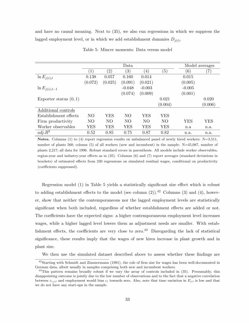
and have no causal meaning. Next to (35), we also run regressions in which we suppress the
lagged employment level, or in which we add establishment dummies Dj(i).
Table 5: Mincer moments: Data versus model
Data Model averages(1) (2) (3) (4) (5) (6) (7)
lnEj(i),t 0.138 0.057 0.160 0.014 0.015
(0.072) (0.025) (0.091) (0.021) (0.005)lnEj(i),t−1 -0.048 -0.003 -0.005
(0.074) (0.009) (0.001)Exporter status (0, 1) 0.021 0.020
(0.004) (0.006)
Additional controlsEstablishment effects NO YES NO YES YESFirm productivity NO NO NO NO NO YES YESWorker observables YES YES YES YES YES n.a n.a.
adj.R2 0.52 0.85 0.75 0.87 0.82 n.a. n.a.
Notes. Columns (1) to (4) report regression results on unbalanced panel of newly hired workers: N=3,511,
number of plants 560; column (5) of all workers (new and incumbent) in the sample: N=45,087, number of
plants 2,217; all data for 1996. Robust standard errors in parenthesis. All models include worker observables,
region-year and industry-year effects as in (35). Columns (6) and (7) report averages (standard deviations in
brackets) of estimated effects from 230 regressions on simulated residual wages, conditional on productivity
(coefficients suppressed).
Regression model (1) in Table 5 yields a statistically significant size effect which is robust
to adding establishment effects to the model (see column (2)).42 Columns (3) and (4), howev-
er, show that neither the contemporaneous nor the lagged employment levels are statistically
significant when both included, regardless of whether establishment effects are added or not.
The coefficients have the expected signs: a higher contemporaneous employment level increases
wages, while a higher lagged level lowers them as adjustment needs are smaller. With estab-
lishment effects, the coefficients are very close to zero.43 Disregarding the lack of statistical
significance, these results imply that the wages of new hires increase in plant growth and in
plant size.
We then use the simulated dataset described above to assess whether these findings are
42Starting with Schmidt and Zimmermann (1991), the role of firm size for wages has been well-documented inGerman data, albeit usually in samples comprising both new and incumbent workers.
43This pattern remains broadly robust if we vary the array of controls included in (35). Presumably, thisdisappointing outcome is jointly due to the low number of observations and to the fact that a negative correlationbetween εi,j,t and employment would bias ι1 towards zero. Also, note that time variation in Ej,t is low and thatwe do not have any start-ups in the sample.
33
consistent with our calibrated model. We regress simulated log residual wages of newly hired
workers on simulated current and lagged log employment levels (as well as on the level of
productivity, the only time-invariant establishment characteristic in our model), and report the
averages and standard deviations of the obtained coefficients in column (6). We find that both
sizes and growth rates are correlated with wage offers but the coefficients are strikingly low, with
an elasticity of 0.015% and −0.005%, respectively. In light of the limitations of our data set, it
should not be surprising that such small correlations are difficult, if not impossible, to identify
econometrically. Thus, the lack of conclusive empirical evidence does not contradict our model
since its simulation is in line with a very weak link between firm size/growth and the wages of
new hires.44 Rather, we view the high fit between the simulated averages of our model and the
coefficients obtained in actual data as an out-of-sample check of the validity of our framework.
Conditional exporter wage premium. Columns (5) and (7) report an additional out-of-
sample check. We compare the exporter status effect implied by the model with the one obtained
in the data.45 As above, we simulate 230 samples of artificial data. We use the data to regress
log residual wages on exporter status and productivity. We average across samples and find a
coefficient of the exporter dummy that is equal to 0.020. This is again very close to the coefficient
measured in the real data.
Size distribution. Figure 3 plots the cross-sectional distribution of firm employment as a
function of firm-level age and productivity. It focuses on a subset which includes the marginal
producer z∗D and the marginal exporter z∗X . Notice that the firm size distribution exhibits a
discrete jump at the productivity cutoff z∗X . By contrast, as a function of firm age, the size
distribution is continuous. In our model, from the start of their existence, highly productive
future exporters internalize that they will end up larger than non-exporters and they put on
employment accordingly, even if they do not export yet. When they have reached the critical
size (and age) of starting to export, foreign sales jump up and domestic sales fall, leaving overall
sales (and employment) constant. This avoids the counterfactual prediction of the basic Melitz
(2003) model where exporters and non-exporters are perfectly partitioned along the productiv-
ity dimension (e.g. Bernard et al., 2003). Impullitti et al. (2013) use the interaction between
sunk export costs and idiosyncratic uncertainty to explain the existence of highly productive
non-exporters. Eaton, Kortum and Kramarz (2011) introduce firm and market specific hetero-
44A proper test would require a different procedure based on data containing detailed information about grossjobs flows at the firm level, a task that we leave to further research.
45In the calibration, we have targeted the unconditional exporter wage effect.
34
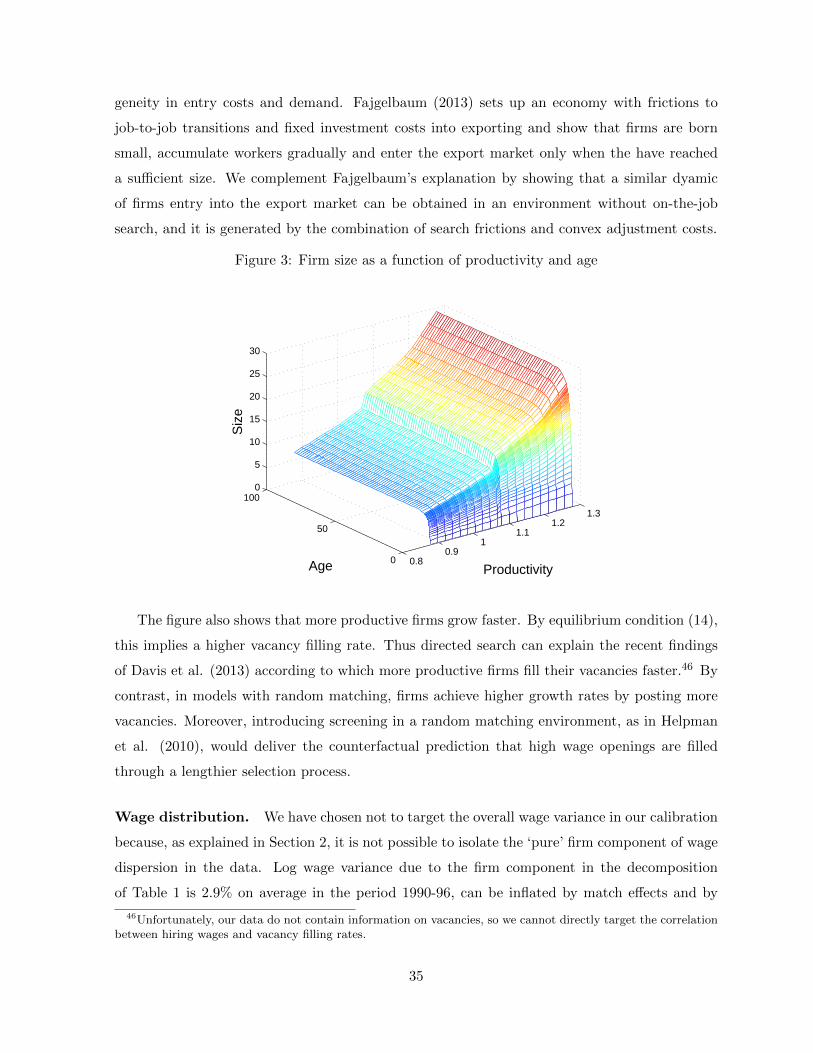
geneity in entry costs and demand. Fajgelbaum (2013) sets up an economy with frictions to
job-to-job transitions and fixed investment costs into exporting and show that firms are born
small, accumulate workers gradually and enter the export market only when the have reached
a sufficient size. We complement Fajgelbaum’s explanation by showing that a similar dyamic
of firms entry into the export market can be obtained in an environment without on-the-job
search, and it is generated by the combination of search frictions and convex adjustment costs.
Figure 3: Firm size as a function of productivity and age
0.80.9
11.1
1.21.3
0
50
1000
5
10
15
20
25
30
ProductivityAge
Siz
e
The figure also shows that more productive firms grow faster. By equilibrium condition (14),
this implies a higher vacancy filling rate. Thus directed search can explain the recent findings
of Davis et al. (2013) according to which more productive firms fill their vacancies faster.46 By
contrast, in models with random matching, firms achieve higher growth rates by posting more
vacancies. Moreover, introducing screening in a random matching environment, as in Helpman
et al. (2010), would deliver the counterfactual prediction that high wage openings are filled
through a lengthier selection process.
Wage distribution. We have chosen not to target the overall wage variance in our calibration
because, as explained in Section 2, it is not possible to isolate the ‘pure’ firm component of wage
dispersion in the data. Log wage variance due to the firm component in the decomposition
of Table 1 is 2.9% on average in the period 1990-96, can be inflated by match effects and by
46Unfortunately, our data do not contain information on vacancies, so we cannot directly target the correlationbetween hiring wages and vacancy filling rates.
35
rent sharing, as explained in Section 2. Hence, we have chosen not to target the overall wage
variance in our calibration because it is not possible to isolate the ‘pure’ firm component of wage
dispersion in the data. Nevertheless, although the pure firm effect is the only source of inequality
in our economy, the model does a good job in generating a sizable variance of log-wages of 1.25%,
thereby accounting for 43% of the residual wage dispersion attributable to firm fixed-effects in
Card et al. (2013). In Table 6 below, we report the total wage dispersion attributable to firm
fixed-effects in Card et al. (2013) for the periods 1990-96 and 2000-09 as a data reference point,
although imperfect, and compare it with the model predictions generated by the set of reforms
observed in those years.
The wages of new hires fall with firm age because younger firms grow faster, and in our
labor market with competitive search, firms foster growth by posting better compensations.
Thus workers with more seniority earn higher wages, as commonly observed in the data. Notice
that within-firm inequality cannot be obtained using random search as in, e.g., Cosar et al.
(2016). In that model, firms pay their employees equally because all wages are renegotiated at
every point in time and this firm-specific wage falls as the firm closes in to its desired size. The
importance of within-firm wage dispersion is documented by, among others, Haltiwanger et al.
(2010), Bloom et al. (2015) for US data, Mueller et al. (2015) for UK data and Helpman et al.
(2013) for Brazilian data. As can be seen in Table 2, our German data confirm the presence of
substantial pay differentials within firms.
5.3 Equilibrium properties and policy evaluation
Taking our calibration as the baseline, we evaluate whether trade, labor and product market
reforms can explain the changes in German labor market outcomes documented above. We
first feed the model the changes in parameters implied by each reform one by one, in order to
isolate their effects. We then compute the combined effect of all reforms. The objective of this
exercise is to understand and quantify the effects of the different reforms on the dynamics of
total residual wage dispersion and on its between/within-firm decomposition.
Table 6, shows the changes in the main moments between the two periods and the effects of
each reform predicted by our model. We report the key facts highlighted in Section 2. Comparing
1996 to 2009, the share of exports in total sales of exporters, the share of exporting firms in the
population, and the average size of exporters all increase, while the average size of exporters
decreases. This suggests that standard Melitz-type trade-induced selection effects have been at
work in this period.
36
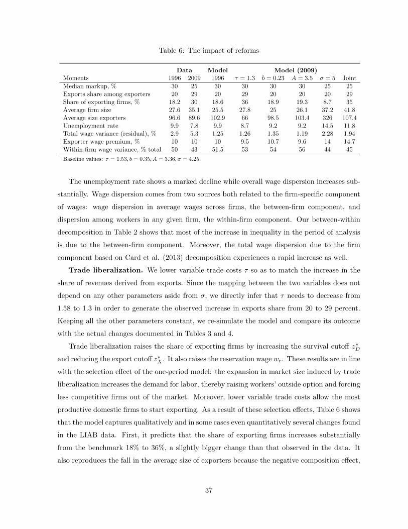
Table 6: The impact of reforms
Data Model Model (2009)Moments 1996 2009 1996 τ = 1.3 b = 0.23 A = 3.5 σ = 5 Joint
Median markup, % 30 25 30 30 30 30 25 25Exports share among exporters 20 29 20 29 20 20 20 29Share of exporting firms, % 18.2 30 18.6 36 18.9 19.3 8.7 35Average firm size 27.6 35.1 25.5 27.8 25 26.1 37.2 41.8Average size exporters 96.6 89.6 102.9 66 98.5 103.4 326 107.4Unemployment rate 9.9 7.8 9.9 8.7 9.2 9.2 14.5 11.8Total wage variance (residual), % 2.9 5.3 1.25 1.26 1.35 1.19 2.28 1.94Exporter wage premium, % 10 10 10 9.5 10.7 9.6 14 14.7Within-firm wage variance, % total 50 43 51.5 53 54 56 44 45
Baseline values: τ = 1.53, b = 0.35, A = 3.36, σ = 4.25.
The unemployment rate shows a marked decline while overall wage dispersion increases sub-
stantially. Wage dispersion comes from two sources both related to the firm-specific component
of wages: wage dispersion in average wages across firms, the between-firm component, and
dispersion among workers in any given firm, the within-firm component. Our between-within
decomposition in Table 2 shows that most of the increase in inequality in the period of analysis
is due to the between-firm component. Moreover, the total wage dispersion due to the firm
component based on Card et al. (2013) decomposition experiences a rapid increase as well.
Trade liberalization. We lower variable trade costs τ so as to match the increase in the
share of revenues derived from exports. Since the mapping between the two variables does not
depend on any other parameters aside from σ, we directly infer that τ needs to decrease from
1.58 to 1.3 in order to generate the observed increase in exports share from 20 to 29 percent.
Keeping all the other parameters constant, we re-simulate the model and compare its outcome
with the actual changes documented in Tables 3 and 4.
Trade liberalization raises the share of exporting firms by increasing the survival cutoff z∗D
and reducing the export cutoff z∗X . It also raises the reservation wage wr. These results are in line
with the selection effect of the one-period model: the expansion in market size induced by trade
liberalization increases the demand for labor, thereby raising workers’ outside option and forcing
less competitive firms out of the market. Moreover, lower variable trade costs allow the most
productive domestic firms to start exporting. As a result of these selection effects, Table 6 shows
that the model captures qualitatively and in some cases even quantitatively several changes found
in the LIAB data. First, it predicts that the share of exporting firms increases substantially
from the benchmark 18% to 36%, a slightly bigger change than that observed in the data. It
also reproduces the fall in the average size of exporters because the negative composition effect,
37
due to the decrease in the export threshold, dominates the increase in size among pre-reform
exporters. This overall gain explains why average firm size adjusts in the opposite direction.
The key result of this comparative statics is that the observed trade liberalization does not seem
to affect neither the overall level of wage inequality nor its between-within firm breakdown.
Another interesting feature of the comparative statics exercise is the prediction that em-
ployment goes up. The impact on unemployment is particularly significant since it decreases
from 9.8% to 8.7% solely because of trade liberalization, hence reproducing most of the drop in
unemployment shown in the data.47 This result, interpreted in the light of our findings in the
one-period model discussed in Section 4.4, suggest that the efficiency effect of trade liberaliza-
tion prevails. By increasing firm size, trade increases firm competition for workers, forcing them
to offer higher job finding rates for each wage offer, thereby increasing aggregate employment.
To sum-up, decreasing τ from 1.58 to 1.3 explains most of the adjustments in firm size
and export status as well as in aggregate employment. However, the degree of wage dispersion
as measured by the standard deviation of log-wages and the decomposition into between and
within-firm inequality remains almost flat. Also, the difference between the average exporter
wage and the average non-exporter wage (the exporter wage premium) does not change much,
while the data show an increase. This is not necessarily at odds with the one-period model
because the exporter wage premium confounds the productivity effect and the export status
effect in equation (25).
Hence, while reasonable changes in τ go a long way in explaining the observed reduction
in the German unemployment rate from 1996 to 2007, trade appears to be of little relevance
for the observed increase in residual wage dispersion. This suggests that other mechanisms are
at work in our dynamic framework. One plausible explanation is that firms smooth the effect
of trade-induced reallocations on wage dispersion. By contrast, in the one period model firms
adjust immediately to the new post-liberalization optimal size, and this leads to a larger jump
in the wage contract they offer.
Labor market deregulation. The first institutional change that we analyze is the reduc-
tion in unemployment benefits associated with the Hartz IV reform. The OECD estimates that
the replacement rate in Germany was reduced by about 30% from 2001 to 2009, which applied
to our benchmark benefit gives b = 0.23. Lowering b reduces the reservation wage wr as well as
the two cutoffs z∗D and z∗X . Intuitively, a reduction in benefits lowers workers’ outside option,
making survival easier for firms, allowing marginal non-exporters to enter the foreign market.
47Interestingly, this is very close to the employment gain of about 440,000 workers that Dauth et al. (2014)attribute to increased trade in their econometric work.
38
In Table 6 we report the impact that unemployment benefits have on labor market out-
comes.48 Perhaps surprisingly, b has a smaller effect than τ on unemployment, which declines
by less than three quarters of a percentage point. This is in line with the results in Launov
and Waelde (2013). They estimate an equilibrium matching model with spell-dependent unem-
ployment benefits and find that the Hartz IV reform reduced unemployment by 0.7 percentage
points. The model also predicts that residual inequality increases with smaller b: since the lower
bound of the wage distribution is pinned down by the reservation wage wr, a reduction in benefits
shifts the support of the wage distribution to the left thereby making it more dispersed. Finally,
the reduction in the unemployment rate has a counterfactual effect on the between-within firm
inequality split, increasing the share of inequality attributed to the within-firm component.
The Hartz III package of reforms focused on the Federal Employment Agency with the
objective to increase the efficiency of job search. Fahr and Sunde (2009) estimate the effects of
this reform and argue that it has increased search efficiency by between 5 and 10%. We model
this by simulating the effects of a an increase in A, from 3.36 to 3.7. Not surprisingly, increasing
matching efficiency lowers the intensity of search frictions, thereby reducing unemployment.
The effect is quantitatively strong,49 but the impact on inequality is counterfactual as better
matching efficiency reduces wage dispersion. Improvements in the matching technology relax the
trade off between wages and job filling rates. More productive firms resort less to wage incentives
in order to raise their growth rates. Hence, the reforms aimed at improving the functioning of
the public employment agency can explain part of the reduction in German unemployment but
not the increase in inequality.
Product market deregulation. The other significant change over the period of interest
relates to the ongoing process of European integration, most notably the single market program
with its ambitious reforms of product market regulation. While the single market program
presumably brought down trade costs between EU member states, it also led to deep domestic
regulatory reform within each country. Indeed, Wolfl et al. (2009) document that the OECD
index of product market regulation (PMR) intensity for Germany fell from 2 in 1998 to 1.37 in
2008, with two thirds of this change taking place by 2003. This corresponds to a 24% drop in the
PMR intensity by 2003 and a 36% by 2008. Griffith et al. (2004) and (2010) provide empirical
48The simulation of the Hartz IV reform has to be treated with caution because countries are symmetric inour model. This approximation is not too problematic for episodes of trade liberalization since they are generallyimplemented through multilateral agreements. By contrast, Germany was rather isolated in its push towardslabor market deregulation, to the extent that it has sometimes been accused of promoting beggar-thy-neighborpolicies.
49Launov and Waelde (2013) set up a random search model with heterogenous workers and show that thechange in matching efficiency implied by Hartz III explains about one third of the post-reform reduction inunemployment.
39
evidence that the deregulation reforms carried out under the EU Single Market Program in
the early 1990s increased product market competition, as measured by a reduction in average
sectorial profitability, in all major European economies. Using our firm level data we have
computed the average and median markups for Germany in the period of interest. In Figure 2
we show that the markup, computed as profits share of revenues, has a median value of 30% in
our benchmark year 1996, and it decreases to 28% in 2007 and to 25% in 2009, a trend in line
with the empirical evidence for other European countries.
Following Blanchard and Giavazzi (2003), we posit that product market reforms (encom-
passing trade liberalization) increase competition, thereby decreasing profit margins. A reduced
form way to implement this is to experiment with an increase in the elasticity of substitution.
The drop in markup observed in the data between 1996 and 2009 implies an increase in the
elasticity of substitution σ, from 4.25 to 5. Table 6 shows that, in spite of its relatively modest
size, such a change has a significant impact on the economy. In particular, it increases both
residual wage inequality and the share of inequality accounted for by the between firm channel.
Overall residual inequality increases from 1.25% to 2.28% accounting for about most of the in-
crease observed in the data where total wage variance due to the firm component increases from
2.9% in 1996 to 5.3% in 2009. Intuitively, a higher σ makes the mapping between productivity
and optimal size steeper, as can be seen from (17). This effect is due to the role of demand
elasticity in shaping the link between firms’ productivity and their optimal size. Higher demand
elasticity increases the size premium of more productive firms, thereby increasing the dispersion
of firm size. Since wage inequality in our economy is generated by dispersion in firm size, higher
product market competition increases firm-size dispersion and wage inequality. Moreover, these
adjustments imply that recruitment becomes more competitive, which intensifies search friction-
s and pushes up the rate of unemployment. Interestingly, among all reforms only the increase
in product market competition yields a decrease in the share of inequality attributable to the
within-firm component, matching most of the decline observed in the data. This result is in line
with recent findings by Bloom et al. (2015). Focusing on a new matched employer-employee da-
ta set covering all US firms in the period 1976-2012 they find that most of the observed increase
in inequality can be attributed to rising dispersion between firms in the average wage they pay.
To the best of our knowledge, our paper is the first to uncover this interesting link be-
tween demand elasticity, firm size and wage dispersion. Admittedly, the structure of our model
economy with monopolistic competition and CES preference is too simple to allow a proper
identification of which among the many reforms we consider had a major impact on product
market competition, thereby shaping the evolution of firm size dispersion and wage inequali-
40
ty. Under this market structure, firms market power cannot be affect by any change in the
institutional environment. There is substantial empirical evidence that trade liberalization has
pro-competitive effects via a reduction of markups at the setorial and firm level.50 In line with
Krugman (1979), our model could be easily extended to embed a reduced-form representation of
variable markups assuming that the elasticity of substitution is a function of firm size. Hence,
trade liberalization would have pro-competitive effects which would spread both firm size and
wage dispersion. Hence, although we cannot exclude that trade had a role in shaping the dy-
namics of inequality in Germany, a key message of our paper is that in order to fully assess
this role we must move to an economy with variable markups. Unfortunately, modeling variable
markups in open economies with firm heterogeneity and in general equilibrium is hard, even
in model with perfectly competitive labor markets. Melitz and Ottaviano (2008), offer a first
step in this direction, setting up a partial equilibrium version of the Melitz model with variable
markups obtained moving away from CES preferences. Recent contribution by Feenstra (2014)
and Demidova (2016) have tried to extend the model to a general equilibrium set up. These con-
siderations suggest that an important avenue for future research is to embed variable markups
in our economy in order to carefully identify the effects of diffent policy changes on inequality,
first among them the effect of trade liberalization.
Interactions between reforms. To take stock, trade liberalization can explain a sub-
stantial share of the adjustments in employment as well as in the cross-sectional distribution
of firms characteristics. But its effect on residual inequality is rather marginal. Given that a
similar conclusion holds for labor market reforms, the model singles out higher competition in
domestic product markets as the main force behind the increase in residual inequality. Having
determined the qualitative effects of each channel, we now assess whether their interaction can
account for the changes observed in the data.
The results of this joint experiment is summarized in the last column of Table 6. Quali-
tatively, the combined policy changes generate responses in endogenous variables which are in
line with the data, except for the unemployment rate which is predicted – counterfactually –
to increase as a consequence of fiercer product market competition. Quantitatively, the model
successfully matches about half of the changes in moments as shown in Table 6. It works best
for export shares of exporters, the average size of exporters, and the share of within-firm wage
inequality. It predicts an increase of overall inequality by about 50% (from 1.23 to 1.86%), while
the data see an increase by 83% (from 2.9 to 5.3%).
50See Feenstra and Weinstein (2016) and De Loecker, Goldberg, Khandelwal, and Pavcnik (2016) for recentcontributions.
41
6 Conclusion
We build a model where firm dynamics and directed search on the labor market produce wage
dispersion among homogenous workers. We use it to explore the effects of trade, product, and
labor market reforms on residual inequality and unemployment. A one-period version of the
model can be solved in closed form and provides an analytical characterization of the mechanisms
linking trade and inequality. It generates an inverted U-shape relationship between trade and
inequality which hinges on the presence of an export wage premium: trade liberalization increases
inequality when trade costs are high and few firms pay the premium, but it reduces it when trade
costs are low and most firms pay the premium. The effect of trade on jobs is also ambiguous
and strictly dependent on the shape of adjustment costs.
We use German matched employer-employees data to calibrate the dynamic model and ex-
plore its properties numerically. Going beyond trade, we also study the roles of labor and
product market reforms. The main mechanisms linking trade and labor market outcomes high-
lighted in the one-period model continue to provide intuition. Moreover, the interaction between
wage posting and firm growth explains important firm-level regularities recently highlighted in
the empirical literature. First, firms increase their rate of growth by posting higher wages and
filling their vacancies faster. Second, productivity distributions of exporters and non-exporters
show partial overlap. Third, wage dispersion occurs both between and within firms.
Matching key statistics allows us to use the model for a quantitative assessment of the
impact of trade and institutional reforms on the German labor market. Focusing on the period
1996-2007 we find that neither the massive increase in German trade openness, nor the main
features of the Hartz labor market reforms, can explain the sharp increase in residual wage
dispersion observed in the data. By contrast, higher competition in the product market, nested
into the model as an increase in demand elasticity, has a strong effect on inequality, potentially
accounting for the whole increase in German wage dispersion. Finally, lower trade costs can
account for a sizable fraction of the decline in unemployment observed in the data, in contrast
to a general increase in product market competition which turns out to drive up unemployment.
Our analysis suggests several directions for future research. One possible extension would
analyze more deeply the role of smooth firm growth in shaping the trade-inequality nexus, by
comparing dynamic models to their static counterparts. Secondly, since our results suggest that
wage dispersion is highly responsive to changes in demand elasticity, introducing endogenous
markups could potentially strengthen the quantitative link between trade and inequality.
42
References
Acemoglu, Daron, and Robert Shimer, 1999, “Holdups and Efficiency with Search Frictions”,
International Economic Review 40: 827–928.
Acemoglu, Daron, 2003, “Patterns of Skill Premia”, Review of Economic Studies 70(2): 199-230.
Amiti, Mary, and Donald Davis, 2011, “Trade, Firms, and Wages: Theory and Evidence”,
Review of Economic Studies 79: 1-36.
Autor, David, David Dorn, and Gordon Hanson (2013).“The China Syndrome: Local Labor
Market Effects of Import Competition in the United States”, American Economic Review 103(6):
2121-2168.
Autor, David, David Dorn, Gordon Hanson, and Jae Song (2014). “Trade Adjustment: Worker
Level Evidence”, Quarterly Journal of Economics 129(4): 1799-1860.
Baumgarten, Daniel, 2013, “Exporters and the Rise in Wage Inequality: Evidence from German
Linked Employer-Employee Data”, Journal of International Economics 90(1): 201-217.
Barth, Erling, Alex Bryson, James C. Davis, Richard Freeman, 2014, “It’s Where You Work:
Increases in Earnings Dispersion across Establishments and Individuals in the U.S.”, NBER
Working Paper No. 20447.
Bellon, Matthieu, 2016, “Trade liberalization and inequality: a dynamic model with firm and
worker heterogeneity”, Columbia University Working Paper.
Bernard, Andrew, Bradford Jensen, Jonathan Eaton, and Samuel Kortum, 2003, “Plants and
Productivity in International Trade”, American Economic Review 93(4): 1268-290.
Bernard, Andrew, Stephen Redding, and Peter Schott, 2007, “Comparative advantage and het-
erogeneous firms”, Review of Economic Studies 74(1): 31–66.
Blanchard, Olivier, and Francesco Giavazzi, 2003, “Macroeconomic Effects of Regulation and
Deregulation in Goods and Labor Markets”, Quarterly Journal of Economics 118(3): 897-907.
Bloom, Nicholas, Fatih Guvenen, David Price, and Jae Song (2015), “Firming up Inequality,”
mimeo Stanford.
Blundell, Richard, and Ben Etheridge, 2010, “Consumption, Income and Earnings Inequality in
Britain”, Review of Economic Dynamics 13(1): 76–102.
43
Card, David, Joerg Heining, and Patrick Kline, 2013, “Workplace Heterogeneity and the Rise
of West German Wage Inequality”, Quarterly Journal of Economics 128(3): 967-1015.
Cosar, Kerem, Nezih Guner, and James Tybout, 2016, “Firm Dynamics, Job Turnover, and
Wage Distributions in an Open Economy”, American Economic Review, 106(3): 625-63.
Dauth, Wolfgang, Sebastian Findeisen, and Jens Suedekum, 2014, “The Rise of the East and the
Far East: German Labor Markets and Trade Integration ”, Journal of the European Economic
Association 12(6): 164-1675.
Davis, Donald, and James Harrigan, 2011, “Good Jobs, Bad Jobs, and Trade Liberalization”,
Journal of International Economic 84: 26-36.
Davis, Stephen, Jason Faberman, and John Haltiwanger, 2013, “The Establishment-Level Be-
havior of Vacancies and Hiring”, Quarterly Journal of Economics 128 (2): 581-622.
De Loecker, Jan, Penny Goldberg, Amit Khandelwal, and Nina Pavcnik, 2016. “Prices, Markups
and Trade Reform”, Econometrica, forthcoming.
Demidova, Svetlana, 2016, “Trade Policies, Firm Heterogeneity, and Variable Markups”, mimeo.
Dustmann, Christian, Johannes Ludsteck, and Ute Schoenberg, 2009, “Revisiting the German
Wage Structure”, Quarterly Journal of Economics 124(2): 843–881.
Egger, Hartmut, and Udo Kreickemeier, 2009, “Firm Heterogeneity and the Labor Market Ef-
fects of Trade Liberalization”, International Economic Review 50: 187–216.
Egger, Hartmut, Peter Egger, and Udo Kreickemeier, 2013, “Trade, Wages, and Profits”, Euro-
pean Economic Review 64: 332–350.
Eaton, Jonathan, Sam Kortum, and Francis Kramarz, 2011, “An Anatomy of International
Trade: Evidence From French Firms”, Econometrica, Vol. 79, No. 5, pp. 1453-1498.
Epifani, Paolo, and Gino Gancia, 2008. ”The Skill Bias of World Trade,” Economic Journal
118(530): 927-960.
Fahr, Rene, and Uwe Sunde, 2009, “Did the Hartz Reforms Speed Up Job the Matching Process?
A Macroeconomic Evaluation Using Empirical Matching Functions”, German Economic Review
10(3): 284-316.
44
Fajgelbaum, Pablo, 2013, “Labor Market Frictions, Firm Growth, and International Trade”,
NBER Working Paper 19492.
Feenstra, Robert, and David Weinstein, 2016. “Globalization, Competition, and U.S. Welfare,
joint with David Weinstein”, forthcoming, Journal of Political Economy.
Feenstra, Robert, 2014. “Restoring the Product Variety and Pro-competitive Gains from Trade
with Heterogeneous Firms and Bounded Productivity”, NBER Working Paper No. 19833.
Felbermayr, Gabriel, Julien Prat, and Hans-Jorg Schmerer, 2011, “Globalization and labor mar-
ket outcomes: Wage bargaining, search frictions, and firm heterogeneity”, Journal of Economic
Theory 146: 39–73.
Fuchs, Michaela, and Antje Weyh, 2010, “The Determinants of Job-Creation and Destruction:
Plant-Level Evidence for Eastern and Western Germany”, Empirica 111: 765–788.
Fuchs-Schuendeln, Nicole, Dirk Krueger, and Mathias Sommer, 2010, “Inequality Trends for
Germany in the Last Two Decades: A Tale of Two Countries“, Review of Economic Dynamics
13: 103–132.
Garibaldi, Pietro, and Espen Moen, 2010, “Job to Job Movements in a Simple Search Model”,
American Economic Review 100(2): 343–47.
Hall, Robert, and Alan Krueger, 2012, “Evidence on the Incidence of Wage Posting, Wage
Bargaining, and on-the-Job Search”, American Economic Journal: Macroeconomics 4(4): 56-
67.
Harrigan, James, and Ariell Reshef, 2012, “Skill Biased Heterogeneous Firms, Trade Liberaliza-
tion and the Skill Premium”, Canadian Journal of Economics, forthcoming.
Hauptmann, Andreas, and Hans-Jorg Scherer, 2013. “Do Exporters Pay Fair-Wage Premiums”,
Economics Letters 121: 179-182.
Head, Keith, Thierry Mayer, and Matthias Thoenig, 2014, “Welfare and Trade Without Pareto”,
American Economic Review Papers and Proceedings, 104(5): 310-316.
Heathcote, Johnathan, Fabrizio Perri, and Giovanni Violante, 2010, “Unequal We Stand: An
Empirical Analysis of Economic Inequality in the United States”, Review of Economic Dynamics
13(1): 15–54.
45
Helpman, Elhanan, Oleg Itskhoki, Marc-Andreas Muendler, and Stephen Redding, 2012, “In-
equality and Unemployment in a Global Economy”, NBER Working Paper No. 17991.
Helpman, Elhanan, and Oleg Itskhoki, 2010, “Labor Market Rigidities, Trade and Unemploy-
ment”, Review of Economic Studies 77(3): 1100-1137.
Helpman, Elhanan, Oleg Itskhoki, and Stephen Redding, 2010, “Inequality and Unemployment
in a Global Economy”, Econometrica 78(4): 1239-1283.
Hertweck, Matthias, and Oliver Sigrist, 2012, “The Aggregate Effects of the Hartz Reforms in
Germany”, Working Paper 2012-38, University of Konstanz.
Hornstein, Andreas, Per Krusell, and Gianluca Violante, 2011, “Frictional Wage Dispersion in
Search Models: A Quantitative Assessment ”, American Economic Review 101(7): 2873-2898.
Impullitti, Giammario, Alfonso Irarrazabal, and Luca David Opromolla, 2013, “A Theory of
Entry into and Exit from Exports Markets”, Journal of International Economics 90(1): 75-90.
Jacobi, Lena & Kluve, Jochen, 2007. “Before and after the Hartz reforms: The performance of
active labour market policy in Germany”, Zeitschrift fur ArbeitsmarktForschung - Journal for
Labour Market Research 40(1): 45-64.
Jappelli, Tullio, and Luigi Pistaferri, 2010, “Does Consumption Inequality Track Income In-
equality in Italy?”, Review of Economic Dynamics 13(1): 133–153.
Kaas, Leo and Philipp Kircher, 2015, “Efficient Firm Dynamics in a Frictional Labor Market”,
American Economic Review 105(10):3030-60.
Krebs, Tom, and Martin Scheffel, 2013, “Macroeconomic Evaluation of Labor Market Reform
in Germany”, mimeo.
Kohlbrecher, Britta, Christian Merkl, and Daniela Nordmeyer, 2013, “The Matching Function:
A Selection-Based Interpretation”, LASER Discussion Papers - Paper No. 70.
Koske, Isabell, Isabelle Wanner, Rosa Bitette, Omar Barbiero, 2015, “The 2013 update of the
OECD’s database on product market regulation: Policy insights for OECD and non-OECD
countries”, OECD Economics Department Working Papers, No. 1200.
Launov, Andrei, and Klaus Waelde, 2013, “Estimating Incentive and Welfare Effects of Non-
Stationary Unemployment Benefits”, International Economic Review 54(4): 1159–1198.
46
Manning, Alan, 2006, “A generalised model of monopsony”, Economic Journal 116: 84-100.
Martin J., 1996, “Measures of Replacement Rates for the Purpose of International Comparisons:
A Note”, OECD Economic Studies, No, 26.
Menzio, Guido, and Shouyong Shi, 2010, “Block Recursive Equilibria for Stochastic Models of
Search on the Job”, Journal of Economic Theory 145 (4): 1453-1494.
Merz, Monika, and Eran Yashiv, 2007, “Labor and the Market Value of the Firm”, American
Economic Review 97: 1419-1431.
Moen, Espen, 1997, “Competitive Search Equilibrium”, Journal of Political Economy 105(2):
385–411.
Mueller, Holger, Paige P. Ouimet, Elena Simintzi, 2015, “Wage Inequality and Firm Growth”,
NBER Working Paper No. 20876.
OECD, 2011, “Divided We Stand: Why Inequality Keeps Rising”, OECD Publishing, Paris.
Roberts, Mark, and James Tybout, 1997, What Makes Exports Boom?, in Directions in Devel-
opment Series, The World Bank, 1997.
Shimer, Robert, 2010, Labor Markets and Business Cycle,. Princeton University Press.
Torres, Sonia, Pedro Portugal, John Addison, and Paulo Guimaraes, 2013, “The Sources of Wage
Variation: A Three-Way High-Dimensional Fixed Effects Regression Model”, IZA Discussion
Paper 7276.
Wolfl, Anita, Isabelle Wanner, Tomasz Kozluk, and Giuseppe Nicoletti, 2009, “Ten years of
product market reform in OECD countries - insights from a revised PMR indicator”, OECD
Economics Department Working Paper No. 695.
Woodcock, Simon, 2008, “Wage Differentials in the Presence of Unobserved Worker, Firm, and
Match Heterogeneity”, Labour Economics 15(4): 771-793.
Xing, Chunbing, and Shi Li, 2012, “Residual wage inequality in urban China, 1995–2007”, China
Economic Review 23(2): 205–222.
Yeaple, Stephen, 2005, “A Simple Model of Firm Heterogeneity, International Trade, and
Wages”, Journal of International Economics, 65(1): 1-20.
47

A Proofs
A.1 Proof of Proposition 2
The only dynamic component of the optimality conditions is ∂Ψ (`a, I) /∂`a. Directly differentiating itsexpression in (11) yields
(r + δ + χ)∂Ψ (`a, `; z)
∂`a= R1 (`a, I; z) +
∂2Ψ (`a, I; z)∂`2a
[q(θa)va − χ`a] ,
where we add the number of the independent variable as a subscript to denote its partial derivative. Theexpression above makes clear that ∂Ψ (`a, I) /∂`a is the shadow value of labor since it is equal to thediscounted sum of marginal output. The term on the right hand side can be expressed as51
∂2Ψ (`a, I; z)∂`2a
[q(θa)va − χ`a] =∂2Ψ (`a, I; z)
∂`2a˙a =
d
da
(∂Ψ (`a, I; z)
∂`a
)=
d
da
(C ′ (va)
q(θa)+
w (θa)
r + δ + χ
)=C ′′ (va) vaq(θa)− C ′ (va) q′(θa)θa
q(θa)2+w′ (θa) θar + δ + χ
.
Reinserting this equality into the previous equation, we obtain
(r + δ + χ)
[C ′ (va)
q(θa)+
w (θa)
r + δ + χ
]− C
′′ (va) vaq(θa)− C ′ (va) q′(θa)θaq(θa)2
− w′ (θa) θa
r + δ + χ= R1 (`a, I; z) . (36)
The dynamics condition is too intricate to be analyzed at this level of generality. This is why we imposethe additional Assumptions A1 and A2. When recruitment costs are isoelastic, i.e., C (v) = vα, (14) isequivalent to vα−1
a = (1− η) ρ/ (ηαθa) and the dynamic equation (36) reads
(r + δ + χ)αvα−1
a
q(θa)+ w (θa)− α(α− 1)vα−2
a vaq(θa)− αvα−1a q′(θa)θa
q(θa)2− w′ (θa) θar + δ + χ
= R1 (`a, I; z) . (37)
Assumption A2 allows us to simplify this equation further by expressing analytically the slope va of thevacancy schedule with respect to age. When the matching function is Cobb-Douglas, i.e., q(θ) = Aθ−η,
va = − θaθ− αα−1
a
α− 1
[(1
η− 1
)ρ
α
] 1α−1
,
and so
αvα−1a
q(θa)
[r + δ + χ− (α− 1)
vava
+q′(θa)θaq(θa)
]=
(1
η− 1
)ρ
θaq(θa)
[r + δ + χ+
θaθa
(1− η)
]. (38)
Reinserting (38) into (37) and substituting out w′ (θa), we finally obtain
1
θaq(θa)
(r + δ + χ+
θaθa
(1− η)
)=η
ρ[R1 (`a, I; z)− wr] . (39)
In order to solve this equation, we use the following change of variable ϑa , [θaq(θa)]−1
= A−1θη−1a so
that
ϑa = (η − 1)A−1θη−2a θa =
1
θaq(θa)
θaθa
(η − 1) .
51The third equality follows from (12) .
48

Thus (39) is equivalent to
ϑa (r + δ + χ)− ϑa =η
ρ[R1 (`a, I; z)− wr] . (40)
We wish to express (40) as an ODE in `a only. Straightforward algebra yields
˙a + χ`a = q(θa)va = q(θa)
[1
θa
(1
η− 1
)ρ
α
] 1α−1
= ϑη+1/(α−1)
1−ηa A1+
η+1/(α−1)1−η
[(1
η− 1
)ρ
α
] 1α−1
︸ ︷︷ ︸,ξ0
. (41)
In order to obtain ϑa, we differentiate this expression with respect to time
ϑa =1− η
η + 1/ (α− 1)
(˙a + χ`aξ0
) 1−ηη+1/(α−1) ¨
a + χ ˙a
˙a + χ`a
,
and replace it into (40) to finally derive the law of motion (16) for employment. It obeys a highly nonlinear second ODE. The employment profile of any given firm can therefore be pinned down using astarting and terminal conditions. First, given that startups have no labor force, we can set `0 = 0.52 Thesecond condition ensures that employment converges smoothly to its optimal value in the long run, sothat both ˙
a and ¨a approach zero as time goes to infinity. Eliminating ˙
a and ¨a from (16), we find that
the asymptotic level of employment ¯(z) , lima→∞ `a(z) is given by the unique solution to (17). Finallythe smooth-pasting condition ensures that the labor force schedule is everywhere differentiable, includingthe employment level `X (z) at which domestic firms start exporting. If the smooth-pasting conditionwere violated, there would be a kink at `X (z). But this cannot be optimal because adjustment costs areconvex, implying that firms could save on recruitment costs by smoothing their convergence path.53
A.2 Derivation of equation (25)
Lemma 1 For a given value of search W and average productivity z, the equilibrium locus θ (z) reads
θ (z) =
(σ
σ − 1
W
Aη
) 11−η
z−1
1−ηβσ−1 zζ
σ−1σ
[1 + I (z) τ1−σ] ζσ , (42)
where β > 0 and ζ < 0 are combinations of parameters defined in (49) and (48) .
Equation (5) implies that marginal revenue are proportional to the domestic price which, combinedwith our normalization, yields
R1 (`, I; z) =σ − 1
σpD (z) z =
σ − 1
σz . (43)
Using this identity and the functional forms in Assumptions 1 and 2, one can use the first-order conditionR1 (`, I; z) q′ (θ) = −W/θ2 to solve for the tightness associated to z
θ =
(σ
σ − 1
W
Aηz
) 11−η
. (44)
52When the revenues function R (`a, I) is isoelastic, as in Melitz’s (2003) model, marginal revenues diverge toinfinity as ` goes to zero. This implies that the ODE (16) admits a singularity at ` = 0. Yet it is well behaved forany arbitrarily small initial size. Hence, in the simulation, we follow Garibaldi and Moen (2010) and circumventthis technical difficulty by assuming that `0 = ε. Letting ε go to zero illustrates that, for sufficiently small εs, theoptimal recruitment schedule is not significantly affected by the choice of ε
53Smooth-pasting is a standard optimality condition in firm entry models, explored in details in Dixit andPindyck (1994) and applied to entry into and exit from the export market in Impullitti, et al. (2013).
49

Similarly, reinserting our functional forms into equation (24), one obtains a closed form solution for v asa function of θ
v (z) =
(1− ηηα
W
θ (z)
) 1α−1
. (45)
We now explain how posted wages can be derived for all productivity levels. First, note that marginalrevenues are related in the following fashion
R1 (`, I; z)
R1
(˜, 0; z
) =(zz
)σ−1σ [
1 + I (z) τ1−σ]1/σ ( ˜
` (z)
)1/σ
=
(θ
θ (z)
)1−η
. (46)
The second equality results from the first order condition R1 (`, I; z) q′ (θ) = −W/θ2, which–under ourparametric assumptions–simplifies to R1 (`, I; z) = W/
(ηAθ1−η). Since ` = q (θ) v, one can solve for the
employment levels using equation (45) and substitute them out of equation (46) to obtain
z
z=[1 + I (z) τ1−σ] 1
1−σ
(θ (z)
θ
)ζ−1 σσ−1
, (47)
where
ζ−1 , −[1− η +
1
σ
(1
α− 1+ η
)]< 0 . (48)
Tightness is inversely related to productivity as the exponent on the right-hand side of (47) is unambigu-ously negative. Observe also that the relationship depends on the export status of the firm. If a firmwith productivity z decides to export, the indicator function I (z) switches from zero to one which lowersθ (z) . As expected, everything else equal, the decision to sell on the foreign market leads to an increasein optimal employment. And, to accommodate its expansion, the firm decide to post a higher wage.
The equilibrium tightness is obtained plugging (44) into (47), with
β , −ζ σ − 1
σ
α
α− 1> 0 . (49)
The exponents of both z and z in (42) are negative. To derive the exponent of z, one replaces (44) into(47) . This yields the expression in (42) but with the following exponent for z
−(
1
1− η+ ζ
σ − 1
σ
)= − 1
1− η
[1 + ζ
σ − 1
σ(1− η)
]= − 1
1− η
[−ζ 1
σ
α
α− 1
].
Replacing the definitions of ζ and of β into the expression above yields the exponent of z and z in (42).Since the exponent of z in (42) is negative, firms with a higher productivity recruit in tighter markets(lower θ) and post higher wages. Furthermore, more productive firms post more vacancies and employmore workers in equilibrium. A higher productivity of the representative firm (z) shifts the θ (z) locusup, thereby leading to higher wages for all z.
Finally, replacing the results of the Lemma into (22) and taking logarithms,54 we obtain the wageprofile (25).
A.3 Derivation of equation (26)
Equation (26) is a direct consequence of the Lemma below.
Lemma 2 (Profits) For given aggregates W and z, operating profits are log-linear in z as
π (z;W ) + f + I (z) fX = KW−η
1−η ( αα−1 )zγzβ
[1 + I (z) τ1−σ] β
σ−1 , (50)
54We have made use of 1 + ζ [(σ − 1) /σ] (1− η) = β/ (σ − 1) .
50

where the constants K > 0 and γ > 0 are defined in (58) and (57). The productivity z of the representativefirm is given by
z =
[1
1 + %
∫ ∞z∗D
zβ[1 + I(z)τ1−σ] β
σ−1 µ (z) dz
] 1β
. (51)
The expression for z follows from the normalization of the aggregate price index P = 1. Recognizingthat pX (z) = τ1−σpD (z) and that the mass of domestically available varieties M is related to the massof domestically produced varieties MD by M = MD + %MD, since %MD measures the mass of importedvarieties, we obtain
P =
[1
M
∫ω∈Ω
p (ω)1−σ
dω
] 11−σ
=
[MD
M
∫ ∞z∗D
pD (z)1−σ [
1 + I(z)τ1−σ]µ (z) dz
] 11−σ
=
[1
1 + %
∫ ∞z∗D
pD (z)1−σ [
1 + I(z)τ1−σ]µ (z) dz
] 11−σ
.
The normalization P = 1 implies that
1 + % =
∫ ∞z∗D
pD (z)1−σ [
1 + I(z)τ1−σ]µ (z) dz . (52)
We use (46) to substitute domestic prices out as
R1 (`, I (z) ; z)
R1
(˜, 0; z
) =pD (z) z
z=
(θ
θ
)1−η
,
from which one can make use of equation (47) to express the distribution of producer prices as a functionof z
pD (z) =z
z
(θ
θ
)1−η
=
(z
z
)1+ζ σ−1σ (1−η) [
1 + I (z) τ1−σ]− ζσ (1−η). (53)
Let λ = ζ [(σ − 1) /σ] (1− η) + 1, we now show that λ = β/ (σ − 1) . Using the definition of ζ, note that
λ =α
(α− 1)σ[
1σ
(1
α−1 + η)
+ σ (1− η)] = − ζ
σ
α
α− 1=
β
σ − 1
Replacing the exponent of z/z in (53) with λ = β/ (σ − 1) and plugging the price equation into (52), weobtain (28).
In order to establish the proportionality of profits, we exploit the fact that demand functions are
such that R (z) =[1 + I (z) τ1−σ]RD (z) as well as RD (z) = (z`/z`)
(σ−1)/σRD (z) . Replacing theses
two equalities into (23) we obtain
π (z;W ) =[1 + I (z) τ1−σ] [z`D (z)
z`D (z)
]σ−1σ
z`D (z)− v (z)
θ (z)W − v (z)
α − f − I (z) fX , (54)
51

where we have suppressed the dependence of I, `D, v and θ on W and z to avoid notational clutter. UsingLemma 1, it is possible to simplify each components of π (z;W ). Starting with revenues, we observe that
z`D (z)
z`D (z)=
z
z
(1
1 + I(z)τ1−σ
)` (z)
` (z)=z
z
(1
1 + I(z)τ1−σ
)(θ
θ
) 11−α−η
=(zz
)1+ζ σ−1σ [ 1
1−α−η](
1
1 + I(z)τ1−σ
)1−ζ 1σ [ 1
1−α−η].
while
zlD (z) = zAθ1
1−α−η(
1− ηcαη
W
) 1α−1
= z1+ 1η−1 ( 1
1−α−η)W−η
1−ηαα−1K1 ,
where
K1 ,
(1
η
)− η1−η
αα−1
(σ
A (σ − 1)
) 11−η ( 1
1−α−η)A
(1− ηα
) 1α−1
. (55)
We can therefore rewrite revenues as
(1 + I(z)τ1−σ) [z`D (z)
z`D (z)
]σ−1σ
zlD (z) = K1W− η
1−ηαα−1 zγzβ
[1 + I(z)τ1−σ] β
σ−1 ,
where
β =σ − 1
σζ
α
1− α=
(σ − 1
σ
)2
ζ
(1
1− α− η)
+σ − 1
σ> 0 . (56)
The sign of β follows from ζ < 0 and α > 1. The exponent of z is
γ ,
(1
α− 1+ η
)[1
1− η+
(σ − 1
σ
)2
ζ
]+
1
σ=
α
α− 1
1
1− η− β > 0 . (57)
The last equality holds because ((σ − 1) /σ) ζ (1/ (1− α)− η) + 1 = (σ/ (σ − 1))β. To see that γ ispositive, observe that this holds true if (σ/ (σ − 1)) (1/ (1− η)) + ζ > 0. Replacing the definition of ζgiven in (48) and imposing α > 1 shows that the last inequality is indeed satisfied. Focusing now on thewage bill, we obtain
v (z)
θ (z)=
(1− ηαη
W
) 1α−1
θ (z)α
1−α =
(1− ηαη
W
) 1α−1
[(zz
(1 + I(z)τ1−σ) 1
σ−1
)ζ σ−1σ
θ
] α1−α
=
(1− ηαη
W
) 1α−1
zγzβ(1 + I(z)τ1−σ) β
σ−1 .
Finally, turning our attention to the expression for recruitment costs, we find that
v (z)α
=
(1− ηcαη
W
) αα−1
θ (z)α
1−α=
(1− ηcαη
W
) αα−1
θ
α1−α (z
z
)ζ σ−1σ
α1−α (
1 + I(z)τ1−σ)ζ 1σ
α1−α .
Hence, adding all the terms above yields
π (z; z,W ) = KW−η
1−η ( αα−1 )zγzβ
[1 + I (z;W, z) τ1−σ] β
σ−1 − f − I (z;W, z) fX .
The constant K reads
K , K1 −
[(1− ηαη
) 1α−1
+
(1− ηαη
) αα−1
](Aη
σ − 1
σ
)− 11−η
α1−α
, (58)
52

where K1 is defined in equation (55) .
A.4 Derivation of the free entry condition (30)
The free entry condition ensures that entry occurs until expected profits are exactly identical to the entrycosts fE , hence
E [π (z)] =fE
1−G (z∗D). (59)
The expectation operator E [·] aggregates over levels of z that are consistent with positive profits, i.e.,
E [π (z)] =
∫∞z∗Dπ (z) dG(z)
1−G(z∗D)=
∫ ∞z∗D
π (z)µ(z)dz . (60)
In order to use condition (59), we need to relate expected profits E [π (z)] to the profits π of the repre-sentative firm. The definition in (60) and the proportionality of profits established in Lemma 2 ensurethat
E [π (z)] + f + %fX = [π + f ]
∫ ∞z∗D
(zz
)β [1 + I(z)τ1−σ] β
σ−1 µ(z)dz.
But we know from the definition of z in (28) that the integral on the right hand side is equal to 1 + %,which implies in turn that
E [π (z)] + f + %fX = [π + f ] (1 + %) . (61)
Equation (61) provides us with the desired mapping between expected profits E [π (z)] and π. Accordingly,we can substitute π out of (59) to obtain the free entry condition
(FE) : π =1
1 + %
[fE
1−G (z∗D)+ % (fX − f)
]. (62)
Using the definition of %, expression (30) follows.
A.5 Proof of Proposition 3
Derivative of z with respect to z∗D. Denote ∂z∗X/∂z∗D ≡ k, where we know k > 1 from (29). We
rewrite expression (28) as
zβ =1
2−G (z∗D)−G (z∗X)
∫ ∞z∗D
zβ[1 + I(z)τ1−σ]β/(σ−1)
g (z) dz
∂zβ
∂z∗D=
g (z∗D) + g (z∗X) k
[2−G (z∗D)−G (z∗X)]2
∫ ∞z∗D
zβ[1 + I(z)τ1−σ]β/(σ−1)
g (z) dz
− 1
2−G (z∗D)−G (z∗X)z∗βD g (z∗D)
∂zβ
∂z∗D
z∗Dzβ
=g (z∗D) z∗D
2−G (z∗D)−G (z∗X)
[1 +
g (z∗X)
g (z∗D)k −
(z∗Dz
)β]
' G (z∗D)
2−G (z∗D)−G (z∗X)
[1 +
g (z∗X)
g (z∗D)k −
(z∗Dz
)β]∂zβ
∂z∗D
z∗Dzβ
> 0⇐⇒(
1 +g (z∗X)
g (z∗D)k
)(z
z∗D
)β> 1
which is always true since the representative firm has higher productivity than the marginal producer,
z > z∗D, and∂z∗X∂z∗D
> 1. For the same initial z∗D, an increase of z∗D has a stronger effect on z in our model
53

than in the Melitz model (where β is replaced by σ − 1).Also note that
∂zβ
∂τ
τ
zβ= −β τ1−σ
1 + τ1−σ ⇐⇒∂z
∂τ
τ
z= − τ1−σ
1 + τ1−σ .
Slope of free entry condition. We have
∂π
∂z∗D=−g (z∗X) (fX − f) k [2−G (z∗D)−G (z∗X)] + [fE + [1−G (z∗X)] (fX − f)] [g (z∗D) + g (z∗X) k]
[2−G (z∗D)−G (z∗X)]2 .
Then, ∂π/∂z∗D > 0 is equivalent to
[fE + [1−G (z∗X)] (fX − f)] [g (z∗D) + g (z∗X) k] > g (z∗X) (fX − f) k [2−G (z∗D)−G (z∗X)] ,
orπ
[(fX − f)− π]>g (z∗X)
g (z∗D)k.
Using the expression for π from (30), one can show that, under the sufficient condition fX < fE ,
(fX − f)− π = (fX − f)− fE + [1−G (z∗X)] (fX − f)
2−G (z∗D)−G (z∗X)< 0
⇐⇒ fX <fE + [1−G (z∗X)] (fX − f)
2−G (z∗D)−G (z∗X)+ f =
fE + [1−G (z∗X)] fX + [1−G (z∗D)] f
2−G (z∗D)−G (z∗X).
The condition is equivalent to
fX <fE
1−G (z∗D)+ f ,
which always holds if fX < fE . Moreover,
∂π
∂z∗D
z∗Dπ
∣∣∣∣FE
=[g (z∗D) + g (kz∗D) k] z∗D2−G (z∗D)−G (z∗X)
.
Slope of zero cutoff profit condition. The ZCP is identical to the one derived by Melitz (2003)for the case of a closed economy. Totally differentiating with respect to z∗D, one obtains
∂π
∂z∗D
z∗Dπ
∣∣∣∣ZPC
= − β
1− (z∗D/z)β
(1− ∂z
∂z∗D
z∗Dz
)= − 1
1− (z∗D/z)β
(β − g (z∗D) z∗D
2−G (z∗D)−G (z∗X)
[1− (z∗D/z)
β+g (z∗X) k
g (z∗D)
]).
Melitz (2003) shows that for standard families of distribution functions, this expression is non-positive.For given z∗D, we obtain
∂π
∂z
z
π
∣∣∣∣ZPC
=β
1− (z∗D/z)β,
which is positive when β > 1 since 1− (z∗D/z)β> 0. In terms of fundamental parameters, the restriction
β > 1 is met if σ > 1 + α. To see this, we employ the definition of β
β =(σ − 1)α
(α− 1) [(1− η)σ + η] + 1.
It is easy to show that β > 1 ⇐⇒ [1 + η (α− 1)] (σ − 1) > α. Since 1 + η (α− 1) > 1, we have σ >1 + α =⇒ β > 1.
54

A.6 Derivation of equation (33)
The aggregate level of employment is by definition equal to
L = MD
∫ ∞z∗D
` (z)µ (z) dz = MDA
(1− ηαη
W
) 1α−1
∫ ∞z∗D
θ (z)−(η+ 1
α−1 ) µ (z) dz . (63)
To simplify this expression, we have to derive the mass of domestic firms MD. Given that a firm with pro-ductivity z recruits his workers from a pool of unemployed workers with mass s (z) = ` (z) / [θ (z) q (θ (z))],integrating over all levels of productivity yields
S = MD
∫ ∞z∗D
[` (z)
θ (z) q (θ (z))
]µ (z) dz = MD
(1− ηαη
W
) 1α−1
∫ ∞z∗D
θ (z)α
1−α µ (z) dz , (64)
where S is the mass of job seekers. Lemma 1 allows us to simplify the integral∫ ∞z∗D
θ (z)α
1−α dµ (z) =
∫ ∞z∗D
[θ(zz
)ζ σ−1σ [
1 + I (z) τ1−σ] ζσ ] α1−α
µ (z) dz
= θα
1−α
∫ ∞z∗D
(zz
)β [1 + I (z) τ1−σ] β
σ−1 µ (z) dz .
But we know from (28) that the integral on the right hand side equals 1 + %, which implies in turn that∫ ∞z∗D
θ (z)α
1−α µ (z) dz = θα
1−α (1 + %) .
Reinserting this equality into (64) and setting S = 1, we find that
MD =
(1− ηαη
W
) 11−α θ
αα−1
1 + %.
Substituting MD in (63), we finally get
L =A
1 + %θ
αα−1
∫ ∞z∗D
θ (z)−(η+ 1
α−1 ) µ (z) dz ,
Finally, Lemma 1 allows us to substitute out the vacancy-unemployment ratios
L = Aθ1−η
∫∞z∗Dz−(η+ 1
α−1 )ζ σ−1σ[1 + I (z) τ1−σ]− ζσ (η+ 1
α−1 )µ (z) dz
(1 + %) z−(η+ 1α−1 )ζ σ−1
σ
.
The exponents can be simplified using the definition of β in (56) to obtain (33) with z being given by
z ,
[1
1 + %
∫ ∞z∗D
zβσσ−1−1
[1 + I(z)τ1−σ] 1
σ−1 (β σσ−1−1)
µ (z) dz
] 1β σσ−1
−1
. (65)
55

A.7 Wage distribution when G (z) is Pareto
Let µX (z) and µD (z) denote the distribution of productivity among exporters and domestic producers,respectively. When G (z) is Pareto we have by definition
µX (z) =g (z)
1−G (zX)= κz∗κX z−κ−1 , and µD (z) =
g (z)
G (zX)−G (zD)=κz∗κD z−κ−1
1−(z∗Dz∗X
)κ .
The distribution of wages follows weighting the density above by firm sizes. Starting with exporters, oneobtains
gwX (z) =
∫ z(w)
z∗X` (x)µX (x) dx∫∞
z∗X` (x)µX (x) dx
=
∫ z(w)
z∗Xxβ
α−1α (η+ 1
α−1 )−κ−1dx∫∞z∗Xxβ
α−1α −κ−1dx
= 1−(z(w)
z∗X
)β α−1α (η+ 1
α−1 )−κ,
where, with some slight abuse of notation, z(w) is the inverse function for w(z). To write the previousexpression in terms of wages, we use the proportionality relationship
w(z)
w(z∗X)=
(z
z∗X
)1− βσ−1
⇒ z(w)
z∗X=
(w
w(z∗X)
) σ−1σ−1−β
.
Reinserting this identity in the previous equation yields a Pareto distribution with shape parameterκw = (σ − 1)
[κ− βα−1 (α− 1) (η + 1/(α− 1))
]/ (σ − 1− β). The wage distribution among domestic
producers can be derived in a similar fashion. Skipping intermediate steps, one gets
gD (z) =
∫ zz∗D` (x)µD (x) dx∫ z∗X
z∗D` (x)µD (x) dx
=1−
(zz∗D
)β α−1α (η+ 1
α−1 )−κ
1−(z∗Xz∗D
)β α−1α (η+ 1
α−1 )−κ.
Once productivity z have been replaced by wages, gwD (w) becomes equivalent to a truncated Paretodistribution with shape parameter κw.
A.8 Proof of Proposition 4
We start by showing that the FE condition shifts down with ∆τ < 0. To see this, note that ∂z∗X/∂τ |z∗D=const. >
0, and differentiate the FE condition with respect to τ for given z∗D,
∂πFE∂τ
=− (fX − f) g (z∗X)
∂z∗X∂τ [2−G (z∗D)−G (z∗X)] + fE + [1−G (z∗X)] (fX − f) g (z∗X)
∂z∗X∂τ
2−G (z∗D)−G [z∗X (z∗D)]2,
where all derivatives are understood as relating to fixed z∗D. This implies
∂πFE∂τ
> 0⇔ fE − (fX − f) [1−G (z∗D)] g (z∗X)z∗X∂τ
> 0⇔ fE − (fX − f) [1−G (z∗D)] > 0.
The last inequality is satisfied under the sufficient condition fE > fX , which has been employed in proofof Proposition 3. Bringing the ZCP condition into the picture, product market equilibrium π (z)ZPC =π (z)FE is characterized by
f
[(z (z∗D)
z∗D
)β− 1
]=fE + 1−G [z∗X (z∗D)] (fX − f)
2−G (z∗D)−G [z∗X (z∗D)].
56

Totally differentiating the equilibrium condition and using the notation x = dx/x, we obtain
−
[β
1− (z∗D/z)β
+[g (z∗D) + g (kz∗D) k] z∗D2−G (z∗D)−G (z∗X)
]z∗D =
β
1− (z∗D/z)β
τ1−σ
1 + τ1−σ τ .
We have already shown in the proof of Proposition 3 that z∗D is decreasing in τ when β > 1. So, if thesufficient condition β > 1 holds, z∗D/τ < 0 and trade liberalization (lower τ) indeed increases z∗D. We stillhave to prove that z is increasing in z∗D. Reinserting the Pareto distribution into the definition of z, weobtain
zβ =1
1 + %
∫ ∞z∗D
zβ[1 + I (z) τ1−σ] β
σ−1 κz∗κD z−κ−1dz
=z∗κD
1 + %
κ
κ− β
[z∗β−κX
([1 + τ1−σ] β
σ−1 − 1
)+ z∗β−κD
].
But we know from equation (29) that
[1 + τ1−σ] β
σ−1 − 1 =fXf
(z∗Dz∗X
)β,
while the share of exporters % = (z∗D/z∗X)
κ. We can therefore rewrite the equality above as
zβ =κ
κ− βz∗βD
1 + %(fXf
)1 + %
.
Given that % is increasing in z∗D, we indeed have z increasing in z∗D whenever fX > f .
A.9 Aggregate employment L when G (z) is Pareto
With the Pareto assumption, equation (33) can be stated as L = θq(θ)
Λ where
Λ =
[1 + τ1−σ] βσ−1
2κ
1β−
1σ−1
[κ− β]σσ−1−
1β
κ− β σσ−1 + 1
.
To understand the mapping between z and θ, it is helpful to combine the expressions of θ in (42) and ofW in (31) to obtain
θq(θ)
= θ1−η
=σ
σ − 1
W
Aηz=
σ
(σ − 1)Aη
[K
f
(z∗Dz
)β] 1−ηη
α−1α
z1η−1 .
When G (z) is Pareto and all firms export, the ratio (z∗D/z) is constant. Hence the elasticity of θ withrespect to z is also constant and equal to 1/η > 0.
57
B Data Appendix
B.1 The SIAB data base (Figure 2)
The Sample of Integrated Labour Market Biographies (Stichprobe der integrierten Arbeitsmarktbiogra-phien - SIAB) is a 2% sample of the population of the Integrated Employment Biographies (IEB) of theInstitute for Employment Research (Institut fur Arbeitsmarktund Berufsforschung - IAB).55 The IEBcomprises all workers in Gemany subject to social security. The major excluded groups are civil servantsand self-employed. The data is process-produced from administrative sources such as the notificationprocess by which firms are legally obliged to register workers to the Federal Employment Agency andreport any changes in wage or employment structure. The current version of the SIAB contains employ-ment histories of 1,659,024 individuals, documented in 40,501,525 data records. The SIAB comprisesdata reaching as far back as 1975, and it is organized by spells (worker-plant matches).
Amongst other things, the data provides unique identifiers for persons and establishments (whichallows the computation of plant fixed-effects), information about the gross daily pay, the occupation ofthe worker, socio-demographic characteristics such as year of birth, sex, citizenship, school education,and so on, basic characteristics of the employing establishment such as industry code (five digit), numberof (full) employees and median gross daily pay, and so on.
Generally, the data comprised in the SIAB can be considered to be very reliable. This is partic-ularly true for information collected not exclusively for statistical purposes: for instance, the data onremuneration are used by the German Statutory Pension Insurance to calculate pension claims. Theeducational variable is less reliable because an incorrect information there neither hurts the employernor the employee. However, well-established procedures are available to cleanse the education variableto make it more accurate (Fitzenberger et al., 2006). Additional issues arise with regard to the industryclassification which has changed several times; but industry classifications can be harmonized followingthe proposal of Card et al. (2013) at the two-digit level.
Finally, a very important issue with the data relates to the top-coding of the wage variable. Dailywages are right-censored at the maximum level on which Social Security contributions are based. Follow-ing Dustmann et al. (2009) and Card et al. (2013), we use Tobit regressions to impute wages above thecut-off level. For each year we run a separate regression using age, age squared, tenure, tenure squared,gender, foreign nationality as well as a full set of industry dummies. Missing wages are replaced bypredicted values from the Tobit model.
B.2 The LIAB data base (Figure 3)
The LIAB data base is a linked employer-employee data base provided by the Institute of Labor marketResearch (IAB).56 Its core is the so called IAB establishment panel, which provides plant-level infor-mation. Based on a unique establishment identifier, the IAB merges the information of the universe ofsocially secured employees at the plant level to the establishment data. The establishment panel is ayearly survey which includes establishments with at least one employee covered by social security. Thesample is drawn following the principle of optimum stratification.These stratification cells are also usedin the weighting and extrapolation of the sample. The survey is conducted by interviewers from TNSInfratest Sozialforschung. About 4300 establishments from Western Germany participate in the survey.The response rate of units that have been interviewed repeatedly is over 80%. We use the cross-sectionalversion of the data set for the years 1996 to 2007.
One problem with the plant-level data is its lack of representativeness. However, the IAB representssampling weights which can be employed to reconstruct a representative sample of German plants. Theplant-level information is very rich; it covers details about the plants’ industrial relations, informationabout the structure of its work-force, and, quite important for our purposes, on total revenue and on theexport share of the plant. It has information on the total wage bill and on the age of the establishment,as well as on establishment size and industry.
55A comprehensive introduction to the SIAB data set is provided by Dorner et al. (2010).56A comprehensive introduction to the LIAB data set is provided by Alda et al. (2005).
58
B.3 Aggregate data (Table 3)
We report a measure of residual inequality that is attributable to establishment effects. We obtain thisinformation by multiplying the standard deviation of log raw wages by the share of variance explained byestablishment effects as estimated by Card et al. (2013). Raw inequality is 0.40 log points in 1996, whilethe share of total wage variation in 1996 is 0.205. In 2007 the estimates are 0.526 and 0.21, respectively.
The trade openness measure is based on a value added metric rather than on the usual ratio ofgross trade over GDP. In the presence of an internationally fragmented value chain, gross exports (thevalue of exports at the border as declared to customs) overestimates the value added content of domesticproduction aimed for foreign consumption. The reason is that export of some country increasingly includeforeign inputs. Similarly, a country’s imports may include a non-trivial measure of its own value added.To compute the domestic value added content of exports and the foreign value added content of imports,one requires a matrix of input-output tables for the entire world. the Word Input-Output Data (WIOD)consortium has produced such matrices for the years 1995 to 2009; it is available under www.wiod.org.Details of calculations are provided by Aichele et al. (2013).
In Gemany, the outsourcing trend has been strong over the last 15 years. From 1995 to 2007, theVAX ratio (value added exports divided by gross exports) has fallen from 74 to 66%. A similar trendis observable for imports. Hence, adjusting gross data for their value added content leads to a sizeablereduction of the measured openness. Nonetheless, it remains true that openness has increased verystrongly from 1996 to 2007 in Germany.
References
• Aichele, Rahel, Gabriel Felbermayr and Inga Heiland, 2013,“The Value-Added Content of Interna-tional Trade: New Data, New Perspectives”, ifo Schnelldienst 66(05), 29-41 (in German).
• Alda, Holger, Stefan Bender, and Hermann Gartner, 2005, “The linked employer-employee datasetcreated from the IAB establishment panel and the process-produced data of the IAB (LIAB)”,Schmollers Jahrbuch 125(2): 327-336.
• Dorner, Matthias, Jorg Heining, Peter Jacobebbinghaus and Stefan Seth, 2010, “Sample of Inte-grated Labour Market Biographies (SIAB) 1975-2008”, FDZ-Methodenreport 09/2010, Institutefor Employment Reseach, Nuremberg.
• Fitzenberger, Bernd, Aderonke Osikominu, and Robert Volter, 2006, “Imputation Rules to Improvethe Education Variable in the IAB Employment Subsample”, Schmollers Jahrbuch 126(3): 405–436.
59