Finite word-length effects of pipelined recursive digital ...users.ece.utexas.edu/~adnan/comm/chang-bliss-sqnr-94.pdf · Finite Word-Length Effects of Pipelined Recursive Digital

IEEE TRANSACTIONS ON SIGNAL PROCESSING, VOL. 42, NO. 8, AUGUST 1994 1983

Finite Word-Length Effects of Pipelined Recursive Digital Filters

KyungHi Chang, Member, IEEE, and William G. Bliss, Member, IEEE

Abstract-Scattered look-ahead (SLA) pipelining is a new IIR filter structure that can achieve very high throughput, regardless of multiplier latency. However, the numerical properties of SLA have been largely unexplored. In this paper we analyze the finite word-length (FWL) performance of SLA filters under fixed-point arithmetic. To support this analysis, two new state variable descriptions (SVD) are introduced. First, a state variable based description especially suited for analysis of certain SLA structures, called the sectioned K and W description (SKWD), is defined by sectioning the noise contributions of the nonrecursive nodes. Second, a noncanonic state variable description (NCSVD) is introduced, which explicitly includes the pipelined delay variables in the state space. Roundoff noise (RON) and statistical coefficient quantization noise (SCQN) are derived under an independent pseudonoise source model. SCQN is shown to be interpretable as RON under the single length accumulation model, which enables the unification of RON and SCQN analysis. Analytic closed form solutions for first- and second-order direct form (DF) SLA filters are derived and compared to results from SLA minimum roundoff noise (MRON) structures. The SLA structures are all found to have generally good numerical properties, except that the DF SLA structure performs poorly in certain regions near the unit circle. However, the DF SLA structure actually performs better than the MRON form over much of the unit disk at a far smaller implementation cost.

I. INTRODUCTION

NDERSTANDING finite word-length (FWL) effects, in- U cluding roundoff noise (RON), coefficient quantization noise (CQN) and limit cycles (LC), is essential in designing IIR digital filters. IIR filters have often been avoided in real- time high throughput applications because of the problematic recursive updates of IIR algorithms. High speed digital filters, including FIR filters, often must be implemented using either a pipelining or parallel form of concurrent calculations. Concur- rent algorithms typically must tradeoff latency for throughput, i.e., the transfer function is changed by the addition of a constant delay term. Because concurrent algorithms can have dramatically different internal calculations from those of their basis algorithms, it is important to study the numerical properties of these new algorithms.

Several stable look-ahead techniques for IIR filtering which break the requirement of multiply-accumulate (MAC) latency

being less than the sampling period have been proposed [13- [3]. In this paper we consider the pipelined technique called scattered look-ahead (SLA) with power-of-two decomposition [4]. This SLA technique relies on pole-zero cancellation in order to create a stable and pipelined (as opposed to block- parallel) class of algorithms. To achieve pipelining of depth M with this SLA technique requires an O(Zog2M) increase in computational complexity. To reduce this computational overhead, Chung and Parhi [5] presented a design method which is not based on a rational polynomial transfer function, but rather on a bounded target frequency response. This method thus combines the approximation (pick H ( z ) ) and synthesis (find structure that implements H ( z ) ) problems into a joint step. Our paper will not address the numerical properties of this approach.

Little attention has been given to the numerical properties of the SLA filters. Parhi and Messerschmitt originally showed that for the state variable SLA structure, the RON due to the recursive section of the SLA filter is strictly decreasing with the number of loop pipelining stages M [4]. This result was based on comparing any non-SLA filter ( M = 1) with state variable feedback matrix A, to the state variable description (SVD) SLA filter with feedback matrix AM. We point out that their analysis is thus not applicable to the direct form (DF) SLA implementations, because the implied similarity transformation from AM to companion form is not included in that analysis.

In [6] it was claimed that when considering RON from both the recursive and nonrecursive sections, the noise gain (NG) of the first-order filters always increases with M regardless of pole position, and that the total quantization noise decreases with M for poles near the unit circle, independent of 19, the angle of complex conjugate poles. However, these results were derived using the unscaled DF SLA structure, so they aren’t relevant to real designs in fixed-point arithmetic. The importance of scaling in RON calculations is well documented in [7] and [8].

In this paper, we use the double-length accumulation RON model, i.e., the results of all multiplications are carried in full precision (double-length), are added in full precision, and

Manuscript received June 24, 1992; revised December 20, 1993. This are only then rounded to register-precision (single-length). research was supported by the Texas Advanced Research Program under Grant In our RON model we explicitly include all RON sources, number 999903-139. The associate editor coordinating the review of this paper amd amroving it for uublication was Prof. Tamal Bose. including those from the nonrecursive sections of the filter,

K. H. Chang is with the Electronics and Telecommunications Research

W. G. Bliss is with the Department of Electrical Engineering, Texas A&M

being careful not to attribute noise to simple delay elements. We will demonstrate two state variable based methods to calculate scaling factors for SLA structures. The first method, which we call the sectioned K and W description (SKWD), is

Institute, Taejon 305-600, Korea.

University, College Station, TX 77843-3 128 USA. IEEE Log Number 9401906.

1053-587X/94$04.00 0 1994 IEEE

Authorized licensed use limited to: University of Texas at Austin. Downloaded on April 19,2010 at 17:22:55 UTC from IEEE Xplore. Restrictions apply.

1984

a special factored SVD (FSVD) method. The second method, which we call the noncanonic SVD (NCSVD), explicitly includes pipeline delays in the description. Quantization of filter coefficients from their ideal design values to fixed- point numbers is known to cause the realized filter to deviate from the desired response. The state-space approach has been applied to the CQN problem as well as the RON problem. In this paper we derive sufficient conditions for a statistical CQN analysis, and explicitly consider the dynamic range of coefficient values, not just the sensitivities of coefficients. This realistic hardware level modeling allows a unified analysis of the sum of RON and CQN.

11. SCATTERED LOOK-AHEAD PIPELINING The dynamic equation of an Nth-order canonic discrete time

(1) (2)

where x(k) is N x 1, A is N x N , b is N x 1, c is 1 x N and d, u(k), and y(k) are scalars.

First, we review the SLA algorithm with power-of-two decomposition [4]. The basis of all look-ahead algorithms is to unwind loop recursions. Applying M levels of look-ahead gives

system is described by

x(k + 1) = Ax(k) + bu(k), y(k) = cx(k) + d u ( k )

M-1

x(k + M ) = AMx(k) + Aibu(k + M - 1 - 2 ) . (3) 2=0

The output calculations in the SLA algorithm are thus identical to those of the nonpipelined basis structure (2). The SLA structure achieves its pipelining by inserting ( M - 1) extra poles for each original pole in H ( z ) . Note that throughout this paper, we will assume stable N ( z ) , i.e., system eigenvalues inside the unjt circle. The extra poles are at the same radius, T , as the original pole and are at angles, 0, that are equally spaced around 27~

0% = 0 + i27~/M, where i = 1 , 2 , . . . , (M - 1). (4)

The apparent denominator polynomial of the SLA filter is thus a polynomial in z P M , which allows latency M in the recursion. The sparsity of the denominator polynomial also means that its computational complexity is low, i.e., there are only N coefficients for an Nth-order filter. To achieve I/O equivalence (in perfect arithmetic), N(M - 1) zeros must be inserted to exactly cancel the added poles. This numerator polynomial isn’t sparse, and thus it represents a large number of calculations. However, by choosing M to be a power- of-two, the numerator was factored as log, M polynomials with N nontrivial coefficients each [4]. The computational complexity of SLA with power-of-two decomposition is thus N(1 + log, M) for the DF all-pole filter. The nonrecursive portion of the filter which implements the pole-canceling zeros can be pipelined to any required degree to facilitate MAC implementation. Similar computation-saving numerator decompositions have been shown for any composite M = MIM*, so it isn’t required that M be a power of two [3], 141.

IEEE TRANSACTIONS ON SIGNAL PROCESSING, VOL. 42, NO. 8, AUGUST 1994

In contrast to the SLA technique, the clustered look-ahead (CLA) technique, whether DF or general SVD form, doesn’t necessarily map its extra poles inside the unit disk, so the recursive part of a CLA filter may be unstable, regardless of the stability of the original filter. However, recent development of CLA algorithm in DF by Lim and Liu [9] solves the problem of the instability of resultant filters with the minimum augmentation of pipelining stages. We don’t consider CLA algorithms in this paper.

111. ROUNDOFF NOISE AND SCALING

Roundoff noise (RON) is an important FWL effect due to the quantization of internal accumulations in a digital filter. We follow the notation and assumptions of Roberts and Mullis [7]. In particular, trivial summations in the SFG which correspond to only passing a state variable from one delay to another, with no added inputs, do not generate any RON. As the SLA structure has many of these “pure delays,” it is important to recognize that they don’t generate additional noise.

Denote the response at the ith state variable, z ; ( k ) , due to a unit pulse at the input, u(k) , as f ; ( k ) , and the response at the output, y(k), due to a unit pulse at the i’th state variable as g;(k) . Define K and W as

m

K = c f ( k ) f T ( k ) , ( 5 ) k = l m

w = g T ( k ) g ( k ) . k = l

Then K is also the covariance matrix of the state-space vector when the input to the filter is a stationary white noise with zero mean and unit variance. Assuming that double-length internal accumulations are used before rounding to single-length at state variables, the total output RON for the 22-scaled filter is (following convention and omitting the RON due to the output node)

N N

oioN = o i = 0,“ W s ( n , n) n=l n= l

N

= S2($) W(n, n)K(n, n) (7) n=l

where the sum from 1 to N implies that all N state variables do in fact introduce RON. Roundoff noise gain, which drops the multiplicative factor S2q2/12 from a i o N , becomes

N

N G = W(n,n)K(n,n) . (8) n= 1

The fallacy of attempting to calculate RON on an unscaled filter by

(9)

can be demonstrated by considering a diagonal transformation, T , where S is chosen to be a small (and unreasonable) number,


CHANG AND BLISS: FINITE WORDLENGTH EFFECTS OF PIPELINED RECURSIVE DIGITAL FILTERS 1985

e.g., 6 = 0.5. Such a choice reduces the apparent RON power by 20 dB when compared to the reasonable choice of 6 = 5. The apparent gain is illusory because the finite-length registers really overflow or saturate, or alternately more bits are really used at these registers.

In a theoretical model of VLSI computing, the bound for integer multiplication of B bits has been shown to be AT2 = O ( B 2 ) , where A is area, and T is processing time [IO]. In many practical technologies, for reasonable B, and where the multiplier can be pipelined, the product of area and throughput is proportional to B2. Thus a moderate increase in B can cause a large increase in area.

IV. ROUNDOFF NOISE OF SLA FILTERS In this section we derive analytic forms for the RON of first-

and second-order SLA structures. To simplify the analysis, we introduce two new techniques, called the sectioned K and W description (SKWD) and the noncanonic state variable description (NCSVD).

A. First-Order Pipelined Filter We first analyze the RON of the single pole DF SLA struc-

ture. The SKWD technique simplifies the analysis of certain SLA structures by sectioning the noise gain contribution of multiple paths to the output from a given state variable. Again, define f i ( k ) as the impulse response at summing node i. But for the SKWD, define gij ( k ) as the response due to an impulse at node i taking the j th path to ~ ( k ) . Thus, cj gij ( k ) = gi ( k ) in the normal SVD notation. Define K; = X I , ff(k), the noise power gain from the input to node i. Define Wij = X I , g:j ( k ) as the noise power gain from node i through the j th path to the output. Certain SLA structures, including the single pole DF structure, by inspection have multiple output paths which are orthogonal, i.e., g z j , ( k ) . g i j 2 ( k ) = 0 if j l # j 2 .

This orthogonality allows the summation of powers over the j index, so the noise gain becomes

N G = CC WijK;. (10) i j ( ; )

Consider the conventional DF filter ( M = 1) with a single pole at z = a. Then a RON source e l ( k ) is located at the summing node.

f i ( k ) = {Obaba'b...} (1 1) g11(k) = {ccaca2ca3.. .} (12)

K1 = b2 + a2b2 + a4b2 + . . . Wll = c2 + c2a2 + c2a4 + . . .

(13) (14)

The scaled input gain is

and the scaled output gain is

while a and d are unchanged by scaling. Then the noise gain of 12-scaled first-order conventional DF filter assuming la1 < 1 is

N G ( M = 1) = WiiKi IM=i, b2c2

(17)

For the first-order pipelined filter with two loop pipelining

- - (1 - a2)2'

stages ( M = 2), the noise gain is

N G ( M = 2 ) = WiiKi 1 ~ ~ 2 ,

b2c2 (18)

For the first-order pipelined filter with four loop pipelining stages, we can have la-scaled filter coefficients and SFG by using the partitioned scaling, SKWD. There is a summing node in the nonrecursive section of the filter, so there are now two uncorrelated RON sources e l ( k ) and ez(k) (under the assumption of small q and sufficiently energetic input). Among four total summation nodes, el ( k ) and e2( k ) are located at the second and the fourth summation nodes, from the output node, respectively. Observe that the two paths from the single noise source ez (k ) in the nonrecursive section of the filter to the output have orthogonal sequences, so the total noise power contribution is the sum of the two powers. Let p denote the number of the paths from each noise source in nonrecursive section to the output.

- - ( 1 - u2)(1- u4).

q2 log2 M P

&ON = (E) s , " ( - p w K t 2=1 3=1

Note that we are defining separate K and W for each state variable group associated with a RON source. By inspection, the sectioned response sequences are

f l ( k ) = { O O O O ~ U ~ U ~ ~ U ~ ~ . . . } , (20) f 2 ( k ) = {babOOO. . . } , (21)

g11(k) = { c 0 0 0 c a 4 . . ~ } , (22) g21(k) = {OOOOOOca2OOOca6~..}, (23) g22(k) = { 0 0 0 0 c 0 0 0 c a 4 ~ ..}. (24)

Therefore,

For M=8, we have three true RON sources e l ( k ) , e z ( k ) , and e3(k). By using the SKWD again, the roundoff noise gain is obtained as


1986 IEEE TRANSACTIONS ON SIGNAL PROCESSING, VOL. 42, NO. 8, AUGUST 1994

1.5 0 4 1.

0.5

3 / I this is not a very large penalty, as M=16 costs one extra

-

M=4 M = R

bit, M=65536 costs two extra bits, etc. However near z = / I f 1

0.1 0.2 0:s 0:4 015 0:6 0:7 018 0:9

1 M ‘T;oN(M) = - . a;oN(M = l),

Therefore using an SLA filter near z = fl allows the use of 3 log, M less bits of internal registers to achieve the same RON as the M = 1 conventional filter. For example, using - M = 4 saves one bit, using M = 16 saves two bits, etc. So it is important to note that for reasonable values Of M, the performance of these first-order DF SLA filters is not much different from the conventional M = 1 filter. Where the conventional filter works well, the SLA filter requires around one bit extra. Where the conventional filter doesn’t work too

1 +(log( 1 - r ) p

Fig. 1 . Ratios of NG in the first-order pipelined filters with M=l base.

Following the preceding development, the general form of the NG for M 2 2 is inductively found to be

well (near z = f l ) , the SLA filter requires one or two less log, M - (log, M - 1 ) ~ ~ ~ (27) bits. ) . (1 - u2)(1- U2M

N G ( M ) = b2c2

slows the approach. For ease of comparison, the noise gains normalized to the conventional filter ( M = 1) are plotted in Fig. 1. Note that throughout this paper, the abscissa of noise plots is 1 + (loglo(l - ~ ) ) / 3 , where T is the pole radius of a basis filter. Thus, the abscissa of one at the far right corresponds to T = 0, the abscissa of zero at the far left corresponds to T = 0.999, and the scale is an offset logarithmic. When the pole goes to zero, the NG ratio becomes

lim N G ( M ) = log, M . a-o NG(M = 1)

When the pole goes to f l , the NG ratio becomes

lim N G ( M ) -L - a-fl NG(M = 1 ) M ’

It is thus clear that the M = 2 SLA first-order filter has lower RON than the conventional filter ( M = 1) at all pole location. But for M = 4,8, . . ., it depends on the position of the pole. That is, for a pole near the origin the conventional filter is better than the pipelined one except M = 2 case, but the pipelined filters always have better RON characteristics for pole location near z = f l .

Let

where B1 represents the number of bits in internal state registers of M = 1 case. When the pole is near the origin, then

A22-2(&-4 log,(logZ M ) ) ) N G . (31)

Therefore, for a pole near the origin, the use of an SLA filter effectively costs an extra 3 log, ( log, M ) bits of intemal registers to achieve the same RON as M = 1. Note that

12 = (

In this subsection we find the RON of second-order SLA filters for the following two structures; the minimum roundoff noise (MRON) and true direct form (DF). If we start with a conventional M = 1 DF filter and apply the SVD form of SLA without any similarity transformation, the resultant SLA filters become apparent direct form (ADF) whose system matrix is no longer in companion form. For a second-order filter (or cascade or parallel connection), the ADF has more multiplications than the DF, and its NG is always worse than that of the MRON. Therefore, in this paper we do not consider the ADF structure, which has no area of application.

To have overall and explicit K and W matrices for the second-order case, we should solve the set of linear equations, Liapunov equations. To reduce the complexity of solving Liapunov equations and derive the explicit formulae for K and W of overall structure, we employ the SKWD introduced in Section IV-A. Under the assumption of system stability, i.e., eigenvalues of A being inside the unit circle, this analysis can be extended to the higher-order structures. Note that summing nodes and signal paths are now vector sequences. Therefore,

Notice that using the SKWD technique, the dimensions of the K and W matrices are the same as that of the system matrix A, e.g., 2 x 2 matrices for second-order systems.

The RON of the second-order structures will be analyzed as a function of the radius and angle of the complex conjugate pole pair. Real poles can be implemented as a parallel or cascade connection of the first-order filters, which were analyzed previously.

Minimum Roundoff Noise Structure (Sectional Optimal) In this subsection we start with the second-order sectional optimal


CHANG AND BLISS: FINITE WORD-LENGTH EFFECTS OF PIPELINED RECURSIVE DIGITAL FILTERS 1987

0.0

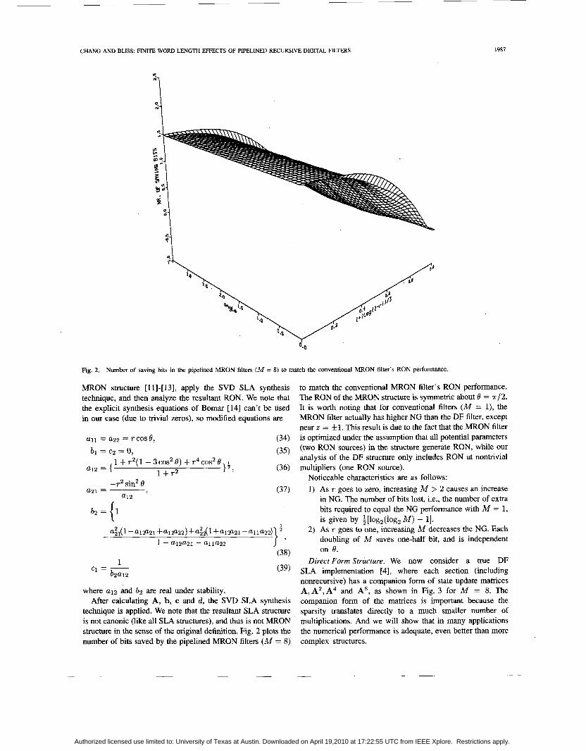
Fig. 2. Number of saving bits in the pipelined MRON filters ( M = 8) to match the conventional MRON filter's RON performance.

MRON structure [Ill-[13], apply the SVD SLA synthesis technique, and then analyze the resultant RON. We note that the explicit synthesis equations of Bomar [14] can't be used in our case (due to trivial zeros), so modified equations are

- r2 sin2 6 a21 = ,

a12 (37)

b2={l

1 c1 = -

b2a12 (39)

where a12 and b2 are real under stability. After calculating A, b, c and d , the SVD SLA synthesis

technique is applied. We note that the resultant SLA structure is not canonic (like all SLA structures), and thus is not MRON structure in the sense of the original definition. Fig. 2 plots the number of bits saved by the pipelined MRON filters ( M = 8)

to match the conventional MRON filter's RON performance. The RON of the MRON structure is symmetric about 6' = 7r/2. It is worth noting that for conventional filters ( M = l), the MRON filter actually has higher NG than the DF filter, except near z = f l . This result is due to the fact that the MRON filter is optimized under the assumption that all potential parameters (two RON sources) in the structure generate RON, while our analysis of the DF structure only includes RON at nontrivial multipliers (one RON source).

Noticeable characteristics are as follows: 1) As T goes to zero, increasing M > 2 causes an increase

in NG. The number of bits lost, i.e., the number of extra bits required to equal the NG performance with M = 1, is given by

2) As T goes to one, increasing M decreases the NG. Each doubling of M saves one-half bit, and is independent on B.

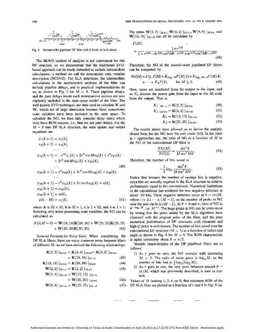
Direct Form Structure. We now consider a true DF SLA implementation [4], where each section (including nonrecursive) has a companion form of state update matrices A,A2,A4 and A8, as shown in Fig. 3 for M = 8. The companion form of the matrices is important because the sparsity translates directly to a much smaller number of multiplications. And we will show that in many applications the numerical performance is adequate, even better than more complex structures.

[log,(log, M ) - 11.


1988 IEEE TRANSACXIONS ON SIGNAL PROCESSING, VOL. 42, NO. 8, AUGUST 1994

1 1 1

e&)

Fig. 3. Second-order pipelined DF filter with 8 levels of look-ahead.

The SKWD method of analysis is not convenient for this DF structure, so we demonstrate that the traditional SVD- based approach can be easily extended to include intermediate calculations, a method we call the noncanonic state variable description (NCSVD). For SLA structures, the intermediate calculations in the nonrecursive sections of the filter can include pipeline delays, and in practical implementations do so, as shown in Fig. 3 for M = 8. These pipeline delays, and the pure delays inside each nonrecursive section are now explicitly included in the state-space model of the filter. The well known SVD techniques are then used to calculate K and W, which are of large dimension because these noncanonic state variables have been included in the state space. To calculate the NG, we then only consider those states which truly have RON sources, i.e., that are not pure delays. For the M = 8 true DF SLA structure, the state update and output equations are

z l ( k + 1) = 2 2 ( k ) ,

m ( k + 1) = 2 3 ( k ) , ..

2 3 o ( k + 1) = T 2 2 3 1 ( k ) + 2TCOS6232(k) + U(k), 231(k + 1) = z32(k),

232(k + 1) = U(k), ~ ( k - 16) = ~ l ( k ) (41)

where A is 32 x 32, b is 32 x 1, c is 1 x 32, and d is 1 x 1. Selecting only noise generating state variables, the NG can be calculated as

NG(M = 8 ) = W(16,16)K(16,16) + W(25,25)K(25,25)

+ W(3O,30)K(3O7 30). (42)

General Formula for Noise Gain. When considering the DF SLA filters, there are many common terms between filters of different M, so we have derived the following relationships:

K(2,2) 1M=i = K(4,4) ~ M = z = K(8,8) I M = ~ = K(16,16) 1 ~ = 8 (43)

(44) (45)

= W(30,30) I M = ~ (46) (47)

K(13,13) I M = ~ = K(30,30) ( M = S

w(272) IM=l = K(272) lM=l w ( 4 , 4 ) / M = Z = w(13,13) I M = ~

W(8,8) 1 ~ ~ 4 = W(25,25) l h . 1 ~ 8

The terms W(2,2) l ~ = 1 , W ( 4 , 4 ) 1 ~ 4 = ~ , W ( 8 , 8 ) IM=~, and W(16,16) 1 ~ = 8 can all be calculated by

P(M) - 1+TzM -

1 + TZM -4T2MCOS2M6-T4M +4T4MCOS2M6-T6M ' (48)

Therefore, the NG of the second-order pipelined DF filters can be computed by

NG(M) = P(1, P(M) + K ~ o g , M P ( M/2) + Klog, M - 1P(M/4) + . - . + K z P ( 2 ) , for M 2 2. (49)

Here, states are numbered from the output to the input, and so Ki denotes the power gain from the input to the ith node from the output. That is,

(50) (51)

K2 = K(13,13) 1 ~ = 4 , (52) K3 = K(25,25) l ~ = 8 . (53)

The results above have allowed us to derive the analytic closed form for the NG near the unit circle [15]. In the limit as T approaches one, the ratio of NG as a function of M to the NG of the conventional DF filter is

Ki 1M=i = K(2,2) lM=i, K1 lM=2 = K(4,4) 1M=2,

N G ( M ) = sin26

NG( 1) Therefore, the number of bits saved is

M sin2 M0 '

1 sin2 6 - 2 log, M MO '

(54)

(55 )

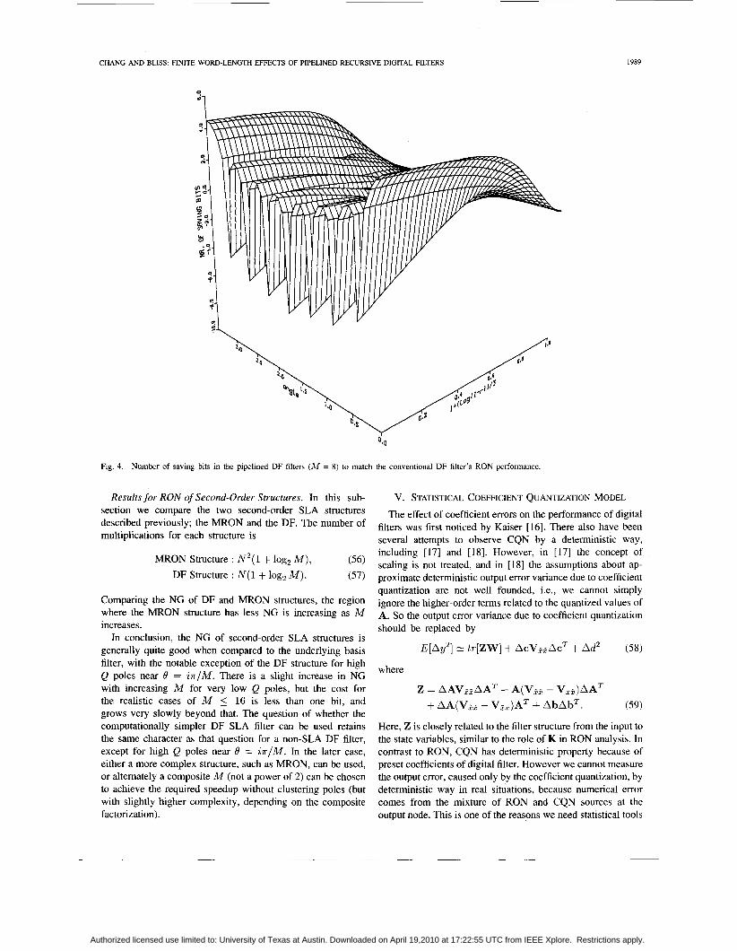
Notice that because the number of savings bits is negative, extra bits are actually required in the SLA structure to achieve performance equal to the conventional. Numerical limitations in the calculations has rendered the true negative infinities at about -50 bits. These negative infinities occur at 6 = i.rr/M, where i = f l . . . f ( M - 1), so the number of peaks in NG near the unit circle is ( M - 1). At 6 = 0 and 7r, ratio of NG is 8- log, M , i.e. M - 3 . The huge peaks in NG can be understood by noting that the poles added by the SLA algorithm have clustered with the original poles of the filter, and the poor numerical performance of DF structures with clustered and high Q poles is well known. The number of bits saved over the conventional DF structure ( M = 1) as a function of radius and angle is shown in Fig. 4 for M = 8. The RON characteristic is again symmetric about 6 = .rr/2.

Notable characteristics of the DF pipelined filters are as follows:

1) As T goes to zero, the NG worsens with increasing M > 2. The ratio of noise gains is log, M , so the number of bits lost is $log,(log, M ) .

2) As T goes to one, the very poor behavior around 6 = i x / M , which was previously described, is seen in con- text.

Values of M (among 1, 2, 4, or 8) that minimize RON of the DF SLA filter are plotted as a function of T and 6 in Fig. 6 (a).



“I

Fig. 4. Number of saving bits in the pipelined DF filters ( M = 8) to match the conventional DF filter’s RON performance.

Results for RON of Second-Order Structures. In this subsection we compare the two second-order SLA structures described previously; the MRON and the DF. The number of multiplications for each structure is

MRON Structure : N2(1 + log, M ) , DF Structure : N(l + log, M ) .

(56) (57)

Comparing the NG of DF and MRON structures, the region where the MRON structure has less NG is increasing as M increases.

In conclusion, the NG of second-order SLA structures is generally quite good when compared to the underlying basis filter, with the notable exception of the DF structure for high Q poles near 6 = i r / M . There is a slight increase in NG with increasing M for very low Q poles, but the cost for the realistic cases of M 5 16 is less than one bit, and grows very slowly beyond that. The question of whether the computationally simpler DF SLA filter can be used retains the same character as that question for a non-SLA DF filter, except for high Q poles near 0 = i r / M . In the later case, either a more complex structure, such as MRON, can be used, or altemately a composite M (not a power of 2 ) can be chosen to achieve the required speedup without clustering poles (but with slightly higher complexity, depending on the composite factorization).

V. STATISTICAL COEFFICIENT QUANTIZATION MODEL

The effect of coefficient errors on the performance of digital filters was first noticed by Kaiser [16]. There also have been several attempts to observe CQN by a deterministic way, including [17] and [18]. However, in [17] the concept of scaling is not treated, and in [18] the assumptions about ap- proximate deterministic output error variance due to coefficient quantization are not well founded, i.e., we cannot simply ignore the higher-order terms related to the quantized values of A, So the output error variance due to coefficient quantization should be replaced by

E[Ay2] N tr[ZW] + AcV,j:Ac’ + Ad2 (58)

where

Z = AAV,,AAT + A(V22 - Vx2)AAT + AA(V22 - VzX)AT + AbAbT. (59)

Here, Z is closely related to the filter structure from the input to the state variables, similar to the role of K in RON analysis. In contrast to RON, CQN has deterministic property because of preset coefficients of digital filter. However we cannot measure the output error, caused only by the coefficient quantization, by deterministic way in real situations, because numerical error comes from the mixture of RON and CQN sources at the output node. This is one of the reasons we need statistical tools



to analyze CQN. Another reason is the necessity of unifying analytical and synthetic tools for both errors. Methods using statistical analysis for coefficient quantization include [ 181- [22]. Fettweis noticed there exists similarity of generations between RON and CQN [ 191. According to Jackson [ 131, RON and CQN are found to form the bound of each other. Recently two noticeable researches about statistical CQN (SCQN) have been done in [20] and [21], and they reach the same conclusion even though they employed different approaches.

In this paper, we provide another viewpoint for the analysis of CQN. That is, to calculate the reflected CQN on the output node, output noise power due to coefficient quantization, a&QN, is considered instead of coefficient sensitivity. In a&QN analysis with supporting register model, the amount of output error can be directly found. There also has been an attempt to find the linear dependence between the weighted sensitivity and the weighted noise measure [22].

In the following sections, we apply the state-space linear algebraic approach for RON analysis of [ l l ] to the coefficient quantization problem. Statistical assumptions including hardware model to unify the CQN and RON analysis are also presented. The SLA filters with the power-of-two decomposition in [4] are used as an example structure to demonstrate a unified approach. These results contradict previous claims [6] about the numerical performance of the SLA structure, where register scaling [8], [23] was not considered. The total output error variance after applying a proper scaling is derived by combining RON and CQN [24].

In this section we state sufficient conditions to show that SCQN source scan be interpreted just like single-length accumulation RON source. This result was also achieved in [21] by assuming certain approximations, and as a different form in [20]. In [21] by using the state error vector e,(IC) = Z ( k ) - o(k) and the output error ey(lc) = y(k) - y(k), the statistical sensitivity S, output error variance normalized by the variance o2 of coefficient variations, is described by

S = ogQN/a2 = tr[K]tr[W] + tr[W] + t r [K] (60)

where output branch is omitted as usual. Here, it is assumed all the elements of the system matrices are varied and

K = K (61)

where K is the state covariance matrix of the ideal filter and K is that of the quantized filter. For (61), the condition o2 << o:, where o: is an upper bound of variance that satisfies mean square asymptotical stability of the virtual system, should be satisfied. Another underlying assumption in (60) is the same q for state vector and system matrices A, b, c and d, that means there are the same length of bits below decimal point in every register. A, in defining quantization step size q, is a constant chosen to fit the dynamic range of signal. However, A for state vector and system matrices does not usually have the same values (A for state vector is 1 by using the Z2-scaling with S = 1). That is, A and B combination of state vector and system matrices should be different to guarantee the same q. Therefore, the number of bits above the decimal point for system matrices should be determined

e.

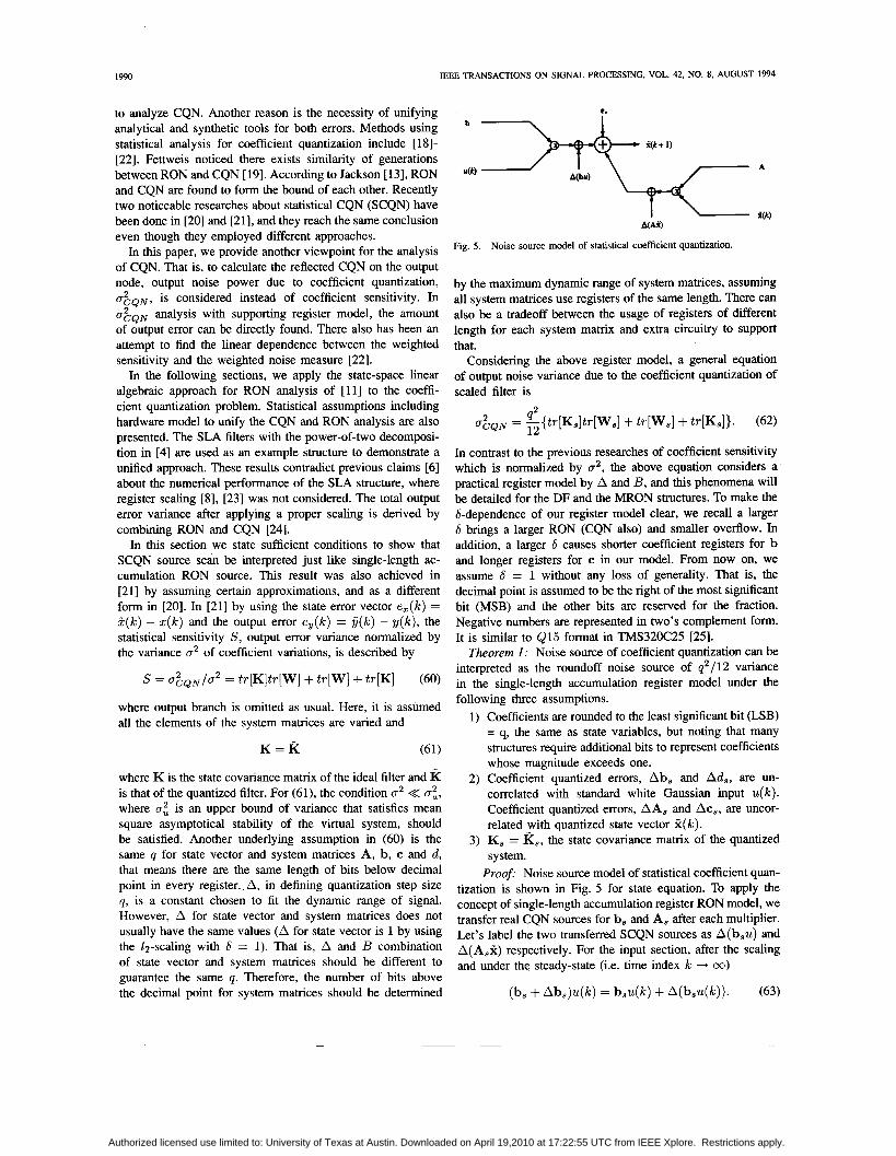
Fig. 5. Noise source model of statistical coefficient quantization.

by the maximum dynamic range of system matrices, assuming all system matrices use registers of the same length. There can also be a tradeoff between the usage of registers of different length for each system matrix and extra circuitry to support that.

Considering the above register model, a general equation of output noise variance due to the coefficient quantization of scaled filter is

q' &QN = ~ { t ~ [ K s ] t r [ W s ] + tr[W,] + tr[K,]}. (62)

In contrast to the previous researches of coefficient sensitivity which is normalized by a', the above equation considers a practical register model by A and B, and this phenomena will be detailed for the DF and the MRON structures. To make the &dependence of our register model clear, we recall a larger 6 brings a larger RON (CQN also) and smaller overflow. In addition, a larger 6 causes shorter coefficient registers for b and longer registers for c in our model. From now on, we assume S = 1 without any loss of generality. That is, the decimal point is assumed to be the right of the most significant bit (MSB) and the other bits are reserved for the fraction. Negative numbers are represented in two's complement form. It is similar to Q15 format in TMS320C25 [25].

Theorem I : Noise source of coefficient quantization can be interpreted as the roundoff noise source of q2/12 variance in the single-length accumulation register model under the following three assumptions.

1) Coefficients are rounded to the least significant bit (LSB) = q, the same as state variables, but noting that many structures require additional bits to represent coefficients whose magnitude exceeds one.

2) Coefficient quantized errors, Ab, and Ad,, are uncorrelated with standard white Gaussian input u(lc). Coefficient quantized errors, AA, and Ac,, are uncorrelated with quantized state vector $ ( I C ) .

3) K, = K,, the state covariance matrix of the quantized system.

Proof: Noise source model of statistical coefficient quantization is shown in Fig. 5 for state equation. To apply the concept of single-length accumulation register RON model, we transfer real CQN sources for b, and A, after each multiplier. Let's label the two transferred SCQN sources as A(b,u) and A(A,X) respectively. For the input section, after the scaling and under the steady-state (i.e. time index IC + CO)

(b, + Ab,)u(k) = b,u(k) + A(b,u(k)). (63)


CHANG AND BLISS: FINITE WORD-LENGTH EFFECTS OF PIPELINED RECURSIVE DIGITAL RLTERS 1991

That is,

Therefore, the variance of A(b,u(k)) becomes

2 aA(bs ~ ( k ) )

N E [ A b, A by] E [U, I] - E [ Ab,] E [U] E [ U] E [ Ab,] T ,

= -1. 12

= E[Ab,AbT. u'I] - E[Ab, . u]E[Ab, . u ] ~ ,

(65) q2

Here, we used the assumption of uncorrelation between Ab, and U. For the state recurrence section,

(A, + AA,)X(k) = A,X(k) + A(A,x(k)). (66)

Then

A(A,X(k)) = AA, . X ( k ) . (67)

Therefore, the variance of A(A,X(k)) becomes

a&As%(k))

= E[AA,AAy . X X T ] - E[AA, . X]E[AA, . X I T ,

N E[AA,AAT]E[Xji.'] - E[AAs]E[X]E[X]'E[AAs]T,

- -E[XXT], q2 - 12

= -1. 12 q2

Here, we used the assumption that AA, and x are uncorrelated with each other and K, is equal to K,, the state covariance matrix of quantized filter. Above derivations are similarly applied to the output equation. Therefore, the variances of all noise sources are proved to be q2/12 in our SCQN model. 0

The above three assumptions assure the variance of each noise source of single-length accumulation register is equal to q2/12, and are the same assumptions as those in [21] except the first one. Actually, the first assumption has not been noticed before, but it was represented as a normalized output error variance instead. For the compactness of the theorem, we assumed state variables and coefficients are all rounded to the L S B = q together. However, even though state variables and each coefficient have different quantization step sizes, the actual value of can be directly calculated in our model under the validity of assumptions 2 and 3. In the previous researches of CQN sensitivity, it was difficult to calculate the value of a:QN, even in the case of same q, unless we know the variance of coefficient variations, which cannot easily be obtained from the specifications of a digital filter.

The main point of the above analysis is the unification of analysis methods for RON and CQN. Moreover, the min-

imization of RON also ensures the minimization of CQN, that is, the minimization of numerical noises can be achieved simultaneously under the assumption of full system matrix. The above analyses are based on the condition of mean square asymptotical stability of the quantized filter which guarantees the convergence of state covariance matrix and state error covariance matrix of quantized filter 1211.

The accuracy of (60) was considered in detail in [21]. For the DF filter, we consider the sparsity of A, matrix also. The largest values of coefficients come from c if 6 2 1,which is a usual case. For the our all-pole second-order filters, it is

which is a. It is the same for the DF and the MRON filters and also the same for all levels of loop pipelined filters. That is, (69) can also be the extra bits for the pipelined filters. It is interesting to note that the maximum value of A, in the DF filter is always larger than 1 (0 for extra bits), but always smaller than 1 in the MRON filter. We observe the dynamic range of b, over the z-plane in the DF filter has significantly larger value than in the MRON filter, and the maximum values of b, of both filters are less than 1.

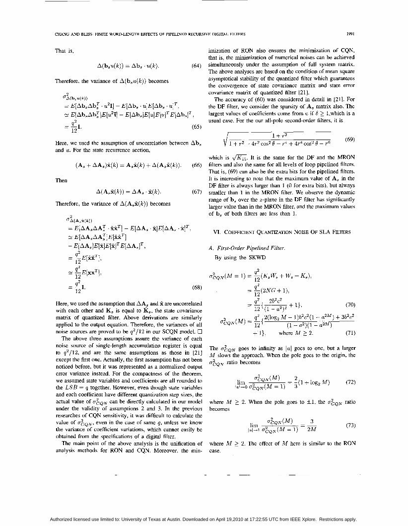
VI. COEFFICIENT QUANTIZATION NOISE OF SLA FILTERS

A . First-Order Pipelined Filter.

By using the SKWD

q2 2(10g2 M - 1)b2c2(1 - u Z M ) + 3b2c2 (1 - u2)(1- .2M 1 &N(M) = E{

+ 1}, where M 2 2. (71)

The u ~ Q N goes to infinity as la1 goes to one, but a larger M slows the approach. When the pole goes to the origin, the

ratio becomes

where M 2 2. When the pole goes to f l , the a&QN ratio becomes

(73)

where M 2 2. The effect of M here is similar to the RON case.



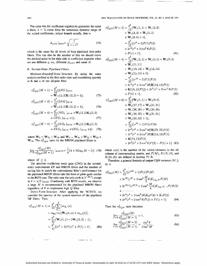
The extra bits for coefficient registers to guarantee the same q (here, S = 1) come from the maximum dynamic range of the scaled coefficients, output branch usually, that is

(74)

which is the same for all levels of loop pipelined first-order filters. This can also be the number of bits we should move the decimal point to the right side in coefficient registers when we use different 4, i.e., different Acoff and same B.

agQN(M = 4) = QC{W,(l, 1) + W,(5,5) + W,(9,9) 12

+ W,(ll, 11) B. Second-Order Pipelined Filters + W,(13,13) + W,(14,14)

Minimum Roundoff Noise Structure. By using the same analysis method in the first-order case and considering sparsity in b and c of our all-pole filter

+ W,(15,15) + l}, = -{(r16 q2 + l)P(l)P(4)

12 + 2r4(r4 + 2cOs2 z e ) ~ ( i 3 , i 3 ) ~ ( 4 )

+ P(1) + 11, (82)

+ K(13,13)P(2) + 2r2(r2 + 2c0s2 B)P(2)

q2 o ~ Q N ( M = 8) = -{Ws(l, 1) + Ws(9,9) 12 + w5(17, 17) + w,(21, 21)

+Ws(26,26)+W,(28,28) + W,(30,30) + W,(31,31)

where W2 = Wzl+ W22 and W3 = w31+ w32 + W33 + W34. The agQN ratio for the MRON pipelined filters is

where M 2 2. The absolute coefficient noise gain (CNG) in the second-

order conventional DF and MRON filters and the number of saving bits to match the conventional filter’s performance for the pipelined MRON filters take the form of plots quite similar to the RON case. The ratio near the unit circle is 2-M/4, except at B = 7 ~ / 2 ( ~ = 2 . Combining with RON results, we observe a large M is recommended for the pipelined MRON filters regardless of 0 to implement high Q filter.

Direct Form Structure. After applying the NCSVD, we consider the sparsity of the system matrices of the pipelined DF filters. Then,

2 2

agQN(M = 1) = “{E( mA, (n) n = l

12

+ 2r4(r4 + 2 ~ 0 s ~ ~ B ) K ( I ~ , i 3 ) ~ ( 4 )

+ K(13,13)P(2) + 2r2(r2 + 2c0s2 B)P(2) + P(1) + l} (83)

where m(i) is the number of the varied elements in the ith column of corresponding matrix, and P ( M ) , K ( 13,13), and K(25,25) are defined in Section IV-B.

Therefore, a general formula of output CQN variance ( M 2 4) is

q2 &QN(M) = -{(r4M + l)P(l)P(M) 12

M 2

+ 2rM(rM + 2 cos2 -B)Klog, M P ( M )

M 4

+ 2rM/2(rM/2 + 2c0s2 - B ) K l O g , MP1P(M/2) + . . . . . . . . . + 2r4(r4 + zcOs2 20)&P(4) + ~ ~ ~ ( 2 1 + 2r2(r2 + 2c0s2 e ) ~ ( 2 ) + ~ ( 1 ) + 1). (84)

Then the agQN ratio becomes



1 .o

0.5

g o

-0.5

- 1 .o -

M-1 : M-2 : M-4 : M-8 :

0.5 1 .o - 1 .o ' ' ' ' ' ' I ' L(; , ' ' ' ' ' ' - 1 . 0 -0.5

M - 1 :

M = 2 : . M = 4 : x

M = 8 : - REAL

(b)

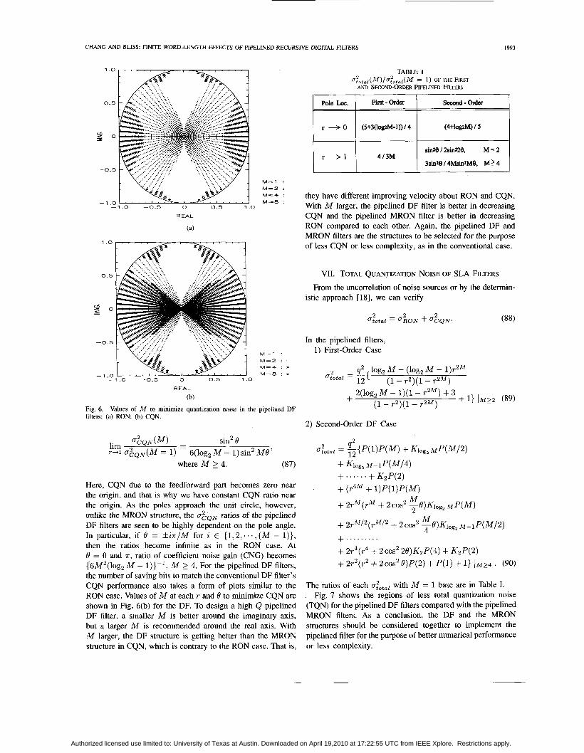
Fig. 6. filters: (a) RON (b) CQN.

Values of ,I.I to minimize quantization noise in the pipelined DF

o&QN(') - sin2 e lim - r+1 o g Q N ( M = 1) 6(log, M - 1) sin2 MO'

where M 2 4. (87)

Here, CQN due to the feedforward part becomes zero near the origin, and that is why we have constant CQN ratio near the origin. As the poles approach the unit circle, however, unlike the MRON structure, the ~7.6~ ratios of the pipelined DF filters are seen to be highly dependent on the pole angle. In particular, if 0 = f i ~ / M for i E ( 1 ' 2 , . ... ( M - l)}, then the ratios become infinite as in the RON case. At 19 = 0 and T , ratio of coefficient noise gain (CNG) becomes {6M2(log2 M - l)}-', M 2 4. For the pipelined DF filters, the number of saving bits to match the conventional DF filter's CQN performance also takes a form of plots similar to the RON case. Values of M at each T and 6 to minimize CQN are shown in Fig. 6(b) for the DF. To design a high Q pipelined DF filter, a smaller M is better around the imaginary axis, but a larger M is recommended around the real axis. With M larger, the DF structure is getting better than the MRON structure in CQN, which is contrary to the RON case. That is,

TABLE I

AND SECOND-ORDER PPELINED FILTERS O~ot,,(M)/U~ota,(M = 1) OFTHE FIRST

(4+logzM) I 5

they have different improving velocity about RON and CQN. With M larger, the pipelined DF filter is better in decreasing CQN and the pipelined MRON filter is better in decreasing RON compared to each other. Again, the pipelined DF and MRON filters are the structures to be selected for the purpose of less CQN or less complexity, as in the conventional case.

VII. TOTAL QUANTIZATION NOISE OF SLA FILTERS

From the uncorrelation of noise sources or by the deterministic approach [18], we can verify

In the pipelined filters, 1) First-Order Case

2(10g2 M - 1)(1 - r Z M ) + 3 + 11 IM22 (89) ( 1 - T 2 ) ( 1 - T 2 M ) +

2) Second-Order DF Case

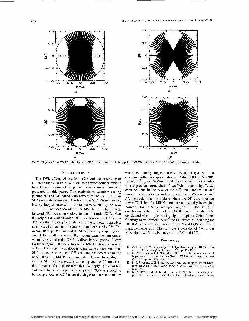
The ratios of each ototal with M = 1 base are in Table I. Fig. 7 shows the regions of less total quantization noise

(TQN) for the pipelined DF filters compared with the pipelined MRON filters. As a conclusion, the DF and the MRON structures should be considered together to implement the pipelined filter for the purpose of better numerical performance or less complexity.


IEEE TRANSACTIONS ON SIGNAL PROCESSING, VOL. 42, NO. 8, AUGUST 1994 1993

1 .o 1 .o

0.5 0.5

cj w s o s o -0.5 -0.5

- 1 .o -1.0 -0.5 0 0.5 1 . 0 -1 .o

- 1 . 0 -0.5 0 0.5 1 . 0

0.5

w s o -0.5

0.5

-0.5

Fig 7 Region of less TQN for the pipelined DF filters compared with the pipelined MRON filters (a) .11=1, (b) 11=2, (c) -11=4, (d) 11=8

VIII. CONCLUSIONS

The FWL effects of the first-order and the second-order DF and MRON-based SLA filters using fixed-point arithmetic have been investigated using the unified statistical methods presented in this paper. Two methods to calculate scaling parameters and NG ratios with respect to the M = 1 (non- SLA) were demonstrated. The first-order SLA forms increase NG by log,M near z = 0, and decrease NG by M near z = kl. The second-order SLA MRON form has a well behaved NG, being very close to the first-order SLA. Near the origin the second-order DF SLA has constant NG, but depends strongly on pole angle near the unit circle, where NG ratios vary between infinite increase and decrease by M 3 . The overall RON performance of the SLA pipelining is quite good, except for small regions of the z-plane near the unit circle, where the second-order DF SLA filters behave poorly. Except for these regions, the need to use the MRON structure instead of the DF structure is analogous to the same choice with non- SLA filters. Because the DF structure has fewer summing nodes than the MRON structure, the DF can have slightly smaller NG in certain regions of the z-plane. As M increases, this region of the z-plane atrophies. By applying the unified statistical tools developed in this paper, CQN is proved to be interpretable as RON under the single-length accumulation

model and usually larger than RON in digital system. In our modeling with given specifications of a digital filter, the actual value of ngQN can be directly calculated, which is not possible in the previous researches of coefficient sensitivity. It can even be done in the case of the different quantization step sizes for state variables and each coefficient. With increasing M , the regions in the z-plane where the DF SLA filter has lower CQN than the MRON structure are actually increasing; however, for RON the analogous regions are decreasing. In conclusion, both the DF and the MRON basis filters should be considered when implementing high throughput digital filters. Contrary to widespread belief, the DF structure including the DF SLA, sometimes exhibits lower RON and CQN with lower implementation cost. The limit cycle behavior of the various SLA pipelined filters is analyzed in [26] and [27].

REFERENCES

[ l ] A. L. Moyer, “An efficient parallel algorithm for digital IIR filters,” in Proc. IEEE Int. Conf. ASSP, Apr. 1976, pp. 525-528.

[2] C. W. Bames and S. Shinnaka, “Block shift invariance and block implementation of discrete-time filters,” IEEE Truns. Circuits Syst., vol.

131 R. P. Brent and 2. B. Bing, “A stabilized parallel algorithm for direct- form recursive filters,” IEEE Trans. Comput., vol. 40, pp. 333-336, Mar. 1991.

[4] K. K. Parhi and D. G. Messerschmitt, “Pipeline interleaving and parallelism in recursive digital filters, Part I : Pipelining using scattered

CAS-27, pp. 667-672, Aug. 1980.


CHANG AND BLISS: FINITE WORDLENGTH EFFECTS OF PIPELINED RECURSIVE DIGITAL FILTERS 1995

look-ahead and decomposition,” IEEE Trans, Acoust., Speech, Signal Processing, vol. 37, pp. 1099-1 117, July 1989.

[5 ] I. G. Chung and K. K. Parhi, “Design of pipelined lattice IIR digital filters,” in Proc. Asilomar Conf., Nov. 1991, pp. 1021-1025.

[6] K. K. Parhi, “Finite word effects in pipelined recursive filters,” IEEE Trans. Signal Processing, vol. 39, pp. 1450-1454, June 1991.

[7] R. A. Roberts and C. T. Mullis, Digital Signal Processing. Reading, MA: Addison-Wesley, 1987.

[SI W. G. Bliss and K. H. Chang, “The roundoff noise of pipelined scattered look-ahead W digital filters with decomposition,” in Proc. Asilomar Conf., Nov. 1991, pp. 1026-1030.

[9] Y. C. Lim and B. Liu, “Pipelined recursive filter with minimum order

[25] Texas Instruments, TMS32OC25 Digital Signal Processor Design Work- shop, ver. 4.0, Nov. 1989.

[26] K. H. Chang and W. G. Bliss, “Limit cycles in state-space pipelined scattered look-ahead filters,” in Proc. IEEE 35rh Midwest Symp. on Circuits Syst., Aug. 1992, pp. 1128-1131.

[27] -, “Limit cycle behavior of pipelined recursive digital filters,” IEEE Trans. Circuits Syst., vol. 41, pp. 351-355, May 1994.

augmentation,” IEEE Trans. Acoust., Speech, Signal Processing, vol.

[lo] C . D. Thompson, “Area-time complexity for VLSI,” in Proc. Caltech Conf on V a l , Jan. 1979, pp. 495-508.

[ 111 C. T. Mullis and R. A. Roberts, “Synthesis of minimum roundoff noise fixed point digital filters,” IEEE Trans. Circuits Syst., vol. CAS-23, pp. 551-562, Sept. 1976.

[12] S. Y. Hwang, “Minimum uncorrelated unit noise in state-space digital filtering,” IEEE Trans. Acoust., Speech, Signal Processing, vol.

[13] L. B. Jackson, A. G. Lindgren, and Y. Kim, “Optimal synthesis of second-order state-space structures for digital filters,’’ IEEE Trans. Circuits Syst., vol. CAS-26, pp. 149-153, Mar. 1979.

[14] B. W. Bomar, “New second-order state-space structures for realizing low roundoff noise digital filters,” IEEE Trans. Acoust., Speech, Signal Processing. vol. ASSP-33, pp. 106-1 10, Feb. 1985.

[15] K. H. Chang, “Finite word-length effects of pipelined recursive digital filters,” Ph.D. Dissertation, Dept. Elec. Eng., Texas A&M Univ., Aug. 1992.

[I61 J. F. Kaiser, “Some practical considerations in the realization of linear digital filters,” in Proc. 3rd Allerton Conf. on Circuit and Syst. Theory,

[17] J. B. Knowles and E. M. Olcayto, “Coefficient accuracy and digital filter response,” IEEE Trans. Circuit Theory, vol. CT-15, pp. 3141, Mar. 1968.

40, pp. 1643-1651, July 1992.

ASSP-25, pp. 273-281, Aug. 1977.

pp. 621-633, Oct. 1965.

M. Kawamata and T. Higuchi, “A unified approach to the optimal synthesis of fixed-point state-space digital filters,” IEEE Trans. Acoust., Speech, Signal Processing, vol. ASSP-33, pp. 911-920, Aug. 1985. A. Fettweis, “On the connection between multiplier word length limita- tion and roundoff noise in digital filters,” IEEE Trans. Circuit Theory,, vol. CT-19, pp. 486491, Sept. 1972. V. Tavsanoglu and L. Thiele, “Optimal design of state-space digital filters by simultaneous minimization of sensitivity and roundoff noise,” IEEE Trans. Circuits Syst., vol. CAS-31, pp. 884-888, Oct. 1984. M. Iwatsuki, M. Kawamata, and T. Higuchi, “Statistical sensitivity and minimum sensitivity structures with fewer coefficients in discrete time linear systems,” IEEE Trans. Circuits Syst., vol. 37, pp. 72-80, Jan. 1990.

[22] L. Thiele, “On the sensitivity of linear state-space systems,” IEEE Trans. Circuits Syst., vol. CAS-33, pp. 502-510, May 1986.

[23] K. H. Chang and W. G. Bliss, “Register modeling for the unification of quantization analysis in IIR digital filters,” in Proc. Asilomqr Conf.,

[24] -, “Roundoff and coefficient quantization noise of pipelined scattered look-ahead filters with decomposition,” in Proc. IEEE Inc. Cont. Acoust., Speech, Signal Processing, Mar. 1992, vol. 4, pp. 433-436.

Oct. 1992, pp. 278-282.

KyungHi Chang (S’87-M’92) was bom in Yesan, Korea, in 1962. He received the B.S. and M.S. degrees in electronics engineering from the Yonsei University, Seoul, in 1985 and 1987, respectively. He received the Ph.D. degree in electrical engineering from the Texas A&M University, College Station, in 1992.

From 1989 to 1990, he was with Samsung Ad- vanced Institute of Technology (SAIT), Kihung, Korea, as a Researcher, and was involved in the DSP system design of a home-use digital VCR. In

1992, he joined the Integrated Circuits D&elopment Section of Electronics and Telecommunications Research Institute (ETRI), Taejon, Korea, as a Senior Researcher, and is currently implementing CDMA system. His research inter- ests include digital filter design and performance analysis, parallel architecture, VLSI signal processing, VLSI systems design, and mobile communication system design. Dr. Chang is a member of the IEEE Signal Processing, Circuits and

Systems, and Communications Societies.

design. He was a cons1 dt

William G. Bliss (S’88-M’89) received the B.S. degree from South Dakota State University in 1975, the M.S. degree from the University of Minnesota in 1975, and the Ph.D. degree from the University of Colorado at Boulder in 1988, all in electrical engineering.

He was with the IBM Development Labs in Rochester, MN, and Boulder, CO from 1977-1983, working on various aspects of magnetic recording including modulation coding, error correction coding, phase-locked loop design, and optimal reciever ant to Saxpy Computer Corp. from 1987 to 1988 in

the areas of fault-tolerant array computing and parallel algorithms for moving image sequence estimation. He served a four-year term on the faculty of Texas A&M University, Department of Electrical Engineering, from 1988 to 1992, where his research included parallel algorithms for digital signal processing, finite arithmetic effects in digital signal processing, and digital control of analog signal processing circuits. He joined the technology group of Cirrus Logic, Broomfield, CO, in 1992, where he works on VLSI architectures for magnetic recording read channels.


Documents

Finite word-length effects of pipelined recursive digital ...users.ece.utexas.edu/~adnan/comm/chang-bliss-sqnr-94.pdf · Finite Word-Length Effects of Pipelined Recursive Digital