Finite Mixture Models and Clustering - College of … · Finite Mixture Models and Clustering Mohamed Nadif LIPADE, Université Paris Descartes, France Nadif (LIPADE) EPAT, May, 2010

Finite Mixture Models and Clustering

Mohamed Nadif

LIPADE, Université Paris Descartes, France

Nadif (LIPADE) EPAT, May, 2010 Course 3 1 / 40

Introduction

Outline

1 Introduction

Mixture Approach

2 Finite Mixture Model

Definition of the modelExampleDifferent approaches

3 ML and CML approaches

EM algorithmCEM algorithmOthers variants of EM

4 Applications

Gaussian mixture modelBernoulli mixtureMultinomial Mixture

5 Model Selection

6 Conclusion


Introduction Mixture Approach

Classical clustering methods

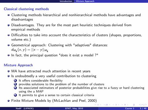
Clustering methods hierarchical and nonhierarchical methods have advantages anddisadvantages

Disadvantages. They are for the most part heuristic techniques derived fromempirical methods

Difficulties to take into account the characteristics of clusters (shapes, proportions,volume etc.)

Geometrical approach: Clustering with "adaptives" distances:dMk

(x , y) = ||x − y ||Mk

In fact, the principal question "does it exist a model ?"

Mixture Approach

MA have attracted much attention in recent years

Is undoubtedly a very useful contribution to clustering1 It offers considerable flexibility2 provides solutions to the problem of the number of clusters3 Its associated estimators of posterior probabilities give rise to a fuzzy or hard clustering

using the a MAP4 It permits to give a sense to certain classical criteria

Finite Mixture Models by (McLachlan and Peel, 2000)


Finite Mixture Model

Outline

1 Introduction

Mixture Approach





4 Applications


5 Model Selection

6 Conclusion


Finite Mixture Model Definition of the model

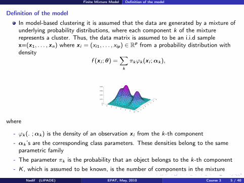
Definition of the model

In model-based clustering it is assumed that the data are generated by a mixture ofunderlying probability distributions, where each component k of the mixturerepresents a cluster. Thus, the data matrix is assumed to be an i.i.d samplex=(x1, . . . , xn) where x i = (xi1, . . . , xip) ∈ R

p from a probability distribution withdensity

f (x i ; θ) =∑

k

πkϕk(x i ; αk),

−4−2

02

46

810 −3

−2−1

01

23

4

0

0.02

0.04

0.06

0.08

where

- ϕk(. ; αk) is the density of an observation x i from the k-th component

- αk ’s are the corresponding class parameters. These densities belong to the sameparametric family

- The parameter πk is the probability that an object belongs to the k-th component

- K , which is assumed to be known, is the number of components in the mixture


Finite Mixture Model Example

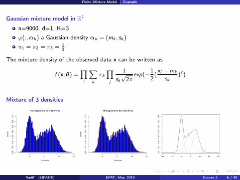
Gaussian mixture model in R1

n=9000, d=1, K=3

ϕ(., αk) a Gaussian density αk = (mk , sk)

π1 = π2 = π3 = 13

The mixture density of the observed data x can be written as

f (x;θ) =∏

i

∑

k

πk

∏

j

1

sk√

2πexp(−1

2(xi − mk

sk)2)

Mixture of 3 densities

Histogramme des données

Données

Dens

ité

0 5 10 15

0.00

0.02

0.04

0.06

0.08

0.10

0.12

0.14

Histogramme des données

Données

Dens

ité

0 5 10 15

0.00

0.02

0.04

0.06

0.08

0.10

0.12

0.14

−10 −5 0 5 10 15 200.

000.

020.

040.

060.

080.

100.

120.

14


Finite Mixture Model Example

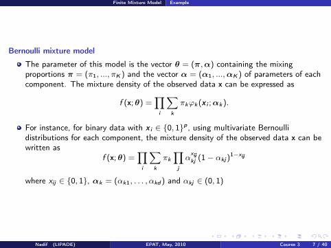
Bernoulli mixture model

The parameter of this model is the vector θ = (π, α) containing the mixingproportions π = (π1, ..., πK ) and the vector α = (α1, ..., αK ) of parameters of eachcomponent. The mixture density of the observed data x can be expressed as

f (x;θ) =∏

i

∑

k

πkϕk(x i ; αk).

For instance, for binary data with x i ∈ {0, 1}p , using multivariate Bernoullidistributions for each component, the mixture density of the observed data x can bewritten as

f (x; θ) =∏

i

∑

k

πk

∏

j

αxij

kj (1 − αkj )1−xij

where xij ∈ {0, 1}, αk = (αk1, . . . , αkd ) and αkj ∈ (0, 1)


Finite Mixture Model Different approaches

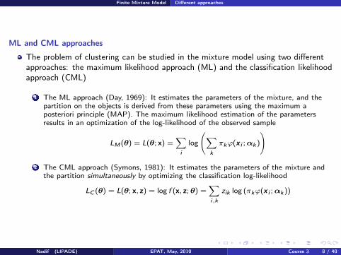
ML and CML approaches

The problem of clustering can be studied in the mixture model using two differentapproaches: the maximum likelihood approach (ML) and the classification likelihoodapproach (CML)

1 The ML approach (Day, 1969): It estimates the parameters of the mixture, and thepartition on the objects is derived from these parameters using the maximum aposteriori principle (MAP). The maximum likelihood estimation of the parametersresults in an optimization of the log-likelihood of the observed sample

LM (θ) = L(θ; x) =∑

i

log

(

∑

k

πkϕ(x i ;αk )

)

2 The CML approach (Symons, 1981): It estimates the parameters of the mixture andthe partition simultaneously by optimizing the classification log-likelihood

LC (θ) = L(θ; x, z) = log f (x, z;θ) =∑

i,k

zik log (πkϕ(x i ; αk ))


ML and CML approaches

Outline

1 Introduction

Mixture Approach





4 Applications


5 Model Selection

6 Conclusion


ML and CML approaches EM algorithm

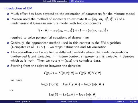
Introduction of EM

Much effort has been devoted to the estimation of parameters for the mixture model

Pearson used the method of moments to estimate θ = (m1, m2, s21 , s2

2 , π) of aunidimensional Gaussian mixture model with two components

f (x i ; θ) = πϕ(x i ;m1, s21 ) + (1 − π)ϕ(x i ; m2, s

22 )

required to solve polynomial equations of degree nine

Generally, the appropriate method used in this context is the EM algorithm(Dempster et al., 1977). Two steps Estimation and Maximization

This algorithm can be applied in different contexts where the model depends onunobserved latent variables. In mixture context z represents this variable. It denoteswhich x i is from. Then we note y = (x, z) the complete data.

Starting from the relation between the densities

f (y, θ) = f ((x, z); θ) = f (y|x; θ)f (x; θ)

we havelog(f (x; θ)) = log(f (y, θ)) − log(f (y|x; θ))

orLM(θ) = LC (z; θ) − log f (y|x; θ)



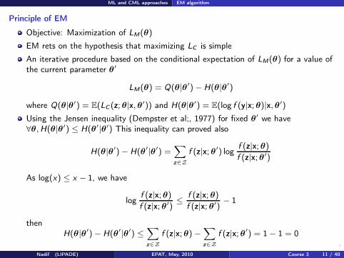
Principle of EM

Objective: Maximization of LM(θ)

EM rets on the hypothesis that maximizing LC is simple

An iterative procedure based on the conditional expectation of LM(θ) for a value ofthe current parameter θ′

LM(θ) = Q(θ|θ′) − H(θ|θ′)

where Q(θ|θ′) = E(LC (z; θ|x, θ′)) and H(θ|θ′) = E(log f (y|x; θ)|x, θ′)

Using the Jensen inequality (Dempster et al;, 1977) for fixed θ′ we have∀θ, H(θ|θ′) ≤ H(θ′|θ′) This inequality can proved also

H(θ|θ′) − H(θ′|θ′) =∑

z∈Z

f (z|x; θ′) logf (z|x; θ)

f (z|x; θ′)

As log(x) ≤ x − 1, we have

logf (z|x; θ)

f (z|x; θ′)≤ f (z|x; θ)

f (z|x; θ′)− 1

thenH(θ|θ′) − H(θ′|θ′) ≤

∑

z∈Z

f (z|x; θ) −∑

z∈Z

f (z|x; θ′) = 1 − 1 = 0



Q(θ|θ′)

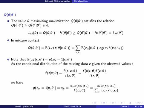
The value θ maximizing maximization Q(θ|θ′) satisfies the relationQ(θ|θ′) ≥ Q(θ′|θ′) and,

LM(θ) = Q(θ|θ′) − H(θ|θ′) ≥ Q(θ′|θ′) − H(θ′|θ′) = LM(θ′)

In mixture context

Q(θ|θ′) = E(LC (z; θ|x, θ′)) =∑

i,k

E(zik |x, θ′) log(πk f (x i ; αk))

Note that E(zik |x, θ′) = p(zik = 1|x, θ′)As the conditional distribution of the missing data z given the observed values :

f (z|x; θ) =f (x, z; θ)

f (x; θ)=

f (x|z; θ)f (z; θ)

f (x; θ)

we have

p(zik = 1|x, θ′) = sik =πkϕ(x i ; αk)

f (xi ; θ)=

πkϕ(x i ; αk)∑

` π`ϕ(x i ; α`)



The steps of EM

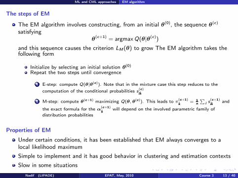
The EM algorithm involves constructing, from an initial θ(0), the sequence θ(c)

satisfyingθ

(c+1) = argmaxQ(θ|θ(c))

and this sequence causes the criterion LM(θ) to grow The EM algorithm takes thefollowing form

Initialize by selecting an initial solution θ(0)

Repeat the two steps until convergence

1 E-step: compute Q(θ|θ(c)). Note that in the mixture case this step reduces to the

computation of the conditional probabilities s(c)

ik

2 M-step: compute θ(c+1) maximizing Q(θ, θ(c)). This leads to π(c+1)

k= 1

n

∑

i s(c+1)

ikand

the exact formula for the α(c+1)

kwill depend on the involved parametric family of

distribution probabilities

Properties of EM

Under certain conditions, it has been established that EM always converges to alocal likelihood maximum

Simple to implement and it has good behavior in clustering and estimation contexts

Slow in some situations



An other interpretation of EM

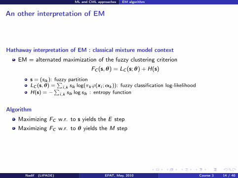
Hathaway interpretation of EM : classical mixture model context

EM = alternated maximization of the fuzzy clustering criterion

FC (s, θ) = LC (s; θ) + H(s)

s = (sik ): fuzzy partitionLC (s, θ) =

∑

i,k sik log(πkϕ(x i ;αk )): fuzzy classification log-likelihood

H(s) = −∑

i,k sik log sik : entropy function

Algorithm

Maximizing FC w.r. to s yields the E step

Maximizing FC w.r. to θ yields the M step


ML and CML approaches CEM algorithm

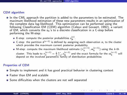
CEM algorithm

In the CML approach the partition is added to the parameters to be estimated. Themaximum likelihood estimation of these new parameters results in an optimization ofthe complete data log-likelihood. This optimization can be performed using thefollowing Classification EM (CEM) algorithm (Celeux and Govaert, 1992), a variantof EM, which converts the sik ’s to a discrete classification in a C-step beforeperforming the M-step:

E-step: compute the posterior probabilities s(c)ik

.

C-step: the partition z(c+1) is defined by assigning each observation x i to the cluster

which provides the maximum current posterior probability.

M-step: compute the maximum likelihood estimate (π(c+1)k

, α(c+1)k

) using the k-th

cluster. This leads to π(c+1)k

= 1n

∑

i z(c+1)ik

and the exact formula for the α(c+1)k

willdepend on the involved parametric family of distribution probabilities

Properties of CEM

Simple to implement and it has good practical behavior in clustering context

Faster than EM and scalable

Some difficulties when the clusters are not well separated


ML and CML approaches CEM algorithm

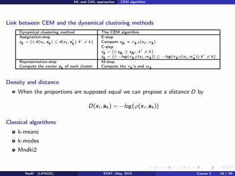
Link between CEM and the dynamical clustering methods

Dynamical clustering method The CEM algorithm

Assignation-step E-step

zk = {i ; d(x i , ak ) ≤ d(x i , a′

k); k′ 6= k} Compute sik ∝ πkϕ(x i , αk )

C-step

zk = {i ; sik ≥ sik′ ; k′ 6= k}

zk = {i ;−log(πkϕ(x i , αk )) ≤ −log(πkϕ(x i , α′

k)); k′ 6= k}

Representation-step M-stepCompute the center ak of each cluster Compute the πk ’s and αk

Density and distance

When the proportions are supposed equal we can propose a distance D by

D(x i , ak) = −log(ϕ(x i , ak))

Classical algorithms

k-means

k-modes

Mndki2


ML and CML approaches Others variants of EM

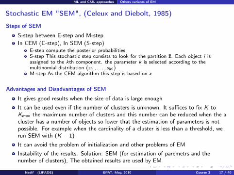
Stochastic EM "SEM", (Celeux and Diebolt, 1985)

Steps of SEM

S-step between E-step and M-step

In CEM (C-step), In SEM (S-step)E-step compute the posterior probabilitiesS-step This stochastic step consists to look for the partition z̄. Each object i isassigned to the kth component. the parameter k is selected according to themultinomial distribution (si1, . . . , siK )M-step As the CEM algorithm this step is based on z̄

Advantages and Disadvantages of SEM

It gives good results when the size of data is large enough

It can be used even if the number of clusters is unknown. It suffices to fix K toKmax the maximum number of clusters and this number can be reduced when the acluster has a number of objects so lower that the estimation of parameters is notpossible. For example when the cardinality of a cluster is less than a threshold, werun SEM with (K − 1)

It can avoid the problem of initialization and other problems of EM

Instability of the results. Solution: SEM (for estimation of paremetrs and thenumber of clusters), The obtained results are used by EM


ML and CML approaches Others variants of EM

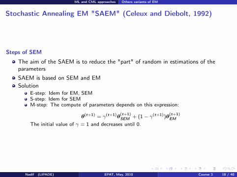
Stochastic Annealing EM "SAEM" (Celeux and Diebolt, 1992)

Steps of SEM

The aim of the SAEM is to reduce the "part" of random in estimations of theparameters

SAEM is based on SEM and EM

SolutionE-step: Idem for EM, SEMS-step: Idem for SEMM-step: The compute of parameters depends on this expression:

θ(t+1) = γ(t+1)θ(t+1)SEM

+ (1 − γ(t+1))θ(t+1)EM

The initial value of γ = 1 and decreases until 0.


Applications

Outline

1 Introduction

Mixture Approach





4 Applications


5 Model Selection

6 Conclusion


Applications Gaussian mixture model

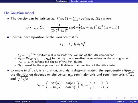
The Gaussian model

The density can be written as: f (x i ; θ) =∑

k πkϕ(x i ; µk , Σk) where

ϕ(x i ; µk , Σk ) =1

(2π)p2 |Σk |

1

2

exp{−1

2(x i − µk)

TΣ−1k (x i − µk)}

Spectral decomposition of the variance matrix

Σk = λkDkAkDTk

- λk = |Σk |1/p positive real represents the volume of the kth component

- Ak = Diag(ak1, . . . , akp) formed by the normalized eigenvalues in decreasing order|Ak | = 1. It defines the shape of the kth cluster

- Dk formed by the eigenvectors. It defines the direction of the kth cluster

Example in R2, Dk is a rotation, and Ak is diagonal matrix, the equidensity ellipse of

the distribution depends on the center µk , semimajor axis and semiminor axis√

λka

and√

λk/a

Dk =

(

cos(α) sin(α)−sin(α) cos(α)

)

Ak =

(

a 00 1/a

)



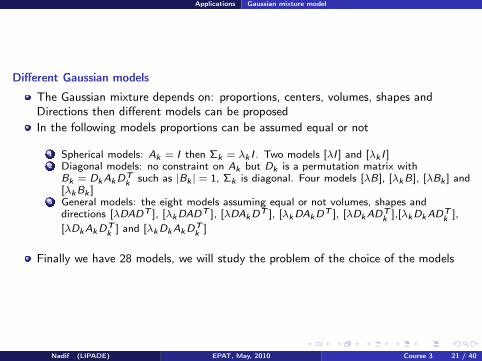
Different Gaussian models

The Gaussian mixture depends on: proportions, centers, volumes, shapes andDirections then different models can be proposed

In the following models proportions can be assumed equal or not

1 Spherical models: Ak = I then Σk = λk I . Two models [λI ] and [λk I ]2 Diagonal models: no constraint on Ak but Dk is a permutation matrix with

Bk = DkAkDTk

such as |Bk | = 1, Σk is diagonal. Four models [λB], [λkB], [λBk ] and[λkBk ]

3 General models: the eight models assuming equal or not volumes, shapes anddirections [λDADT ], [λkDADT ], [λDAkDT ], [λkDAkDT ], [λDkADT

k],[λkDkADT

k],

[λDkAkDTk

] and [λkDkAkDTk

]

Finally we have 28 models, we will study the problem of the choice of the models



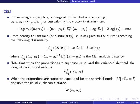
CEM

In clustering step, each x i is assigned to the cluster maximizingsik ∝ πkϕ(x i ; µk , Σk) or equivalently the cluster that minimizes

− log(πkϕ(x i ; αk)) = (x i − µk)TΣ−1

k (x i − µk) + log |Σk | − 2 log(πk) + cste

From density to Distance (or dissimilarity), x i is assigned to the cluster accordingthe following dissimilarity

dΣ−1

k(x i ; µk) + log |Σk | − 2 log(πk)

where dΣ−1

k(x i ; µk) = (x i − µk)

T Σ−1k (x i − µk) is the Mahanalobis distance

Note that when the proportions are supposed equal and the variances identical, theassignation is based only on

d2

Σ−1

k

(x i ; µk)

When the proportions are supposed equal and for the spherical model [λI ] (Σk = I ),one uses the usual euclidean distance

d2(x i ; µk)



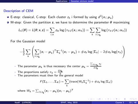
Description of CEM

E-step: classical, C-step: Each cluster zk i formed by using d2(x i ; µk)

M-step: Given the partition z, we have to determine the parameter θ maximizing

LC (θ) = L(θ; x, z) =∑

i,k

zik log (πkϕ(x i ; αk)) =∑

k

∑

i∈zk

log (πkϕ(x i ; αk))

For the Gaussian model

−1

2

∑

k

∑

i∈zk

(x i − µk)TΣ−1k (x i − µk) + #zk log |Σk | − 2#zk log(πk)

- The parameter µk is thus necessary the center µk =

∑

i∈zk

x i

#zk

- The proportions satisfy πk =#zkn

- The parameters must then for the general model

F (Σ1, . . . , ΣK ) =∑

k

(trace(WkΣ−1k

) + #zk log |Σk |)

where Wk =∑

i∈zk(x i − µk)(x i − µk )T



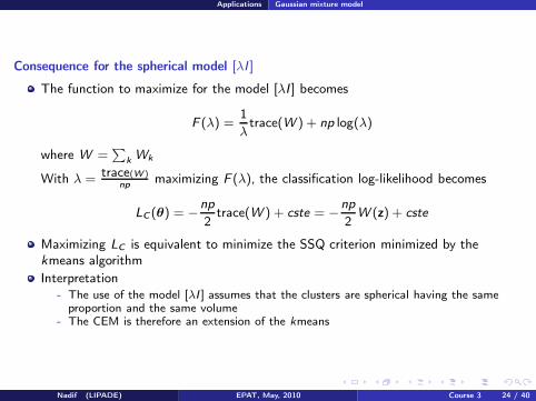
Consequence for the spherical model [λI ]

The function to maximize for the model [λI ] becomes

F (λ) =1

λtrace(W ) + np log(λ)

where W =∑

k Wk

With λ = trace(W )np

maximizing F (λ), the classification log-likelihood becomes

LC (θ) = −np

2trace(W ) + cste = −np

2W (z) + cste

Maximizing LC is equivalent to minimize the SSQ criterion minimized by thekmeans algorithm

Interpretation- The use of the model [λI ] assumes that the clusters are spherical having the same

proportion and the same volume- The CEM is therefore an extension of the kmeans



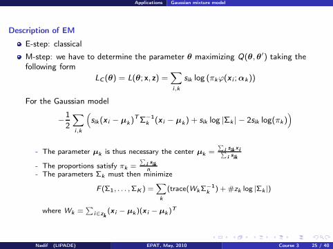
Description of EM

E-step: classical

M-step: we have to determine the parameter θ maximizing Q(θ, θ′) taking thefollowing form

LC (θ) = L(θ; x, z) =∑

i,k

sik log (πkϕ(x i ; αk))

For the Gaussian model

−1

2

∑

i,k

(

sik(x i − µk)TΣ−1k (x i − µk) + sik log |Σk | − 2sik log(πk)

)

- The parameter µk is thus necessary the center µk =∑

i sik x i∑

i sik

- The proportions satisfy πk =∑

i sikn

- The parameters Σk must then minimize

F (Σ1, . . . , ΣK ) =∑

k

(trace(WkΣ−1k

) + #zk log |Σk |)

where Wk =∑

i∈zk(x i − µk)(x i − µk )T


Applications Bernoulli mixture

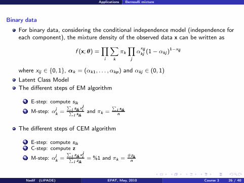
Binary data

For binary data, considering the conditional independence model (independence foreach component), the mixture density of the observed data x can be written as

f (x; θ) =∏

i

∑

k

πk

∏

j

αxij

kj (1 − αkj )1−xij

where xij ∈ {0, 1}, αk = (αk1, . . . , αkp) and αkj ∈ (0, 1)

Latent Class Model

The different steps of EM algorithm

1 E-step: compute sik

2 M-step: αjk

=∑

i sik xji

∑

i sikand πk =

∑

i sikn

The different steps of CEM algorithm

1 E-step: compute sik2 C-step: compute z

3 M-step: αjk

=∑

i zik xji

∑

i zik= %1 and πk =

#zkn



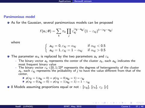
Parsimonious model

As for the Gaussian, several parsimonious models can be proposed

f (xi ; θ) =∑

k

πk

∏

j

ε|xij−akj |

kj (1 − εkj )1−|xij−akj |

where{

akj = 0, εkj = αkj if αkj < 0.5akj = 1, εkj = 1 − αkj if αkj > 0.5

The parameter αk is replaced by the two parameters ak and εk

- The binary vector ak represents the center of the cluster zk , each akj indicates themost frequent binary value

- The binary vector εk ∈]0, 1/2[p represents the degrees of heterogeneity of the clusterzk , each εkj represents the probability of j to have the value different from that of thecenter,

p(xij = 1|akj = 0) = p(xij = 0|akj = 1) = εkj

p(xij = 0|akj = 0) = p(xij = 1|akj = 1) = 1 − εkj

8 Models assuming proportions equal or not : [εkj ], [εk ], εj , [ε]



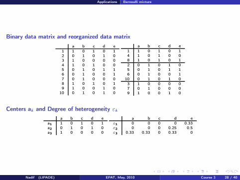
Binary data matrix and reorganized data matrix

a b c d e

1 1 0 1 0 12 0 1 0 1 03 1 0 0 0 04 1 0 1 0 05 0 1 0 1 16 0 1 0 0 1

7 0 1 0 0 08 1 0 1 0 19 1 0 0 1 0

10 0 1 0 1 0

a b c d e

1 1 0 1 0 14 1 0 1 0 08 1 0 1 0 1

2 0 1 0 1 05 0 1 0 1 16 0 1 0 0 1

10 0 1 0 1 0

3 1 0 0 0 07 0 1 0 0 09 1 0 0 1 0

Centers ak and Degree of heterogeneity εk

a b c d e

a1 1 0 1 0 1a2 0 1 0 1 0a3 1 0 0 0 0

a b c d e

ε1 0 0 0 0 0.33ε2 0 0 0 0.25 0.5ε3 0.33 0.33 0 0.33 0



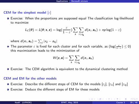
CEM for the simplest model [ε]

Exercise: When the proportions are supposed equal The classification log-likelihoodto maximize

LC (θ) = L(θ; x, z) = log(ε

1 − ε)∑

k

∑

i∈zk

d(x i , ak) + np log(1 − ε)

where d(x i , ak) =∑

j |xij − akj |The parameter ε is fixed for each cluster and for each variable, as (log( ε

1−ε) ≤ 0)

this maximization leads to the minimization of

W (z, a) =∑

k

∑

i∈zk

d(x i , ak)

Exercise: The CEM algorithm is equivalent to the dynamical clustering method

CEM and EM for the other models

Exercise: Describe the different steps of CEM for the models [εj ], [εk ] and [εkj ]

Exercise: Deduce the different steps of EM for these models


Applications Multinomial Mixture

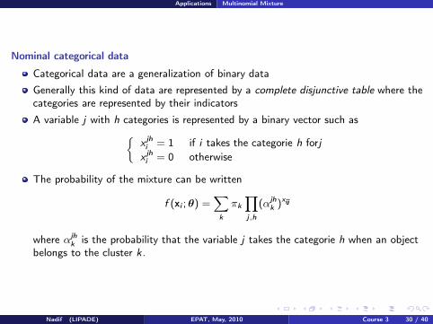
Nominal categorical data

Categorical data are a generalization of binary data

Generally this kind of data are represented by a complete disjunctive table where thecategories are represented by their indicators

A variable j with h categories is represented by a binary vector such as

{

xjhi = 1 if i takes the categorie h forj

xjhi = 0 otherwise

The probability of the mixture can be written

f (xi ; θ) =∑

k

πk

∏

j,h

(αjhk )xij

where αjhk is the probability that the variable j takes the categorie h when an object

belongs to the cluster k .



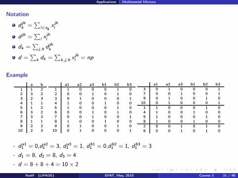
Notation

d jhk =

∑

i∈zkx jhi

d jh =∑

i xjhi

dk =∑

j,h djh

k

d =∑

k dk =∑

k,j,h xjhi = np

Example

a b

1 1 22 3 23 2 3

4 1 15 1 26 3 27 3 38 1 19 2 2

10 2 3

a1 a2 a3 b1 b2 b3

1 1 0 0 0 1 02 0 0 1 0 1 03 0 1 0 0 0 1

4 1 0 0 1 0 05 1 0 0 0 1 06 0 0 1 0 1 07 0 0 1 0 0 18 1 0 0 1 0 09 0 1 0 0 1 0

10 0 1 0 0 0 1

a1 a2 a3 b1 b2 b3

3 0 1 0 0 0 17 0 0 1 0 0 19 0 1 0 0 1 0

10 0 1 0 0 0 1

1 1 0 0 0 1 04 1 0 0 1 0 05 1 0 0 0 1 08 1 0 0 1 0 0

2 0 0 1 0 1 0

6 0 0 1 0 1 0

- da11 = 0,da2

1 = 3, da31 = 1, db1

1 = 0,db21 = 1, db3

1 = 3

- d1 = 8, d2 = 8, d3 = 4

- d = 8 + 8 + 4 = 10 × 2



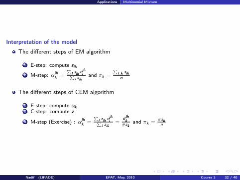
Interpretation of the model

The different steps of EM algorithm

1 E-step: compute sik

2 M-step: αjhk

=∑

i sik xjhi

∑

i sikand πk =

∑

i,k sikn

The different steps of CEM algorithm

1 E-step: compute sik2 C-step: compute z

3 M-step (Exercise) : αjhk

=∑

i zik xjhi

∑

i zik=

djhk

#zkand πk =

#zkn



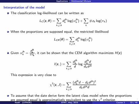
Interpretation of the model

The classification log-likelihood can be written as

LC (z, θ) =∑

k,j,h

djh

k log(αjh

k ) +∑

k

#zk log(πk)

When the proportions are supposed equal, the restricted likelihood

LCR(θ) =∑

k,j,h

djh

k log(αjh

k )

Given αjh

k =djhk

#zk, it can be shown that the CEM algorithm maximizes H(z)

I (z, ) =∑

k,j,h

djh

k

dlog

djh

k d

dkd jh

This expression is very close to

χ2(z, J) =∑

k,j,h

(d jh

k d − dkdjh)2

dkd jhd

To assume that the date derive form the latent class model where the proportionsare assumed equal is approximatively equivalent to use the χ2 criterion



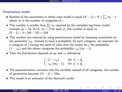
Parsimonious model

Number of the parameters in latent class model is equal (K − 1) + K ∗∑j mj − 1where mj is the number of categories of j

This number is smaller than∏

j mj required by the complete log-linear model,example (p = 10, K=5, mj = 4 for each j), this number is equal to(5 − 1) + 5 ∗ (40 − 10) = 154

This number can reduced by using parsimonious model by imposing constraints onthe paremetre αkj . Instead to have a probability for each categorie, we associate fora categorie of j having the same of value that the center for j the probability(1 − εkj ) and the others categories the probability εkj/(mj − 1)

Then the distribution depends on ak and εk defined by

{

(1 − εkj ) for xji = a

j

k

εkj/(mj − 1) for x ji 6= aj

k

The parametrization concerns only the variables instead of all categories, the numberof parameters becomes (K − 1) + 2Kp

This model is an extension of the Bernoulli model



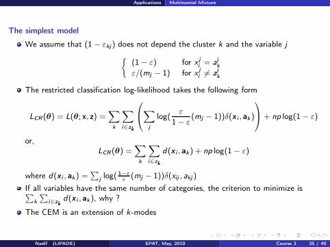
The simplest model

We assume that (1 − εkj ) does not depend the cluster k and the variable j

{

(1 − ε) for x ji = aj

k

ε/(mj − 1) for xji 6= a

j

k

The restricted classification log-likelihood takes the following form

LCR(θ) = L(θ; x, z) =∑

k

∑

i∈zk

∑

j

log(ε

1 − ε(mj − 1))δ(x i , ak)

+ np log(1 − ε)

or,LCR(θ) =

∑

k

∑

i∈zk

d(x i , ak) + np log(1 − ε)

where d(x i , ak) =∑

j log( 1−εε

(mj − 1))δ(xij , akj )

If all variables have the same number of categories, the criterion to minimize is∑

k

∑

i∈zkd(x i , ak), why ?

The CEM is an extension of k-modes



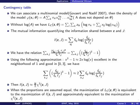
Contingency table

We can associate a multinomial model(Govaert and Nadif 2007), then the density ofthe model ϕ(xi ; θ) = A

∑

k πkαxi1k1 . . . α

xip

kp ( A does not depend on θ)

Without log(A) we have LC (z, θ) =∑

i

∑

k zik

(

log πk +∑

j xij log(αkj ))

The mutual information quantifying the information shared between z and J:

I (z, J) =∑

kj

fkj log(fkj

fk.f.j)

We have the relation∑

k,j

(fkj−fk.

f.j )

2

fk.

f.j

=∑

k,j

(

(fkj

fk.

f.j

)2 − 1)

Using the following approximation : x2 − 1 ≈ 2x log(x) excellent in theneighborhood of 1 and good in [0, 3], we have

∑

k,j

(

(fkj

fk.f.j)2 − 1

)

≈ 2∑

k,j

fkj log(fkj

fk.f.j)

Then I (z, J) ≈ N2χ2(z, J)

When the proportions are assumed equal, the maximization of LC (z, θ) is equivalentto the maximization of I (z, J) and approximately equivalent to the maximzation ofχ2(z, J)


Model Selection

Outline

1 Introduction

Mixture Approach





4 Applications


5 Model Selection

6 Conclusion


Model Selection

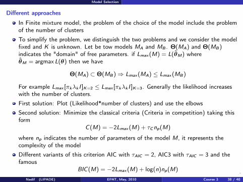
Different approaches

In Finite mixture model, the problem of the choice of the model include the problemof the number of clusters

To simplify the problem, we distinguish the two problems and we consider the modelfixed and K is unknown. Let be tow models MA and MB . Θ(MA) and Θ(MB)indicates the "domain" of free parameters. if Lmax(M) = L(θ̂M) whereθ̂M = argmaxL(θ) then we have

Θ(MA) ⊂ Θ(MB) ⇒ Lmax(MA) ≤ Lmax (MB)

For example Lmax [πkλk I ]K=2 ≤ Lmax [πkλk I ]K=3. Generally the likelihood increaseswith the number of clusters.

First solution: Plot (Likelihood*number of clusters) and use the elbows

Second solution: Minimize the classical criteria (Criteria in competition) taking thisform

C (M) = −2Lmax (M) + τCnp(M)

where np indicates the number of parameters of the model M, it represents thecomplexity of the model

Different variants of this criterion AIC with τAIC = 2, AIC3 with τAIC = 3 and thefamous

BIC(M) = −2Lmax (M) + log(n)np(M)


Conclusion

Outline

1 Introduction

Mixture Approach





4 Applications


5 Model Selection

6 Conclusion


Conclusion

Conclusion

Finite mixture approach is interesting

The CML approach gives interesting criteria and generalizes the classical criteria

The different variants of EM offer good solutions

The CEM algorithm is an extension of k-means and other variants

The choice of the model is performed by using the maximum likelihood penalized bythe number of parameters

See MIXMOD

Other Mixture models adapted to the nature of data (Text mining)


Documents

Finite Mixture Models and Clustering - College of … · Finite Mixture Models and Clustering Mohamed Nadif LIPADE, Université Paris Descartes, France Nadif (LIPADE) EPAT, May, 2010