Embed Size (px)
Citation preview

http://www.econometricsociety.org/
Econometrica, Vol. 77, No. 1 (January, 2009), 135–175
NONPARAMETRIC IDENTIFICATION OF FINITE MIXTUREMODELS OF DYNAMIC DISCRETE CHOICES
HIROYUKI KASAHARAUniversity of Western Ontario, London, Ontario N6A 5C2, Canada
KATSUMI SHIMOTSUQueen’s University, Kingston, Ontario, K7L 3N6 Canada
The copyright to this Article is held by the Econometric Society. It may be downloaded,printed and reproduced only for educational or research purposes, including use in coursepacks. No downloading or copying may be done for any commercial purpose without theexplicit permission of the Econometric Society. For such commercial purposes contactthe Office of the Econometric Society (contact information may be found at the websitehttp://www.econometricsociety.org or in the back cover of Econometrica). This statement mustthe included on all copies of this Article that are made available electronically or in any otherformat.
Econometrica, Vol. 77, No. 1 (January, 2009), 135–175
NONPARAMETRIC IDENTIFICATION OF FINITE MIXTUREMODELS OF DYNAMIC DISCRETE CHOICES
BY HIROYUKI KASAHARA AND KATSUMI SHIMOTSU1
In dynamic discrete choice analysis, controlling for unobserved heterogeneity is animportant issue, and finite mixture models provide flexible ways to account for it. Thispaper studies nonparametric identifiability of type probabilities and type-specific com-ponent distributions in finite mixture models of dynamic discrete choices. We derivesufficient conditions for nonparametric identification for various finite mixture mod-els of dynamic discrete choices used in applied work under different assumptions onthe Markov property, stationarity, and type-invariance in the transition process. Threeelements emerge as the important determinants of identification: the time-dimensionof panel data, the number of values the covariates can take, and the heterogeneity ofthe response of different types to changes in the covariates. For example, in a simplecase where the transition function is type-invariant, a time-dimension of T = 3 is suf-ficient for identification, provided that the number of values the covariates can take isno smaller than the number of types and that the changes in the covariates induce suffi-ciently heterogeneous variations in the choice probabilities across types. Identificationis achieved even when state dependence is present if a model is stationary first-orderMarkovian and the panel has a moderate time-dimension (T ≥ 6).
KEYWORDS: Dynamic discrete choice models, finite mixture, nonparametric identi-fication, panel data, unobserved heterogeneity.
1. INTRODUCTION
IN DYNAMIC DISCRETE CHOICE ANALYSIS, controlling for unobserved hetero-geneity is an important issue. Finite mixture models, which are commonly usedin empirical analyses, provide flexible ways to account for it. To date, however,the conditions under which finite mixture dynamic discrete choice models arenonparametrically identified are not well understood. This paper studies non-parametric identifiability of finite mixture models of dynamic discrete choiceswhen a researcher has access to panel data.
Finite mixtures have been used in numerous applications, especially in es-timating dynamic models. In empirical industrial organization, Crawford andShum (2005) used finite mixtures to control for patient-level unobserved het-erogeneity in estimating a dynamic matching model of pharmaceutical de-mand. Gowrisankaran, Mitchell, and Moro (2005) estimated a dynamic modelof voter behavior with finite mixtures. In labor economics, finite mixtures area popular choice for controlling for unobserved person-specific effects when
1The authors are grateful to the co-editor and three anonymous referees whose commentsgreatly improved the paper. The authors thank Victor Aguirregabiria, David Byrne, Seung HyunHong, Hidehiko Ichimura, Thierry Magnac, and the seminar participants at Hitotsubashi Uni-versity, University of Tokyo, University of Toronto, New York Camp Econometrics II, and 2006JEA Spring Meeting for helpful comments. The financial support from SSHRC is gratefully ac-knowledged.
© 2009 The Econometric Society DOI: 10.3982/ECTA6763
136 H. KASAHARA AND K. SHIMOTSU
dynamic discrete choice models are estimated (e.g., Keane and Wolpin (1997),Cameron and Heckman (1998)). Heckman and Singer (1984) used finite mix-tures to approximate more general mixture models in the context of durationmodels with unobserved heterogeneity.
In most applications of finite mixture models, the components of the mixturedistribution are assumed to belong to a parametric family. The nonparamet-ric maximum likelihood estimator (NPMLE) of Heckman and Singer (1984)treats the distribution of unobservables nonparametrically but assumes para-metric component distributions. Most existing theoretical work on identifica-tion of finite mixture models either treats component distributions parametri-cally or uses training data that are from known component distributions (e.g.,Titterington, Smith, and Makov (1985), Rao (1992)). As Hall and Zhou (2003)stated, “very little is known of the potential for consistent nonparametric in-ference in mixtures without training data.”
This paper studies nonparametric identifiability of type probabilities andtype-specific component distributions in finite mixture dynamic discrete choicemodels. Specifically, we assess the identifiability of type probabilities and type-specific component distributions when no parametric assumption is imposedon them. Our point of departure is the work of Hall and Zhou (2003), whoproved nonparametric identifiability of two-type mixture models with indepen-dent marginals:
F(y)= π
T∏t=1
F 1t (yt)+ (1 −π)
T∏t=1
F 2t (yt)�(1)
where F(y) is the distribution function of a T -dimensional variable Y , andF
jt (yt) is the distribution function of the tth element of Y conditional on type j.
Hall and Zhou showed that the type probability π and the type-specific compo-nents Fj
t are nonparametrically identifiable from F(y) and its marginals whenT ≥ 3, while they are not when T = 2. The intuition behind their result is as fol-lows. Integrating out different elements of y from (1) gives lower-dimensionalsubmodels,
F(yi1� yi2� � � � � yil
) = π
l∏s=1
F 1is
(yis
) + (1 −π)
l∏s=1
F 2is
(yis
)�(2)
where 1 ≤ l ≤ T , 1 ≤ i1 < · · · < il ≤ T , and F(yi1� yi2� � � � � yil ) is the l-variatemarginal distribution of F(y). Each lower-dimensional submodel implies a dif-ferent restriction on the unknown elements, that is, π and the F
jt ’s. F and
its marginals imply 2T − 1 restrictions, while there are 2T + 1 unknown ele-ments. When T = 3, the number of restrictions is the same as the number ofunknowns, and one can solve these restrictions to uniquely determine π andthe F
jt ’s.
MODELS OF DYNAMIC DISCRETE CHOICES 137
While Hall and Zhou’s analysis provides the insight that lower-dimensionalsubmodels (2) provide important restrictions for identification, it has limitedapplicability to the finite mixture models of dynamic discrete choices in eco-nomic applications. First, it is difficult to generalize their analysis to three ormore types.2 Second, their model (1) does not have any covariates, while mostempirical models in economics involve covariates. Third, the assumption thatelements of y are independent in (1) is not realistic in dynamic discrete choicemodels.
This paper provides sufficient conditions for nonparametric identificationfor various finite mixture models of dynamic discrete choices used in appliedwork. Three elements emerge as the important determinants of identification:the time-dimension of panel data, the number of the values the covariates cantake, and the heterogeneity of the response of different types to changes inthe covariates. For example, in a simple case where the transition function istype-invariant, a time-dimension of T = 3 is sufficient for identification, pro-vided that the number of values the covariates can take is no smaller than thenumber of types and that the changes in the covariates induce sufficiently het-erogeneous variations in the choice probabilities across types.
The key insight is that, in models with covariates, different sequences of co-variates imply different identifying restrictions in the lower-dimensional sub-models; in fact, if d is the number of support points of the covariates and Tis the time-dimension, then the number of restrictions becomes on the orderof dT . As a result, the presence of covariates provides a powerful source ofidentification in panel data even with a moderate time-dimension T .
We study a variety of finite mixture dynamic discrete choice models un-der different assumptions on the Markov property, stationarity, and type-invariance in the transition process. Under a type-invariant transition func-tion and conditional independence, we analyze the nonstationary case thatconditional choice probabilities change over time because time-specific aggre-gate shocks are present or agents are finitely lived. We also examine the casewhere state dependence is present (for instance, when the lagged choice af-fects the current choice and/or the transition function of state variables is dif-ferent across types), and show that identification is possible when a model isstationary first-order Markovian and the panel has a moderate time-dimensionT ≥ 6. This result is important since distinguishing unobserved heterogeneityand state dependence often motivates the use of finite mixture models in em-pirical studies. On the other hand, our approach has a limitation in that it doesnot simultaneously allow for both state dependence and nonstationarity.
2When the number of types, M , is more than three, Hall, Neeman, Pakyari, and Elmore (2005)showed that for any number of types, M , there exists TM such that type probabilities and type-specific component distributions are nonparametrically identifiable when T ≥ TM , and that TM isno larger than (1 + o(1))6M ln(M) as M increases. However, such a TM is too large for typicalpanel data sets.
138 H. KASAHARA AND K. SHIMOTSU
We also study nonparametric identifiability of the number of types, M . Un-der the assumptions on the Markov property, stationarity, and type-invarianceused in this paper, we show that the lower bound of M is identifiable and, fur-thermore, M itself is identified if the changes in covariates provide sufficientvariation in the choice probabilities across types.
Nonparametric identification and estimation of finite mixture dynamic dis-crete choice models are relevant and useful in practical applications for, atleast, the following reasons. First, choosing a parametric family for the com-ponent distributions is often difficult because of a lack of guidance from eco-nomic theory; nonparametric estimation provides a flexible way to reveal thestructure hidden in the data. Furthermore, even when theory offers guidance,comparing parametric and nonparametric estimates allows us to examine thevalidity of the restrictions imposed by the underlying theoretical model.
Second, analyzing nonparametric identification helps us understand theidentification of parametric or semiparametric finite mixture models of dy-namic discrete choices. Understanding identification is not a simple task forfinite mixture models even with parametric component distributions, and for-mal identification analysis is rarely provided in empirical applications. Oncetype probabilities and component distributions are nonparametrically identi-fied, the identification analysis of parametric finite mixture models often be-comes transparent as it is reduced to the analysis of models without unobservedheterogeneity. As we demonstrate through examples, our nonparametric iden-tification results can be applied to check the identifiability of some parametricfinite mixture models.
Third, the identification results of this paper will open the door to apply-ing semiparametric estimators for structural dynamic models to models withunobserved heterogeneity. Recently, by building on the seminal work by Hotzand Miller (1993), computationally attractive semiparametric estimators forstructural dynamic models have been developed (Aguirregabiria and Mira(2002), Kasahara and Shimotsu (2008a)), and a number of papers in empiricalindustrial organization have proposed two-/multistep estimators for dynamicgames (e.g., Bajari, Benkard, and Levin (2007), Pakes, Ostrovsky, and Berry(2007), Pesendorfer and Schmidt-Dengler (2008), Bajari and Hong (2006), andAguirregabiria and Mira (2007)). To date, however, few of these semiparamet-ric estimators have been extended to accommodate unobserved heterogeneity.This is because these estimators often require an initial nonparametric con-sistent estimate of type-specific component distributions, but it has not beenknown whether one can obtain a consistent nonparametric estimate in finitemixture models.3 The identification results of this paper provide an apparatus
3It is believed that it is not possible to obtain a consistent estimate of choice probabilities.For instance, Aguirregabiria and Mira (2007) proposed a pseudo maximum likelihood estima-tion algorithm for models with unobserved heterogeneity, but stated that (p. 15) “for [modelswith unobservable market characteristics] it is not possible to obtain consistent nonparametric
MODELS OF DYNAMIC DISCRETE CHOICES 139
that enables researchers to apply these semiparametric estimators to the mod-els with unobserved heterogeneity. This is important since it is often crucial tocontrol for unobserved heterogeneity in dynamic models (see Aguirregabiriaand Mira (2007)).
In a closely related paper, Kitamura (2004) examined nonparametric iden-tifiability of finite mixture models with covariates. Our paper shares his in-sight that the variation in covariates may provide a source of identification;however, the setting as well as the issues we consider are different from Kita-mura’s. We study discrete choice models in a dynamic setting with panel data,while Kitamura considered regression models with continuous dependent vari-ables with cross-sectional data. We address various issues specific to dynamicdiscrete choice models, including identification in the presence of state depen-dence and type-dependent transition probabilities for endogenous explanatoryvariables.
Our work provides yet another angle for analysis that relates current andprevious work on dynamic discrete choice models. Honoré and Tamer (2006)studied identification of dynamic discrete choice models, including the initialconditions problem, and suggested methods to calculate the identified sets.Rust (1994), Magnac and Thesmar (2002), and Aguirregabiria (2006) studiedthe identification of structural dynamic discrete choice models. Our analysisis also related to an extensive literature on identification of duration models(e.g., Elbers and Ridder (1982), Heckman and Singer (1984), Ridder (1990),and Van den Berg (2001)).
The rest of the paper is organized as follows. Section 2 discusses our ap-proach to identification and provides the identification results using a simple“baseline” model. Section 3 extends the identification analysis of Section 2, andstudies a variety of finite mixture dynamic discrete choice models. Section 4concludes. The proofs are collected in the Appendix.
2. NONPARAMETRIC IDENTIFICATION OF FINITE MIXTURE MODELS OFDYNAMIC DISCRETE CHOICES
Every period, each individual makes a choice at from the discrete and finiteset A, conditioning on (xt� xt−1� at−1) ∈ X × X × A, where xt is observableindividual characteristics that may change over time and the lagged choice at−1
is included as one of the conditioning variables. Each individual belongs to oneof M types, and his/her type attribute is unknown. The probability of belongingto type m is πm, where the πm’s are positive and sum to 1.
Throughout this paper, we impose a first-order Markov property on the con-ditional choice probability of at and denote type m’s conditional choice prob-ability by Pm(at |xt�xt−1� at−1). The initial distribution of (x1� a1) and the tran-sition probability function of xt are also different across types. For each type
estimates of [choice probabilities].” Furthermore, Geweke and Keane (2001, p. 3490) wrote that“the [Hotz and Miller] methods cannot accommodate unobserved state variables.”
140 H. KASAHARA AND K. SHIMOTSU
m, we denote them by p∗m(x1� a1) and fmt (xt |{xτ�aτ}t−1
τ=1), respectively. With aslight abuse of notation, we let p∗m(x1� a1) and fm
t (xt |{xτ�aτ}t−1τ=1) denote the
density of the continuously distributed elements of xt and the probability massfunction of the discretely distributed elements of xt .
Suppose we have a panel data set with time-dimension equal to T . Eachindividual observation, wi = {ait� xit}Tt=1, is drawn randomly from an M-termmixture distribution,
P({at�xt}Tt=1)(3)
=M∑
m=1
πmp∗m(x1� a1)
T∏t=2
fmt (xt |{xτ�aτ}t−1
τ=1)Pmt (at |xt� {xτ�aτ}t−1
τ=1)
=M∑
m=1
πmp∗m(x1� a1)
T∏t=2
fmt (xt |{xτ�aτ}t−1
τ=1)Pmt (at |xt�xt−1� at−1)�
where the first equality presents a general mixture model, while the secondequality imposes the Markovian assumption on the conditional choice proba-bilities, Pm
t (at |xt� {xτ�aτ}t−1τ=1) = Pm
t (at |xt�xt−1� at−1). This is the key identifyingassumption of this paper. The left-hand side of (3) is the distribution functionof the observable data, while the right-hand side of the second equality con-tains the objects we would like the data to inform us about.
REMARK 1: In models where at and xt follow a stationary first-order Markovprocess, it is sometimes assumed that the choice of the distribution of the initialobservation, p∗m(x1� a1), is the stationary distribution that satisfies the fixedpoint constraint
p∗m(x1� a1)=∑x′∈X
∑a′∈A
Pm(a1|x1�x′� a′)fm(x1|x′� a′)p∗m(x′� a′)�(4)
when all the components of x have finite support. When x is continuously dis-tributed, we replace the summation over x′ with integration. Our identificationresult does not rely on the stationarity assumption of the initial conditions.
The model (3) includes the following examples as special cases.
EXAMPLE 1—Dynamic Discrete Choice Model With Heterogeneous Coef-ficients: Denote a parameter vector specific to type m’s individual by θm =(βm′�ρm)′. Consider a dynamic binary choice model for individual i who be-longs to type m:
Pm(ait = 1|xit� {xiτ� aiτ}t−1τ=1) = Pm(ait = 1|xit� ai�t−1)(5)
= Φ(x′itβ
m + ρmai�t−1)�
MODELS OF DYNAMIC DISCRETE CHOICES 141
where the first equality imposes the Markovian assumption and the secondfollows from the parametric restriction with Φ(·) denoting the standard normalcumulative distribution function (c.d.f.). The distribution of xit conditional on(xi�t−1� ai�t−1) is specific to the value of θm. Since the evolution of (xit� ait) inthe presample period is not independent of random coefficient θm, the initialdistribution of (xi1� ai1) depends on the value of θm (cf. Heckman (1981)).
Browning and Carro (2007) estimated a continuous mixture version of (5)for the purchase of milk using a Danish consumer “long” panel (T ≥ 100),and provided evidence for heterogeneity in coefficients. Their study illustratesthat allowing for such heterogeneity can make a significant difference for out-comes of interest such as the marginal dynamic effect. In practice however,researchers quite often only have access to a short panel. The results of thispaper are therefore useful to understand the extent to which unobserved het-erogeneity in coefficients is identified in such a situation.
Our identification results are not applicable, however, to a parametric dy-namic discrete choice model with serially correlated idiosyncratic shocks; forexample, ait = 1(x′
itβm + ρmai�t−1 + εit), where εit is serially correlated.
EXAMPLE 2—Structural Dynamic Discrete Choice Models: Type m’s agentmaximizes the expected discounted sum of utilities, E[∑∞
j=0 βj{u(xt+j� at+j;
θm)+ εt+j(at+j)}|at�xt;θm], where xt is an observable state variable and εt(at)is a state variable that are known to the agent but not to the researcher. TheBellman equation for this dynamic optimization problem is
V (x) =∫
maxa∈A
{u(x�a;θm)+ ε(a)+β
∑x′∈X
V (x′)f (x′|x�a;θm)
}(6)
× g(dε|x)�where g(ε|x) is the joint distribution of ε = {ε(j) : j ∈ A} and f (x′|x�a;θm) isa type-specific transition function. The conditional choice probability is
Pθm(a|x) =∫
1{a = arg max
j∈A
[u(x� j;θm)+ ε(j)(7)
+β∑x′∈X
Vθm(x′)f (x′|x� j;θm)
]}
× g(dε|x)�where Vθm is the fixed point of (6). Let Pm
t (at |xt�xt−1� at−1) = Pθm(at |xt)and fm
t (xt |{xτ�aτ}t−1τ=1) = f (xt |xt−1� at−1;θm) in (3). The initial distribution of
(x1� a1) is given by the stationary distribution (4). Then the likelihood functionfor {at�xt}Tt=1 is given by (3) with (4).
142 H. KASAHARA AND K. SHIMOTSU
We study the nonparametric identifiability of the type probabilities, theinitial distribution, the type-specific conditional choice probabilities, and thetype-specific transition function in equation (3), which we denote by θ ={πm�p∗m(·)� {Pm
t (·|·)� fmt (·|·)}Tt=2}Mm=1. Following the standard definition of non-
parametric identifiability, θ is said to be nonparametrically identified (or iden-tifiable) if it is uniquely determined by the distribution function P({at�xt}Tt=1),without making any parametric assumption about the elements of θ. Becausethe order of the component distributions can be changed, θ is identified onlyup to a permutation of the components. If no two of the π’s are identical, wemay uniquely determine the components by assuming π1 <π2 < · · ·<πM .
2.1. Our Approach and Identification of the Baseline Model
The finite mixture models studied by Hall and Zhou (2003) have no covari-ates as discussed in the Introduction. In this subsection, we show that the pres-ence of covariates in our model creates a powerful source of identification.
First, we impose the following simplifying assumptions on the general model(3) and analyze the nonparametric identifiability of the resulting “baselinemodel.” Analyzing the baseline model helps elucidate the basic idea of ourapproach and clarifies the logic behind our main results. In the subsequentsections, we relax Assumption 1 in various ways and study how it affects theidentifiability of the resulting models.
ASSUMPTION 1: (a) The choice probability of at does not depend on time.(b) The choice probability of at is independent of the lagged variable (xt−1� at−1)conditional on xt . (c) fm
t (xt |{xτ�aτ}t−1τ=1) > 0 for all (xt� {xτ�aτ}t−1
τ=1) ∈ Xt ×At−1 and for all m. (d) The transition function is common across types;fmt (xt |{xτ�aτ}t−1
τ=1) = ft(xt |{xτ�aτ}t−1τ=1) for all m. (e) The transition function is
stationary; ft(xt |{xτ�aτ}t−1τ=1)= f (xt |xt−1� at−1) for all m.
Under Assumptions 1(a) and (b), the choice probabilities are written asPmt (at |xt�xt−1� at−1) = Pm(at |xt), where at−1 is not one of the elements of xt .
Under Assumption 1(b), the lagged variable (xt−1� at−1) affects the currentchoice at only through its effect on xt via fm
t (xt |{xτ�aτ}t−1τ=1). Assumption 1(c)
implies that, starting from any combinations of the past state and action, anystate x′ ∈X is reached in the next period with positive probability.
With Assumption 1 imposed, the baseline model is
P({at�xt}Tt=1)=M∑
m=1
πmp∗m(x1� a1)
T∏t=2
f (xt |xt−1� at−1)Pm(at |xt)�(8)
Since f (xt |xt−1� at−1) is nonparametrically identified directly from the observeddata (cf. Rust (1987)), we may assume f (xt |xt−1� at−1) is known without af-fecting the other parts of the argument. Divide P({at�xt}Tt=1) by the transition
MODELS OF DYNAMIC DISCRETE CHOICES 143
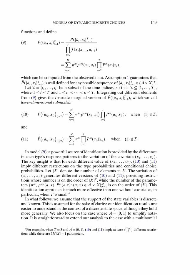
functions and define
P({at�xt}Tt=1) = P({at�xt}Tt=1)T∏t=2
f (xt |xt−1� at−1)
(9)
=M∑
m=1
πmp∗m(x1� a1)
T∏t=2
Pm(at |xt)�
which can be computed from the observed data. Assumption 1 guarantees thatP({at�xt}Tt=1) is well defined for any possible sequence of {at�xt}Tt=1 ∈ (A×X)T .
Let I = {i1� � � � � il} be a subset of the time indices, so that I ⊆ {1� � � � �T },where 1 ≤ l ≤ T and 1 ≤ i1 < · · · < il ≤ T . Integrating out different elementsfrom (9) gives the l-variate marginal version of P({at�xt}Tt=1), which we calllower-dimensional submodels
P({ais � xis
}is∈I
) =M∑
m=1
πmp∗m(x1� a1
) l∏s=2
Pm(ais |xis )� when {1} ∈ I�(10)
and
P({ais � xis
}is∈I
) =M∑
m=1
πm
l∏s=1
Pm(ais |xis
)� when {1} /∈ I�(11)
In model (9), a powerful source of identification is provided by the differencein each type’s response patterns to the variation of the covariate (x1� � � � � xT ).The key insight is that for each different value of (x1� � � � � xT ), (10) and (11)imply different restrictions on the type probabilities and conditional choiceprobabilities. Let |X| denote the number of elements in X . The variation of(x1� � � � � xT ) generates different versions of (10) and (11), providing restric-tions whose number is on the order of |X|T , while the number of the parame-ters {πm�p∗m(a�x)�Pm(a|x) : (a�x) ∈ A × X}Mm=1 is on the order of |X|. Thisidentification approach is much more effective than one without covariates, inparticular, when T is small.4
In what follows, we assume that the support of the state variables is discreteand known. This is assumed for the sake of clarity: our identification results areeasier to understand in the context of a discrete state space, although they holdmore generally. We also focus on the case where A = {0�1} to simplify nota-tion. It is straightforward to extend our analysis to the case with a multinomial
4For example, when T = 3 and A = {0�1}, (10) and (11) imply at least(|X|+2
3
)different restric-
tions while there are 3M|X| − 1 parameters.

144 H. KASAHARA AND K. SHIMOTSU
choice of a, but with heavier notation. Note also that Chandra (1977) showsthat a multivariate finite mixture model is identified if all the marginal modelsare identified.
It is convenient to collect notation first. Define, for ξ ∈ X ,
λ∗mξ = p∗m((a1�x1)= (1� ξ)) and λm
ξ = Pm(a = 1|x= ξ)�(12)
Let ξj , j = 1� � � � �M − 1, be elements of X . Let k be an element of X . Definea matrix of type-specific distribution functions and type probabilities as
L(M×M)
=⎡⎢⎣
1 λ1ξ1
· · · λ1ξM−1
������
� � ����
1 λMξ1
· · · λMξM−1
⎤⎥⎦ �(13)
Dk = diag(λ∗1k � � � � � λ
∗Mk )� V = diag(π1� � � � �πM)�
The elements of L, Dk, and V are parameters of the underlying mixture modelsto be identified.
Now we collect notation for matrices of observables. Fix at = 1 for all t inP({at�xt}3
t=1), and define the resulting function as
F∗x1�x2�x3
= P({1�xt}3t=1)=
M∑m=1
πmλ∗mx1λmx2λmx3�(14)
where λ∗mx and λm
x are defined in (12). Next, integrate out (a1�x1) fromP({at�xt}3
t=1), fix a2 = a3 = 1, and define the resulting function as
Fx2�x3 = P({1�xt}3t=2)=
M∑m=1
πmλmx2λmx3�(15)
Similarly, define the following “marginals” by integrating out other elementsfrom P({at�xt}3
t=1) and setting at = 1:
F∗x1�x2
= P({1�xt}2t=1)=
M∑m=1
πmλ∗mx1λmx2�(16)
F∗x1�x3
= P({1�x1�1�x3}) =M∑
m=1
πmλ∗mx1λmx3�
F∗x1
= P({1�x1})=M∑
m=1
πmλ∗mx1�
MODELS OF DYNAMIC DISCRETE CHOICES 145
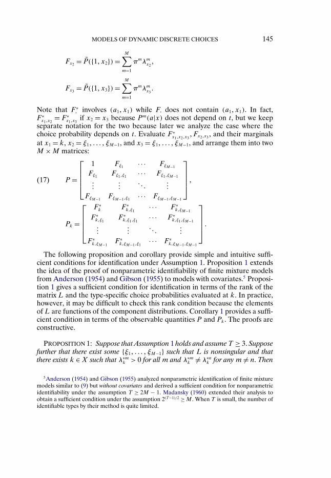
Fx2 = P({1�x2}) =M∑
m=1
πmλmx2�
Fx3 = P({1�x3}) =M∑
m=1
πmλmx3�
Note that F∗· involves (a1�x1) while F· does not contain (a1�x1). In fact,
F∗x1�x2
= F∗x1�x3
if x2 = x3 because Pm(a|x) does not depend on t, but we keepseparate notation for the two because later we analyze the case where thechoice probability depends on t. Evaluate F∗
x1�x2�x3�Fx2�x3 , and their marginals
at x1 = k, x2 = ξ1� � � � � ξM−1, and x3 = ξ1� � � � � ξM−1, and arrange them into twoM ×M matrices:
P =
⎡⎢⎢⎢⎣
1 Fξ1 · · · FξM−1
Fξ1 Fξ1�ξ1 · · · Fξ1�ξM−1
������
� � ����
FξM−1 FξM−1�ξ1 · · · FξM−1�ξM−1
⎤⎥⎥⎥⎦ �(17)
Pk =
⎡⎢⎢⎢⎣
F∗k F∗
k�ξ1· · · F∗
k�ξM−1
F∗k�ξ1
F∗k�ξ1�ξ1
· · · F∗k�ξ1�ξM−1
������
� � ����
F∗k�ξM−1
F∗k�ξM−1�ξ1
· · · F∗k�ξM−1�ξM−1
⎤⎥⎥⎥⎦ �
The following proposition and corollary provide simple and intuitive suffi-cient conditions for identification under Assumption 1. Proposition 1 extendsthe idea of the proof of nonparametric identifiability of finite mixture modelsfrom Anderson (1954) and Gibson (1955) to models with covariates.5 Proposi-tion 1 gives a sufficient condition for identification in terms of the rank of thematrix L and the type-specific choice probabilities evaluated at k. In practice,however, it may be difficult to check this rank condition because the elementsof L are functions of the component distributions. Corollary 1 provides a suffi-cient condition in terms of the observable quantities P and Pk. The proofs areconstructive.
PROPOSITION 1: Suppose that Assumption 1 holds and assume T ≥ 3. Supposefurther that there exist some {ξ1� � � � � ξM−1} such that L is nonsingular and thatthere exists k ∈X such that λ∗m
k > 0 for all m and λ∗mk = λ∗n
k for any m = n. Then
5Anderson (1954) and Gibson (1955) analyzed nonparametric identification of finite mixturemodels similar to (9) but without covariates and derived a sufficient condition for nonparametricidentifiability under the assumption T ≥ 2M − 1. Madansky (1960) extended their analysis toobtain a sufficient condition under the assumption 2(T−1)/2 ≥ M . When T is small, the number ofidentifiable types by their method is quite limited.
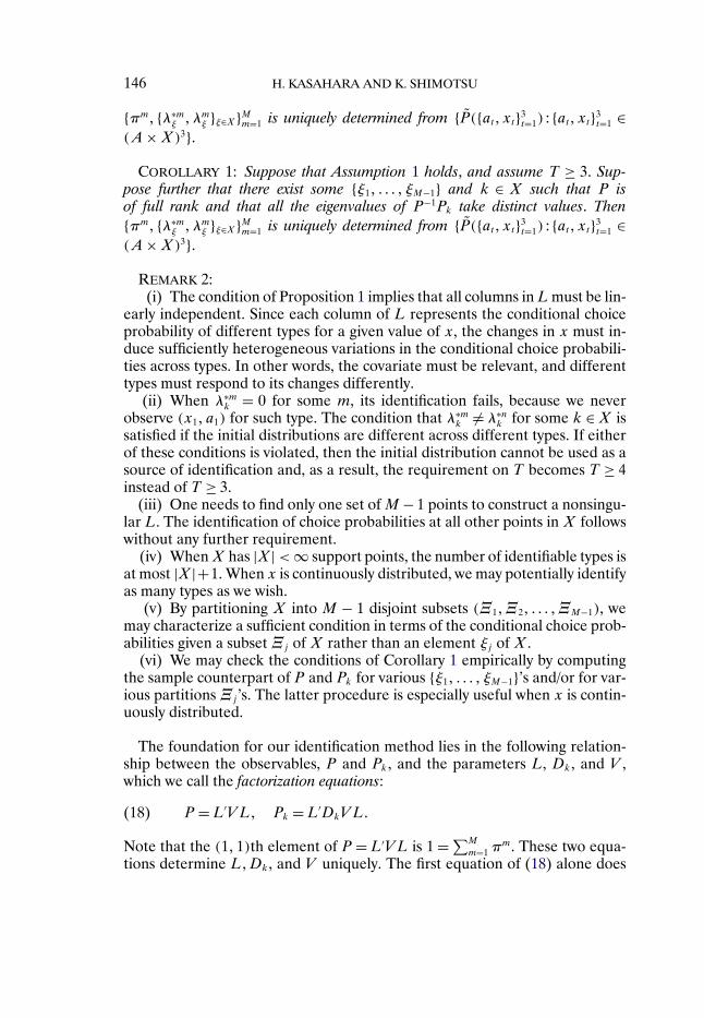
146 H. KASAHARA AND K. SHIMOTSU
{πm� {λ∗mξ �λm
ξ }ξ∈X}Mm=1 is uniquely determined from {P({at�xt}3t=1) : {at�xt}3
t=1 ∈(A×X)3}.
COROLLARY 1: Suppose that Assumption 1 holds, and assume T ≥ 3. Sup-pose further that there exist some {ξ1� � � � � ξM−1} and k ∈ X such that P isof full rank and that all the eigenvalues of P−1Pk take distinct values. Then{πm� {λ∗m
ξ �λmξ }ξ∈X}Mm=1 is uniquely determined from {P({at�xt}3
t=1) : {at�xt}3t=1 ∈
(A×X)3}.REMARK 2:
(i) The condition of Proposition 1 implies that all columns in L must be lin-early independent. Since each column of L represents the conditional choiceprobability of different types for a given value of x, the changes in x must in-duce sufficiently heterogeneous variations in the conditional choice probabili-ties across types. In other words, the covariate must be relevant, and differenttypes must respond to its changes differently.
(ii) When λ∗mk = 0 for some m, its identification fails, because we never
observe (x1� a1) for such type. The condition that λ∗mk = λ∗n
k for some k ∈ X issatisfied if the initial distributions are different across different types. If eitherof these conditions is violated, then the initial distribution cannot be used as asource of identification and, as a result, the requirement on T becomes T ≥ 4instead of T ≥ 3.
(iii) One needs to find only one set of M − 1 points to construct a nonsingu-lar L. The identification of choice probabilities at all other points in X followswithout any further requirement.
(iv) When X has |X|<∞ support points, the number of identifiable types isat most |X|+1. When x is continuously distributed, we may potentially identifyas many types as we wish.
(v) By partitioning X into M − 1 disjoint subsets (Ξ1�Ξ2� � � � �ΞM−1), wemay characterize a sufficient condition in terms of the conditional choice prob-abilities given a subset Ξj of X rather than an element ξj of X .
(vi) We may check the conditions of Corollary 1 empirically by computingthe sample counterpart of P and Pk for various {ξ1� � � � � ξM−1}’s and/or for var-ious partitions Ξj ’s. The latter procedure is especially useful when x is contin-uously distributed.
The foundation for our identification method lies in the following relation-ship between the observables, P and Pk, and the parameters L, Dk, and V ,which we call the factorization equations:
P =L′V L� Pk = L′DkV L�(18)
Note that the (1�1)th element of P = L′V L is 1 = ∑M
m=1 πm. These two equa-
tions determine L�Dk, and V uniquely. The first equation of (18) alone does
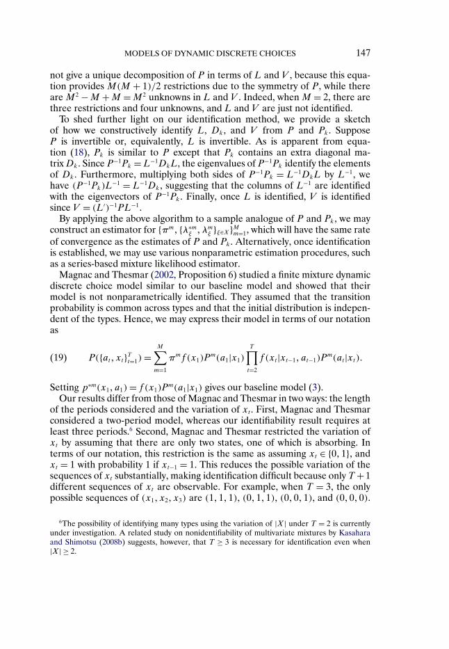
MODELS OF DYNAMIC DISCRETE CHOICES 147
not give a unique decomposition of P in terms of L and V , because this equa-tion provides M(M + 1)/2 restrictions due to the symmetry of P , while thereare M2 −M +M = M2 unknowns in L and V . Indeed, when M = 2, there arethree restrictions and four unknowns, and L and V are just not identified.
To shed further light on our identification method, we provide a sketchof how we constructively identify L, Dk, and V from P and Pk. SupposeP is invertible or, equivalently, L is invertible. As is apparent from equa-tion (18), Pk is similar to P except that Pk contains an extra diagonal ma-trix Dk. Since P−1Pk =L−1DkL, the eigenvalues of P−1Pk identify the elementsof Dk. Furthermore, multiplying both sides of P−1Pk = L−1DkL by L−1, wehave (P−1Pk)L
−1 = L−1Dk, suggesting that the columns of L−1 are identifiedwith the eigenvectors of P−1Pk. Finally, once L is identified, V is identifiedsince V = (L′)−1PL−1.
By applying the above algorithm to a sample analogue of P and Pk, we mayconstruct an estimator for {πm� {λ∗m
ξ �λmξ }ξ∈X}Mm=1, which will have the same rate
of convergence as the estimates of P and Pk. Alternatively, once identificationis established, we may use various nonparametric estimation procedures, suchas a series-based mixture likelihood estimator.
Magnac and Thesmar (2002, Proposition 6) studied a finite mixture dynamicdiscrete choice model similar to our baseline model and showed that theirmodel is not nonparametrically identified. They assumed that the transitionprobability is common across types and that the initial distribution is indepen-dent of the types. Hence, we may express their model in terms of our notationas
P({at�xt}Tt=1)=M∑
m=1
πmf(x1)Pm(a1|x1)
T∏t=2
f (xt |xt−1� at−1)Pm(at |xt)�(19)
Setting p∗m(x1� a1)= f (x1)Pm(a1|x1) gives our baseline model (3).
Our results differ from those of Magnac and Thesmar in two ways: the lengthof the periods considered and the variation of xt . First, Magnac and Thesmarconsidered a two-period model, whereas our identifiability result requires atleast three periods.6 Second, Magnac and Thesmar restricted the variation ofxt by assuming that there are only two states, one of which is absorbing. Interms of our notation, this restriction is the same as assuming xt ∈ {0�1}, andxt = 1 with probability 1 if xt−1 = 1. This reduces the possible variation of thesequences of xt substantially, making identification difficult because only T +1different sequences of xt are observable. For example, when T = 3, the onlypossible sequences of (x1�x2�x3) are (1�1�1), (0�1�1), (0�0�1), and (0�0�0).
6The possibility of identifying many types using the variation of |X| under T = 2 is currentlyunder investigation. A related study on nonidentifiability of multivariate mixtures by Kasaharaand Shimotsu (2008b) suggests, however, that T ≥ 3 is necessary for identification even when|X| ≥ 2.
148 H. KASAHARA AND K. SHIMOTSU
If we assume T ≥ 3 and that there are more than two nonabsorbing states, thenwe can apply Proposition 1 and Corollary 1 to (19). Alternately, identifying thesingle nonabsorbing state model is still possible if T ≥ 2M − 1 by applying Re-mark 3 below with x= 0, although Remark 3 uses the stationarity of Pm(a|x).
For the sake of brevity, in the subsequent analysis we provide sufficient con-ditions only in terms of the rank of the matrix of the type-specific componentdistributions (e.g., L). In each of the following propositions, sufficient condi-tions in terms of the distribution function of the observed data can easily bededuced from the conditions in terms of the type-specific component distribu-tions.
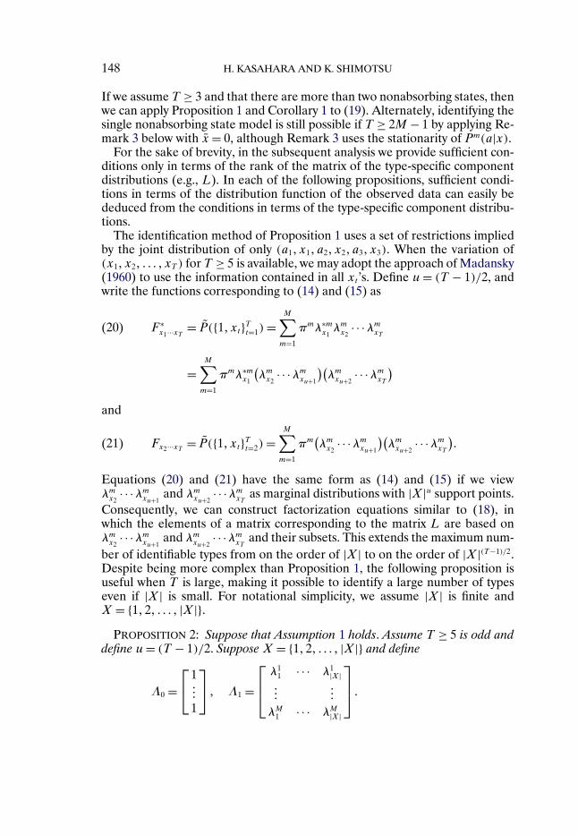
The identification method of Proposition 1 uses a set of restrictions impliedby the joint distribution of only (a1�x1� a2�x2� a3�x3). When the variation of(x1�x2� � � � � xT ) for T ≥ 5 is available, we may adopt the approach of Madansky(1960) to use the information contained in all xt ’s. Define u = (T − 1)/2, andwrite the functions corresponding to (14) and (15) as
F∗x1···xT = P({1�xt}Tt=1)=
M∑m=1
πmλ∗mx1λmx2
· · ·λmxT
(20)
=M∑
m=1
πmλ∗mx1
(λmx2
· · ·λmxu+1
)(λmxu+2
· · ·λmxT
)and
Fx2···xT = P({1�xt}Tt=2)=M∑
m=1
πm(λmx2
· · ·λmxu+1
)(λmxu+2
· · ·λmxT
)�(21)
Equations (20) and (21) have the same form as (14) and (15) if we viewλmx2
· · ·λmxu+1
and λmxu+2
· · ·λmxT
as marginal distributions with |X|u support points.Consequently, we can construct factorization equations similar to (18), inwhich the elements of a matrix corresponding to the matrix L are based onλmx2
· · ·λmxu+1
and λmxu+2
· · ·λmxT
and their subsets. This extends the maximum num-ber of identifiable types from on the order of |X| to on the order of |X|(T−1)/2.Despite being more complex than Proposition 1, the following proposition isuseful when T is large, making it possible to identify a large number of typeseven if |X| is small. For notational simplicity, we assume |X| is finite andX = {1�2� � � � � |X|}.
PROPOSITION 2: Suppose that Assumption 1 holds. Assume T ≥ 5 is odd anddefine u= (T − 1)/2. Suppose X = {1�2� � � � � |X|} and define
Λ0 =⎡⎣1���1
⎤⎦ � Λ1 =
⎡⎢⎣
λ11 · · · λ1
|X|���
���
λM1 · · · λM
|X|
⎤⎥⎦ �
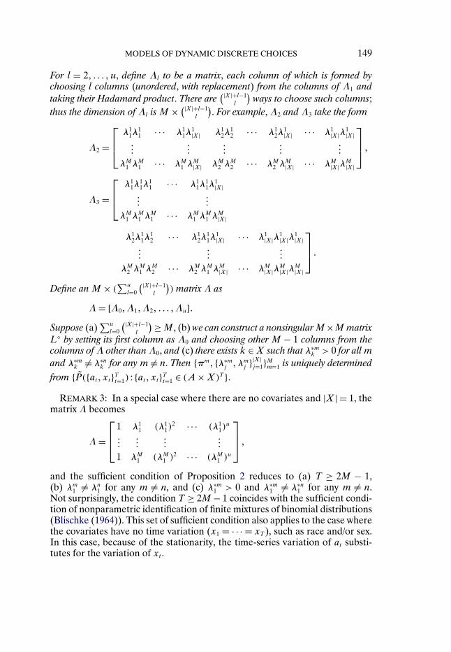
MODELS OF DYNAMIC DISCRETE CHOICES 149
For l = 2� � � � � u, define Λl to be a matrix, each column of which is formed bychoosing l columns (unordered, with replacement) from the columns of Λ1 andtaking their Hadamard product. There are
(|X|+l−1l
)ways to choose such columns;
thus the dimension of Λl is M × (|X|+l−1l
). For example, Λ2 and Λ3 take the form
Λ2 =⎡⎢⎣
λ11λ
11 · · · λ1
1λ1|X| λ1
2λ12 · · · λ1
2λ1|X| · · · λ1
|X|λ1|X|
������
������
���
λM1 λM
1 · · · λM1 λM
|X| λM2 λM
2 · · · λM2 λM
|X| · · · λM|X|λ
M|X|
⎤⎥⎦ �
Λ3 =⎡⎢⎣
λ11λ
11λ
11 · · · λ1
1λ11λ
1|X|
������
λM1 λM
1 λM1 · · · λM
1 λM1 λM
|X|
λ12λ
11λ
12 · · · λ1
2λ11λ
1|X| · · · λ1
|X|λ1|X|λ
1|X|
������
���
λM2 λM
1 λM2 · · · λM
2 λM1 λM
|X| · · · λM|X|λ
M|X|λ
M|X|
⎤⎥⎦ �
Define an M × (∑u
l=0
(|X|+l−1l
)) matrix Λ as
Λ= [Λ0�Λ1�Λ2� � � � �Λu]�Suppose (a)
∑u
l=0
(|X|+l−1l
) ≥M , (b) we can construct a nonsingular M×M matrixL by setting its first column as Λ0 and choosing other M − 1 columns from thecolumns of Λ other than Λ0, and (c) there exists k ∈ X such that λ∗m
k > 0 for all mand λ∗m
k = λ∗nk for any m = n. Then {πm� {λ∗m
j �λmj }|X|
j=1}Mm=1 is uniquely determinedfrom {P({at�xt}Tt=1) : {at�xt}Tt=1 ∈ (A×X)T }.
REMARK 3: In a special case where there are no covariates and |X| = 1, thematrix Λ becomes
Λ=⎡⎢⎣
1 λ11 (λ1
1)2 · · · (λ1
1)u
������
������
1 λM1 (λM
1 )2 · · · (λM1 )u
⎤⎥⎦ �
and the sufficient condition of Proposition 2 reduces to (a) T ≥ 2M − 1,(b) λm
1 = λn1 for any m = n, and (c) λ∗m
1 > 0 and λ∗m1 = λ∗n
1 for any m = n.Not surprisingly, the condition T ≥ 2M − 1 coincides with the sufficient condi-tion of nonparametric identification of finite mixtures of binomial distributions(Blischke (1964)). This set of sufficient condition also applies to the case wherethe covariates have no time variation (x1 = · · · = xT ), such as race and/or sex.In this case, because of the stationarity, the time-series variation of at substi-tutes for the variation of xt .
150 H. KASAHARA AND K. SHIMOTSU
Houde and Imai (2006) studied nonparametric identification of finite mix-ture dynamic discrete choice models by fixing the value of the covariate x (to x,for instance) and derived a sufficient condition for T . They also considered amodel with terminating state.
If the conditional choice probabilities of different types are heterogeneousand the column vectors (λ1
x� � � � � λMx )
′ for x = 1� � � � � |X| are linearly indepen-dent, the rank condition of this proposition is likely to be satisfied, since theHadamard products of these column vectors are unlikely to be linearly depen-dent, unless by chance.
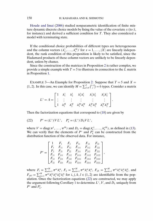
Since the construction of the matrices in Proposition 2 is rather complex, weprovide a simple example with T = 5 to illustrate its connection to the L matrixin Proposition 1.
EXAMPLE 3—An Example for Proposition 2: Suppose that T = 5 and X ={1�2}. In this case, we can identify M = ∑2
l=0
(1+l
l
) = 6 types. Consider a matrix
L =Λ =⎡⎢⎣
1 λ11 λ1
2 λ11λ
11 λ1
1λ12 λ1
2λ12
������
������
������
1 λM1 λM
2 λM1 λM
1 λM1 λM
2 λM2 λM
2
⎤⎥⎦ �
Then the factorization equations that correspond to (18) are given by
P = (L)′V L� Pk = (L)′DkV L�(22)
where V = diag(π1� � � � �πM) and Dk = diag(λ∗1k � � � � � λ
∗Mk ), as defined in (13).
We can verify that the elements of P and Pk can be constructed from the
distribution function of the observed data. For instance,
P =
⎡⎢⎢⎢⎢⎢⎣
1 F1 F2 F11 F12 F22
F1 F11 F12 F111 F112 F122
F2 F21 F22 F211 F212 F222
F11 F111 F112 F1111 F1112 F1122
F12 F121 F122 F1211 F1212 F1222
F22 F221 F222 F2211 F2212 F2222
⎤⎥⎥⎥⎥⎥⎦ �
where Fi = ∑M
m=1 πmλm
i , Fij = ∑M
m=1 πmλm
i λmj , Fijk = ∑M
m=1 πmλm
i λmj λ
mk , and
Fijkl = ∑M
m=1 πmλm
i λmj λ
mk λ
ml for i� j�k� l ∈ {1�2} are identifiable from the pop-
ulation. Once the factorization equations (22) are constructed, we may applythe argument following Corollary 1 to determine L, V , and Dk uniquely fromP and P
k .
MODELS OF DYNAMIC DISCRETE CHOICES 151
2.2. Identification of the Number of Types
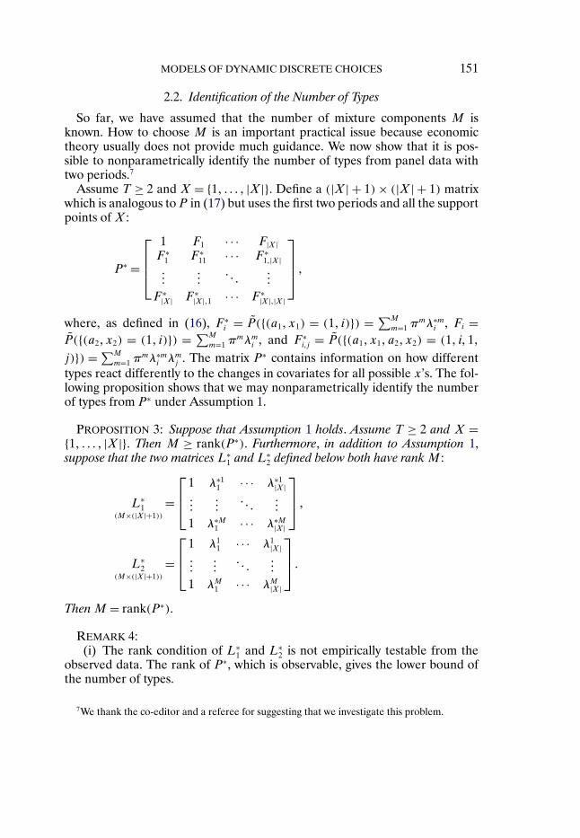
So far, we have assumed that the number of mixture components M isknown. How to choose M is an important practical issue because economictheory usually does not provide much guidance. We now show that it is pos-sible to nonparametrically identify the number of types from panel data withtwo periods.7
Assume T ≥ 2 and X = {1� � � � � |X|}. Define a (|X| + 1) × (|X| + 1) matrixwhich is analogous to P in (17) but uses the first two periods and all the supportpoints of X:
P∗ =
⎡⎢⎢⎣
1 F1 · · · F|X|F∗
1 F∗11 · · · F∗
1�|X|���
���� � �
���
F∗|X| F∗
|X|�1 · · · F∗|X|�|X|
⎤⎥⎥⎦ �
where, as defined in (16), F∗i = P({(a1�x1) = (1� i)}) = ∑M
m=1 πmλ∗m
i , Fi =P({(a2�x2) = (1� i)}) = ∑M
m=1 πmλm
i , and F∗i�j = P({(a1�x1� a2�x2) = (1� i�1�
j)}) = ∑M
m=1 πmλ∗m
i λmj . The matrix P∗ contains information on how different
types react differently to the changes in covariates for all possible x’s. The fol-lowing proposition shows that we may nonparametrically identify the numberof types from P∗ under Assumption 1.
PROPOSITION 3: Suppose that Assumption 1 holds. Assume T ≥ 2 and X ={1� � � � � |X|}. Then M ≥ rank(P∗). Furthermore, in addition to Assumption 1,suppose that the two matrices L∗
1 and L∗2 defined below both have rank M :
L∗1
(M×(|X|+1))=
⎡⎢⎣
1 λ∗11 · · · λ∗1
|X|���
���� � �
���
1 λ∗M1 · · · λ∗M
|X|
⎤⎥⎦ �
L∗2
(M×(|X|+1))=
⎡⎢⎣
1 λ11 · · · λ1
|X|���
���� � �
���
1 λM1 · · · λM
|X|
⎤⎥⎦ �
Then M = rank(P∗).
REMARK 4:(i) The rank condition of L∗
1 and L∗2 is not empirically testable from the
observed data. The rank of P∗, which is observable, gives the lower bound ofthe number of types.
7We thank the co-editor and a referee for suggesting that we investigate this problem.
152 H. KASAHARA AND K. SHIMOTSU
(ii) Surprisingly, two periods of panel data, rather than three periods, maysuffice for identifying the number of types.
(iii) The rank condition on L∗1 implies that no row of L∗
1 can be expressedas a linear combination of the other rows of L∗
1. The same applies to the rankcondition on L∗
2. Since the mth row of L∗1 or L∗
2 completely summarizes typem’s conditional choice probability within each period, this condition requiresthat the changes in x provide sufficient variation in the choice probabilitiesacross types and that no type is “redundant” in one-dimensional submodels.
(iv) The rank condition on L∗2 is equivalent to the rank condition on L in
Proposition 1 when X = {1� � � � � |X|}. In other words, rank(L∗2)=M if and only
if rank(L) =M .(v) We may partition X into disjoint subsets and compute P∗ with respect
to subsets of X rather than elements of X .(vi) When T ≥ 4, we may use an approach similar to Proposition 2 to con-
struct a (∑u
l=0
(|X|+l−1l
) × ∑u
l=0
(|X|+l−1l
)) matrix P∗ (similar to P in Example 3
but using (x1�x2) and (x3�x4)) and increase the number of identifiable M tothe order of |X|(T−1)/2.
3. EXTENSIONS OF THE BASELINE MODEL
In this section, we relax Assumption 1 of the baseline model in various waysto accommodate real-world applications. In the following subsections, we re-lax Assumption 1(a) and (e) (stationarity), Assumption 1(b) and (d) (type-invariant transition), and Assumption 1(c) (unrestricted transition) in turn andanalyze nonparametric identifiability of resulting models. In all cases, identifi-cation is achieved by constructing a version of the factorization equation sim-ilar to (18), specific to the model under consideration, and then applying anargument that follows the one presented in (18). The differences arise solelyfrom the ways in which the factorization equations are constructed across thevarious models.
3.1. Time-Dependent Conditional Choice Probabilities
The baseline model (8) assumes that conditional choice probabilities and thetransition function do not change over periods. However, the agent’s decisionrules may change over periods in some models, such as a model with time-specific aggregate shocks or a model of finitely lived individuals. In this sub-section, we keep the assumption of the common transition function, but relaxAssumption 1(a) and (e) to extend our analysis to models with time-dependentchoice probabilities.
When Assumption 1(a) and (e) (stationarity) are relaxed but Assump-tion 1(b) and (d) (conditional independence and type-invariant transition) aremaintained, the choice probabilities and the transition function are written as
MODELS OF DYNAMIC DISCRETE CHOICES 153
Pmt (at |xt�xt−1� at−1) = Pm
t (at |xt) and fmt (xt |{xτ�aτ}t−1
τ=1) = ft(xt |{xτ�aτ}t−1τ=1), re-
spectively, where at−1 is not an element of xt . Equation (9) then becomes
P({at�xt}Tt=1) = P({at�xt}Tt=1)T∏t=2
ft(xt |{xτ�aτ}t−1τ=1)
(23)
=M∑
m=1
πmp∗m(x1� a1)
T∏t=2
Pmt (at |xt)�
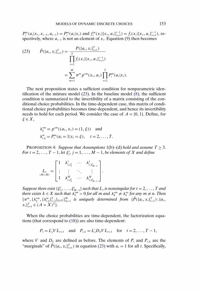
The next proposition states a sufficient condition for nonparametric iden-tification of the mixture model (23). In the baseline model (8), the sufficientcondition is summarized to the invertibility of a matrix consisting of the con-ditional choice probabilities. In the time-dependent case, this matrix of condi-tional choice probabilities becomes time-dependent, and hence its invertibilityneeds to hold for each period. We consider the case of A = {0�1}. Define, forξ ∈ X ,
λ∗mξ = p∗m((a1�x1)= (1� ξ)) and
λmt�ξ = Pm
t (at = 1|xt = ξ)� t = 2� � � � �T�
PROPOSITION 4: Suppose that Assumptions 1(b)–(d) hold and assume T ≥ 3.For t = 2� � � � � T − 1, let ξt
j , j = 1� � � � �M − 1, be elements of X and define
Lt(M×M)
=
⎡⎢⎢⎣
1 λ1t�ξt1
· · · λ1t�ξtM−1
������
� � ����
1 λMt�ξt1
· · · λMt�ξtM−1
⎤⎥⎥⎦ �
Suppose there exist {ξt1� � � � � ξ
tM−1} such that Lt is nonsingular for t = 2� � � � �T and
there exists k ∈X such that λ∗mk > 0 for all m and λ∗m
k = λ∗nk for any m = n. Then
{πm� {λ∗mξ � {λm
t�ξ}Tt=2}ξ∈X}Mm=1 is uniquely determined from {P({at�xt}Tt=1) : {at�
xt}Tt=1 ∈ (A×X)T }.
When the choice probabilities are time-dependent, the factorization equa-tions (that correspond to (18)) are also time-dependent:
Pt =L′tV Lt+1 and Pt�k =L′
tDkV Lt+1 for t = 2� � � � � T − 1�
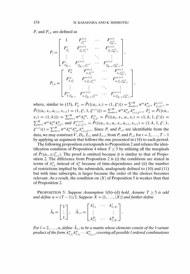
where V and Dk are defined as before. The elements of Pt and Pt�k are the“marginals” of P({at�xt}Tt=1) in equation (23) with at = 1 for all t. Specifically,
154 H. KASAHARA AND K. SHIMOTSU
Pt and Pt�k are defined as
Pt =
⎡⎢⎢⎢⎢⎢⎣
1 Ft+1ξt+1
1· · · Ft+1
ξt+1M−1
Ftξt1
Ft�t+1ξt1�ξ
t+11
· · · Ft�t+1ξt1�ξ
t+1M−1
������
� � ����
FtξtM−1
Ft�t+1ξtM−1�ξ
t+11
· · · Ft�t+1ξtM−1�ξ
t+1M−1
⎤⎥⎥⎥⎥⎥⎦ �
Pt�k =
⎡⎢⎢⎢⎢⎢⎣
F∗k F∗t+1
k�ξt+11
· · · F∗t+1k�ξt+1
M−1
F∗tk�ξt1
F∗t�t+1k�ξt1�ξ
t+11
· · · F∗t�t+1k�ξt1�ξ
t+1M−1
������
� � ����
F∗tk�ξtM−1
F∗t�t+1k�ξtM−1�ξ
t+11
· · · F∗t�t+1k�ξtM−1�ξ
t+1M−1
⎤⎥⎥⎥⎥⎥⎦ �
where, similar to (15), Ftξt = P({(at� xt) = (1� ξt)}) = ∑M
m=1 πmλm
t�ξt , Ft�t+1ξt �ξt+1 =
P({(at� xt� at+1�xt+1) = (1� ξt�1� ξt+1)}) = ∑M
m=1 πmλm
t�ξt λmt+1�ξt+1 , F∗
k = P({(a1�
x1) = (1�k)}) = ∑M
m=1 πmλ∗m
k , F∗tk�ξt = P({(a1�x1� at� xt) = (1�k�1� ξt)}) =∑M
m=1 πmλ∗m
k λmt�ξt , and F∗t�t+1
k�ξt �ξt+1 = P({(a1�x1� at� xt� at+1�xt+1) = (1�k�1� ξt�1�
ξt+1)}) = ∑M
m=1 πmλ∗m
k λmt�ξt λ
mt+1�ξt+1 . Since Pt and Pt�k are identifiable from the
data, we may construct V , Dk, Lt , and Lt+1 from Pt and Pt�k for t = 2� � � � �T −1by applying an argument that follows the one presented in (18) to each period.
The following proposition corresponds to Proposition 2 and relaxes the iden-tification condition of Proposition 4 when T ≥ 5 by utilizing all the marginalsof P({at�xt}Tt=1). The proof is omitted because it is similar to that of Propo-sition 2. The difference from Proposition 2 is (i) the conditions are stated interms of λm
t�ξ instead of λmξ because of time-dependence and (ii) the number
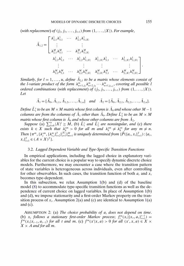
of restrictions implied by the submodels, analogously defined to (10) and (11)but with time subscripts, is larger because the order of the choices becomesrelevant. As a result, the condition on |X| of Proposition 5 is weaker than thatof Proposition 2.
PROPOSITION 5: Suppose Assumption 1(b)–(d) hold. Assume T ≥ 5 is oddand define u= (T − 1)/2. Suppose X = {1� � � � � |X|} and further define
Λ0 =⎡⎣1���1
⎤⎦ � Λ1�1 =
⎡⎢⎣λ1
2�1 · · · λ12�|X|
������
λM2�1 · · · λM
2�|X|
⎤⎥⎦ �
For l = 2� � � � � u, define Λ1�l to be a matrix whose elements consist of the l-variateproduct of the form λm
2�j2λm
3�j3· · ·λm
l�jl+1, covering all possible l ordered combinations
MODELS OF DYNAMIC DISCRETE CHOICES 155
(with replacement) of (j2� j3� � � � � jl+1) from (1� � � � � |X|). For example,
Λ1�2 =⎡⎢⎣λ1
2�1λ13�1 · · · λ1
2�1λ13�|X|
������
λM2�1λ
M3�1 · · · λM
2�1λM3�|X|
λ12�2λ
13�1 · · · λ1
2�2λ13�|X| λ1
2�|X|λ13�1 · · · λ1
2�|X|λ13�|X|
������
������
λM2�2λ
M3�1 · · · λM
2�2λM3�|X| λM
2�|X|λM3�1 · · · λM
2�|X|λM3�|X|
⎤⎥⎦ �
Similarly, for l = 1� � � � � u, define Λ2�l to be a matrix whose elements consist ofthe l-variate product of the form λm
u+1�j2λmu+2�j3
· · ·λmu+l�jl+1
, covering all possible l
ordered combinations (with replacement) of (j2� j3� � � � � jl+1) from (1� � � � � |X|).Let
Λ1 = [Λ0� Λ1�1� Λ1�2� � � � � Λ1�u] and Λ2 = [Λ0� Λ2�1� Λ2�2� � � � � Λ2�u]�Define L
1 to be an M×M matrix whose first column is Λ0 and whose other M−1columns are from the columns of Λ1 other than Λ0. Define L
2 to be an M × M
matrix whose first column is Λ0 and whose other columns are from Λ2.Suppose (a)
∑u
l=0 |X|l ≥ M , (b) L1 and L
2 are nonsingular, and (c) thereexists k ∈ X such that λ∗m
k > 0 for all m and λ∗mk = λ∗n
k for any m = n.Then {πm� {λ∗m
j � {λmt�j}Tt=2}|X|
j=1}Mm=1 is uniquely determined from {P({at�xt}Tt=1) : {at�
xt}Tt=1 ∈ (A×X)T }.
3.2. Lagged Dependent Variable and Type-Specific Transition Functions
In empirical applications, including the lagged choice in explanatory vari-ables for the current choice is a popular way to specify dynamic discrete choicemodels. Furthermore, we may encounter a case where the transition patternof state variables is heterogeneous across individuals, even after controllingfor other observables. In such cases, the transition function of both at and xt
becomes type-dependent.In this subsection, we relax Assumption 1(b) and (d) of the baseline
model (8) to accommodate type-specific transition functions as well as the de-pendence of current choice on lagged variables. In place of Assumption 1(b)and (d), we impose stationarity and a first-order Markov property on the tran-sition process of xt . Assumption 2(a) and (c) are identical to Assumption 1(a)and (c).
ASSUMPTION 2: (a) The choice probability of at does not depend on time.(b) xt follows a stationary first-order Markov process; fm
t (xt |{xτ�aτ}t−1τ=1) =
fm(xt |xt−1� at−1) for all t and m. (c) fm(x′|x�a) > 0 for all (x′�x�a) ∈ X ×X ×A and for all m.
156 H. KASAHARA AND K. SHIMOTSU
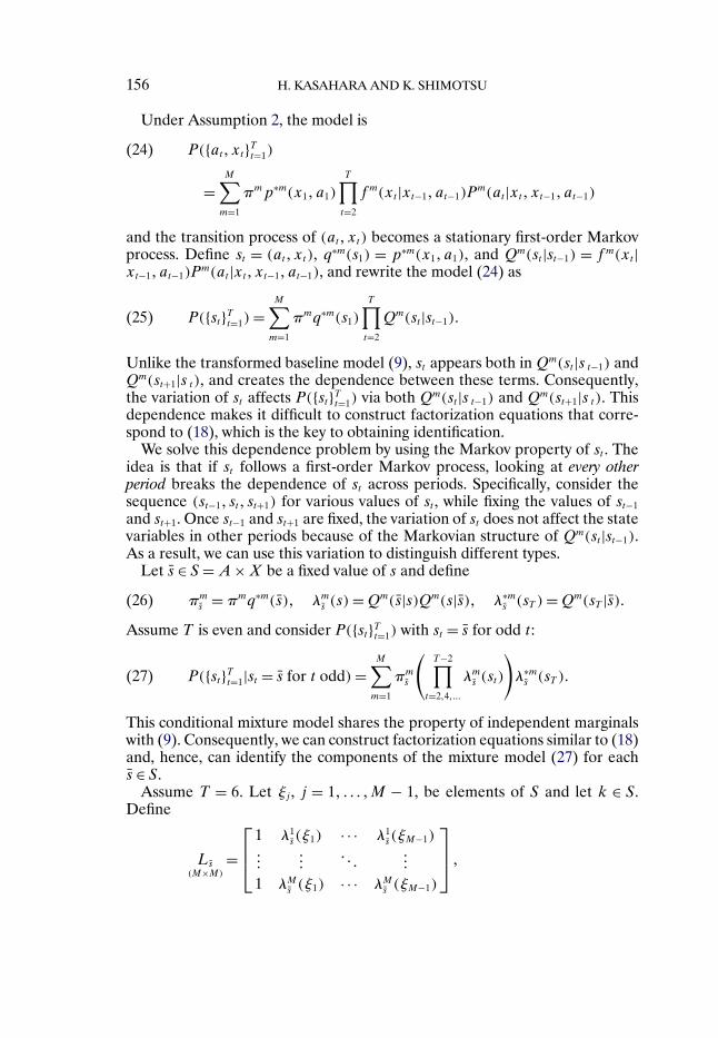
Under Assumption 2, the model is
P({at�xt}Tt=1)(24)
=M∑
m=1
πmp∗m(x1� a1)
T∏t=2
fm(xt |xt−1� at−1)Pm(at |xt�xt−1� at−1)
and the transition process of (at� xt) becomes a stationary first-order Markovprocess. Define st = (at� xt), q∗m(s1) = p∗m(x1� a1), and Qm(st |st−1) = fm(xt |xt−1� at−1)P
m(at |xt�xt−1� at−1), and rewrite the model (24) as
P({st}Tt=1)=M∑
m=1
πmq∗m(s1)
T∏t=2
Qm(st |st−1)�(25)
Unlike the transformed baseline model (9), st appears both in Qm(st |s t−1) andQm(st+1|s t), and creates the dependence between these terms. Consequently,the variation of st affects P({st}Tt=1) via both Qm(st |s t−1) and Qm(st+1|s t). Thisdependence makes it difficult to construct factorization equations that corre-spond to (18), which is the key to obtaining identification.
We solve this dependence problem by using the Markov property of st . Theidea is that if st follows a first-order Markov process, looking at every otherperiod breaks the dependence of st across periods. Specifically, consider thesequence (st−1� st� st+1) for various values of st , while fixing the values of st−1
and st+1. Once st−1 and st+1 are fixed, the variation of st does not affect the statevariables in other periods because of the Markovian structure of Qm(st |st−1).As a result, we can use this variation to distinguish different types.
Let s ∈ S = A×X be a fixed value of s and define
πms = πmq∗m(s)� λm
s (s) =Qm(s|s)Qm(s|s)� λ∗ms (sT )= Qm(sT |s)�(26)
Assume T is even and consider P({st}Tt=1) with st = s for odd t:
P({st}Tt=1|st = s for t odd)=M∑
m=1
πms
(T−2∏
t=2�4����
λms (st)
)λ∗ms (sT )�(27)
This conditional mixture model shares the property of independent marginalswith (9). Consequently, we can construct factorization equations similar to (18)and, hence, can identify the components of the mixture model (27) for eachs ∈ S.
Assume T = 6. Let ξj , j = 1� � � � �M − 1, be elements of S and let k ∈ S.Define
Ls(M×M)
=⎡⎢⎣
1 λ1s (ξ1) · · · λ1
s (ξM−1)���
���� � �
���
1 λMs (ξ1) · · · λM
s (ξM−1)
⎤⎥⎦ �
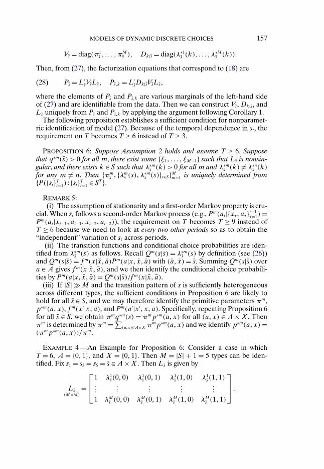
MODELS OF DYNAMIC DISCRETE CHOICES 157
Vs = diag(π1s � � � � �π
Ms )� Dk|s = diag(λ∗1
s (k)� � � � � λ∗Ms (k))�
Then, from (27), the factorization equations that correspond to (18) are
Ps = L′sVsLs� Ps�k =L′
sDk|sVsLs�(28)
where the elements of Ps and Ps�k are various marginals of the left-hand sideof (27) and are identifiable from the data. Then we can construct Vs, Dk|s, andLs uniquely from Ps and Ps�k by applying the argument following Corollary 1.
The following proposition establishes a sufficient condition for nonparamet-ric identification of model (27). Because of the temporal dependence in st , therequirement on T becomes T ≥ 6 instead of T ≥ 3.
PROPOSITION 6: Suppose Assumption 2 holds and assume T ≥ 6. Supposethat q∗m(s) > 0 for all m, there exist some {ξ1� � � � � ξM−1} such that Ls is nonsin-gular, and there exists k ∈ S such that λ∗m
s (k) > 0 for all m and λ∗ms (k) = λ∗n
s (k)for any m = n. Then {πm
s � {λms (s)�λ
∗ms (s)}s∈S}Mm=1 is uniquely determined from
{P({st}Tt=1) : {st}Tt=1 ∈ ST }.REMARK 5:
(i) The assumption of stationarity and a first-order Markov property is cru-cial. When st follows a second-order Markov process (e.g., Pm(at |{xτ�aτ}t−1
τ=1)=Pm(at |xt−1� at−1�xt−2� at−2)), the requirement on T becomes T ≥ 9 instead ofT ≥ 6 because we need to look at every two other periods so as to obtain the“independent” variation of st across periods.
(ii) The transition functions and conditional choice probabilities are iden-tified from λ∗m
s (s) as follows. Recall Qm(s|s) = λ∗ms (s) by definition (see (26))
and Qm(s|s) = fm(x|x� a)Pm(a|x� x� a) with (a� x) = s. Summing Qm(s|s) overa ∈ A gives fm(x|x� a), and we then identify the conditional choice probabili-ties by Pm(a|x� x� a)=Qm(s|s)/fm(x|x� a).
(iii) If |S| � M and the transition pattern of s is sufficiently heterogeneousacross different types, the sufficient conditions in Proposition 6 are likely tohold for all s ∈ S, and we may therefore identify the primitive parameters πm,p∗m(a�x), fm(x′|x�a), and Pm(a′|x′�x�a). Specifically, repeating Proposition 6for all s ∈ S, we obtain πmq∗m(s) = πmp∗m(a�x) for all (a�x) ∈ A × X . Thenπm is determined by πm = ∑
(a�x)∈A×X πmp∗m(a�x) and we identify p∗m(a�x) =(πmp∗m(a�x))/πm.
EXAMPLE 4 —An Example for Proposition 6: Consider a case in whichT = 6, A = {0�1}, and X = {0�1}. Then M = |S| + 1 = 5 types can be iden-tified. Fix s1 = s3 = s5 = s ∈A×X . Then Ls is given by
Ls(M×M)
=⎡⎢⎣
1 λ1s (0�0) λ1
s (0�1) λ1s (1�0) λ1
s (1�1)���
������
������
1 λMs (0�0) λM
s (0�1) λMs (1�0) λM
s (1�1)
⎤⎥⎦ �
158 H. KASAHARA AND K. SHIMOTSU
For example, the (5�5)th elements of Ps and Ps�k in (28) are given by P({s1 =s3 = s5 = s� s2 = s4 = (1�1)}) = ∑5
m=1 πms (λ
ms (1�1))2 and P({s1 = s3 = s5 =
s� s2 = s4 = (1�1)� s6 = k})= ∑5m=1 π
ms (λ
ms (1�1))2λ∗m
s (k), respectively.
When T ≥ 8, we can relax the condition |S| ≥ M − 1 of Proposition 6 byapplying the approach of Proposition 2. Define λ∗m
s (s) = Qm(s|s), λms�1(s1) =
Qm(s|s1)Qm(s1|s), and λm
s�2(s1� s2) = Qm(s|s1)Qm(s1|s2)Q
m(s2|s), and similarlydefine λm
s�l(s1� � � � � sl) for l ≥ 3 as an (l + 1)-variate product of Qm(s′|s)’s ofthe form Qm(s|s1) · · ·Qm(sl−1|sl)Qm(sl|s) for {st}lt=1 ∈ Sl.
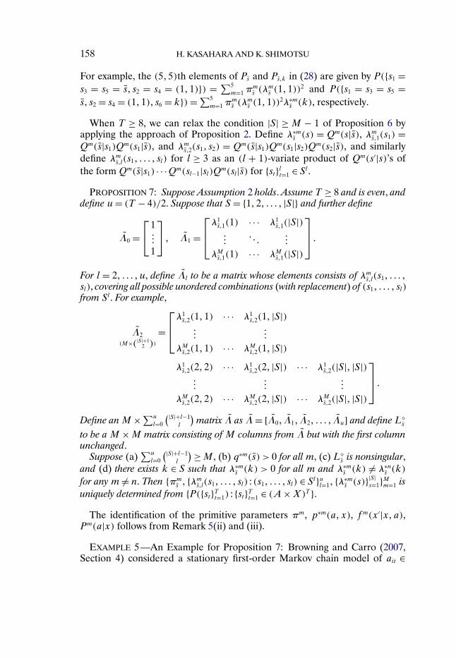
PROPOSITION 7: Suppose Assumption 2 holds. Assume T ≥ 8 and is even, anddefine u= (T − 4)/2. Suppose that S = {1�2� � � � � |S|} and further define
Λ0 =⎡⎣1���1
⎤⎦ � Λ1 =
⎡⎢⎣λ1s�1(1) · · · λ1
s�1(|S|)���
� � ����
λMs�1(1) · · · λM
s�1(|S|)
⎤⎥⎦ �
For l = 2� � � � � u, define Λl to be a matrix whose elements consists of λms�l(s1� � � � �
sl), covering all possible unordered combinations (with replacement) of (s1� � � � � sl)from Sl. For example,
Λ2(M×(|S|+1
2 ))=
⎡⎢⎣λ1s�2(1�1) · · · λ1
s�2(1� |S|)���
���
λMs�2(1�1) · · · λM
s�2(1� |S|)λ1s�2(2�2) · · · λ1
s�2(2� |S|) · · · λ1s�2(|S|� |S|)
������
���
λMs�2(2�2) · · · λM
s�2(2� |S|) · · · λMs�2(|S|� |S|)
⎤⎥⎦ �
Define an M × ∑u
l=0
(|S|+l−1l
)matrix Λ as Λ = [Λ0� Λ1� Λ2� � � � � Λu] and define L
s
to be a M ×M matrix consisting of M columns from Λ but with the first columnunchanged.
Suppose (a)∑u
l=0
(|S|+l−1l
) ≥M , (b) q∗m(s) > 0 for all m, (c) Ls is nonsingular,
and (d) there exists k ∈ S such that λ∗ms (k) > 0 for all m and λ∗m
s (k) = λ∗ns (k)
for any m = n. Then {πms � {λm
s�l(s1� � � � � sl) : (s1� � � � � sl) ∈ Sl}ul=1� {λ∗ms (s)}|S|
s=1}Mm=1 isuniquely determined from {P({st}Tt=1) : {st}Tt=1 ∈ (A×X)T }.
The identification of the primitive parameters πm, p∗m(a�x), fm(x′|x�a),Pm(a|x) follows from Remark 5(ii) and (iii).
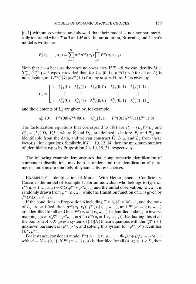
EXAMPLE 5—An Example for Proposition 7: Browning and Carro (2007,Section 4) considered a stationary first-order Markov chain model of ait ∈
MODELS OF DYNAMIC DISCRETE CHOICES 159
{0�1} without covariates and showed that their model is not nonparametri-cally identified when T = 3 and M = 9. In our notation, Browning and Carro’smodel is written as
P(a1� � � � � aT )=M∑
m=1
πmp∗m(a1)
T∏t=2
Pm(at |at−1)�
Note that s = a because there are no covariates. If T = 8, we can identify M =∑u
l=0
(2+l−1l
) = 6 types, provided that, for s = {0�1}, p∗m(s) > 0 for all m, Ls is
nonsingular, and Pm(1|s) = Pn(1|s) for any m = n. Here, Ls is given by
Ls =
⎡⎢⎣
1 λ1s�1(0) λ1
s�1(1) λ1s�2(0�0) λ1
s�2(0�1) λ1s�2(1�1)
������
������
������
1 λMs�1(0) λM
s�1(1) λMs�2(0�0) λM
s�2(0�1) λMs�2(1�1)
⎤⎥⎦
and the elements of L0 are given by, for example,
λm0�1(0)= Pm(0|0)Pm(0|0)� λm
0�2(1�1)= Pm(0|1)Pm(1|1)Pm(1|0)�The factorization equations that correspond to (18) are P
s = (Ls )
′VsLs and
Ps�k = (L
s )′Dk|sVsL
s , where Vs and Dk|s are defined as before. P
s and Ps�k are
identifiable from the data, and we can construct Vs, Dk|s, and Ls from these
factorization equations. Similarly, if T = 10�12�14, then the maximum numberof identifiable types by Proposition 7 is 10�15�21, respectively.
The following example demonstrates that nonparametric identification ofcomponent distributions may help us understand the identification of para-metric finite mixture models of dynamic discrete choices.
EXAMPLE 6 —Identification of Models With Heterogeneous Coefficients:Consider the model of Example 1. For an individual who belongs to type m,Pm(at = 1|xt� at−1) = Φ(x′
tβm + ρmat−1) and the initial observation, (a1�x1), is
randomly drawn from p∗m(a1�x1) while the transition function of xt is given byfm(xt |xt−1� at−1).
If the conditions in Proposition 6 including T ≥ 6, |S| ≥ M − 1, and the rankof Ls are satisfied, then p∗m(a1�x1), fm(xt |xt−1� at−1), and Pm(at = 1|xt� at−1)are identified for all m. Once Pm(at = 1|xt� at−1) is identified, taking an inversemapping gives x′
tβm + ρmat−1 =Φ−1(Pm(at = 1|xt� at−1)). Evaluating this at all
the points in A×X gives a system of |A||X| linear equations with dim(βm)+1unknown parameters (βm�ρm), and solving this system for (βm�ρm) identifies(βm�ρm).
For instance, consider a model Pm(at = 1|xt� at−1)=Φ(βm0 +βm
1 xt +ρmat−1)with A =X = {0�1}. If Pm(at = 1|x�a) is identified for all (a�x) ∈ A×X , then
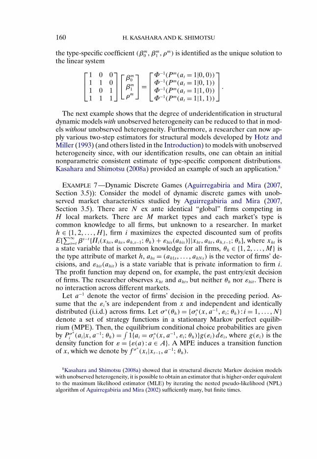
160 H. KASAHARA AND K. SHIMOTSU
the type-specific coefficient (βm0 �β
m1 �ρ
m) is identified as the unique solution tothe linear system⎡
⎢⎣1 0 01 1 01 0 11 1 1
⎤⎥⎦
⎡⎣βm
0
βm1
ρm
⎤⎦ =
⎡⎢⎣Φ−1(Pm(at = 1|0�0))Φ−1(Pm(at = 1|0�1))Φ−1(Pm(at = 1|1�0))Φ−1(Pm(at = 1|1�1))
⎤⎥⎦ �
The next example shows that the degree of underidentification in structuraldynamic models with unobserved heterogeneity can be reduced to that in mod-els without unobserved heterogeneity. Furthermore, a researcher can now ap-ply various two-step estimators for structural models developed by Hotz andMiller (1993) (and others listed in the Introduction) to models with unobservedheterogeneity since, with our identification results, one can obtain an initialnonparametric consistent estimate of type-specific component distributions.Kasahara and Shimotsu (2008a) provided an example of such an application.8
EXAMPLE 7 —Dynamic Discrete Games (Aguirregabiria and Mira (2007,Section 3.5)): Consider the model of dynamic discrete games with unob-served market characteristics studied by Aguirregabiria and Mira (2007,Section 3.5). There are N ex ante identical “global” firms competing inH local markets. There are M market types and each market’s type iscommon knowledge to all firms, but unknown to a researcher. In marketh ∈ {1�2� � � � �H}, firm i maximizes the expected discounted sum of profitsE[∑∞
s=t βs−t{Πi(xhs� ahs� ah�s−1;θh) + εhis(ahis)}|xht� aht� ah�t−1;θh], where xht is
a state variable that is common knowledge for all firms, θh ∈ {1�2� � � � �M} isthe type attribute of market h, ahs = (ah1s� � � � � ahNs) is the vector of firms’ de-cisions, and εhit(ahit) is a state variable that is private information to firm i.The profit function may depend on, for example, the past entry/exit decisionof firms. The researcher observes xht and aht , but neither θh nor εhit . There isno interaction across different markets.
Let a−1 denote the vector of firms’ decision in the preceding period. As-sume that the εi’s are independent from x and independent and identicallydistributed (i.i.d.) across firms. Let σ∗(θh) = {σ∗
i (x�a−1� εi;θh) : i = 1� � � � �N}
denote a set of strategy functions in a stationary Markov perfect equilib-rium (MPE). Then, the equilibrium conditional choice probabilities are givenby Pσ∗
i (ai|x�a−1;θh) = ∫1{ai = σ∗
i (x�a−1� εi;θh)}g(εi)dεi, where g(εi) is the
density function for ε = {ε(a) :a ∈ A}. A MPE induces a transition functionof x, which we denote by f σ∗
(xt |xt−1� a−1;θh).
8Kasahara and Shimotsu (2008a) showed that in structural discrete Markov decision modelswith unobserved heterogeneity, it is possible to obtain an estimator that is higher-order equivalentto the maximum likelihood estimator (MLE) by iterating the nested pseudo-likelihood (NPL)algorithm of Aguirregabiria and Mira (2002) sufficiently many, but finite times.
MODELS OF DYNAMIC DISCRETE CHOICES 161
Suppose that panel data {{aht� xht}Tt=1}Hh=1 are available. As in Aguirregabiriaand Mira (2007), consider the case where H → ∞ with N and T fixed. The ini-tial distribution of (a�x) differs across market types and is given by p∗m(a�x).Let Pm(aht |xht� ah�t−1) = ∏N
i=1 Pσ∗i (ahit |xht� ah�t−1;m) and fm(xht |xh�t−1�
ah�t−1) = f σ∗(xht |xh�t−1� ah�t−1;m). Then the likelihood function for market h
becomes a mixture across different unobserved market types,
P({aht� xht}Tt=1)
=M∑
m=1
πmp∗m(ah1�xh1)
T∏t=2
Pm(aht |xht� ah�t−1)fm(xht |xh�t−1� ah�t−1)�
for which Propositions 6 and 7 are applicable.
EXAMPLE 8—An Empirical Example of Aguirregabiria and Mira (2007, Sec-tion 5): Aguirregabiria and Mira (2007, Section 5) considered an empiricalmodel of entry and exit in local retail markets based on the model of Example7. Each market is indexed by h. The firms’ profits depend on the logarithmof the market size, xht , and their current and past entry/exit decisions, aht andah�t−1. The profit of a nonactive firm is zero. When active, firm i’s profit isΠo
i (xht� aht� ah�t−1) + ωh + εhit(ahit), where the function Πoi is common across
all the markets and εhit is i.i.d. across markets. The parameter ωh capturesthe unobserved market characteristics and has a discrete distribution with 21points of support. The logarithm of market size follows an exogenous first-order Markov process.
Their panel covers 6 years at annual frequency (i.e., T = 6). This satisfiesthe requirement for T in Proposition 6. Given the nonlinear nature of the dy-namic games models, the rank condition on the Ls matrix in Proposition 6 islikely to be satisfied. In their specification however, the transition function forxht , fh(xht |xh�t−1), is market-specific, so that the number of types is equal to thenumber of markets. Consequently, Proposition 6 does not apply to this case,and the type-specific conditional choice probabilities may not be nonparamet-rically identified.9
If we limit the number of types for transition functions, then we may ap-ply Proposition 6 to identify the type-specific conditional choice probabilitiesand the type-specific transition probabilities. For the mth type market, thejoint conditional choice probabilities across all firms are Pm(aht |xht� ah�t−1) =
9Aguirregabiria and Mira estimated the market-specific transition function using 14 years ofdata on market size from other data sources. Given the relatively long time length, the identifi-cation of market-specific transition functions may come from the time variation of each market.When the transition function is market-specific, however, the conditional choice probabilities alsobecome market-specific, leading to the incidental parameter problem. Even if the market-specifictransition function is known, nonparametrically identifying the market-specific conditional choiceprobabilities is not possible given a short panel.
162 H. KASAHARA AND K. SHIMOTSU
∏N
i=1 Pi(ahit |xht� ah�t−1;θm), where aht = (ah1t � � � � � ahNt)′. The market size is dis-
cretized with 10 support points (i.e., |X| = 10) and A = {0�1}N . Consequently,the size of the state space of sht = (aht� xht) for this model is |A||X| = 2N × 10,and we may identify up to M = 2N × 10 + 1 types. For instance, their Table VIreports that 63.5 percent of markets have no less than five potential firms (i.e.,N ≥ 5) in the restaurant industry. Hence, M = 25 × 10 + 1 = 321 market typescan be identified for these markets.10
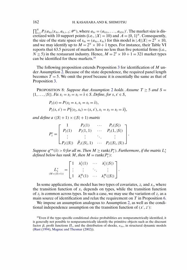
The following proposition extends Proposition 3 for identification of M un-der Assumption 2. Because of the state dependence, the required panel lengthbecomes T = 5. We omit the proof because it is essentially the same as that ofProposition 3.
PROPOSITION 8: Suppose that Assumption 2 holds. Assume T ≥ 5 and S ={1� � � � � |S|}. Fix s1 = s3 = s5 = s ∈ S. Define, for s� s′ ∈ S,
Ps(s) = P(s2 = s� s1 = s3 = s)�
Ps(s� s′)= P
((s2� s4)= (s� s′)� s1 = s3 = s5 = s
)�
and define a (|S| + 1)× (|S| + 1) matrix
P∗s =
⎡⎢⎢⎣
1 Ps(1) · · · Ps(|S|)Ps(1) Ps(1�1) · · · Ps(1� |S|)���
���� � �
���
Ps(|S|) Ps(|S|�1) · · · Ps(|S|� |S|)
⎤⎥⎥⎦ �
Suppose q∗m(s) > 0 for all m. Then M ≥ rank(P∗s ). Furthermore, if the matrix L∗
s
defined below has rank M , then M = rank(P∗s ):
L∗s
(M×(|S|+1))=
⎡⎢⎣
1 λ1s (1) · · · λ1
s (|S|)���
���� � �
���
1 λMs (1) · · · λM
s (|S|)
⎤⎥⎦ �
In some applications, the model has two types of covariates, zt and xt , wherethe transition function of xt depends on types, while the transition functionof zt is common across types. In such a case, we may use the variation of zt as amain source of identification and relax the requirement on T in Proposition 6.
We impose an assumption analogous to Assumption 2, as well as the condi-tional independence assumption on the transition function of (x′� z′):
10Even if the type-specific conditional choice probabilities are nonparametrically identified, itis generally not possible to nonparametrically identify the primitive objects such as the discountfactor β, profit functions Πi , and the distribution of shocks, εiht , in structural dynamic models(Rust (1994), Magnac and Thesmar (2002)).
MODELS OF DYNAMIC DISCRETE CHOICES 163
ASSUMPTION 3: (a) The choice probability of at does not depend on timeand is independent of zt−1. (b) The transition function of (xt� zt) conditionalon {xτ� zτ� aτ}t−1
τ=1 takes the form g(zt |xt−1� zt−1� at−1)fm(xt |xt−1� at−1) for all t.
(c) fm(x′|x�a) > 0 for all (x′�x�a) ∈ X × X × A and g(z′|x�z�a) > 0 for all(z′�x� z�a) ∈Z ×X ×Z ×A and for m = 1� � � � �M .
Under Assumption 3, consider a model
P({at�xt� zt}Tt=1)
=M∑
m=1
πmp∗m(x1� z1� a1)
T∏t=2
g(zt |xt−1� zt−1� at−1)fm(xt |xt−1� at−1)
× Pm(at |xt�xt−1� at−1� zt)�
Assuming g(zt |xt−1� zt−1� at−1) is known and defining st = (at� xt), q∗m(s1�
z1) = p∗m(x1� z1� a1), and Qm(st |st−1� zt) = fm(xt |xt−1� at−1)Pm(at |xt�xt−1� at−1�
zt), we can write this equation as
P({st� zt}Tt=1) = P({at�xt� zt}Tt=1)T∏t=2
g(zt |xt−1� zt−1� at−1)
(29)
=M∑
m=1
πmq∗m(s1� z1)
T∏t=2
Qm(st |st−1� zt)�
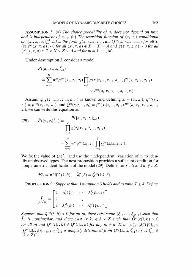
We fix the value of {st}Tt=1 and use the “independent” variation of zt to iden-tify unobserved types. The next proposition provides a sufficient condition fornonparametric identification of the model (29). Define, for s ∈ S and h�ξ ∈ Z,
πms�h = πmq∗m(s�h)� λm
s (ξ)= Qm(s|s� ξ)�PROPOSITION 9: Suppose that Assumption 3 holds and assume T ≥ 4. Define
Ls(M×M)
=⎡⎢⎣
1 λ1s (ξ1) · · · λ1
s (ξM−1)���
���� � �
���
1 λMs (ξ1) · · · λM
s (ξM−1)
⎤⎥⎦ �
Suppose that q∗m(s�h) > 0 for all m, there exist some {ξ1� � � � � ξM−1} such thatLs is nonsingular, and there exist (r�k) ∈ S × Z such that Qm(r|s� k) > 0for all m and Qm(r|s� k) = Qn(r|s� k) for any m = n. Then {πm
s�h� {λms (ξ)}ξ∈Z ,
{Qm(s|s� ξ)}(s�ξ)∈S×Z}Mm=1 is uniquely determined from {P({st� zt}Tt=1) : {st� zt}Tt=1 ∈(S ×Z)T }.
164 H. KASAHARA AND K. SHIMOTSU
We may identify the primitive parameters πm, p∗m(a�x), fm(x′|x�a),Pm(a|x) using an argument analogous to those of Remark 5(ii) and (iii). Therequirement of T = 4 in Proposition 9 is weaker than that of T = 6 in Proposi-tion 6 because the variation of zt , rather than (xt� at), is used as a main sourceof identification. When T > 4, we may apply the argument of Proposition 2 torelax the sufficient condition for identification in Proposition 9, but we do notpursue it here; Proposition 2 provides a similar result.
3.3. Limited Transition Pattern
This section analyzes the identification condition of the baseline model whenAssumption 1(c) is relaxed. In some applications, the transition pattern of xis limited, as not all x′ ∈ X are reachable with a positive probability. In suchinstances, the set of sequences {at�xt}Tt=1 that can be realized with a positiveprobability also becomes limited and the number of restrictions from a set ofthe submodels falls, making identification more difficult.
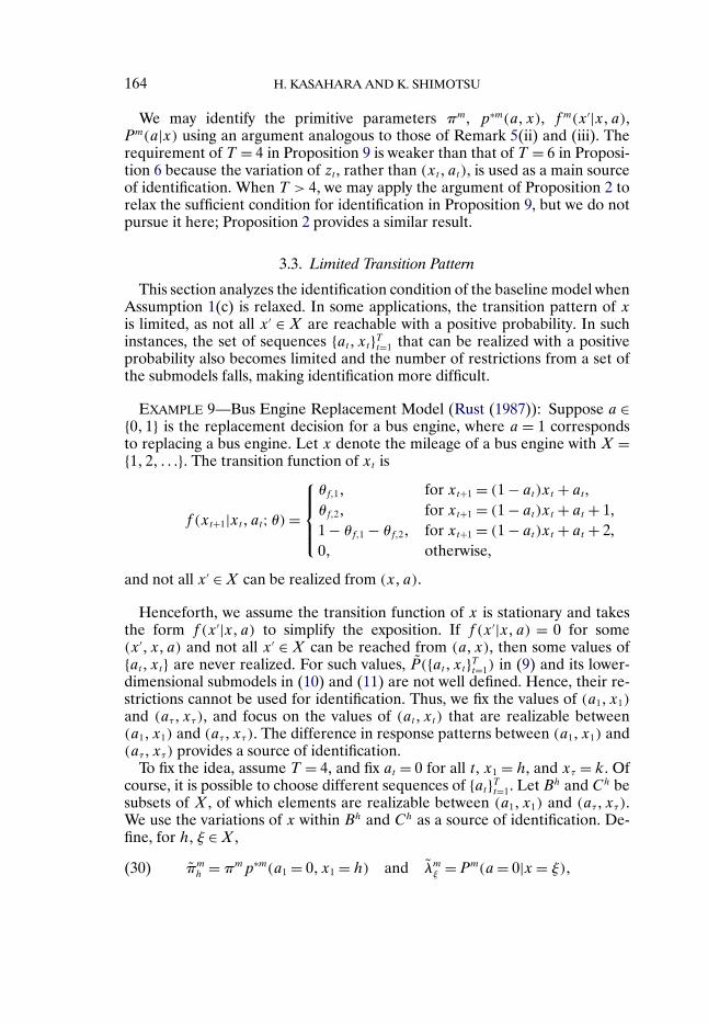
EXAMPLE 9—Bus Engine Replacement Model (Rust (1987)): Suppose a ∈{0�1} is the replacement decision for a bus engine, where a = 1 correspondsto replacing a bus engine. Let x denote the mileage of a bus engine with X ={1�2� � � �}. The transition function of xt is
f (xt+1|xt� at;θ) =
⎧⎪⎪⎨⎪⎪⎩θf�1� for xt+1 = (1 − at)xt + at ,θf�2� for xt+1 = (1 − at)xt + at + 1,1 − θf�1 − θf�2� for xt+1 = (1 − at)xt + at + 2,0� otherwise,
and not all x′ ∈X can be realized from (x�a).
Henceforth, we assume the transition function of x is stationary and takesthe form f (x′|x�a) to simplify the exposition. If f (x′|x�a) = 0 for some(x′�x�a) and not all x′ ∈ X can be reached from (a�x), then some values of{at�xt} are never realized. For such values, P({at�xt}Tt=1) in (9) and its lower-dimensional submodels in (10) and (11) are not well defined. Hence, their re-strictions cannot be used for identification. Thus, we fix the values of (a1�x1)and (aτ�xτ), and focus on the values of (at� xt) that are realizable between(a1�x1) and (aτ�xτ). The difference in response patterns between (a1�x1) and(aτ�xτ) provides a source of identification.
To fix the idea, assume T = 4, and fix at = 0 for all t, x1 = h, and xτ = k. Ofcourse, it is possible to choose different sequences of {at}Tt=1. Let Bh and Ch besubsets of X , of which elements are realizable between (a1�x1) and (aτ�xτ).We use the variations of x within Bh and Ch as a source of identification. De-fine, for h�ξ ∈X ,
πmh = πmp∗m(a1 = 0�x1 = h) and λm
ξ = Pm(a= 0|x = ξ)�(30)
MODELS OF DYNAMIC DISCRETE CHOICES 165
and Vh = diag(π1h� � � � � π
Mh ) and Dk = diag(λ1
k� � � � � λMk ). We identify Vh, Dk,
and λmξ ’s from the factorization equations corresponding to (18):
Ph = L′bVhLc and Ph
k = L′bDkVhLc�(31)
where Lb and Lc are defined analogously to L in (13), but using λmξ , and with
ξ ∈ Bh and ξ ∈ Ch, respectively. As we discuss below, we choose Bh, Ch, and kso that Ph and Ph
k are identifiable from the data.Each equation of these factorization equations (31) represents a submodel
in (9) and (10) for a sequence of at ’s and xt ’s that belongs to one of the sets
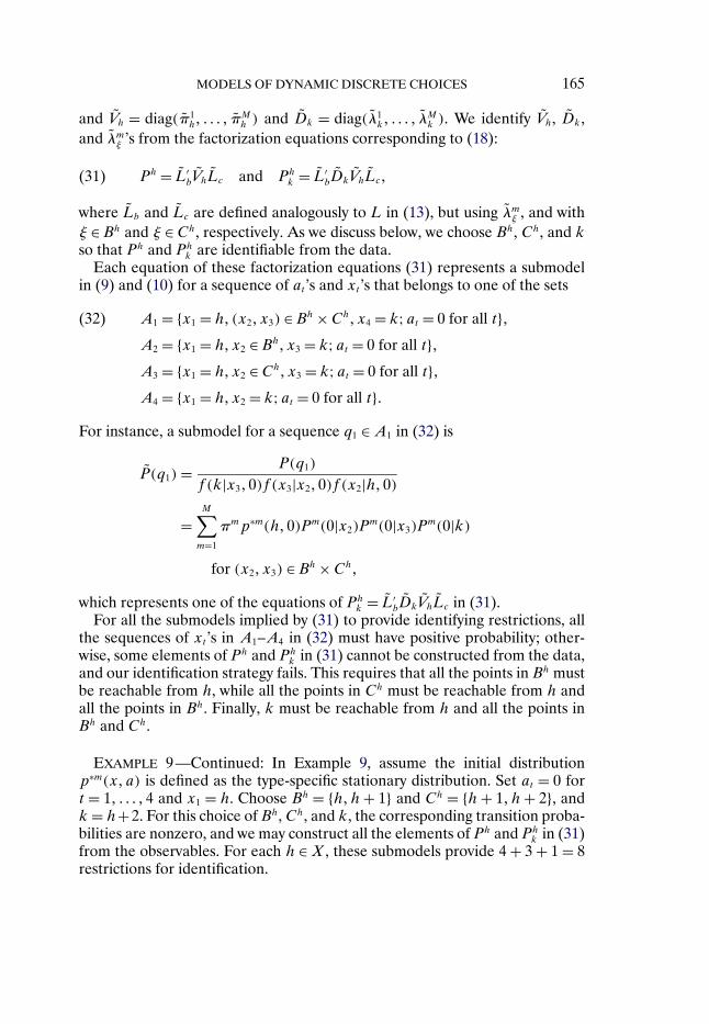
A1 = {x1 = h� (x2�x3) ∈ Bh ×Ch�x4 = k;at = 0 for all t}�(32)
A2 = {x1 = h�x2 ∈ Bh�x3 = k;at = 0 for all t}�A3 = {x1 = h�x2 ∈ Ch�x3 = k;at = 0 for all t}�A4 = {x1 = h�x2 = k;at = 0 for all t}�
For instance, a submodel for a sequence q1 ∈ A1 in (32) is
P(q1) = P(q1)
f (k|x3�0)f (x3|x2�0)f (x2|h�0)
=M∑
m=1
πmp∗m(h�0)Pm(0|x2)Pm(0|x3)P
m(0|k)
for (x2�x3) ∈ Bh ×Ch�
which represents one of the equations of Phk = L′
bDkVhLc in (31).For all the submodels implied by (31) to provide identifying restrictions, all
the sequences of xt ’s in A1–A4 in (32) must have positive probability; other-wise, some elements of Ph and Ph
k in (31) cannot be constructed from the data,and our identification strategy fails. This requires that all the points in Bh mustbe reachable from h, while all the points in Ch must be reachable from h andall the points in Bh. Finally, k must be reachable from h and all the points inBh and Ch.
EXAMPLE 9 —Continued: In Example 9, assume the initial distributionp∗m(x�a) is defined as the type-specific stationary distribution. Set at = 0 fort = 1� � � � �4 and x1 = h. Choose Bh = {h�h + 1} and Ch = {h + 1�h + 2}, andk= h+2. For this choice of Bh, Ch, and k, the corresponding transition proba-bilities are nonzero, and we may construct all the elements of Ph and Ph
k in (31)from the observables. For each h ∈ X , these submodels provide 4 + 3 + 1 = 8restrictions for identification.

166 H. KASAHARA AND K. SHIMOTSU
We now state the restrictions on Bh and Ch formally. First we develop use-ful notation. For a singleton {x} ⊂ X , let Γ (a� {x}) = {x′ ∈ X : f (x′|x�a) > 0}denote a set of x′ ∈ X that can be reached from (a�x) in the next period witha positive probability. For a subset W ⊆ X , define Γ (a�W ) as the intersectionof Γ (a� {x})’s across all x’s in W :Γ (a�W )= ⋂
x∈W Γ (a� {x}).We summarize the assumptions of this subsection including the restrictions
on Bh and Ch:
ASSUMPTION 4: (a) The choice probability of at does not depend on time.(b) The choice probability of at is independent of the lagged variable (xt−1� at−1)conditional on xt . (c) Pm(a|x) > 0 for all (a�x) ∈ A × X and m = 1� � � � �M .(d) fm
t (xt |{xτ�aτ}t−1τ=1) = f (xt |xt−1� at−1) for all m. (e) h�k ∈ X , Bh and Ch sat-
isfy p∗m(a1 = 0�x1 = h) > 0 for all m, and
Bh ⊆ Γ (0� {h})� Ch ⊆ Γ (0�Bh)∩ Γ (0� {h})�{k} ⊆ Γ (0�Ch)∩ Γ (0�Bh)∩ Γ (0� {h})�
Assumption 4(a) and (b) are identical to Assumption 1(a) and (b). Assump-tion 4(c) is necessary for the submodels to be well defined. Assumption 4(d)strengthens Assumption 1(d) by imposing stationarity and a first-order Markovproperty. It may be relaxed, but doing so would add substantial notational com-plexity. Assumption 4(e) guarantees that all the sequences we consider in thesubsets in (32) have nonzero probability. Note that the choice of Ch is affectedby how Bh is chosen. If Assumption 1(c) holds, it is possible to set Bh = Ch =X .
The next proposition provides a sufficient condition for identification underAssumption 4.
PROPOSITION 10: Suppose that Assumption 4 holds T = 4, and |Bh|, |Ch| ≥M − 1. Let {ξb
1� � � � � ξbM−1} and {ξc
1� � � � � ξcM−1} be elements of Bh and Ch, respec-
tively. Define πmh and λm
ξ as in (30), and define
Lb(M×M)
=
⎡⎢⎢⎣
1 λ1ξb1
λ1ξb2
· · · λ1ξbM−1
������
���� � �
���
1 λM
ξb1λM
ξb2· · · λM
ξbM−1
⎤⎥⎥⎦ �
Lc(M×M)
=⎡⎢⎣
1 λ1ξc1
λ1ξc2
· · · λ1ξcM−1
������
���� � �
���
1 λMξc1
λMξc2
· · · λMξcM−1
⎤⎥⎦ �
Suppose that Lb and Lc are nonsingular for some {ξb1� � � � � ξ
bM−1} and {ξc
1� � � � �
ξcM−1}, and that λm
k > 0 for all m and λmk = λn
k for any m = n. Then {πmh � λ
mξ :ξ ∈
Bh ∪Ch}Mm=1 is uniquely determined from {P({at�xt}Tt=1) : {at�xt}Tt=1 ∈ (A×X)T }.
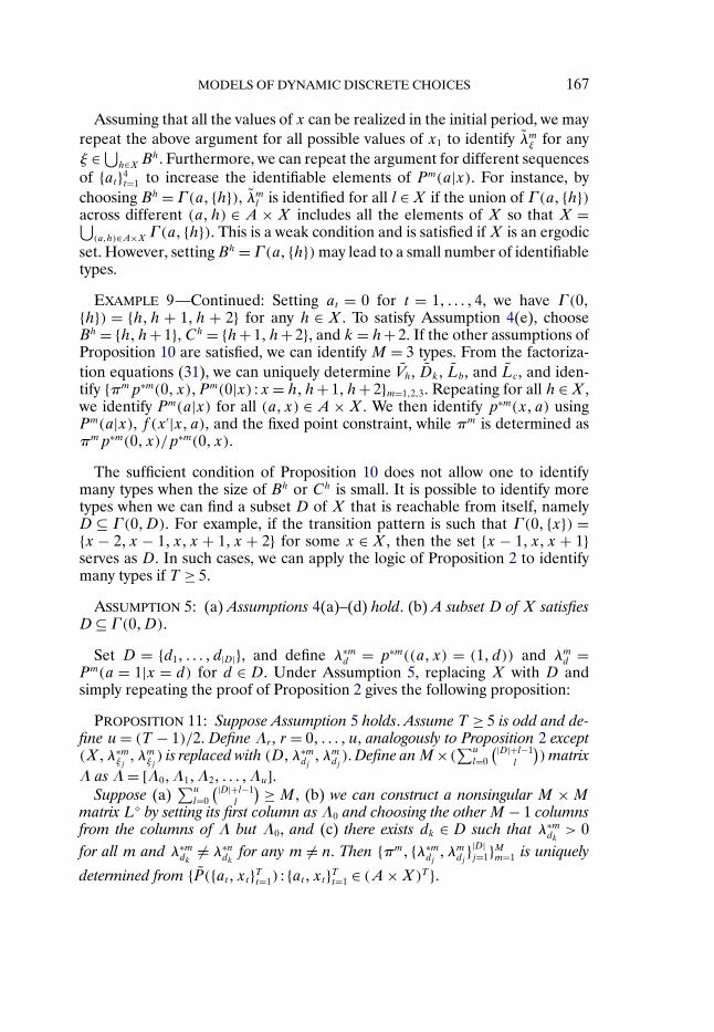
MODELS OF DYNAMIC DISCRETE CHOICES 167
Assuming that all the values of x can be realized in the initial period, we mayrepeat the above argument for all possible values of x1 to identify λm
ξ for anyξ ∈ ⋃
h∈X Bh. Furthermore, we can repeat the argument for different sequencesof {at}4
t=1 to increase the identifiable elements of Pm(a|x). For instance, bychoosing Bh = Γ (a� {h}), λm
l is identified for all l ∈ X if the union of Γ (a� {h})across different (a�h) ∈ A × X includes all the elements of X so that X =⋃
(a�h)∈A×X Γ (a� {h}). This is a weak condition and is satisfied if X is an ergodicset. However, setting Bh = Γ (a� {h}) may lead to a small number of identifiabletypes.
EXAMPLE 9—Continued: Setting at = 0 for t = 1� � � � �4, we have Γ (0�{h}) = {h�h + 1�h + 2} for any h ∈ X . To satisfy Assumption 4(e), chooseBh = {h�h+ 1}, Ch = {h+ 1�h+ 2}, and k= h+ 2. If the other assumptions ofProposition 10 are satisfied, we can identify M = 3 types. From the factoriza-tion equations (31), we can uniquely determine Vh, Dk, Lb, and Lc , and iden-tify {πmp∗m(0�x)�Pm(0|x) :x= h�h+ 1�h+ 2}m=1�2�3. Repeating for all h ∈ X ,we identify Pm(a|x) for all (a�x) ∈ A × X . We then identify p∗m(x�a) usingPm(a|x), f (x′|x�a), and the fixed point constraint, while πm is determined asπmp∗m(0�x)/p∗m(0�x).
The sufficient condition of Proposition 10 does not allow one to identifymany types when the size of Bh or Ch is small. It is possible to identify moretypes when we can find a subset D of X that is reachable from itself, namelyD ⊆ Γ (0�D). For example, if the transition pattern is such that Γ (0� {x}) ={x − 2�x − 1�x�x + 1�x + 2} for some x ∈ X , then the set {x − 1�x�x + 1}serves as D. In such cases, we can apply the logic of Proposition 2 to identifymany types if T ≥ 5.
ASSUMPTION 5: (a) Assumptions 4(a)–(d) hold. (b) A subset D of X satisfiesD ⊆ Γ (0�D).
Set D = {d1� � � � � d|D|}, and define λ∗md = p∗m((a�x) = (1� d)) and λm
d =Pm(a = 1|x = d) for d ∈ D. Under Assumption 5, replacing X with D andsimply repeating the proof of Proposition 2 gives the following proposition:
PROPOSITION 11: Suppose Assumption 5 holds. Assume T ≥ 5 is odd and de-fine u = (T − 1)/2. Define Λr , r = 0� � � � � u, analogously to Proposition 2 except(X�λ∗m
ξj�λm
ξj) is replaced with (D�λ∗m
dj�λm
dj). Define an M×(
∑u
l=0
(|D|+l−1l
)) matrix
Λ as Λ = [Λ0�Λ1�Λ2� � � � �Λu].Suppose (a)
∑u
l=0
(|D|+l−1l
) ≥ M , (b) we can construct a nonsingular M × Mmatrix L by setting its first column as Λ0 and choosing the other M − 1 columnsfrom the columns of Λ but Λ0, and (c) there exists dk ∈ D such that λ∗m
dk> 0
for all m and λ∗mdk
= λ∗ndk
for any m = n. Then {πm� {λ∗mdj�λm
dj}|D|j=1}Mm=1 is uniquely
determined from {P({at�xt}Tt=1) : {at�xt}Tt=1 ∈ (A×X)T }.
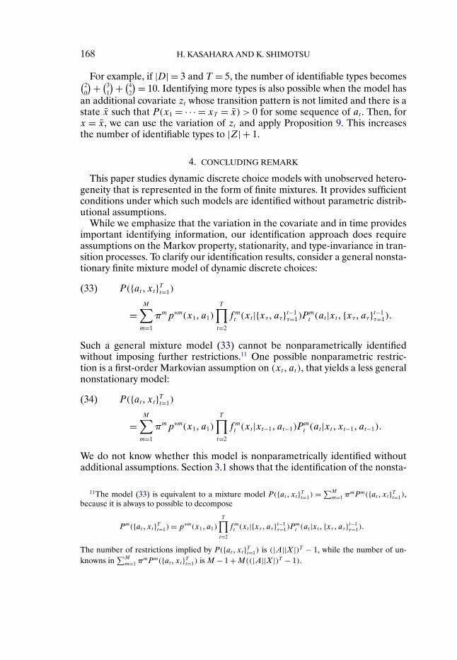
168 H. KASAHARA AND K. SHIMOTSU
For example, if |D| = 3 and T = 5, the number of identifiable types becomes(20
) + (31
) + (42
) = 10. Identifying more types is also possible when the model hasan additional covariate zt whose transition pattern is not limited and there is astate x such that P(x1 = · · · = xT = x) > 0 for some sequence of at . Then, forx = x, we can use the variation of zt and apply Proposition 9. This increasesthe number of identifiable types to |Z| + 1.
4. CONCLUDING REMARK
This paper studies dynamic discrete choice models with unobserved hetero-geneity that is represented in the form of finite mixtures. It provides sufficientconditions under which such models are identified without parametric distrib-utional assumptions.
While we emphasize that the variation in the covariate and in time providesimportant identifying information, our identification approach does requireassumptions on the Markov property, stationarity, and type-invariance in tran-sition processes. To clarify our identification results, consider a general nonsta-tionary finite mixture model of dynamic discrete choices:
P({at�xt}Tt=1)(33)
=M∑
m=1
πmp∗m(x1� a1)
T∏t=2
fmt (xt |{xτ�aτ}t−1
τ=1)Pmt (at |xt� {xτ�aτ}t−1
τ=1)�
Such a general mixture model (33) cannot be nonparametrically identifiedwithout imposing further restrictions.11 One possible nonparametric restric-tion is a first-order Markovian assumption on (xt� at), that yields a less generalnonstationary model:
P({at�xt}Tt=1)(34)
=M∑
m=1
πmp∗m(x1� a1)
T∏t=2
fmt (xt |xt−1� at−1)P
mt (at |xt�xt−1� at−1)�
We do not know whether this model is nonparametrically identified withoutadditional assumptions. Section 3.1 shows that the identification of the nonsta-
11The model (33) is equivalent to a mixture model P({at�xt}Tt=1) = ∑Mm=1 π
mPm({at�xt}Tt=1),because it is always to possible to decompose
Pm({at�xt}Tt=1)= p∗m(x1� a1)
T∏t=2
fmt (xt |{xτ�aτ}t−1
τ=1)Pmt (at |xt� {xτ�aτ}t−1
τ=1)�
The number of restrictions implied by P({at�xt}Tt=1) is (|A||X|)T − 1, while the number of un-knowns in
∑Mm=1 π
mPm({at�xt}Tt=1) is M − 1 +M((|A||X|)T − 1).
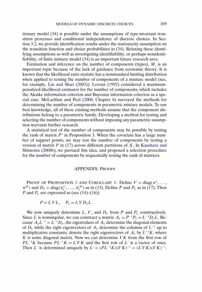
MODELS OF DYNAMIC DISCRETE CHOICES 169
tionary model (34) is possible under the assumptions of type-invariant tran-sition processes and conditional independence of discrete choices. In Sec-tion 3.2, we provide identification results under the stationarity assumption onthe transition function and choice probabilities in (34). Relaxing these identi-fying assumptions as well as investigating identifiability, or perhaps nonidenti-fiability, of finite mixture model (34) is an important future research area.
Estimation and inference on the number of components (types), M , is animportant topic because of the lack of guidance from economic theory. It isknown that the likelihood ratio statistic has a nonstandard limiting distributionwhen applied to testing the number of components of a mixture model (see,for example, Liu and Shao (2003)). Leroux (1992) considered a maximum-penalized-likelihood estimator for the number of components, which includesthe Akaike information criterion and Bayesian information criterion as a spe-cial case. McLachlan and Peel (2000, Chapter 6) surveyed the methods fordetermining the number of components in parametric mixture models. To ourbest knowledge, all of these existing methods assume that the component dis-tributions belong to a parametric family. Developing a method for testing andselecting the number of components without imposing any parametric assump-tion warrants further research.
A statistical test of the number of components may be possible by testingthe rank of matrix P∗ in Proposition 3. When the covariate has a large num-ber of support points, we may test the number of components by testing aversion of matrix P in (17) across different partitions of X . In Kasahara andShimotsu (2008b), we pursued this idea, and proposed a selection procedurefor the number of components by sequentially testing the rank of matrices.
APPENDIX: PROOFS
PROOF OF PROPOSITION 1 AND COROLLARY 1: Define V = diag(π1� � � � �πM) and Dk = diag(λ∗1
k � � � � � λ∗Mk ) as in (13). Define P and Pk as in (17). Then
P and Pk are expressed as (see (14)–(16))
P =L′V L� Pk = L′V DkL�
We now uniquely determine L, V , and Dk from P and Pk constructively.Since L is nonsingular, we can construct a matrix Ak = P−1Pk = L−1DkL. Be-cause AkL
−1 =L−1Dk, the eigenvalues of Ak determine the diagonal elementsof Dk while the right eigenvectors of Ak determine the columns of L−1 up tomultiplicative constants; denote the right eigenvectors of Ak by L−1K, whereK is some diagonal matrix. Now we can determine V K from the first row ofPL−1K because PL−1K = L′V K and the first row of L′ is a vector of ones.Then L′ is determined uniquely by L′ = (PL−1K)(V K)−1 = (L′V K)(V K)−1.
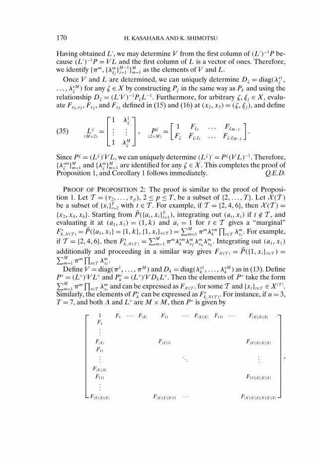
170 H. KASAHARA AND K. SHIMOTSU
Having obtained L′, we may determine V from the first column of (L′)−1P be-cause (L′)−1P = V L and the first column of L is a vector of ones. Therefore,we identify {πm� {λm
ξj}M−1j=1 }Mm=1 as the elements of V and L.
Once V and L are determined, we can uniquely determine Dζ = diag(λ∗1ζ �
� � � � λ∗Mζ ) for any ζ ∈ X by constructing Pζ in the same way as Pk and using the
relationship Dζ = (L′V )−1PζL−1. Furthermore, for arbitrary ζ�ξj ∈ X , evalu-
ate Fx2�x3 , Fx2 , and Fx3 defined in (15) and (16) at (x2�x3)= (ζ�ξj), and define
Lζ
(M×2)=
⎡⎢⎣
1 λ1ζ
������
1 λMζ
⎤⎥⎦ � Pζ
(2×M)=
[1 Fξ1 � � � FξM−1
Fζ Fζ�ξ1 � � � Fζ�ξM−1
]�(35)
Since Pζ = (Lζ)′V L, we can uniquely determine (Lζ)′ = Pζ(V L)−1. Therefore,{λ∗m
ζ }Mm=1 and {λmζ }Mm=1 are identified for any ζ ∈ X . This completes the proof of
Proposition 1, and Corollary 1 follows immediately. Q.E.D.
PROOF OF PROPOSITION 2: The proof is similar to the proof of Proposi-tion 1. Let T = (τ2� � � � � τp), 2 ≤ p ≤ T , be a subset of {2� � � � � T }. Let X (T )be a subset of {xt}Tt=2 with t ∈ T . For example, if T = {2�4�6}, then X (T ) ={x2�x4�x6}. Starting from P({at�xt}Tt=1), integrating out (at� xt) if t /∈ T , andevaluating it at (a1�x1) = (1�k) and at = 1 for t ∈ T gives a “marginal”F∗k�X (T ) = P({a1�x1} = {1�k}� {1�xt}τ∈T ) = ∑M
m=1 πmλ∗m
k
∏t∈T λm
xt. For example,
if T = {2�4�6}, then F∗k�X (T ) = ∑M
m=1 πmλ∗m
k λmx2λmx4λmx6
. Integrating out (a1�x1)
additionally and proceeding in a similar way gives FX (T ) = P({1�xt}τ∈T ) =∑M
m=1 πm
∏t∈T λm
xt.
Define V = diag(π1� � � � �πM) and Dk = diag(λ∗1k � � � � � λ
∗Mk ) as in (13). Define
P = (L)′V L and Pk = (L)′V DkL
. Then the elements of P take the form∑M
m=1 πm
∏t∈T λm
xtand can be expressed as FX (T ) for some T and {xt}t∈T ∈X |T |.
Similarly, the elements of Pk can be expressed as F∗
k�X (T ). For instance, if u= 3,T = 7, and both Λ and L are M ×M , then P is given by
⎡⎢⎢⎢⎢⎢⎢⎢⎢⎢⎢⎢⎢⎢⎢⎣
1 F1 · · · F|X| F11 · · · F|X||X| F111 · · · F|X||X||X|F1���
F|X| F|X|11 F|X||X||X||X|F11���
� � ����
F|X||X|F111 F111|X||X||X|���
F|X||X||X| F|X||X||X|11 · · · F|X||X||X||X||X||X|
⎤⎥⎥⎥⎥⎥⎥⎥⎥⎥⎥⎥⎥⎥⎥⎦
�
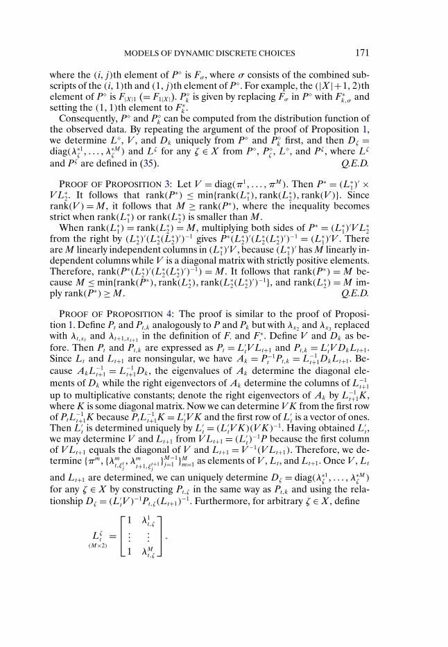
MODELS OF DYNAMIC DISCRETE CHOICES 171
where the (i� j)th element of P is Fσ , where σ consists of the combined sub-scripts of the (i�1)th and (1� j)th element of P. For example, the (|X|+1�2)thelement of P is F|X|1 (= F1|X|). P
k is given by replacing Fσ in P with F∗k�σ and
setting the (1�1)th element to F∗k .
Consequently, P and Pk can be computed from the distribution function of
the observed data. By repeating the argument of the proof of Proposition 1,we determine L, V , and Dk uniquely from P and P
k first, and then Dζ =diag(λ∗1
ζ � � � � � λ∗Mζ ) and Lζ for any ζ ∈ X from P, P
ζ , L, and Pζ , where Lζ
and Pζ are defined in (35). Q.E.D.
PROOF OF PROPOSITION 3: Let V = diag(π1� � � � �πM). Then P∗ = (L∗1)
′ ×V L∗
2. It follows that rank(P∗) ≤ min{rank(L∗1)� rank(L∗
2)� rank(V )}. Sincerank(V ) = M , it follows that M ≥ rank(P∗), where the inequality becomesstrict when rank(L∗
1) or rank(L∗2) is smaller than M .
When rank(L∗1) = rank(L∗
2) = M , multiplying both sides of P∗ = (L∗1)
′V L∗2
from the right by (L∗2)
′(L∗2(L
∗2)
′)−1 gives P∗(L∗2)
′(L∗2(L
∗2)
′)−1 = (L∗1)
′V . Thereare M linearly independent columns in (L∗
1)′V , because (L∗
1)′ has M linearly in-
dependent columns while V is a diagonal matrix with strictly positive elements.Therefore, rank(P∗(L∗
2)′(L∗
2(L∗2)
′)−1) = M . It follows that rank(P∗) = M be-cause M ≤ min{rank(P∗)� rank(L∗
2)� rank(L∗2(L
∗2)
′)−1}, and rank(L∗2) = M im-
ply rank(P∗)≥ M . Q.E.D.
PROOF OF PROPOSITION 4: The proof is similar to the proof of Proposi-tion 1. Define Pt and Pt�k analogously to P and Pk but with λx2 and λx3 replacedwith λt�xt and λt+1�xt+1 in the definition of F· and F∗
· . Define V and Dk as be-fore. Then Pt and Pt�k are expressed as Pt = L′
tV Lt+1 and Pt�k = L′tV DkLt+1.
Since Lt and Lt+1 are nonsingular, we have Ak = P−1t Pt�k = L−1
t+1DkLt+1. Be-cause AkL
−1t+1 = L−1
t+1Dk, the eigenvalues of Ak determine the diagonal ele-ments of Dk while the right eigenvectors of Ak determine the columns of L−1
t+1
up to multiplicative constants; denote the right eigenvectors of Ak by L−1t+1K,
where K is some diagonal matrix. Now we can determine V K from the first rowof PtL
−1t+1K because PtL
−1t+1K =L′
tV K and the first row of L′t is a vector of ones.
Then L′t is determined uniquely by L′
t = (L′tV K)(V K)−1. Having obtained L′
t ,we may determine V and Lt+1 from V Lt+1 = (L′
t)−1P because the first column
of V Lt+1 equals the diagonal of V and Lt+1 = V −1(V Lt+1). Therefore, we de-termine {πm� {λm
t�ξtj� λm
t+1�ξt+1j
}M−1j=1 }Mm=1 as elements of V , Lt , and Lt+1. Once V , Lt
and Lt+1 are determined, we can uniquely determine Dζ = diag(λ∗1ζ � � � � � λ
∗Mζ )
for any ζ ∈ X by constructing Pt�ζ in the same way as Pt�k and using the rela-tionship Dζ = (L′
tV )−1Pt�ζ(Lt+1)−1. Furthermore, for arbitrary ζ ∈ X , define
Lζt
(M×2)=
⎡⎢⎣
1 λ1t�ζ
������
1 λMt�ζ
⎤⎥⎦ �
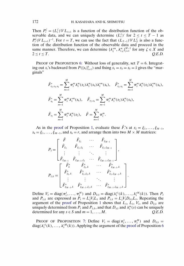
172 H. KASAHARA AND K. SHIMOTSU
Then Pζt = (Lζ
t )′V Lt+1 is a function of the distribution function of the ob-
servable data, and we can uniquely determine (Lζt )
′ for 2 ≤ t ≤ T − 1 asPζt (V Lt+1)
−1. For t = T , we can use the fact that (LT−1)′V Lζ
T is also a func-tion of the distribution function of the observable data and proceed in thesame manner. Therefore, we can determine {λ∗m
ζ �λmt�ζ}M−1
j=1 for any ζ ∈ X and2 ≤ t ≤ T . Q.E.D.
PROOF OF PROPOSITION 6: Without loss of generality, set T = 6. Integrat-ing out st ’s backward from P({st}6
t=1) and fixing s1 = s3 = s5 = s gives the “mar-ginals”
F∗s2�s4�s6
=M∑
m=1
πms λ
ms (s2)λ
ms (s4)λ
∗ms (s6)� F∗
s2�s6=
M∑m=1
πms λ
ms (s2)λ
∗ms (s6)�
F∗s6
=M∑
m=1
πms λ
∗ms (s6)� Fs2�s4 =
M∑m=1
πms λ
ms (s2)λ
ms (s4)�
Fs2 =M∑
m=1
πms λ
ms (s2)� F =
M∑m=1
πms �
As in the proof of Proposition 1, evaluate these F·’s at s2 = ξ1� � � � � ξM−1,s4 = ξ1� � � � � ξM−1, and s6 = r, and arrange them into two M ×M matrices:
Ps =
⎡⎢⎢⎢⎣
F Fξ1 · · · FξM−1
Fξ1 Fξ1�ξ1 · · · Fξ1�ξM−1
������
� � ����
FξM−1 FξM−1�ξ1 · · · FξM−1�ξM−1
⎤⎥⎥⎥⎦ �
Ps�k =
⎡⎢⎢⎢⎢⎣
F∗k F∗
ξ1�k· · · F∗
ξM−1�k
F∗ξ1�k
F∗ξ1�ξ1�k
· · · F∗ξ1�ξM−1�k
������
� � ����
F∗ξM−1�k
F∗ξM−1�ξ1�k
· · · F∗ξM−1�ξM−1�k
⎤⎥⎥⎥⎥⎦ �
Define Vs = diag(π1s � � � � �π
Ms ) and Dk|s = diag(λ∗1
s (k)� � � � � λ∗Ms (k)). Then Ps
and Ps�k are expressed as Ps = L′sVsLs and Ps�k = L′
sVsDk|sLs. Repeating theargument of the proof of Proposition 1 shows that Ls, Ls, Vs, and Dk|s areuniquely determined from Ps and Ps�k, and that Ds|s and λm
s (s) can be uniquelydetermined for any s ∈ S and m = 1� � � � �M . Q.E.D.
PROOF OF PROPOSITION 7: Define Vs = diag(π1s � � � � �π
Ms ) and Dk|s =
diag(λ∗1s (k)� � � � � λ
∗Ms (k)). Applying the argument of the proof of Proposition 6
MODELS OF DYNAMIC DISCRETE CHOICES 173
with Ls replaced by Ls , we can identify L
s , Vs, and Dk|s, and then Ds|s andλms (s) for any s ∈ S and m = 1� � � � �M . The stated result immediately follows.
Q.E.D.
PROOF OF PROPOSITION 9: The proof uses the logic of the proof of Propo-sition 6. Consider a sequence {st� zt}4
t=1 with (s1� s2� s3� s4) = (s� s� s� r) and(z1� z4) = (h�k). Summarize the value of s4 and z4 into ζ = (r�k). For(z2� z3) ∈ Z2, define Fh∗
z2�z3�ζ= ∑M
m=1 πms�hλ
ms (z2)λ
ms (z3)Q
m(r|s� k) and Fhz2�z3
=∑M
m=1 πms�hλ
ms (z2)λ
ms (z3). Define Fh∗
z2�ζ= ∑M
m=1 πms�hλ
ms (z2)Q
m(r|s� k), and defineFh∗ζ , Fh
z2, and Fh analogously to the proof of Proposition 6.
As in the proof of Proposition 6, arrange these marginals into two matricesPh and Ph
ζ . Ph and Phζ are the same as Ps and Ps�k, but F· and F∗
·�k replacedwith Fh
· and Fh∗·�ζ and subscripts are elements of Z instead of S. Define V h
s =diag(π1
s�h� � � � � πMs�h) and Dζ|s = diag(Q1(r|s� k)� � � � � QM(r|s� k)). It then follows
that Ph = L′s V
hs Ls and Ph
ζ = L′s V
hs Dζ|sLs . By repeating the argument of the
proof of Proposition 1, we can uniquely determine Ls , V hs , and Dζ|s from Ph
and Phζ , and, having determined Ls, determine D(s�z)|s for any (s� z) ∈ S × Z.
Q.E.D.
PROOF OF PROPOSITION 10: For (x2�x3) ∈ Bh × Ch and xc ∈ Bh ∪ Ch, de-fine Fh∗
x2�x3�k= ∑M
m=1 πmh λ
mx2λmx3λmk , Fh∗
xc�k= ∑M
m=1 πmh λ
mxcλmk , Fh∗
k = ∑M
m=1 πmh λ
mk ,
Fhx2�x3
= ∑M
m=1 πmh λ
mx2λmx3
, Fhxc
= ∑M
m=1 πmh λ
mxc
, and Fh = ∑M
m=1 πmh . They can be
constructed from sequentially integrating out P({at�xt}4t=1) backward and then
dividing them by a product of f (xt |xt−1�0). Note that Assumption 4(b) guar-antees f (xt |xt−1�0) > 0 for all xt and xt−1 in the subsets of X considered.
As in the proof of Proposition 1, arrange these marginals into two matricesPh and Ph
k . Ph and Phk are the same as P and Pk but F· and F∗
k�· are replacedwith Fh
· and Fh∗·�k. Define Vh = diag(π1
h� � � � � πMh ) and Dk = diag(λ1
k� � � � � λMk ). By
applying the argument in the proof of Proposition 4, we may show that Lb, Lc ,Vh, and Dk are uniquely determined from P({at�xt}4
t=1) and its marginals, andthen show that {λm
ξ }Mm=1 is determined for ξ ∈ Bh ∪Ch. Q.E.D.
REFERENCES
AGUIRREGABIRIA, V. (2006): “Another Look at the Identification of Dynamic Discrete DecisionProcesses,” Unpublished Manuscript, University of Toronto. [139]
AGUIRREGABIRIA, V., AND P. MIRA (2002): “Swapping the Nested Fixed Point Algorithm:A Class of Estimators for Discrete Markov Decision Models,” Econometrica, 70, 1519–1543.[138,160]
(2007): “Sequential Estimation of Dynamic Discrete Games,” Econometrica, 75, 1–54.[138,139,160,161]
174 H. KASAHARA AND K. SHIMOTSU
ANDERSON, T. W. (1954): “On Estimation of Parameters in Latent Structure Analysis,” Psychome-trika, 19, 1–10. [145]
BAJARI, P., AND H. HONG (2006): “Semiparametric Estimation of a Dynamic Game of Incom-plete Information,” Technical Working Paper 320, NBER. [138]
BAJARI, P., C. L. BENKARD, AND J. LEVIN (2007): “Estimating Dynamic Models of ImperfectCompetition,” Econometrica, 75, 1331–1370. [138]
BLISCHKE, W. R. (1964): “Estimating the Parameters of Mixtures of Binomial Distributions,”Journal of the American Statistical Association, 59, 510–528. [149]
BROWNING, M., AND J. CARRO (2007): “Heterogeneity and Microeconometrics Modelling,” inAdvances in Economics and Econometrics, Theory and Applications: Ninth World Congress of theEconometric Society, Vol. 3, ed. by R. Blundell, W. Newey, and T. Persson. Cambridge, U.K.:Cambridge University Press, 47–74. [141,158]
CAMERON, S. V., AND J. J. HECKMAN (1998): “Life Cycle Schooling and Dynamic Selection Bias:Models and Evidence for Five Cohorts of American Males,” Journal of Political Economy, 106,262–333. [136]
CHANDRA, S. (1977): “On the Mixtures of Probability Distributions,” Scandinavian Journal ofStatistics, 4, 105–112. [144]
CRAWFORD, G. S., AND M. SHUM (2005): “Uncertainty and Learning in Pharmaceutical De-mand,” Econometrica, 73, 1137–1173. [135]
ELBERS, C., AND G. RIDDER (1982): “True and Spurious Duration Dependence: The Identifia-bility of the Proportional Hazard Model,” Review of Economic Studies, 49, 403–409. [139]
GEWEKE, J., AND M. KEANE (2001): “Computationally Intensive Methods for Integration inEconometrics,” in Handbook of Econometrics, Vol. 5, ed. by J. Heckman and E. Leamer. Ams-terdam: North-Holland. [139]
GIBSON, W. A. (1955): “An Extension of Anderson’s Solution for the Latent Structure Equa-tions,” Psychometrika, 20, 69–73. [145]
GOWRISANKARAN, G., M. F. MITCHELL, AND A. MORO (2005): “Why Do Incumbent SenatorsWin? Evidence From a Dynamic Selection Model,” Unpublished Manuscript, Washington Uni-versity in St. Louis. [135]
HALL, P., AND X.-H. ZHOU (2003): “Nonparametric Estimation of Component Distributions ina Multivariate Mixture,” Annals of Statistics, 31, 201–224. [136,142]
HALL, P., A. NEEMAN, R. PAKYARI, AND R. ELMORE (2005): “Nonparametric Inference in Mul-tivariate Mixtures,” Biometrika, 92, 667–678. [137]
HECKMAN, J. J. (1981): “The Incidental Parameters Problem and the Problem of Initial Condi-tions in Estimating a Discrete Time-Discrete Data Stochastic Process,” in Structural Analysisof Discrete Panel Data With Econometric Applications, ed. by C. F. Manski and D. McFadden.Cambridge, MA: MIT Press, 179–195. [141]
HECKMAN, J. J., AND B. SINGER (1984): “A Method of Minimizing the Impact of DistributionalAssumptions in Econometric Models for Duration Data,” Econometrica, 52, 271–320. [136,139]
HONORÉ, B. E., AND E. TAMER (2006): “Bounds on Parameters in Panel Dynamic DiscreteChoice Models,” Econometrica, 73, 611–629. [139]
HOTZ, J., AND R. A. MILLER (1993): “Conditional Choice Probabilities and the Estimation ofDynamic Models,” Review of Economic Studies, 60, 497–529. [138,160]
HOUDE, J.-F., AND S. IMAI (2006): “Identification and 2-Step Estimation of DDC Models WithUnobserved Heterogeneity,” Unpublished Manuscript, Queen’s University. [149,150]
KASAHARA, H., AND K. SHIMOTSU (2008a): “Pseudo-Likelihood Estimation and Bootstrap Infer-ence for Structural Discrete Markov Decision Models,” Journal of Econometrics, 146, 92–106.[138,160]
(2008b): “Nonparametric Identification and Estimation of Multivariate Mixtures,” Un-published Manuscript, Queen’s University. [147,169]
KEANE, M. P., AND K. I. WOLPIN (1997): “The Career Decisions of Young Men,” Journal ofPolitical Economy, 105, 473–522. [136]
MODELS OF DYNAMIC DISCRETE CHOICES 175
KITAMURA, Y. (2004): “Nonparametric Identifiability of Finite Mixtures,” Unpublished Manu-script, Yale University. [139]
LEROUX, B. G. (1992): “Consistent Estimation of a Mixing Distribution,” Annals of Statistics, 20,1350–1360. [169]
LIU, X., AND Y. SHAO (2003): “Asymptotics for Likelihood Ratio Tests Under Loss of Identifia-bility,” Annals of Statistics, 31, 807–832. [169]
MADANSKY, A. (1960): “Determinantal Methods in Latent Class Analysis,” Psychometrika, 25,183–198. [145,148]
MAGNAC, T., AND D. THESMAR (2002): “Identifying Dynamic Discrete Decision Processes,”Econometrica, 70, 801–816. [139,147,162]
MCLACHLAN, G. J., AND D. PEEL (2000): Finite Mixture Models. New York: Wiley. [169]PAKES, A., M. OSTROVSKY, AND S. BERRY (2007): “Simple Estimators for the Parameters of Dis-
crete Dynamic Games (With Entry/Exit Examples),” RAND Journal of Economics, 38, 373–399.[138]
PESENDORFER, M., AND P. SCHMIDT-DENGLER (2008): “Asymptotic Least Squares Estimatorsfor Dynamic Games,” Review of Economic Studies, 75, 901–928. [138]
RAO, P. (1992): Identifiability in Stochastic Models. San Diego: Academic Press. [136]RIDDER, G. (1990): “The Non-Parametric Identification of Generalized Accelerated Failure-
Time Models,” Review of Economic Studies, 57, 167–181. [139]RUST, J. (1987): “Optimal Replacement of GMC Bus Engines: An Empirical Model of Harold
Zurcher,” Econometrica, 55, 999–1033. [142,164](1994): “Estimation of Dynamic Structural Models, Problems and Prospects: Discrete
Decision Processes,” in Advances in Econometrics: Sixth World Congress of the Econometric So-ciety, ed. by C. Sims. Cambridge, U.K.: Cambridge University Press, 119–170. [139,162]
TITTERINGTON, D. M., A. F. M. SMITH, AND U. E. MAKOV (1985): Statistical Analysis of FiniteMixture Distributions. New York: Wiley. [136]
VAN DEN BERG, G. J. (2001): “Duration Models: Specification, Identification and Multiple Du-rations,” in Handbook of Econometrics, Vol. 5, ed. by J. Heckman and E. Leamer. Amsterdam:North-Holland. [139]
Dept. of Economics, University of Western Ontario, London, Ontario, N6A 5C2Canada; [email protected]
andDept. of Economics, Queen’s University, 94 University Avenue, Kingston, On-
tario, K7L 3N6 Canada; [email protected].
Manuscript received October, 2006; final revision received April, 2008.


![Bayesian Nonparametric Mixture, Admixture, and ... - WUstatmath.wu.ac.at/.../Yee_Whye_Teh_WU_2015.pdf · [Gnedin & Pitman 2006, De Blasi et al 2015, Lomeli et al 2015] p(⇧](https://img.pdfslide.us/doc/110x75/5f19d9919aaddb0aa60da5bd/bayesian-nonparametric-mixture-admixture-and-gnedin-pitman-2006.jpg)