Embed Size (px)
Citation preview

EGADE® Business School TECNOLÓGICO DE MONTERREY
Hacemos constar que en la Ciudad de México, el día 12 de noviembre de 2014, el alumno:
Jorge Rosales Contreras
Sustentó el Examen de Grado en defensa de la Tesis titulada:
"Finite Gaussian Mixtures and Marketing Risk Assessment"
Presentada como requisito final para la obtención del Grado de:
DOCTORADO EN CIENCIAS FINANCIERAS
Ante la evidencia presentada en el trabajo de tesis y en este examen, el Comité Examinador, presidido por la Dra. Linda Margarita Medina Herrera ha tomado la siguiente resolución:
Lector
Dra. Linda Margarita Medina Herrera Lectora
Dr. Luis Vicente Montiel Cendejas Director del Programa Doctoral
Calle del Puente No. 222 Col. Ejidos de Huipulco. Del. Tlalpan, México D.F., C.P. 14380. Tel. +52 (55) 5483-1766
www.egade.mx

Instituto Tecnológico y de Estudios
Superiores de Monterrey
Campus Ciudad de México
Finite Gaussian Mixtures
and Market Risk Assessment
TESIS QUE PARA RECIBIR EL TÍTULO DE
DOCTORADO EN CIENCIAS FINANCIERAS
PRESENTA
Jorge Rosales Contreras ~ ~cNOLÓQCO •. DE MONTERREY
Director de tesis: Biblioteca Dr. Carlos Cuevas Covarrubias campuaCIIJdaddeMéxlco
Lectores:
Dra. Linda Margarita Medina Herrera Dr. Adán Díaz Hernández
México D.F., 12 de Noviembre de 2014

.... ·-.. , ..
.,._,, .

En cariñosa memoria de . ..
La maestra Anita
y Don Saúl
En la ansiosa espera de
Andreina Izel

Agradecimientos
A Carlos Cuevas Covarrubias por sus atinados consejos durante más de dos años de trabajo
a distancia y por no permitirme cejar en el intento.
A Linda Margarita Medina Herrera y Adán Díaz Hernández por el tiempo dedicado a la
revisión técnica de este documento y por su retroalimentación.
A José Antonio Núñez Mora por confiar en que podría concluir el doctorado en ausencia.
A mis maestros, todos, por su pequeña en lo individual pero colectivamente significativa
contribución.
A las instituciones que financiaron este proyecto:
ITESM Ciudad de México
FIDERH del Banco de México
Larrain Vial
A Rafael Flores, por su cuidadosa revisión de la redacción de este documento. Cualquier
error remanente es de mi única responsabilidad.
A los compañeros de trabajo que en estos últimos cuatro años, me permitieron ausentarme
física y mentalmente sin mayor notoriedad. Destaco a José Antonio López, Ignacio Guzmán
y Miguel Ángel González.
En el plano personal, a mis hermanos Eduardo, Gabriel, Raúl, Javier y Anita por su respaldo
incondicional y por hacerme sentir siempre en casa.
Muy particularmente a mi esposa, Nayra González Durán, por su motivación, paciencia,
comprensión y acompañamiento en los tiempos buenos igual que en los momentos de duda.
ii
Abstract
Value at Risk (VaR) is the most popular market risk measure, as it summarizes in only one figure the exposure to several risk factors. Expected Shortfall (ES) corrects its limitations and has become a standard. Both measures can be estimated under different methodologies. The most commonly used are based on the empírica} distribution of asset returns or assume that they follow a Normal distribution. This assumption is not realistic in practice dueto the skewness and excess kurtosis observed in the actual behaviour of asset returns. In this work we introduce a comprehensive methodology to evaluate risk models that includes estimation, goodness of fit, risk estimation and model validation. Following that methodology we study and apply a parametrical model based on finite Gaussian mixtures, both stationary and autocorrelated. We derive a closed-form expression for ES and implement it estimating VaR and ES for a multi-asset portfolio. Performance vs usual models (Delta-Normal and Historical Simulation) is compared through backtesting. Evidence shows that the proposed model should be considered as a serious candidate for market risk assessment. A system of early risk alerts that allows to validate models without waiting to accumulate risk and profit and loss data is proposed and used.
Resumen
El Valor en Riesgo (VaR) es la métrica de riesgo de mercado más popular, al resumir en una cifra la exposición a diversos factores de riesgo. El Déficit Esperado (ES) corrige sus limitaciones y ha ganado terreno. Ambas medidas se pueden estimar bajo distintos modelos. Los más comúnmente empleados se basan en la distribución empírica de los retornos de los activos o suponen que éstos siguen una distribución Normal. Este supuesto resulta inadecuado en la práctica debido a la elongación ( curtosis) y asimetría observados en los retornos. En el presente trabajo introducimos una metodología para evaluar modelos de riesgo que incluye estimación, bondad de ajuste, estimación de riesgo y validación del modelo. Siguiendo esa metodología estudiamos y aplicamos un modelo paramétrico basado en mixturas Gaussianas finitas, tanto estacionarias como autocorrelacionadas. Derivamos una expresión cerrada para el ES y la implementamos estimando VaR y ES para una cartera multi-activos. Comparamos los resultados vs los modelos usuales (Delta-Normal y Simulación Histórica) mediante backtesting. La evidencia muestra que el modelo estudiado es un serio candidato para la evaluación de riesgo de mercado. También se propone y usa un sistema de alertas tempranas de riesgo que permite validar modelos sin necesidad de esperar a obtener una muestra significativa de datos de riesgo y resultado.
Contents
Agradecimientos ii
Abstract iii
List of Figures vii
List of Tables viii
1 Introduction 1
2 Normality Assumption in Finance 8 2.1 Derivatives Pricing . . 9 2.2 Portfolio Optimization 9 2.3 Risk Estimation . . . . 12 2.4 Limit Distribution .. 13 2.5 Mexican Market Data 14
3 Finite Mixture Distributions 16 3.1 Introduction . . . . . . . 16
3.2 General Mixtures . . . . 17 3.2.1 Basic Definitions 17 3.2.2 Interpretation . . 18 3.2.3 Moments of Finite Mixtures . 19
3.3 Finite Gaussian Mixtures 21 3.4 ldentifiabili ty ........ 25 3.5 Estimation ......... 29
3.5.1 Method of Moments 29 3.5.2 Graphical Method 31 3.5.3 Maximum Likelihood . 32
3.6 Standard Errors . . . . . . . . 35
iv
Contents V
4 Hidden Markov Models 39 4.1 Introduction . . 39 4.2 Definitions . . . 40 4.3 Markov Chains 42 4.4 Interpretation . 44 4.5 Moments of Markov Mixtures 46 4.6 ML Estimation of finite Markov Mixtures 49
4.6.1 Known States . . 49 4.6.2 Unknown States 51
5 EM Algorithm 53 5.1 Introduction . 53 5.2 E Step ... 54 5.3 M Step .... 55 5.4 EM for GM 55 5.5 EM for HMGM 57 5.6 Discussion . . . 63 5.7 Additional Considerations 66
5.7.1 Starting Values . . 67 5.7.2 Numerical lnstabilities . 68
6 Goodness of Fit 69 6.1 Introduction . ..... 69 6.2 Q-Q Plots ... ..... 69 6.3 Kolmogorov-Smirnov. 70 6.4 Anderson-Darling. 73 6.5 Jarque-Bera. ...... 75 6.6 Discussion. ...... 76 6.7 Goodness of fit for unrestricted Gaussian Mixtures. . 79
7 Market Risk using Gaussian Mixtures 80 7.1 Introduction . . . . . . . . . 80 7.2 Portfolio Loss Distribution . 81 7.3 Market Risk Measures 83 7.4 Backtesting ....... 87 7.5 Early Alerts . . . . . . . 90 7.6 Risk Model Estimation . 93 7.7 Model Validation 95 7.8 Discussion . 97
8 Conclusions 100 8.1 Contributions . 100 8.2 General Condusions . 101
Contents vi
8.3 Future Research . . . . . . . . . . . . . . . . . . . . . . . . . . . . . . . . . . 103
A Proofs and Derivations A.l Convolution for Normal Distribution (Property 3.3). A.2 ES as Conditional Expectation (Proposition 7.4). A.3 ES for Normal Distribution ............ .
B Matlab Code B.1 VaR and ES for Gaussian Mixtures . B.2 Numerical Derivatives of Risk Measures B.3 Confidence Intervals for Risk Measures . B.4 Standard Errors for Estimators
Bibliography
106 . 106 . 107 . 108
109 . 109 . 110
. 112
. 113
115
List of Figures
2.1 Boxplots of Mexican Market Variables . . . . . . . . . . . . .
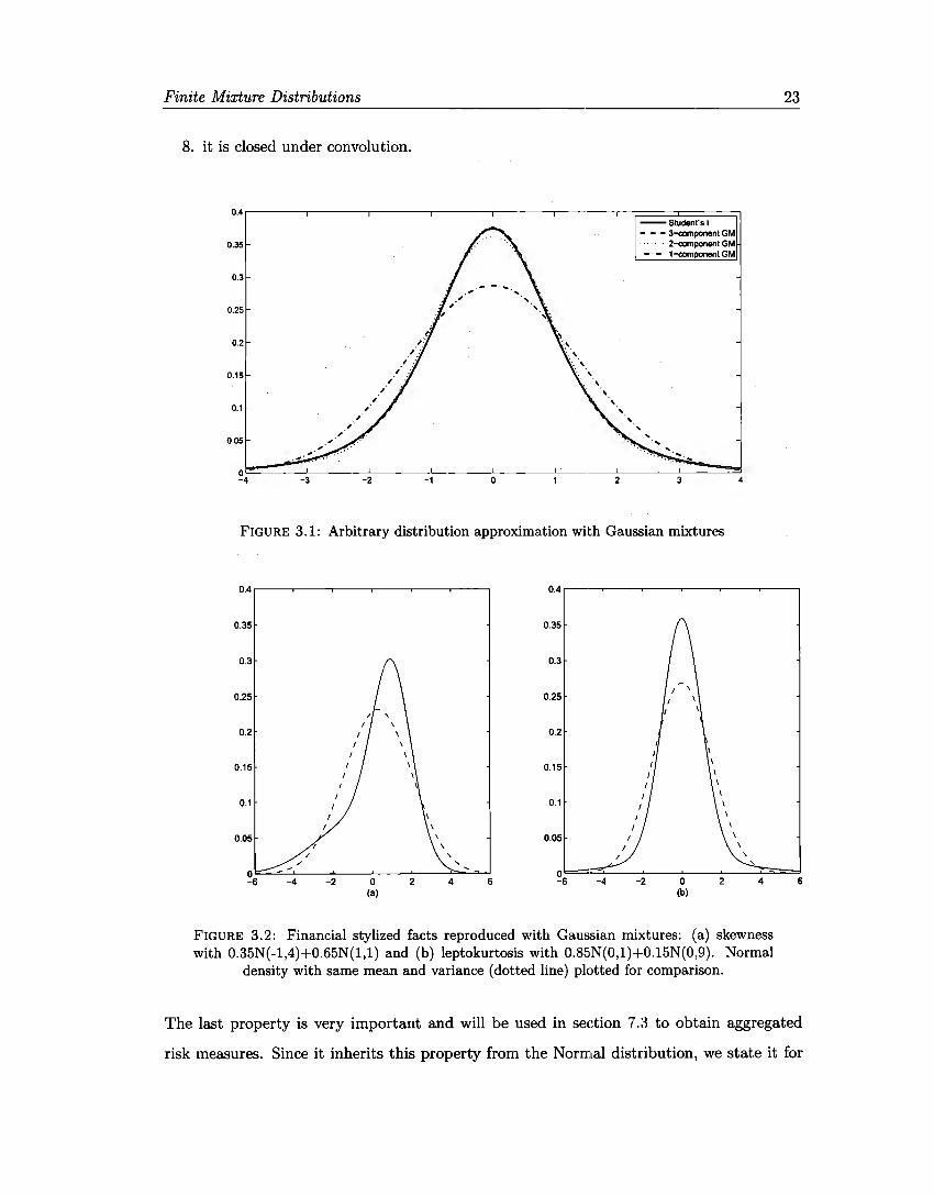
3.1 Arbitrary distribution approximation with Gaussian mixtures 3.2 Financia! stylized facts reproduced with Gaussian Mixtures 3.3 Volatility Regimes with Gaussian Mixtures
4.1 Regime Switching with Gaussian Mixtures .
5.1 Gaussian mixtures ellipsoids ........ . 5.2 Hidden Markov Gaussian mixtures ellipsoids . 5.3 Autocorrelation function. . . . . . . 5.4 Empirical Autocorrelation Function.
6.1 Normal Q-Q Plots ..... . 6.2 Gaussian Mixture Q-Q Plots 6.3 Interest rate CDF Plots . . . 6.4 Interest rate GM CDF Plots.
7.1 Backtesting VaR(99%) . 7.2 VaR(99%) Early Alerts 7.3 VaR{99%) Early Alerts 7.4 Backtesting ES{97.5%) .
Vll
14
23 23 24
45
57 64 65 66
71
72
77 78
97 98 98 99
List of Tables
2.1 EmpiricaJ Moments . . . . . . 14
5.1 Gaussian Mixture Estimators 56 5.2 Hidden Markov Gaussian Mixture Estimators 63 5.3 Hidden Markov Transition Probabilities 63 5.4 Normal Distribution Estimators . 63 5.5 Sample and Estimated Moments 65
6.1 Normality tests. . . . . . . . . 76 6.2 Gaussian Mixture K-S tests .. 76
7.1 Portfolio description. . . . . . 94 7.2 Portfolio market value and sensitivities . 94 7.3 Average VaR(99%) . 94 7.4 Average ES(97.5%) . 95 7.5 Backtesting VaR 95 7.6 Backtesting ES ... 96
viii
Chapter 1
Introduction
According to the Basel Committee, failure to capture major on- and off-balance sheet risks
. . . was a key destabalising factor during the crisis. In response to the detected shortcomings
in capital requirements, the enhanced treatment introduces a stressed Value at Risk (VaR)
capital requirement (see BCBS [6], paragraphs 11 and 12).
VaR, the most used market risk measure to estimate daily potential losses in either trading
or investment books, was not able to grasp the extent of the sub-prime mortgage market
collapse in the United States that triggered aggregated losses in market value over 130
billion (from February 2007) for firms such as Citigroup, Merrill Lynch, Morgan Stanley,
UBS, among many others.
This was mainly due to calculations based on historical simulations (heavily dependent on
sample window) or debatable assumptions whose validity was often not even verified: the
Senior Supervisors Group stated in 2008 that some firms' initial assessment o/ the true
potential losses they faced were likely skewed downward by their VaR measures' underlying
assumptions and a dependence on historical data from more benign periods [74].
Expected Shortfall (ES) is a coherent measure of risk (see Artzner et al [4]) and addresses
the VaR limitations. In particular, it is sub-additive and tells the expected potential loss in
case it exceeds VaR. Dueto its easy estimation under severa! distributional assumptions, is
has become a standard.
1
Introduction 2
In spite of the above, VaR is still the most favored metric by institutions and regulators to
monitor and control market risk (see, far instance, CNBV [19]) and the Basel Committee
uses it to set minimum capital requirements. This Committee, however, has recently agreed
to move from VaR(99%) to ES(97.5%) (see BCBS [7]).
Many financia! models assume that -or are only tractable if- the returns of financia! assets
are normally distributed. However, this assumption is usually not satisfied in practice. Em
pirical studies have shown that financia! returns frequently show lekptokurtosis or skewness,
as well as volatility clustering.
Befare applying any alternative model to estimate market risk figures, we have to quantita
tively justify that the normality assumption is not fulfilled in practice. Far that matter, we
review sorne popular -among the very many- normality test and apply them to sorne market
variables. We consider these results suffi.cient to begin the search of a more adequate model.
More in general, we postulate a methodology far testing models that includes parameter
estimation (with standard errors), goodness of fit testing, risk model estimation (again with
standard errors) and model validation. This should be the standard approach to model
testing , as it allows to identify its strengths and limitations.
However, most authors skip the calculation of standard errors and many of them avoid
testing far goodness of fit. A few even miss the now standard backtesting methodologies.
Therefare, in presenting the family of finite Gaussian Mixture clistributions as an alternative
candidate model to those most widely used in market risk estimation we fallow the proposed
methodology. Not being a well-known model, we spend two chapters studying it in detail
in the stationary and autocorrelated cases.
First we introduce the family of finite mixture distributions with arbitrary component dis
tributions. After sorne definitions, we interpret the finite mixture distribution framework
in a way that proves to be useful: we can think of the mixture distribution as an incom
plete data problem, where the component membership indicator of each sample point is not
observable.

Introduction 3
In the specific case of finite Gaussian Mixtures, we review severa! of their particular prop
erties, highlighting those that will be useful along this work. We show by means of graph
ical examples how they capture financia! stylized facts such as skewness, leptokurtosis and
volatility regimes, provide a proof of the outstanding property of closedness under con
volution and review three methods of parameter estimation; namely, a graphical method,
method of moments and maximum likelihood. For the latter we also. show how to compute
standard errors.
The family of finite Gaussian Mixture distribution is very flexible but this flexibility comes at
the price of a non-bounded likelihood function at sorne points in the border of the parameter
space, making it somewhat difficult the process of maximum likelihood estimation.
Then we relax the assumption of independence and identical distribution (iid) of the sample.
The model is therefore extended to deal with dependent data, in particular, time series that
display autocorrelation over time, captured through a stationary Markov process ( an ergodic
aperiodic Markov chain).
The reason for this election is that the so called Hidden Ma.rkov Model (HMM) is a real
istic model when the observations are collected sequentially in time and tend to cluster or
alternate between different components (or regimes, therefore the name regime switching).
Our contribution here consists in extending a result on persistence in Frühwirth-Schnatter
[34] from two states to an arbitrary number of states as long as they are classified into
two classes, or regimes. This idea can be useful to estímate the duration of a high market
volatility episode.
In an analogous way to the stationary case, we formally define the Hidden Markov Model for
finite Gaussian Mixture distributions (HMGM) and study sorne relevant properties, before
going into the estimation of a Markov switching model via maximum likelihood.
Once we have intuitively supported the pertinence of the Gaussian Mixture model ( either
stationary or autocorrelated) we can proceed to apply the first steps of the proposed method
ology, i.e., parameter estimation and standard error calculation.
Introduction 4
However, not only the likelihood function is not bounded, but also the likelihood equation
<loes not admit a closed-form solution, so that it is important to devote a whole chapter
studying the estimation algorithm under both situations: iid and autocorrelated samples.
The Expectation-Maximization (EM) algorithm is a broadly applicable approach to the
iterative computation of Maximum Likelihood Estimators in situations described as incom
plete data problems. The ideas behind the EM algorithm are natural and intuitive, so that
earlier algorithms were applied in a variety of problems. However, the seminal paper by
Dempster, Laird and Rubín [23] synthesized those ideas, provided a general formulation of
the algorithm and investigated its properties.
The basic idea of the EM algorithm is to associate the given incomplete-data problem with
a computationally tractable complete-data problem. In the Expectation step (or E-step)
we go from the observed the complete likelihood. Then the :.\1:aximization step ( or M-step)
maximizes the likelihood based on the completed data set. Starting from suitable initial
values, E-step and M-steps are iteratively repeated until convergence, according to a pre
established criteria.
We introduce the EM algorithm through the E and M-Steps and outline the algorithm for
unrestricted finite Gaussian Mixtures and Hidden Markov Ga.ussian Mixtures. In both cases
we illustrate the application of the algorithm with real data of the Mexican market and com
ment on the results. We also discuss sorne additional considerations on the implementation
of the EM algorithm.
One of the criticisms to the algorithm is that it <loes not automatically provide standard
errors. So that as a contribution we have written Matlab functions to estímate those stan
dard errors based on the empirical Information matrix as well as on the bootstrap for the
two considered models. None of the functions is currently available as a standard function
in the Statistics or Financia! toolkits in Matlab.
Continuing with the methodology we test the goodness of :fit of the Gaussian mixture to
the same data that we used to reject the normality assumption. The evidence shows that
at least the stationary version of this family of distributions is a good candidate to model

Introduction 5
the returns of the market variables considered, besides interest rates, where a high number
of components should be added to avoid rejecting the model.
The risk measures calculation ( or model estimation) step is the most popular one as there
exist vast bibliography (see below for a brief review). In orcler to be able to illustrate the
application, we first derive the Portfolio Loss Distribution following the lines of McNeil, et.
al. [57] and find the linear approximation through a loss operator that is efficient for small
changes in the underlying risk factors.
For the sake of completeness, we formally define the standard market risk measures to
be calculated on the loss distribution and obtain their estimators under four different mod
els, namely Historical Simulation, Delta-Normal, Delta-Gaussian Mixture and Delta-Hidden
Gaussian Mixture.
Our contribution here is a closed-form expression for the expected shortfall of a finite Gaus
sian mixture distribution, including its derivation. A particular case of our expression is
used in Kamaruzzaman and Isa [41], where they estimate VaR and ES for monthly and
weekly returns of a Malaysian stock index.
We propose a multi-asset-type portfolio and estimate sensibilities to risk factors, fit multi
variate Normal, stationary and autocorrelated Gaussian Mixtures distributions and estimate
market risk measures (VaR and ES) under ali models, including Historical Simulation. We
keep the Delta-Normal modelas benchmark only.
In the context of risk management, Behr and Poetter [I l] model ten European daily stock
indexes returns using hyperbolic, logF and mixtures of Gaussian distributions and conclude
that the fit of the latter is slightly superior for ali countries in almost ali subperiods. Tan and
Chu [77] model the returns of an investment portfolio using a Gaussian Mixture and estimate
VaR. They also provide a proof of closedness under convolution for Gaussian Mixtures based
on elementary calculus. Kamaruzzaman et.al. [40] fit a two--component Gaussian Mixture
to univariate monthly log-returns of three Malaysian stock indexes. In a different work [41]
they estimate VaR and ES (using an expression that is a particular case of (7.8) below)
for monthly and weekly returns of and index and find, through backtesting that it is an
Introduction 6
appropriate model. Zhang and Cheng [85] use Gaussian Mixtures with different number
of components to estímate VaR of Chinese market indexes, bound it with the VaR of the
components and link it to the behaviour of price movements and psychologies of investors.
Autocorrelated versions of Gaussian Mixutres include Alexander and Lazar [2], who use the
normal mixture GARCH(l,1) model for exchange rates. They find that a two-component
model performs better than those with three or more components and better than Student-t
GARCH models. Haas et al [36] introduce a general class of normal mixture GARCH(p,q)
models for a stock exchange index. Their models have very flexible individual variance
processes but at the cost of parsimony: their best models require from 17 to 22 parameters
to model the returns of only one index. Hardy [38] fits a regime-switching lognormal model
to monthly returns of two equity indexes and estimates VaR and ES using the payoff function
of a European put option written on an index.
Continuous versions of Gaussian Mixtures include the multivariate skew t distribution, the
multivariate normal-inverse-Gaussian distribution or the multivariate generalized hyperbolic
distribution and have been used by Lee and McLachlan [45] to model heterogeneous data
with asymmetric and heavy tail behaviour. They find that those -infinite- component densi
ties with four or more parameters can flexibly adapt to a variety of distributional shapes and
compare favourably in the estimation of VaR to Gaussian mixtures, skew normal mixtures
and shifted asymmetric Laplace mixtures, as they require a single component to accommo
date the skewness and heavy-tails in the data. Their only drawback is that the interpretation
of the parameters is not as intuitive as in the case of finite mixtures.
Severa! other distributions have been used to model risk factors returns, such as non
symmetric t distribution in Yoon and Kang [84], who find evidence suggesting that the
skewed t distribution outperformed other symmetric distributions in describing accurate
values of VaR models in Japanese financia! markets; or Generalized Error Distribution in
Theodossiou [80], who find that empirical distributions of log-returns of severa! financia!
assets at the daily, weekly, monthly, bimonthly, and quarterly frequencies possess significant
skewness and leptokurtosis and attributes them to strong high-order moment dependencies.

Introduction 7
In order to select among models, we apply the model validation step, reviewing first back
testing procedures for each risk measure and then applying them to each asset and the
portfolio. Both Gaussian Mixture models (stationary and autocorrelated) perform well at
the portfolio level at all tested confidence levels and fail in sorne instances at specific com
binations of asset and confidence level. The HMGM model <loes not seem to be superior to
the stationary version.
In summary, in this work we propose the family of finite Gaussian Mixtures as an alternative
model to fit risk factors returns distributions and estimate market risk metrics. This fam
ily preserves the parsimony of the normal model while explicitly capturing high volatility
episodes through at least one of the components. Let us highlight that we provide evidence
that it is a reasonable model for return distributions and market risk measures. We have
used the normal model and historie simulation as benchmark models dueto the spread of
their use, but we should warn the reader this is not an exhaustive or even ad-hoc model
search.
Previous versions of this work have been presented at the ASTIN, AFIR/ERM and IAALS
Colloquia, Mexico 2012 by Cuevas and Rosales [22], the Conference of the International
Federation of Classification Societies, Netherlands 2013 by Cuevas, Íñigo and Rosales [21],
and the International Finance Conference, Mexico 2014 [67], and has been published in
Rosales [68].
Chapter 2
Normality Assumption in Finance
Many models used in quantitative finance assume that the returns of financia! assets are
normally distributed. However, this fundamental assumption is usually not satisfied in
practice. Empirical studies have shown that financia! returns frequently show lekptokurtosis
or skewness ( usually negative), as well as volatility clustering. For an early analysis, see Fama
[29] who found sorne degree of leptokurtosis in every stock he analysed. He explains that,
at the time, the classic approach to this problem was to assume that the extreme values are
generated by a different mechanism than the majority of the observations. Still, he proposes
stable distributions asan alternative to account for empirically observed leptokurtosis. On
the other hand, Rosenberg [69] who found the existence of "highly significant extra-market
components of covariance among security returns", attributed lack of normality to the likely
existence of mixed normal return distributions.
In this chapter we review four common situations where either the models assume normality
or practitioners apply them under the -maybe unnecessary- assumption that the underlying
random variables follow a normal distribution. We finish introducing sorne data from the
Mexican market that will be used throughout this work and revising an apology of the usage
of the normal distribution in financia! modeling.
8
Normality Assumption in Finance 9
2.1 Derivatives Pricing
The Black and Scholes [13] model assumes that the market consists of at least one risky
asset, usually called the stock (S), and one riskless asset, usually called the money market,
cash, or bond (with constant return r). It makes several assumptions on the assets, notably
that it is a random walk (with drift, to be precise), i.e., that the instantaneous log returns
behave as a Brownian motion, and that its drift and volatility (a) are constant. If they are
time-varying, a suitably modified Black and Scholes formula can still be deduced, as long
as the volatility is not random.
The above assumptions imply that the returns follow a normal distribution and the prices
(V) follow a lognormal distribution. This allows to solve the price diffusion following differ
ential equation
élV(t, St) sªV(t, St) ! 2s2 a2V(t, St) -- V( S) _ O at + r as + 2 a as2 r t, t -
in closed form. Due to the normality assumption, the Black-Scholes framework is unable
to accommodate extreme moves in the asset returns, which practitioners hedge using out
of-the-money options. It has other limitations, such as assuming that the volatility of the
asset returns is constant. This can be overcome by adding t.he volatilit.y surface (implied
volatility as a function of strike price and maturity) as risk factor, which in turn implies that
its joint distribution with the asset returns should be normal. The same argument applies
to the interest rate.
2.2 Portfolio Optimization
Consider the allocation optimization problem
w* = argmax:S(w), wEC
Normality Assumption in Finance 10
where S is an index of satisfaction that depends on the investor's objective and C is a set
of constraints. The objective is assumed to be a linear function of the allocation w an
of the market prices vector (say M). In general it is not possible to solve this problem
analytically, and even within the realm of numerical optimization, not ali problems can be
solved. A broad class of constrained optimization problems that admit numerical solutions is
represented by convex programming: in this framework S and C are convex (see for instance
Boyd and Vandenberghe [14]).
In ali the usual formulations (the objective can be absolute wealth, relative wealth or net
profits), the investor's index of satisfaction is a functional of the distribution of the investor's
objective. In turn, the distribution of the investor's objective is in general univocally de
termined by its moments. Therefore, S can be written in terms of the -infinite number of
moments of the distribution of the objective.
The Capital Asset Pricing Model (CAPM) builds on the model of portfolio choice developed
by Markowitz (see [52] for a compilation of his work). In his model, an investor selects a
portfolio at time t - T that produces a stochastic return at t. The model assumes investors
are risk averse and, when choosing among portfolios, they care only about the mean and
variance of their one-period (of length r) investment return. As a result, investors choose
mean-variance (MV) efficient portfolios, in the sense that the portfolios 1) minimize the
variance of portfolio return, given expected return, and 2) maximize expected return, given
variance.
To say that investors only care about the first two moments of the objective means that
they neglect all higher moments, so that the MV approach is an approximation unless S is
a function of only the first two moments of the objective or the distribution of the market
M depends only on the first two moments.
Let us analyze the index of satisfaction. The only case in which it depends only on the mean
and variance of the objective is the certainty equivalent in the case of quadratic utility
1 2 u(y) = y- -y 2(
Normality Assurnption in Finance 11
as it has only two non-vanishing derivatives and the Taylor expansion consists of only three
terms. Nevertheless this utility function is not flexible enough to model investor's pref
erences, as it violates the non-satiation principie (larger values of the objective make the
investor happier), since u(y) is decreasing when y > (. There is also an additional issue
of estimation error of the utility function parameters ( ( in this case) that can adversely
affect optimality based on complicated or difficult to estimate parameters as described by
Michaud and Michaud [60).
Sharpe [75) and Lintner [50) added two key assumptions to Markovitz's model to identify a
portfolio that must be mean-variance efficient. The first of those assumptions is complete
agreement: given market clearing asset prices at t - T, investors agree on the -true- joint
distríbution of asset returns from t - T to t. See Fama and French [30) for an explanation
of the second assumption anda detailed discussion of the CAPM.
Optimized portfolios, in this framework, begin with a specific utility function that defines
satisfaction andan assumed return distribution.
Besides quadratic utility, the only other case when the MV approach is an exact solution
of the optimal allocation problem is when the distribution of the market prices M depends
only on the first two moments. Even though sorne authors claim that this property holds
for the entire family of elliptical distributions (see for instance Meucci [59), section 6.5) it is
only the case of the multivariate normal distribution.
Elliptical distributions depend on a location parameter, a scatter parameter and a charac
teristic generator that determines its tail behavior. This introduces additional parameters,
such as the degrees of freedom in the case of Student-t. Moreover, Fang, Kotz and Ng
[31) prove that a distribution is spherical (from which any elliptical can be recovered by a
linear transformation) if and only if it is equal in distribution to a continuous homoscedas
tic Gaussian mixture. The single case when this equivalence <loes not introduce additional
parameters is when the mixture is the Gaussian distribution itself (see section 3.3 below).
In summary, a MV approach, including the CAPM, provides an exact solution of the optima}
allocation problem under non-quadratic utility function only if the distribution of the market
Normality Assumption in Finance 12
is normal.
2.3 Risk Estimation
The value of an investment portfolio al time t, say Vi, is a function of time anda set of risk
factors {Zt E ffi.d): Vi= f(t, Zt) (see section 7.2 for more details).
Let us define the returns of the risk factors as Xt = Zt - Zt-r and the portfolio loss as
Lt = -(Vi - Vi-r ). Then the linear approximation to Lt+r is
(
d ) 8f(t, Zt)
Lt+r ~ - J(t, Zt) + L az- Xt-T,j , j=l J
where only the marginal returns Xt+r,j are random. If we assume that they jointly follow a
d-variate normal distribution, then Property 3.3 (section 3.3) ensures that Lt+r is itself uni
variate normal and therefore risk measures such as quantile functions (VaR) or conditional
expectations (ES) are a simple function of the parameters (see section 7.3).
However, if we are in the presence of data that has heavy tails or excess kurtosis at least, and
still fit a normal distribution for calculating VaR, then our VaR figure will underestimate
the actual risk of the portfolio. A lower estímate of VaR leads to an insufficient capital
maintained by the institution. Even if we switch the risk measure from VaR to ES, as
suggested by the Basel Committee [7], under normality VaR. at 99% confidence leve} and
ES at 97.5% confidence level are essentially the same, dueto the little mass of the normal
distribution in the tails.
The key property in this case is closedness under convolution. As opposed to the discussion
in the previous section, the family of elliptical distributions is closed under convolution and
the normal assumption is unnecessary. Moreover, this property also applies to the family of
hyperbolic distributions, of which Gaussian mixtures is a particular case. We provide the
proof of the corresponding property in section 3.3.
Normality Assumption in Finance 13
2.4 Limit Distribution
Even if we do not assume that the relevant random variable follows a normal distribution,
it is more often than not the case that the parameter we are trying to estimate is a non
linear function of that relevant random variable, making its distribution simply infeasible
to obtain. In such situation, and under certain conditions that may vary among instances,
we can use the normal as a limiting distribution.
Consider, for example, the following problem. The risk neutral valuation principle prompts
that the fair value, say f(t, Vi), of a contingent claim with maturity-payment function h(Vr)
is
ft(t, Vi) = Xt = EQ [exp (-r(T - t)) h(Vi)l$t],
where Q is the risk neutral measure and $t is the u-algebra that contains all the information
up to time t (see, for instance, Pennacchi [63], section 10.1).
When it is not possible to calculate the conditional expectation above, it is still feasible to
approximate it through the sample mean
~ 1 n ft(t, Vi)=; ¿Xt,i
j=l
from realizations of a random sample {Xt,j}, j = 1, ... ,n. A conditional version of the
central limit theorem (see Grzenda and Zieba [35]) allows us to make the statement that
the above estimator is asymptotically normal. Up to now, this is the only practica! way to
value, for instance, an American put option -with many variations, of course-.
Normality Assurnption in Finance 14
2.5 Mexican Market Data
In order to apply all the models and methodologies to be studied, we have taken a sample of
2700 daily returns, from 2003 to 2014 from representative variables of the Mexican financia!
market, namely, USDMXN foreign exchange (FX), Mexican 6-month sovereign rate (Cetes)
and Naftrac02 (an Exchange Traded Fund that replicates the behaviour of the Mexican
Stock Exchange index). A subsample of it will be used for estimation purposes and the
remaining will be kept for out-of-sample testing. At this point we present sorne exploratory
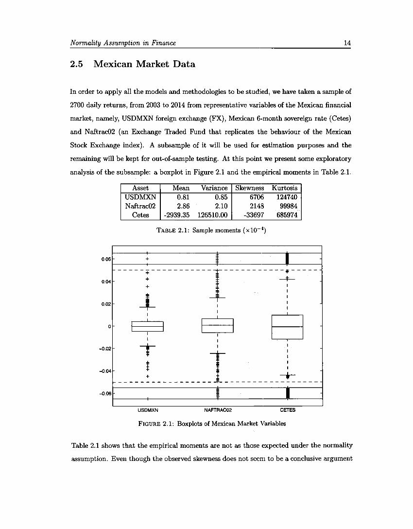
analysis of the subsample: a boxplot in Figure 2.1 and the empirical moments in Table 2.1.
Asset Mean Variance Skewness Kurtosis USDMXN 0.81 0.85 6706 124740 Naftrac02 2.86 2.10 2148 99984
Cetes -2939.35 126510.00 -33697 685974
TABLE 2.1: Sample moments {xl0- 4}
0.06 + I 1
0.04 + --4---------+-----------¡-----------~-----+ 1
1
0.02 j_ 1 :
1:1 $ a o
-0.02 T t i -0.04 .- - - - - - ~ - - - - - - - - - - -* -----------t-- - - - --0.06 1
USDMXN NAFTRAC02 CETES
FIGURE 2.1: Boxplots of Mexican Market Variables
Table 2.1 shows that the empirical moments are notas those expected under the normality
assumption. Even though the observed skewness does not seem to be a conclusive argument
Normality Assumption in Finance 15
against normality, it is not the case of empirical kurtosis, which is from 3.3 times higher than
that of the normal, for Naftrac02, to 22.9 times that benchmark for Cetes. Both features are
confirmed in the boxplots in Figure 2.1, where the boxes look symmetric around the median,
but the number of outliers ( data points located further than 1.5 times the interquantile range
from the median) is much more than expected under normality.
The simple exploratory analysis shows intuitive evidence against normality. However, the
question of whether or not the normal distribution is appropriate in financia! modeling
gives raise to endless debate. Esch (27] makes an apology of the normal distribution (not
the normal assumption) arguing through the following lines:
• although financia! returns do not follow a normal distribution they do not follow any
particular other family of distributions either,
• alternative distributions are chosen more for their convenient properties of closure
under convolution than for accurately describing returns,
• the sources of variation should be modeled rather than substituting another incorrect
distribution to directly model the data,
• parsimony is preferable to complexity for out-of-sample performance.
He also advices that models under alternative distributions may have desirable properties
in certain situations but they are often little known or not well-researched. They should be
considered when there is a good reason why they are better than the standard set of models.
In the following chapters we study, apply and test an alternative family of distributions
that encompasses the normal, allows departures from it, models such departures and still
preserves its parsimony.
Chapter 3
Finite Mixture Distributions
3.1 Introduction
In this chapter we introduce the family of finite mixture distributions with arbitrary com
ponent distributions. After sorne definitions, we interpret the finite mixture distribution
framework in a way that proves to be useful for parameter estimation purposes. We then
review moments calculation based on the moment generating function.
In the case of Gaussian Mixtures, we review several of their properties, highlighting those
that will be important later on. We provide graphical examples of how they capture financial
stylized facts such as skewness, leptokurtosis and volatility regimes. We provide a proof of
closedness under convolution based on characteristic functions in a more general context
than needed in finance. We also review three methods of parameter estimation for this
model, namely, a graphical method, method of moments and maximum likelihood. For the
latter we also show how to compute standard errors.
We mainly follow the presentation of McLachlan and Peel [53], Frühwirth-Schnatter [34]
and McNeil, Frey and Embrechts [57], but Everitt and Hand [28] and Titteringon, Smith
and Makov [81] are also excelent earlier references.
16
Finite Mixture Distributions 17
3.2 General Mixtures
3.2.1 Basic Definitions
Consider a random vector X : n ---+ !Rd where the sample space n can be discrete or
continuous. Let X be characterized by its probability density function f x(·) : JRd ---+ JR+
which is a measurable function with respect to either Lebesgue measure or a counting
measure.
Definition 3.1. Let X : n ---+ JRd be a random vector. We say that it follows a finite
(g-component) mixture distribution if its density function can be written as
9
/x(x) = L 1rj/j(x) Vx E !Rd, j=l
{3.1)
where gis a positive integer, /j : JRd---+ JR+,j = 1, ... ,g are density functions and 7rj,j =
1, ... , g are positive constants such that L}=l 7rj = l.
The number of components g will be considered fixed for our purposes, but in many ap
plications its value is another unknown parameter to be estimated. The densities /j are
called component densities, the constants 7rj are known as rnixing proportions or simply,
weights and the vector 7r1 = ( 1r1, ... , 1r 9 ) is the mixing or weight distribution. Since Ji are
densities, it is clear that the mixture density f x is well defined. Component densities are
usually assumed to come from the same parametric family, although this is not necessarily
the case. We will drop the subscript X whenever there is no confusion that f refers to the
mixture density.
Dueto linearity of the integral, Definition 3.1 may be written in terms of cumulative distri
butions functions or even characteristic functions (or moment generating functions), instead
of densities.
Finite Mixture Distributions 18
3.2.2 Interpretation
The following statistical problem where a finite mixture distribution arises in a natural way
was first noted by Feller [32] and will prove to be very useful for estimation purposes in
section 3.5.3 below.
Considera population made up of g non-overlapping subgroups, mixed at random in propor
tions 1r1, ... , 1r9 . Assume that interest líes in sorne random fea.ture X which is heterogeneous
across the groups and homogeneous within them. Due to heterogeneity, X has a different
probability distribution in each group, say Jj(Xl8), where the vector parameter 8 con
tains the specific parameters for all groups. The groups may be labeled through a discrete
indicator vector Z taking values in the set {O, 1 }gxn, where n is the sample size:
Z .. _ { 1, if Xi carne from the jth component
Ji - . O, otherwise
When sampling randomly from such a population, we may record not only X, but also the
group indicator Z. The probability of sampling X from the group labeled j (which means
Zj. = 1) is equal to 7rj, whereas conditional on knowing Zj., X is a random vector following
the distribution fi(Xl8i) with 8j being the parameter vector in group j. The joint density
f(X, Z) is given by
J(X, Z) = f(XIZ)p(Z) = fi(Xl8i)rri.
A finite mixture distribution arises if it is not possible to record the group indicator vector
Z; and only the random feature X is observable. Summing over ali possible values of Z the
marginal density f(X) is clearly given by the mixture density (3.1).
More formally, let us assume that the random vector X is defined over a sample space
n and follows a g-component mixture distribution. The intuitive interpretation above
translates into the existence of a partition {D1, n2, ... D9 } of the sample space n, where
rrj = Pr(Dj),j = 1, ... ,g. Component densities fi,j E {1, ... ,g} correspond to conditional
Finite Mixture Distributions 19
probability densities of X given Ü.j,j E {1, ... ,g} respectively. In this case, the posterior
probability of ni given a realization x of X, is
There are also many examples in practice where the components can not be identified with
exogenous groups as above, so that the components are introduced into the mixture to
allow for flexibility in modeling a heterogeneous population that is unable to be modeled by
a single component distribution. The extreme of this exercise is the nonparametric kernel
estimate of the sample density.
In this fashion, if the number of components in the mixture equals the sample size (g = n),
ali weights are 1/n, and we make Jj(x) = ik(x~xi) for some kernel density function k(-)
and bandwidth parameter h, we can think of the mixture distribution as the nonparametric
kernel estimate of a density function (see McLachlan and Pee! [53], section 1.4).
3.2.3 Moments of Finite Mixtures
For the same reason noted at the end of section 3.2.1, moments of finite mixture distributions
are easily available, as long as the moments of the component distributions exist. Indeed,
to determine the expectation of a function H(X) of the random vector X, we can write
9
E (H(X)) = 1 H(x)fx(x)dx = L 1íjEh (H(X)), n i=l
(3.2)
where Eli denotes expectation with respect to the density Í:,'.
Let H(x) = exp {t'x}, then G(t) = E (H(X)) is the moment generating function of the
random vector X, which has as many finite moments as derivatives around zero the function
G(t) has. For instance, it is easy to see that
Finite Mixture Distributions
g
µ = E(X) = G'(t =O)= L 1íjµj, j=l
provided that all the component means µ1 = fn x/j(x)dx exist.
20
(3.3)
In the univariate case, higher arder moments around zero (raw moments) are easily obtained
from the corresponding moments of the component densities:
g
µk = E(Xk) = c(k)(t =o)= L 1r1µj, j=l
(3.4)
Central moments are obtained from E (H(X)) with H(X) = (X-µ)k and Newton's binomial
formula
If k = 2, for example:
g
= L rr1E1; ((x - µj + µj - µl) j=l -t "i t. G) (µj - µ)'-' El; ((X - µj)'). (3.5)
g g
ª2 = E ((X - µ)2) = L 1íjaJ + ¿ ·rrj(µj - µ)2 j=l j=l
,, " E1r(aJ) + Var1r(µ1),
i.e., the variance of the mixture is the mean of the component variances plus the variance
of the component means, both computed with respect to the mixing distribution. In other
words, the variance of the mixture distribution captures the within component dispersion
as well as the between components dispersion. Higher central moments are:
Finite Mixture Distributions
g
cr-3E ((X - µ) 3) = cr-3 ¿ 7rj [(µj - µ) 2 + 3crJ] (µj - µ),
j=l g
cr-4E ((X - µ)4) = cr-4 L 1íj [(µj - µ)4 + 6(µj - µ) 2cr; + 3crJ].
j=l
3.3 Finite Gaussian Mixtures
21
(3.6)
(3.7)
The mixture of two univariate arbitrary normal distributions is the oldest known application
of a finite mixture distribution (Pearson [62)), where he fitted by the method of moments
this model to a dataset of crab measurements. In this section we define such mixtures and
review sorne specific properties and results to be used later on.
Definition 3.2. We say that a random vector X ~ ]Rd follows a finite Gaussian Mixture
distribution if its density function is a mixture of d-variate normal densities:
where {rri}}=l are as in the previous definition, µi E !Rd and Lj E !Rdxd are positive definite
matrices for each j = 1, ... , g.
From equation (3.2) we can obtain the characteristic function of the finite Gaussian Mixture
distribution, making H(x) = exp{it'x}, where i = v'=T:
1/Jx(t) = t 1ri exp {it' µi - ~t'Eit} J=l
{3.9)
where 1PX; (t) = exp { it' µi - ½t'Eit} is the characteristic function of the jth multivariate
normal component. This function will be useful in the proof of several properties below.

Finite Mixture Distributions 22
From {3.6), it is clear that the distribution is skewed if at least two of the component means
are distinct. From {3.7) and assuming g = 2 for illustration, if µ1 = µ 2 and cr1 #- cr2 then
the mixture distribution has fatter tails than a normal distribution.
In fact, Teicher {[78]) proves that a finite mixture of distinct Gaussian components can not
be Gaussian. More in general, it is not difficult to see that the mixture of exponential family
components with unrestricted parameters is not in the exponential family.
Besides the above, the family of finite Gaussian Mixture distributions displays the following
properties:
l. it encompasses the Normal distribution (with g = 1),
2. as noted in section 3.2.2, if g = n and under additional assumptions, we can think of
the mixture distribution as a nonparametric model,
3. for intermediate cases (1 < g < n) the mixture model can be seen as a semiparametric
model that is able to approximate any continuous distribution (see Figure 3.1),
4. its elements may be very flexible: a g-component univariate Gaussian Mixture dis
tribution can be defined using up to 3g - 1 parameters (dg(d + 3)/2 + g - 1 in the
d-variate unrestricted case), and it can be used to model a continuous distortion of
the normal -skewness, leptokurtosis, contamination models, multi-modality, etc- often
with g = 2 only (see McLachlan and Peel [53], section 1.5).
5. it has an infinite number of moments. This can be either an advantage or a limitation,
as heavy-tail1 distributions are not properly modeled.
6. it is not difficult to simulate, so it can be used in MonteCarlo or bootstrap processes.
7. it matches financia! stylized facts (as opposed to other distributions like Student-t or
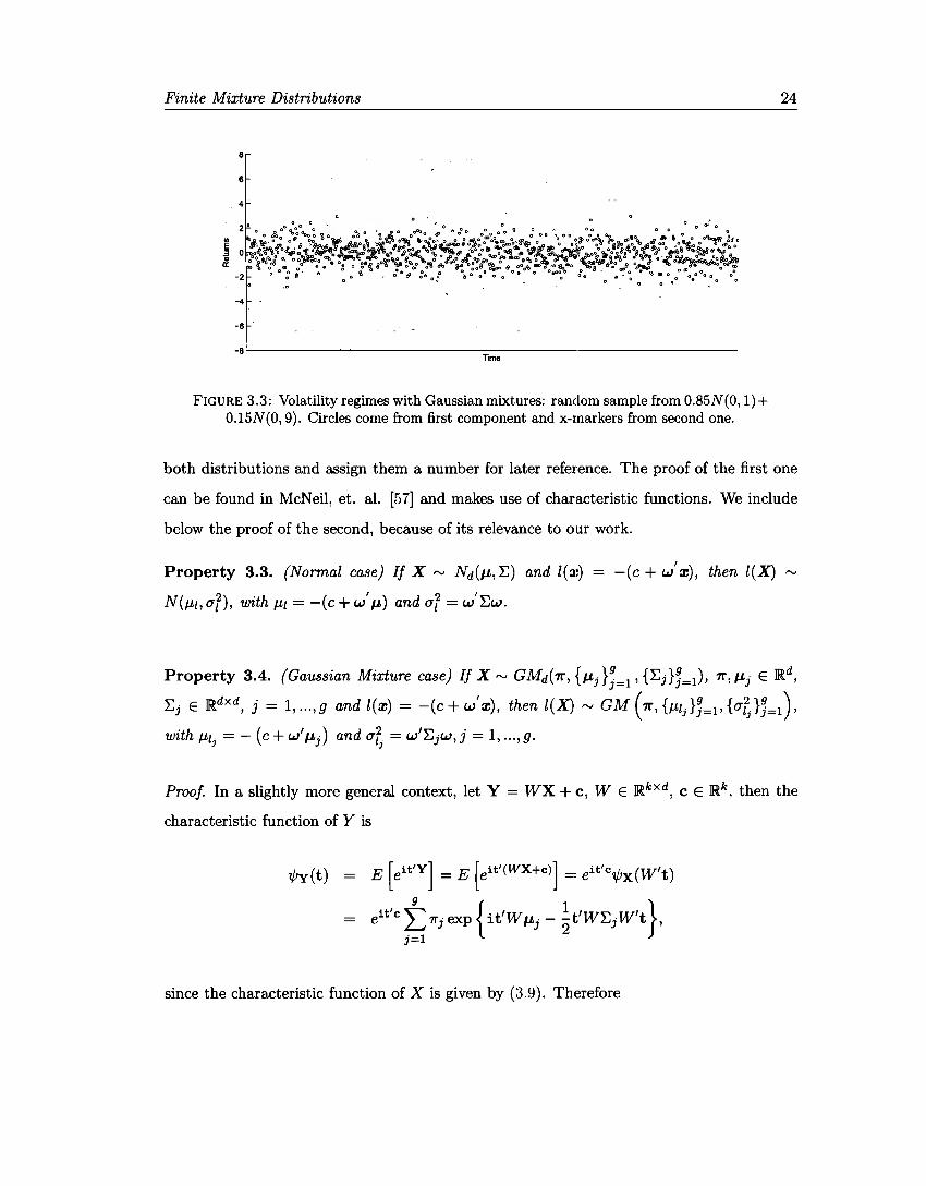
hyperbolic), such as skewness and leptokurtosis (see Figure 3.2), but markedly market
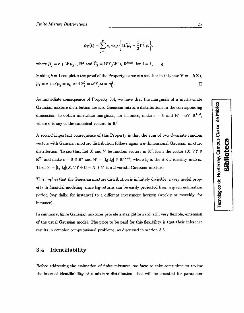
volatility regimes (see Figure 3.3).
1 For clarity, we understand that the distribution of a random variable X has a heavy right tail if limx--++oo eÁ"' P(X > x) = O. See Asmussen [5] for the definition and Klugman, et. al. [43] for a deeper discussion of tail behavior
Finite Mixture Distributions
8. it is closed under convolution.
0.4
0.35
0.3
0.25
0.2
0.15
0.1
0.05
o -4 -3 -2 -1 o 2
--Studenrs t - - - 3-component GM
· 2-component GM - · - 1-component GM
3
FIGURE 3.1: Arbitrary distribution approximation with Gaussian mixtures
0.4 0.4
0.35 0.35
0.3 0.3
0.25 0.25
0.2 0.2
0.15 0.15
0.1 0.1
o.os o.os / ' / ., ....
o -4 -2 o 2 4 6 -6 -4 -2 o 2
(a) (b)
4
\
' 4
FIGURE 3.2: Financia! stylized facts reproduced with Gaussian mixtures: (a) skewness with 0.35N(-1,4)+0.65N(l,l) and (b) leptokurtosis with 0.85N(0,1)+0.15N(0,9). Normal
density with same mean and variance ( dotted line) plotted for comparison.
23
6
The last property is very important and will be used in section 7.3 to obtain aggregated
risk measures. Since it inherits this property from the Normal distribution, we state it for
Finite Mixture Distributions
8
6
4
-4
-6
-8'------------------------------Time
FIGURE 3.3: Volatility regimes with Gaussian mixtures: random sample from 0.85N(0, 1)+ 0.15N(0, 9). Circles come from first component and x-rnarkers from second one.
24
both distributions and assign them a number for later reference. The proof of the first one
can be found in McNeil, et. al. [57] and makes use of characteristic functions. We include
below the proof of the second, because of its relevance to our work.
Property 3.3. (Normal case) lf X ,..._, Nd(µ, E) and l(:i:) = -(c + w' :i:), then l(X) ,..._,
N(µ¡, u¡), with µ¡ = -(c + w' µ) and u¡ = w 1
Ew.
Property 3.4. (Gaussian Mixture case) lf X,..._, GMd(1r, {µj };=l, {Ej}J=1), 1r, µj E JR.d,
Ej E JR.dxd, j = 1, ... ,g and l(:i:) = -(c+w':i:), then l(X) ,..._, GM(1r,{µ1JJ= 1,{u½}]=1),
with µ¡1 = - (c + w'µj) and u½= w'Ejw,j = 1, ... ,g.
Proof. In a slightly more general context, let Y= WX + e, W E JR.kxd, e E JR.k, then the
characteristic function of Y is
7h(t)
since the characteristic function of X is given by (3.9). Therefore
Finite Mixture Distributions 25
Making k = 1 completes the proof of the Property, as we can see that in this case Y= -l(X),
D
As immediate consequence of Property 3.4, we have that the marginals of a multivariate
Gaussian mixture distribution are also Gaussian mixture distributions in the corresponding
dimension: to obtain univariate marginals, for instance, make e = O and W =e'E JR.lxd,
where e is any of the canonical vectors in JR.d.
A second important consequence of this Property is that the sum of two d-variate random
vectors with Gaussian mixture distribution follows again a d-dimensional Gaussian mixture
distribution. To see this, Let X and V be random vectors in JR.d, form the vector (X, V)' E
JR.2d and make e= O E JR.d and W = ~d Id] E JR.dx 2d, where Id is the d x d identity matrix.
Then Y= [Id Id](X, V)'+ O= X+ V is a d-variate Gaussian mixture.
This implies that the Gaussian mixture distribution is infinitely divisible, a very useful prop
erty in financial modeling, since log-retums can be easily projected from a given estimation
period (say daily, for instance) to a differeµt investment horizon (weekly or monthly, for
instance).
In summary, finite Gaussian mixtures provide a straightforward, still very flexible, extension
of the usual Gaussian model. The price to be paid for this flexibility is that their inference
results in complex computational problems, as discussed in section 3.5.
3.4 ldentifiability
Before addressing the estimation of finite mixtures, we have to take sorne time to review
the issue of identifiability of a mixture distribution, that will be essential for parameter
j cu
"O "O co "O ~
ü 11) ns ~ c. u E cu a ...,
0
( ·--.e ·-1: ra o l: cu
"O o u ~g o
~
Finite Mixture Distributions 26
estimation.
As an example, consider the very simple situation of a two-component homoscedastic uni
variate Gaussian mixture f(x) = 1r<J,((x - µ¡)/u) + (1 - 1r)<J,((x - µ2)/u). There is no
way to distinguish between the two different parameter vectors e~ = ( 1r, µ 1, µ2, u) and
e~ = (1 - 1r, µ2, µ1, u) as they describe the same density.
Consider, further, the case of a univariate mixture of two normal distributions with arbitrary
parameter 0 = (1r, 0) and density /(xl8). Any mixture of two normal distributions may be
written as a mixture of three normal distributions by adding a third component with weight
1r3 = O. The parameter '11 = (1r,O,0,µ3 ,u~) is clearly different from 8 but defines the same
density /(xl'11) = /(xl0).
Let us formally define identifiability and then review the three types of nonidentifiability
distinguished by Früwirth-Schnatter [34], addressing also how to overcome them.
Definition 3.5 (Identifiability). A parametric family of distributions, indexed by a param
eter 0 E 0, defined overa sample space n, is said to be identifiable if for any two parameters
01 and 02 in e,
f (xl01) = f (xl02) for almost all x E IR<=} 01 = 02.
Invariance to Component Permutation.
Nonidentifiability of a finite mixture distribution may be caused by the invariance of a
mixture distribution to relabeling the components, as first noted by Redner and Walker
[66].
Consider a mixture of two Gaussian distributions with parameter vector (1r1, 1r2, 81, 82)
where 1r1 =/= 1r2 or 81 =/: 82. Then the distribution induced by the parameter (1r2, 1r1, 82, 81)
is the same even though the parameters are clearly different.
Finite Mixture Distributions 27
For the general finite mixture distribution with g components defined in (3.1), there exist
g! equivalent ways of arranging the components. Each of them described by a permutation
of the set { 1, ... , g}.
Because of this, a finite mixture distribution is not strictly identifiable in the sense of
Definition 3.5.
Overfitting.
Considera finite mixture distribution with g components, defined in equation (3.1), where
(1r1, ... , 1r9 , 81, ... , 89 ) E 0 9 . Consider now a finite mixture distribution from the same
parametric family, howev_er, with g - l components. Crawford [20] shows that any mixture
with g - l components defines a nonidentifiability subset in the larger parameter space 0 9 ,
which corresponds to mixtures with g components, where either one component is empty or
two components are equal.
This situation if of utmost relevance when dealing with mixtures with an unknown number
of components. Due to this type of nonidentifiability, one should exercise maximum care
when fitting finite mixture distributions by starting with n(=sample size) components and
then pruning the number of components.
In the two situations above, formal identifiability is achieved by constraining the parameter
space e in such a way that the density (3.1) is assumed to be a mixture of g distinct,
nonempty components:
• An inequality condition on the component parameters avoids nonidentifiability due
to permutation of the components. For mixtures with a multivariate component pa
rameter the arder is partial and should be required to the mixing distribution 1r or
to single entries of the vectors 8i. This is not sufficient for all situations as noted by
Frühwirth-Schnatter [34] but it worked out in all the cases we dealt with.
• A strict positivity constraint on the weights avoids nonidentifiability due to empty
components.
Finite Mixture Distributions 28
General nonidentifiability.
Finite mixture distributions may remain unidentifiable, even if a formal identifiability con
straint rules out any of the nonidentifiability problems described above. A well-known
example of a nonidentifiable family is finite mixtures of uniform distributions (see, for in
stance, Everitt and Hand [28]). A second example is finite mixtures of binomial distributions
(Titterington et al. [81 ]).
Generic identifiability of finite mixtures of distributions is a class property and has to be
defined (see Yakowitz and Spragins [83]).
Definition 3.6 (Generic Identifiability). Consider two arbitrary members of the class of
finite mixture distributions T(8) with deilsity /(-18) indexed by a vector parameter 8 E 0:
g 9*
¿ 1rjT(8j) and ¿ 1rJT(8J). j=l j=l
Assume that the formal identifiability conditions discussed above are satisfied. The class of
finite mixtures of distributions T( 8) is said to be generically identifiable, if almost every
where (a.e.) equality of the mixture density functions
g 9*
L 1íj/(-l8i) = ¿ 1rJJ(-l8J) a.e. j=l j=l
implies that g = 9* and that the two mixtures are equivalent apart from re-arranging the
components.
Teicher [79] proves that many mixtures of univariate continuous densities, especially univari
ate mixtures of normals, are generically identifiable. These results are extended by Yakowitz
and Spragins [83] to various multivariate families such as multivariate mixtures of normals.
Finite Mixture Distributions 29
3.5 Estimation
Let X' = (X1, ... , Xn) be a set of independent and identically distributed (iid) random
variables following a finite Gaussian mixture distribution. As usual, we will denote with
small caps a realization of the random variables: x' = (xi, ... , Xn)- Let 81 = { 8j }, j = 1, ... , g be the vector of parameters of the component densities, where 8j = (µj, Ej )' is the
vector of parameters of the jth component, and :Ej is understood to be a} in the univariate
case. Let E>' = (-rr, 0) be the set of parameters of the finite Gaussian mixture, where
1r' = (1r1, ... , 1r9 _i) dueto the restriction in Definition 3.1.
In this section we briefly review the estimation of E> vía method of moments and a graph
ical method, to later concentrate on maximum likelihood. Other common approaches not
discussed here include minimum-distance methods and Bayesian estimation.
3.5.1 Method of Moments
The estimation of finite Gaussian mixture parameters using the method of moments dates
back to the nineteenth century (Pearson [62]). The standard approach consists of equalising
the sample moments with the theoretical ones obtained in (3.4). In the univariate case this
reads: 1 j . 9 . .
ffij = - I: xf = I: 11"iµt = µ1, j = i, ... , k. n
i=l i=l
(3.10)
Each equation is typically nonlinear in the elements of E>. The estimation procedure requires
solving the above system of k equations and r unknowns, where r is equal to the dimension
of E>. In the unrestricted case r = 3g - 1, so that if k < 3g - 1, there exist free parameters
and the problem of finding the "optimal'' solution arises. On the other hand, if k > 3g - I
there could exist no solution.
In Pearson's pioneering work he estimated the five parameters of a two-component univariate
heteroscedastic Gaussian mixture by solving a ninth-degree polynomial, which in his time
was regarded as a "heroic task" (Charlier [18]). Efficient method-of-moments estimators
Finite Mixture Distributions 30
include Lindsay [48] for univariate mixtures and Lindsay and Basak [49] for multivariate
ones.
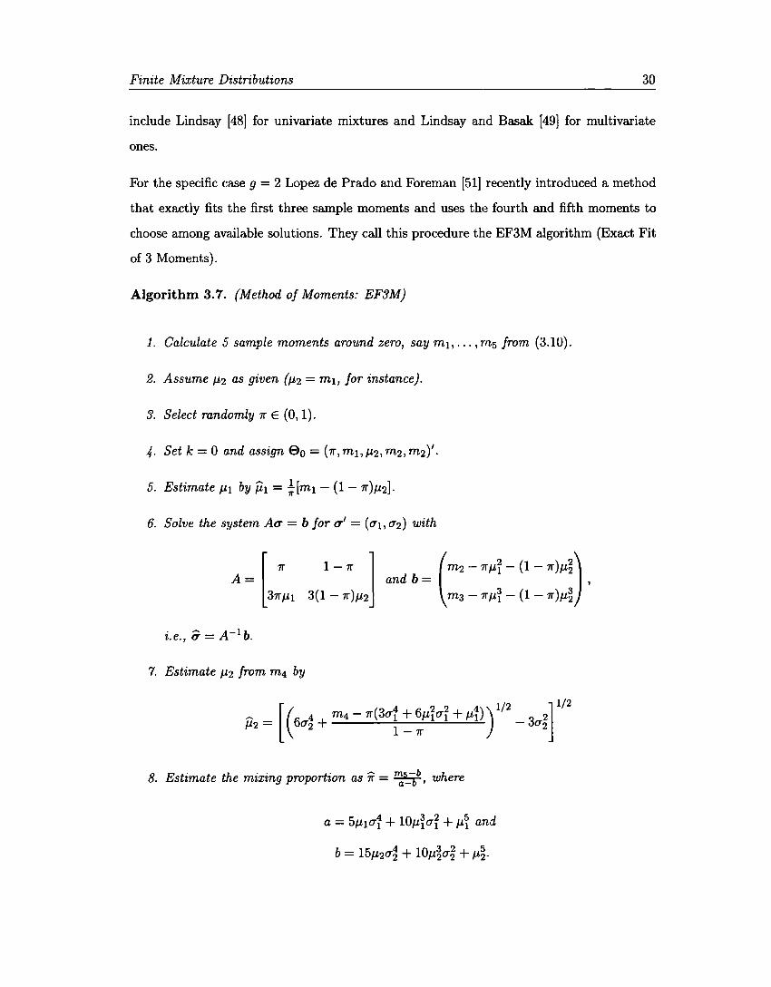
For the specific case g = 2 Lopez de Prado and Foreman [51] recently introduced a method
that exactly fits the first three sample moments and uses the fourth and fifth moments to
choose among available solutions. They call this procedure the EF3M algorithm (Exact Fit
of 3 Moments).
Algorithm 3. 7. (Method of Moments: EF3M)
1. Calculate 5 sample moments around zero, say m1, ... , m5 from (3.10).
2. Assume µ2 as given (µ2 = m1, for instance).
3. S elect randomly 1r E ( O, 1).
4- Set k = O and assign 80 = (1r,m1,µ2,m2,m2)'.
5. Estímateµ¡ by µ1 = ¼[m1 - (1 - 1r)µ2].
6. Solve the system Au = b for u'= (cr1, cr2) with
1 - 7r ]
3(1 - 1r)µ2
· ~ A-1 b i.e., u= .
7. Estímate µ2 from m4 by
~ 6 4 m4 - 1r(3cr1 + 6µ1cr1 + µ 1 3 2
[ ( 4 2 2 4)) 1/2 l 1/
2
µ2 = CT 2 + ----'----==----..::......;=------='-"- - CT 2 1 - 7r I
8. Estímate the mixing proportion as "1r = "":i_s__--/, where
- 5 4 10 3 2 5 d a - µ 1cr1 + µ 1cr1 + µ 1 an
Finite Mixture Distributions 31
1 O. Calculate convergence criterion
11. lf error> f. for a given threshold €, add 1 to k and go back to step 5, otherwise, end.
Sorne potential difficulties with the algorithm include that if µ1 and µ2 are clase to each
other or if 1r1 ~ 1 then the estimation of cr~ produces an indetermination, while if 1r1 ~ O
then µ 1 ~ oo. In addition to that, it is possible to get negative estimations for the variances
or values outside the [O, 1] interval for the mixing proportion.
Due to the calcula.tion complexities and potential difficulties as those signaled above, method
of moments estimators are not usually input as initial values in iterative estimation proce
dures such as maximum likelihood.
3.5.2 Graphical Method
In between the almost intractable method of moments and befare computers allowed the
iterative implementation of maximum likelihood, Bhattacharya [12] proposed a graphical
method to salve the problem of identifying the number of components of a univariate mixture
of normal distributions when the means are sufficiently separated, as well as to estímate the
parameters of each component.
The fundamental assumptions are: i) the components are sufficiently separated, in the sense
that for each component there exist a region where the effect of the rest of the components
is negligible, and ii) the class interval is sufficiently small. The rationale behind the above
assumptions is that, on the one hand, the data from each class will be used to estímate
parameters of a single component and, on the other hand, the error of the approximation
depends on the length of each interval. The algorithm is as follows:
Algorithm 3.8. {Graphical Method)
Finite Mixture Distributions 32
l. Group the sample in m classes of constant length h and get middle class points (xj)
and frequencies (Yi) for each class.
2. Plot ~ log(yj) = log(yi+ 1) - log(yj) against xi (j = 1, ... , m) and look for regions
Ir (r = 1, ... , g) where the graph looks like a negative-slope straight line segment.
3. The number of identified line segments (g) is the number of components.
4- Calculate the slope ( tan fJr) and the interception (Ar) of each line segment.
5. Calculate the parameter estimators of each component: µr = Ar + h/2, and a; =
hcot 0r - h2 /12.
6. Estímate mixing proportions as 'Trr = nr/ ¿¡=1 ni, where nr = ¿iElr yif ¿iElr Pr(xi)
and Pr(x) = cI>((x + h/2 - µr)/ar) - cI>((x - h/2 - µr)/crr)-
3.5.3 Maximum Likelihood
Assuming that the dataset is the realization of iid random variables, the log-likelihood
function of a multivariate g-component Gaussian Mixture is
(3.11)
The first hurdle that one has to take into account is that the likelihood function is un
bounded. Indeed, from the form of the density (3.8) if any of the data points Xj happens
to be equal to any of the component means µi (it <loes not have to be its own mean, i and
j can be different) while at the same time IEil -+ O, then the likelihood goes to inifinity.
So the global maximum <loes not exist and one has to content oneself with finding a local
maximum. Even in this situation, taking derivatives with respect to 'Tri, (i = 1, ... , g - 1)
and equalising to zero:
(3.12)
Finite Mixture Distributions 33
it is clear that it is not possible to obtain a close-form solution for the elements of 8.
Therefore, based on the interpretation discussed befare, we approach the problem as a
censored sample, where the complete sample is Xe = (x', z')' but the membership variable
Z .. _ { 1, if x1 carne from the ith component iJ -
O, otherwise
(i = 1, ... , g; j = 1, ... , n) is not observable. So the log-likelihood of the complete (unob
servable) sample is:
n g
log Le (8) = L L Zij log (1ri</> (x1; 0i)) j=l i=l
n g n g
= L L Zij log7ri + L L Zij log</> (x1; Oi) j=l i=l j=l i=l
n g l n 9
= L L Zij log 7ri - 2 L L Zij [dlog(27r) + log IEil + (xj - µd E¡1 (xj - µi)].
j=l i=l j=l i=l
Observe that ¿f=1 Zij = 1 for each j = 1, ... , n, therefore:
n g d log Le (8) = L L Zij log 7ri - ~ log(21r) -
j=l i=l
1 n g
- 2 LLZij [loglEil + (x1 - µi)'E¡ 1 (xj -µi)].
j=l i=l
(3.13)
Obtaining the Maximum Likelihood Estimators (MLEs) involves calculating derivatives from
equation (3.13) with respect to each parameter, equalising to zero and solving the resulting
system of equations. The derivative with respect to mixing proportions is
Finite Mixture Distributions
~logLc(E>) = t [Zij - Zgj] = O, 01íi . 1íi 1íg
J=l
34
(3.14)
for i = 1, ... ,9 -1, which is much easier to solve than (3.12). Let us first observe that this
equality holds also for i = g. Indeed, multiplying (3.14) by 7ri we obtain
n[ ] gn lgn 7íi L Zij - ;-Zgj = o {::> L L Zij = ;- L L 1íiZgj• j=1 g i=1 j=l g i=1 j=l
Interchanging the order of summation and using that ¿f=I Zij = l and ¿f=I 7ri = 1:
n l n l n
¿1 = -¿zgj =} 7f9ML = - ¿zgj· 1í n .
j=1 g j=1 J=l
Substituting this expression in equation (3.14):
n n l n
¿zij = 1íi ¿zgj = n1ri =} 1riML = - ¿zij, i = 1, ... ,g-1. 7r n.
j=1 g j=1 J=l
The process for µi and Ei is more straightforward:
n
{=> L ZijXj
j=l
l n -- ~2z--E:- 1 (x· - µ-)=O
2 L...,¿ lJ i 1 i
j=l
n
µi LZij j=l
Lj=l ZijXj
Lj=1 Zij (3.15)
For illustration purposes, regarding the estimation of the dispersion parameters let us con
sider first the univariate case (Ei = a¡):
Finite Mixture Distributions
a aa? log Le (0)
i
n
<=> a¡ ¿zij
j=l
In the multivariate case this becomes
n
¿ Zij (xi - µi) 2
j=l
Lj=I Zij (xi - µi)2
Lj=l Zij
35
(3.16)
(3.17)
As the membership variables Zij are not observed, it is necessary to replace them by their
conditional expectation given the sample, see section 5.2.
Maximising equation (3.13) given an estimation of the unobserved data and sorne starting
values 9(o) we can iteratively estímate the parameters of the distribution by means of the
EM algorithm, to be presented in detail in the following two chapters, first in the case
of iid data and then in the presence of a hidden Markov process, a specific instance of
autocorrelated data.
3.6 Standard Errors
The asymptotic covariance matrix of the MLE 8 is equal to the inverse of the expected
information matrix I(0), which can be approximated by I(É>). That is, the standard error
of É>j is given by (I-1(8))};2, j = 1, ... ,d.
Efron and Hinkley [24] provided justification to use the observed information matrix /(8)
instead of the expected information matrix I(0) evaluated at the MLE 0 = 8, in the case
of one parameter families ( d = I). Besides, the observed information matrix is usually more
convenient to use as it <loes not involve the calculation of an expectation.
Finite Mixture Distributions 36
Under the information based approach that uses the observed information matrix 1(8; x), we
need to calculate the Hessian matrix for the log-likelihood. Still, for unrestricted mixtures,
the calculation of the observed information matrix would be difficult, hence we have to
consider practica! methods for approximating it.
In the case of iid data, the expected information matrix I(E>) can be written as
I(E>) = n cove [s (X; E>) s' (X; E>)]
where
a s (x ··E>)= -log L(x ·· E>) 1 ' ae 1 '
and S (x; E>) = Lj=l s (xj; E>). Then an estimator of I(E>) is
n 1 le(E>;x) = ¿s (xj; E>) s' (xj; E>) - -S (x; E>) S' (x; E>). . n . J=l
Evaluating ate= 0MLE, Ie(0; x) reduces to
n
Ie(0; x) = L s(xj; 0)s'(xj; 0), j=l
(3.18)
since S(x; 0) = O. Meilijson [58] termed le(0; x) the empirical observed information matrix.
Therefore the observed information matrix 1(8; x) can be approximated by the empirical
matrix Ie(0; x) that only requires the gradient of the log-likelihood to be calculated and
can be expressed in terms of the gradient of the complete-data log-likelihood function.
Now, for finite mixture models, equation (3.18) reads
Finite Mixture Distributions
n o s (xj; 8) = ¿ Zij 08 [log 11"i + log /i(xj; Oj)], j = 1, ... , n.
j=l
37
It remains to obtain expressions for the elements of the score statistic s (xj; 8) in the case
of unrestricted multivariate normal components.
Let 1r = (1r1, ... ,1r9-1)' and let Ei contain the d(d + 1)/2 different elements of :Ei, (i =
1, ... , g). Then we can partition the vector parameter 8 as
8 - ( ' ' ' é1
é1
) - 1r,µ¡,.,.,µg, ... l,···, ... g
and take partial derivatives os (xi; 8) /08 for each element of the partition. From equation
(3.14) and the first equality of (3.15), we have
os (xi; 8) 011"i
os (xi; 8) oµij
= Zij Zgj . l l --- i= , ... ,g-- , 11"i 11" g
(3.19)
The derivatives with respect to the elements of the covariance matrix are taken from McLach
lan and Basford [54]:
(3.20)
where k = 1, ... , d(d + 1)/2 is the kth element of os (xi; 8) /otii and corresponds to the
(r, s) element of :Ei, E;l,(r) is the rth column of E¡- 1 and Órs == 1 <=> r = s.
In the same fashion as in estimation, the unobserved component indicator variables Zij are
to be replaced by their fitted conditional expectations, that is. following the interpretation

Finite Mixture Distributions 38
of section 3.2.2, by the posterior probabilities of component membership of the mixture
evaluated at the MLE for 0.
It should be emphasized that the sample size n has to be very large before the asymptotic
theory applies to mixture models.

Chapter 4
Hidden Markov Models
4.1 Introduction
The model studied in the previous chapter is based on the a.ssumption of iid-ness of the
sample. It can be extended to <leal with dependent data, in particular, time series that
display dependence over time. In this chapter we study a generalization of Gaussian mixtures
that allows serial correlation through a Markov chain. We follow the lines of Frühwirth
Schnatter [34].
Our contribution consists in extending a result on persistence :in Frühwirth-Schnatter [34]
from two regimes to an arbitrary number of regimes as long as they are classified into two
classes.
The dependence structure will be modeled through the unobservable state variable Zt E
{O, 1}9 where now the subscript t denotes time dependence and therefore the state variable
time series can be thought of as a discrete stochastic process.
In order to keep in mind the dependence in the sample, we will switch the notation from
{Xj}j=l to {Xt}¡=I · We can now think of the sample as a stochastic process with realizations
{xt}¡=1 taking values in a sample space n that can be either discrete or continuous. This
39
Hidden Markov Models 40
dataset is, in the same fashion as before, assumed to be dependent only on the unobservable
state variables and conditionally independent given the values of those variables:
T 'T g
f (xi, ... , xr lz1, ... , zr; 8) = II f (xt lzt; 8) = II II f (xt; 8j)z;t. t=l t=lj=l
We will, however, choose a very specific type of dependence. The assumption is that it is a
stationary Markov process ( an ergodic aperiodic Markov chain in the univariate case and a
Markov random field in higher dimensions).
The reason for this election is that the Hidden Markov Model (HMM) is a realistic model
when the observations are collected sequentially in time and tend to cluster or alternate
between different components ( or regimes, therefore the name regime switching, see section
4.4 below). For an early application in finance see Pagan and Schwert [61], Engel and
Hamilton [26] or Rydén, Terasvirta and Asbrink [71].
In the following sections we formally define the Hidden Markov Model for finite mixture
distributions and study sorne of its properties, before going into the estimation of a Markov
switching model based on a time series, using a modification of the EM algorithm.
4.2 Definitions
Let us assume that the unobservable component indicator variables {Zt}i=o forma discrete
time hidden process specified by a stationary Markov chain with state space {1, ... , g} and
transition probability matrix 1P given by:
{IP}i,j = p (Zt+l = j IZt = i) = Pij (4.1)
for i, j = 1, ... , g. Observe that each row of the transition matrix defines a conditional
distribution and therefore sums up to l. Observe also that the Markov chain in assumed
to be stationary, that is, transition probabilities among regimes are the same at ali times.
Hidden M arkov M odels 41
We will require two important conditions from the transition matrix, namely that it be
irreducible and aperiodic, see section 4.3. The initial distribution of the Markov chain is
defined by Po= (POi), (i = 1, ... , g).
Then the joint distribution of the time--dependent state indicator random vector can be
written as:
T
f (Z; iJ) = f (Z1; iJ) II f (Zt IZt-1; iJ) t=2
with
g g g
f (Z1; iJ) = IIP~1 and / (Zt IZt-1; iJ) = II rrp::t-lZit, i=l k=l i=l
where iJ = (p0 , IP) is the (g - l)(g + !)-dimensional vector of parameters of the Markov
chain.
In an analogous way to section 3.2.1 and taking into account the interpretation of section
3.2.2 we define a finite Markov mixture distribution as follows:
Definition 4.1 (finite Markov mixture distribution). Let {Zt, Xt}i=l be a joint stochastic
process where { Zt} follows a finite (g-state) irreducible and ergodic Markov chain with steady
state probabilities 7rj, j = 1, ... ,g and XtlZt = j ,.__, f(x; Oj) for each j = 1, ... ,g, then the
resulting unconditional distribution of Xt is called a finite Markov mixture distribution,
whose density function can be shown to be
g - ~ d fxt(x;0) = L.,¿ 1rjJ(x;Oj) \/x E lR. (4.2)
j=l
Formally speaking, equation ( 4.2) is not part of the definition as it can be easily derived
from the assumed properties of {Zt} and XtlZt and the Law of Total Probability:
Hidden M arkov M odels 42
g
fx1(x;8) = ¿f(xlZt =j;iJ,8j)P(Zt =j;iJ). j=l
We then identify f(xlZt = j; iJ, 8j) with f(x; 8j) and P(Zt := j; iJ) with 7rj, which proves
(4.2).
Even though equation (4.2) resembles very much equation (.3.1) it is important to notice
their conceptual difference. The g-dimensional mixing distribution 1r in ( 4.2) can be obtained
from the (g - l)(g + 1)-dimensional parameters iJ = (p0, IP), which are the true parameters
to be estimated, so that 8 = (8, iJ), while 9 = (8, 1r) for the standard model.
An important consequence of the above is that the Markov mixture distribution gives rise
to autocorrelation in the dataset, as shown below.
4.3 Markov Chains
In this section we will review in detail the two conditions to be required of a Markov cha.in
in a Hidden Markov Model, besides stationarity. Since the transition matrix 1P characterizes
the process, we will establish the properties in terms of its elements.
The first condition on 1P is that it should be irreducible. This means that the probability of
visiting any state in a finite time is positive, regardless of the initial state:
p (Zt+T = j IZt = i) = {IPT}i,j > o Vi,_j (4.3)
for sorne finite time T = Tij that depends on the pair of states (i,j).
A finite state space Markov cha.in has always an invariant probability (1r such that IP'1r = 1r).
Adding irreducibility ensures uniqueness of the invariant distribution (see for instance, Ross
[70]). Another implication of irreducibility for finite Markov chains is that all states are
recurrent (~:::;,:i Pjj = +oo "i/j) and in fact positive recurrent (finite expected time to return
to state j given that the process starts at state j).
Hidden Markov Models 43
A suffi.cient condition for irreducibility is that equation ( 4.3) is satisfied for sorne r indepen
dent of i and j. A stronger condition, but easier to verify is that all elements in ( 4.1) are
positive.
The second condition to be asked to 1P is that ali states are aperiodic. State j is said to have
period k if P}j = O whenever t is not divisible by k and k is the largest integer with this
property. A state with period 1 is said to be aperiodic. The idea of asking aperiodicity is
avoiding the difficulty that periodic Markov chains not necessarily converge to their invariant
probability. All positive recurrent and aperiodic states are called ergodic. lf all states are
ergodic, then the Markov chain itself is called ergodic and any invariant probability is called
ergodic probability.
A sufficient condition for aperiodicity is that all the elements in the main diagonal of 1P be
positive.
The reason why we asked for these conditions is that it can be shown that for any irre
ducible and ergodic Markov chain the invariant distribution is unique and corresponds to
the limiting probability distribution of the stochastic process regardless of its starting value.
This distribution is also called ergodic or stationary. Let us state this as a property.
Property 4.2 (Invariant distribution for irreducible ergodic Markov chains). Let 1P be an
irreducible ergodic Markov chain with invariant distribution -rr, then limt-HooP!j exists and
is independent of i, moreover
l. t . 1 1í1· = im P·.' J = ' ... 'g t-++oo iJ
and 1r is the unique positive solution of
1P'1r = 7r
(4.4)
As an illustration, let us consider the outstanding case g = 2. The stationary distribution
then reads:
Hidden Markov Models
11"1 P21
P12 + P21 P12
P12 + P21
44
From Pii = 1 - Pii, i, j = 1, 2, it is clear that if Pn = P22 then the steady state distribution
is uniform: 1r1 = 1r2, while Pu > P22 implies 1r1 > 1r2 and Pu < P22 means 1r1 < 1r2.
Since the steady-state distribution is independent of the initial distribution, then the set
of parameters to be estimated is 8 = (8, IP), where 8 = (01, ... , 89 ) correspond to the
component parameters and 1P to the transition matrix.
4.4 Interpretation
The interpretation of the standard model (section 3.2.2) in terms of regimes remains valid.
The Markov mixture model additionally allows for regime switching and therefore we can
explore properties regarding regime persistence and rate of switching. We can also think of
the standard model as a limiting case of the Markov model.
To make the regime switching property evident, compare Figure 4.1 below with Figure 3.3
from section 3.3. The mixing distributions and component distributions are the same in both
cases, but the former is a HMM, so it displays autocorrelation. We can see that the extreme
returns are randomly distributed in Figure 3.3 while there are clustered in certain portions
of Figure 4.1. This phenomenon is known as volatility clustering in Financia! jargon.
Suppose that we split the set of states (S) of the Markov chain into two mutually exclusive
classes: ordinary (O) and extraordinary (E) or stress. We may want to determine the rate
at which the process goes from O to E (let us call this phenomenon breakdowns), the average
length of time the process remains "ordinary" when it enters O or, more importantly, the
average length of time the process remains "stressed" when it enters E.
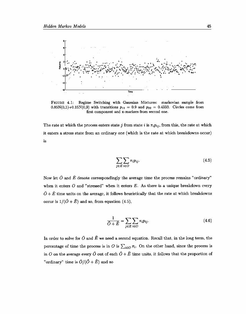
Hidden Markov Models 45
e
6
4
-4
-6'-------------------------------nma
FIGURE 4.1: Regime Switching with Gaussian Mixtures: markovian sample from 0.85N(0,1)+0.15N(0,9) with transitions Pu = 0.9 and P22 = 0.4333. Circles come from
first component and x-markers from second one.
The rate at which the process enters state j from state i is 1íi'Pij, from this, the rate at which
it enters a stress state from an ordinary one (which is the rate at which breakdowns occur)
lS
LL1íiPij· jEEiEO
(4.5)
Now let O and E denote correspondingly the average time the process remains "ordinary"
when it enters O and "stressed" when it enters E. As there is a unique breakdown every
O + E time units on the average, it follows heuristically that the rate at which breakdowns
occur is 1/(0 + E) and so, from equation (4.5),
1 E= L L 1íiPij·
jEE iEO
(4.6)
In order to solve for O and E we need a second equation. Recall that, in the long term, the
percentage of time the process is in O is I:ieO "líi- On the other hand, since the process is
in O on the average every O out of each O + E time units, it follows that the proportion of
"ordinary" time is O/ ( O + E) and so
Hidden M arkov M odels 46
(4.7)
Hence, from equations ( 4.6) and ( 4. 7)
(j = LiEO 1ri
LjEE LiEO 1riPij
E= LiEE1ri .
LjEE LiEO 1riPij (4.8)
In the case when g = 2, E for instance, reduces to 1r2/1r2P21 = 1/(1 - p22), (O reduces to
1/(1-pn)) which is equal to what Frühwirth-Schnatter [34] calls expected duration of state
j, but we have extended here to a set of states, or regimes. This feature allows Markov
mixture distributions to capture asymmetry over time.
Finally, we observe that the standard mixture models can be thought of as the limit of
the Markov mixture in the following sense. Let the transition probabilities be P(Zt =
ilZt-I = i) = P(Zt = j) = 1r;, i.e., the variables Zt199' are again iid. Then, a random
variable Xt drawn from this process follows a Markov mixture distribution with a transition
matrix 1P where ali rows are equal to 1r. In this case the autocorrelation vanishes (see
section 4.5) and Xt is equivalent to a random variable Xt that follows a standard mixture
distribution. In short, the standard mixture model is the limit of the Markov mixture model
when autocorrelation goes to zero.
4.5 Moments of Markov Mixtures
Since the unconditional distribution of a Markov mixture process Xt is the same as in (3.1)
with the stationary distribution acting as mixing distribution, a.ll the results of section 3.2.3
apply taking care of plugging in the steady-state probabilities as weights.
Hidden Markov Models 47
The random variables Xt, however, are not iid anymore and then we can study their covari
ances or, more intuitively, their autocorrelation.
Definition 4.3 (Autocorrelation function). Let {Xt}¡=1 be a stochastic process with finite
second moments. lts autocorrelation function is defined as
where µ = E ( X 1 18) and u 2 = Var ( Xt 18) are the unconditional moments and
We can write the joint unconditional density of Xt and Xt+7 as:
g
J(xt, Xt+TIS) = ¿ J(xtlZt = i, S)J(xt+T 1 Zt+T = j, 8) i,j=l
xP(Zt+T = ilZt = i, iJ)P(Zt = iliJ) g g
L f(xtl0i)1ri L f(xt+Tl0j){IP7 }i,j-i=l j=l
Taking expectations with respect to Xt and Xt+T we obtain
g g
E(xtxt+T1e) = ¿µi7riLµj{IP7
h.j-
i=l j=l
The autocorrelation function (4.9) becomes then
(4.10)
(4.11)
(4.12)
Hidden Markov Models 48
Two observations are relevant at this point. First, the autocorrelation function depends on
T only through ]PT so that persistence in the Markov chain is the parameter that determines
autocorrelation. Second, { Xt} is not a Markov process, as opposed to { Zt}
Let us consider again the special case g = 2. In this situation, Hamilton [37] found a simple
representation for ]PT in terms of the steady-state distribution and the smallest eigenvalue
of the transition matrix, namely ,\ = Pu - P21:
From this the autocorrelation function (4.12) reads
which simplifies to
(4.13)
It is clear that there is no autocorrelation if µ1 = µ2. Otherwise, the main driver of the
autocorrelation function is the structure of the transition matrix of the hidden Markov
process: if pu > P21 the process {Xt} displays positive autocorrelation and if Pu < P21 then
it displays negative autocorrelation. Recalling that P21 = 1 - P22 an equivalent criterion is
whether Pu + P22 is greater than 1 or not.
Observing that the last factor of equation {4.13) is the square of the Mahalanobis distance
between the component means, the autocorrelation function in this case can be easily ex
tended to multivariate time series as
Hidden Markov Models 49
4.6 ML Estimation of finite Markov Mixtures
Parameter estimation in HMM usually relies on maximum likelihood or Bayesian methods,
as the dependence structure magnifies the difficulties found in the iid case. The method of
moments is essentially intractable in this setting, but Quandt and Ramsey [64] provide a
solution using it.
Alternative methods of -not reviewed here- estimation include a classification likelihood ap
proach based on maximizing the complete-data likelihood function (Sclove [72]), dynamic
programming (Kim [42]) and a linear-representation-based estimator (Francq and Zakoian
[33]), where the parameters are estimated from minimizing the weighted mean-squared pre
diction error from a linear ARMA model.
We tackle the problem of maximum likelihood estimation for general Markov mixture dis
tributions by approaching it in two stages. In the first one we will assume that the state
indicator variables are known and focus our attention of the likelihood as a function of
state-specific parameters and the transition probability matrix. In the second stage we will
attack the problem of unobserved states.
4.6.1 Known States
The complete-data likelihood function for this problem is the joint density J(X, ZIE>) of
the complete data (X, Z) = {Xt, Zt};:1 given the set of parameters E> = (0, IP). This joint
sampling distribution can be written as
f(X, ZIE>) = f(XIZ, E>)p(ZIE>), (4.14)
where f(XIZ, E>) is the sampling distribution of the time series {Xt};:1 given the mem
bership variables {Zt}¿=1 , while p(ZtlE>) is the probability mass function of the sampling
distribution of this process.
Hidden M arkov M odels 50
Under the assumptions of Definition 4.1 for the state indicator process {Zt} {homogeneous
irreducible ergodic Markov chain) the distribution p(ZJ0) depends only on 1P and can be
written as:
T
p(ZJIP) = p(Zo) I1 p(ZtJZt-1, fll>) t=l T
= p(Zo) I1 IPzt-1,Zt t=l
g g
= p{Zo) I1 I1 ¡pi;;(Z) 1 {4.15)
i=l j=l
where we have used the notation !Pij instead of Pij to stress the dependence on the transition
matrix IP, and Nij(Z) counts the number of transitions from state Zt-1 = i to state Zt = j:
Nij(Z) = #{Zt-1 = i, Zt = j}, 'ili,j E {1, ... ,g}. {4.16)
The other factor of the likelihood {4.14) is the density of the sampling distribution of the
observed time series given the regime indicator variables. If we assume that only the current
state (or regime) influences the density /(XJZ, 0) and add the assumption (stated in section
4.1) that the time series is conditionally independent given the state variables:
T
f(XJZ, 0) = I1 /(XtJZt, 0) t=l
g
= rr rr 1(xt,ºj) j=l t:Z;t=l
where the second equality is just a rearrangement of the factors in the first product. It is
convenient to write the likelihood {4.14) in this way for estima,tion purposes as it separates
Hidden Markov Models 51
the parameter space into g factors that depend solely on state--specific parameters 0 i and a
factor that depends only on the transition matrix IP:
g g g
/(X, Zl0) = II II f(Xtl0j)p(Zo) II rr ¡piij(Z). (4.17) j=l t:Z;t=l i=lj=l
To take full advantage of this parameter space separation, we write the log-likelihood func
tion:
where
logLc(0) = logp(ZIIP)+log/(XIZ,0) g T
= logp(ZIIP) + ¿ ¿ log Íi(Xtl0j), j=lt=l
g g g T-1
logp(ZJIP) = ¿ Zjo logpoj + ¿ ¿ L ZitZj1+1 logPii· j=l i=l j=l t=l
4.6.2 Unknown States
(4.18)
(4.19)
Now let us move to the more realistic situation where the process {Zt} is not observed.
In this case we can write the Markov mixture likelihood function as a mixture over the
complete-data likelihood ( 4.14):
/(Xl0) = Ezes9
/(XJZ, 0)p(ZIIP)
= Ezes9
TIJ=1 Ilt:Z;t=I f(Xtl0i)p(Zo) Tif=1 TI}=l n»i;;(Z), (4.20)
Hidden M arkov M odels 52
where S9 = {1, ... ,gV+I is the sample space of Z. The sum in equation {4.20} is overa set
of cardinality gT+l and even for decently small values of g and T is infeasible for practica!
evaluation of the Markov mixture likelihood function.
An early solution to the problem of computing the likelihood function of a Markov mixture
model is provided by the forward-backward recursions of Baum [10], which are designed to
reconstruct a hidden Markov chain from a discrete signal observed with noise.
As already commented in the previous chapter, the ML function for Markov mixtures of
normal distributions with switching covariance matrices is not bounded. This is easy to see
by making Xt = µj for sorne j = 1, ... ,g andan arbitrary Xt- In this case, as l:Eil --t O,
the. likelihood goes to infinity. This means that we have to content ourselves with finding a
local maximum. A possible solution to this problem, however, is to bound l:Eil away from
zero.
Chapter 5
EM Algorithm
5.1 Introduction
The Expectation-Maximization algorithm or simply the EM algorithm is a broadly appli
cable approach to the iterative computation of MLEs in a variety of situations described
as incomplete data problems, where other numerical methods may turn out to be more
complicated. The ideas behind the EM algorithm are natural and intuitive, so that earlier
algorithms were applied in a variety of problems. However, the seminal paper by Demp
ster, Laird and Rubin [23] synthesized those ideas, provided a general formulation of the
algorithm and investigated its properties.
In particular, they proved that the sequence of estimators obtained by the algorithm in each
iteration produce a monotonic increasing sequence of likelihood values, therefore ensuring
convergence as long as the likelihood is bounded.
The basic idea of the EM algorithm is to associate the given incomplete-data problem
with a computationally tractable complete-data problem. The Expectation step (or E-step)
consists of completing the likelihood by replacing the unobserved data with it expected
value conditional on the sample and the current fit for the unknown parameters. Then
the Maximization step ( or M-step) maximizes the likelihood based on the completed data
53
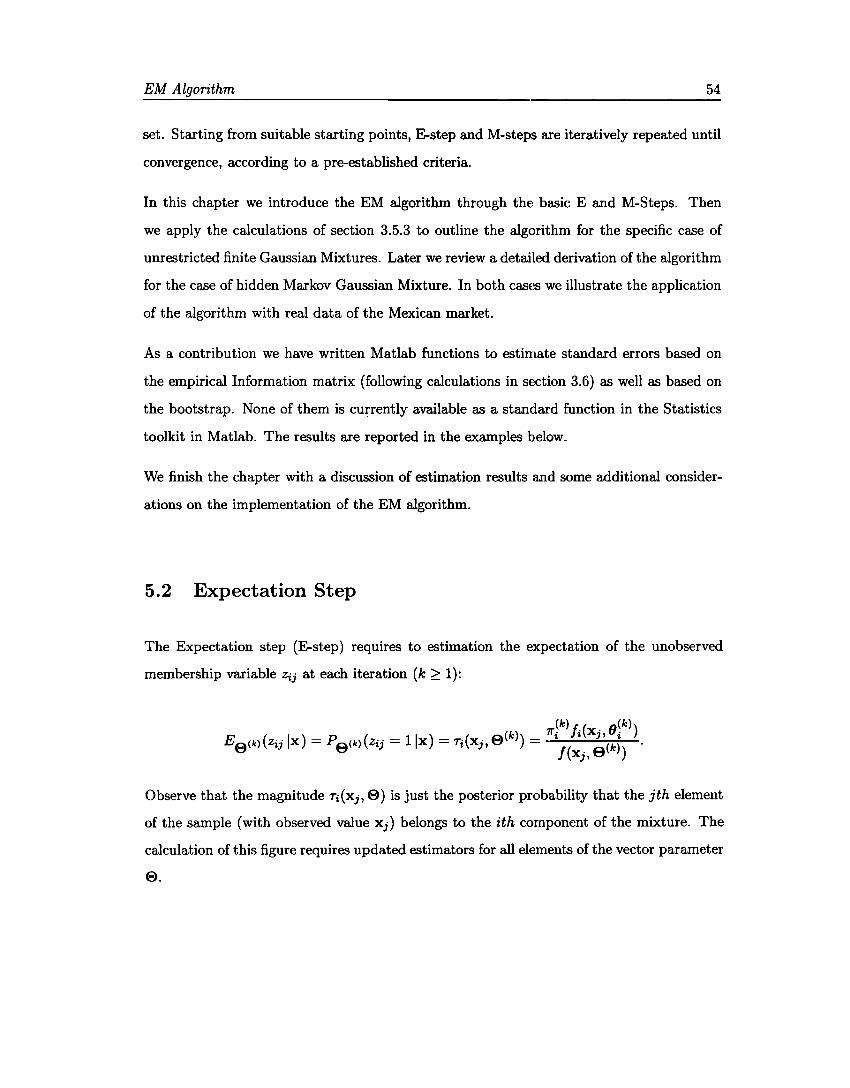
EM Algorithm 54
set. Starting from suitable starting points, E-step and M-steps are iteratively repeated until
convergence, according to a pre--established criteria.
In this chapter we introduce the EM algorithm through the basic E and M-Steps. Then
we apply the calculations of section 3.5.3 to outline the algorithm for the specific case of
unrestricted finite Gaussian Mixtures. Later we review a detailed derivation of the algorithm
for the case of hidden Markov Gaussian Mixture. In both cases we illustrate the application
of the algorithm with real data of the Mexican market.
As a contribution we have written Matlab functions to estimate standard errors based on
the empirical lnformation matrix (following calculations in section 3.6) as well as based on
the bootstrap. None of them is currently available as a standard function in the Statistics
toolkit in Matlab. The results are reported in the examples below.
We finish the chapter with a discussion of estimation results and sorne additional consider
ations on the implementation of the EM algorithm.
5.2 Expectation Step
The Expectation step (E-step) requires to estimation the expectation of the unobserved
membership variable Zij at each iteration (k ~ 1):
(k) (k) (k) 1ri fi(xj,8i )
Eo(k)(Zij lx) = Po(k)(Zij = 1 lx) = Ti(Xj,e ) = (k) . O' O' f (xj, e )
Observe that the magnitude Ti(Xj, 0) is just the posterior probability that the jth element
of the sample (with observed value Xj) belongs to the ith component of the mixture. The
calculation of this figure requires updated estimators for all elements of the vector parameter
e.
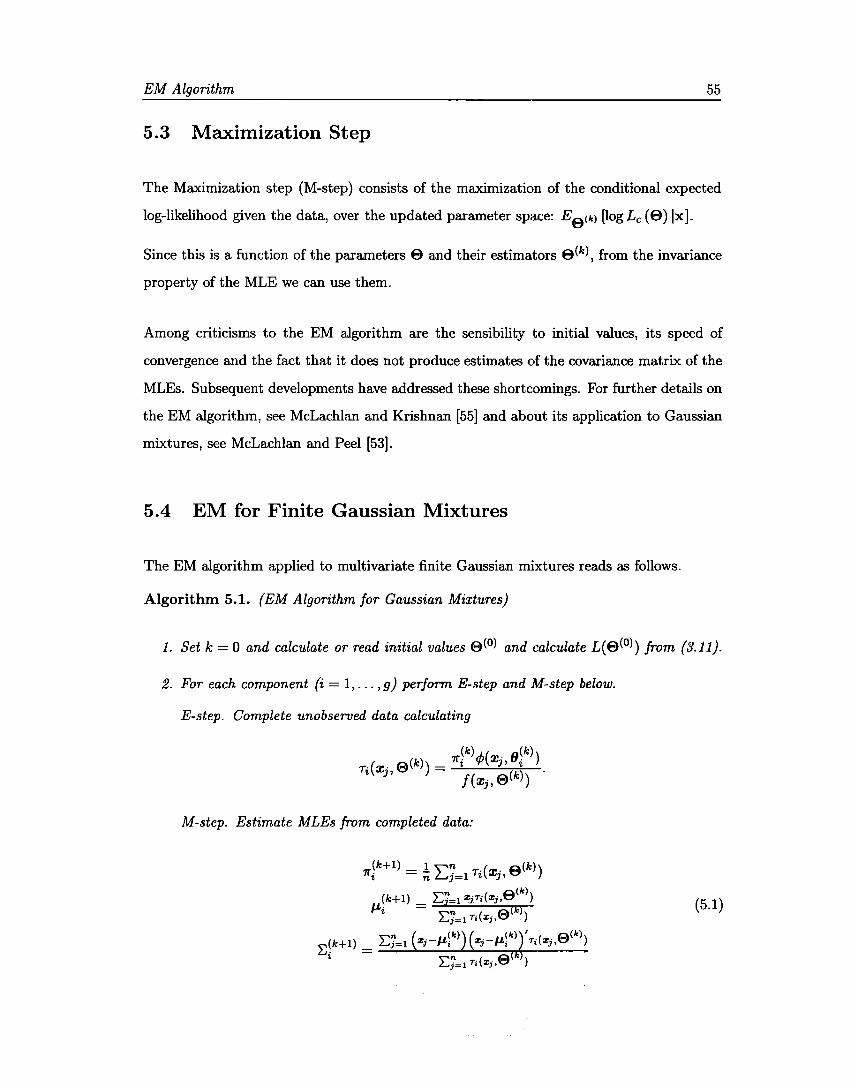
EM Algorithm 55
5 .3 Maximization Step
The Maximization step (M-step) consists of the maximization of the conditional expected
log-likelihood given the data, over the updated parameter space: E0 ckl [log Le (0) lx ].
Since this is a function of the parameters 0 and their estimators 9(k), from the invariance
property of the MLE we can use them.
Among criticisms to the EM algorithm are the sensibility to initial values, its speed of
convergence and the fa.et that it <loes not produce estimates of the covariance matrix of the
MLEs. Subsequent developments have addressed these shortcomings. For further details on
the EM algorithm, see McLachlan and Krishnan [55] and about its application to Gaussian
mixtures, see McLachlan and Peel [53].
5.4 EM for Finite Gaussian Mixtures
The EM algorithm applied to multivariate finite Gaussian mixtures reads as follows.
Algorithm 5.1. (EM Algorithm for Gaussian Mixtures)
1. Set k = O and calculate or read initial values e(o) and calculate L(e(0)) from {3.11).
2. For each component (i = 1, ... ,g) perform E-step and M-step below.
E-step. Complete unobserved data calculating
M-step. Estímate MLEs from completed data:
(k+l) _ l ~n ·( . 9(k)) 7íi - n L._¿j=l Ti XJ,
"n ( e<k)) (k+l) _ L..,j=l ZjTi Zj, µ. - (~
i Lj=l T;(z;,0 ) (5.1)
n (k)) ( (k) 1
9(k) :E~k+l) = Lj=l z;-µ; z;-µ; T;(z;, )
i Lj=l T;(z;,0 k )
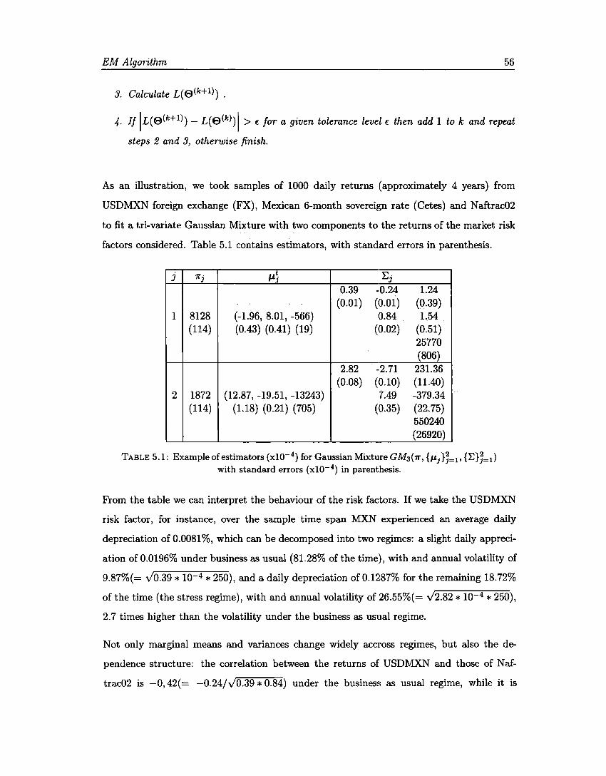
EM Algorithm 56
3. Calculate L(e(k+l}) .
4. Jf IL(e(k+l}) - L(e(k))I > f for a given tolerance level f then add 1 to k and repeat
steps 2 and 3, otherwise finish.
As an illustration, we took samples of 1000 daily returns ( approximately 4 years) from
USDMXN foreign exchange (FX), Mexican 6-month sovereign rate (Cetes) and Naftrac02
to fit a tri-variate Gaussian Mixture with two components to the returns of the market risk
factors considered. Table 5.1 contains estimators, with standard errors in parenthesis.
J 1fj µ~ Ei 0.39 -0.24 1.24
(0.01) (0.01) (0.39) 1 8128 (-1.96, 8.01, -566) 0.84 1.54
(114) (0.43) (0.41) (19) (0.02) (0.51) 25770 (806)
2.82 -2.71 231.36 (0.08) (0.10) (11.40)
2 1872 (12.87, -19.51, -13243) 7.49 -379.34 (114) (1.18) (0.21) (705) (0.35) (22.75)
550240 (26920)
TABLE 5.1: Example of estimators {xl0-4) for Gaussian Mixture GM3(1r, {µilJ=l• {E};=1 )
with standard errors (xl0- 4) in parenthesis.
From the table we can interpret the behaviour of the risk factors. lf we take the USDMXN
risk factor, for instance, over the sample time span MXN experienced an average daily
depreciation of 0.0081 %, which can be decomposed into two regimes: a slight daily appreci
ation of 0.0196% under business as usual (81.28% of the time), with and annual volatility of
9.87%(= J0.39 * 10-4 * 250), anda daily depreciation of 0.1287% for the remaining 18.72%
of the time (the stress regime), with and annual volatility of 26.55%(= J2.82 * 10-4 * 250),
2. 7 times higher than the volatility under the business as usual regime.
Not only marginal means and variances change widely accross regimes, but also the de-
pendence structure: the correlation between the returns of USDMXN and those of Naf
trac02 is -0, 42(= -0.24/J0.39 * 0.84) under the business as usual regime, while it is
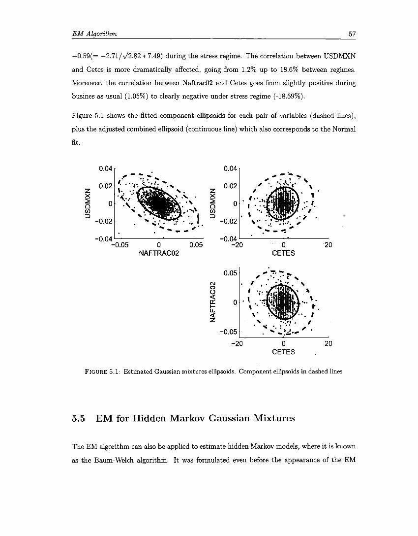
EM Algorithm 57
-0.59(= -2.71/J2.82 *-1.49) during the stress regime. The correlation between USDMXN
and Cetes is more dramatically affected, going from 1.2% up to 18.6% between regimes.
Moreover, the correlation between Naftrac02 and Cetes goes from slightly positive during
busines as usual (1.05%) to clearly negative under stress regime (-18.69%).
Figure 5.1 shows the fitted component ellipsoids for each pair of variables (dashed lines),
plus the adjusted combined ellipsoid (continuous line) which also corresponds to the Normal
fit.
0.04r 0.04 , -- .. : . .. . .....
I • • •• • ' 0.02 0.02 · · -.:·. ... . ·:. . ,
z ,. . . z X ·< .... . X ~ o :, . ~ o o . o en '
. . ..,, CI) .. . :::::, ..
. · ... ) :::::, -0.02 -0.02
;•.
-0.04 . -0.04 -0.05 o 0.05 -20 o 20
NAFTRAC02 CETES
1 . 0.05
N o (.) <( e::: o 1-LL --~ <( \, • • • • • • • • I z ' •••• , • I
-0.05 . ._; ·. : . . ~
. --. -!.:!·- . -20 o 20
CETES
FIGURE 5.1: Estimated Gaussian mixtures ellipsoids. Component ellipsoids in dashed lines
5.5 EM for Hidden Markov Gaussian Mixtures
The EM algorithm can also be applied to estimate hidden Markov models, where it is known
as the Baum-Welch algorithm. It was formulated even befare the appearance of the EM
EM Algorithm 58
(see Baum and Petrie [9], Baum and Eagon [8] and Baum, Petrie, Soules and Weiss [10] and
its convergence properties established.
The E-step can be implemented exactly, but it requires a forward and backward recursion
through the data, which is time consuming and numerically sensitive.
The M-step can be implemented in closed form, provided that the MLEs of the component
densities are available in closed form (which is the case of Gaussian components).
In what follows, the complete data are the observed data vector {X} in equation {4.18) and
the hidden component indicator vector {Z} in the same equation.
E-step.
The E-step requires the calculation of the conditional expectation of {4.18), given the ob
served data {X}:
g g g T-1 g T
E_ [10g Lc{S) IX] = ¿ Tj1 logpoj + L L L Tijt Iogpij + L L Tjt log /j{Xtl8j), e j=l i=l j=l t=l j=l t=1
(5.2)
where Tijt and Tjt denote the estimated values of the conditional probabilities defined as
Tijt = P(Zit = 1, Zjt+l = llX, 8) t = 1, ... , T - 1,
and
Tjt = P(Zjt = llX, 8) t = 1, ... , T.
From equation{5.3), we have that:
g
Tjt = L Tijt-1 t = 2, ... , T i=l
(5.3)
{5.4)
(5.5)
EM Algorithm 59
and
(5.6)
Forward-Backward Recursions.
So far we do not have available any expression to estimate the above transition probabilities.
lf we think of the realized sample as the sample path of a stochastic process, the posterior
probabilities Tijt and Tjt can be expressed in terms of the following probabilities:
ªit = f(X1, ... , Xt)P(Zjt = 1) t = 1, ... , T (5.7)
and
bit= f(Xt+I, ... , XrJZit = 1) t = T - 1, T - 2, ... , l. (5.8)
Rabiner [65] refers to the ªit as the "forward" probabilities and to the bjt as the "backward"
probabilities. lt follows that the current transition probability Tijt can be expressed in terms
of the probability of the sample path as
Tijt = .._,..g .._,..g a· p· ·J·(x · O ·)b · 1' L.,i=l L.,j=l it tJ J t, J Jt+
(5.9)
since the numerator is P(Zit = 1, Zjt+l = l)fi(x; Oj) and the denominator is f(x; O).
The following algorithm allows to estimate the posterior probabilities. The superscript (k)
refers to the iteration of the EM algorithm to be detailed shortly.
Algorithm 5.2. (Forward-Backward Recursions)
EM Algorithm 60
1. Calculate forward probabilities recursively
(k+l) (k) (k) . ªi1 =p0ifi(x1,0i )i=l, ... ,g
and g
(k+I) - ~ (k+l) (k) ·( (k) -ªit+l - ~ªit Pji Íi Xt+1,0i ) t-1, ... ,T-l.
j=l
2. Calculate backward probabilities through the following recursion
(k+l) . biT = 1 i = 1, ... , g
and g
(k+l) ~ (k) ( (k)) (k+l) . bit = ~Pij Íi Xt+1,0j bjt+I t=T-1, ... ,1; i=l, ... ,g.
j=l
Once the forward and backward probabilities (5.7) and (5.8) are calculated, the final com
putation in the E-step is to plug in these values, along with the current parameter values,
into equation (5.9).
M-step.
The M-step consists in finding the updated estimates of the parameters in (5.2). They
are a combination of the MLEs for the component specific parameters and Markov chain
transition probabilities. The estimators are computed as:
POi =
Pii
~
0j =
Íjl j = 1, ... ,g, T-1
Lt-1 7 ijt T-1 i,j = 1, ... ,g,
Lt=1 7it
argmin fi(xt; 0j) j = 1, ... , g. 0;
(5.10)
In case the component distributions are Normal with mean vector µi and covariance matrix
:Ej corresponding to the jth component (j = 1, ... , g), i.e.
EM Algorithm 61
(5.11)
and if the vectors 8i have no elements known a priori to be in common, then the elements
of the estimate vector 8 are given by
(5.12)
and
(5.13)
In summary, the EM Algorithm applied to estimating a multivariate finite Gaussian Markov
mixture reads as follows:
Algorithm 5.3. (EM Algorithm for Gaussian HMM)
1. Calculate or read initial values e(O) and calculate log L(S(O)) from (5.2).
2. For each iteration (k ~ O} perform E-step and M-step below for each component (i = 1, ... ,g).
E-step.
(a) Calculate forward and backward probabilities a;~+L) and b}~+l) from Algorithm
5.2.
{b) Complete unobserved data calculating
(k) (k) . (k) (k) (k) _ ªit Pij </J(xt, 8i )bJt+I
7 ijt - "°g "°g (k) (k) • (k) (k) wi=l wj=l ªit Pii </J(xt, 0i )bit+l
EM Algorithm
M-step. Estímate MLEs from completed data.
(k+l) Poi =
(k+l) Pij =
(k+l) µi =
:E~k+l) i
- (k+l) 3. Calculate L(S ) .
(k) ril
'°'T-l (k) L..,t=l rijt
'°'T-l (k) L..,t=l rit
'°'T (k) L..,t=l XjTit
'°'T (k) L..,t=l rit
T (k) ( (k)) ( (k))' Et=l rit Xj - µi Xj - µi
T (k) Et=1 rit
62
(5.14)
1
- (k+l) - (k) I 4. lf L(S ) - L(S ) > f for a given tolerance level E then add 1 to k and repeat
steps 2 and 3, otherwise continue.
5. Solve ( 4.4) for 1r.
For illustration purposes, we fit a tri-variate Hidden Markov Gaussian Mixture with two
components to the same data set as before. Table 5.2 contains component and mixing
estimators, while Table 5.3 contains the estimated transition matrix. In the same fashion as
before, Figure 5.2 shows the fitted component ellipsoids for each pair of variables ( dashed
lines), plus the adjusted combined ellipsoid (continuous line). This Figure is essentially the
same as Figure 5.1, the impact of the differences is made explicit in Table 5.5 below.
The same observations as in the stationary case apply here. Additionally, from the mixing
proportions in Table 5.2 and the elements of the transition matrix in Table 5.3 we can esti
mate -one period- autocorrelation from section 4.5 to be p = 0.0168. From the interpretation
section 4.4, equation ( 4.8) we can also calculate that u pon entering the stress regime, the
process will stay there for 4.6 ~ 5 transitions, be it days, weeks, etc.
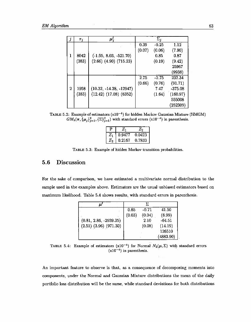
EM Algorithm
J 1íj µ~ Ei 0.39 -0.25 1.12
(0.07) (0.06) (7.90) 1 8042 (-1.95, 8.03, -521.70) 0.85 0.87
(383) (2.66) ( 4.90) (715.23) (0.19) (9.42) 25967 (9938)
2.75 -2.75 232.34 (0.66) (0.76) (91.71)
2 1958 (10.32, -14.38, -12947) 7.47 -375.08 (383) (12.42) (17.08) (6352) (1.64) (160.97)
555008 (252309)
TABLE 5.2: Example of estimators {xl0-4) for hidden Markov Gaussian Mixture (HMGM) GM3(1r, {µilJ=l• {E}J=1) with standard errors (x10-· 4
) in parenthesis.
]p> Z1 Z2 Z1 0.9477 0.0423 Z2 0.2167 0.7833
TABLE 5.3: Example of hidden Markov transition probabilities.
5.6 Discussion
63
For the sake of comparison, we have estimated a multivariate normal distribution to the
sample used in the examples above. Estimators are the usual unbiased estimators based on
maximum likelihood. Table 5.4 shows results, with standard errors in parenthesis.
µt E 0.85 -0.71 41.50
(0.03) (0.04) (8.99) (0.81, 2.86, -2939.35) 2.10 -64.51 (2.51) (3.96) (971.30) (0.08) (14.19)
126510 (4883.90)
TABLE 5.4: Example of estimators {xl0-4) for Normal N3(µ, E) with standard errors {xl0- 4 ) in parenthesis.
An important feature to observe is that, as a consequence of decomposing moments into
components, under the Normal and Gaussian Mixture distributions the mean of the daily
portfolio loss distribution will be the same, while standard deviations for both distributions
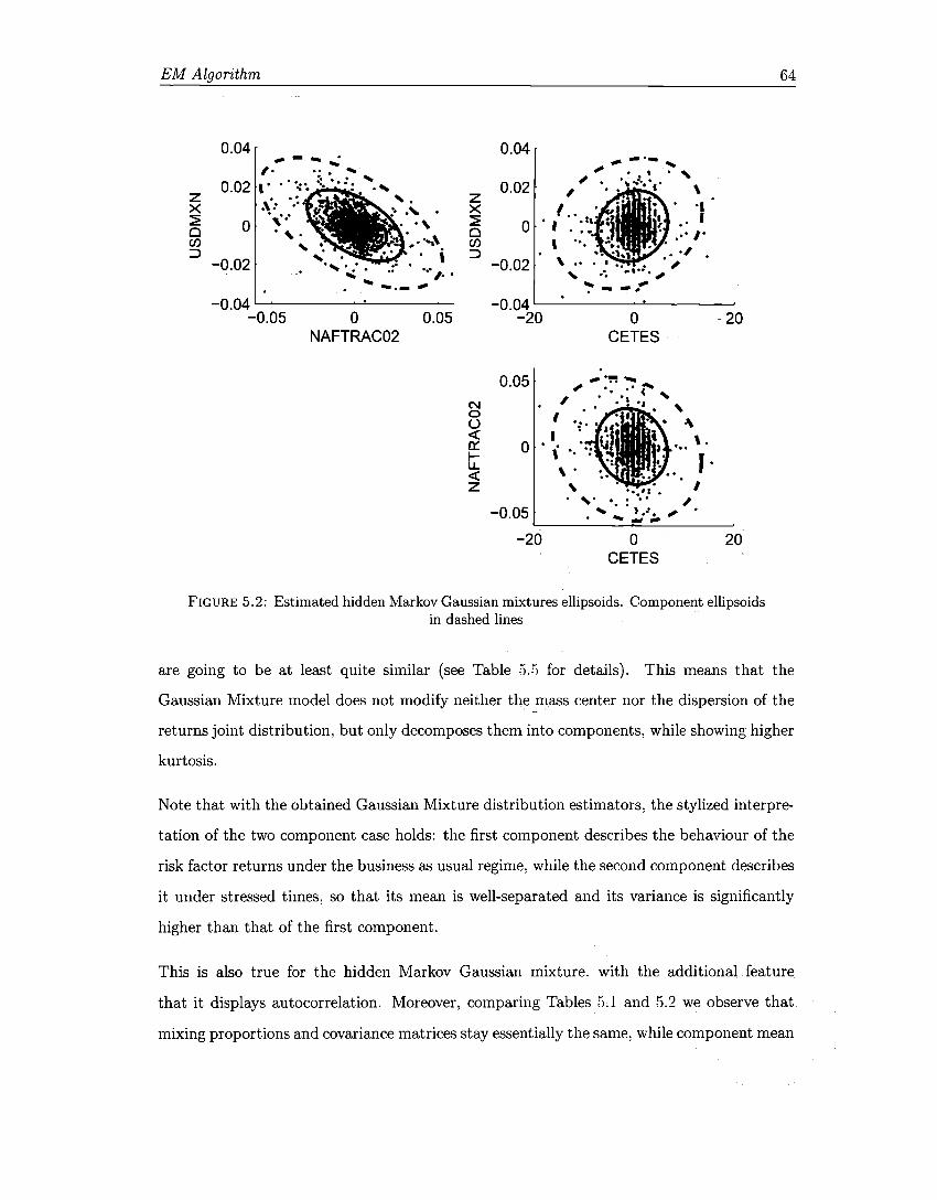
EM A lgorithm
z >< ~ Cl (/)
::>
0.04
0.02
o
-0.02
-- .... ,. ·: :- ... '. ····· •: •.:.' ... ~ .. , . . . -
.\: .. ; ·,··· . ' -~~-... ·_ ..... , ' . . . . ,· ·,. . .: . .... . .. . .. .... , .. --- --0.04 ~---~--~-
-0.05 O 0.05 NAFTRAC02
z X ~ Cl (/) ::J
N o ü <( o:: 1--u. <( z
0.04
0.02
o
-0.02.
' ~--0.04
. -20 o 20
CETES
1
0.05
o
' ~- I . ,. ·. : .. , -0.05 ... ) ., . , . .... ~ -
-20 o 20 CETES
FIGURE 5.2: Estimated hidden Markov Gaussian mixtures ellipsoids. Component ellipsoids in dashed lines
64
are going to be at least quite similar (see Table 5.!"í for details). This means that the
Gaussian Mixture model <loes not modify neither the mass center nor the dispersion of the
returns joint distribution, but only decomposes them into components, while showing higher
kurtosis.
Note that with the obtained Gaussian Mixture distribution estimators, the stylized interpre
tation of the two component case holds: the first component describes the behaviour of the
risk factor returns under the business as usual regime, while the second component describes
it under stressed times, so that its mean is well-separated and its variance is significantly
higher than that of the first component.
This is also true for the hidden Markov Gaussian mixture. with the additional feature
that it displays autocorrelation. Moreover, comparing Tables 5.1 and 5.2 we observe that
mixing proportions and covariance matrices stay essentially the same, while component mean
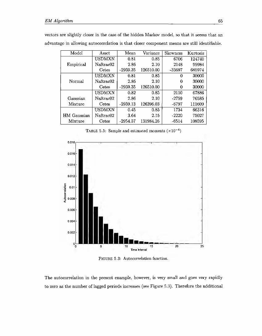
EM Algorithm 65
vectors are slightly closer in the case of the hidden Markov model, so that it seems that an
advantage in allowing autocorrelation is that closer component means are still identifiable.
Model Asset Mean Variance Skewness Kurtosis USDMXN 0.81 0.85 6706 124740
Empirical Naftrac02 2.86 2.10 2148 99984 Cetes -2939.35 126510.00 -33697 685974
USDMXN 0.81 0.85 o 30000 Normal Naftrac02 2.86 2.10 o 30000
Cetes -2939.35 126510.00 o 30000 USDMXN 0.82 0.85 2110 67886
Gaussian Naftrac02 2.86 2.10 -2759 76585 Mixture Cetes -2939.13 126396.03 -6797 111609
USDMXN 0.45 0.85 1734 66316 HM Gaussian Naftrac02 3.64 2.15 -2220 75027
Mixture Cetes -2954.57 131984.26 -6514 108595
TABLE 5.5: Sample and estimated moments (xl0- 4)
0.018~----------------~----------~
0.016
0.014
0.012
e: ,8 0.01 IU
~ 8 ~ 0.008 <(
0.006
0.004
0.002
o o 5 10 15 20 25
Time interval
FIGURE 5.3: Autocorrelation function.
The autocorrelation in the present example, however, is very small and goes very rapidly
to zero as the number of lagged periods increases (see Figure 5.3). Therefore the additional
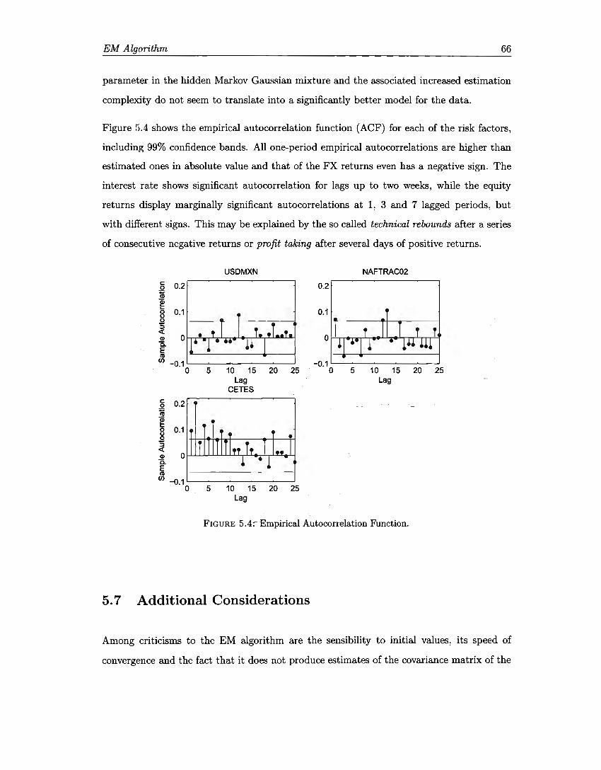
EM Algorithm 66
parameter in the hidden Markov Gaussian mixture and the associated increased estimation
complexity do not seem to translate into a significantly better model far the data.
Figure 5.4 shows the empirical autocorrelation function (ACF) far each of the risk factors,
including 99% confidence bands. All one-period empirical autocorrelations are higher than
estimated ones in absolute value and that of the FX returns even has a negative sign. The
interest rate shows significant autocorrelation far lags up to two weeks, while the equity
returns display marginally significant autocorrelations at 1, 3 and 7 lagged periods, but
with different signs. This may be explained by the so called technical rebounds after a series
of consecutive negative returns or profit taking after several days of positive returns.
USDMXN NAFTRAC02 e: 0.2 0.2 o i ~ 0.1f 1 0.1 o . ~ :, <( Q) Q 1 1 r•e I I i I .IIW 1 • 1 t 1 • i T I ee 1 • 1 o 0. E (11
(/) -0.1 -0.1 o 5 10 15 20 25 o 5 10 15 20 25
Lag Lag CETES
e: 0.2 o ~ ~
0.1 o E :, <( Q) o 0. E (11
(/) -0.1 o 5 10 15 20 25
Lag
FIGURE 5.4: Empirical Autocorrelation Function.
5. 7 Additional Considerations
Among criticisms to the EM algorithm are the sensibility to initial values, its speed of
convergence and the fact that it does not produce estimates of the covariance matrix of the
EM Algorithm 67
MLEs. Subsequent developments have addressed these shortcomings. Here we only review
a few topics, for further details on the EM algorithm see McLachlan and Krishnan [55] and
about its application to Gaussian mixtures, see McLachlan and Peel [53].
5.7.1 Starting Values
As explained in Algorithms 5.1 and 5.3 the EM algorithm is started from sorne initial value
for the parameters. Seidel, Mosler and Alker [73] have demonstrated how different starting
values and stopping criteria lead to quite different estimates in the context of exponential
components.
As convergence with the EM algorithm may be slow, the situation will be exacerbated by a
poor choice of the starting values. Indeed, in sorne cases where the likelihood is unbounded
(like normal components in mixture distributions) the sequence of estimates generated by
the algorithm may diverge if it is started too close to the boundary.
For example, an ad hoc way of initially partitioning the data might be obtained through
the use of sorne clustering algorithm, such as k-means or a hierarchical procedure if the
sample size is not too large. From there, initial estimates of the component parameters are
obtained.
Another way of specifying an initial partition of the data is to randomly divide the data
into g groups and getting from there component-specific initial estimates. With random
starts (actually, a number of them), the effect of the central limit theorem tends to have
the component parameters initially being similar at least in large samples. lt should be
noted that in the fitting of a mixture of d-dimensional normal components with unrestricted
covariance matrices, there needs to be at least d+ 1 observations assigned to each component
to ensure nonsingular estimates of the component covariance matrices.
An alternative method of specifying a random start in the context of g normal components
is to randomly generate components means from a normal distribution with mean equal to
the sample mean and covariance equal to the sample covariance matrix. The component
EM Algorithm 68
covariance matrices starting values can be specified as the sample covariance matrix and
the initial proportions can be randomly sampled from a uniform distribution and properly
rescaled to sum up to one. With this method there is more variation in between the initial
values for the mean vectors than with a random partition of the data into groups an it is
computationally less demanding.
This is the approach that we have followed to select starting values, the Matlab function
written with this purpose is in the Appendix. The only difficulty that we have found is
that, from time to time, one of the proportions estimates goes to zero. In the case of g = 2
components, this means recovering the normal distribution.
5. 7.2 N umerical Instabilities
As explained in Leroux and Puterman [46), the forward-backward algorithm of section 5.5
for the calculation of a;t and b;t is numerically unstable in ma.ny situations. This is because
a;t converges rapidly to zero or diverges to infinity as t increases, thus making it impossible
to calculate and store long sequences. Various methods have been proposed for avoiding
this problem. The same authors, for instance, suggest re-scaling a;t and bjt, reconstruct
ing afterward the original values to compute Tjt and Tijt; see also Turner, Cameron, and
Thomson [82].
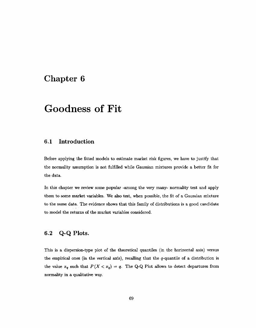
Chapter 6
Goodness of Fit
6.1 Introduction
Before applying the fitted models to estimate market risk figures, we have to justify that
the normality assumption is not fulfilled while Gaussian mixtures provide a better fit for
the data.
In this chapter we review sorne popular -among the very many- normality test and apply
them to sorne market variables. We also test, when possible, the fit of a Gaussian mixture
to the same data. The evidence shows that this family of distributions is a good candidate
to model the returns of the market variables considered.
6.2 Q-Q Plots.
This is a dispersion-type plot of the theoretical quantiles (in the horizontal axis) versus
the empirical ones (in the vertical axis), recalling that the q-quantile of a distribution is
the value Xq such that P (X< xq) = q. The Q-Q Plot allows to detect departures from
normality in a qualitative way.
69
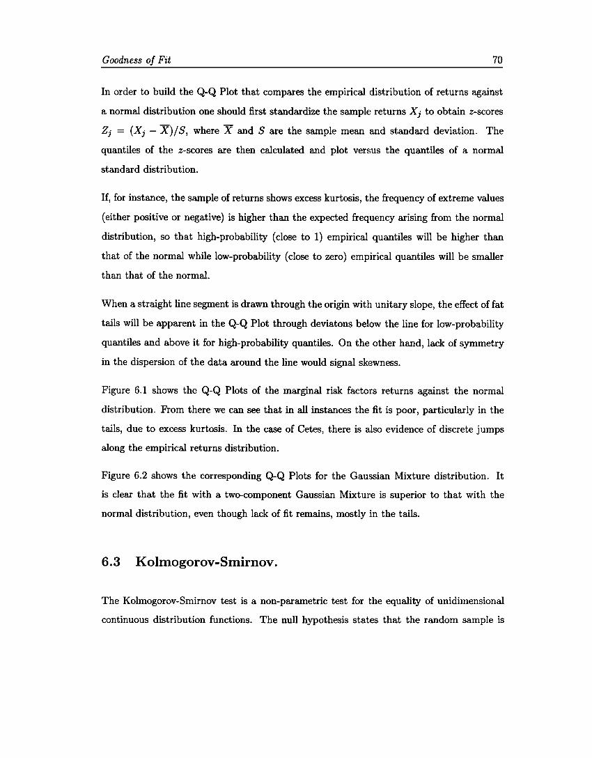
Goodness of Fit 70
In arder to build the Q-Q Plot that compares the empirical distribution of returns against
a normal distribution one should first standardize the sample returns Xi to obtain z-scores
Zi = (Xj - X}/S, where X and S are the sample mean and standard deviation. The
quantiles of the z-scores are then calculated and plot versus the quantiles of a normal
standard distribution.
If, for instance, the sample of returns shows excess kurtosis, the frequency of extreme values
(either positive or negative) is higher than the expected frequency arising from the normal
distribution, so that high-probability ( close to 1) empirical quantiles will be higher than
that of the normal while low-probability (close to zero) empirical quantiles will be smaller
than that of the normal.
When a straight line segment is drawn through the origin with unitary slope, the effect of fat
tails will be apparent in the Q-Q Plot through deviatons below the line for low-probability
quantiles and above it for high-probability quantiles. On the other hand, lack of symmetry
in the dispersion of the data around the line would signal skewness.
Figure 6.1 shows the Q-Q Plots of the marginal risk factors returns against the normal
distribution. From there we can see that in ali instances the fit is poor, particularly in the
tails, dueto excess kurtosis. In the case of Cetes, there is also evidence of discrete jumps
along the empirical returns distribution.
Figure 6.2 shows the corresponding Q-Q Plots for the Gaussian Mixture distribution. lt
is clear that the fit with a two-component Gaussian Mixture is superior to that with the
normal distribution, even though lack of fit remains, mostly in the tails.
6.3 Kolmogorov-Smirnov.
The Kolmogorov-Smirnov test is a non-parametric test for the equality of unidimensional
continuous distribution functions. The null hypothesis states that the random sample is
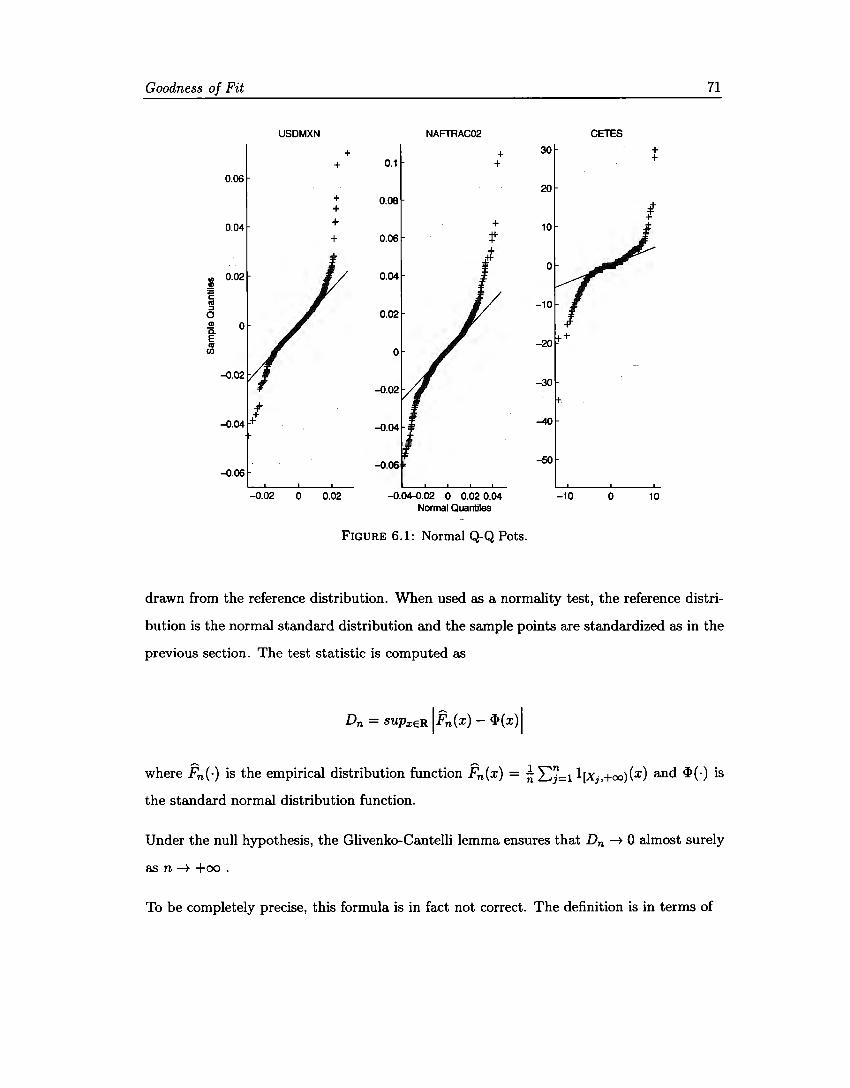
Goodness of Fit 71
USDMXN NAFTRAC02 CETES
+ + 30 + +
+ 0.1 + 0.06
20 + 0.08 + t + +
0.04 + 10 + 0.06 f
,;t o
UI 0.02 0.04 .!!! E "' -10 ::, o 0.02 a, o a. E -20 "' C/) o
-0.02
-0.02 -30
t -0.04 + -40
-0.04
-0.06 -50 -0.06
-0.02 o 0.02 -0.04-0.02 o 0.02 0.04 -10 o 10 Normal Quantiles
FIGURE 6.1: Normal Q-Q Pots.
drawn from the reference distribution. When used as a normality test, the reference distri
bution is the normal standard distribution and the sample points are standardized as in the
previous section. The test statistic is computed as
where Fn(·) is the empirical distribution function Fn(x) = ¼ "¿,j=l l[x;,+oo)(x) and <I>(-) is
the standard normal distribution function.
Under the null hypothesis, the Glivenko-Cantelli lemma ensures that Dn ~ O almost surely
as n ~ +oo.
To be completely precise, this formula is in fact not correct. The definition is in terms of
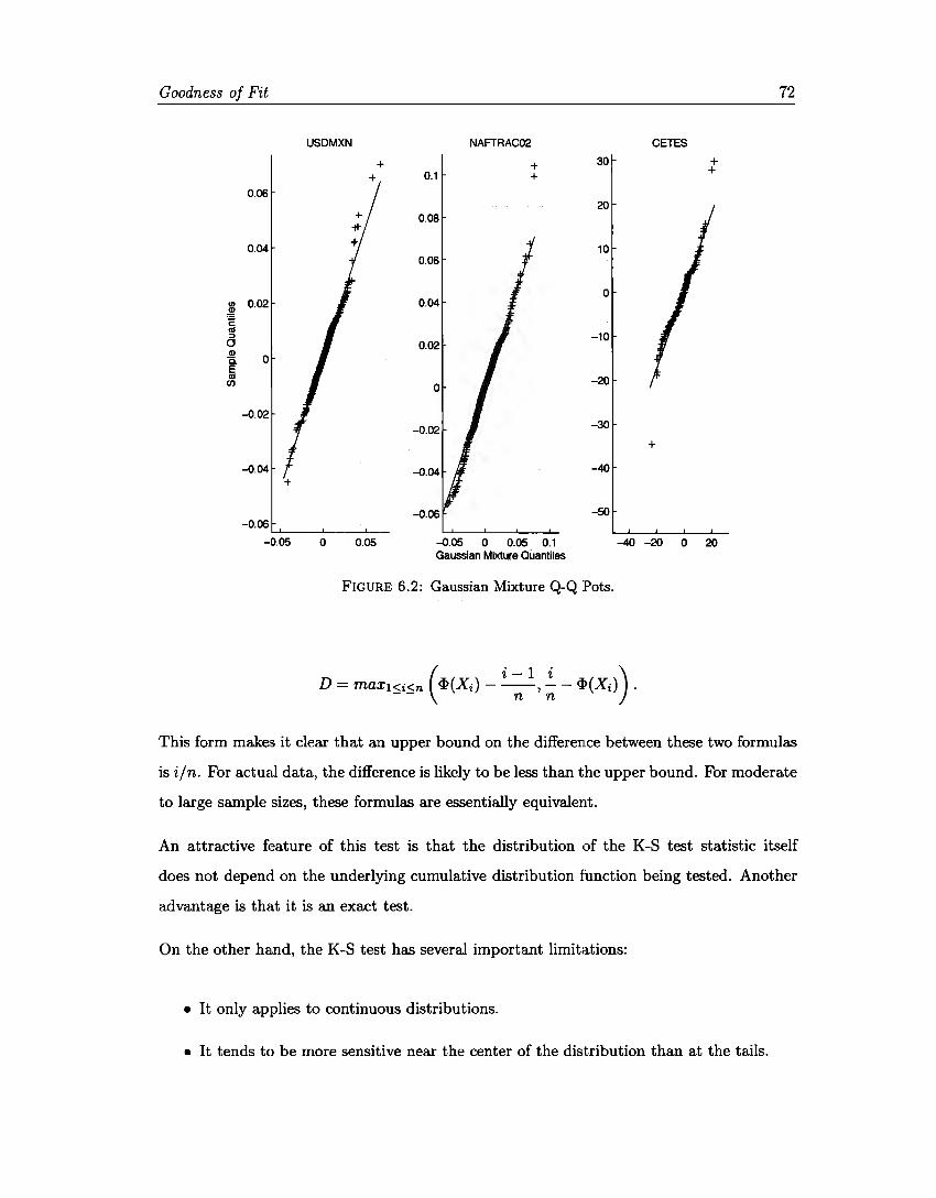
Goodness of Fit 72
USDMXN NAFTRAC02 CETES
+ + 30 + + + 0.1 +
0.06 20
0.08
0.04 10 0.06
o fll 0.02 0.04 ~ E <11
-10 :::, o 0.02 CD o Q. E <11 -20 en o
-0.02 -0.02 -30
+
-0.04 -0.04 -40 +
-0.06 -50 -0.06
-0.05 o 0.05 -0.05 o 0.05 0.1 -40 -20 o 20 Gaussian Mixture Quantiles
FIGURE 6.2: Gaussian Mixture Q-Q Pots.
D = max1<i<n <l>(Xi) - --, - - <l>(Xi) . ( i-1 i )
- - n n
This form makes it clear that an upper bound on the difference between these two formulas
is i/n. For actual data, the difference is likely to be less than the upper bound. For moderate
to large sample sizes, these formulas are essentially equivalent.
An attractive feature of this test is that the distribution of the K-S test statistic itself
<loes not depend on the underlying cumulative distribution fi.rnction being tested. Another
advantage is that it is an exact test.
On the other hand, the K-S test has several important limitations:
• It only applies to continuous distributions.
• It tends to be more sensitive near the center of the distribution than at the tails.

Goodness of Fit 73
• The distribution must be fully specified.
The last one is perhaps the most serious limitation. That is, if location, scale, and shape
parameters are estimated from the data, the critica! region of the K-S test is no longer
valid. This overlies the first advantage above as in practice the critica! values for have to be
determined by simulation.
Therefore, in the case of unknown parameters, Lilliefors [47] used the same test statistic
as before and corrected the rejection region to account for uncertainty in the estimated
parameters, giving rise to the Lilliefors test. Even with this correction the test is not as
powerful as the Anderson-Darling test (see Stephens [76]).
In fact, several goodness-of-fit tests, such as the Cramér von Mises test and the Anderson
Darling test, are refinements of the K-S test, in the sense that they are more powerful than
the K-S test.
6.4 Anderson-Darling.
This test is designed to assess whether a sample of data carne from a population with a
specific distribution Fo(·). The null hypothesis Ho : F(t) =: Fo(t), t E IR. is rejected if the
empirical distribution function Fn(t) is different from Fo(t) as measured by
l+oo
WJ = n _00
[Fn(t) - Fo(t)] 2 1/J(F0 (t))dF0 (t).
If 1/J (u) = 1 then the statistic WJ is the Cramér von Mises test statistic, denoted by n w2•
Consider now the empirical distribution function
1 n
Fn(t) = n L l{x;9}• j=l
where nis the sample size and lA is the indicator function of the set A. For a given Fo(t) it
can be seen as a weighted sum of independent Bernoulli random variables with probability
Goodness of Fit 74
F0 (t). Therefare, nFn(t) is a binomial random variable with parameters n and Fo(t). Its
expected value is nFo(t) and its variance is nF0(t)[l-Fo(t)]. Then, under the null hypothesis
...fñ, Fn(t) - Fo(t)
JFo(t)[l - Fo(t)]
has zero mean and unitary variance. Anderson and Darling [3] suggested the weight function
1 1/J(u) = Fo(t)[l - Fo(t)]' (6.1)
which places more emphasis on the deviation at the tails of the distribution and in this sense
is a modification of the KS test. Their choice of weight function leads to the test statistic
A~= n f+oo [Fn(t) - Fo(t)]2 dFo(t). }_00 Fo(t) [1 - Fo(t)]
They also showed that it can be written as
2 ~ 2i - 1 [ ( )] An = -n - L.,,,-- logFo(X(i)) + log 1 - Fo(X(n+l-i)) n
i=l
where X(i) are the ordered statistics.
(6.2)
The test is a one--sided test and the hypothesis that the distribution is of a specific farm
is rejected if the test statistic A~ is greater than the critica] value. Anderson and Darling
faund the limiting distribution of A~ far the weight function {6.1). The 5% critica! value
of the limiting distribution is 2.492 and the 1 % value is 3.880. The mean of this limiting
distribution is 1 and the variance is 2(71"2 - 9)/3 ~ 0.57974.
The Anderson-Darling test makes use of the specific distribution in calculating critica! values.
This has the advantage of allowing a more sensitive test ancl the disadvantage that critica!
values must be calculated far each distribution. Stephens [76] analysed the behaviour of
Goodness of Fit 75
the test statistic when the parameters are replaced by estimators and computed adjusted
p-values.
6.5 Jarque-Bera.
The Jarque-Bera [39) is a test specifically designed to test for normality when parameters
are unknown. It is defined in terms of the estimators of skewness and excess kurtosis, given
a sample of size n. The test statistic is
JB=n ~+~ (~2 ~2) 6 24 '
where r = E[(X - µ)3]/o-3 is the skewness and K- = E[(X - µ) 4]/o-4 - 3 is the excess kurtosis.
The J B test statistic follows asymptotically a chi-square distribution with 2 degrees of
freedom under the null hypothesis that the random sample comes from a normal distribution
with meanµ and standard deviation a. In such case, r = K- = O as the normal distribution
is symmetric and the benchmark measure for kurtosis.
Due to the square exponents in the test statistic J B, high values of it imply departures from
normality (either from lack of symmetry or excess kurtosis), therefore the Jarque-Bera is a
one-tail test and the rejection region correspond to values that exceed a threshold depending
on the confidence level of the test.
Under the null hypothesis, standard errors of the estimators of r and K- are approximately
rn )112 and ( ~) 112
' where n is the sample size. In other words, the standard error of the
estimator of kurtosis doubles that of the estimator of skewness.
Table 6.1 displays test statistics and p-values for Kolmogorov-Smirnov (KS), Anderson
Darling (AD) and Jarque-Bera (JB) normality tests for the returns of three risk factors. JB
and KS tests are to be rejected even at very high confidence levels, while AD test is rejected
at confidence levels up to 99%, indicating that marginal return distributions are certainly
not normal. The joint distribution can not be normal either.
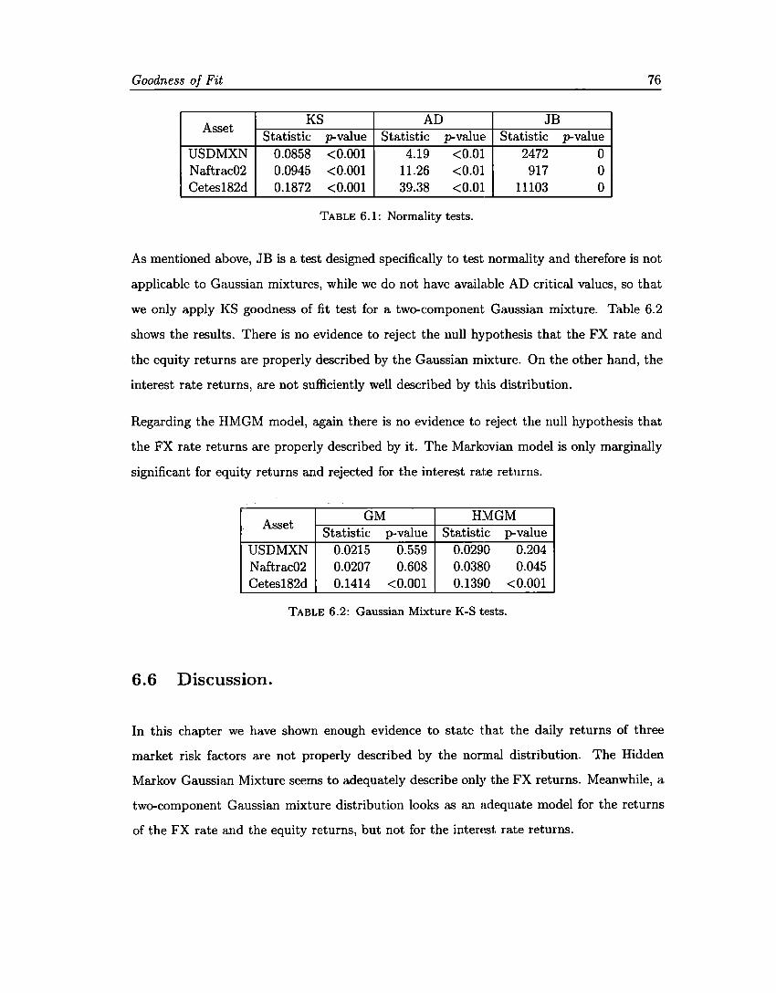
Goodness of Fit 76
Asset KS AD JB
Statistic p-value Statistic p-value Statistic p-value USDMXN 0.0858 <0.001 4.19 <0.01 2472 o Naftrac02 0.0945 <0.001 11.26 <0.01 917 o Cetes182d 0.1872 <0.001 39.38 <0.01 11103 o
TABLE 6.1: Normality tests.
As mentioned above, JB is a test designed specifically to test normality and therefore is not
applicable to Gaussian mixtures, while we do not have available AD critica} values, so that
we only apply KS goodness of fit test for a two-component Gaussian mixture. Table 6.2
shows the results. There is no evidence to reject the null hypothesis that the FX rate and
the equity returns are properly described by the Gaussian mixture. On the other hand, the
interest rate returns, are not sufficiently well described by this distribution.
Regarding the HMGM model, again there is no evidence to reject the null hypothesis that
the FX rate returns are properly described by it. The Markovian model is only marginally
significant for equity returns and rejected for the interest rate returns.
Asset GM HMGM
Statistic p-value Statistic p-value USDMXN 0.0215 0.559 0.0290 0.204 Naftrac02 0.0207 0.608 0.0380 0.045 Cetes182d 0.1414 <0.001 0.1390 <0.001
TABLE 6.2: Gaussian Mixture K-S tests.
6.6 Discussion.
In this chapter we have shown enough evidence to state that the daily returns of three
market risk factors are not properly described by the normal distribution. The Hidden
Markov Gaussian Mixture seems to adequately describe only the FX returns. Meanwhile, a
two-component Gaussian mixture distribution looks as an adequate model for the returns
of the FX rate and the equity returns, but not for the interest rate returns.
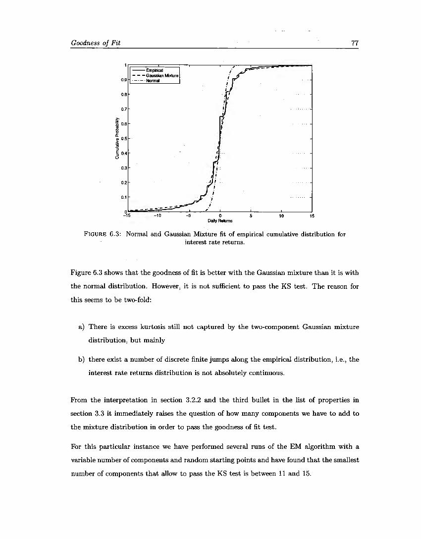
Goodness of Fit
--Empirical - - - Gaussian Mixture
0.9 · - · - · Normal
0.8
0.7
~ 0.6 :a
"' IJ e o. ., 0.5 > 1i "5 E 0.4 ::, u
0.3
0.2
0.1
-- -·-o -15 -10 -5
,. I
1 ,. 1
• I 1
1
,, 1 J
o Daily Retums
---
5 10 15
FIGURE 6.3: Normal and Gaussian Mixture fit of empirical cumulative distribution for interest rate returns.
77
Figure 6.3 shows that the goodness of fit is better with the Gaussian mixture than it is with
the normal distribution. However, it is not sufficient to pass the KS test. The reason for
this seems to be two-fold:
a) There is excess kurtosis still not captured by the two-component Gaussian mixture
distribution, but mainly
b) there exist a number of discrete finite jumps along the empirical distribution, i.e., the
interest rate returns distribution is not absolutely continuous.
From the interpretation in section 3.2.2 and the third bullet in the list of properties in
section 3.3 it immediately raises the question of how many components we have to add to
the mixture distribution in order to pass the goodness of fit test.
For this particular instance we have performed several runs of the EM algorithm with a
variable number of components and random starting points and have found that the smallest
number of components that allow to pass the KS test is between 11 and 15.
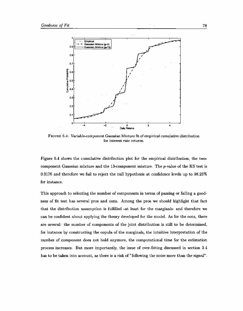
Goodness of Fit
.. · ... · Empirical · - · - · Gaussian Mixture (g=2)
0.9 --Gaussian Mixture (g=13)
o.e
0.7
2:-'B 0.6 i e Q. ~ 0.5 ¡¡ 'S 5 0.4 o
0.3
0.2
0.1
I
I
¡
I
I
o~-~----~----~----~---~~-~ -4 -2 o 2 4
Daily Aeturns
FIGURE 6.4: Variable-component Gaussian Mixture fit of empirical cumulative distribution for interest rate returns.
78
Figure 6.4 shows the cumulative distribution plot for the empirical distribution, the two
component Gaussian mixture and the 13-component mixture. The p-value of the KS test is
0.0176 and therefore we fail to reject the null hypothesis at confidence levels up to 98.25%
for instance.
This approach to selecting the number of components in terrns of passing or failing a good
ness of fit test has several pros and cons. Among the pros we should highlight that f act
that the distribution assumption is fulfilled -at least for the marginals- and therefore we
can be confident about applying the theory developed for the model. As for the cons, there
are several: the number of components of the joint distribution is still to be determined,
for instance by constructing the copula of the marginals, the intuitive interpretation of the
number of component <loes not hold anymore, the computational time for the estimation
process increases. But more importantly, the issue of over-fitting discussed in section 3.4
has to be taken into account, as there is a risk of "following the noise more than the signal".
Goodness of Fit 79
6. 7 Goodness of fit for unrestricted Gaussian Mixtures.
From n independent realizations of a random variable (rv), X say {x1, x2 , ... , xn}, with
density function J(-) with support in IR, we want to assess the distributional assumption
g ( ) 1 x-µ·
Ho: f(x) = "'Trj-</> 1 ,
~ a· a· j=l J J
where cp(z) = 1¡..¡,¡; exp(-z2 /2) is the standard normal density function and °I:]=l 'lfj = 1,
with O < 'lfj < l. That is, we want to verify if the rv X follows a g-component Gaussian
Mixture with arbitrary parameters (means, variances and mixing proportions).
We have explored above the strategy of adding components to the mixture until the KS
goodness of fit test fails to reject H 0 . However, we have also mentioned the limitations of
this test in section 6.:3 above, in particular, the fact that the assumed distribution should be
continuous and completely specified, as well as it feature of privileging the fit in the center
of the distribution (which is clear in Figure 6.4). Therefore we should exercise care when
using this approach.
Moreover, taking into account that selecting the number of components in a mixture distri
bution is still an open question we should explore the line of developing a specific goodness
of fit test for finite Gaussian Mixture distributions that avoids the difficulties of dealing with
the likelihood function and makes use of the semi-parametric features of the mixture models
to provide guidance on the optima! number of components to be included in the mixture.
Optimality in this case should be understood as a balance between parsimony and goodness
of fit.
Chapter 7
Market Risk using Gaussian
Mixtures
7.1 lntroduction
In this chapter we derive the -aggregated- Portfolio Loss Distribution following the lines
of McNeil, et. al. [57]. According to loss distribution literature, we assume that losses
are positive and profits are negative. We find the linear approximation of the loss function
through a loss operator that is approximately equal to it for small changes in the underlying
risk factors.
In section 7.3, we formally define the standard market risk measures to be calculated on
the loss distribution and obtain their estimators under four different models. In particular,
we contribute with a closed-form expression for the expected shortfall of a finite Gaussian
mixture distribution, including its derivation. A particular case of our expression is used by
Kamaruzzaman and Isa [41] to estimate VaR and ES for monthly and weekly returns of a
Malaysian stock index.
80
Market Risk using Gaussian Mixtures 81
Later we propase a multi-asset-type portfolio and estimate sensibilities to risk factors. We
then fit multivariate Normal and stationary and autocorrelated Gaussian Mixtures distribu
tions and estimate market risk measures (VaR and ES) under all models (three parametric
and one no parametric).
In order to select among models, we review backtesting procedures for each risk measure
and apply them to each asset and the portfolio. Another contribution comes in the form of a
procedure to raise early alerts in the case risk figures are likely not to pass a back-test. This
is based on the equivalence between hypothesis testing and confidence intervals, standard
errors obtained in section 3.6 and asymptotic theory of MLEs. We finish the chapter with
a brief discussion of the results.
7.2 Portfolio Loss Distribution
Given a portfolio of assets subject to market risk, consider the aggregated -profit and- loss
random variable for the time interval [t~, (t + 1)~]:
L¡ta,(t+1)aJ = Lt+1 = -(½+1 - ½) = -[f(t + 1, Zt + .Xt+1) - f(t, Zt)]
where
L¡t,t+r) is the loss over the time interval [t, t + r],
r is the investment horizon. We will assume that t is measured in days and that the
investment horizon is one day ( r = l), therefore
Lt+ 1 is the portfolio loss from day t to day t + 1,
Vi = J(t, Zt) is the portfolio market value at time t,
/ : JR+ x JRd -+ IR is a measurable function,
Zt E JRd is the d-dimensional vector of risk factors at time t,
Market Risk using Gaussian Mixtures 82
Xt = Zt - Zt-1 contains the risk factor returns from day t - 1 to day t.
According to the above definitions, losses are positive and profits are negative. As the value
of risk factors Zt is known at time t, the loss distribution is completely determined by the
distribution of risk factor returns in the following period. It is then possible to define the
loss operator lt : ]Rd -+ IR that maps risk factor returns into portfolio loss:
lt(x) = - [f (t + 1, Zt + x) - f(t, Zt)], x E ]Rd_ (7.1)
Observe that Lt+l = lt(Xt+1)- If the function f is differentiable, it is possible to write the
linear approximation ( delta in derivatives nemotecnia) of the loss operator lt in equation
(7.1) as
lf(x) = - [ft(t, Zt) + t fz,(t, Zt)Xjl = - ( Ct + w~x), J=l
(7.2)
where
Ct = ft(t, Zt) ~ O for small time increments, such as one day,
w~ = (f z, ( t, Zt)) :=l is the vector of risk factor sensitivities, and
fu(t, ·) = 8J(t, ·)/ou.
If the function f has non-vanishing second-order derivatives, the approximation (7.2) can
include them, producing a Delta-Gamma model. The loss operator (and random variable)
moments are, from equation (7.2):
Market Risk using Gaussian Mixtures
d
ELt+l ~ El¡'(X) = - L fz;(t, Zt}EXi = w~µ = µL j=l
~ ' 2 Var(Lt+1) ~ Var(lt (X)}= wtEWt = o-L,
with µ' = (EXj};=l and Ei,i = cov(Xi,Xj)-
83
(7.3}
In what follows we will assume that returns Xt come from a stationary process to ease
notation, that is, they are iid random vectors and so we can omit the t subscript. See
Chapter 3 in Meucci [59] for a thorough discussion on what he calls market invariants.
7.3 Market Risk Measures
Once we derive the portfolio loss distribution, the investor may choose between portfolios
preferring the one that is more advantageous in a global sense. Stochastic dominance is at
first glance an alternative but it has a few drawbacks, in particular, it is not a total order,
i.e., two portfolios might no necessarily be comparable (the concept of stochastic dominance
is treated in detail in Pennacchi [63] and also in Meucci [59]}. Therefore we need sorne
metrics to summarize the key properties of the risk that the portfolio is exposed to.
We should ask to the summarizing metrics sorne properties (see Arztner et al [4]}, such as
estimability -or law invariance-, consistency with stochastic dominance, constancy, homo
geneity, translation invariance, additivity, convexity, risk aversion.
Two broad classes of risk measures have become popular among academics and practitioners:
a) quantile-based risk measures for a given confidence level, better known as Value at
Risk. It has become a standard tool among financia! institutions after the Basel
Committee enforced its use to monitor the riskiness of their investments and
b) coherent risk measures, which are defined axiomatically in terms of their properties
Market Risk using Gaussian Mixtures 84
Market Risk mea.sures to be estimated are Value at Risk and Expected Shortfall, as defined
below, according to McNeil et. al. [57].
Definition 7.1. (VaRa,)- Let L be a -positive- loss random variable and FL : lR.-+ [O, 1] its
distribution function. We define Value at Risk at confidence level o E (O, 1) as
VaR°' := inf {u E lR.: FL(u) ~o}.
Definition 7.2. (ESa,)- Let L and FL : lR.-+ [O, 1] be as above. Suppose also that EJLJ < oo.
Expected Shortfall at confidence level o E (O, 1) is defined as
1 11 ES°' := -- VaRu,du. 1-o °'
It is clear that VaR°' is just the o-quantile of the loss distribution: VaR°' = qa,(FL) = F¡;1(o) and that ESa, is the average of all quantiles above confidence level o, as long as the
loss distribution is continuous.
Acerbi and Tasche [1] provide a generalized ES definition that includes the case of non
continuous loss distributions (such as the empirical distribution), introducing a term to
correct the bias of V aR°' as an estimator of the o-quantile:
Definition 7.3. (GESa)- Let L and FL be as in Definition 7.2. Generalized Expected
Shortfall at confidence level o E (O, 1) is
GESa := l ~ 0 [¡1
VaRu,du + qª (1- o - P (L ~ VaRa))].
For continuous distributions Definitions 7.2 and 7.3 coincide and the following proposition
provides a useful tool for calculations. The proof is in the Appendix A.2.
Market Risk using Gaussian Mixtures 85
Proposition 7.4. If L is a loss random variable with continuous distribution function FL
and EILI < oo, then
ES0 = E [LIL ~ VaR0 ]. (7.4)
If the distribution of L is a location and scale distribution, VaR calculation depends only
on the moments described in equations (7.3):
(7.5)
where q0 is the quantile in Definition 7.1 for a distribution function FL with location pa
rameter zero and scale parameter one.
Property 3.3 guaranties that under the Delta-Normal model, the random variable L follows
a univariate Normal distribution and in this case equation (7.5) provides our VaR estimator.
For the non-parametric model (HS) the distribution of L is the empirical distribution and
it suffices to take the appropriate order statistic to obtain
-VaR0 = L(lnaJ), (7.6)
where L(j) is the jth order statistic, n is the sample size, and L;z: J is the biggest integer that
is less than or equal to x. Finally, for the Delta-GM model, Property 3.4 ensures that the
distribution of L is a univariate finite Gaussian Mixture and it is necessary to solve for q0
the following equality:
(7.7)
With respect to ES, for the HS model it is built using the empirical distribution and Def
inition 7.2 or 7.3 together with expression (7.6). The Appendix contains the proof of the
expression for the Delta-Normal model while for the finite Gaussian Mixture model the
proposition below states the closed-form expression for the ES.
Market Risk using Gaussian Mixtures 86
Proposition 7.5. lf L is a loss mndom variable with densit:,¡ function as in Definition 3.2
and distribution function FL , then for a E [O, 1]
(7.8)
Proof. Let L "" M N (1r, µ, u), recall that Qc,; = VaRo: is the solution of equation (7.7):
FL (qc,;; 1r, µ, u) - a = O. From Definition 7.1, equation (7.4) and the distribution of L, we
have
The integral within the sum is the same as equation (A.2) in Appendix A, with the only
difference that the lower limit of the integral depends on the specific component. Making
the change of variable u= UjZ + µj and defining Zj,o: = (qc,; - µj)/ui we obtain an analogous
result to (A.3):
D
Note that Zj,o: depends on a through qc,; and on the component through parameters µj and
Uj, but it is not the a-quantile of the j-th component distribution, that is to say, it is not the
Market Risk using Gaussian Mixtures 87
case that <l>(zj,o:) = o:. In other words, µj +uj</>(zj,o:)/<1>(-zj,o:) is not the ES0 corresponding
to the j-th component.
It is possible, however, to write the finite Gaussian Mixture Expected Shortfall as the
weighted summation of the component-specific Expected Shortfalls. To see this, let Lj "'
N (µj, uJ), then, according to section A.3 of the Appendix:
= </> (<1>-l(o:))
µ. + (J'. ---'-----'-] J 1-o:
:. ES0 (L)
where
g
¿>.iES0 (Lj) j=l
).. . _ 1r. <1>(-zj,o:) µj + Uj</>(zj,o:)/<1>(-zj,o:) 3 - 3 l - o: µj + <J'j</> (<1>- 1(0:)) /(1 - o:).
In summary, the expressions for ES under the three models considered are as follows:
----HS ESo.
Delta-Normal ES0
l n
= n- Lno:J L L(j) i=Lno:J+I
= µ + l ~a</> (<1>-I(o:))
1 ~ [ </>(zj,o:) ] Delta-GM ES0 = -1
- L; 7rj<l>(-zj,o:) µj + <J'j <1>( ) - O: j=l -Zj,o:
7.4 Backtesting
(7.9)
Once risk figures are systematically estimated over time, the performance of the estimation
model can be monitored. This process of monitoring is known as backtesting and can also
be used to compare performance among different models, as suggested by Campbell [15].
Let us assume that for each time t we have one-period o:-level estimations for VaR and ES, - ----denoted VaRo:,t and ESo:,t, respectively. We can then define excess indicator and excess
loss random variables
Market Risk using Gaussian Mixtures 88
la(Lt+1) := 1 (v-R ) (Lt+I) and a o:,t,+oo
Ma,t+1(Lt+1) := ( Lt+l - ESa,t) la(Lt+1)- (7.10)
where lA(u) is the indicator function of the set A. The process {la(Lt)}tEN is a process of
iid Bernoulli random variables with success probability 1 - o. After estimating VaR figures
for times t = l, ... , n, we can expect that
n
I::Ia(Lt),..., Bin (n, 1 - o). t=l
Kupiec [44] constructs a test for
Ho : p = Po vs HA : p #- Po (7.11)
based on the likelihood ratio as test statistic. Asymptotically, this statistic follows a chi
square distribution with one degree of freedom, but for any given sample size exact rejection
regions can be calculated for the binomial distribution, as shown in Casella and Berger
[17] based on work by Casella [16]. We have written a Matlab function that implements
the exact test at a confidence level equal to that of the corresponding VaR estimation and
returns a non-rejection interval.
Turning now to ES, we should expect that excess losses behave like realizations of iid vari
ables from a distribution with mean zero andan atom of probability mass of size o at zero.
Testing the latter property is equivalent to backtesting VaR, so we will concentrate on a
procedure to test the former: zero-mean behaviour.
Recall first the one sample test under normal population for Ho : µ = µo. This can be
conducted using the test statistic z = vn(P, - µo)/a, which follows a normal distribution if
a is known or a Student t distribution if it is estimated.
Market Risk using Gaussian Mixtures 89
Efron and Tibshirani [25] propose a non-parametric bootstrap hypothesis test based on the
empirical distribution of the above test statistic under the null hypothesis, which in our case
is, from (7.10):
(7.12)
We will use the non-parametric bootstrap test for HS and a parametric bootstrap version
for the Delta-Normal and Delta-GM models.
The bootstrap test is conducted as follows: draw N samples of size n with replacement from
{ iña,t(lt) }~1 , as defined in (7.10), or from the fitted parametric distribution and for each
bootstrap sample, say m1, ... , mn, compute the statistic
iñ t(m)= a/.Jñ,' (7.13)
where a is the standard deviation of the bootstrap sample. The Achieved Significance Level
(ASL) for the alternative hypothesis HA : µ > O is estimated as
ASLboot = # {t (m) > tobs} /N, (7.14)
where tobs = t(ma) is the value of the statistic (7.13) observed in the original sample. We
test against a one-sided alternative based on the evidence of lack of symmetry of fiia (see
Figure 7.4), but can also test against a two-sided alternative.
As noted by Efron and Tibshirani, the estimate ASLboot has no interpretation as an exact
probability, but like all bootstrap estimates is only guaranteed to be accurate as the sample
size goes to infinity.
Market Risk using Gaussian Mixtures 90
7.5 Early Alerts
A clear limitation of the backtesting procedures reviewed in the previous section is that they
rely on asymptotic distributions, which translates into the necessity of a big sample size of
risk estimation and next-period loss figures befare a decision can be made.
In practice, if we use faur years of daily data to estimate risk measures and we backtest our
figures using at least ayear of daily risk calculations, then we have to wait at least 1250 days
befare we can decide whether the risk model is adequate. Or looking at it optimistically, at
least a year ( assuming we had available 1000 daily data far the first risk estimation).
Another shortcoming of backtesting is that there exist non-observable portions of the rejec
tion region of the null hypothesis. In particular, let us try to backtest VaR 99% based on a
year of daily risk estimations and next-day loss data, a samp]e of around 250 data points.
The non-rejection region of the test reviewed in the section above far this situation is [O, 6],
i.e., we regard the model to underestimate risk if there are more than 6 VaR excesses in any
given 12-month period. However, we are not able to detect if the model is over-estimating
risk as it is impossible to observe a negative number of excesses. This is true whenever risk
is estimated at a high confidence level.
In arder to overcome this limitations, we can profit from having calculated standard errors far
the Maximum Likelihood Estimators and from the parsimony of the expressions to calculate
VaR and ES far Gaussian Mixtures.
Let h( 0) be the risk measure (VaR or ES) as a function of the portfalio loss distribution
parameters. In the case of the Gaussian Mixture assumption, the portfalio loss distribution
is given by Property 3.4 and h(0) is given by q0 = Q(o; 0) = F¡: 1(o; 0) far VaR (equation
(7.7)) and Proposition 7.5 far ES. In either case, h(0) is a continuous function of its vector
parameter 0 = ( 0, {µj }]= 1, {o}}]= 1) and it is also differentiable. Let 0 !11LE be the MLE of
0.
Market Risk using Gaussian Mixtures 91
Therefore, by the invariance property of the MLE (see, for instance Casella and Berger [17])
h(8MLE) is also an MLE and, under the usual regularity conditions (that in sorne situations
may not apply to Gaussian Mixtures):
[h(OMLE) - h(8)] ~ N (o, Var(h(OMLE))) as n ---t +oo.
Even though this is also an asymptotic result, we make clear that n here refers to the sample
size used to estímate 8 (known as the time window in market risk management) as opposed
to the number of risk-estimation time periods in the usual backtesting procedures. So that
the result holds even from the very first time we estímate risk, as long as the time window
is big enough.
It suffices then to obtain or approximate Var(h(8MLE)) to construct a confidence interval
for h( 8). Sin ce h( ·) in general is not an easy function of 8 we first linearize it using a Taylor
series expansion of first order:
h(O) = h(8) + Vh(8)'(8 - 8) + Res,
where
8h(8) . (Vh(8))i = ----¡¡¡¡:-, J = 1, ... , m ~ 3g - l.
J
These partial derivatives can be computed explicitly or numerically, depending on the com
plexity of the function h(·). Therefore
h(O) - h(8) ~ Vh(8)'(8 - 8).
Now we approximate cov(O M LE) using I; 1 the inverse of the empírica} observed information
matrix, see section 3.6. In this way we obtain
Market Risk using Gaussian Mixtures 92
Var(h(8MLE)) ~ [Vh(0)'I; 1(0)Vh(0)] le=ijMLE --- ~ Vare(h(0MLE)). (7.15)
Then an asymptotic ó-level confidence interval for h(0) is given by
(7.16)
The following Proposition establishes the equivalence between backtesting and confidence
intervals for ES.
Proposition 7.6. Let h(·) be as in Proposition 7.5. Then testing the null hypothesis (7.12)
is equivalent to building the confidence interval (7.16).
Proof. From elementary statistics we know that there exist a correspondence between a
confidence interval and a test of hypothesis. The null hypothesis that is associated to the
confidence interval (7.16) is
Ho: h(0) = h(8). (7.17)
In section 7.4 we established the null hypothesis corresponding to VaR and ES backtesting
procedures. We clearly observe that (7.12) corresponds exactly to {7.17) as
E [Mo,t+I(Lt+i)] = E [ ( L- ESa) lL>VaRc.]
E [LI L > VaR0 ] - E [ESalL>VaRa]
- ESa - E (ESa)
:. E [Mo,t+l] = O {::> ESa = E (ESa).
Market Risk using Gaussian Mixtures 93
So that it is equivalent backtesting ES (for zero-mean behaviour) to constructing a confidence
interval, for which we do not have to wait. D
The case of VaR is a little more subtle, as the null hypothesis in (7 .11) <loes not correspond
to (7 .17). However, we can still build the confidence interval and rise an early alert whenever
we have two or three observations above the upper limit. On the other hand, the model is
being too conservative when there are no observations above the lower band.
7 .6 Risk Model Estimation
In this section we propase a portfolio of assets with exposure to the three usual risk factor
classes (interest rates, equities and foreign exchange). We then fit multivariate Normal,
Gaussian Mixtures distributions (using the EM algorithm to maximize the likelihood of
the latter) and Hidden Markov Gaussian Mixtures (using aga.in the EM algorithm) to the
historical daily risk factor returns. From daily sensitivities to each risk factor and assumed
distributions, we estimate market risk measures (VaR and ES) for all parametric models
(Delta-Normal, Delta-GM and Delta-HMGM) as well as for the empirical distribution (HS
model) at three different confidence levels (95, 97.5 and 99%) for each asset and the portfolio,
for 1700 consecutive days (from July 2007 until March 2014).
The proposed portfolio contains three assets: a short position of 50 million in US dollars
(USD, this can be thought of as a debt), 15000 million face value (in MXN) of a Mexican
sovereign zero coupon bond maturing in 6 months (Cetes), and 10 million shares of Naf
trac02. This is an Exchange Traded Fund (ETF) that replicates the performance of Mexican
Stock Exchange Index (IPC). For the sake of simplicity, it will be treated as an individual
common share and notas a fund. Table 7.1 shows the main fea.tures of selected assets, while
Table 7.2 displays market values and risk factor sensitivities as of April 30, 2013, under the
assumption that losses are positive. For VaR and ES estimation, sensitivities are updated
for each historical scenario.

Market Risk using Gaussian Mixtures
Asset Class Instrument Face value (MXN) or Shares FX
Equity Bond
USDMXN Naftrac02 Cetes182d
-50,000,000 10,000,000
15,000,000,000
TABLE 7.1: Portfolio description.
Price MtM lnstrument (MXN) (MXN mln) Sensitivity USDMXN 12.1401 -607.005 Delta FX Naftrac02 42.26 422.600 Delta IPC
Cetes 9.8096 14,714.463 DV0l (MXN rate)
Value (MXN mln)
-607.005 422.600
-0.742
TABLE 7.2: Portfolio market value and sensitivities as of Apr 30, 2013.
94
In arder to estimate risk measures under HS, as well as parameters of parametric distribu
tions (Normal, Gaussian Mixture and Hidden Markov Gaussian Mixture) for each historical
scenario, we took samples of 1000 daily returns (approximately 4 years) from USDMXN
foreign exchange (FX), Mexican 6-month sovereign rate and Naftrac02.
According to Definition 7.1, VaR has been estimated as the corresponding quantile of the
loss distribution. Calculations are straightforward for both the empirical distribution and
Normal assumption (equations (7.5) and (7.6)), but not for the stationary or Markov Gaus
sian Mixture. For these, we have developed a Matlab function to estimate any given quantile
for a univariate Gaussian Mixture with an arbitrary number of components using equation
(7.7).
We estimate risk figures at three different confidence levels (95, 97.5, and 99%) for each
asset and the portfolio. To obtain portfolio risk measures, in each historical scenario we
take the weighting vector w to be sensitivities calculated as shown in the last column of
Table 7.2. Table 7.3 displays average VaR figures over 1700 scenarios for each instrument
and the portfolio under the three considered models.
Method USDMXN Naftrac02 Cetes Portfolio HS 13.461 14.034 7.148 27.695
Delta-Normal 11.560 10.961 6.462 21.803 Delta-GM 15.226 13.961 8.538 29.031
Delta-HMGM 14.895 13.436 8.403 27.914
TABLE 7.3: Average VaR(99%) (figures in MXN mln).
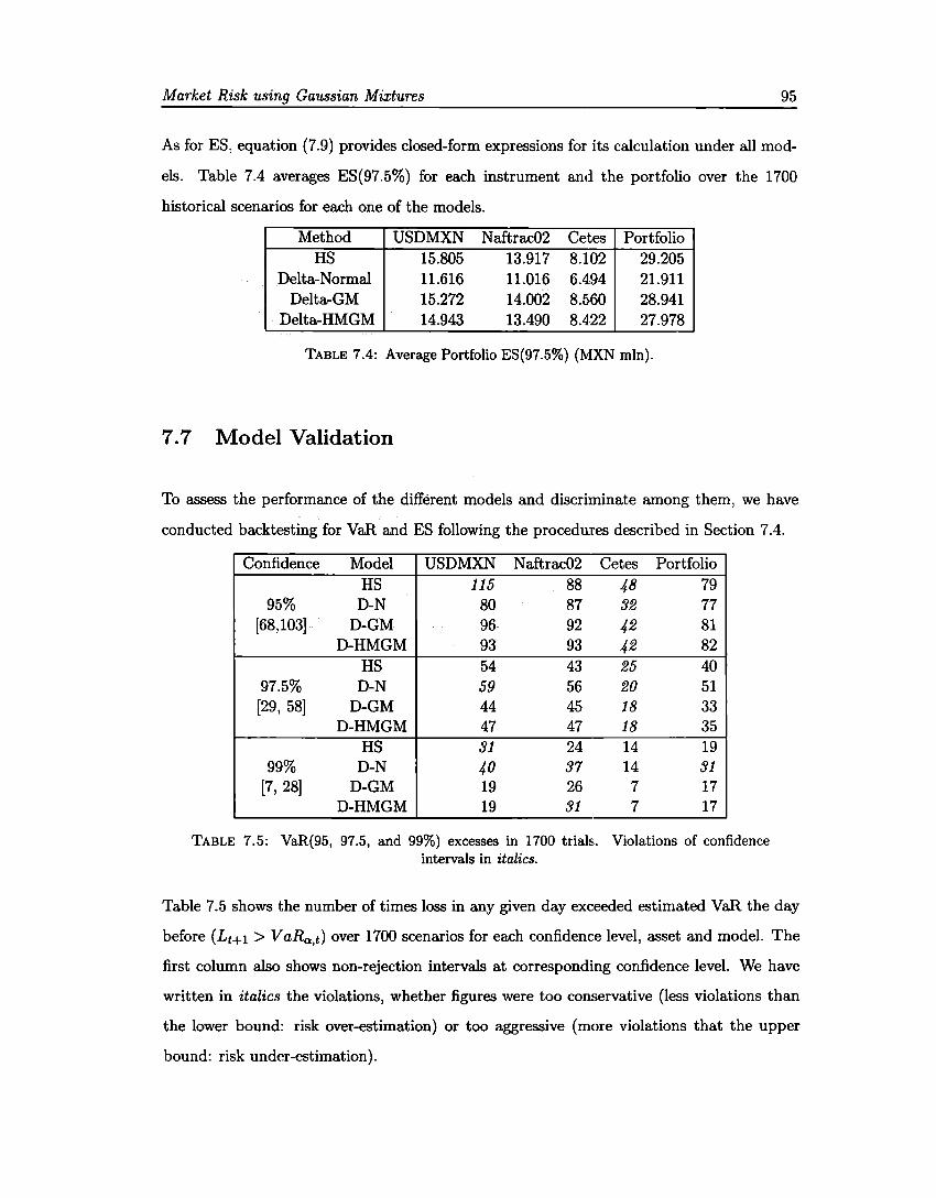
Market Risk using Gaussian Mixtures 95
As for ES, equation (7.9) provides closed-form expressions for its calculation under all mod
els. Table 7.4 averages ES{97.5%) for each instrument and the portfolio over the 1700
historical scenarios for each one of the models.
Method USDMXN Naftrac02 Cetes Portfolio HS 15.805 13.917 8.102 29.205
Delta-Normal 11.616 11.016 6.494 21.911 Delta-GM 15.272 14.002 8.560 28.941
Delta-HMGM 14.943 13.490 8.422 27.978
TABLE 7.4: Average Portfolio ES(97.5%) (MXN mln).
7. 7 Model Validation
To assess the performance of the different models and discriminate among them, we have
conducted backtesting for VaR and ES following the procedures described in Section 7.4.
Confidence Model USDMXN Naftrac02 Cetes Portfolio HS 115 88 48 79
95% D-N 80 87 32 77 [68,103] D-GM 96 92 42 81
D-HMGM 93 93 42 82 HS 54 43 25 40
97.5% D-N 59 56 20 51 [29, 58] D-GM 44 45 18 33
D-HMGM 47 47 18 35 HS 31 24 14 19
99% D-N 40 37 14 31 [7, 28] D-GM 19 26 7 17
D-HMGM 19 31 7 17
TABLE 7.5: VaR(95, 97.5, and 99%) excesses in 1700 trials.. Violations of confidence intervals in italics.
Table 7.5 shows the number of times loss in any given day exceeded estimated VaR the day
before ( Lt+l > V aRa,t) over 1700 scenarios for each confidence level, asset and model. The
first column also shows non-rejection intervals at corresponding confidence level. We have
written in italics the violations, whether figures were too conservative {less violations than
the lower bound: risk over-estimation) or too aggressive {more violations that the upper
bound: risk under-estimation).
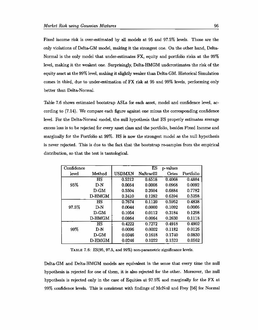
Market Risk using Gaussian Mixtures 96
Fixed income risk is over-estimated by all models at 95 and 97.5% levels. Those are the
only violations of Delta-GM model, making it the strongest one. On the other hand, Delta
Normal is the only model that under-estimates FX, equity and portfolio risks at the 99%
level, making it the weakest one. Surprisingly, Delta-HMGM underestimates the risk of the
equity asset at the 99% level, making it slightly weaker than Delta-GM. Historical Simulation
comes in third, due to under-estimation of FX risk at 95 ancl 99% levels, performing only
better than Delta-Normal.
Table 7 .6 shows estimated bootstrap ASLs for each asset, model and confidence level, ac
cording to (7.14). We compare each figure against one minus the corresponding confidence
level. For the Delta-Normal model, the null hypothesis that ES properly estimates average
excess loss is to be rejected for every asset class and the portfolio, besides Fixed Income and
marginally for the Portfolio at 99%. HS is now the strongest model as the null hypothesis
is never rejected. This is dueto the fact that the bootstrap re-samples from the empirical
distribution, so that the test is tautological.
Confidence ES p-values level Method USDMXN Naftrac02 Cetes Portfolio
HS 0.5212 0.6518 0.4068 0.4884 95% D-N 0.0054 0.0008 0.0968 0.0092
D-GM 0.5504 0.3904 0.6884 0.7782 D-HMGM 0.3410 0.1282 0.6394 0.5258
HS 0.7674 0.1120 0.5952 0.4838 97.5% D-N 0.0044 0.0000 0.1092 0.0066
D-GM 0.1054 0.0112 0.3184 0.1298 D-HMGM 0.0864 0.0064 0.2630 0.1118
HS 0.4222 0.7272 0.4918 0.4902 99% D-N 0.0096 0.0002 0.1182 0.0126
D-GM 0.0346 0.1618 0.1740 0.0830 D-HMGM 0.0246 0.1022 0.1522 0.0562
TABLE 7.6: ES(95, 97.5, and 99%) non-parametric significance levels.
Delta-GM and Delta-HMGM models are equivalent in the sense that every time the null
hypothesis is rejected for one of them, it is also rejected for the other. Moreover, the null
hypothesis is rejected only in the case of Equities at 97.5% and marginally for the FX at
99% confidence levels. This is consistent with findings of McNeil and Frey [56] for Normal
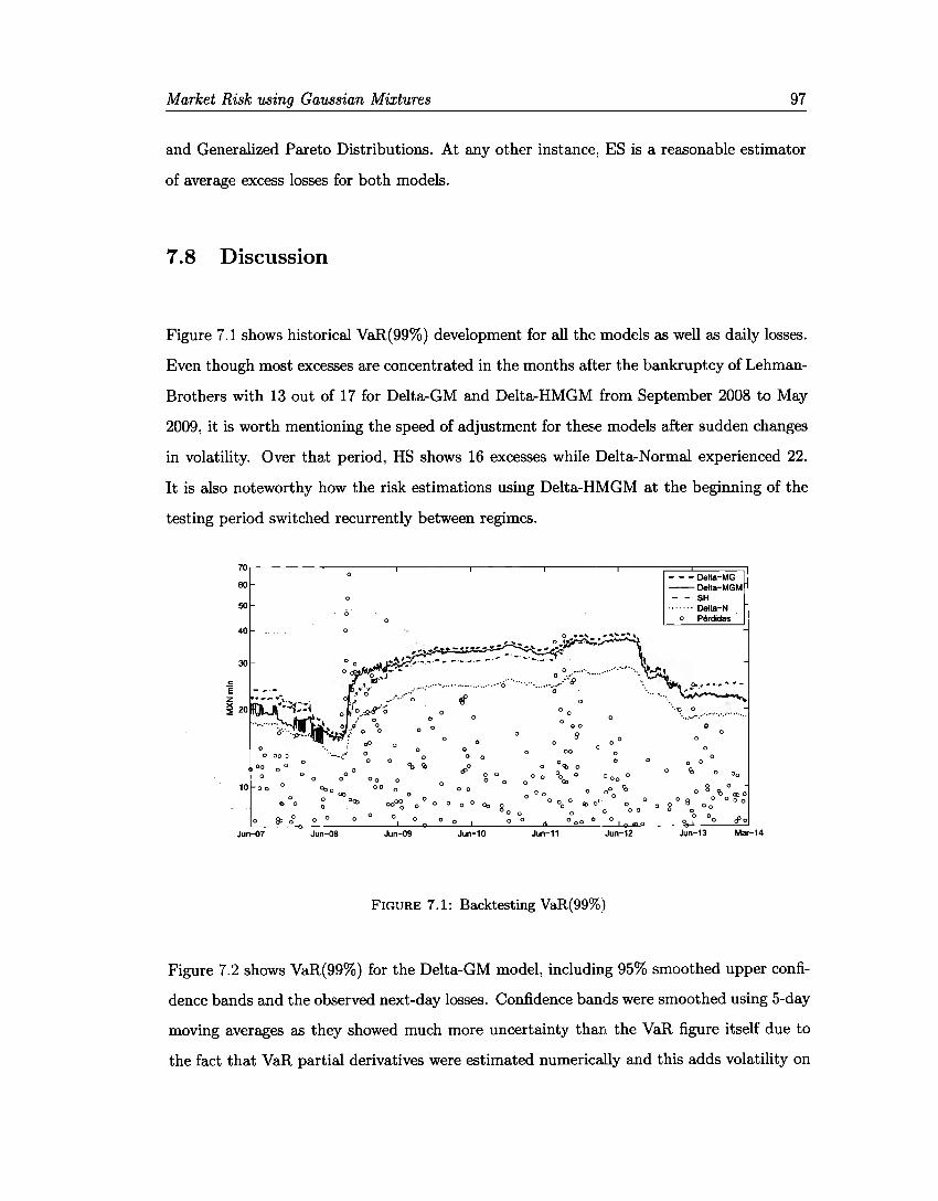
M arket Risk using Gaussian Mixtures 97
and Generalized Pareto Distributions. At any other instance, ES is a reasonable estimator
of average excess losses for both models.
7.8 Discussion
Figure 7.1 shows historical VaR(99%) development for all the models as well as daily losses.
Even though most excesses are concentrated in the months after the bankruptcy of Lehman
Brothers with 13 out of 17 for Delta-GM and Delta-HMGM from September 2008 to May
2009, it is worth mentioning the speed of adjustment for these models after sudden changes
in volatility. Over that period, HS shows 16 excesses while Delta-Normal experienced 22.
It is also noteworthy how the risk estimations using Delta-HMGM at the beginning of the
testing period switched recurrently between regimes.
e E
70 o
60
o 50
o o
40 o
30
o o ºº ::i
ºº o o o o
_. ............ _ •.••..••.••....••...•. ·¿,
.-· .. ····-,, i'
o
o o o
'b "'
o o
o o o o o o
o o o o o o ºº o
ºº o
cP o o o o
10 o o 0
Jun-07
o .. o
°"º 00 o º"' o
o o
Jun-08
o o
o o o o
ooº~o 00 o 0 eo o o o
Jun-09 Jun-10
o o o
00
El
o º~ o
o o
o o
- - - Delta-MG -- Delta-MGM - - SH
... · .. · Della-N o Pérdidas
··'0 o ·-... -..--.-··---···-·-·······
" o
o o 'o
o ºº o o o ºº0:1 o oºº o
o o o o oº o <o o 8 'o o co o
o ºo: ll> o''o ºo o o o 8 o 80 o oº o o o
o 00 o o O O ºo cPo
Jun-11 Jun-12 Jun-13 Mar-14
FIGURE 7.1: Backtesting VaR(99%)
Figure 7.2 shows VaR(99%) for the Delta-GM model, including 95% smoothed upper confi
dence bands and the observed next-day losses. Confidence bands were smoothed using 5-day
moving averages as they showed much more uncertainty than the VaR figure itself dueto
the fact that VaR partial derivatives were estimated numerically and this adds volatility on
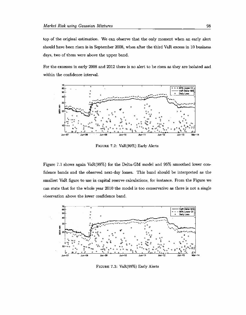
Market Risk using Gaussian Mixtures 98
top of the original estimation. We can observe that the only moment when an early alert
should have been risen is in September 2008, when after the third VaR excess in 10 business
days, two of them were above the upper band.
For the excesses in early 2008 and 2012 there is no alert to be risen as they are isolated and
within the confidence interval.
70 1 ----~----;0;---,-------,--------,-----,------;:::========:i
60 - - - 95% Upper CI so o --VaR Delle-MG
o , o Daily Loss 40 o
30
~ z o ~ 20 0 o o o o
o o o o o
o o o
o o o o o
OC·OO O O o
o o o ~ % ºº o o óP
o ·:> o o o oº o o o o o S o o o
o o o
o o o o ~ o ºº
10 o o ct>o 00
oo o o o O ºo g Oo:, oo0'i, O o O O O O O CQ
o o o o O 8
oQ:,o0
8' 0
o o o o o o o o 8 o "o o
o o o o o o o ::,
º 8 e ºº º 0 o cPo
Jun-07 Jun-08 Jun-09 Jun-10 Jun-11 Jun-12 Jun-13 Mar-14
FIGURE 7.2: VaR(99%) Early Ale:rts
Figure 7.:3 shows again VaR(99%) for the Delta-GM model and 95% smoothed lower con
fidence bands and the observed next-day losses. This band should be interpreted as the
smallest VaR figure to use in capital reserve calculations, for instance. From the Figure we
can state that for the whole year 2010 the model is too conservative as there is not a single
observation above the lower confidence band.
:,-----,-~0;,-----,-----,----~-----~---;::::_=.':...=v::::Ia=R=D=e=na=-=M=G;i
50 o - - - 95% Lower CI o
O o Oaily Loss
40 o ____ _,,...,_-...i..-:.~----~,-----30 o .... , ..... -,,,,,..,, .. .,,,-.,,- ..... ,,,.-..... 1
.. ., "\.¡ o o \ •• -~.. o ó> ""'"'
,. o o ré' o o , ' ..... , ... o oc9 o
O O O
o O O o\11ff'• 1
" t''""· 1
º ºo0 °"º º º º º º º º º ºeº º º º º º º ºo oo o o o o o oo o o
o~ o o : o oº o : o o o ~ ~ ; o% o o o o ~ ~ g o o: o o o ºq, o ºo oo
10 o o o et, o oO o o o o o o o o o o : i>º ººo ~ o o 8 o Q:, oº g> o
; ; o g o º: o c-o:'i, : o o o o o o o Co 8 g ºo o °o; o e o o o o o o 8 @ o go c9: Jun-07 Jun-08 Jun-09 Jun-10 Jun-11 Jun-12 Jun-13 Mar-14
FIGURE 7.3: VaR(99%) Early Alerts
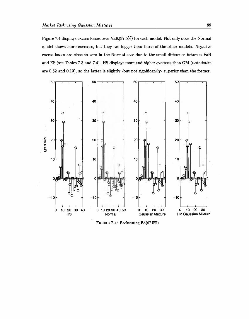
Market Risk using Gaussian Mixtures 99
Figure 7.4 displays excess losses over VaR(97.5%) for each model. Not only does the Normal
model shows more excesses, but they are bigger than those of the other models. Negative
excess losses are close to zero in the Normal case dueto the small difference between VaR
and ES (see Tables 7.3 and 7.4). HS displays more and higher excesses than GM (t-statistics
are 0.52 and 0.19), so the latter is slightly -but not significantly- superior than the former.
40
30
e E 20 z X ~
40 40
30 30
20 20
O 10 20 30 40 O 10 20 30 40 50 O 10 20 30 HS Normal Gaussian Mixture
FIGURE 7.4: Backtesting ES(97.5%)
O 10 20 30 HM Gaussian Mixture
Chapter 8
Conclusions
In this chapter we outline the main conclusions of the dissertation, organizing them into
three sections. In the first section we enumerate what we regard as the contributions of our
work. Then we draw sorne general conclusions about the methodology and the outcomes
based on the empirical results we have found. We finish sketching potential future research
on tapies we did not address either because they were not central or because they are beyond
the reach of our PhD project.
8.1 Contributions
Chapter 7 contains what we consider one of our main contributions, namely a closed-form
expression for the ES of a finite Gaussian Mixture distribution. Kamaruzzaman and Isa [41]
used a particular case of our expression, while Hardy [38] derived a specific expression for
the payment profile of European options. The simplicity of the formula is a confirmation of
the parsimony of the finite Gaussian Mixture model.
Another main contribution is also in Chapter 7 and we have called it Early Alerls. In tra
ditional model validation the risk manager has to wait to obtain a reasonably big sample
of risk estimates and next-day profit and loss figures in order to be able to make decisions
about the model. The idea behind our early alerts system is that this model validation
100
Conclusions 101
can be conducted from the very first day one estimates risk figures by constructing confi
dence intervals for those figures, as they are random variables, relying on the equivalence of
hypothesis testing and confidence intervals.
In Chapter 4 we extend the concept of persistence or expected duration of a state in a
hidden Markov model, to a set of states, or regime. This characteristic allows Markov
mixture distributions to capture asymmetry over time. This can be useful to estímate the
duration of a high volatility episode, for instance.
We have written a number of Matlab functions to accomplish the application of all the
reviewed methodologies: estimation, including standard errors, risk measurement and vali
dation. Among them, we want to highlight those that calculate standard errors for param
eter estimators under the information-based approach, as well as the bootstrap approach
for stationary and hidden Markov Gaussian Mixture models. None of them is part of the
current Statistics or Finance toolkits in Matlab.
The last -but not least- contribution is spread along the several chapters of this work. We
have gone over the full path, from parameter estimation, going through goodness of fit
testing and risk model estimation, up to model validation. We postulate that this should
be the standard approach to testing models, as it allows to identify the model strengths and
limitations.
In this fashion, we have contributed both to the theoretical ground as well as to the ap
plication field of the market risk discipline. This is in line with a personal belief that any
model should be precise enough to be trustworthy and reliable, while at the same time be
parsimonious enough to be applicable in real-life situations.
8.2 General Conclusions
In Chapter 6 we have shown evidence to state that the daily returns of the three market
risk factors under study are not properly described by the normal distribution. We consider
these results sufficient to justify the search of a more adequate model.

Conclusions 102
Attending to the methodology we postulate, we went through the process of parameter esti
mation (including standard errors calculation), goodness of fit testing, market risk measures
estimation ( again including standard errors) and model validation.
In the estimation step (Chapter 5) we have empirically verified that the finite Gaussian
Mixture model <loes not modify either the mass center or the dispersion of the returns joint
distribution, but only decomposes them into components, while showing higher kurtosis.
We also observed there that the stylized interpretation of the two component case holds:
one of the components describes the behaviour of the risk factor returns under the business
as usual regime, while the other component describes it under the stress regime. This allows
to model explicitly the covariance of the risk factor returns under each regime, which can
be useful for stress testing, for instance.
The above features also hold for the hidden Markov Gaussian mixture, with the additional
characteristic that it displays autocorrelation. However, in the case we studied, the ad
ditional parameter in the hidden Markov Gaussian mixture and, more importantly, the
associated increased estimation complexity do not seem to translate into a significantly
better model.
Allowing for autocorrelation, however, seems to have an advantage for the purpose of esti
mation: the distance among the means of the different components. They can be somewhat
close together and still be identifiable. In fact, for the same data set, estimated means
are closer under the hidden Markov model than they are under the stationary model. In
contrast, the graphical and moments methodologies reviewed, require that the component
means are well separated.
In the goodness of fit step (Chapter 6) we observed that a two-component Gaussian mixture
distribution looks asan adequate model for the returns of the FX rate and the equity returns,
but not for the interest rate returns.
Still, the fit is better with the two-component Gaussian mixture than it is with the normal
distribution, but not sufficient to pass the Kolmogorov-Smirnov test. The reason for this may
Conclusions 103
reside in the excess kurtosis not yet captured by a two-component model and the discrete
jumps observed in the empirical distribution. Including as many as 11 to 15 components in
the mixture is enough to pass the goodness of fit test, but this poses other questions, to be
addressed in the following section.
In this respect, the HM model is not superior to the stationary Gaussian Mixture model. The
reason seems to be that the Markov chain assumption <loes not provide enough flexibility to
capture the dynamics of the autocorrelation for the different risk factors at several lagged
periods.
After estimating market risk measures, in the model validation step {Chapter 7) we backtest
VaR calculations for several confidence levels and asset classes and found that the Gaussian
Mixture model performs better than the Delta-Normal and the Historical Simulation models,
failing only in the case of interest rates at 95 and 97 .5% confidence. Surprisingly, the Markov
Gaussian Mixture model underestimated the equity risk at 99%. lt is worth mentioning the
speed of adjustment of both mixture models after sudden changes in market volatility.
In the same chapter we backtest ES calculations for the same universe and found that
the stationary and Markov Gaussian Mixture models are both superior to Delta-Normal,
while they are equivalent among them, even though p-values for the markovian modelare
smaller, making the former slightly-but not significantly- superior than the latter. Historical
Simulation displays more and higher excesses than Gaussian Mixtures.
In summary, we believe that the application of a formal methodology that brings together
statistics and quantitative finance, has produced enough evidence to conclude that finite
Gaussian Mixtures should be considered as a serious candidate model for market risk as
sessment.
8.3 Future Research
The fact that the two-component Gaussian Mixture distribution <lid not pass the goodness
of fit test but adding 9 to 13 components makes the resulting distribution to pass the test

Conclusions 104
raises the question of how many components have to be added to the mixture distribution
in order to properly describe the data.
This is still pretty much an open question in mixture distributions that has been addressed
through the likelihood ratio, lnformation-based criteria (such as Akaike or Bayesian) and the
Bayesian estimation approach. We believe that there is room for contributing a goodness of
fit test that avoids the difficulties of dealing with the likelihood and makes use of the semi
parametric features of the mixture models to provide a guide to the number of components
to be included in the mixture.
Natural extensions in the application of the Gaussian Mixture model include asset classes,
number of factors and disciplines.
As far as asset classes is concerned, it can be used in the valuation and risk estimation of
assets where lack of symmetry is intrinsic, as it is the case of the volatility smile in options,
for instance.
With respect to number of factors (portfolio dimension, in financia! terms) it is yet to be
investigated if there is any relationship between the number of factors and their behaviour
and the number of components in the mixture. At the least, the questions of whether a high
dimension portfolio can be consistently estimated or if a reduction technique still allows the
intuitive interpretation of the model should be addressed.
Regarding disciplines, portfolio optimization is a potential field that can benefit from the
use of the Gaussian Mixture model, dueto two aspects: the well known sensitivity of port
folio weights to the covariance matrix of the assets that can be explicitly modeled through
different regimes, and the possibility of approximating an arbitrary distribution while pre
serving closedness under convolution and the parsimony in the estimation of quantiles and
tail expectations.
Finally, an additional step in the methodology we postulate is stress testing. Every model
should be tested under stressed conditions before being accepted. In the case of Gaussian

Conclusions 105
Mixtures, this type of testing is naturally captured in at least one component and should
be explored.
Appendix A
Proofs and Derivations
A.1 Convolution for Normal Distribution (Property 3.3).
If X,.._, Nd(µ,E) and l(x) = -(c+w'x), then l(X) ,.._, N(µ¡,cr¡), with µ¡ = -(c+w'µ) and
a¡= w 1
Ew.
Proof In a slightly more general context, let Y = WX + e, W E JR_kxd, e E IR.k, then the
characteristic function of Y is
1PY(t) E [eit'Y]
= E [ eit'(WX+c)]
eit'c1Px(W't)
eit'c exp { it'W µ - ~t'WI::W't} ,
where the last exponential is the characteristic function of the random vector X following a
normal distribution, evaluated at W't. Therefore
1PY(t) = exp { it'µ - ~t'Et},
106
Proofs and Derivations 107
which is again the characteristic function of a normal distribution with parameters µ, and
E, where µ,=e+ Wµ E JR.k and E= WEW' E JR.kxk_
Making k = 1 completes the proof of the Property, as in this case Y= -l(X), µ=e+ w' µ
and u2 = w'Ew. D
A.2 ES as Conditional Expectation (Proposition 7.4).
lf Lis continuous with distribution function FL and EILI < oo, then
ES0 = E[LIL ~ VaR0 ].
Proof. It is well-known that the random variable U= FL(L) follows a uniform distribution
on [O, 1] with density function fu(u) = 1, u E [O, 1]; therefore
¡1
VaRudu = fo1
VaRul(a,1)(u)fu(u)du
E [VaRu l(a,1) (U)] ,
where lA(·) is the indicator function of the set A. Using that VaRu = Fi 1(U) and that
continuity of FL implies that F¡; 1 is strictly increasing:
Dividing by 1 - o, we obtain:
E [ Fil (U)l( Fi1(a),Fi1 (1)) (Fil (U))]
E [Ll(VaRo,+oo)(L)] ·
-1
- r1vaRudu 1-o }
0
E [Ll{L>VaRo}]
P(L > VaR0 )
= E [LIL ~ VaR0 ]. (A.l)
Proofs and Derivations 108
o
A.3 ES for Normal Distribution.
Let L "' N (µ,o-2) and let q0 = VaR0 be the o-quantile of FL, i.e., FL(q0 ) = a. Let
h(·) = cp(·, µ, o-2 ) be the density function of L and let cp(·) =</>(·,O, 1) be the standard normal
density function with o-quantile equal to z0 . Using equation (7.4) and the distribution of
L, we have:
ES0 E [LI L 2'. qo] 1 1+00
= 1 _ o: ufL(u)du qo,_
- 1- ¡+oo ufL(u)du 1- o }qo.
1 ¡+oo 2 - -- u<f>( u,µ, u ) du,
1-o Qo.
with the change of variable u= uz + µ (z0 = qo.;µ, du = udz):
= - 1- ¡+oo (zu + µ) <f>(z)dz 1 - O Ízo.
= 1 ~ 0 [u 1:00
z<f>(z)dz + µ 1:XJ </>(z)dz]
= 1 ~ 0 [-u<f>(z) + µcI>(z)]l;o.00
1 = l _ 0
[uef>(z0 ) + µ (l - cl>{z0 ))]
= 1 ~
0 [ u<f> ( cI>- 1 (a)) + µ ( 1 - o)]
µ + l: o</> (cI>-l(o:)).
(A.2)
(A.3)
Appendix B
Matlab Code
B.1 VaR and ES for Gaussian Mixtures
function [VaR,ES] = GaussianMixtureRisk(GMdist,alph.a)
% Returns a dx2 matrix containing VaR and ES calculated using
% Gaussian Mixture distribution object GMdist,
% if it is multidimensional, risk is calculated on each dimension;
% alpha is an optional argument (scalar or vector)
% with confidence level(s).
if nargin < 2
alpha = [0.99 0.975]; % Basel III VaR and ES conf levels as default
else
if size(alpha)==1 alpha = [alpha alpha];
end
VaR = nan(GMdist.NDimensions,1);
ES= nan(GMdist.NDimensions,1);
for j = 1:GMdist.NDimensions
% Create unidimensional Gaussian Mixture distribution
% object using parameter passed to the function
mu= GMdist.mu(:, j);
109
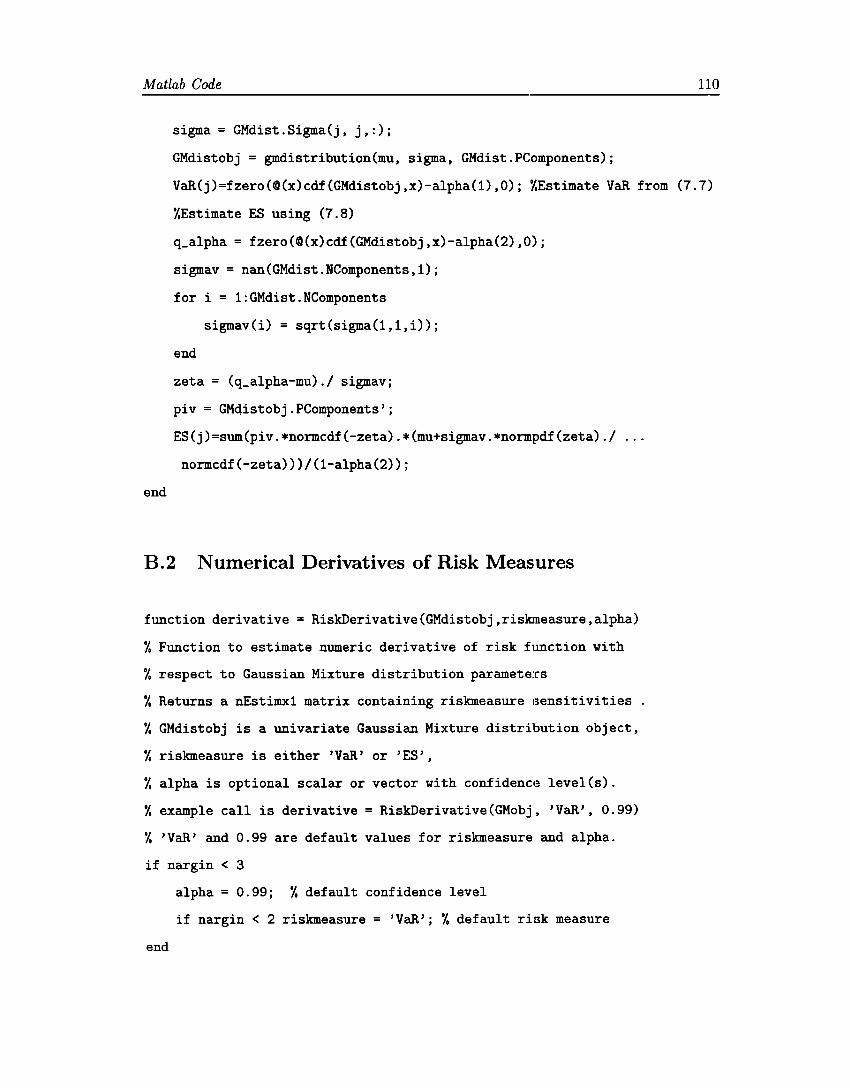
Matlab Code 110
sigma= GMdist.Sigma(j, j,:);
GMdistobj = gmdistribution(mu, sigma, GMdist.PComponents);
VaR(j)=fzero(©(x)cdf(GMdistobj,x)-alpha(1),0); %Estímate VaR from (7.7)
%Estímate ES using (7.8)
end
q_alpha = fzero(©(x)cdf(GMdistobj,x)-alpha(2),0);
sigmav = nan(GMdist.NComponents,1);
for i = 1:GMdist.NComponents
sigmav(i) = sqrt(sigma(1,1,i));
end
zeta= (q_alpha-mu)./ sigmav;
piv = GMdistobj.PComponents';
ES(j)=sum(piv.*normcdf(-zeta).*(mu+sigmav.*normpdf(zeta)./
normcdf(-zeta)))/(1-alpha(2));
B.2 Numerical Derivatives of Risk Measures
function derivative = RiskDerivative(GMdistobj,riskmeasure,alpha)
% Function to estímate numeric derivative of risk f1mction with
o/, respect to Gaussian Mixture distribution paramete:rs
% Returns a nEstimx1 matrix containing riskmeasure :sensitivities
% GMdistobj is a univariate Gaussian Mixture distribution object,
% riskmeasure is either 'VaR' or 'ES',
% alpha is optional scalar or vector with confidence level(s).
% example call is derivative = RiskDerivative(GMobj, 'VaR', 0.99)
% 'VaR' and 0.99 are default values for riskmeasure and alpha.
if nargin < 3
alpha = 0.99; % default confidence level
if nargin < 2 riskmeasure = 'VaR'; % default risk measure
end

Matlab Code
o/. obtain additional parameters
g=GMdistobj.NComponents;
nEstim = g-1 + g + g;
o/. allocate memory
derivativa= nan(g-1 + g + g,1);
x = nan(1,2);
VaR = nan(1,2);
ES= nan(1,2);
o/. build estimators vector
estimators = cat(2, GMdistobj.PComponents(1:g-1),
reshape(GMdistobj .mu', 1,g), reshape(GMdistobj. Sigma., 1,g));
for k = 1:nEstim
delta= min(1e-6,abs(estimators(k))/2);
for j =1:2
estim = estimators(k); o/. record value of estimator to modify
x(j)=estimators(k) + (-1)-j * delta; o/. prepare jth point to eval
estimators(k)=x(j);
o/. construct gm object with modified estimator
pi= [estimators(1:g-1) 1-sum(estimators(1:g-1))];
mu= reshape(estimators(g:2*g-1),g,1);
sigma= reshape(estimators(2*g:3*g-1),1,1,g);
gmdelta = gmdistribution(mu, sigma, pi);
111
[VaR(j) ES(j)] = GaussianMixtureRisk(gmdelta,alpha); o/. jth f value
estimators(k)=estim; o/. restore value of estimator vector
end
o/. decide which risk measure to use
if strcmpi(riskmeasure,'VaR')
y= [VaR(1) VaR(2)];
else
y= [ES(1) ES(2)];
end
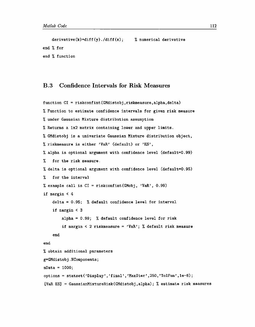
Matlab Code
derivative(k)=diff(y)./diff(x);
end % for
end % function
% numerical derivativa
B.3 Confidence Intervals for Risk Measures
function CI = riskconfint(GMdistobj,riskmeasure,alpha,delta)
% Function to estimate confidence intervals for given risk measure
o/, under Gaussian Mixture distribution assumption
% Returns a 1x2 matrix containing lover and upper limits.
% GMdistobj is a univariate Gaussian Mixture distribution object,
% riskmeasure is either 'VaR' (default) or 'ES',
% alpha is optional argument vith confidence level (default=0.99)
% for the risk measure.
% delta is optional argument vith confidence level (default=0.95)
% for the interval
% example call is CI = riskconfint(GMobj, 'VaR', 0.~l9)
if nargin < 4
delta= 0.95; % default confidence level for interval
if nargin < 3
end
end
alpha = 0.99; % default confidence level for risk
if nargin < 2 riskmeasure = 'VaR'; % default risk measure
% obtain additional parameters
g=GMdistobj.NComponents;
nData = 1000;
options = statset('Display', 'final', 'Maxiter' ,250, 'TolFun' ,1e-6);
112
[VaR ES]= GaussianMixtureRisk(GMdistobj,alpha); % estimate risk measures
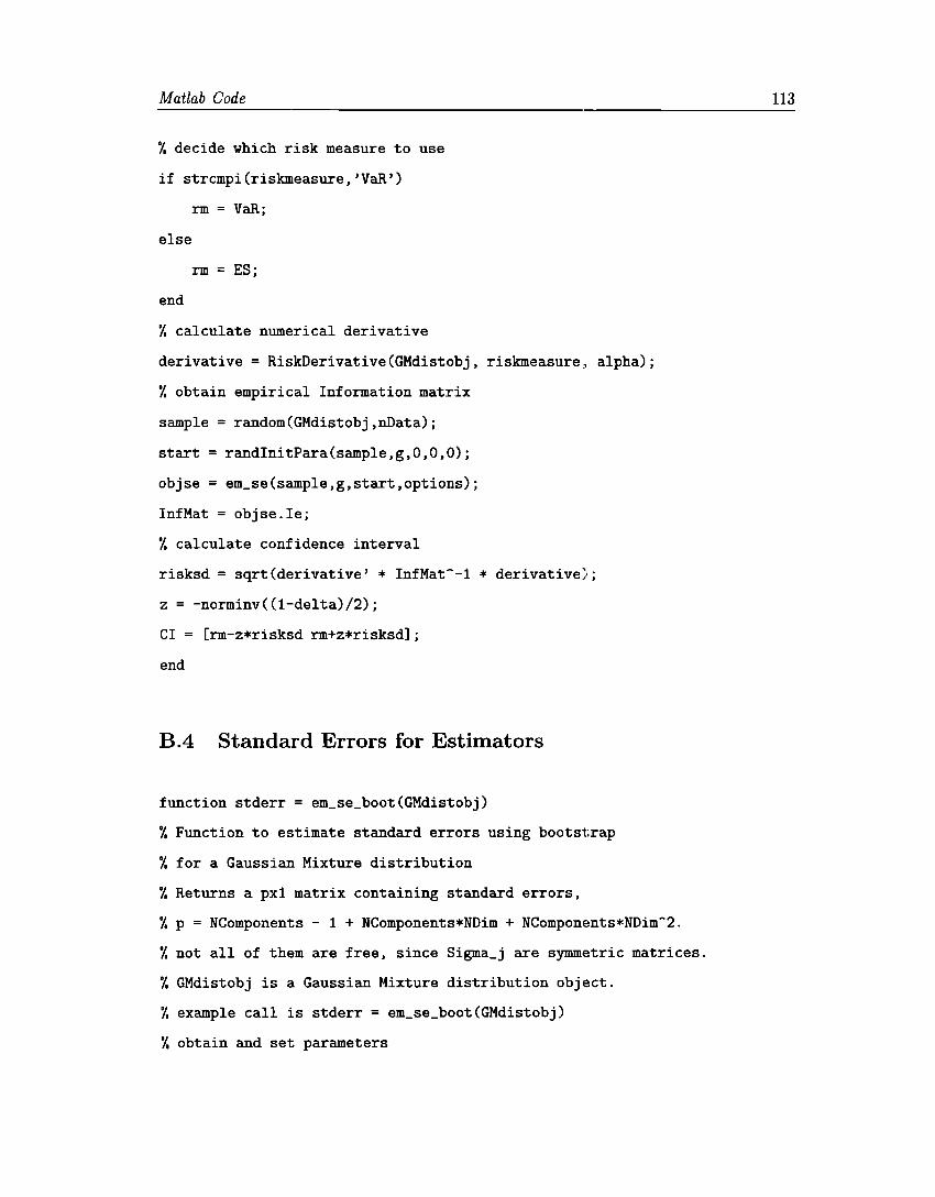
Matlab Code
% decide which risk measure to use
if strcmpi(riskmeasure,'VaR')
rm = VaR;
else
rm = ES;
end
% calculate numerical derivative
derivative = RiskDerivative(GMdistobj, riskmeasure, alpha);
% obtain empirical Information matrix
sample = random(GMdistobj,nData);
start = randinitPara(sample,g,0,0,0);
objse = em_se(sample,g,start,options);
InfMat = objse.Ie;
% calculate confidence interval
risksd = sqrt(derivative' * InfMat--1 * derivative);
z = -norminv((l-delta)/2);
CI = [rm-z*risksd rm+z*risksd];
end
B .4 Standard Errors for Estimators
function stderr = em_se_boot(GMdistobj)
% Function to estimate standard errors using bootstrap
% for a Gaussian Mixture distribution
% Returns a px1 matrix containing standard errors,
% p = NComponents - 1 + NComponents*NDim + NComponents*NDim-2.
% not all of them are free, since Sigma_j are symmetric matrices.
% GMdistobj is a Gaussian Mixture distribution object.
% example call is stderr = em_se_boot(GMdistobj)
% obtain and set parameters
113
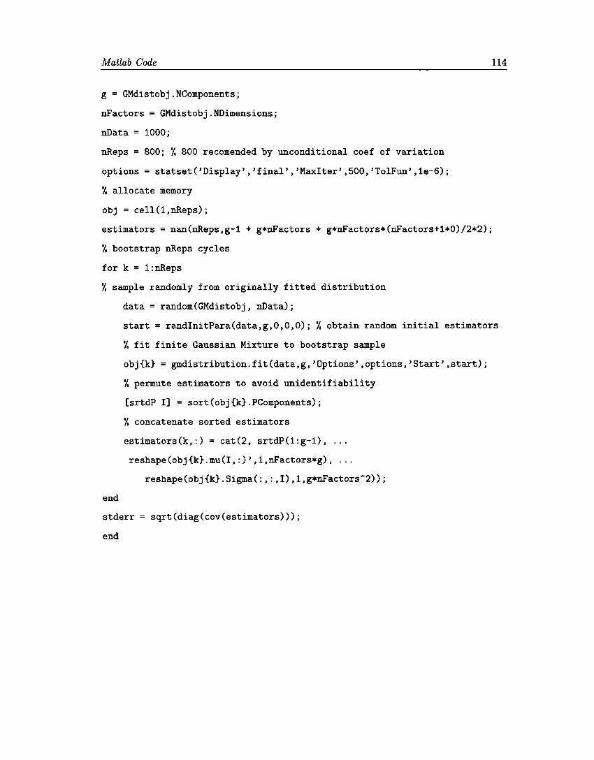
Matlab Code
g = GMdistobj.NComponents;
nFactors = GMdistobj.NDimensions;
nData = 1000;
nReps = 800; % 800 recomended by unconditional coef of variation
options = statset('Display','final','Maxiter',500,'TolFun',1e-6);
% allocate memory
obj = cell(1,nReps);
estimators = nan(nReps,g-1 + g*nFactors + g*nFactors*(nFactors+l*0)/2*2);
% bootstrap nReps cycles
for k = 1 :nReps
% sample randomly from originally fitted distribution
data= random(GMdistobj, nData);
114
start = randinitPara(data,g,0,0,0); % obtain random initial estimators
% fit finite Gaussian Mixture to bootstrap sample
obj{k} = gmdistribution.fit(data,g,'0ptions',options,'Start',start);
% permute estimators to avoid unidentifiability
[srtdP I] = sort(obj{k}.PComponents);
% concatenate sorted estimators
estimators(k,:) = cat(2, srtdP(l:g-1),
reshape(obj{k}.mu(I,:)',1,nFactors*g), ...
reshape(obj{k}.Sigma(:,:,I),1,g*nFactors-2));
end
stderr = sqrt(diag(cov(estimators)));
end
Bibliography
[1] ACERBI, C., AND TASCHE, D. On the coherence of expected shortfall. Journal of
Banking & Finance 26, 7 (July 2002), 1487-1503.
[2] ALEXANDER, C., AND LAZAR, E. Normal mixture GARCH{l,l): Applications to
exchange rate modelling. Journal of Applied Econometrics 21, 3 {2006), 307-336.
[3] ANDERSON, T., AND DARLING, D. A test of goodness of fit. J. Am. Stat. Assoc. 49
{1954), 765-769.
[4] ARTZNER, P., DELBAEN, F., EBER, J. M., AND HEATH, D. Coherent measures of
risk. Math. Finance 9, 3 {1999), 203-228.
[5] ASMUSSEN, S. R. Steady-state properties of GI/G/1. In Applied Probability and
Queues, vol. 51 of Stochastic Modelling and Applied Probability. Springer New York,
2003, pp. 266-301.
[6] BASEL COMMITTEE ON BANKING SUPERVISION. Basel Ill: A global regulatory
framework for more resilient banks and banking systems, 2011.
[7] BASEL COMMITTEE ON BANKING SUPERVISION. Fundamental review of the trading
book: A revised market risk framework, 2013.
[8] BAUM, L., AND EAGON, J. An inequality with applications to statistical estimation
for probabilistic functions of Markov processes and to a model for ecology. Bull. A m.
Math. Soc. 73 {1967), 360-363.
[9] BAUM, L., AND PETRIE, T. Statistical inference for probabilistic functions of finite
state Markov chains. Ann. Math. Stat. 37 {1966), 1554-lfi63.
115
Bibliography 116
[10] BAUM, L., PETRIE, T., SOULES, G., AND WEISS, N. A maximization technique
occurring in the statistical analysis of probabilistic functions of Markov chains. Ann.
Math. Stat. 41 {1970), 164-171.
[11] BEHR, A., AND POETTER, U. Modeling Marginal Distributions of Ten European
Stock Market lndex Returns. International Research Journal of Finance and
Economics, 28 (2009), 104-119.
[12] BHATTACHARYA, C. G. A simple method of resolution of a distribution into gaussian
components. Biometrics 23, 1 (1967), 115-135.
[13] BLACK, F., AND SCHOLES, M. S. The pricing of options and corporate liabilities.
Journal of Political Economy 81, 3 (1973), 637-654.
[14] BOYO, S., AND VANDENBERGHE, L. Convex Optimization. Berichte über verteilte
messysteme. Cambridge University Press, 2004.
[15] CAMPBELL, S. D. A review of backtesting and backtesting procedures. Journal of
Risk (2007).
[16] CASELLA, G. Refining binomial confidence intervals. Can. J. Stat. 14 (1986),
113-129.
[17] CASELLA, G., AND BERGER, R. L. Statistical inference. Pacific Grove, CA:
Wadsworth & Brooks/Cole Advanced Books & Software, 2002.
[18] CHARLIER, C. V. L. Researches into the theory of probability. Lund Univ. Arsskr.,
51 S. 4º. u. 7 Taf., 1906.
[19] COMISIÓN NACIONAL BANCARIA Y DE VALORES. General dispositions applicable to
credit institutions {in spanish). Available at www.cnbv.gob.mx, 2005.
[20] CRAWFORD, S. L. An application of the Laplace method to finite mixture
distributions. J. Am. Stat. Assoc. 89, 425 {1994), 259-267.
[21] CUEVAS, C., ÍÑIGO, J., AND ROSALES, J. Statistical modeling of the distribution of
financia! returns. Available at spitswww.uvt.nl/fsw/mto/IFCS2013, 2013.
Bibliography 117
[22] CUEVAS, C., ANO ROSALES, J. Gaussian mixtures and financial returns. Available at
www.actuaries.org/mexico2012/abstracts/, 2012.
[23] DEMPSTER, A., LAIRO, N., ANO RUBIN, D. Maximum likelihood from incomplete
data via the EM algorithm. Discussion. J. R. Stat. Soc., Ser. B 39 (1977), 1-38.
[24] EFR0N, B., ANO HINKLEY, D. V. Assessing the accuracy of the maximum likelihood
estimator: observed versus expected Fisher information. Biometrika 65 (1978),
457-487.
[25] EFR0N, B., ANO TIBSHIRANI, R. J. An introduction to the bootstrap. New York, NY:
Chapman & Hall, 1994.
[26] ENGEL, C., ANO HAMILT0N, J. D. Long Swings in the Dollar: Are they in Data and
do Markets Know it? American Economic Review 80 (1990), 689-713.
[27] EscH, D. N. Non-normality facts and fallacies. Journal of lnvestment Management
8, 1 (2010), 49-61.
[28] EVERITT, B. S., ANO HANO, D. Finite mixture distributions. New York, NY:
Chapman & Hall, 1981.
[29] FAMA, E. F. The behavior of stock-market prices. Joumal of Business 38, 1 (1965),
34-105.
[30] FAMA, E. F., ANO FRENCH, K. R. The Capital Asset Pricing Model: Theory and
Evidence. Journal of Economic Perspectives, American Economic Association 18, 3
(2004), 25-46.
[31] FANG, KAITAI, K. S., ANO Na, K. W. Symmetric mu.ltivariate and related
distributions. Monographs on statistics and applied probability. Chapman and Hall,
1990.
[32] FELLER, W. On a general class of "contagious" distributions. Ann. Math. Stat. 14
(1943), 389-400.
Bibliography
[33] FRANCQ, C., AND ZAKOIAN, J.-M. Linear-representations based estimation of
switching-regime garch models. Working Papers 99-57, Centre de Recherche en
Economie et Statistique, 1999.
118
[34] FRÜHWIRTH-SCHNATTER, S. Finite mixture and Markov switching models. Berlín:
Springer, 2006.
[35] GRZENDA, W., AND ZIEBA, W. Conditional central limit theorem. Int. Math. Forum
3, 29-32 (2008), 1521-1528.
[36] HAAS, M., MITTNIK, S., AND PAOLELLA, M. S. Mixed normal conditional
heteroskedasticity. Journal of Financial Econometrics 2, 2 (2004), 211-250.
[37] HAMILTON, J. Chapter 50 State-space models. Handbook of Econometrics 4 (1994),
3039-3080.
[38] HARDY, M. R. A regime-switching model of long-term stock returns. N. Am. Actuar.
J. 5, 2 (2001), 41-53.
[39] JARQUE, C. M., AND BERA, A. K. A test for normality of observations and
regression residuals. Int. Stat. Rev. 55 (1987), 163-172.
[40] KAMARUZZAMAN, ZETTY AIN, I. z., AND !SMAIL, M. T. Mixtures of normal
distributions: Application to bursa malaysia stock market indices. World Applied
Sciences Journal 16, 6 (2012), 781-790.
[41] KAMARUZZAMAN, Z. A., AND ISA, Z. Estimation of value at risk and conditional
value at risk using normal mixture distributions model. AIP Conference Proceedings
1522, 1 (2013).
[42] KIM, C.-J. Dynamic linear models with markov-switching. Journal of Econometrics
60, 1-2 (1994), 1-22.
[43] KLUGMAN, S. A., PANJER, H. H., AND WILLMOT, G. E. Loss models. From data to
decisions., 4th revised and updated ed. ed. Hoboken, NJ: John Wiley & Sons, 2012.
Bibliography 119
[44] KUPIEC, P. H. Techniques for Verifying the Accuracy of Risk Measurement Models.
The Journal of Derivatives 3, 2 (1995), 73-84.
[45] LEE, S. X., AND McLACHLAN, G. J. Modelling asset return using multivariate
asymmetric mixture models with applications to estimation of value at risk. In
Piantadosi, J., Anderssen, R.S. and Boland J. {eds) MODSIM2013, 20th
International Congress on Modelling and Simulation. (2013), 1228-1234.
[46] LER0UX, B. G., AND PUTERMAN, M. L. Maximum-penalized-likelihood estimation
for independent and markov-dependent mixture models. Biometrics (1992), 545-558.
[47] LILLIEF0RS, H. W. On the kolmogorov-smirnov tests for normality with mean and
variance unknown. Journal of the American Statistical Association 62 (1967),
399-402.
[48] LINDSAY, B. G. Moment matrices: Applications in mixtures. Ann. Stat. 17, 2 (1989),
722-740.
[49] LINDSAY, B. G., AND BASAK, P. Multivariate normal mixtures: A fast consistent
method of moments. J. Am. Stat. Assoc. 88, 422 (1993), 468-476.
[50] LINTNER, J. The valuation of risk assets and the selection of risky investments in
stock portfolios and capital budgets. Review of Economics and Statistics 47, 1 (1965),
13-37.
{51] L0PEZ DE PRADO, M., AND FOREMAN, M. D. A mixture of gaussians approach to
mathematical portfolio oversight: the ef3m algorithm. Quantitative Finance 14, 5
(2014), 913-930.
[52] MARK0WITZ, H. M. Selected works. Edited by Harry M. Markowitz. Hackensack, NJ:
World Scientific, 2008.
[53] McLACHLAN, G., AND PEEL, D. Finite mixture models. Chichester: Wiley, 2000.
[54] McLACHLAN, G. J., AND BASF0RD, K. E. Mixture models: inference and
applications to clustering. New York, NY: Marcel Dekker, lnc., 1988.
Bibliography
[55] McLACHLAN, G. J., AND KRISHNAN, T. The EM algorithm and extensions., 2nd
ed. ed. Hoboken, NJ: John Wiley & Sons, 2008.
120
[56] MCNEIL, A. J., AND FREY, R. Estimation of tail-related risk measures for
heteroscedastic financial time series: an extreme value approach. Journal of Empirical
Finance 7, 3-4 {2000), 271-300.
[57] McNEIL, A. J., FREY, R., AND EMBRECHTS, P. Quantitative risk management.
Concepts, techniques, and tools. Princeton, NJ: Princeton University Press, 2005.
[58] MEILIJSON, l. A fast improvement to the EM algorithm. on its own terms. J. R. Stat.
Soc., Ser. B 51, 1 {1989), 127-138.
[59] MEUCCI, A. Risk and asset allocation. , corrected 3rd printing ed. Springer, Berlin,
2009.
[60] MICHAUD, R. 0., AND MICHAUD, R. 0. Efficient Asset Management: A Practical
Cuide to Stock Portfolio Optimization and Asset Allocation, 2nd ed. Oxford
University Press, USA, 2008.
[61] PAGAN, A. R., AND SCHWERT, G. W. Alternative models for conditional stock
volatility. Journal of Econometrics 45, 1-2 {1990), 267-290.
[62] PEARSON, K. Contributions to the mathematical theory of evolution. Philos. Trans.
R. Soc. Lond., A 185 {1894), 71-110.
[63] PENNACCHI, G. G. Theory of Asset Pricing. Addison-Wesley series in finance.
Pearson/ Addison-Wesley, 2008.
[64] QUANDT, R. E., AND RAMSEY, J. B. Estimating mixtures of normal distributions
and switching regressions. J. Am. Stat. Assoc. 73 {1978), 730-752.
[65] RABINER, L. R. A tutorial on hidden Markov models and selected applications in
speech recognition. Proceedings of the IEEE 77, 2 {1989), 257-286.
[66] REDNER, R. A., AND WALKER, H. F. Mixture densities, maximum likelihood and
the EM algorithm. SIAM Rev. 26 {1984), 195-239.
Bibliography
[67] ROSALES, J. Finite gaussian mixtures and market risk management (in Spanish),
2014.
121
[68] ROSALES, J. Market risk mea.sures using finite gaussian mixtures. Journal of Applied
Finance and Banking 4, 6 (2014), 29-45.
[69] ROSENBERG, B. Extra-market components of covariance in security returns. Journal
of Financia[ and Quantitative Analysis 9 (3 1974), 263-274.
[70] Ross, S. M. Introduction to probability models., 11th ed. ed. Amsterdam:
Elsevier/ Academic Press, 2014.
[71] RYDÉN, TOBIAS, T. T., AND ASBRINK, s. Stylized facts of daily return series and
the hidden markov model. Journal of Applied Econometrics 13, 3 (1998), 217-244.
[72] ScLOVE, S. L. Time-series segmentation: A model anda method. Jnf. Sci. 29
(1983), 7-25.
[73] SEIDEL, W., MOSLER, K., AND ALKER, M. Likelihood ratio tests based on
subglobal optimization: A power comparison in exponential mixture models. Stat.
Pap. 41, 1 {2000), 85-98.
[74] SENIOR SUPERVISORS GROUP. Observations on risk management practices during the
recent market turbulence, Oct 2008.
[75] SHARPE, W. F. Capital asset prices: A theory of market equilibrium under
conditions of risk. The Journal of Finance 19, 3 (1964), 425-442.
[76] STEPHENS, M. A. Edf statistics for goodness of fit and sorne comparisons. Journal of
the American Statistical Association 69, 347 (1974), 730--737.
[77] TAN, K., AND CHU, M. Estimation of portfolio return and value at risk using a class
of gaussian mixture distributions. The International Journal of Business and Finance
Research 6, 1 (2012), 97-107.
[78] TEICHER, H. On the mixture of distributions. Ann. Math. Stat. 31 (1960), 55-73.
[79] TEICHER, H. ldentiability of finite mixtures. Ann. Math. Stat. 34 (1963), 1265-1269.
Bibliogmphy 122
[80] THEODOSSIOU, P. Skewed generalized error distribution of financial assets and option
pricing, 2000.
[81] TITTERINGTON, D., SMITH, A., AND MAKOV, u. Statistical analysis of finite
mixture distributions. 1985.
[82] TURNER, T. ROLF, C. M. A., AND THOMSON, P. J. Hidden markov chains in
generalized linear models. Canadian Joumal of Statistics 26, 1 (1998), 107-125.
[83] YAKOWITZ, s., AND SPRAGINS, J. On the identifiability of finite mixtures. Ann.
Math. Stat. 39 (1968), 209-214.
[84] YooN, S. M., AND KANG, S. H. A skewed student-t vaJue-at-risk approach for long
memory volatility processes in japanese financial markets. Joumal of Intemational
Economic Studies 11, 1 (2007), 211-242.
[85] ZHANG, M.-H., AND CHENG, Q.-S. An approach to va:r for capital markets with
gaussian mixture. Applied mathematics and computation 168, 2 (2005), 1079-1085.


![Approximate Inference for Deep Latent Gaussian …enalisni/BDL_paper20.pdf · Approximate Inference for Deep Latent Gaussian Mixtures ... Burda et al. [2] proposed an importance weighted](https://img.pdfslide.us/doc/110x75/5b68fe837f8b9a6f778d7757/approximate-inference-for-deep-latent-gaussian-enalisnibdl-approximate-inference.jpg)