Gaussian process regression

Bernád Emőke

2007

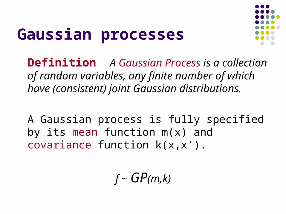
Gaussian processes

Definition A Gaussian Process is a collection of random variables, any finite number of which have (consistent) joint Gaussian distributions.

A Gaussian process is fully specified by its mean function m(x) and covariance function k(x,x’).

f ~ GP(m,k)

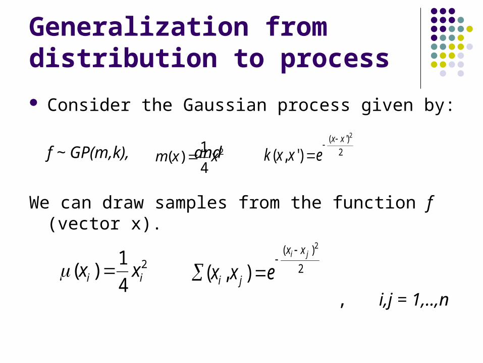
Generalization from distribution to process

Consider the Gaussian process given by:

f ~ GP(m,k), and

We can draw samples from the function f (vector x).

, i,j = 1,..,n

2

4

1)( xxm 2

)'( 2

)',(xx

exxk

2

4

1)( ii xx 2

)( 2

),(ji xx

ji exx

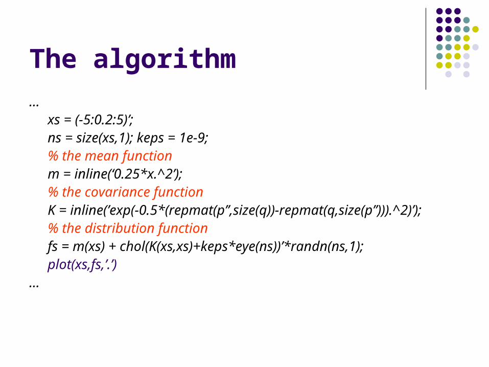
The algorithm

…xs = (-5:0.2:5)’; ns = size(xs,1); keps = 1e-9;% the mean functionm = inline(‘0.25*x.^2’);% the covariance functionK = inline(’exp(-0.5*(repmat(p’’,size(q))-repmat(q,size(p’’))).^2)’);% the distribution functionfs = m(xs) + chol(K(xs,xs)+keps*eye(ns))’*randn(ns,1);plot(xs,fs,’.’)

…

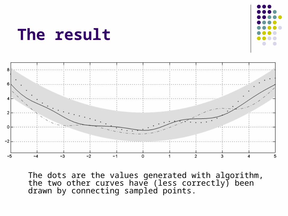
The result

The dots are the values generated with algorithm, the two other curves have (less correctly) been drawn by connecting sampled points.

Posterior Gaussian Process The GP will be used as a prior for Bayesian inference. The primary goals computing the posterior is that it can be used to

make predictions for unseen test cases. This is useful if we have enough prior information about a dataset

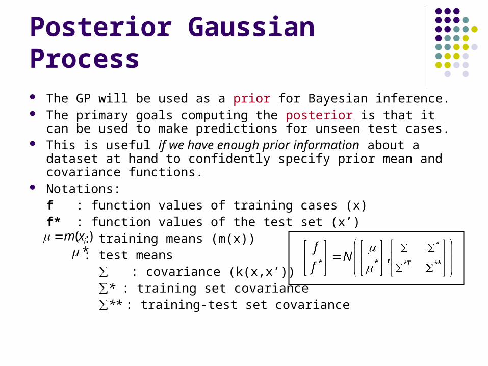
at hand to confidently specify prior mean and covariance functions. Notations:

f : function values of training cases (x)f* : function values of the test set (x’)

: training means (m(x)) : test means

∑ : covariance (k(x,x’)) ∑* : training set covariance ∑** : training-test set covariance

)( ixm*

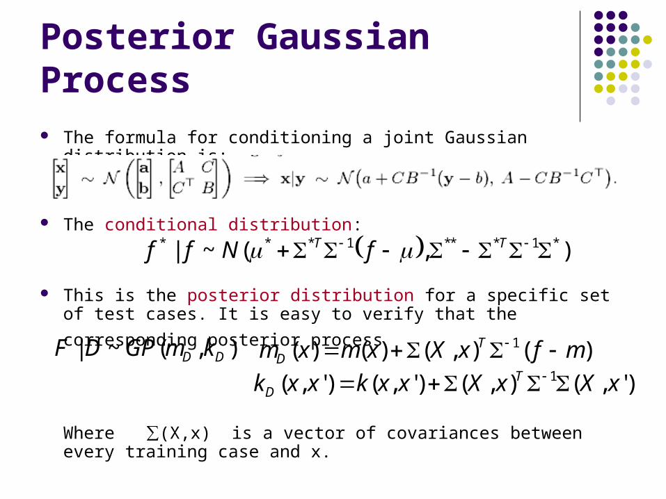
Posterior Gaussian Process The formula for conditioning a joint Gaussian distribution is:

The conditional distribution:

This is the posterior distribution for a specific set of test cases. It is

easy to verify that the corresponding posterior process

Where ∑(X,x) is a vector of covariances between every training case and x.

),(~| *1***1*** TT fNff

),(~| DD kmGPDF )(),()()( 1 mfxXxmxm TD

)',(),()',()',( 1 xXxXxxkxxk TD

Gaussian noise in the training outputs

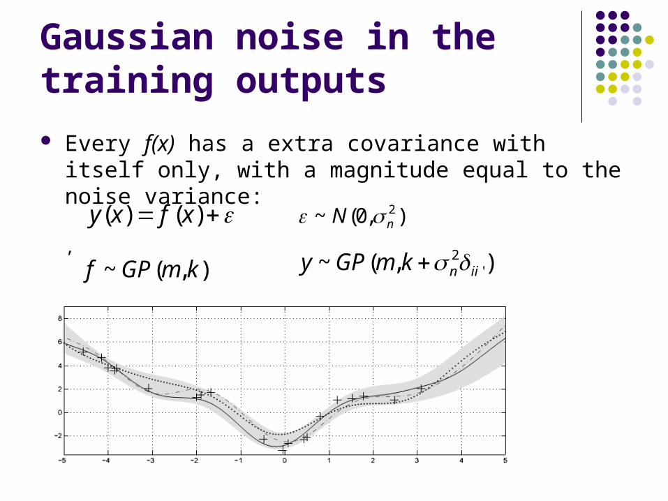
Every f(x) has a extra covariance with itself only, with a magnitude equal to the noise variance:

,

,

20 training data

GP posterior

noise level 0,7

)()( xfxy ),0(~ 2nN

),(~ kmGPf ),(~ '2iinkmGPy

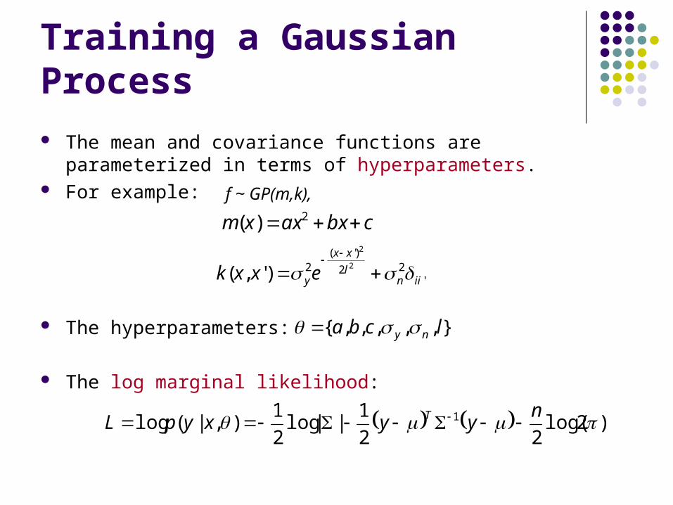
Training a Gaussian Process The mean and covariance functions are parameterized in terms of

hyperparameters. For example:

The hyperparameters:

The log marginal likelihood:

cbxaxxm 2)(

f ~ GP(m,k),

'22

)'(2 2

2

)',( iinl

xx

yexxk

},,,,,{ lcba ny

)2log(22

1||log

2

1),|(log 1 n

yyxypL T

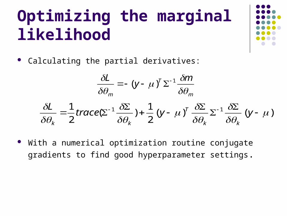
Optimizing the marginal likelihood Calculating the partial derivatives:

With a numerical optimization routine conjugate gradients to find good

hyperparameter settings.

m

T

m

my

L

1)(

)()(2

1)(

2

1 11

yytraceL

kk

T

kk

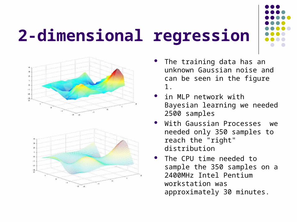
2-dimensional regression The training data has an unknown

Gaussian noise and can be seen in the figure 1.

in MLP network with Bayesian learning we needed 2500 samples

With Gaussian Processes we needed only 350 samples to reach the "right" distribution

The CPU time needed to sample the 350 samples on a 2400MHz Intel Pentium workstation was approximately 30 minutes.

References Carl Edward Rasmussen: Gaussian Processes in Machine Learning Carl Edward Rasmussen and Christopher K. I. Williams: Gaussian

Processes for Machine Learning

http://www.gaussianprocess.org/gpml/ http://www.lce.hut.fi/research/mm/mcmcstuff/demo_2ingp.shtml