FINITE ENERGY SOLUTIONS OF MIXED 3D DIV-CURL SYSTEMS

FINITE ENERGY SOLUTIONS OF MIXED3D DIV-CURL SYSTEMS

GILES AUCHMUTY AND JAMES C. ALEXANDER

Abstract. This paper describes the existence and representation of certain finite energy(L2-) solutions of weighted div-curl systems on bounded 3d regions with C2-boundariesand mixed boundary data. Necessary compatibility conditions on the data for the exis-tence of solutions are described. Subject to natural integrability assumptions on the data,it is then shown that there exist L2-solutions whenever these compatibility conditionshold. The existence results are proved by using a weighted orthogonal decompositiontheorem for L2-vector fields in terms of scalar and vector potentials. This representationtheorem generalizes the classical Hodge-Weyl decomposition. With this special choiceof the potentials, the mixed div-curl problem decouples into separate problems for thescalar and vector potentials. Variational principles for the solutions of these problems aredescribed. Existence theorems, and some estimates, for the solutions of these variationalprinciples are obtained. The unique solution of the mixed system that is orthogonal tothe null space of the problem is found and the space of all solutions is described.

The second part of the paper treats issues concerning the non-uniqueness of solutionsof this problem. Under additional assumptions, this space is shown to be finite dimen-sional and a lower bound on the dimension is described. Criteria that prescribe theharmonic component of the solution are investigated. Extra conditions that determinea well-posed problem for this system on a simply connected region are given. A numberof conjectures regarding the results for bounded regions with handles are stated.

1. Introduction

The question to be studied here is: Given a Lebesgue-integrable real-valued functionρ, vector field ω, and a positive-definite matrix valued function ε, see (2.1) below, definedon a bounded region Ω ⊂ R3, what can be said about the existence, and uniqueness, ofweak solutions of the system

div(ε(x)v(x)

)= ρ(x) and(1.1)

curl v(x) = ω(x) for x ∈ Ω,(1.2)

subject to the mixed boundary conditions (2.4)–(2.5) below? In particular what com-patibility (necessary) conditions are required for this system to have a weak solution andhow can finite energy (that is, L2-) solutions be characterized? This is a system of fourlinear first order equations for three unknowns which requires some necessary conditionsfor solvability. A well-known condition is that divω ≡ 0. In this paper it is shown that,

Date: October 8, 2005.1

2 AUCHMUTY AND ALEXANDER

subject to some natural assumptions, there is a necessary and sufficient condition for thesemixed boundary value problems to have solutions.

The system (1.1)–(1.2) is fundamental in fluid mechanics and electromagnetic fieldtheory. Maxwell’s equations for an electromagnetic field are usually written in this form.When the normal, respectively tangential, components of the field are prescribed alone onthe boundary this problem was studied in our recent paper [6]. In particular, that paperdescribes how, when the region has non-trivial topology, the boundary value problem mayhave non-unique solutions. To obtain a well-posed problem certain integrals, which haveboth physical and geometrical interpretations, of the solution must also be prescribed.There are many electromagnetic situations, where physical modeling requires that thenormal component of the field be prescribed on part of the boundary and the tangentialcomponent of the field elsewhere. See, for example, the texts of Jackson [11, Section 3.12]or Hanson and Yakovlev [10, Chapter 6, Section 1] for discussions of this.

Section I of this paper describes the existence of finite-energy solutions of suchproblems. The main tool used here is a special orthogonal decomposition of the spaceL2(Ω; R3) involving scalar and vector potentials and certain ε-harmonic vector fields.This is a special Hodge type representation that, when substituted in the boundary valueproblem, results in a decomposition of the problem into individual problems for the scalarand vector potentials. Variational principles for these problems are developed and studied.In particular Theorem 9.1 shows that condition (C2) in Section 6, is a necessary andsufficient condition for existence of solutions under natural conditions on the data. Whenthe subspace HDCΣν (Ω) of mixed ε-harmonic vector fields on Ω is non-zero there is non-uniqueness of solutions of the boundary value problem and Corollary 9.2 describes the setof all solutions of the boundary value problem. A priori bounds on a special solution ofthe problem are described, although there is no such bound on a general solution.

Section II is devoted to investigating this non-uniqueness and determining whatextra functionals of a solution must be prescribed to have a well-posed problem. A firstissue is to show that this space HDCΣν (Ω) is finite dimensional. We are only able to provethis under some extra assumptions on the coefficients, although we conjecture that thisholds more generally; see the end of Section 10. In Section 11, a lower bound on thisdimension is obtained by constructing the subspace of gradient mixed ε-harmonic vectorfields on Ω. This space is shown to have dimension M when the subset Στ of ∂Ω wheretangential boundary data is prescribed hasM+1 connected components. When the regionis not simply connected there are a number of open questions about the possible mixed ε-harmonic fields. Some conjectures about the geometrical interpretation of the dimensionof this space is described in Section 12. These results enable us to describe extra criteriathat guarantee well-posedness of this mixed div-curl boundary value problem when theregion Ω is simply connected. This is done in Section 13. When Ω is not simply connected,a knowledge of the possible non-gradient mixed ε-harmonic fields on Ω is required beforesuch well-posedness questions can be resolved.

The primary tools to be used here are variational methods for functionals on Sobolevspaces; for background on these topics see Zeidler [14] or Blanchard and Bruning [7].

MIXED DIV-CURL SYSTEMS 3

Given the scientific and engineering importance of these equations, and the extensivemathematical development of these subjects, it is very surprising how little has beenpublished about this general system. There is an extensive literature on special casesand two-dimensional models, as any review of texts on electromagnetic field theory willverify. A treatment of the analogous two-dimensional problem in bounded regions thatis similar to the approach to be developed here may be found in our paper [5]. Otherresults for 3d mixed problems have recently been published by Fernandes and Gilardi [9]and also by Alonso and Valli [1]. The methods used here are quite different to theirs andour solvability results require different assumptions, including weaker conditions on thegiven data. The approach adopted here, based on the use of variational methods andpotentials, may well provide a useful framework for computational simulations of theseproblems.

2. Assumptions and Notation

In this paper, we use similar definitions and notation to Auchmuty [3] or Auchmutyand Alexander [6]. In particular when a term is not defined here it should be taken inthe sense used there. The requirements on the region Ω are the following:

Condition B1. Ω is a bounded region in R3 and ∂Ω is the union of a finite number ofdisjoint closed C2 surfaces; each surface having finite surface area.

When (B1) holds and ∂Ω consists of J + 1 disjoint, closed surfaces, then J is the secondBetti number of Ω, or the dimension of the second de Rham cohomology group of Ω.Geometrically it counts the number of “holes” in the region Ω. The requirements for thecoefficient matrix in (1.1) are usually:

Condition E1. ε(x) :=(ejk(x)

)is a symmetric matrix valued function with each com-

ponent ejk continuous on Ω and there are positive constants e0 and e1 such that,

(2.1) e0 |u|2 ≤(ε(x)u

)· u ≤ e1 |u|2 for all x ∈ Ω, u ∈ R3.

Define L2(Ω; R3) to be the Hilbert space of all L2-vector fields on Ω taking valuesin R3. The standard inner product on L2(Ω; R3) is

(2.2) 〈u, v 〉 :=

∫Ω

u(x) · v(x) d3x.

We also use the weighted inner product

(2.3) 〈u, v 〉ε :=

∫Ω

(ε(x)u(x)

)· v(x) d3x.

The norm induced by this inner product is denoted ‖u‖ε. When ε satisfies (E1), this innerproduct and norm are equivalent to the standard one on L2(Ω; R3). Two subspaces V , Wof L2(Ω; R3) are said to be ε-orthogonal when they are orthogonal with respect to (2.3).


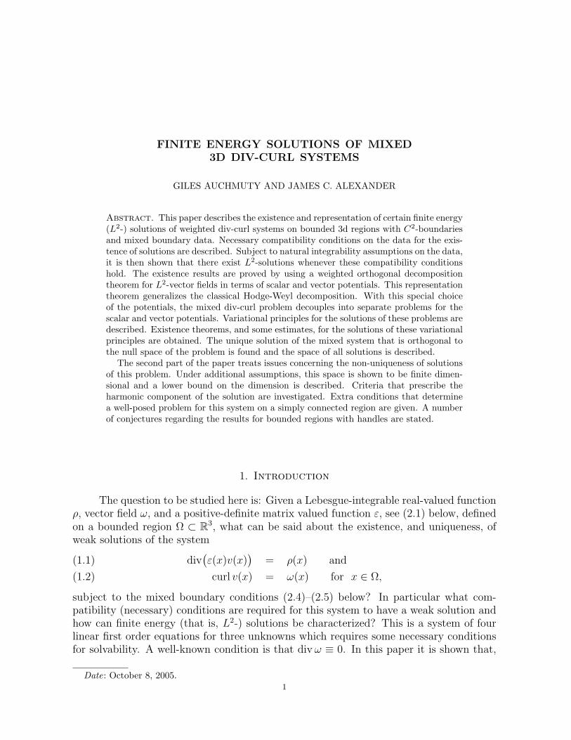
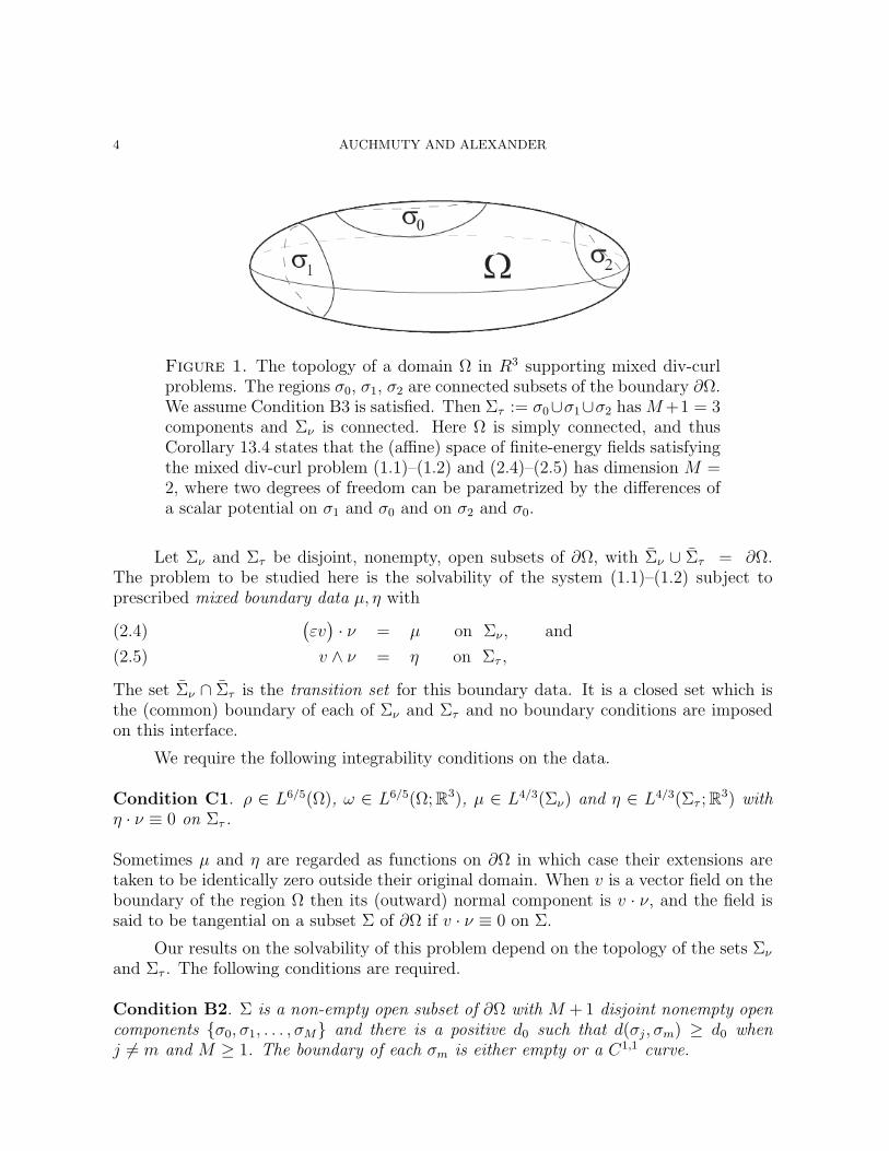
Figure 1. The topology of a domain Ω in R3 supporting mixed div-curlproblems. The regions σ0, σ1, σ2 are connected subsets of the boundary ∂Ω.We assume Condition B3 is satisfied. Then Στ := σ0∪σ1∪σ2 has M+1 = 3components and Σν is connected. Here Ω is simply connected, and thusCorollary 13.4 states that the (affine) space of finite-energy fields satisfyingthe mixed div-curl problem (1.1)–(1.2) and (2.4)–(2.5) has dimension M =2, where two degrees of freedom can be parametrized by the differences ofa scalar potential on σ1 and σ0 and on σ2 and σ0.

Let Σν and Στ be disjoint, nonempty, open subsets of ∂Ω, with Σν ∪ Στ = ∂Ω.The problem to be studied here is the solvability of the system (1.1)–(1.2) subject toprescribed mixed boundary data µ, η with(

εv)· ν = µ on Σν , and(2.4)

v ∧ ν = η on Στ ,(2.5)

The set Σν ∩ Στ is the transition set for this boundary data. It is a closed set which isthe (common) boundary of each of Σν and Στ and no boundary conditions are imposedon this interface.

We require the following integrability conditions on the data.

Condition C1. ρ ∈ L6/5(Ω), ω ∈ L6/5(Ω; R3), µ ∈ L4/3(Σν) and η ∈ L4/3(Στ ; R3) withη · ν ≡ 0 on Στ .

Sometimes µ and η are regarded as functions on ∂Ω in which case their extensions aretaken to be identically zero outside their original domain. When v is a vector field on theboundary of the region Ω then its (outward) normal component is v · ν, and the field issaid to be tangential on a subset Σ of ∂Ω if v · ν ≡ 0 on Σ.

Our results on the solvability of this problem depend on the topology of the sets Σν

and Στ . The following conditions are required.

Condition B2. Σ is a non-empty open subset of ∂Ω with M + 1 disjoint nonempty opencomponents σ0, σ1, . . . , σM and there is a positive d0 such that d(σj, σm) ≥ d0 whenj 6= m and M ≥ 1. The boundary of each σm is either empty or a C1,1 curve.


ΩΣ

Σ

Σ

Σσ σ1

2

3

0

0 1

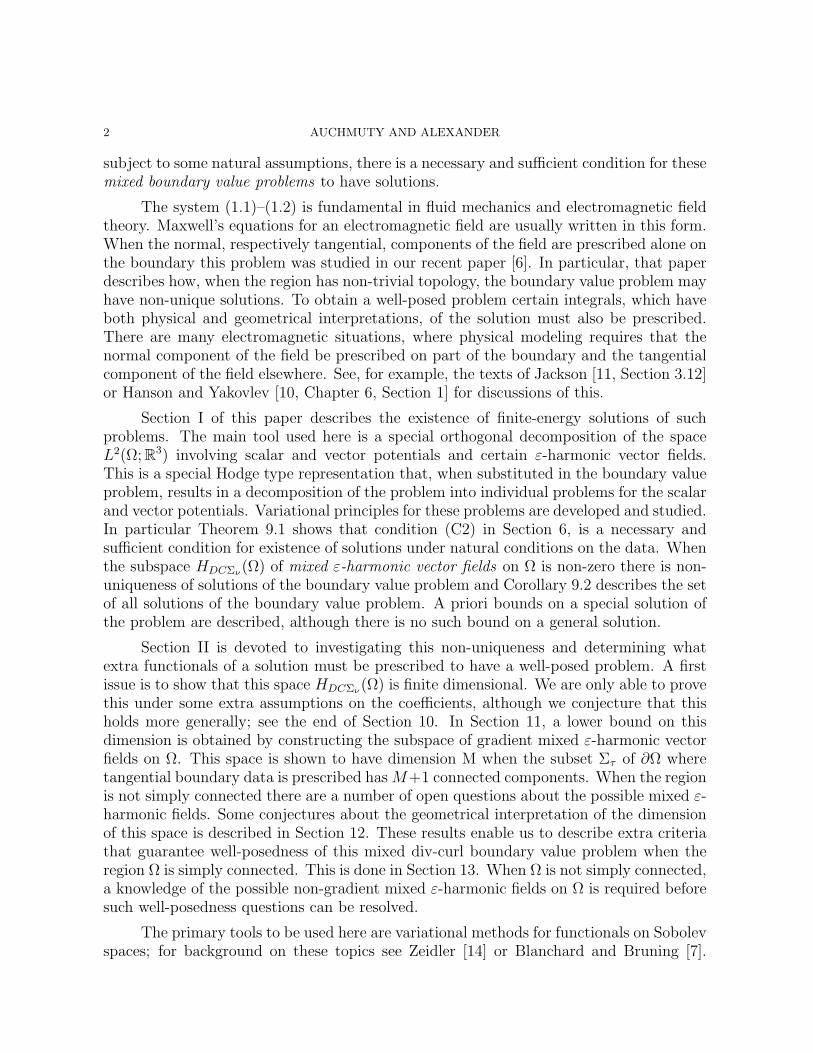
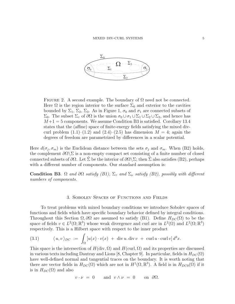
Figure 2. A second example. The boundary of Ω need not be connected.Here Ω is the region interior to the surface Σ0 and exterior to the cavitiesbounded by Σ1, Σ2, Σ3. As in Figure 1, σ0 and σ1 are connected subsets ofΣ0. The subset Στ of ∂Ω is the union σ0 ∪σ1 ∪Σ1 ∪Σ2 ∪Σ3, and hence hasM+1 = 5 components. We assume Condition B3 is satisfied. Corollary 13.4states that the (affine) space of finite-energy fields satisfying the mixed div-curl problem (1.1)–(1.2) and (2.4)–(2.5) has dimension M = 4; again thedegrees of freedom are parametrized by differences in a scalar potential.

Here d(σj, σm) is the Euclidean distance between the sets σj and σm. When (B2) holds,the complement ∂Ω\Σ is a non-empty compact set consisting of a finite number of closedconnected subsets of ∂Ω. Let Σ be the interior of ∂Ω\Σ; then Σ also satisfies (B2), perhapswith a different number of components. Our standard assumption is:

Condition B3. Ω and ∂Ω satisfy (B1), Στ and Σν satisfy (B2), possibly with differentnumbers of components.

3. Sobolev Spaces of Functions and Fields

To treat problems with mixed boundary conditions we introduce Sobolev spaces offunctions and fields which have specific boundary behavior defined by integral conditions.Throughout this Section Ω, ∂Ω are assumed to satisfy (B1). Define HDC(Ω) to be thespace of fields v ∈ L2(Ω; R3) whose weak divergence and curl are in L2(Ω) and L2(Ω; R3)respectively. This is a Hilbert space with respect to the inner product

(3.1) 〈u, v 〉DC :=

∫Ω

[u(x) · v(x) + div u. div v + curlu · curl v] d3x.

This space is the intersection of H(div,Ω) and H(curl,Ω) and its properties are discussedin various texts including Dautray and Lions [8, Chapter 9]. In particular, fields inHDC(Ω)have well-defined normal and tangential traces on the boundary. It is worth noting thatthere are vector fields in HDC(Ω) which are not in H1(Ω,R3). A field is in HDC0(Ω) if itis in HDC(Ω) and also

v · ν = 0 and v ∧ ν = 0 on ∂Ω.


To incorporate the boundary conditions we assume Σ is a nonempty open subset of∂Ω which satisfies (B2) and Σ := ∂Ω\Σ is also a non-empty open subset of ∂Ω. For suchΣ, let H1

Σ0(Ω) be the space of all functions ϕ ∈ H1(Ω), whose trace on Σ is zero. Define

(3.2) GΣ(Ω) := ∇ϕ : ϕ ∈ H1Σ0(Ω).

When v ∈ HDC(Ω), we say that v · ν = 0 weakly on Σ provided

(3.3)

∫Ω

[ v · ∇ϕ + ϕ div v ] d3x = 0 for all ϕ ∈ H1Σ0(Ω).

Let C1Σ0(Ω : R3) be the space of continuously differentiable vector fields on Ω which also

are continuous on Ω and satisfy

(3.4) v · ν = 0 on Σ and v ∧ ν = 0 on Σ.

We say that v ∧ ν = 0 weakly on Σ provided

(3.5)

∫Ω

[u · curl v − v · curlu ] d3x = 0 for all u ∈ C1Σ0(Ω : R3).

When v is continuous on Ω, continuously differentiable on Ω and in HDC(Ω) then thesedefinitions agree with the classical definitions as a consequence of the Gauss-Green The-orem.

Let HDCΣ(Ω) denote be the closure of the space C1Σ0(Ω : R3) with respect to the DC-

inner product (3.1). Such fields are in HDC(Ω) and satisfy the null boundary conditions(3.4) in the weak sense defined above. Many properties of this space were proved inAuchmuty [3] and a number of results from that paper are used here.

Lemma 3.1. Assume (B1) holds and Σ is a non-empty open subset of ∂Ω; then H1Σ0(Ω)

is a closed subspace of H1(Ω). If ∇ϕ ∈ GΣ(Ω), then ∇ϕ ∧ ν = 0 weakly on Σ.

Proof. Let ϕn : n ≥ 1 be a sequence of functions in H1Σ0(Ω) which converge to a limit

ϕ in H1(Ω). Then ϕn → ϕ ∈ L2(∂Ω, dσ) from [9, Section 4.3, Theorem 1]. Moreover,∫∂Ωϕnψ dσ = 0 for all ψ which are continuous on ∂Ω and have compact support in

Σ since the trace of each ϕn = 0 on Σ. Let n increase to ∞ then, by continuity, thesame is true for ϕ, and the subspace is closed. Suppose now that ϕ is C1 on Ω then theGauss-Green Theorem yields that∫

Ω

∇ϕ · curlA d3x =

∫Σ

A · (∇ϕ ∧ ν) dσ +

∫Σ

A · (∇ϕ ∧ ν) dσ.(3.6)

=

∫Σ

A · (∇ϕ ∧ ν) dσ for all A ∈ C1Σ0(Ω : R3).(3.7)

When ϕ and ∂Ω are smooth the first term on the right hand side is zero from classicalcalculus so the left hand side is zero. By density this then holds for all ϕ ∈ H1

Σ0(Ω), sothe second sentence of the lemma follows upon substituting ∇ϕ for v in (3.5).

Define the space

(3.8) CurlεΣ(Ω) := ε−1 curlA : A ∈ HDCΣ(Ω).


An essential result about this space is the following

Lemma 3.2. Suppose Σ, ∂Ω satisfy (B1); then CurlεΣ(Ω) is a subspace of L2(Ω; R3) thatis ε-orthogonal to GΣ(Ω). Moreover curl A · ν ∈ H−1/2(∂Ω) and curl A · ν = 0 weakly onΣ.

Proof. When ε satisfies condition (E1), so does ε−1 and thus ε−1 curlA ∈ L2(Ω; R3)as curlA ∈ L2(Ω; R3) whenever A ∈ HDCΣ(Ω). Suppose w := ∇ϕ ∈ GΣ(Ω) and v :=ε−1 curlA ∈ CurlεΣ(Ω); then

〈 v, w 〉ε =

∫Ω

∇ϕ · curlA d3x.

When A ∈ C1Σ0(Ω : R3), then (3.6) holds as above, so 〈 v, w 〉ε = 0 from Lemma 3.1

and the boundary condition on A. For general A ∈ HDCΣ(Ω), let A(m) : m ≥ 1 be asequence of fields in C1

Σ0(Ω : R3) which converge to A in the DC-norm. For each m ≥ 1,

we have 〈w, ε−1 curlA(m) 〉ε = 0, so taking limits one finds 〈 v, w 〉ε = 0 again and the

spaces are ε-orthogonal as claimed. For any ϕ ∈ H1(Ω) and a smooth field A on Ω, thedivergence theorem yields

(3.9)

∫Ω

∇ϕ · curlA d3x =

∫∂Ω

ϕ (curlA · ν) dσ.

When A ∈ HDC(Ω), this and the H1-trace theorem imply that curl A · ν ∈ H−1/2(∂Ω) asthe left hand side is continuous. When ϕ ∈ H1

Σ0(Ω) and A ∈ HDCΣ(Ω), this integral is

zero from the first part of the lemma, so curl A ·ν = 0 on Σ as (3.3) holds with v replacedby curlA.

Lemma 3.3. Suppose Σ, ∂Ω satisfy (B1). A field v ∈ HDC(Ω) is ε-orthogonal to GΣ(Ω)if and only if, in a weak sense,

(3.10) div(εv) = 0 on Ω and (εv) · ν = 0 on Σ.

It is ε-orthogonal to CurlεΣ(Ω) if and only if, in a weak sense,

(3.11) curl v = 0 on Ω and v ∧ ν = 0 on Σ.

Proof. When v is ε-orthogonal to GΣ(Ω) use of the Gauss-Green Theorem yields∫∂Ω

ϕ((εv) · ν) dσ −∫

Ω

ϕ div(εv) d3x = 0 for all ϕ ∈ H1Σ0(Ω).

This is the weak form of (3.10) from (3.3). When A ∈ HDCΣ(Ω), v ∈ HDC(Ω) then, fromGauss-Green,

〈 v, ε−1 curlA 〉ε =

∫Ω

v · curlA d3x =

∫∂Ω

A · (v ∧ ν) dσ +

∫Ω

A · curl v d3x.

This surface integral may be written∫∂Ω

A · (v ∧ ν) dσ =

∫Σ

A · (v ∧ ν) dσ +

∫Σ

v · (ν ∧ A) dσ.


When v is ε-orthogonal to CurlεΣ(Ω), this yields

(3.12) 0 =

∫Σ

A · (v ∧ ν) dσ +

∫Ω

A · curl v d3x for all A ∈ HDCΣ(Ω).

This is the weak form of (3.11) and the result follows.

Lemma 3.2 states thatGΣ(Ω) and CurlεΣ(Ω) are ε-orthogonal subspaces of L2(Ω; R3);in general they do not span L2(Ω; R3). Define HεΣ(Ω) to be the class of all vector fields inL2(Ω; R3) which are ε-orthogonal to CurlεΣ(Ω) and also to GΣ(Ω). This definition guar-antees that HεΣ(Ω) is a closed subspace of L2(Ω; R3) and may be characterized explicitlyas follows.

Lemma 3.4. A vector field h ∈ L2(Ω; R3) ∈ HεΣ(Ω) if and only if it satisfies∫Ω

(εh) · ∇ϕ d3x = 0 for all ϕ ∈ H1Σ0(Ω), and(3.13) ∫

Ω

h · curlA d3x = 0 for all A ∈ HDCΣ(Ω).(3.14)

Proof. This is just a matter of rewriting the two ε-orthogonality conditions.

In particular this states that a field is in HεΣ(Ω) if and only if it is a weak solutionof (3.10) and (3.11). That is, the fields satisfy the boundary conditions

(3.15) (εh) · ν = 0 on Σ and h ∧ ν = 0 on Σ

in a weak sense.

A vector field h ∈ L2(Ω; R3) is defined to be ε-harmonic on Ω provided it satisfiesthe system ∫

Ω

(εh) · ∇ϕ d3x = 0 for all ϕ ∈ H10 (Ω), and(3.16) ∫

Ω

h · curlA d3x = 0 for all A ∈ HDC0(Ω).(3.17)

Fields in HεΣ(Ω) are called mixed ε-harmonic fields since they satisfy mixed boundary

conditions and are harmonic on Ω. When ε ≡ I3, such fields are called mixed (or Σ-)harmonic fields and the corresponding spaces are denoted HΣ(Ω). Substituting Σ for Σ,this convention shows that HΣ(Ω) ⊂ HDCΣ(Ω).


I. SOLVABILITY of MIXED DIV-CURL SYSTEMS.

4. Mixed Weighted Orthogonal Decompositions

Our approach to studying the solvability of this mixed div-curl system is modeled onthe method used in [6] for the cases of given normal, respectively tangential, componentsof the field. Namely we describe certain classes of scalar and vector potentials that providean ε-orthogonal decomposition of finite energy (or L2) fields of the form

(4.1) v(x) = ∇ϕ(x) + ε(x)−1 curlA(x) + h(x).

Here h is an ε-harmonic vector field on Ω. Throughout this Section, we use the ε- innerproduct on L2(Ω; R3). The representation result to be used here is the following general-ization of the classical Hodge-Weyl decomposition. The usual Hodge-Weyl decompositiondescribed in [2], [8, Chapter 9], or [6] and elsewhere corresponds to the case ε(x) ≡ I3and the choices Στ = ∅ or ∂Ω in the following analysis.

Theorem 4.1. Assume (B3) and (E1) hold; then

(4.2) L2(Ω; R3) = GΣτ (Ω)⊕ε CurlεΣτ (Ω)⊕ε HεΣν (Ω),

with GΣτ (Ω), CurlεΣτ (Ω) and HεΣν (Ω) defined as in Section 3.

Proof. The definitions (3.2) and (3.8) show that these spaces are subspaces of L2(Ω; R3).They are orthogonal from Lemma 3.2 and the definition of HεΣν (Ω). Thus the theoremis proved provided we can show that each of the spaces is closed. This is done below inTheorems 4.2 and 5.2 respectively.

This result states that the scalar potential ϕ in (4.1) may be chosen to be inH1Στ0(Ω).

When the vector potential A ∈ HDCΣτ (Ω), the corresponding class of vector fields is ε-orthogonal from Lemma 3.2. The space HεΣν (Ω) appearing here is the null space of ourproblem (1.1)–(1.2) and (2.4)–(2.5). Fields in HεΣν (Ω) are ε-harmonic fields that satisfy(3.15) in a weak sense with Στ in place of Σ.

Given v ∈ L2(Ω; R3), Riesz’ Theorem states that the projection of v onto GΣτ (Ω) isgiven by PG(v) = ∇ϕv where ϕv minimizes ‖v−∇ϕ‖ε over all ϕ ∈ GΣτ (Ω). Equivalentlyϕv minimizes Dv : H1

Στ0(Ω) → R defined by

(4.3) Dv(ϕ) :=

∫Ω

[(ε∇ϕ) · ∇ϕ− 2(εv) · ∇ϕ] d3x.

The existence-uniqueness result for this variational problem may be stated as follows.

Theorem 4.2. Assume (B3) and (E1) hold and v ∈ L2(Ω; R3). Then there is a uniqueϕv which minimizes Dv on H1

Στ0(Ω). A function ϕv minimizes Dv on H1Στ0(Ω) if and only

if it satisfies

(4.4)

∫Ω

[ε(∇ϕ− v)] · ∇ψ d3x = 0 for all ψ ∈ H1Στ0(Ω).


GΣτ (Ω) is a closed subspace of L2(Ω; R3) and the projection PG of L2(Ω; R3) onto GΣτ (Ω)is given by PGv := ∇ϕv.

Proof. The functional Dv is continuous and convex from standard arguments, so it isweakly lower semi-continuous on H1

Στ0(Ω). Theorem 5.1 of [3] states that there is aλ1 > 0 such that∫

Ω

|∇ϕ|2 d3x ≥ λ1

∫Ω

|ϕ|2 d3x for all ϕ ∈ H1Στ0(Ω).

Substitute this, the Schwarz inequality and (2.1) in (4.3); then

2Dv(ϕ) ≥[∫

Ω

e0|∇ϕ|2 d3x + λ1

∫Ω

|ϕ|2 d3x

]− 4 ‖εv‖2 ‖∇ϕ‖2 .

Thus Dv is coercive and strictly convex so it has a unique minimizer ϕv on H1Στ0(Ω).

Straightforward analysis shows that the Gateaux derivative of Dv is given by

〈D′v(ϕ), ψ 〉 = 2

∫Ω

[ε(∇ϕ− v)] · ∇ψ d3x for ϕ, ψ ∈ H1Στ0(Ω).

Thus ϕv is a minimizer of Dv on H1Στ0(Ω) if and only if (4.4) holds. Since this variational

problem has a solution for each v ∈ L2(Ω; R3), [2, Corollary 3.3] yields the last sentenceof the theorem.

When ϕv, ε are sufficiently smooth applying the Gauss-Green Theorem to the inte-gral in (4.4), yields∫

∂Ω

ψ[ε(∇ϕv − u)] · ν dσ +

∫Ω

ψ∇(ε(∇ϕ− v)) d3x = 0 for all ψ ∈ H1Στ0(Ω).

Thus (4.4) may be regarded as a weak form of the system

(4.5) div(ε∇ϕ) = div(εv) on Ω, subject to

(4.6) ϕ ≡ 0 on Στ and(ε(∇ϕ)

)· ν = (εv) · ν on Σν .

This type of elliptic mixed boundary value problem has been extensively studied. SeeStephan [12] for a treatment of such problems in three dimensional cases using boundaryintegral methods.

5. The Mixed Vector Potential

The vector field A in the representation (4.1) is called a weighted vector potential ofv associated with ε. When ε ≡ I3, such fields are just called vector potentials for v. Forgiven v there is a large class of such (weighted) vector potentials. The analysis of ourproblems is simplified by a special choice of this vector potential. The following is a slightmodification of [3, Proposition 7.2].


Theorem 5.1. Suppose Στ , ∂Ω satisfy (B3) and A ∈ HDCΣτ (Ω). Then there is a unique

A ∈ HDCΣτ (Ω) such that

(1) div A = 0, and curl A = curlA on Ω, and

(2) A is L2-orthogonal to HΣτ (Ω).

Proof. Given such an A, let ϕ ∈ H1Σν0(Ω) be the unique minimizer of

DA(ϕ) :=

∫Ω

(|∇ϕ|2 − 2A · ∇ϕ) d3x

on H1Σν0(Ω). This problem may be analyzed just as in Theorem 4.2 and ϕ is a weak

solution of the system

(5.1) ∆ϕ = divA on Ω, subject to

(5.2) ϕ ≡ 0 on Σν and ∇ϕ · ν = 0 on Στ .

This follows similar to equations (4.5)-(4.6) above. The vector field A := A − ∇ϕ ∈HDCΣτ (Ω) and satisfies

(5.3) div A = 0 and curl A = curlA on Ω.

If HΣτ (Ω) = 0, the result follows. When HΣτ (Ω) is non-zero, let PH be the orthogonal

projection of HDCΣτ (Ω) onto this closed subspace. Then A := (I − PH)A has properties

(1) and (2). If B is another vector field which satisfies these conditions, then A−B is in

HΣτ (Ω). From property (ii) it is also L2-orthogonal to HΣτ (Ω), so A = B.

Define ZΣτ (Ω) to be the subspace of fields A ∈ HDCΣτ (Ω) that also satisfy

(5.4) divA = 0 on Ω and are L2-orthogonal to HΣτ (Ω).

These conditions imply that ZΣτ (Ω) is a closed subspace of HDCΣτ (Ω). Define QC to bethe orthogonal projection of HDCΣτ (Ω) onto ZΣτ (Ω). Thus Theorem 5.1 implies that (3.8)can be written as

(5.5) CurlεΣτ (Ω) = ε−1 curlA : A ∈ ZΣτ (Ω);i.e., fields in CurlεΣτ (Ω) have a unique vector potential in ZΣτ (Ω). Moreover by reviewingthe construction in this theorem, one sees that each field A ∈ HDCΣτ (Ω) has a represen-tation

(5.6) A = QCA + ∇ϕ + k, with ϕ ∈ H1Σν0(Ω) and k ∈ HΣτ (Ω).

Let PC be the ε-orthogonal projection of L2(Ω; R3) onto the closure of CurlεΣτ (Ω).To complete the proof of Theorem 4.1 and show that CurlεΣτ (Ω) is a closed subspace ofL2(Ω; R3), we study the associated projection. Given v ∈ L2(Ω; R3), Riesz’ Theorem forprojections states that PCv := curlAv where Av minimizes ‖v− ε−1 curlA‖ε on ZΣτ (Ω).That is Av minimizes

(5.7) Cv(A) :=

∫Ω

[(ε−1 curlA) · curlA− 2v · curlA] d3x


on ZΣτ (Ω). The existence of solutions of this variational problem may be described asfollows.

Theorem 5.2. Assume (B3) and (E1) hold and v ∈ L2(Ω; R3). Then there is a uniqueAv which minimizes Cv on ZΣτ (Ω). A field A minimizes Cv on HDCΣτ (Ω) if and only if itsatisfies

(5.8)

∫Ω

(ε−1 curlA− v) · curlB d3x = 0 for all B ∈ HDCΣτ (Ω).

Moreover CurlεΣτ (Ω) is a closed subspace of L2(Ω; R3) and the projection PC of L2(Ω; R3)onto CurlεΣτ (Ω) is given by PCv := curlA where A is any minimizer of Cv on HDCΣτ (Ω).

Proof. The functional Cv is convex and continuous on ZΣτ (Ω), so it is weakly l.s.c. From[3, equation (8.18)] there is a µ1 > 0 such that∫

Ω

| curlA|2 d3x ≥ µ1

∫Ω

|A|2 d3x for all A ∈ ZΣτ (Ω).

This, Schwarz inequality and (2.1) applied to (5.7) yield

Cv(A) ≥ (2e1)−1

∫Ω

[| curlA|2 + µ1|A|2

]d3x − 2 ‖v‖2 ‖curlA‖2

Thus Cv is coercive and strictly convex on ZΣτ (Ω) so it has a unique minimizer Av onZΣτ (Ω). The extremality condition (5.8) holds for all B ∈ ZΣτ (Ω) upon evaluation ofthe Gateaux derivative of the functional Cv. Note that this functional may be extendedto HDCΣτ (Ω) with the same formulae and the same minimal value, so (5.8) holds forall B ∈ HDCΣτ (Ω) and any minimizer in HDCΣτ (Ω). Since this variational problemhas a solution for each v ∈ L2(Ω; R3), [2, Corollary 3.3] yields the last sentence of thetheorem.

6. Necessary Conditions for Solvability

The div-curl boundary value problem (1.1)–(1.2) with (2.4)–(2.5) cannot have a so-lution for arbitrary fields ω, η. An obvious further condition is that ω should be solenoidal.In fact the following stronger criterion must hold.

Theorem 6.1. (Necessary conditions) Assume (B2) and (C1) hold and v ∈ L2(Ω; R3)is a weak solution of (1.1), (1.2) and (2.4)–(2.5). Then the data must satisfy condition[C2]:

(6.1)

∫Ω

ω ·Ad3x +

∫Στ

η ·A dσ = 0 for any irrotational field A ∈ HDCΣτ (Ω).

Proof. Multiply (1.2) by A ∈ HDCΣτ (Ω) and integrate. Then the definition of A yields∫Ω

ω · Ad3x =

∫Στ

v · (A ∧ ν) dσ +

∫Ω

v · curlAd3x.


When A is irrotational then (C2) follows upon using (2.5) and the fact that η · ν = 0 on∂Ω.

A field A ∈ HDCΣτ (Ω) is irrotational on Ω if and only if it has the form

(6.2) A = h + ∇ϕ where ϕ ∈ H1Σν0(Ω) and h ∈ HΣτ (Ω)

from Auchmuty [3, Theorem 7.2]. Substitute ∇ϕ for A in (C2) to find

(6.3)

∫Στ

[ϕ(ω · ν) + η · ∇ϕ] dσ −∫

Ω

ϕ divω d3x = 0 for all ϕ ∈ H1Σν0(Ω).

This implies that ω must be solenoidal on Ω and also that a weak form of a continuityequation holds on Στ . Namely

(6.4)

∫Στ

[ϕ(ω · ν) + η · ∇ϕ] dσ = 0 for all ϕ ∈ H1Σν0(Ω).

This equation relates ω and η on each component of Στ and may be interpreted as aversion of Kirchoff’s law for currents. The condition (C2) also require the compatibilityconditions

(6.5)

∫Ω

ω · h d3x +

∫Στ

η · h dσ = 0 for h ∈ HΣτ (Ω)

The number of independent conditions here is equal to the dimension of HΣτ (Ω).

7. Variational Principles for the Scalar Potentials

When the potentials in the representation (4.1) are chosen as in Theorem 4.1, theequations for the scalar and vector potentials decouple. The equations for the scalarpotential become

(7.1) div(ε(x)∇ϕ(x)

)= ρ(x) on Ω,

(7.2)(ε(x)∇ϕ(x)

)· ν(x) = µ(x) on Σν and ϕ(x) = 0 on Στ .

A weak form of this equation is to find ϕ ∈ H1Στ0(Ω) satisfying

(7.3)

∫Ω

[(ε∇ϕ) · ∇X + ρX ] d3x −∫

Σν

µX dσ = 0 for all X ∈ H1Στ0(Ω).

The solution of this equation may be characterized as the minimizer of a natural varia-tional principle. Consider the problem of minimizing D : H1

Στ0(Ω) → R defined by

(7.4) D(ϕ) :=

∫Ω

[(ε(∇ϕ) · ∇ϕ

)+ 2ρϕ

]d3x −

∫Σν

2µϕ dσ.

The existence and uniqueness result for this problem is the following

Theorem 7.1. Assume (B3), (C1) and (E1) hold. Then D is bounded below on H1Στ0(Ω)

and has a unique minimizer ϕ. This minimizer is the unique weak solution of (7.3).


Proof. When Στ obeys (B2), H1Στ0(Ω) is a closed subspace of H1(Ω) from Lemma 3.1. The

proof that D is a continuous convex functional is standard. Theorem 5.1 of [3] providesa coercivity inequality of the form

(7.5)

∫Ω

|∇ϕ|2 d3x ≥ λ1

∫Ω

|ϕ|2 d3x for all ϕ ∈ H1Στ0(Ω).

Since (E1) holds, we find that D is strictly convex and coercive on H1Στ0(Ω), so it is

bounded below and attains a unique minimizer on this space. The quadratic functionalD is Gateaux differentiable. Thus a function minimizes D on H1

Στ0(Ω) if and only if andit satisfies (7.3) from a standard result for convex minimization.

As is usual in quadratic variational problems, the continuous dependence of thesolutions on the data is quantified by bounds on the solutions. For this problem we havethe following.

Theorem 7.2. Assume (B3), (C1) and (E1) hold and ϕ is the unique solution of (7.3)in H1

Στ0(Ω) . Then there are constants C1, C2 such that

(7.6) ‖∇ϕ‖2 ≤ C1‖ρ‖6/5,Ω + C2‖µ‖4/3,Σν .

Proof. The regularity condition (B1) is sufficient to ensure that the Sobolev imbeddingtheorem and the trace theorem holds for functions in H1(Ω). Moreover ‖∇ϕ‖2 defines anorm on H1

Στ0(Ω) that is equivalent to the usual H1-norm since (7.5) holds. Thus thereare constants b1, b2 which depend only on Ω, ∂Ω such that

(7.7) ‖ϕ‖6,Ω ≤ b1‖∇ϕ‖2 and ‖ϕ‖4,∂Ω ≤ b2‖∇ϕ‖2.

Use this, (2.1) and Holder’s inequality in (7.4); then

D(ϕ) ≥ e0‖∇ϕ‖22 − 2

[b1‖ρ‖6/5,Ω + b2‖µ‖4/3,Σν

]‖∇ϕ‖2.

The value of this variational problem cannot be positive, so the minimizer satisfies aninequality of the form (7.6).

8. Variational Principles for the Vector Potentials

Just as above, substitution of (4.1) in (1.1)–(1.2) and (2.4)–(2.5) leads to a systemof equations for the vector potential. They can be written

curl(ε(x)−1 curlA(x)

)= ω(x) on Ω,(8.1) (

ε−1(x) curlA(x))∧ ν(x) = η(x) on Στ , and(8.2)

A(x) ∧ ν(x) = 0 on Σν .(8.3)

A weak form of this system is to find A ∈ HDCΣτ (Ω) satisfying

(8.4)

∫Ω

[(ε−1 curlA) ·curlC−ω ·C] d3x −∫

Στ

η ·C dσ = 0 for all C ∈ HDCΣτ (Ω).


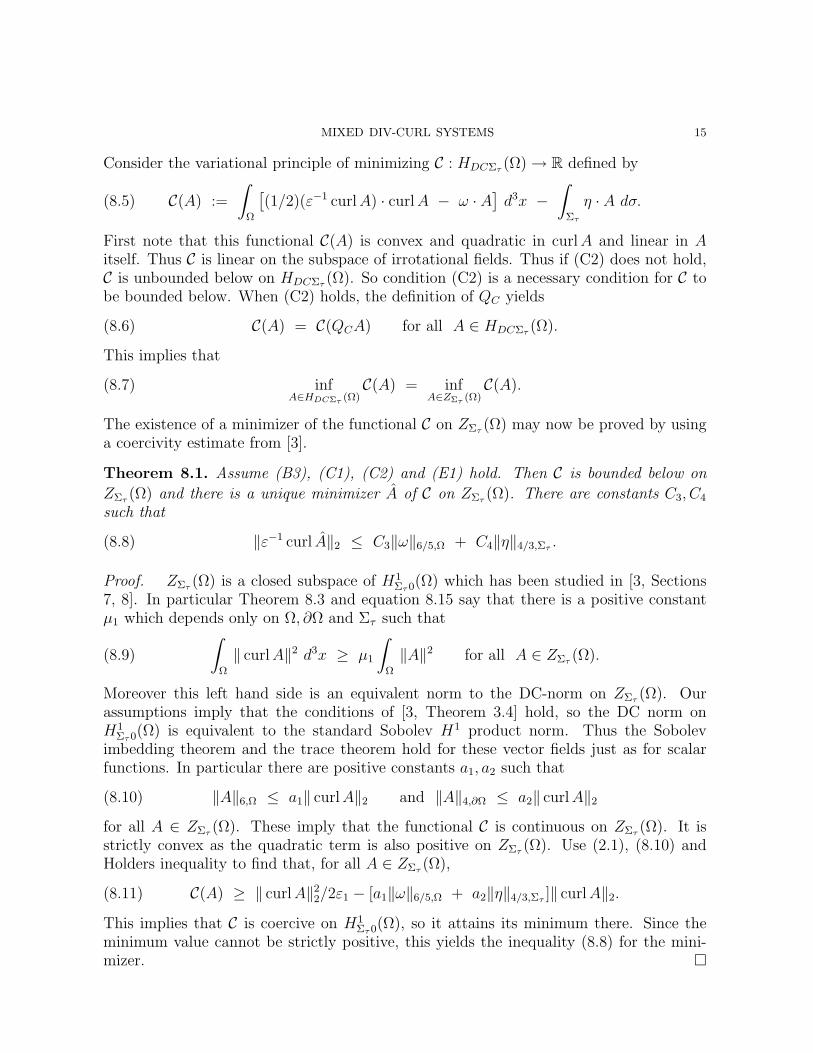
Consider the variational principle of minimizing C : HDCΣτ (Ω) → R defined by

(8.5) C(A) :=

∫Ω

[(1/2)(ε−1 curlA) · curlA − ω · A

]d3x −

∫Στ

η · A dσ.

First note that this functional C(A) is convex and quadratic in curlA and linear in Aitself. Thus C is linear on the subspace of irrotational fields. Thus if (C2) does not hold,C is unbounded below on HDCΣτ (Ω). So condition (C2) is a necessary condition for C tobe bounded below. When (C2) holds, the definition of QC yields

(8.6) C(A) = C(QCA) for all A ∈ HDCΣτ (Ω).

This implies that

(8.7) infA∈HDCΣτ (Ω)

C(A) = infA∈ZΣτ (Ω)

C(A).

The existence of a minimizer of the functional C on ZΣτ (Ω) may now be proved by usinga coercivity estimate from [3].

Theorem 8.1. Assume (B3), (C1), (C2) and (E1) hold. Then C is bounded below on

ZΣτ (Ω) and there is a unique minimizer A of C on ZΣτ (Ω). There are constants C3, C4

such that

(8.8) ‖ε−1 curl A‖2 ≤ C3‖ω‖6/5,Ω + C4‖η‖4/3,Στ .

Proof. ZΣτ (Ω) is a closed subspace of H1Στ0(Ω) which has been studied in [3, Sections

7, 8]. In particular Theorem 8.3 and equation 8.15 say that there is a positive constantµ1 which depends only on Ω, ∂Ω and Στ such that

(8.9)

∫Ω

‖ curlA‖2 d3x ≥ µ1

∫Ω

‖A‖2 for all A ∈ ZΣτ (Ω).

Moreover this left hand side is an equivalent norm to the DC-norm on ZΣτ (Ω). Ourassumptions imply that the conditions of [3, Theorem 3.4] hold, so the DC norm onH1

Στ0(Ω) is equivalent to the standard Sobolev H1 product norm. Thus the Sobolevimbedding theorem and the trace theorem hold for these vector fields just as for scalarfunctions. In particular there are positive constants a1, a2 such that

(8.10) ‖A‖6,Ω ≤ a1‖ curlA‖2 and ‖A‖4,∂Ω ≤ a2‖ curlA‖2

for all A ∈ ZΣτ (Ω). These imply that the functional C is continuous on ZΣτ (Ω). It isstrictly convex as the quadratic term is also positive on ZΣτ (Ω). Use (2.1), (8.10) andHolders inequality to find that, for all A ∈ ZΣτ (Ω),

(8.11) C(A) ≥ ‖ curlA‖22/2ε1 − [a1‖ω‖6/5,Ω + a2‖η‖4/3,Στ ]‖ curlA‖2.

This implies that C is coercive on H1Στ0(Ω), so it attains its minimum there. Since the

minimum value cannot be strictly positive, this yields the inequality (8.8) for the mini-mizer.


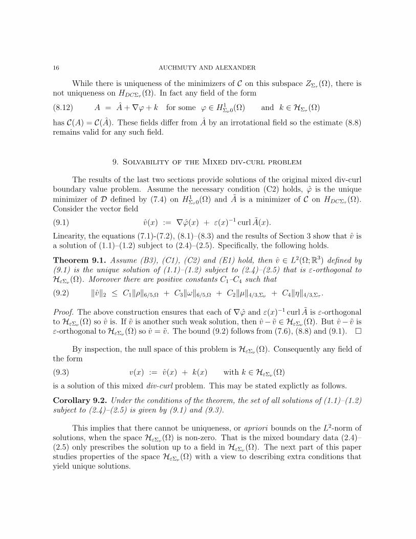
While there is uniqueness of the minimizers of C on this subspace ZΣτ (Ω), there isnot uniqueness on HDCΣτ (Ω). In fact any field of the form

(8.12) A = A+∇ϕ+ k for some ϕ ∈ H1Σν0(Ω) and k ∈ HΣτ (Ω)

has C(A) = C(A). These fields differ from A by an irrotational field so the estimate (8.8)remains valid for any such field.

9. Solvability of the Mixed div-curl problem

The results of the last two sections provide solutions of the original mixed div-curlboundary value problem. Assume the necessary condition (C2) holds, ϕ is the uniqueminimizer of D defined by (7.4) on H1

Στ0(Ω) and A is a minimizer of C on HDCΣτ (Ω).Consider the vector field

(9.1) v(x) := ∇ϕ(x) + ε(x)−1 curl A(x).

Linearity, the equations (7.1)-(7.2), (8.1)–(8.3) and the results of Section 3 show that v isa solution of (1.1)–(1.2) subject to (2.4)–(2.5). Specifically, the following holds.

Theorem 9.1. Assume (B3), (C1), (C2) and (E1) hold, then v ∈ L2(Ω; R3) defined by(9.1) is the unique solution of (1.1)–(1.2) subject to (2.4)–(2.5) that is ε-orthogonal toHεΣν (Ω). Moreover there are positive constants C1–C4 such that

(9.2) ‖v‖2 ≤ C1‖ρ‖6/5,Ω + C3‖ω‖6/5,Ω + C2‖µ‖4/3,Σν + C4‖η‖4/3,Στ .

Proof. The above construction ensures that each of ∇ϕ and ε(x)−1 curl A is ε-orthogonalto HεΣν (Ω) so v is. If v is another such weak solution, then v− v ∈ HεΣν (Ω). But v− v isε-orthogonal to HεΣν (Ω) so v = v. The bound (9.2) follows from (7.6), (8.8) and (9.1).

By inspection, the null space of this problem is HεΣν (Ω). Consequently any field ofthe form

(9.3) v(x) := v(x) + k(x) with k ∈ HεΣν (Ω)

is a solution of this mixed div-curl problem. This may be stated explictly as follows.

Corollary 9.2. Under the conditions of the theorem, the set of all solutions of (1.1)–(1.2)subject to (2.4)–(2.5) is given by (9.1) and (9.3).

This implies that there cannot be uniqueness, or apriori bounds on the L2-norm ofsolutions, when the space HεΣν (Ω) is non-zero. That is the mixed boundary data (2.4)–(2.5) only prescribes the solution up to a field in HεΣν (Ω). The next part of this paperstudies properties of the space HεΣν (Ω) with a view to describing extra conditions thatyield unique solutions.


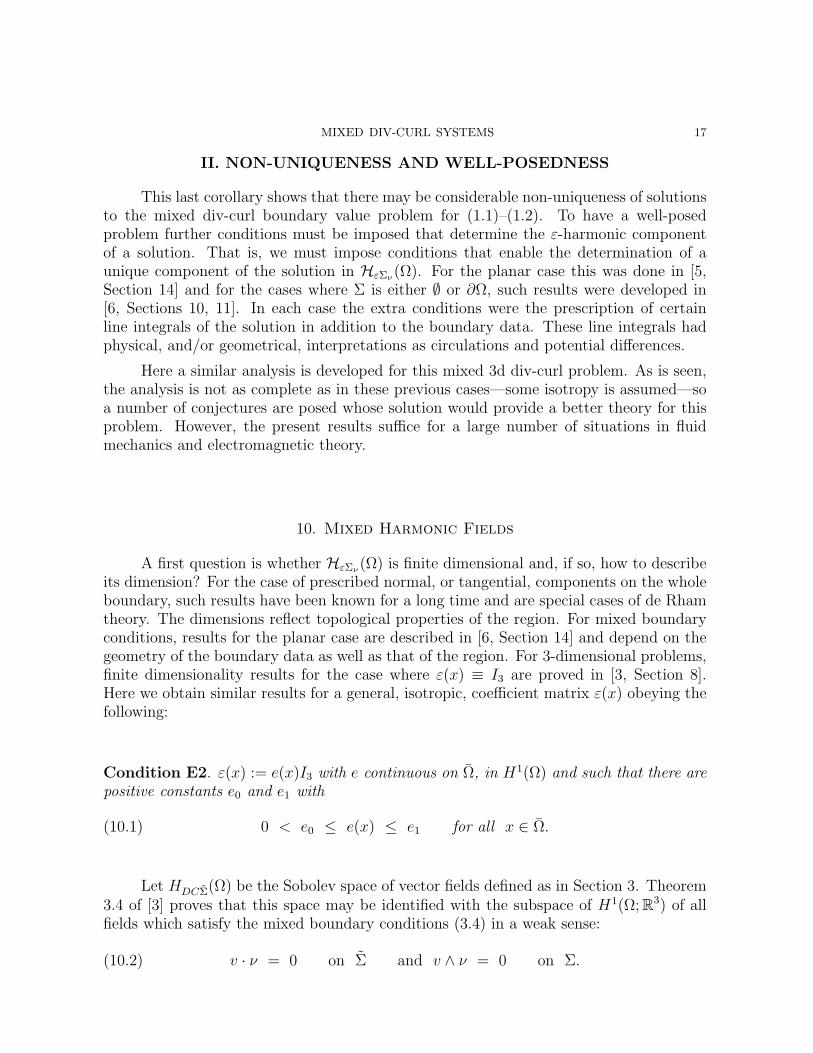
II. NON-UNIQUENESS AND WELL-POSEDNESS

This last corollary shows that there may be considerable non-uniqueness of solutionsto the mixed div-curl boundary value problem for (1.1)–(1.2). To have a well-posedproblem further conditions must be imposed that determine the ε-harmonic componentof a solution. That is, we must impose conditions that enable the determination of aunique component of the solution in HεΣν (Ω). For the planar case this was done in [5,Section 14] and for the cases where Σ is either ∅ or ∂Ω, such results were developed in[6, Sections 10, 11]. In each case the extra conditions were the prescription of certainline integrals of the solution in addition to the boundary data. These line integrals hadphysical, and/or geometrical, interpretations as circulations and potential differences.

Here a similar analysis is developed for this mixed 3d div-curl problem. As is seen,the analysis is not as complete as in these previous cases—some isotropy is assumed—soa number of conjectures are posed whose solution would provide a better theory for thisproblem. However, the present results suffice for a large number of situations in fluidmechanics and electromagnetic theory.

10. Mixed Harmonic Fields

A first question is whether HεΣν (Ω) is finite dimensional and, if so, how to describeits dimension? For the case of prescribed normal, or tangential, components on the wholeboundary, such results have been known for a long time and are special cases of de Rhamtheory. The dimensions reflect topological properties of the region. For mixed boundaryconditions, results for the planar case are described in [6, Section 14] and depend on thegeometry of the boundary data as well as that of the region. For 3-dimensional problems,finite dimensionality results for the case where ε(x) ≡ I3 are proved in [3, Section 8].Here we obtain similar results for a general, isotropic, coefficient matrix ε(x) obeying thefollowing:

Condition E2. ε(x) := e(x)I3 with e continuous on Ω, in H1(Ω) and such that there arepositive constants e0 and e1 with

(10.1) 0 < e0 ≤ e(x) ≤ e1 for all x ∈ Ω.

Let HDCΣ(Ω) be the Sobolev space of vector fields defined as in Section 3. Theorem3.4 of [3] proves that this space may be identified with the subspace of H1(Ω; R3) of allfields which satisfy the mixed boundary conditions (3.4) in a weak sense:

(10.2) v · ν = 0 on Σ and v ∧ ν = 0 on Σ.


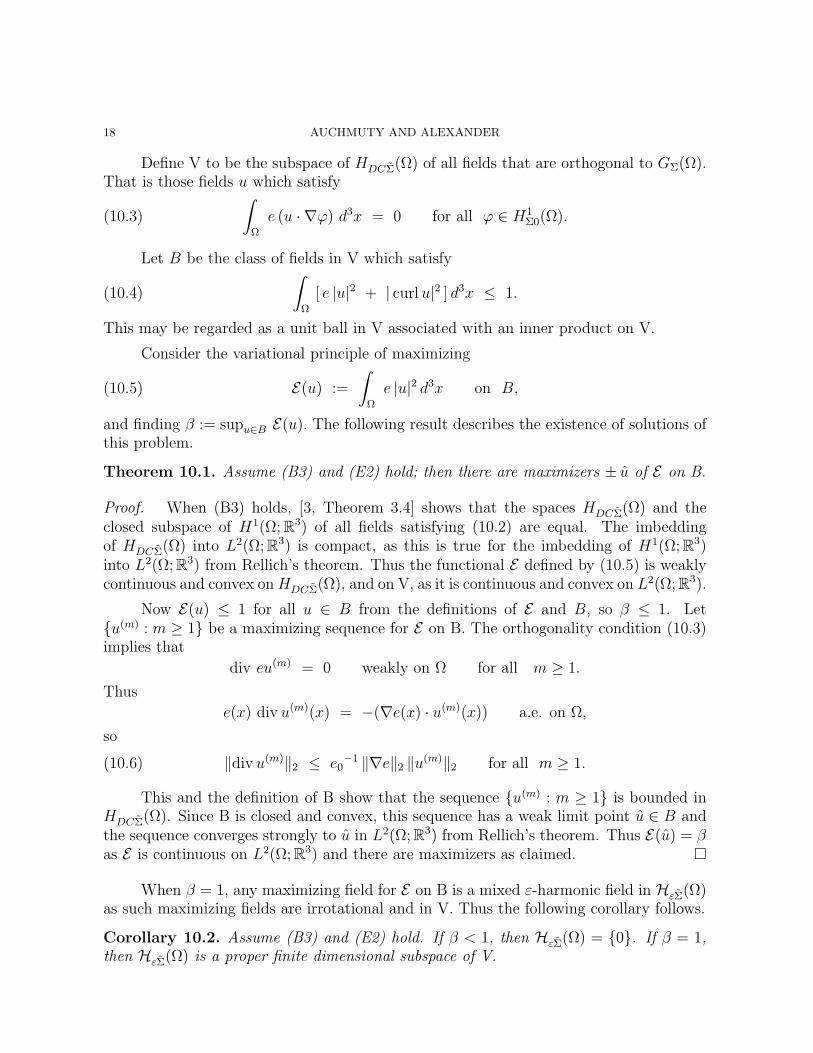
Define V to be the subspace of HDCΣ(Ω) of all fields that are orthogonal to GΣ(Ω).That is those fields u which satisfy

(10.3)

∫Ω

e (u · ∇ϕ) d3x = 0 for all ϕ ∈ H1Σ0(Ω).

Let B be the class of fields in V which satisfy

(10.4)

∫Ω

[ e |u|2 + | curlu|2 ] d3x ≤ 1.

This may be regarded as a unit ball in V associated with an inner product on V.

Consider the variational principle of maximizing

(10.5) E(u) :=

∫Ω

e |u|2 d3x on B,

and finding β := supu∈B E(u). The following result describes the existence of solutions ofthis problem.

Theorem 10.1. Assume (B3) and (E2) hold; then there are maximizers ± u of E on B.

Proof. When (B3) holds, [3, Theorem 3.4] shows that the spaces HDCΣ(Ω) and theclosed subspace of H1(Ω; R3) of all fields satisfying (10.2) are equal. The imbeddingof HDCΣ(Ω) into L2(Ω; R3) is compact, as this is true for the imbedding of H1(Ω; R3)into L2(Ω; R3) from Rellich’s theorem. Thus the functional E defined by (10.5) is weaklycontinuous and convex onHDCΣ(Ω), and on V, as it is continuous and convex on L2(Ω; R3).

Now E(u) ≤ 1 for all u ∈ B from the definitions of E and B, so β ≤ 1. Letu(m) : m ≥ 1 be a maximizing sequence for E on B. The orthogonality condition (10.3)implies that

div eu(m) = 0 weakly on Ω for all m ≥ 1.

Thus

e(x) div u(m)(x) = −(∇e(x) · u(m)(x)) a.e. on Ω,

so

(10.6) ‖div u(m)‖2 ≤ e0−1 ‖∇e‖2 ‖u(m)‖2 for all m ≥ 1.

This and the definition of B show that the sequence u(m) : m ≥ 1 is bounded inHDCΣ(Ω). Since B is closed and convex, this sequence has a weak limit point u ∈ B andthe sequence converges strongly to u in L2(Ω; R3) from Rellich’s theorem. Thus E(u) = βas E is continuous on L2(Ω; R3) and there are maximizers as claimed.

When β = 1, any maximizing field for E on B is a mixed ε-harmonic field in HεΣ(Ω)as such maximizing fields are irrotational and in V. Thus the following corollary follows.

Corollary 10.2. Assume (B3) and (E2) hold. If β < 1, then HεΣ(Ω) = 0. If β = 1,then HεΣ(Ω) is a proper finite dimensional subspace of V.


Proof. When β < 1, then v 6= 0 in B has curl v 6= 0, so HεΣ(Ω) = 0. Suppose β = 1then there is at least one mixed ε-harmonic field on Ω. Let F be a set of fields in HεΣ(Ω)which are orthonormal with respect to the inner product on V defined by

(10.7) 〈u, v 〉C :=

∫Ω

[ e u · v + curlu · curl v ] d3x

These fields are in B and are also orthonormal in L2(Ω; R3) as they are irrotational. Fcannot be infinite as B is compact in the weighted space L2(Ω; R3). Hence the subspaceHεΣ(Ω) must be finite dimensional.

This result shows that provided (B3) and (E2) holds, the corresponding space ofweighted harmonic fields is finite dimensional. It would be of interest to show thatdimHεΣ(Ω) is finite when we only require (B3) and (E1) to hold and we conjecturethat this is the case. A further conjecture is that this dimension is independent of thecoefficient matrix ε(x) provided (B3) and (E1) hold.

11. Gradient Mixed ε-Harmonic Fields.

In this section, a lower bound on the dimension ofHεΣ(Ω) is described which dependson the number of connected components of the set Σ where the tangential boundarycondition is imposed. Since the following analysis requires only that Condition (E1)holds, we treat this case. In Section 3, a field is defined to be in HεΣ(Ω) provided it isε-orthogonal to both GΣ(Ω) and CurlεΣ(Ω). That is, they satisfy (3.13)-(3.14) and, fromLemma 3.3, are weak solutions of the system

div (εh) = 0 and curlh = 0 on Ω,(11.1)

(εh) · ν = 0 on Σ and h ∧ ν = 0 on Σ.(11.2)

The gradient solutions of this system may be described explicitly. We show that, when Σhas M + 1 connected components, there are exactly M linearly independent such fields.Define GHεΣ(Ω) := G(Ω) ∩HεΣ(Ω) to be the subspace of gradient fields in HεΣ(Ω). Toconstruct a basis of GHεΣ(Ω) we need the following technical result.

Lemma 11.1. Assume ∂Ω satisfies (B1) and σ0, σ1 are disjoint open subsets of ∂Ω withσ0 connected and d(σ0, σ1) = d1 > 0. Then there is a C1 function g : ∂Ω → [0, 1] withg(x) = 1 on σ0 and g(x) = 0 on σ1.

Proof. When σ0, σ1 are subsets of different components of ∂Ω, take g to be identically1 or 0 on the different components and satisfy Laplace’s equation on Ω. The maximumprinciple, and regularity results, imply that g has the desired properties. When σ0, σ1

are subsets of the same component Σj of ∂Ω, take g to be identically 0 on the othercomponents. We construct the desired g on Σj. From Urysohn’s Lemma there is acontinuous function g0 on Σj with the desired properties. Introduce local coordinates onΣj and convolve g0 with a C1 mollifier of sufficiently small support. The resulting functionis the desired g.


With σ0, σ1 as in this lemma, define K(σ0, σ1) to be the subset of H1(Ω) of functionswhose trace is identically 1 on σ0 and 0 on σ1. This set has the following property.

Corollary 11.2. With ∂Ω, σ0, σ1 as above, K(σ0, σ1) is a closed convex subset of H1(Ω).

Proof. The C1 function constructed above has an extension to Ω from [13, Theorem8.8], and the extension is in K(σ0, σ1) . If u1, u2 are two functions in K(σ0, σ1), thenu1 − u2 ∈ H1

Σ0(Ω) where Σ = σ0 ∪ σ1. The result now follows from Lemma 3.1.

Assume that Σ := σ0, σ1, . . . , σM, M ≥ 1 has more than one component. Givenm with 0 ≤ m ≤ M , let χm be the minimizer of D0 defined by (4.3) with v ≡ 0 on theset Km := K(σm,Σ\σm). This problem has a unique minimizer as Km is a nonemptyclosed convex subset of H1(Ω). The minimizer satisfies

(11.3)

∫Ω

ε(∇χm) · ∇ϕ d3x = 0 for all ϕ ∈ H1Σ0(Ω).

This minimizing function χm is non-constant on Ω; so

(11.4) h(m)(x) := ∇χm(x).

is a non-zero field on Ω. Each h(m) ∈ HεΣ(Ω) as the functions χm are H1 solutions of thesystem (11.1) subject to

χ(x) =

1 for x ∈ σm,

0 for x ∈ Σ \ σm.(11.5)

together with the natural boundary conditions

(11.6)(ε(x)∇χ(x)

)· ν(x) = 0 on Σ.

The subspace GHεΣ(Ω) may now be characterized as follows.

Theorem 11.3. Assume ε satisfies (E1), (B1) holds and Σ has M + 1 components with

(B2) holding; then dimGHεΣ(Ω) = M . When M ≥ 1, then h(1), . . . , h(M) defined by(11.4) is a basis of GHεΣ(Ω).

Proof. Suppose h = ∇ψ ∈ GHεΣ(Ω) for some ψ in H1(Ω). From (3.13), it satisfies

(11.7)

∫Ω

(ε∇ψ) · ∇ϕ d3x = 0 for all ϕ ∈ H1Σ0(Ω).

Now the second part of the boundary condition (11.2) implies that ψ(x) ≡ cm isconstant on each component σm of Σ. When M = 0, then Σ = σ0 and ψ−c0 is in H1

Σ0(Ω).When Σ has positive surface measure, the uniqueness of solution of (11.7) implies thatψ ≡ c0, so GHεΣ(Ω) = 0. When M ≥ 1, we may choose c0 = 0 since the potential ψ isin H1(Ω). The definition of the χm then implies that

ψ(x) −M∑

m=1

cmχm(x) ≡ 0 on Σ.


Since ψ and each χm is a solution of (11.7), this right hand side is also a solution. It isidentically zero on Ω since it is zero on Σ . Take gradients then h is a linear combinationof h(1), . . . , h(M) so this set spans the subspace GHεΣ(Ω). These fields are independentfrom the boundary conditions on the χm so the theorem follows.

Suppose M ≥ 1 and h ∈ GHεΣ(Ω) with

(11.8) h(x) =M∑

m=1

cm h(m)(x),

The coefficients cm in this expansion can be determined using Fourier methods. Takeε-inner products of (11.8) with h(k); then

hk =M∑

m=1

hkm cm where hkm := 〈 h(k), h(m) 〉ε, and(11.9)

hk := 〈h, h(k) 〉ε =

∫σk

(εh) · ν dσ(11.10)

from the definitions of the h(k) using div(εh) ≡ 0 on Ω. This right hand side is the fluxof εh through the component σk of Σ. The matrix (hkm) in (11.9) is a positive definitesymmetric matrix which is the Grammian of a finite set of linearly independent fields.Thus there is a unique solution for the coefficients cm determined by these fluxes of εh.

12. Other Mixed ε-Harmonic Fields .

When Ω is not simply connected then there may be ε-harmonic fields which are notgradients. Such fields are irrotational fields in Ω which have non-zero circulations aroundcertain smooth closed curves in Ω. The usual examples of these fields described in deRham theory satisfy zero flux boundary conditions and one can ask whether there aresuch ε-harmonic fields that satisfy mixed boundary conditions?

Such fields were described in the planar case in [5, Section 14]. For the 3-dimensionalcase, we have not been successful in finding a characterization of these fields that enables usto enumerate the possible independent fields that are not gradients. Let L1 be the numberof linearly independent fields in HεΣν (Ω) which are ε-orthogonal to fields in GHεΣ(Ω).A further conjecture is that there is a geometric characterization of L1 similar to thecharacterization given in [5, Section 14]. Roughly, L1 counts the number of handleswhich are not encircled by some component of Σν . To state this precisely, “handles” and“encircled” must be carefully defined. Specifically we conjecture that L1 is the rank ofthe image of the maps induced on relative homology groups H2(Ω, Σν) → H2(Ω, ∂Ω) bythe inclusion of Σν into ∂Ω.

Another version of this question is whether dimHεΣν (Ω) = M + L1? This is openeven for the case ε(x) ≡ I3.


13. Well-Posedness of the Mixed div-curl System.

A linear equation may be said to be well-posed provided it can be shown to have aunique solution. The results of Section 9 show that the mixed div-curl boundary prob-lem is well-posed if and only if certain structural and compatibility conditions hold anddimHεΣν (Ω) = 0. The analysis of Section 11 shows that when Στ has M + 1 connectedcomponents, the space HεΣν (Ω) has dimension at least M. Thus, when Στ has 2 or morecomponents, there is an affine subspace of solutions—assuming that there is 1 solution.This leads to the question “What extra conditions should be imposed on this problem, toguarantee uniqueness of the solution?” The description of the solution set in Corollary 9.2shows that this requires that we impose conditions that select a unique component of thesolution in the null space HεΣν (Ω). This issue was resolved for the planar version of thisproblem in [5, Section 14]. Essentially it amounts to prescribing extra linear functionals ofthe solution that determine a unique ε-harmonic component k in HεΣν (Ω) of the solution9.3.

To resolve these issues, some results are used about line integrals of continuousirrotational vector fields which satisfy

(13.1) v ∧ ν = 0 on Στ

Let Γ be a subset of ∂Ω. A curve ξ in Ω, relative to Γ, is a piecewise C1 map of aninterval L into Ω with endpoints in Γ. Such curves need not be simple. Let ΞΓ(Ω) = ΞΓ

denote the set of such curves. A curve ξ is closed if its initial and final points are thesame; it may be regarded as a curve with no endpoints. When Γ′ ⊂ Γ, then ΞΓ′ ⊂ ΞΓ.The smallest Γ is the empty set, in which case ΞΓ = Ξ∅ is the class of all closed curves.The largest Γ is ∂Ω, and Ξ∂Ω is Ξ∅ together with the set of all curves with endpointsin ∂Ω.

For continuous vector fields v on Ω, the line integral

(13.2)

∫ξ

v =

∫ξ

v · τ ds

is a well-defined linear functional on the space of all such continuous fields. Here τ isthe unit tangent field to ξ and s is a parametrization of ξ. In particular, we considercurves ξ ∈ ΞΓ, via (13.2), as linear functionals on spaces of ε-harmonic vector fields.

Two curves ξ0 and ξ1 in ΞΓ are homotopic if they can be continuously deformed intoone another within the set ΞΓ. More precisely, suppose E : [0, 1]× [0, 1] → Ω is continuouswith

(13.3) E(0, t) = ξ0(t), E(1, t) = ξ1(t),

and for each s, the curve ξs = E(s, ·) is a C1 curve in ΞΓ. In particular, for closed curves,E(s, 0) = E(s, 1) for each s. It is permissible for a class of curves to have endpoints in Γfor some s and be closed for other s. Clearly homotopy is an equivalence relation on ΞΓ

and the following result holds.


Theorem 13.1. Let Γ be an open, or closed, subset of ∂Ω, and u be a continuous,irrotational field on Ω which satisfies u∧ ν = 0 on Γ. If ξ0 and ξ1 in ΞΓ are homotopic,then

(13.4)

∫ξ0

u =

∫ξ1

u.

This is proved in the usual manner of multivariable calculus. A detailed proof in theplanar case is given in [5, Theorem 12]. This result enables us to characterize HεΣν (Ω)when Ω is simply connected.

Theorem 13.2. Assume ε satisfies (E1), Ω, Στ , Σν satisfy (B3) and Ω is simply con-nected. If Στ has a unique component, then HεΣν (Ω) = 0. If Στ has M +1 components,

then h(1), . . . , h(M) defined by (11.4) is a basis of HεΣν (Ω) and dimHεΣν (Ω) = M .

Proof. Take Σ = Στ in the analysis of Section 11 and let h be any field in HεΣν (Ω). It issmooth on Ω, and

∫ξh = 0 for any simple closed curve ξ ∈ Ω, as ξ is homotopic to a point.

Hence from [6, Theorem 11.3], h = ∇ϕ for some ϕ in H1(Ω). Thus HεΣν (Ω) = GHεΣν (Ω)and the result follows from Theorem 11.3 of this paper.

This result leads to our first well-posedness result, which follows directly from thefirst conclusion of this theorem.

Corollary 13.3. Assume that Ω is simply connected, Στ is connected and the conditionsof Theorem 9.1 hold. Then v defined by (9.1) is the unique solution of (1.1)–(1.2) subjectto (2.4)–(2.5).

When Στ has connected components σm with 0 ≤ m ≤ M and M ≥ 1, the coef-ficients of the gradient harmonic fields may be identified by certain line integrals. Letξj := x(j)(t) : 0 ≤ t ≤ 1 be a C1 curve in Ω with x(j)(0) ∈ σ0, x

(j)(1) in σj and

x(j)(t) ∈ Ω for 0 < t < 1. When h(m) is defined by (11.4) then, for 1 ≤ j,m ≤ M ,

(13.5)

∫ξj

h(m) =

1 if m = j,

0 if m 6= j.

This is a consequence of the boundary condition (11.5) and the chain rule. Thus

(13.6) cm =

∫ξm

h for 1 ≤ m ≤ M.

This shows that, with respect to this particular basis of GHεΣ(Ω), the coefficients in (11.8)may be identified as “potential differences” of the field h between the components σ0 andσm of Στ . See Figures 1 and 2 in Section 2 for illustration of possible configurations. Alsothe projection of a field u ∈ L2(Ω; R3) onto HεΣν (Ω) is Pεu where

(13.7) Pεu := u−∇ϕu − ε−1 curl A,

and ϕu, A are defined as in Theorems 4.2 and 5.2 respectively. These results may becombined to yield the following more general well-posedness result.


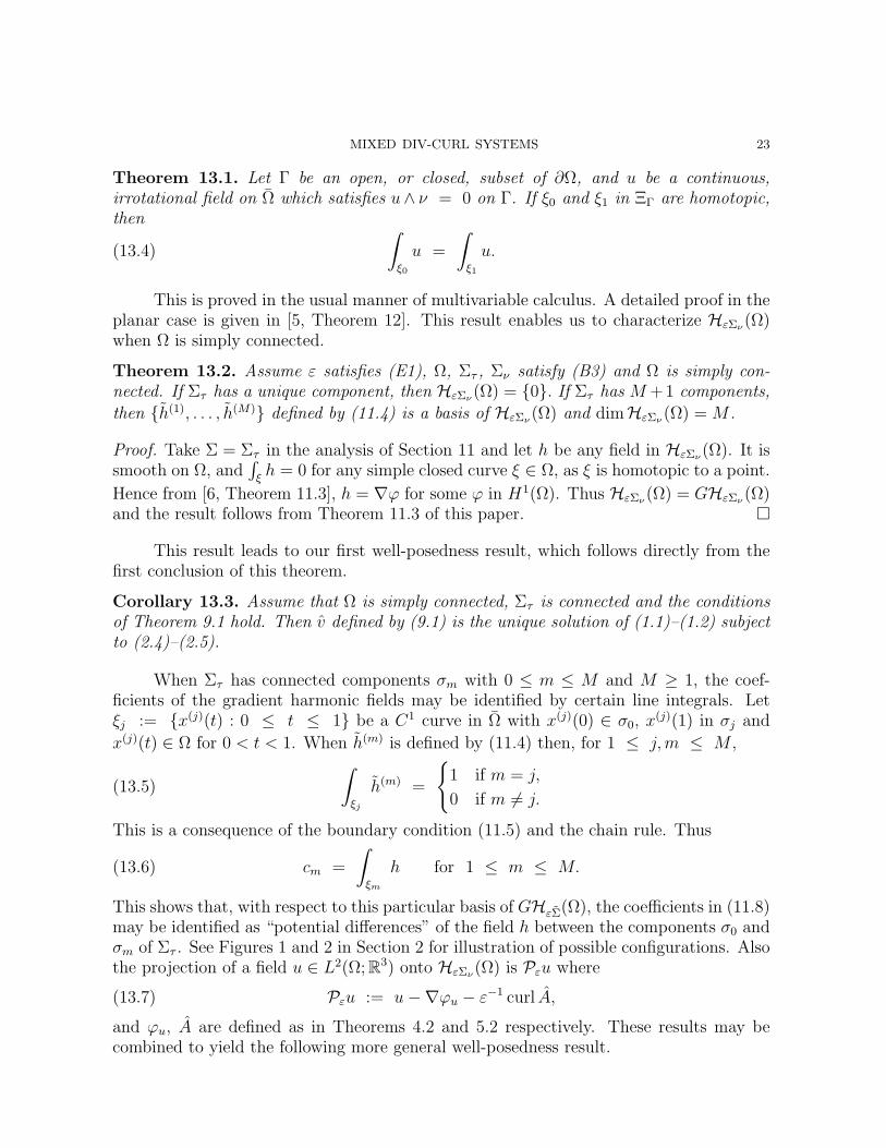
Corollary 13.4. Assume that Ω is simply connected, Στ has M+1 connected componentsand the conditions of Theorem 9.1 hold. Assume that the line integrals in equation (13.6)are prescribed for 1 ≤ m ≤ M where h is the field defined by (13.7) and the curvesξm : 1 ≤ m ≤ M are defined as above. Then there is a unique solution of (1.1)–(1.2)subject to (2.4)–(2.5) and (13.6).

Proof. From Corollary 9.2 and Theorem 13.2, the set of all solutions of (1.1)–(1.2)subject to (2.4)–(2.5) is given by (9.3) with k ∈ GHεΣν (Ω). Call this ε-harmonic field hinstead of k; then from equations (11.4) and (11.8), h is a smooth field on Ω from ellipticregularity theory for the associated boundary value problem for the scalar potentials χm.The above analysis shows that the coefficients in the representation (11.8) are determinedby the line integrals (13.6), so they determine a unique ε-harmonic component of thesolution as claimed.

Physically this result shows that a unique solution can be found provided one pre-scribes, in addition to the boundary data, M specific “potential differences” . That isby prescribing M special (equivalence classes of) line integrals of the field along pathsjoining different components of Στ . The values of these line integrals are independentof the specific path ξm chosen as a consequence of Theorem 13.1. A similar result couldbe stated where instead of (13.6), the fluxes hm defined by (11.10) are prescribed for theharmonic component of a field and for 1 ≤ m ≤M . When the region Ω has handles andΣτ has more than one component then the above functionals of the field determine thegradient component of the ε-harmonic field. It would be of considerable interest to knowwhat further functionals are required to uniquely determine the ε-harmonic componentsof solutions in this case.

The conclusion of this analysis is that to have a well-posed mixed div-curl problem,extra functionals of the solution may need to be prescribed in addition to the boundaryvalues. The number and type of these extra conditions depends on the differential topologyof the domain Ω and of the sets Στ and Σν where the different types of boundary dataare prescribed. A comprehensive theory has been described here for the case where Ω issimply connected. When the region Ω has handles, a number of open questions must beresolved before criteria for well-posedness can be described.

References

[1] A. Alonso and A. Valli, “Some remarks on the characterization of the space of tangential tracesof H(rot; Ω) and the construction of an extension operator,” Manus. Math. 89 (1996), 159-178.

[2] G. Auchmuty, “Orthogonal Decompositions and Bases for three-dimensional Vector Fields,” Nu-mer. Funct. Anal. Optimiz. 15 (1994), 445-488.

[3] G. Auchmuty, “The main inequality of 3d vector analysis,” Math Modelling & Methods in Appl.Sciences, 14 (2004), 79-103

[4] G. Auchmuty, “Trace results for mixed boundary value problems,” in preparation.


[5] G. Auchmuty and J.C. Alexander, “L2-well-posedness of planar div-curl systems,” Arch. Rat.Mech. & Anal., 160 (2001), 91-134.

[6] G. Auchmuty and J.C. Alexander, “L2-well-posedness of 3d div-curl systems on bounded regions,”Quart. J. Appl. Math. (in press).

[7] P. Blanchard and E. Bruning, Variational Methods in Mathematical Physics, Springer Verlag,Berlin (1992).

[8] R. Dautray and J. L. Lions, Mathematical Analysis and Numerical Methods for Science andTechnology, 6 volumes, Springer Verlag, Berlin (1990).

[9] P. Fernandes and G. Gilardi, “Magnetostatic and electrostatic problems in inhomogeneousanisotropic media with irregular boundary and mixed boundary conditions,” Math. Models andMethods in Applied Sciences, 7 (1997), 957-991.

[10] G.W. Hanson and A.B. Yakovlev, Operator Theory for Electromagnetics, Springer, New York(2002).

[11] J.D. Jackson, Classical Electrodynamics, John Wiley, New York (1962).[12] E.P. Stephan, “Boundary integral methods for mixed boundary value problems in R3,” Math.

Nach., 134 (1987), 21-53.[13] J. Wloka, Partial Differential Equations, Cambridge University Press, (1987).[14] E. Zeidler, Nonlinear Functional Analysis and its Applications, III: Variational Methods and

Optimization, Springer Verlag, New York (1985).

Division of Mathematical Sciences, National Science Foundation,, 4201 WilsonBlvd,, Arlington, Va 22230, USA

E-mail address: [email protected]

Department of Mathematics, Case Western Reserve University, 10900 Euclid Av-enue, Cleveland, OH 44106-7058, USA

E-mail address: [email protected]

Documents

FINITE ENERGY SOLUTIONS OF MIXED 3D DIV-CURL SYSTEMS