Finite Element Method A Perfectly Matched Layer for

Computational Electromagnetics Team: Aaron Smull (Undergraduate, ECE)

Ana Manic (Graduate, ECE)

Sanja Manic (Graduate, ECE)

Advisor: Dr. Branislav Notaros

Overview

I. Finite Element Method and Computational Electromagnetics

II. Project Goals

III. Theoretical Modeling in FEM

IV. Anisotropic and Inhomogeneous Media

V. Boundary Conditions and the Perfectly Matched Layer

VI. Applications

VII. Budget

VIII. Future Plans

Finite Element Method (FEM) in Computational Electromagnetics

www.ansys.com

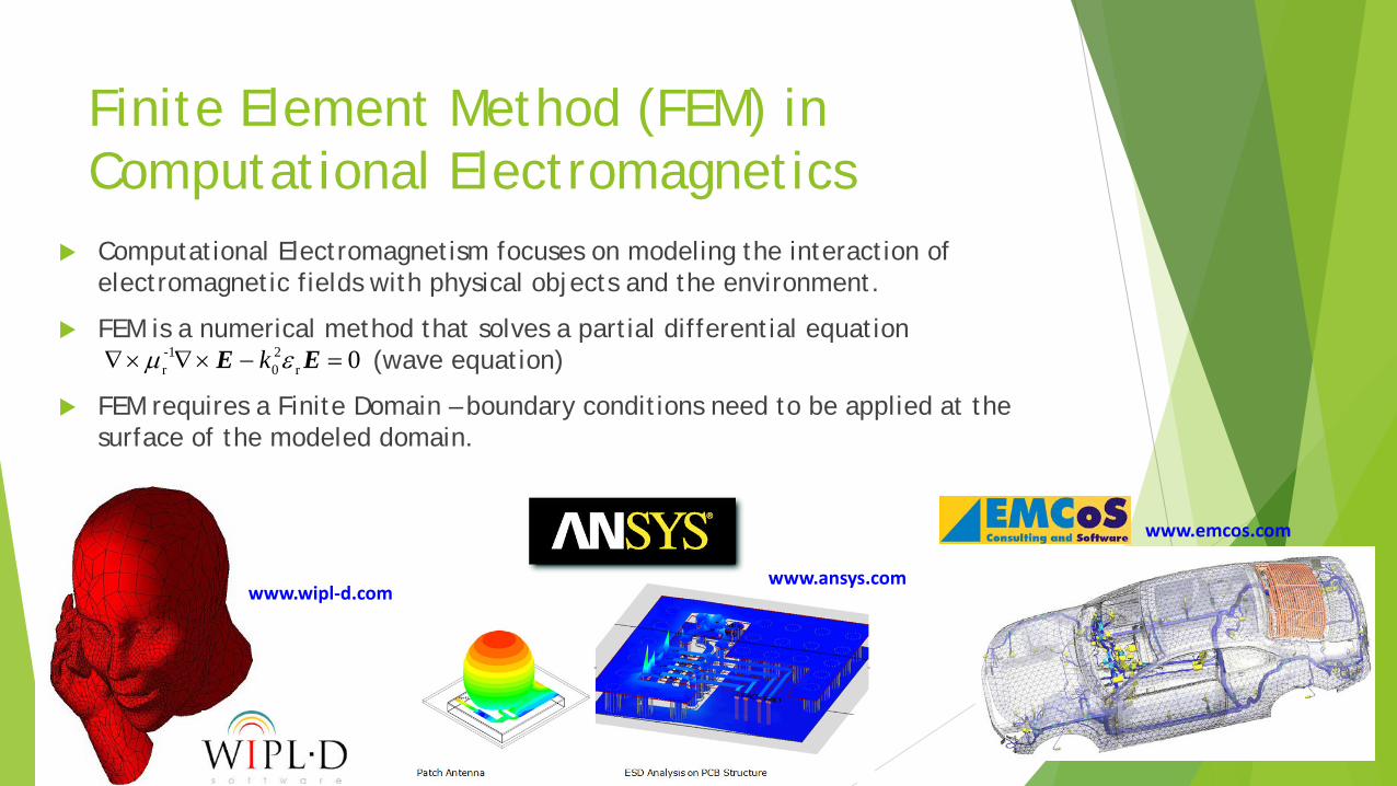
Computational Electromagnetism focuses on modeling the interaction of electromagnetic fields with physical objects and the environment.

FEM is a numerical method that solves a partial differential equation (wave equation)

FEM requires a Finite Domain – boundary conditions need to be applied at the surface of the modeled domain.

0r20

-1r =−×∇×∇ EE εµ k

www.emcos.com

www.wipl-d.com

Project Goals

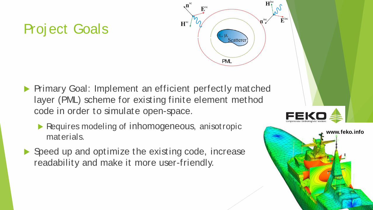
Primary Goal: Implement an efficient perfectly matched layer (PML) scheme for existing finite element method code in order to simulate open-space.

Requires modeling of inhomogeneous, anisotropic materials.

Speed up and optimize the existing code, increase readability and make it more user-friendly.

www.feko.info

PML

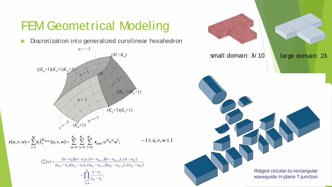
FEM Geometrical Modeling Discretization into generalized curvilinear hexahedron

;

))...()()...()(())...()()...()((

)(

0

1110

1110

∏≠=

+−

+−

−

−=

−−−−−−−−−−

=

K

mjj jm

j

Kmmmmmmm

KmmKm

uuuu

uuuuuuuuuuuuuuuuuuuuuL

; ),,(ˆ),,(0001

lnmmnl

K

l

K

n

K

m

M

i

Kii wvuwvuLwvu

wvuuvw rrr ∑∑∑∑

====== 1,,1 ≤≤− wvu

Ridged circular-to-rectangular waveguide H-plane T-junction

large domain: 2λ small domain: λ/10

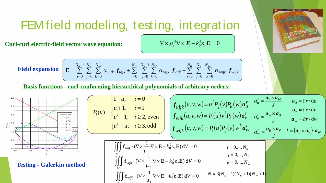
FEM field modeling, testing, integration

( ) ( ) ( ) rukj

iuijk wPvPuwvu af ,, =

Juwr

vaaa ×

=

Jwvr

uaaa ×

=

Jvur

waaa ×

=

uu d/ra ∂=

ww d/ra ∂=

vv d/ra ∂=

( ) wvuJ aaa ⋅×=

( ) ( ) ( ) rvk

iivijk wPvuPwvu af ,, =

( ) ( ) ( ) rw

kjiwijk wvPuPwvu af ,, =

wijkwijk

N

k

N

j

N

ivijkvijk

N

k

N

j

N

iuijkuijk

N

k

N

j

N

i

wvuwvuwvufffE

1

0000

1

0000

1

0α+α+α= ∑∑∑∑∑∑∑∑∑

−

====

−

====

−

=

Basis functions - curl-conforming hierarchical polynomials of arbitrary orders:

Testing - Galerkin method

0r20

-1r =−×∇×∇ EE εµ kCurl-curl electric-field vector wave equation:

Field expansion

0d )1( r20

r=ε−×∇

µ×∇⋅∫∫∫

Vuijk Vk EEf

0d )1( r20

r=ε−×∇

µ×∇⋅∫∫∫

Vvijk Vk EEf

0d )1( r20

r=ε−×∇

µ×∇⋅∫∫∫

Vwijk Vk EEf

w

v

u

NkNjNi

,...,0,...,0,...,0

===

)1)(1)(1(3 +++= wvu NNNN

≥−≥−=+=−

=

odd ,3,even ,2,1

1,10,1

)(

iuuiuiuiu

uP

i

ii

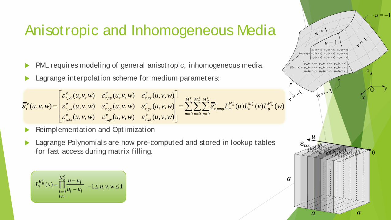
Anisotropic and Inhomogeneous Media

PML requires modeling of general anisotropic, inhomogeneous media.

Lagrange interpolation scheme for medium parameters:

Reimplementation and Optimization

Lagrange Polynomials are now pre-computed and stored in lookup tables for fast access during matrix filling.

∑∑∑= = =

=

=eu

ev

ew e

wev

eu

M

m

M

n

M

p

Mp

Mn

Mm

emnp

ezz

ezy

ezx

eyz

eyy

eyx

exz

exy

exx

e wLvLuLwvuwvuwvuwvuwvuwvuwvuwvuwvu

wvu0 0 0

r,

r,r,r,

r,r,r,

r,r,r,

r )()()(),,(),,(),,(),,(),,(),,(),,(),,(),,(

),,( εεεεεεεεεε

ε

∏≠= −

−=

eue

uK

ill li

lKi uu

uuuL0

)( 1,,1 ≤≤− wvu

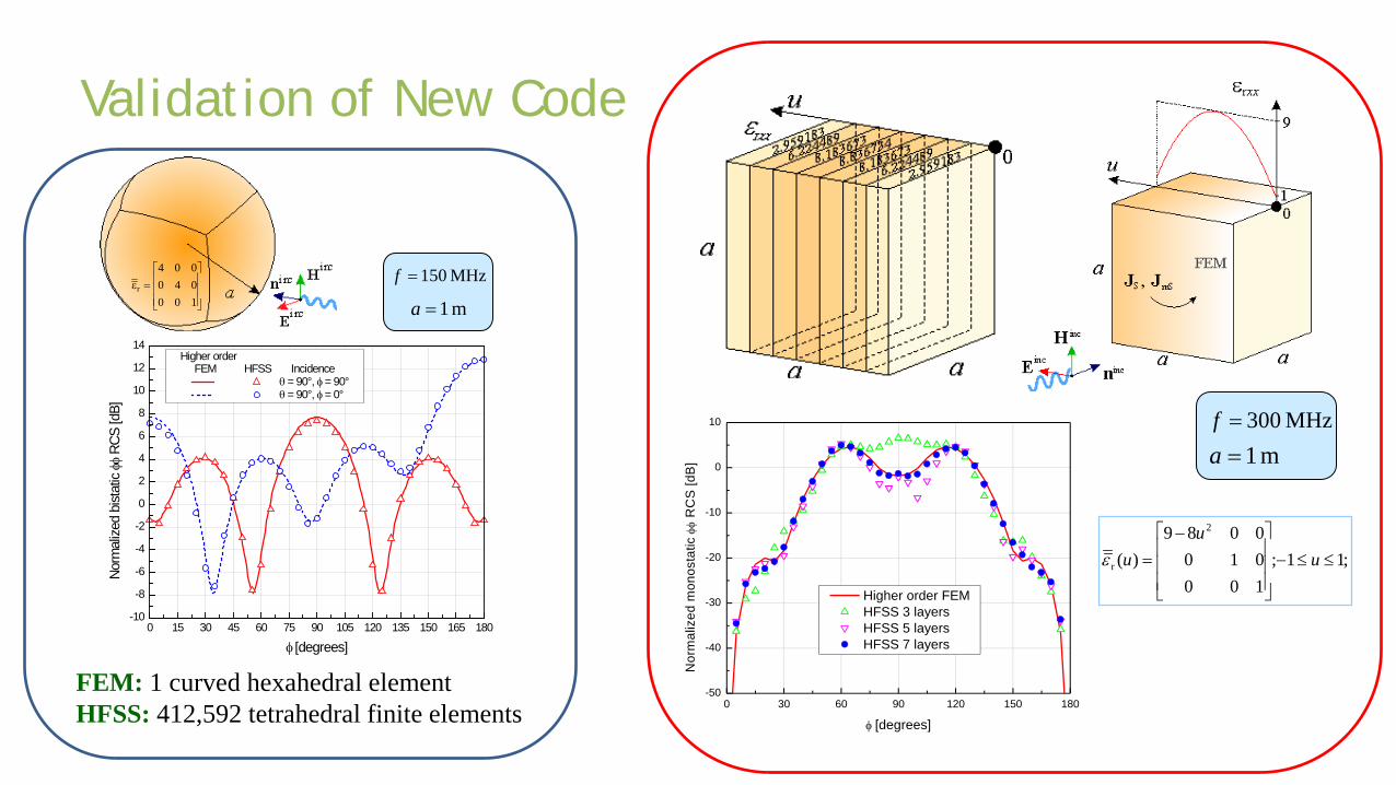
Validation of New Code

0 30 60 90 120 150 180-50

-40

-30

-20

-10

0

10

Nor

mal

ized

mon

osta

tic φ

φ R

CS

[dB

]

φ [degrees]

Higher order FEM HFSS 3 layers HFSS 5 layers HFSS 7 layers

m 1=aMHz 300=f

0 15 30 45 60 75 90 105 120 135 150 165 180-10

-8

-6

-4

-2

0

2

4

6

8

10

12

14

Norm

alize

d bi

stat

ic φφ

RCS

[dB]

φ [degrees]

Higher order FEM HFSS Incidence θ = 90°, φ = 90° θ = 90°, φ = 0°

=ε

100040004

r

m 1=a

MHz 150=f

;11;1000100089

)(

2

r ≤≤−

−= u

uuε

FEM: 1 curved hexahedral element HFSS: 412,592 tetrahedral finite elements

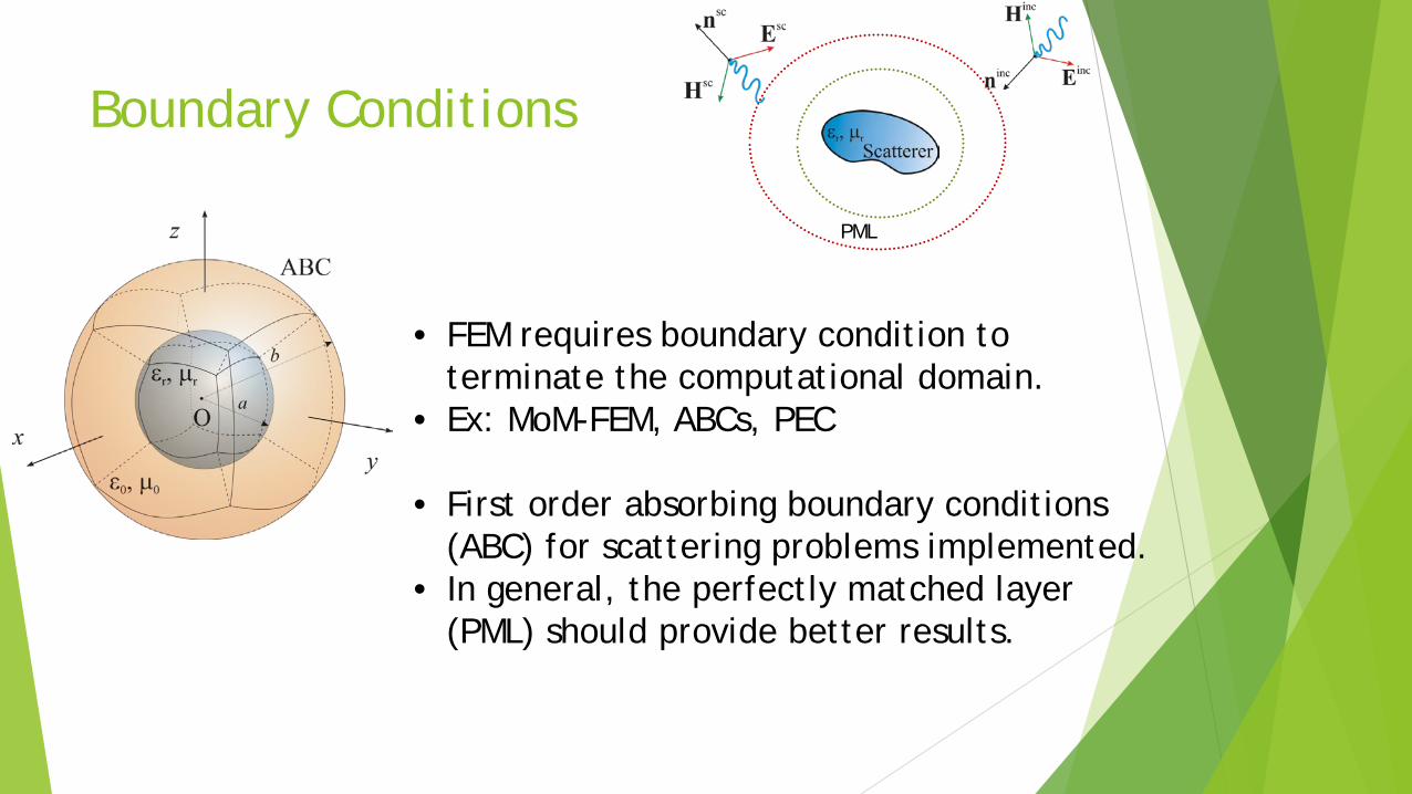
Boundary Conditions

• FEM requires boundary condition to terminate the computational domain.

• Ex: MoM-FEM, ABCs, PEC

• First order absorbing boundary conditions (ABC) for scattering problems implemented.

• In general, the perfectly matched layer (PML) should provide better results.

PML

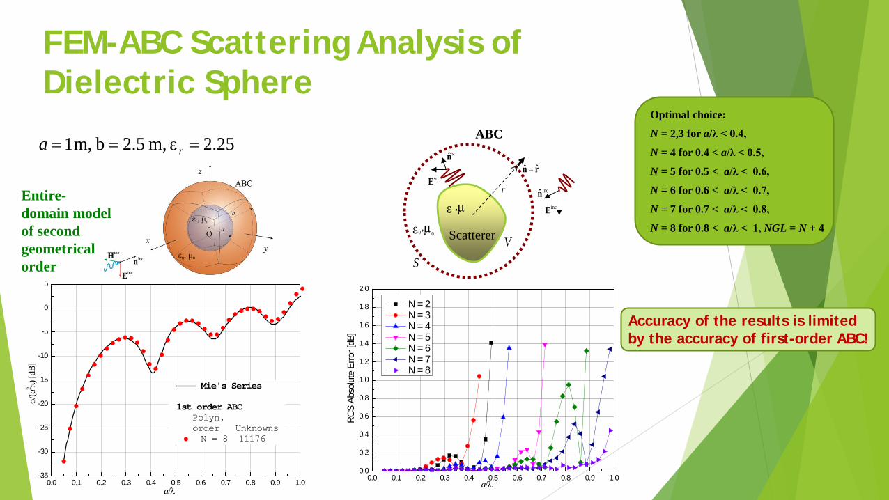
FEM-ABC Scattering Analysis of Dielectric Sphere

0.0 0.1 0.2 0.3 0.4 0.5 0.6 0.7 0.8 0.9 1.00.0

0.2

0.4

0.6

0.8

1.0

1.2

1.4

1.6

1.8

2.0

RCS

Abso

lute

Erro

r [dB

]

a/λ

N = 2 N = 3 N = 4 N = 5 N = 6 N = 7 N = 8

0.0 0.1 0.2 0.3 0.4 0.5 0.6 0.7 0.8 0.9 1.0-35

-30

-25

-20

-15

-10

-5

0

5

Mie's Series

1st order ABC Polyn. order Unknowns

N = 8 11176

σ/(a

2 π) [d

B]

a/λ

25.2m,2.5bm,1 =ε== ra

Optimal choice:

N = 2,3 for a/λ < 0.4,

N = 4 for 0.4 < a/λ < 0.5,

N = 5 for 0.5 < a/λ < 0.6,

N = 6 for 0.6 < a/λ < 0.7,

N = 7 for 0.7 < a/λ < 0.8,

N = 8 for 0.8 < a/λ < 1, NGL = N + 4

Entire-domain model of second geometrical order

V

Scatterer

µε ,

rn ˆˆ =

SV

µε 00 ,

rincE

incn̂

scn̂

scE

ABC

Accuracy of the results is limited by the accuracy of first-order ABC!

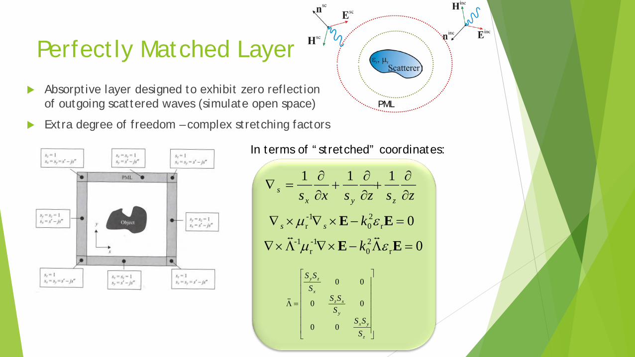
Perfectly Matched Layer

Absorptive layer designed to exhibit zero reflection of outgoing scattered waves (simulate open space)

Extra degree of freedom – complex stretching factors

zszsxs zyxs ∂

∂+

∂∂

+∂∂

=∇111

0r20

-1r =−×∇×∇ EE εµ kss

0r20

-1r

-1 =Λ−×∇Λ×∇ EE εµ

k

In terms of “stretched” coordinates:

=Λ

z

yx

y

xz

x

zy

SSS

SSS

SSS

00

00

00

PML

Current Work: Reformulation of The Wave Equation

Existence of the PML requires theoretical reformulation of our usual method.

Attenuating media does not allow wave excitation from the outside.

Unknowns are now coefficients for the scattered field, rather than the total field

SVkVScS

Incidentkji

V

Incidentkji

V

Incidentkji ∫∫∫ ⋅×∇×−⋅−×∇⋅×∇ d d d )()( -1

rˆˆ̂rˆˆ̂20

-1rˆˆ̂ EfEfEf µεµ

=⋅×∇×−⋅−×∇⋅×∇ ∫∫∫ SVkVDS

Scatteredkji

V

Scatteredkji

V

Scatteredkji d d d )()( -1

rˆˆ̂rˆˆ̂20

-1rˆˆ̂ EfEfEf µεµ

IncidentIncidentScatteredScattered kk EEEE r20

-1rr

20

-1r εµεµ

−×∇×∇=−×∇×∇

[ ] [ ] [ ]( ){ } { } { } { }IncidentIncidentIncidentScattered SBkASBkA −−=−− 20

20 α

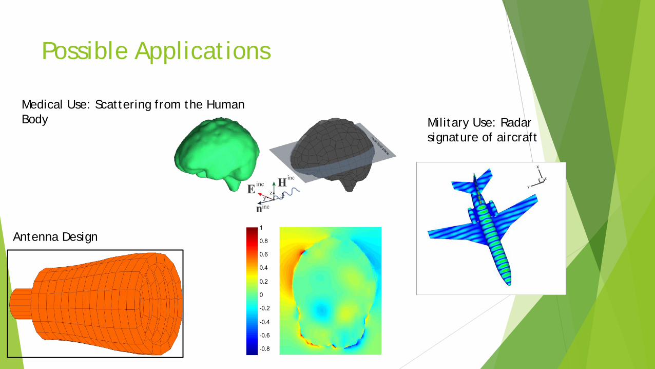
Possible Applications

Medical Use: Scattering from the Human Body

Antenna Design

Military Use: Radar signature of aircraft

Budget ECE Senior Design Budget: $100 Cost for second semester presentation <$10 for poster materials All other costs are covered; development tools are licensed by

CSU.

Continuation of PML Implementation

Extension of project to include conformal PML and possibly second order PML

Extensive testing of scattering structures to determine optimal PML parameters

Further Code Optimizations

Future Plans

References

[1] Ilić, M. “Higher order hexahedral finite elements for electromagnetic modeling”, University of Massachusetts Dartmouth, May 2003.

[2] M. M. Ilic and B. M. Notaros, “Higher order large-domain hierarchical FEM technique for electromagnetic modeling using Legendre basis functions on generalized hexahedra,” Electromagnetics, vol. 26, no. 7, pp. 517–529, Oct. 2006.

[3] Jin, J. M. and D. J. Riley, Finite Element Analysis of Antennas and Arrays, John Wiley & Sons, New York, 2008.

[4] Jin, J. M., Theory and Computation of Electromagnetic Fields, Wiley, 2010.

[5] Elene Chobanyan, PhD Dissertation Defense Presentation, December 1, 2014

[6] http://www-sop.inria.fr/nachos/