Embed Size (px)
Citation preview
FINITE ELEMENT DECOMPOSITION
OF THE HUMAN NEOCORTEX
A Thesis
by
SEELING CHOW
Submitted to the Office of Graduate Studies of Texas A&M University
in partial fulfillment of the requirements for the degree of
MASTER OF SCIENCE
May 1998
Major Subject: Computer Science
FINITE ELEMENT DECOMPOSITION
OF THE HUMAN NEOCORTEX
A Thesis
by
SEELING CHOW
Submitted to Texas A&M University
in partial fulfillment of the requirements for the degree of
MASTER OF SCIENCE
Approved as to style and content by:
May 1998
Major Subject: Computer Science
__________________________ Bruce H. McCormick (Chair of Committee)
__________________________ Ian S. Russell
(Member)
__________________________ Wei Zhao
(Interim Head of Department)
__________________________ Donald H. House
(Member)
__________________________ Nancy M. Amato
(Member)
iii
ABSTRACT
Finite Element Decomposition of the Human Neocortex.
(May 1998)
Seeling Chow, B.S., Texas A&M University
Chair Advisory Committee: Dr. Bruce H. McCormick
The finite element decomposition of the human neocortex provides a structural
information framework for the visualization and spatial organization of the neocortex at
progressive levels of detail. The decomposition satisfies neuroanatomical consistency, a
set of constraints defined by neuroanatomists' needs, the anatomical structure of the
brain, and the positioning of neurons inside the neocortical tissue. The finite elements
provide the boundaries for numerical grid generators to establish boundary-conforming
local coordinate systems for the systematic study and visualization of cortical neuron
populations. The decomposition method is implemented with a newly developed set of
object-oriented software tools.

iv
To my parents

v
ACKNOWLEDGEMENTS
I would like to thank Dr. Bruce McCormick for his invaluable guidance, inestimable
insight, and encouragement. His vision provided the basis for many of the ideas in this
thesis. I thank Dr. Nancy Amato for her moral support and personal advice throughout
my graduate course work. Also, I thank Dr. Donald House for introducing me to the
wonderful possibilities of computer graphical visualization and Dr. Ian Russell for his
expertise and excitement for neuroanatomy. I extend my gratitude to Leonardo Borges
for his supportive friendship and the memorable times at the laboratory. I thank my
peers Michael Stembera, Brent Burton, Burchan Bayazit, and Michael Nichols for the
good times in graduate school. I thank Suzanne for her compassion and persistence
throughout the development of this thesis. Finally, I thank my family for always being
there.
vi
TABLE OF CONTENTS
Page
ABSTRACT .......................................................................................................................iii
ACKNOWLEDGEMENTS ................................................................................................ v
TABLE OF CONTENTS ...................................................................................................vi
LIST OF FIGURES..........................................................................................................viii
CHAPTER
I INTRODUCTION................................................................................................... 1
A. Structural Information Frameworks ............................................................ 2 B. Finite Element Mesh as Structural Information Framework....................... 5 C. Objectives .................................................................................................... 7
II 3D SURFACE RECONSTRUCTION .................................................................. 10
A. Introduction ............................................................................................... 10 B. The Reconstruction Process ...................................................................... 11 C. Reconstruction Based on Delaunay Triangulation .................................... 12
III FEATURE EXTRACTION................................................................................... 20
A. Introduction ............................................................................................... 20 B. Principal Curvatures .................................................................................. 21 C. Shape Metrics from Principal Curvatures ................................................. 26 D. Topological and Geometric Features......................................................... 30
IV B-SPLINE TENSOR PATCHES .......................................................................... 34
A. Introduction ............................................................................................... 34 B. B-spline Tensor Product ............................................................................ 35 C. Smoothing Criterion .................................................................................. 37 D. Smooth Surface Fitting over a Rectangular Domain................................. 39 E. Blending B-spline Tensor Product Patches ............................................... 42
vii
Page V OVERVIEW OF NEOCORTICAL FINITE ELEMENT DECOMPOSITION ...45
A. Introduction to Finite Element Mesh Generation...................................... 45 B. The Neocortical Finite Element Decomposition Problem......................... 46 C. Methodology for Neocortical Finite Element Decomposition .................. 52 D. Decomposition into Macro Elements ........................................................ 55
VI METHODOLOGY................................................................................................ 59
A. Anatomical Division into Major Gyri ....................................................... 59 B. Decomposition of Gyral Folds into Macro Elements................................ 60 C. Reparameterization of Macro Elements .................................................... 62 D. Construction of Hexahedral Macro Elements ........................................... 68 E. Division into Hexahedral Finite Elements ................................................ 71
VII OBJECT-ORIENTED SOFTWARE TOOLS....................................................... 72
A. Introduction ............................................................................................... 72 B. Brief Descriptions of Software Tools........................................................ 72 C. Application of Software Tools to the Human Neocortex.......................... 74
VIII RESULTS.............................................................................................................. 77
A. Contour Extraction .................................................................................... 77 B. Solid Model Reconstruction of the Right Hemisphere ............................. 80 C. Extraction of Middle Temporal Gyrus ...................................................... 86 D. Macro Element Decomposition................................................................. 87 E. Feature Extraction for Reparameterization ............................................... 87 F. Finite Element Decomposition.................................................................. 94
IX SUMMARY AND FUTURE WORK................................................................. 101
A. Summary ................................................................................................. 101 B. Future Work ............................................................................................ 101
REFERENCES................................................................................................................ 105 VITA ............................................................................................................................... 110
viii
LIST OF FIGURES
FIGURE Page
1 Reconstruction stages ..............................................................................................11
2 Voronoi diagram and Delaunay triangulation .........................................................13
3 IVS and EVS of two contours .................................................................................15
4 Nearest neighbor to circumcenter............................................................................16
5 Three types of tetrahedra in 3D Delaunay triangulation .........................................17
6 Non-solid connections .............................................................................................17
7 Inserting internal points...........................................................................................18
8 Finding normal curvature for curve Ci ....................................................................22
9 Construction of a bivariate polynomial ...................................................................26
10 Unfolding a vertex and its incident angles ..............................................................28
11 Four types of topological regions ............................................................................31
12 Smoothing function Fg,h(p)......................................................................................41
13 Blending Surface .....................................................................................................43
14 Neurons implanted inside a neocortical finite element ...........................................47
15 Grid generated local coordinate system within a neocortical finite element...........................................................................................................47
16 Representation of a finite element...........................................................................48
17 Three types of dividing boundaries for neuroanatomical consistency ..............................................................................................................51
18 Mapping a template onto the object domain ...........................................................53

ix
FIGURE Page
19 Hierarchical division of the human brain into its anatomical parts .........................................................................................................................54
20 Decomposition of a major gyrus into macro elements............................................56
21 Different gyral shapes and their lines of symmetry.................................................57
22 Mapping gyral line of symmetry at different levels of detail..................................58
23 Sectional view in human brain atlas........................................................................60
24 Relationships between iso-parametric curves and principal curvature directions .................................................................................................63
25 Reparameterizing macro elements for finite element decomposition .........................................................................................................69
26 Propagation of reference template to tensor product parameter space .......................................................................................................70
27 Extracted contours for the exterior and interior surfaces of the human neocortex .....................................................................................................78
28 Ten contours for the exterior neocortical surface of the right hemisphere cross-sectioned through the coronal plane at 0.7mm thickness......................................................................................................79
29 Sagittal view of the reconstructed exterior neocortical surface of the right hemisphere............................................................................................81
30 Sagittal view of the reconstructed interior neocortical surface of the right hemisphere............................................................................................82
31 Angular view of the reconstructed neocortex of the right hemisphere ..............................................................................................................83
32 Front view of the reconstructed neocortex cut through the coronal plane at 38mm from the back .....................................................................84
33 Front, top, bottom, left, and right views of the reconstructed neocortex cut through the coronal plane at 38mm from the back .........................................................................................................................85

x
FIGURE Page
34 Middle Temporal Gyrus extracted from the Delaunay triangulation of the neocortex of the right hemisphere ...........................................86
35 Determining the gyral line of symmetry for the exterior surface of the Middle Temporal Gyrus ...................................................................88
36 Determining the gyral line of symmetry for the interior surface of the Middle Temporal Gyrus ...................................................................89
37 Exterior surface of the Middle Temporal Gyrus decomposed into six quadrilateral macro elements......................................................................90
38 Interior surface of the Middle Temporal Gyrus decomposed into six quadrilateral macro elements......................................................................91
39 Feature extraction for reparameterization ...............................................................92
40 Shape index color mapped onto the surface of a gyrus ...........................................93
41 Constructing hexahedral finite elements .................................................................95
42 Neuroanatomically consistent finite elements for a segment of the Middle Temporal Gyrus................................................................................96
43 Neuroanatomically consistent finite elements for a segment of the Middle Temporal Gyrus (bottom view) ........................................................97
44 Neuroanatomically consistent finite elements for the Middle Temporal Gyrus (side view)....................................................................................98
45 Neuroanatomically consistent finite elements for the Middle Temporal Gyrus (bottom view)...............................................................................99
46 Neuroanatomically consistent finite elements for the Middle Temporal Gyrus (front view) ................................................................................100
1
CHAPTER I
INTRODUCTION
Neuroscience research has precipitated a rising influx of visual information in need
of an organizing framework. A vast repository of information is accumulating from the
various contributing fields, e.g. computational neuroscience, visualization-based
neuroanatomy, and functional imaging. Biomedical imaging techniques, such as MRI
and brain cryosectioning, are pouring forth a plethora of anatomical data, while
researchers in brain mapping are making significant advances in collecting functional-
structural data using fMRI. This agglomeration of valuable information lacks an
organizing framework by which to manage, visualize, analyze, model, and distribute the
information at both global and local levels of detail. Researchers in structural
informatics term this organizational void as the need for a structural information
framework [11]. Their definition encompasses a spatial-structural model for the
brain along with other media sources, such as journal literature, experimental findings,
and conceptual models. We concern ourselves with the core of the structural
information framework: a spatial organizational framework for the human brain.
Finite element mesh generation, a technique long practiced in fluid mechanics and
computational physics and an emerging discipline in computer aided geometric design
(CAGD), decomposes a spatial object into manageable sub-components. The
parcellation, in conjunction with supporting data structures, establishes a spatial database
Journal model is IEEE Transactions on Visualization and Computer Graphics.
2
useful for the management, analysis, and visualization of functional-structural
information. The resultant scaffolding alleviates the limitations and combines the
advantages of current visualization and organizational techniques in computational
neuroscience. The finite element mesh functions as a structural information framework,
offering the benefits of 3D modeling and information visualization. Further, the finite
elements provide the scaffolding for a virtual reality environment where neuron
populations can be graphically modeled, producing a three-dimensional neuron
arboretum [4]. The 3D finite element mesh serves as the underlying framework behind
the exploratory and navigational system proposed in Exploring the Brain Forest [12].
This hierarchical environment coordinates the graphical modeling and structural
information management at both the tissue and cellular levels.
A. Structural Information Frameworks
Brain mapping is motivating the integration of 3D visualization with structural-
functional data in order to build a ubiquitous structural information framework.
Currently, the major contributing research projects include the Human Brain Project
(http://www.nimh.nih.gov/research/hbp.htm), the Voxel Man (http://users.ox.ac.uk/
~uzdl0037/voxman.html), the Visible Human (http://wardens.tamu.edu/images/
vishum.html), the Digital Anatomist (http://www7.biostr.washington.edu/slideshows/
Quickview/title.html), and Human Brain Mapping (http://www.journals.wiley.com/
wilcat-bin/ops/ID1/1065-9471/prod). The prevailing frameworks utilize both 2D and 3D
imaging techniques, each with its advantages and inherent limitations. Two emerging
structural information frameworks are flat maps and brain atlases.
3
The goal of flat mapping is synonymous to the mapmaker's problem, which is to find
a flat representation of a curved surface. With the aid of computer graphical modeling,
researchers have developed semi-automatic methods for unfolding the convoluted
cortical tissue into a flat (or ellipsoid) 2D map [53], [13], [18]. These techniques involve
the flattening of a polyhedral surface representation to an ellipsoidal or planar graph by
optimizing a distance metric that seeks to minimize distortion. Their efforts have
produced flat maps for the primary visual cortical area, labeled V1, of a macaque
monkey; the entire right hemisphere of layer 4 of the neocortex of a macaque monkey;
and the exterior cortical layer of a human brain. Flat maps ease visualization of the
convoluted tissue in many ways; they provide a gobal overview, simplify navigational
complexity, and preserve topological relationships along the surface representation. The
reduction of spatial complexity from 3D to 2D facilitates the organization and mapping
of functional information to the cortical surface [17]. However, flat maps pose inherent
limitations common to procedures that restrict complex 3D structures to 2D images.
Their surface-based approach discards the spatial structure among the layers within the
neocortex; furthermore, pressing the folded surface introduces additional distortion and
loss of spatial-structural information. The loss of spatial dimension can be partially
compensated with the color mapping of shape metrics onto the planar surface, but such
attempts complicates the mapping of functional information and ignores the benefits of
3D imaging of the brain as a volume.
Brain atlases overcome the limitations of flat maps by preserving the 3D
representation of the human brain. Much of their development stems from surgical
4
planning [59], [25], [35], teaching [60], modeling, and anatomical studies [19]. A brain
atlas is comprised of either a collection of carefully labeled serial cross sections or a 3D
reconstructed computer graphical model.
To produce sectional brain atlases, neuroanatomists have traditionally hand-drawn or
systematically photographed sections of the brain, manually extracting highly detailed
structures. Automatic labeling schemes applied to digitized drawings, such as forward
transforms [38], show promise for the use of sectional atlases as an organizing
framework, but the restricted 2D sectional viewing shares the limitations of flat maps for
visualization purposes. Researchers in functional imaging have extended sectional
viewing to the "corner cube environment," which simultaneously displays the coronal,
sagittal, and horizontal sections on the inner walls of a cube [52]. The superimposed
plots of brain activation data onto the voxels of the cube provide only the location of the
activation, leaving out the spatial structural information. In sum, sectional viewing
affords only restricted spatial relationships between functional and structural
information.
A more comprehensive and ambitious approach to brain atlas generation is the
reconstruction of serial cross sections into a 3D graphical model. Such 3D brain atlases
adopt two types of representation: voxel-based and surface-based. A voxel is the three-
dimensional equivalent of a pixel, and the construction of voxel-based atlases involves
the segmentation of a voxel dataset, the collection of digitized serial cross sections, into
anatomical sub-structures. Segmentation techniques often employ a priori knowledge,
human interaction, and statistical methods, such as Bayesian probability, to categorize
5
the voxels into appropriate anatomical parts. Researchers working on the Visible
Human project and the Voxel Man project have constructed 3D human brain atlases
utilizing these volume classification schemes [36]. The alternative approach is to
represent the anatomical structures as explicit surfaces. Most of the existent surface-
based atlases model the brain with polyhedral surfaces constructed using serial surface
reconstruction or conversion algorithms applied to the voxel datasets, e.g. the wrapper
algorithm [27] or the marching cubes algorithm [43]. Whether voxel-based or surface-
based, 3D brain atlases retain the spatial structural information, but they lack the global
overview and navigational simplicity flat maps provide. Maneuvering around the 3D
atlases demands a framework and an interface that provides more than just rotation,
translation, and labeling; effective navigation and visualization necessitates an
organizing framework currently lacking in these atlases.
B. Finite Element Mesh as Structural Information Framework
The exploratory environment in Exploring the Brain Forest [12] utilizes a structural
information framework that overcomes the limitations of brain atlases and flat maps.
Further, it facilitates experimental studies, structural and functional modeling,
simulations, and numerical analyses at progressive levels of detail: from the global
anatomy of the brain to segments of neocortical tissue embedded with 3D graphical
neurons. This structural information framework, based on a finite element (FE) mesh
generated from the human neocortex, provides the necessary hierarchical spatial
information management and 3D visualization system.
6
The neocortical finite element decomposition first partitions the brain into its four
anatomical lobes; at the next finer level of detail, the lobes are divided into their major
anatomical gyri. Next, the gryi are decomposed into macro elements and then each
macro element into finite elements. At the finest level of detail, numerical grid
generation within the wedge-shaped finite elements establishes a boundary-conforming,
three-dimensional local coordinate system. Then, each neuron in a neuron morphology
data repository, whether a traced biological neuron or a synthetically generated neuron,
can be assigned to the FE which contains its soma. The cerebral cortex, so modeled, can
be viewed as a giant �chest of drawers� where a �drawer� (any selected FE or cluster of
neighboring FEs) can be �opened� as a file and its population of neurons visualized.
These FEs therefore define a file structure isomorphic to the neocortex as modeled and
visualized at both cellular and tissue levels.
To build a neocortical finite element mesh, we developed and implemented a method
to decompose the neocortex into an unstructured grid of hexahedral finite elements; as a
result, the 3D mesh is a solid model of the neocortex, rather than just a surface model.
The decomposition is based on anatomical structures, such as sulci and gyri, the
traditional landmarks for anatomical registration and functional imaging. The parametric
boundaries of each hexahedral FE, defined by six surface patches, furnish the necessary
constraints to numerically generate 3D grids within the FE [4]. As described in
Exploring the Brain Forest, the finite element decomposition of the neocortex in
conjunction with grid generation provides a 3D visualization environment and an
information management system.

7
C. Objectives
The five objectives of this research are listed below:
1. 3D reconstruction of the neocortex
2. Feature extraction from the boundary representation model
3. Neuroanatomically-consistent finite element decomposition
4. Grid generation for the finite element model
5. Development of supplemental object-oriented software tools
C.1. 3D Reconstruction of the Neocortex
The first objective is to reconstruct a solid model of the human neocortex from cross-
sectional slices of a post mortem human brain. The dataset for the reconstruction
consists of 271 x 512 x 512 images of a 76-year-old normal female human cadaver brain
cryosectioned through the coronal plane [61]. Contours of the neocortex are manually
traced using a third party application (Elastic Reality from Avid Technologies, Inc.).
Then, a Delaunay-based surface reconstruction algorithm generates triangulated surfaces
for both the exterior and interior sides of the neocortical tissue. Thus, the inner and
outer surfaces jointly define the shell of the neocortex, producing a solid model called a
Boundary Representation (B-rep) in the field of Computer Aided Geometric Design
(CAGD).
C.2. Feature Extraction from the Boundary Representation Model
The second objective is to extract geometric and topological features from the B-rep
model. First, principal curvature values, defined loosely as the curvature of a point on a
8
surface, and their corresponding directional vectors are computed. Second, shape
metrics, such as intrinsic curvature and shape index, are derived from the principal
curvature information. Third, features, e.g. topological regions and extremal points, are
extracted using various search algorithms and filters.
C.3. Finite Element Decomposition
The third objective is to decompose the neocortical solid model into hexahedral
finite elements satisfying neuroanatomical consistency, a set of constraints defined by
neuroanatomists' needs, the anatomical structure of the brain, and the positioning of
neurons inside the neocortical tissue. The decomposition follows the mapped template
approach, requiring a coarse level partitioning into macro elements, or mapped
templates, and then the decomposition of finite elements within each macro element.
This approach is widely used in commercial CAGD software and provides a finite
element mesh closest to a rectangular grid. In addition to the boundaries of the solid
model, the finite element mesh conforms to the three boundaries suggested by
neuroanatomical consistency: major sulcal boundaries, gyral lines of symmetry, and
gyral ribs.
C.4. Grid Generation for the Finite Element Model
The fourth objective is to establish local curvilinear coordinate systems within the
finite elements of the solid model using numerical grid generators. Batte [4] has applied
3D ITTM grid generators and several 3D variational grid generators [37] to parametric
solid models of neocortical tissue segments. The finite element decomposition provides
9
the necessary boundary constraints for numerical grid generation inside the volume
defined by the six surfaces of a hexahedral finite element.
C.5. Object-Oriented Software for Finite Element Decomposition
The fifth objective is to develop object-oriented software tools compatible with
common graphical formats and adaptable to future research. The development of these
tools is based on a class library derived from the Visualization Tool Kit v1.3 (vtk) [56].
Our classes of geometric objects are directly compatible with the suite of software tools
included in vtk.
10
CHAPTER II
3D SURFACE RECONSTRUCTION
A. Introduction
Reconstructing a three-dimensional (3D) surface from a set of planar contours is a
common obstacle in biomedical imaging. Various imaging techniques in clinical
medicine, such as computed axial tomography (CAT), positron emission tomography
(PET), magnetic resonance imaging (MRI), and cryosectioning, provide a series of 2D
planar cross-sections. Motivated by the need for more interpretative visualization and
functional analysis, building 3D surface models through serial reconstruction has
received much attention in biomedical research [3], [8], [50]. Surface reconstruction
techniques include volume rendering, iso-surface algorithms, parametric surface fitting,
triangulation, and multiaxial triangulation, which optimizes triangulation by examining
sections taken through different cutting planes. Different methods offer their own
benefits and drawbacks ranging from robustness and computational requirements to
eloquence, aesthetic quality, compression, and representational value. For example, as
discussed in Chapter V, parametric representations offer boundary constraints for grid
generation. Users should select the reconstruction technique that best suits their needs.
One particular surface reconstruction technique, based on the Delaunay triangulation,
offers speed, robustness, and convenience. It combines the approaches of surface fitting
and voxel reconstruction techniques to produce a triangular mesh representation of the
3D surface model.
11
B. The Reconstruction Process
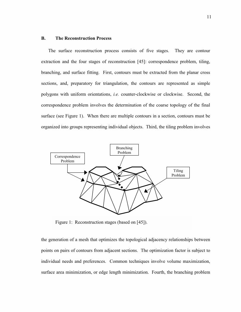
The surface reconstruction process consists of five stages. They are contour
extraction and the four stages of reconstruction [45]: correspondence problem, tiling,
branching, and surface fitting. First, contours must be extracted from the planar cross
sections, and, preparatory for triangulation, the contours are represented as simple
polygons with uniform orientations, i.e. counter-clockwise or clockwise. Second, the
correspondence problem involves the determination of the coarse topology of the final
surface (see Figure 1). When there are multiple contours in a section, contours must be
organized into groups representing individual objects. Third, the tiling problem involves
the generation of a mesh that optimizes the topological adjacency relationships between
points on pairs of contours from adjacent sections. The optimization factor is subject to
individual needs and preferences. Common techniques involve volume maximization,
surface area minimization, or edge length minimization. Fourth, the branching problem
Tiling Problem
Branching Problem
Correspondence Problem
Figure 1: Reconstruction stages (based on [45]).
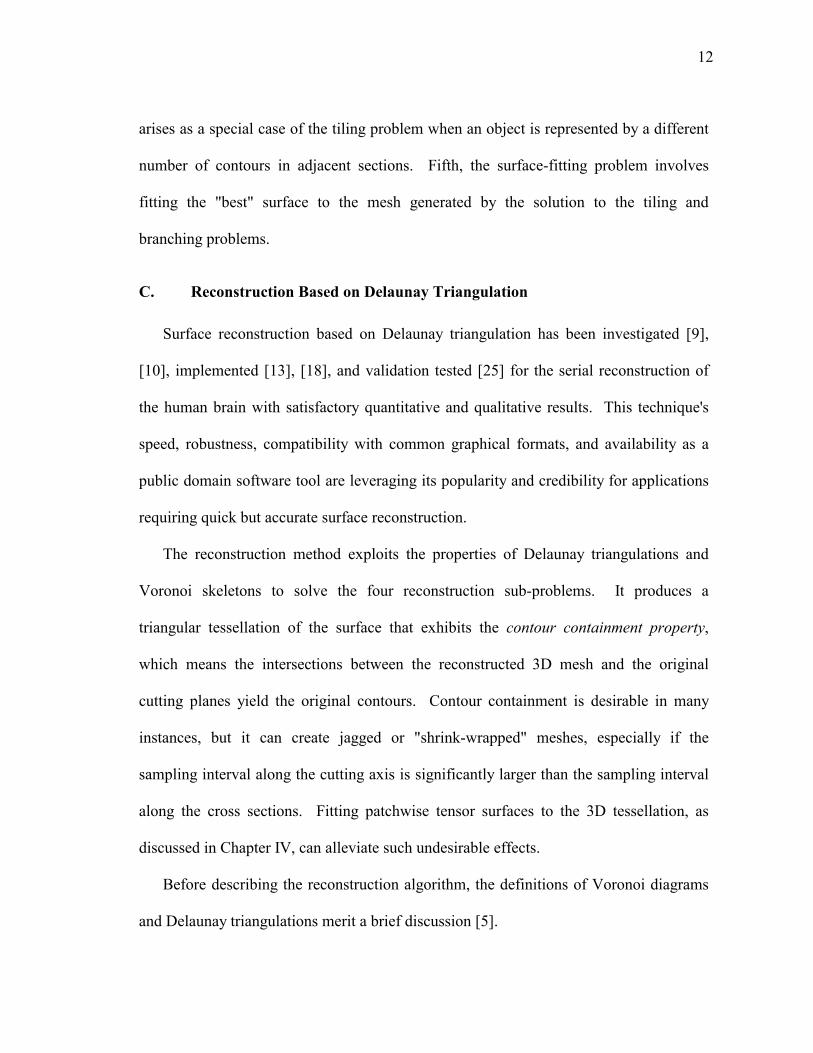
12
arises as a special case of the tiling problem when an object is represented by a different
number of contours in adjacent sections. Fifth, the surface-fitting problem involves
fitting the "best" surface to the mesh generated by the solution to the tiling and
branching problems.
C. Reconstruction Based on Delaunay Triangulation
Surface reconstruction based on Delaunay triangulation has been investigated [9],
[10], implemented [13], [18], and validation tested [25] for the serial reconstruction of
the human brain with satisfactory quantitative and qualitative results. This technique's
speed, robustness, compatibility with common graphical formats, and availability as a
public domain software tool are leveraging its popularity and credibility for applications
requiring quick but accurate surface reconstruction.
The reconstruction method exploits the properties of Delaunay triangulations and
Voronoi skeletons to solve the four reconstruction sub-problems. It produces a
triangular tessellation of the surface that exhibits the contour containment property,
which means the intersections between the reconstructed 3D mesh and the original
cutting planes yield the original contours. Contour containment is desirable in many
instances, but it can create jagged or "shrink-wrapped" meshes, especially if the
sampling interval along the cutting axis is significantly larger than the sampling interval
along the cross sections. Fitting patchwise tensor surfaces to the 3D tessellation, as
discussed in Chapter IV, can alleviate such undesirable effects.
Before describing the reconstruction algorithm, the definitions of Voronoi diagrams
and Delaunay triangulations merit a brief discussion [5].
13
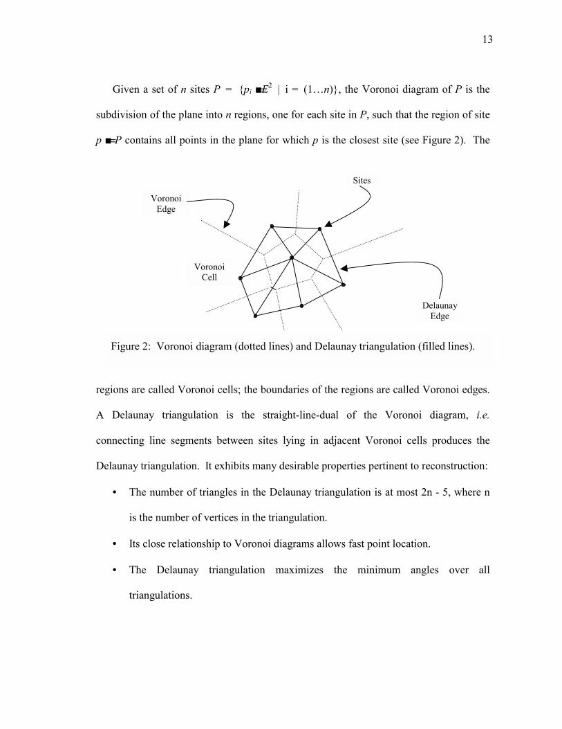
Given a set of n sites P = {pi É=E2 | i = (1�n)}, the Voronoi diagram of P is the
subdivision of the plane into n regions, one for each site in P, such that the region of site
p É= P contains all points in the plane for which p is the closest site (see Figure 2). The
regions are called Voronoi cells; the boundaries of the regions are called Voronoi edges.
A Delaunay triangulation is the straight-line-dual of the Voronoi diagram, i.e.
connecting line segments between sites lying in adjacent Voronoi cells produces the
Delaunay triangulation. It exhibits many desirable properties pertinent to reconstruction:
• The number of triangles in the Delaunay triangulation is at most 2n - 5, where n
is the number of vertices in the triangulation.
• Its close relationship to Voronoi diagrams allows fast point location.
• The Delaunay triangulation maximizes the minimum angles over all
triangulations.
Sites
Voronoi Cell
Voronoi Edge
DelaunayEdge
Figure 2: Voronoi diagram (dotted lines) and Delaunay triangulation (filled lines).
14
• Several algorithms are available to efficiently compute the Delaunay
triangulation [29], [39].
Hence, the Delaunay triangulation generates an efficient representation of the cross
sections, affords an angle-maximal surface tessellation, and has a worst case time
complexity of O(n2) with an expected time that increases linearly.
A detailed explanation of a reconstruction algorithm based on Delaunay triangulation
is provided in [10], [25]. It is summarized as follows:
1. Compute the 2D Delaunay triangulation of the vertices for each cross section.
2. Construct the Voronoi skeletons.
3. For each pair of adjacent cross sections do
3.1. Extend the two 2D triangulations to one 3D Delaunay triangulation.
3.2. Remove external tetrahedra and non-solid connections.
Step 1 of the algorithm is relatively straightforward given the numerous techniques
available for rapidly computing 2D Delaunay triangulations [5]. After determining the
Delaunay triangulation for a cross section, the method categorizes the Delaunay triangles
into internal and external triangles, depending on whether the triangles lie inside or
outside the contour. Then, step 2 of the algorithm constructs internal and external
Voronoi skeletons (IVS and EVS) for each group respectively. An IVS for a contour
consists of all the edges dual to an internal Delaunay edge, i.e. an edge shared by two
adjacent internal Delaunay triangles. By adaptively inserting points on the closed
polygon, the IVS converges to the medial axis as the number of points approaches
infinity. The medial axis of a polygon is the locus of points with equal distance to at
15
least two contour points; this feature is further discussed in [54]. An EVS for a cross
section is similar to the IVS, except edges are determined for adjacent external Delaunay
triangles (see Figure 3). In a sense, the EVS provides the partitioning of the contours
within a cross section. The Voronoi skeletons play a crucial role in the 3D
reconstruction.
Step 3 reduces surface reconstruction to computing a solid slice composed of
tetrahedra between each pair of adjacent cross sections. The procedure is synonymous
to sculpting a piece of hardwood. First, the contours mold a solid block without internal
details. Then, a chiseling process eliminates unwanted pieces, exposing the more
intricate form.
The solid block is, in fact, the 3D Delaunay triangulation of the vertices in a pair of
cross sections. It consists of three types of tetrahedra T1, T2, and T12 constructed through
a nearest-neighbor approach based on the circumcenter of a triangle. Given a pair of
adjacent 2D triangulated cross section P1 and P2, for each triangle t É= P1, the algorithm
EVS
IVS
Figure 3: IVS and EVS of two contours (based on [10]).
16
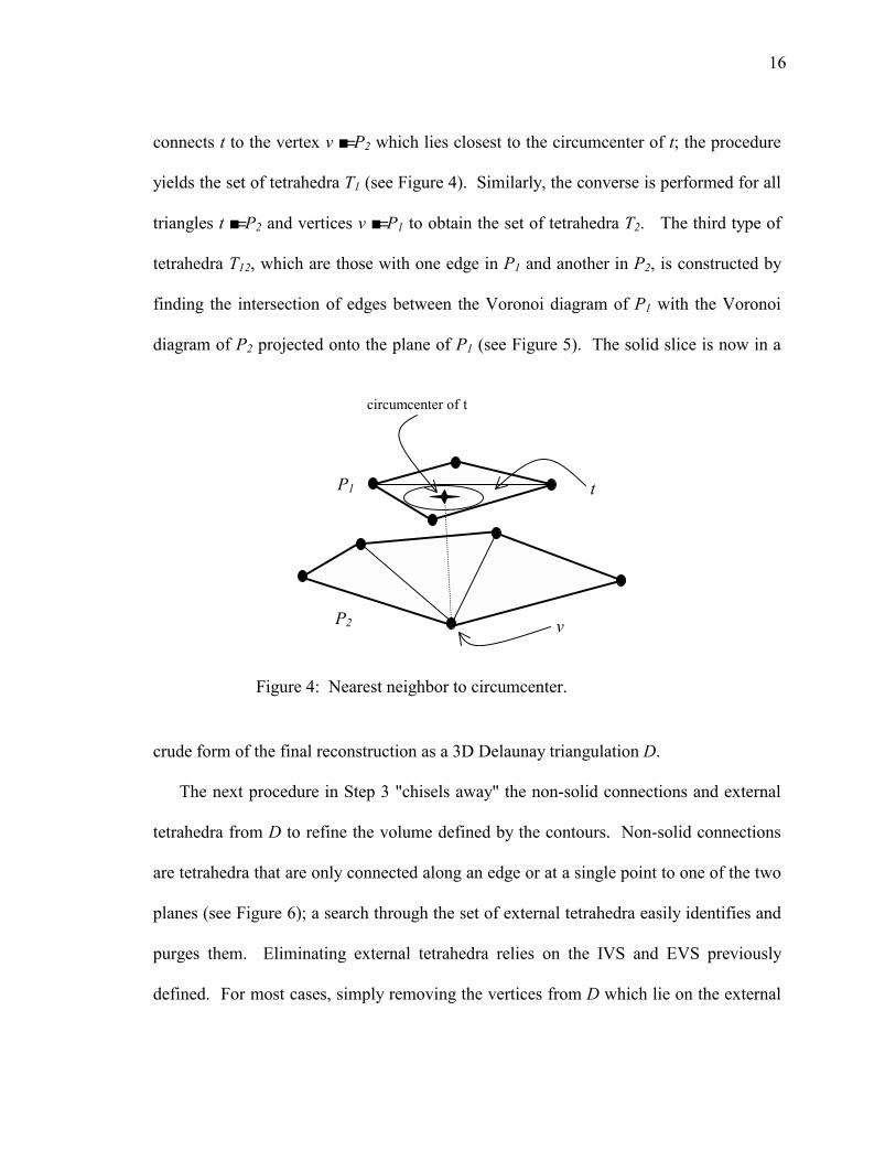
connects t to the vertex v É= P2 which lies closest to the circumcenter of t; the procedure
yields the set of tetrahedra T1 (see Figure 4). Similarly, the converse is performed for all
triangles t É= P2 and vertices v É= P1 to obtain the set of tetrahedra T2. The third type of
tetrahedra T12, which are those with one edge in P1 and another in P2, is constructed by
finding the intersection of edges between the Voronoi diagram of P1 with the Voronoi
diagram of P2 projected onto the plane of P1 (see Figure 5). The solid slice is now in a
crude form of the final reconstruction as a 3D Delaunay triangulation D.
The next procedure in Step 3 "chisels away" the non-solid connections and external
tetrahedra from D to refine the volume defined by the contours. Non-solid connections
are tetrahedra that are only connected along an edge or at a single point to one of the two
planes (see Figure 6); a search through the set of external tetrahedra easily identifies and
purges them. Eliminating external tetrahedra relies on the IVS and EVS previously
defined. For most cases, simply removing the vertices from D which lie on the external
P2
P1
v
t
circumcenter of t
Figure 4: Nearest neighbor to circumcenter.
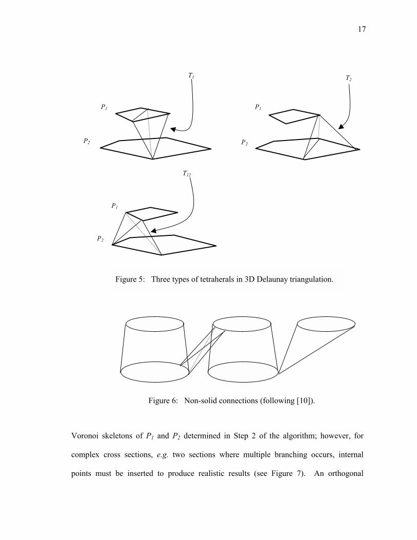
17
Voronoi skeletons of P1 and P2 determined in Step 2 of the algorithm; however, for
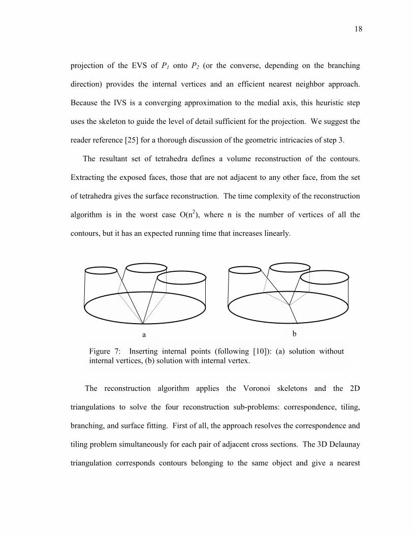
complex cross sections, e.g. two sections where multiple branching occurs, internal
points must be inserted to produce realistic results (see Figure 7). An orthogonal
T1
P2
P1
P2
T2
P1
T12
P2
P1
Figure 5:6 Three types of tetraherals in 3D Delaunay triangulation.
Figure 6:5 Non-solid connections (following [10]).
18
projection of the EVS of P1 onto P2 (or the converse, depending on the branching
direction) provides the internal vertices and an efficient nearest neighbor approach.
Because the IVS is a converging approximation to the medial axis, this heuristic step
uses the skeleton to guide the level of detail sufficient for the projection. We suggest the
reader reference [25] for a thorough discussion of the geometric intricacies of step 3.
The resultant set of tetrahedra defines a volume reconstruction of the contours.
Extracting the exposed faces, those that are not adjacent to any other face, from the set
of tetrahedra gives the surface reconstruction. The time complexity of the reconstruction
algorithm is in the worst case O(n2), where n is the number of vertices of all the
contours, but it has an expected running time that increases linearly.
The reconstruction algorithm applies the Voronoi skeletons and the 2D
triangulations to solve the four reconstruction sub-problems: correspondence, tiling,
branching, and surface fitting. First of all, the approach resolves the correspondence and
tiling problem simultaneously for each pair of adjacent cross sections. The 3D Delaunay
triangulation corresponds contours belonging to the same object and give a nearest
a b
Figure 7: Inserting internal points (following [10]): (a) solution withoutinternal vertices, (b) solution with internal vertex.
19
neighbor approach for optimizing topological adjacency. Second, the EVS projection
and insertion of internal vertices, as described above, resolve the branching problem.
Finally, the extracted surface from the volume reconstruction provides the solution to the
surface-fitting problem. The technique offers the "best" surface as an angle-optimal
triangular mesh exhibiting the contour containment property. Although the algorithm is
relatively robust, special cases can yield undesirable results, e.g. a non-manifold
triangulation or an artificial branching. One suggestion for reducing the complexity is to
solve the correspondence independently and then reconstruct each object separately.
Overall, the technique based on Delaunay triangulation offers a fast, robust, and
convenient reconstruction algorithm.
20
CHAPTER III
FEATURE EXTRACTION
A. Introduction
A feature is a region in a dataset that is of interest for its interpretation; feature
extraction is the extrication of these regions for further analysis and visualization.
Feature extraction has been investigated and utilized to solve a variety of problems, such
as shape matching [47], image registration [59], solid modeling [46], edge detection [2],
and data visualization [62]. In most of its applications, feature extraction provides a
compact representation of the relevant information embedded in the dataset.
Researchers define different types of features for their specific applications; hence,
they range from such simple definitions as intensity values of a 2D image to more
complex constructs such as mathematical transformations. When the dataset is a 2D or
3D image, Guan categorizes features into global/local and point/curve/surface
classifications [26]. Global features require calculations based on the whole image while
local features are derived from a limited area in the image. Point features include tie
points, anchor points, and extremal points; curve features include corner edges and ridge
lines; surface features include curvature and surface representation graphs.
The next three sections discuss the definition of principal curvatures and the
estimation of curvature values for polygonal meshes; some derived shape metrics; and
the features computed from principal curvature and directions.
21
B. Principal Curvatures
The principal curvatures for a point on a 2D manifold in Euclidean space are
properties fundamental to the differential geometry of parametric surfaces [14], [22];
consequently, the estimation of principal curvatures for triangulated surfaces rests on
these definitions. The estimating schemes rely on local approximations, employing
constructs such as the angle deficit [1], the Hessian matrix [28], and the osculating
paraboloid [31]. We discuss Hamann's technique, which locally fits a group of points to
an osculating paraboloid and computes the principal curvatures by solving a bivariate
polynomial.
For a point p0 on a regular parametric two-dimensional surface S in real three-
dimensional space �P, there exists a minimal normal curvature â min and maximal normal
curvature â max called the principal curvatures. Principal curvature is explained as
follows.
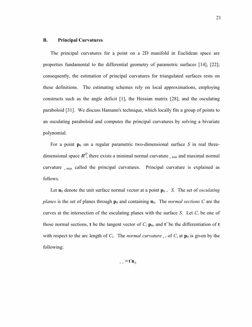
Let n0 denote the unit surface normal vector at a point p0 Ï S. The set of osculating
planes is the set of planes through p0 and containing n0. The normal sections C are the
curves at the intersection of the osculating planes with the surface S. Let Ci be one of
those normal sections, t be the tangent vector of Ci p0, and t¿ be the differentiation of t
with respect to the arc length of Ci. The normal curvature â i of Ci at p0 is given by the
following:
0 nt ′=iâ
22
The minimal and maximal normal curvatures of all the curves in the set C are then
and the principal curvature directions are tmin, the tangent vector of Ci at p0 with â i = â min,
and tmax, the tangent vector of Cj at p0 with â j = â max.
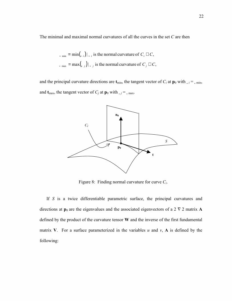
If S is a twice differentiable parametric surface, the principal curvatures and
directions at p0 are the eigenvalues and the associated eigenvectors of a 2 “ 2 matrix A
defined by the product of the curvature tensor W and the inverse of the first fundamental
matrix V. For a surface parameterized in the variables u and v, A is defined by the
following:
Figure 8: Finding normal curvature for curve Ci.
( ) , of curvature normal theis |minmin CCiii ∈= âââ
( ) , of curvature normal theis |maxmax CC jjj ∈= âââ
t
S
Ci
n0
p0
23
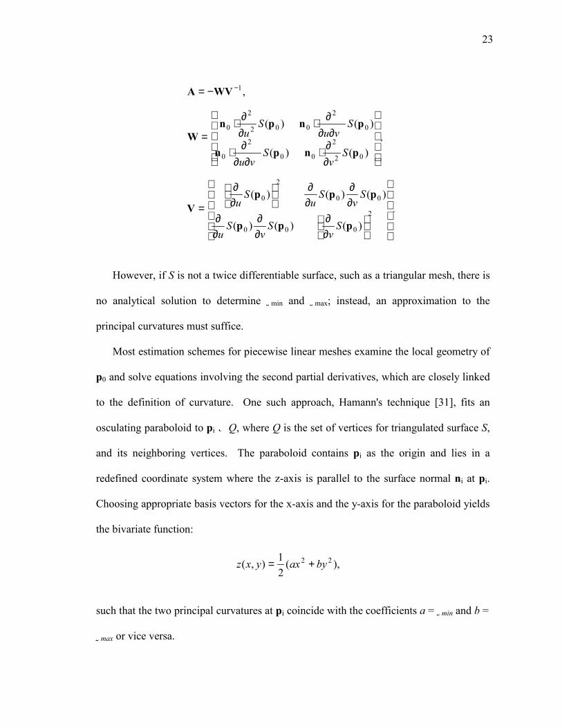
However, if S is not a twice differentiable surface, such as a triangular mesh, there is
no analytical solution to determine â min and â max; instead, an approximation to the
principal curvatures must suffice.
Most estimation schemes for piecewise linear meshes examine the local geometry of
p0 and solve equations involving the second partial derivatives, which are closely linked
to the definition of curvature. One such approach, Hamann's technique [31], fits an
osculating paraboloid to pi Ï Q, where Q is the set of vertices for triangulated surface S,
and its neighboring vertices. The paraboloid contains pi as the origin and lies in a
redefined coordinate system where the z-axis is parallel to the surface normal ni at pi.
Choosing appropriate basis vectors for the x-axis and the y-axis for the paraboloid yields
the bivariate function:
such that the two principal curvatures at pi coincide with the coefficients a = â min and b =
â max or vice versa.
),(21),( 22 byaxyxz +=
. S
vS
vS
u
Sv
Su
Su
,S
vS
vu
Svu
Su
∂∂
∂∂
∂∂
∂∂
∂∂
∂∂
=
∂∂⋅
∂∂∂⋅
∂∂∂⋅
∂∂⋅
=
−= −
2
000
00
2
0
02
2
00
2
0
0
2
002
2
0
1
)()()(
)()()(
)()(
)()(
,
ppp
pppV
pnpn
pnpnW
WVA

24
Thus, the approximation algorithm must construct the osculating paraboloid and
solve the bivariate function. It accomplishes these tasks for each vertex pi of the
triangulated surface S in the following steps:
1. Determine the platelets yj, i.e. the neighboring vertices, associated with pi.
2. Compute the plane P passing through pi and having ni as its normal.
3. Define an orthonormal coordinate system in P with pi as its origin and two
arbitrary unit vectors in P.
4. Compute the distances dj of all platelets from the plane P.
5. Project all platelet points onto the plane P and represent their projections with
respect to the local coordinate system in P.
6. Interpret the projections in P as abscissae values and the vertical distances of
the original platelet from P as ordinate values.
7. Construct a bivariate polynomial f approximating these ordinate values.
8. Compute the principal curvatures of f's graph at pi.
Vector algebra makes Steps 1 through 7 relatively straightforward. Step 8, on the other
hand, is a little more complex. First, it requires a solution to the coefficients c2,0 , c1,1
and c0,2 of the over-determined system of linear equations:
The elements dj for j = 1�n, where n is the number of platelets, in vector d are the
distances from the each platelet to the plane P calculated in step 4. The elements of the
. d
d
ccc
vvuu
vvuu
nnnnn
===
ΜΜΜΜ1
2,0
1,1
0,2
22
2111
21
2
2
21 dUc

25
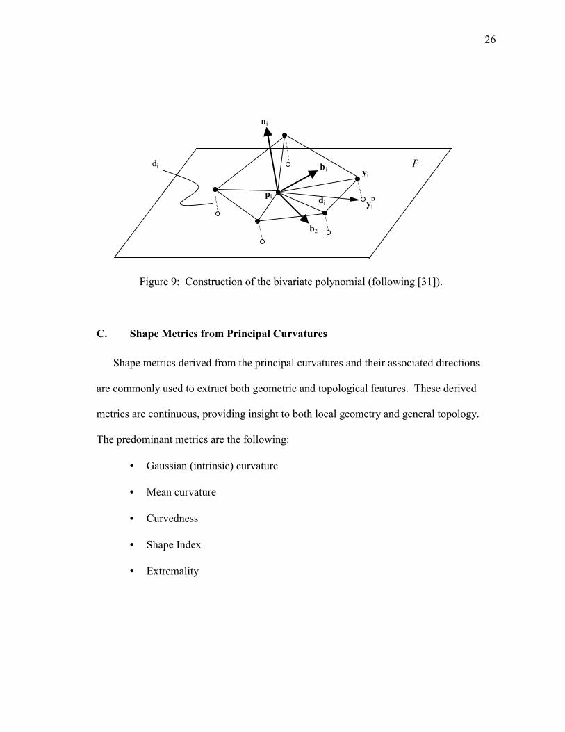
matrix U are defined as uj = dj ıııı b1 and vj = dj ıııı b2 for j = 1�n. The vectors b1 and b2 are
the basis vectors computed in step 3. The difference vector dj is defined by the
following (see Figure 9):
A least squares solution [51] to the normal equation
provides the coefficients c2,0 , c1,1 and c0,2. The final task in step 8 is to compute the real
roots of the quadratic equation
to obtain the estimates for the principal curvatures â min and â max. Then, determining the
principal curvature directions tmin and tmax requires the solution to the following linear
equations:
P. onto projected point platelet a is where
,
,)()(
jPj
0Pjj
22j11jj
yy
pyx
bbxbbxd
−=
⋅+⋅=
dUUcU TT =
0)( 21,12,00,22,00,2 =−++− ccccc ââ O
,minminmin tAt =â==−
. where
,
2,01,1
1,10,2
maxmaxmax
=−
=−
cccc
A
tAt â=
26
C. Shape Metrics from Principal Curvatures
Shape metrics derived from the principal curvatures and their associated directions
are commonly used to extract both geometric and topological features. These derived
metrics are continuous, providing insight to both local geometry and general topology.
The predominant metrics are the following:
• Gaussian (intrinsic) curvature
• Mean curvature
• Curvedness
• Shape Index
• Extremality
ni
b1
b2
yjP
piyj
pdj
dj
Figure 9: Construction of the bivariate polynomial (following [31]).
27
Gaussian curvature (or intrinsic curvature) K is the product of the principal
curvatures; its equation is formulated below.
Gaussian curvature is an intrinsic geometric property; it stays the same no matter how a
surface is bent, as long as it is not distorted, neither stretched nor compressed. The
Gaussian curvature measures how "curved" the surface is at pi. Very curved regions
yield high positive K >> 0 while flat regions yield K ] 0. Saddle regions yield negative
K < 0. In essence, the Gaussian curvature is a continuous metric for the curvature of the
surface.
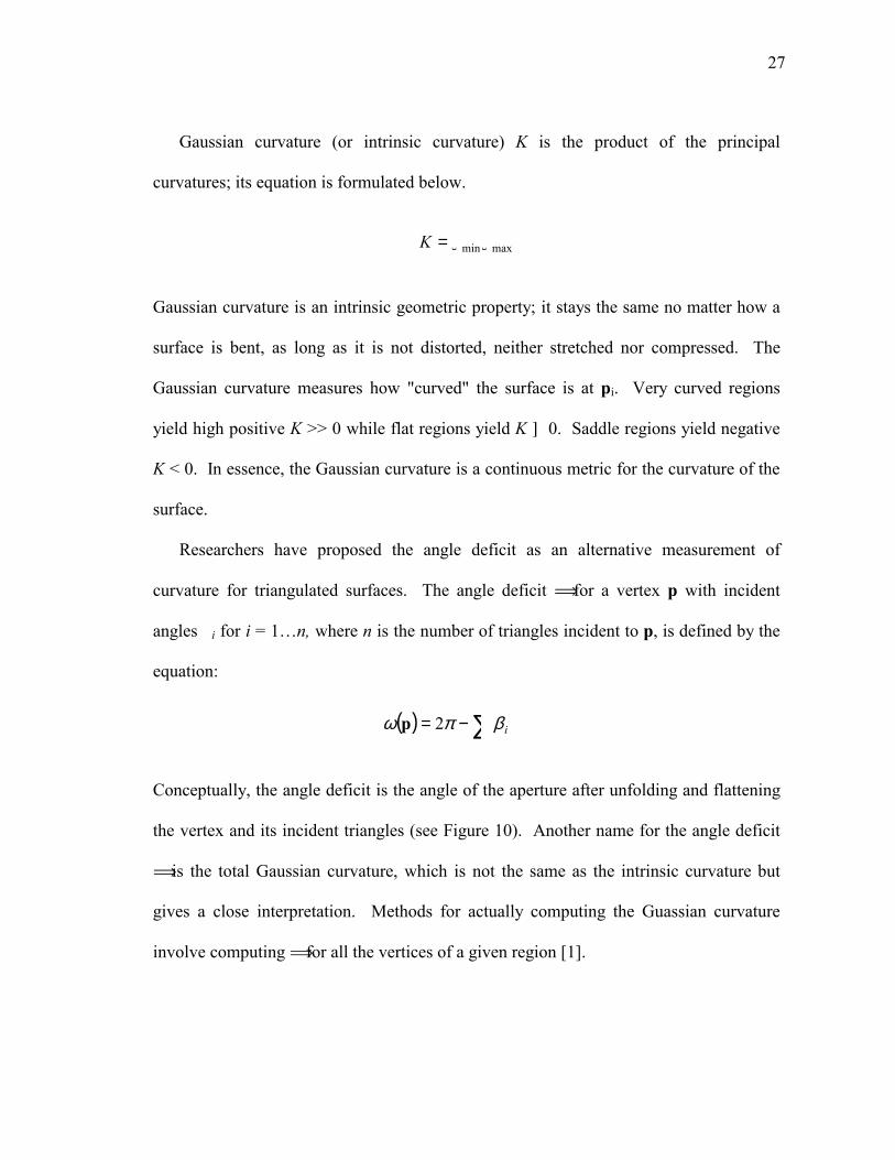
Researchers have proposed the angle deficit as an alternative measurement of
curvature for triangulated surfaces. The angle deficit ï for a vertex p with incident
angles Äi for i = 1�n, where n is the number of triangles incident to p, is defined by the
equation:
Conceptually, the angle deficit is the angle of the aperture after unfolding and flattening
the vertex and its incident triangles (see Figure 10). Another name for the angle deficit
ï is the total Gaussian curvature, which is not the same as the intrinsic curvature but
gives a close interpretation. Methods for actually computing the Guassian curvature
involve computing ï for all the vertices of a given region [1].
( ) ∑−= iβπω 2p
maxmin ââ=K
28
Another common shape metric is the mean curvature H, defined as the average of the
principal curvatures:
The mean curvature tells how inwardly or outwardly a surface region folds. It attains
positive values for concave regions, negative values for convex regions, and near zero
values for flat regions or saddle regions where the principal curvatures cancel each other
out.
Curvedness and shape index are not as widely used as intrinsic and mean curvature,
but their heightened acuity and predictable range of values make them good alternatives.
Curvedness R is defined by the following equation:
. R2
)( 2max
2min ââ +
=
Figure 10: Unfolding a vertex and its incident triangles.
. H2
)( maxmin ââ +=
pi
1
2
ï=
29
As the name suggests, R measures how curved a region is. Flat regions yield R ] 0
while highly curved regions yield large values R. Curvedness is similar to intrinsic
curvature, except it is nonnegative and uninfluenced by the topological region type.
Shape index S is defined by the equation:
The shape index is a generalized measure of concavity and convexity with a range of S =
[-1,1]. It describes the local shape at the surface point pi independent of the scale of the
surface. A convex surface point with equal principal curvatures has a shape index of 1.
A concave surface point with equal principal curvatures has a shape index of -1. A
saddle point with principal curvatures of equal magnitude and opposite sign has a shape
index of 0. A "ridge-like" surface point has a shape index of about 0.5 while a "valley-
like" surface point has a shape index of about -0.5.
Extremality, as defined in [59], is the directional derivative of the principal
curvatures â min and â max in the corresponding principal directions tmin and tmax. The two
extremality functions emin and emax characterizes the extremality at surface point pi; their
formal definitions are the following:
. S
−+
−=maxmin
maxminarctan2ââ
ââ
π
,e minmin minât∇=
. e maxmax maxât∇=
30
Methods based on the extremality functions can extract features such as extremal points
and ridge lines.
D. Topological and Geometric Features
Feature extraction usually focuses on regions of sharp local change or on an object's
global structure. We discuss the extraction of two commonly desired features in
Computer Aided Graphical Design (CAGD) and biomedical imaging: topological
regions and extremal points. These features directly correspond to gyri and sulci,
neuroanatomical structures that characterize the convolutions of the neocortex. As
further discussed in Chapter V, our neocortical finite element decomposition rests on the
identification of these features.
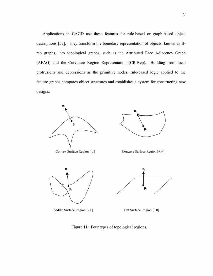
Topological regions are classified into four types: depressions, protrusions, saddles,
and plains. The principal curvatures' sign values [â min, â max] indicate the type of local
topological region in which a point pi on the surface lies.
Table 1: Curvature sign values for the four types of topological regions.
[â min, â max] Topological Region
[+,+] or [+,0] Concave surface region (local depression)
[-,-] or [0,-] Convex surface region (local protrusion)
[+,-] or [-,+] Saddle surface region (local saddle)
[0,0] Flat surface region (local plain)
31
Applications in CAGD use these features for rule-based or graph-based object
descriptions [57]. They transform the boundary representation of objects, known as B-
rep graphs, into topological graphs, such as the Attributed Face Adjacency Graph
(AFAG) and the Curvature Region Representation (CR-Rep). Building from local
protrusions and depressions as the primitive nodes, rule-based logic applied to the
feature graphs compares object structures and establishes a system for constructing new
designs.
pi
ni
pi
Convex Surface Region [-,-]
ni
Concave Surface Region [+,+]
pi
ni
Saddle Surface Region [-,+] Flat Surface Region [0,0]
pi
ni
Figure 11: Four types of topological regions.
32
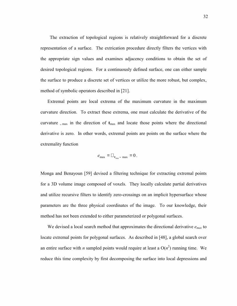
The extraction of topological regions is relatively straightforward for a discrete
representation of a surface. The extrication procedure directly filters the vertices with
the appropriate sign values and examines adjacency conditions to obtain the set of
desired topological regions. For a continuously defined surface, one can either sample
the surface to produce a discrete set of vertices or utilize the more robust, but complex,
method of symbolic operators described in [21].
Extremal points are local extrema of the maximum curvature in the maximum
curvature direction. To extract these extrema, one must calculate the derivative of the
curvature â max in the direction of tmax and locate those points where the directional
derivative is zero. In other words, extremal points are points on the surface where the
extremality function
Monga and Benayoun [59] devised a filtering technique for extracting extremal points
for a 3D volume image composed of voxels. They locally calculate partial derivatives
and utilize recursive filters to identify zero-crossings on an implicit hypersurface whose
parameters are the three physical coordinates of the image. To our knowledge, their
method has not been extended to either parameterized or polygonal surfaces.
We devised a local search method that approximates the directional derivative emax to
locate extremal points for polygonal surfaces. As described in [48], a global search over
an entire surface with n sampled points would require at least a O(n2) running time. We
reduce this time complexity by first decomposing the surface into local depressions and
. e 0maxmax max=∇= ât
33
protrusions. This partitioning is practical because the boundaries of these topological
regions lie on the flattest portion of the surface, where extremal points are nonexistent.
The approximation for emax and the local search is given below.
The derivative of the curvature â max for a point pi on a surface with the principal
curvature direction tmax is
To approximate the derivative, we let â max(pi + ä tmax ) = â max(pi¿ ), where pi
¿ is a point on
the surface closest to the vector pi + ä tmax. For a surface with n sampled points, a
closest distance search for pi¿ in the neighborhood of pi is accurate and fast if n is
relatively small. The partitioning into depressions and protrusions reduces n to the
number of vertices on the local region and, thus, improves the time complexity.
Then, a local search for vertices where emax approximates zero identifies the extremal
points. Although our approximation technique is not as robust as the one proposed in
[59], it is a much simpler and faster algorithm for polygonal surfaces. For the worst
case, i.e. if there is only one topological region on the surface, our algorithm is still
O(n2); however, for m topological regions with equal number of vertices in each one, the
time complexity reduces by a factor of 1/m. Further, the partitioned regions
automatically categorize the extremal points into crest points and valley points. Crest
points are extrema lying on protrusions, while valley points are those lying on
depressions. This classification is particularly important for neocortical surfaces, since
crest and valley points correspond to sharp gyral and sulcal folding.
. )()(
lim )( imaxmaximax0imaxmax max λ
λλ
ptpptââ
â−+
=∇=→
e
34
CHAPTER IV
B-SPLINE TENSOR PATCHES
A. Introduction
Polygonal surface reconstruction methods, including the Delaunay triangulation
technique described in Chapter II, can easily overcome many aspects of surface
reconstruction, namely the tiling and the branching problems, but they share two major
limitations. First, these techniques can only generate a C0 continuous (piecewise linear)
surface represented as a connected set of polygons. Second, the resultant polygonal
mesh requires expensive storage space and computation time for graphical rendering,
especially if interactive navigation is employed. To mitigate space and time complexity,
mesh decimation algorithms reduce the number of vertices and edges, but they do so at
the cost of geometric detail. Further, numerical grid generation, either on the surface or
within the B-rep solid model of the human neocortex, requires a parametric
representation of the surfaces (see Chapter V). Approximation functions, such as B-
Splines, allow direct expressions of the necessary boundary constraints for grid
generation, produce a smoother geometric model, and offer a parsimonious
representation with mathematical functions, rather than an explicit mesh.
Given a dataset for a surface embedded in space, the objective is to determine a
smooth and at least C1 continuous approximation function that "optimally" fits the data
points. B-spline tensor products accomplish this task by mapping a rectangular domain
to 3D Euclidean space, optimized by the least squares error between the dataset and the
35
generated surface. For a smoothing spline, the optimality of the fit is determined by a
compromise between the minimization of least square error and a relaxation (or
smoothness) term. For simple cases, such as those resembling a cylinder, surface fitting
with one tensor product yields desirable results; however, the convoluted surface of the
human neocortex requires a covering by a network of tensor product patches. Various
approaches are available to decompose a surface into a network of patches for surface
fitting on a rectangular domain [34], [33], [44], [20]. For the most part, they divide the
surface into simpler patches for local fitting based on geometric features, such as ridge
lines and corners, or topological features, such as critical points. Either the network of
patches is already C1 continuous at incident edges, or they are sown together with a
blending function to ensure C1 continuity at incident edges between patches.
As applied to the human neocortex, we first decompose the tissue into its major gyri
along major sulcal lines and then further divide the cortical folds into patches where
geometric complexity necessitates it. Our mapped template approach is related to the
finite element decomposition technique and is further discussed in Chapter V.
B. B-spline Tensor Product
Spline functions have many applications in numerical analysis and computer aided
geometric design (CAGD). They have proven especially effective in interpolation, data
fitting, data smoothing, and geometric modeling. A spline is a continuous
approximation function for a set of data points R in ����n, where n is the dimension of the
points. Though splines can be extended to arbitrarily high dimensions, geometric
modeling is mainly concerned with datasets in 3D Euclidean space ����3. Tensor product

36
splines, a simple type of bivariate (parameterized in two variables) spline, is a natural
parametric representation of a surface. A B-spline tensor product is a tensor spline that
utilizes the B-spline basis functions as the interpolating polynomials.
The tensor spline s(u,v) of degree k in the u direction and degree l in the v direction
over a rectangular domain D = [a,b] “ [c,d], where a ¡ u ¡ b and c ¡ v ¡ d, for the knot
vector ääää in the u direction and the knot vector ãããã in the v direction, where
is given by the following equation [16]:
The polynomial functions Ni,k+1(u) of degree k and Mj,l+1(v) of degree l are called the B-
spline basis functions, and they are defined as the following:
The tensor spline s(u,v) exhibits many desirable qualities; one of which, useful for
feature extraction, is that all its partial derivatives for 0 ¡ q < k and 0 ¡ p < l are
,110 ba gg =<<<<= +λλλλ Κ,110 dc hh =<<<<= +µµµµ Κ
( ) ( ) ( ). , 1,1,, vMuNcvus lj
g
ki
h
ljkiji +
−= −=+∑ ∑=
( ) ( ) ( )
( ) ( ) ( )
( ) ( ) ( )xtxtxtxtxtg
vtgvM
utguN
mm
m
lliiltililj
kkiiktikiki
<≥
−=−=
∆−=
∆−=
+
+++
+++
+++
+++
if if
0: where
,:,,)(
,:,,)(
11
11,
11
11,
µµµµ
λλλλ
Κ
Κ

37
continuous on R. The partial derivatives can be directly computed with the following
recurrence relation:
Thus, the B-spline tensor product yields a Cmin(k,l) - 1 continuous surface shaped by the
coefficients ci,j and the knot vectors ääää and ãããã.
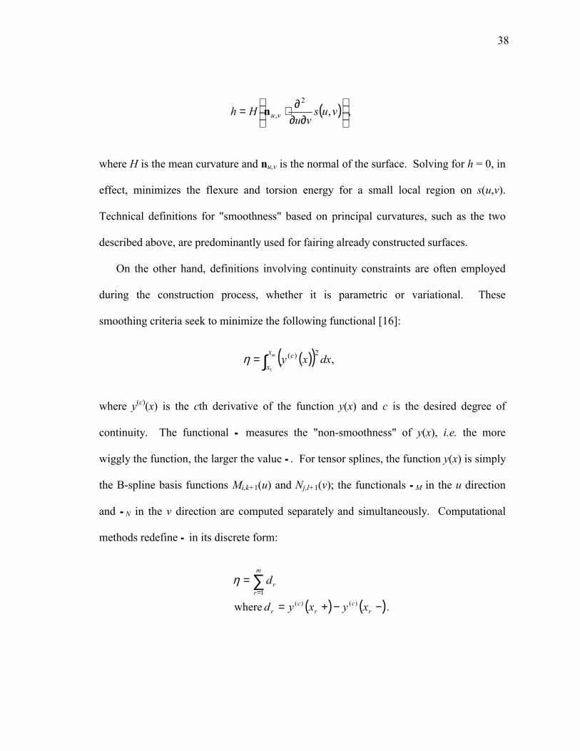
C. Smoothing Criterion
The technical criterion for the "smoothness" or "fairness" of a surface has taken
various forms depending on the desired end results, whether it is a reflectively smooth
surface or a surface with a predefined continuity. Nonetheless, most smoothing criteria
involve the principal curvatures or the differentiability of a surface.
The standard fairness criterion in engineering is given by the following functional
[49]:
It measures the strain energy of flexure and torsion in a thin rectangular elastic plate with
small deflection. Minimizing Ü is analogous to minimizing the curvedness (see Chapter
III), thus producing a "least curved and twisted" surface. Farin and others have extended
the functional Ü to a local twist estimator h(s(u,v)) for tensor splines [23]:
. )( )(),( )(1,
)(1,,∑ ∑
−=+
−=+
+=
∂∂∂ g
ki
qlj
h
lj
pkijiqp
qpvMuNc
vuvus
( ) . s 2max
2min d
s∫ += κκη
38
where H is the mean curvature and nu,v is the normal of the surface. Solving for h = 0, in
effect, minimizes the flexure and torsion energy for a small local region on s(u,v).
Technical definitions for "smoothness" based on principal curvatures, such as the two
described above, are predominantly used for fairing already constructed surfaces.
On the other hand, definitions involving continuity constraints are often employed
during the construction process, whether it is parametric or variational. These
smoothing criteria seek to minimize the following functional [16]:
where y(c)(x) is the cth derivative of the function y(x) and c is the desired degree of
continuity. The functional Ü measures the "non-smoothness" of y(x), i.e. the more
wiggly the function, the larger the value Ü . For tensor splines, the function y(x) is simply
the B-spline basis functions Mi,k+1(u) and Nj,l+1(v); the functionals ÜM in the u direction
and Ü N in the v direction are computed separately and simultaneously. Computational
methods redefine Ü in its discrete form:
( ) , ,2
,
∂∂
∂⋅= vusvu
Hh vun
( )( ) ,1
2)(∫= mx
xc dxxyη
( ) ( ). where )()(1
−−+=
= ∑=
rc
rc
r
m
rr
xyxyd
dη

39
The metric dr, the difference between the cth derivatives from the left and right
directions, measures the discontinuity jumps between neighboring points. Dierckx's
algorithm for smooth surface fitting, as described in the next section, utilizes this
discrete form of Ü to compromise smoothness with the closeness of fit. Others, such as
[30], have extended the functional Ü to a variational calculus approach for surface fitting
to a set of scattered sample points.
D. Smooth Surface Fitting over a Rectangular Domain
B-spline tensor products are often used in CAGD to model a surface defined by the
sample data points R either as a scattered dataset or as a grid in parameter space defined
by a rectangle, a cylinder, a sphere, or another simple geometric construct. Surface
fitting over a grid can be interpreted as mapping a simple geometric object, such as a
cylinder, into the surface defined over R. We restrict our discussion to surface fitting
over a rectangular grid because of its simplicity and popularity, but, most important of
all, the rectangular mesh maps easily to one of the six faces of a hexahedral finite
element. For a thorough discussion of surface fitting using B-splines, refer to [16].
Given sample data points Rq,r in ����3 defined over a rectangular grid with points
(uq,vr), where q = 1�n and r = 1�m, the surface fitting problem is to find a B-spline
tensor approximation s(u,v) minimizing an optimality constraint. In particular, a
smoothing B-spline tensor sp(u,v) compromises the closeness of fit with smoothness for
an optimal approximation. The bias between the two constraints is controlled by a
smoothing parameter p. As pà 0, the approximation function sp tends toward a weighted

40
least squares polynomial (smoothest fit ); on the other hand, as pÃ√ , sp tends toward the
natural interpolating spline (closest fit).
Fitting the surface defined by Rq,r requires the determination of the B-spline
coefficients ci,j, the knot vectors ääää and ãããã, and the smoothing parameter p which satisfies
the solution to the smoothing function F(p) = S, where S is the target error for the
following least squares equation:
Dierckx has implemented an iterative method for determining the parameters ci,j, ääää, ãããã,
and p given a target error value S [16]. The bivariate smoothing spline function s0(u,v) is
solved by computing the least squares solution for the B-spline coefficients ci,j to the
following equations
( )( ) SvusRpFn
q
m
rrqprq =−= ∑∑
= =
2
1 1, ,)(
( ) ( )
( )
( )
....1 ,...1 ,01
...1 ,...1 ,0 1
....1 ,...1 ,0 1
....1 ,...1 ,
,,,
,,1,
,,1,
,,1,1,
hrgqcbap
mrgqcavMp
hrnqcbuNp
mrnqRcvMuN
jirj
g
ki
h
ljqi
ji
g
ki
h
ljqirlj
jirj
g
ki
h
ljqki
rqjirlj
g
ki
h
ljqki
===
===
===
===
∑ ∑
∑ ∑
∑ ∑
∑ ∑
−= −=
−= −=+
−= −=+
+−= −=
+
41
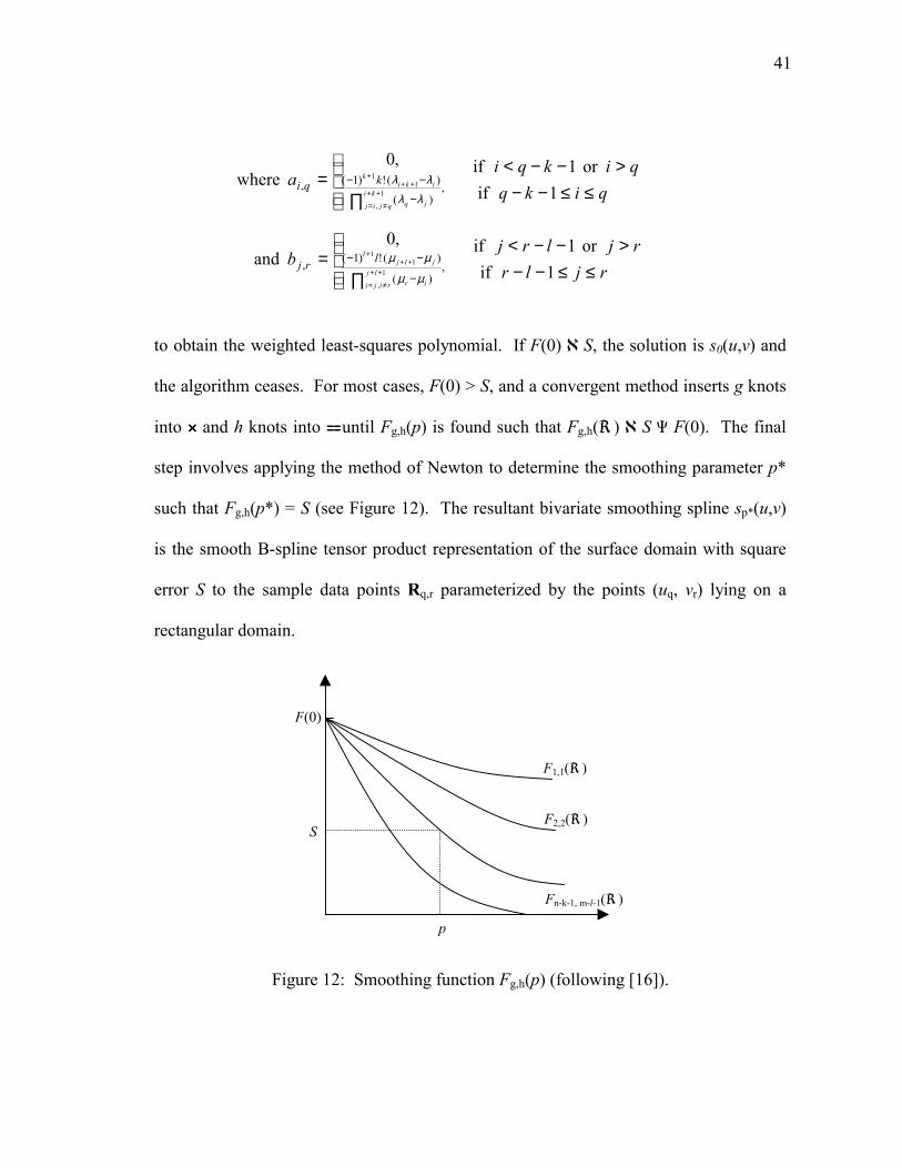
to obtain the weighted least-squares polynomial. If F(0) ¡ S, the solution is s0(u,v) and
the algorithm ceases. For most cases, F(0) > S, and a convergent method inserts g knots
into ääää and h knots into ãããã until Fg,h(p) is found such that Fg,h(√ ) ¡ S Y F(0). The final
step involves applying the method of Newton to determine the smoothing parameter p*
such that Fg,h(p*) = S (see Figure 12). The resultant bivariate smoothing spline sp*(u,v)
is the smooth B-spline tensor product representation of the surface domain with square
error S to the sample data points Rq,r parameterized by the points (uq, vr) lying on a
rectangular domain.
F(0)
F1,1(√ )
F2,2(√ )
Fn-k-1, m-l-1(√ )
S
p
Figure 12: Smoothing function Fg,h(p) (following [16]).
≤≤−−>−−<
∏=
≤≤−−>−−<
∏=
++
≠=
+++
++
≠=
+++
−
−−
−
−−
rjlrrjlrj
b
qikqqikqi
a
lj
riji ir
jljl
ki
qjij jq
ikik
lrj
kqi
1 ifor 1 if ,0
and
1 ifor 1 if ,0
where
,)(
)( !)1(,
,)(
)( !)1(,
1
,
11
1
,
11
µµ
µµ
λλλλ
42
Because the least square error threshold S is an absolute term without regards for
either the distribution or the physical dimensions of the sample data, choosing the same
S value for two different data sets can yield two surfaces with dramatically varying
smoothness. To exercise more control over the smoothness of sp(u,v) for arbitrary
datasets, we define the smoothing factor S´ relative to the approximate surface area AR of
Rq,r as the following:
For S´ ¡ 0.01, the B-spline tensor product resembles the natural interpolating spline (the
least smooth approximation), and for S´ — 100, the tensor product resembles the
weighted least squares polynomial (the smoothest approximation).
E. Blending B-spline Tensor Product Patches
Surface modeling of convoluted free-form surfaces, e.g. the exterior surface of the
human neocortex, requires a collection of surface patches, each capturing the geometry
for simpler local regions. The continuity of each tensor patch can be controlled with the
degree of the basis functions. However, if the patches are constructed separately,
nothing guarantees the continuity between the edges of the patches. Adjacent patch
boundaries may not even meet, much less differentiable at incident edges.
( ) ( )∑∑−
=
−
=++ −×−=
=′
1
1
1
111
n
q
m
rqqqqR
R
A
ASS
yyxx
43
A covering of patches is termed GCn continuous if it is n times differentiable on both
the patches and the boundaries between them. The objective of most CAGD
applications, and our surface modeling of the neocortex, aims to construct a GC1
continuous covering. Because cubic B-spline tensor products already guarantee C2
continuity on individual patches, the remaining task is to enforce C1 continuity across
patch boundaries. To achieve GC1, a blending surface smoothly connects the patch
boundaries, "stitching" the patch network together.
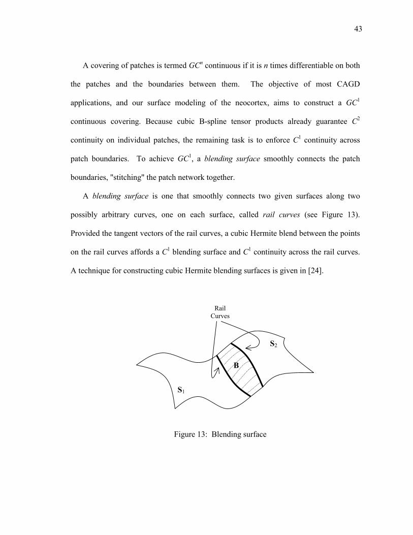
A blending surface is one that smoothly connects two given surfaces along two
possibly arbitrary curves, one on each surface, called rail curves (see Figure 13).
Provided the tangent vectors of the rail curves, a cubic Hermite blend between the points
on the rail curves affords a C1 blending surface and C1 continuity across the rail curves.
A technique for constructing cubic Hermite blending surfaces is given in [24].
S1
S2
B
Rail Curves
Figure 13: Blending surface

44
Let S1(u1,v1) and S2(u2,v2) be the base surfaces to blend and c1(t) and c2(t) be the rail
curves in the parameter space of S1 and S2, where ci(t) = (ui(t), vi(t)), i = 1, 2. The two
rail curves C1(t) and C2(t) on the base surfaces are then
Also, let T1(t) and T2(t) be the tangent vectors on S1 and S2 along the two rail curves.
The blending surface B(s,t) of S1(u1,v1) and S2(u2,v2) is then given by the cubic Hermite
blending:
Choosing the boundary curves of the patches as the rail curves, which are precisely the
iso-u and iso-v curves at u = 0, u = 1, v = 0, and v = 1, a GC1 surface is constructed from
a network of B-spline tensor patches.
( ) ( )( ) .2,1 , == itt iii cSC
( ) ( ) ( ) ( ) ( ) ( ) ( ) ( ) ( )
( ) ( )( ) ( )
( ) ( )
( ) ( ) . sssH
sssH
sHsH
sssH
tsHtsHtsHtsHts
1
,1
,1
,132
,,
24
23
12
21
24132211
−=
−=
−=
+−=
+++= TTCCB
45
CHAPTER V
OVERVIEW OF NEOCORTICAL FINITE ELEMENT DECOMPOSITION
A. Introduction to Finite Element Mesh Generation
Finite element mesh generation is the process of decomposing a geometric object
into simpler finite elements (FE's), usually defined as triangles or quadrilaterals in two-
dimensional geometry, and tetrahedrons and hexahedrons in three-dimensional
geometry. Various engineering disciplines and CAGD have made significant advances
in FE mesh generation for surfaces (2D manifolds in 3D space), but the problem
extended to volume FE's still remains an imposing and laborious task [55]. Most current
methods only take into account the local geometry of the object, without consideration
for other predefined constraints. Predominant automated techniques include the
advancing front method [41], [42], plastering [6], paving [7], [15], and the point-based
approach [40]. These methods iteratively lay down subsets of finite elements until the
entire mesh is generated. At each iteration and at the conclusion of mesh construction,
they apply topological and geometric operators to further optimize the mesh. A related
problem in texture mapping is to map a structured grid onto the surface of a 3D object
[44]. This research has predicated interactive techniques that partition the surface into
regions under feature-based constraints. In short, laying a mesh on an arbitrary free-
form geometric object continues to be an area of prolific research. All methods differ in
46
their definition of optimality, but a quality desired by almost all applications is the
generated mesh that closely resembles a structured grid.
Finite element mesh generation provides a framework for the spatial management,
analysis, and visualization of complex geometric objects. Applied to the human
neocortex, the decomposition of the cortical shells into hexahedral finite elements
provides a structural information framework for the human brain and scaffolding for the
implantation of oriented neurons. The neocortical finite elements should satisfy
neuroanatomical consistency, a set of constraints based on the features of the cortical
tissue, in addition to the traditional constraints of FE meshes. Before describing the
mapped template method used in this thesis, neuroanatomical consistency and the
neocortical finite element decomposition problem are formulated below.
B. The Neocortical Finite Element Decomposition Problem
The objective is to generate a 3D finite element mesh over the human neocortex that
provides the following:
(1) A structural information framework for the human neocortex
(2) Finite elements for the 3D graphical mapping of neurons
(3) Finite elements of simple geometry
Formulating the constraints for the generation of this FE mesh requires the consideration
for (1) the shape and size of each FE, (2) the representation of an individual FE, (3) the
arrangement of the FE's on the mesh, and (4) the organizational complexity of the mesh.
We first discuss the four constraints, and then we redefine the neocortical finite element
decomposition problem in more formal terms.
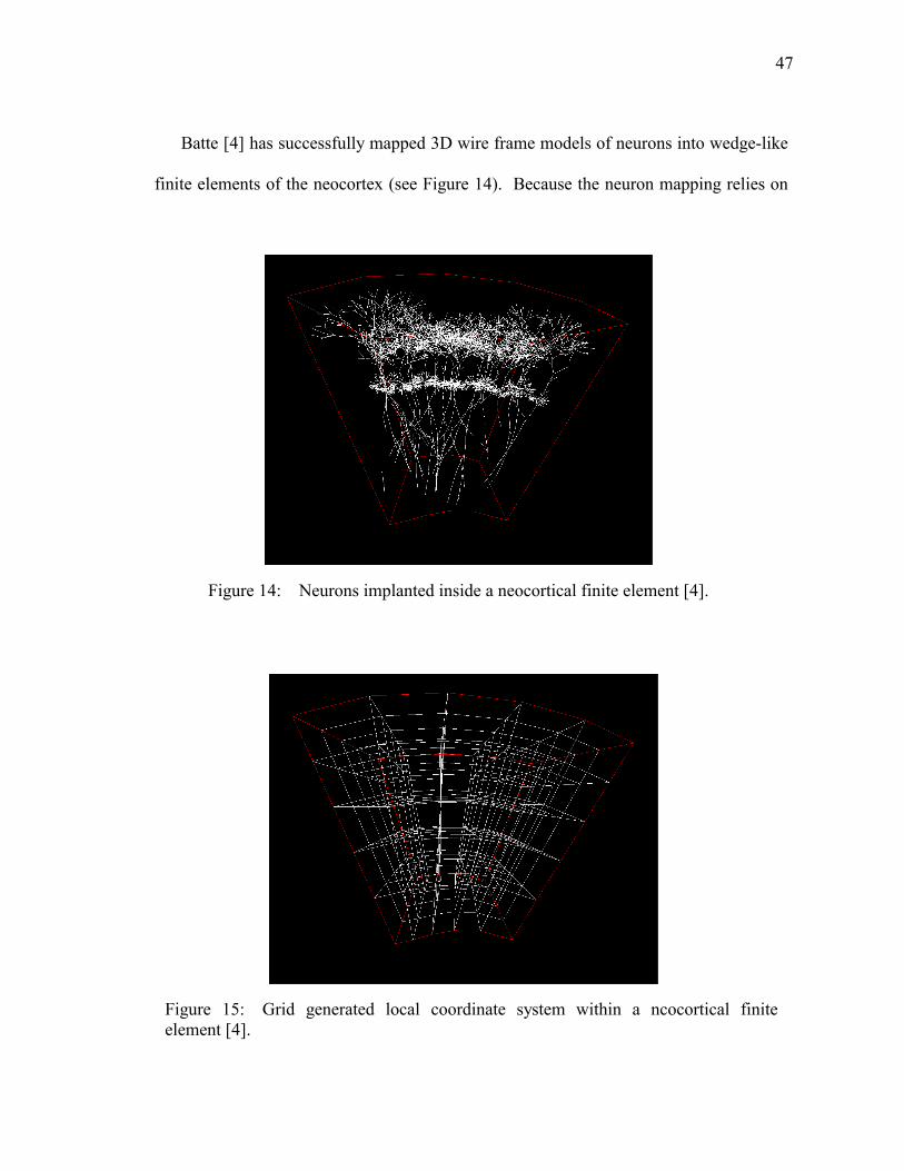
47
Batte [4] has successfully mapped 3D wire frame models of neurons into wedge-like
finite elements of the neocortex (see Figure 14). Because the neuron mapping relies on
Figure 14:15Neurons implanted inside a neocortical finite element [4].
Figure 15:14Grid generated local coordinate system within a ncocortical finiteelement [4].
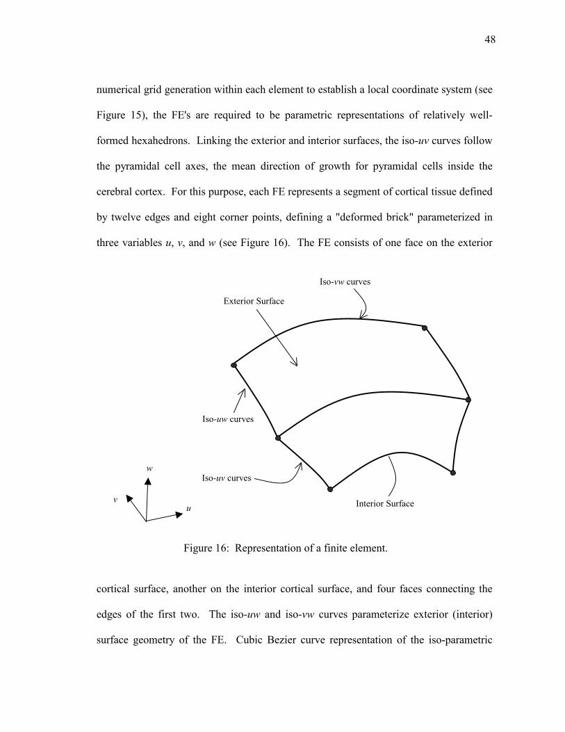
48
numerical grid generation within each element to establish a local coordinate system (see
Figure 15), the FE's are required to be parametric representations of relatively well-
formed hexahedrons. Linking the exterior and interior surfaces, the iso-uv curves follow
the pyramidal cell axes, the mean direction of growth for pyramidal cells inside the
cerebral cortex. For this purpose, each FE represents a segment of cortical tissue defined
by twelve edges and eight corner points, defining a "deformed brick" parameterized in
three variables u, v, and w (see Figure 16). The FE consists of one face on the exterior
cortical surface, another on the interior cortical surface, and four faces connecting the
edges of the first two. The iso-uw and iso-vw curves parameterize exterior (interior)
surface geometry of the FE. Cubic Bezier curve representation of the iso-parametric
Figure 16: Representation of a finite element.
w
v u Interior Surface
Exterior Surface
Iso-vw curves
Iso-uw curves
Iso-uv curves
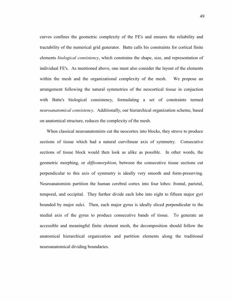
49
curves confines the geometric complexity of the FE's and ensures the reliability and
tractability of the numerical grid generator. Batte calls his constraints for cortical finite
elements biological consistency, which constrains the shape, size, and representation of
individual FE's. As mentioned above, one must also consider the layout of the elements
within the mesh and the organizational complexity of the mesh. We propose an
arrangement following the natural symmetries of the neocortical tissue in conjuction
with Batte's biological consistency, formulating a set of constraints termed
neuroanatomical consistency. Additionally, our hierarchical organization scheme, based
on anatomical structure, reduces the complexity of the mesh.
When classical neuroanatomists cut the neocortex into blocks, they strove to produce
sections of tissue which had a natural curvilinear axis of symmetry. Consecutive
sections of tissue block would then look as alike as possible. In other words, the
geometric morphing, or diffeomorphism, between the consecutive tissue sections cut
perpendicular to this axis of symmetry is ideally very smooth and form-preserving.
Neuroanatomists partition the human cerebral cortex into four lobes: frontal, parietal,
temporal, and occipital. They further divide each lobe into eight to fifteen major gyri
bounded by major sulci. Then, each major gyrus is ideally sliced perpendicular to the
medial axis of the gyrus to produce consecutive bands of tissue. To generate an
accessible and meaningful finite element mesh, the decomposition should follow the
anatomical hierarchical organization and partition elements along the traditional
neuroanatomical dividing boundaries.
50
The finite element mesh should therefore conform to three types of neuroanatomical
boundaries. First, deep sulcal folds that partition the neocortex into major anatomical
gyri intuitively establish curvilinear dividing boundaries for sets of finite elements.
These dividing borders are called major sulcal boundaries. Second, the line of
symmetry along the center of the top of a gyrus, splitting it into ventral and dorsal
slopes, provides another partitioning constraint for the elements. These lines are called
gyral lines of symmetry. Third, neuroanatomists cut perpendicular to the medial axis of
a gyrus to extract tissue segments resembling ribs. These guiding cutting planes are
called gyral ribs. Thus, the notion of neuroanatomical consistency incorporates the
three types of dividing boundaries (see Figure 17).
We now pose the following mesh generation problem as the neocortical finite
element decomposition problem:
{ }
( ) ( )
G withconsistentmically neuroanato is ) v (
G to rlly similageometrica is ) iv (
G withcompatiblelly topologica is ) iii
sinteriorsinterior ,ji each For ) ii (
G s each in points the All ) i (
:properties following the satisfy setthe of members The element.
hexahedral thi the is s wheressss iondecomposit
hexahedralthefindGneocortextheoftionrepresenta geometric a Given
ji
i
iN
Λ
Λ
Λ
=∩≠
∈
Λ
=Λ
(
0
,,,,,
,
321 Κ
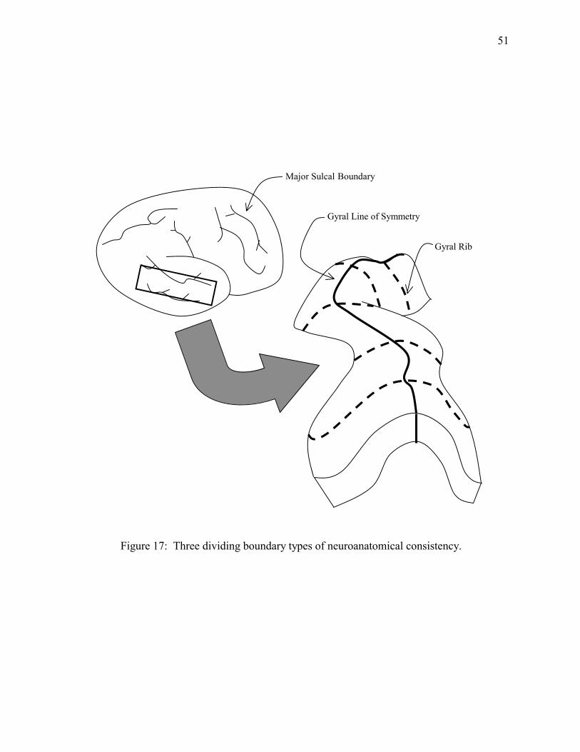
51
Figure 17: Three dividing boundary types of neuroanatomical consistency.
Major Sulcal Boundary
Gyral Rib
Gyral Line of Symmetry
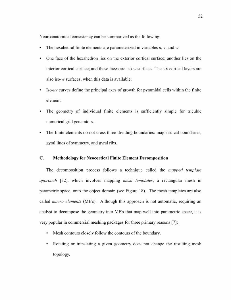
52
Neuroanatomical consistency can be summarized as the following:
• The hexahedral finite elements are parameterized in variables u, v, and w.
• One face of the hexahedron lies on the exterior cortical surface; another lies on the
interior cortical surface; and these faces are iso-w surfaces. The six cortical layers are
also iso-w surfaces, when this data is available.
• Iso-uv curves define the principal axes of growth for pyramidal cells within the finite
element.
• The geometry of individual finite elements is sufficiently simple for tricubic
numerical grid generators.
• The finite elements do not cross three dividing boundaries: major sulcal boundaries,
gyral lines of symmetry, and gyral ribs.
C. Methodology for Neocortical Finite Element Decomposition
The decomposition process follows a technique called the mapped template
approach [32], which involves mapping mesh templates, a rectangular mesh in
parametric space, onto the object domain (see Figure 18). The mesh templates are also
called macro elements (ME's). Although this approach is not automatic, requiring an
analyst to decompose the geometry into ME's that map well into parametric space, it is
very popular in commercial meshing packages for three primary reasons [7]:
• Mesh contours closely follow the contours of the boundary.
• Rotating or translating a given geometry does not change the resulting mesh
topology.
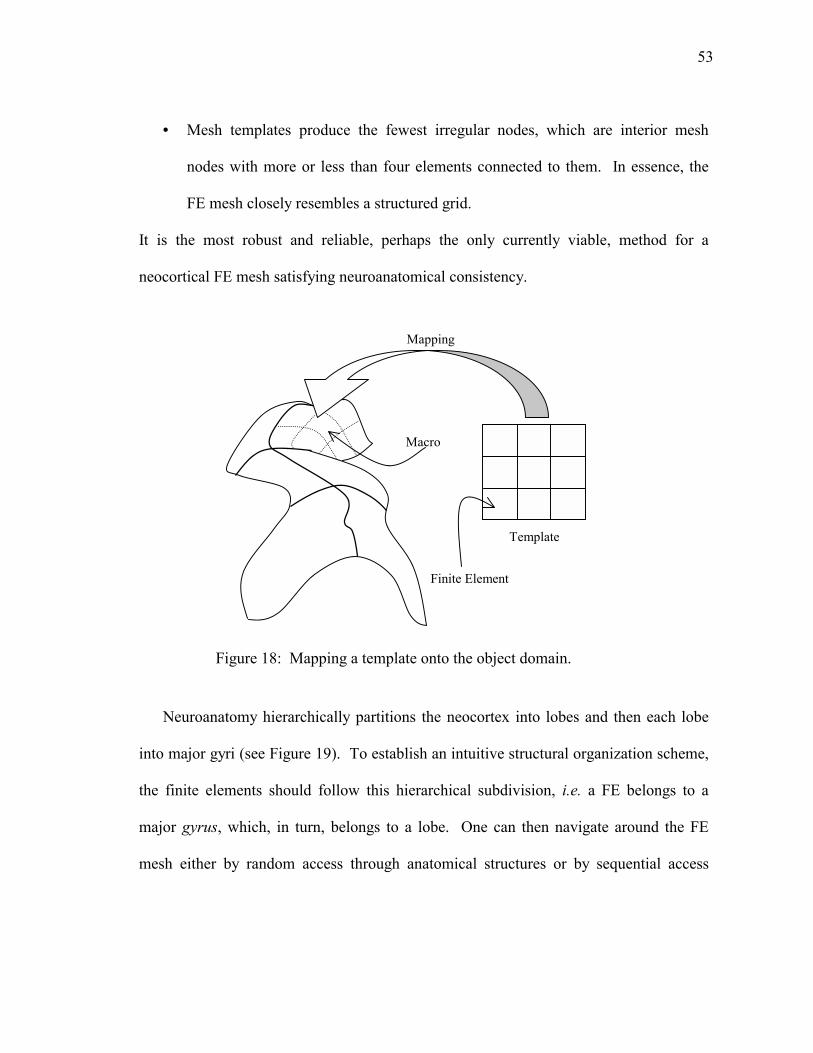
53
• Mesh templates produce the fewest irregular nodes, which are interior mesh
nodes with more or less than four elements connected to them. In essence, the
FE mesh closely resembles a structured grid.
It is the most robust and reliable, perhaps the only currently viable, method for a
neocortical FE mesh satisfying neuroanatomical consistency.
Neuroanatomy hierarchically partitions the neocortex into lobes and then each lobe
into major gyri (see Figure 19). To establish an intuitive structural organization scheme,
the finite elements should follow this hierarchical subdivision, i.e. a FE belongs to a
major gyrus, which, in turn, belongs to a lobe. One can then navigate around the FE
mesh either by random access through anatomical structures or by sequential access
Figure 18: Mapping a template onto the object domain.
Template
Mapping
Macro
Finite Element
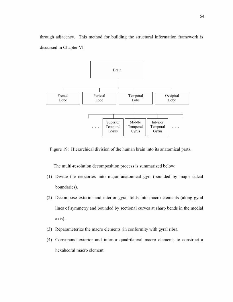
54
through adjacency. This method for building the structural information framework is
discussed in Chapter VI.
The multi-resolution decomposition process is summarized below:
(1) Divide the neocortex into major anatomical gyri (bounded by major sulcal
boundaries).
(2) Decompose exterior and interior gyral folds into macro elements (along gyral
lines of symmetry and bounded by sectional curves at sharp bends in the medial
axis).
(3) Reparameterize the macro elements (in conformity with gyral ribs).
(4) Correspond exterior and interior quadrilateral macro elements to construct a
hexahedral macro element.
Brain
Frontal Lobe
Occipital Lobe
Temporal Lobe
Parietal Lobe
Inferior Temporal
Gyrus
Middle Temporal
Gyrus
SuperiorTemporal
Gyrus . . . . . .
Figure 19: Hierarchical division of the human brain into its anatomical parts.
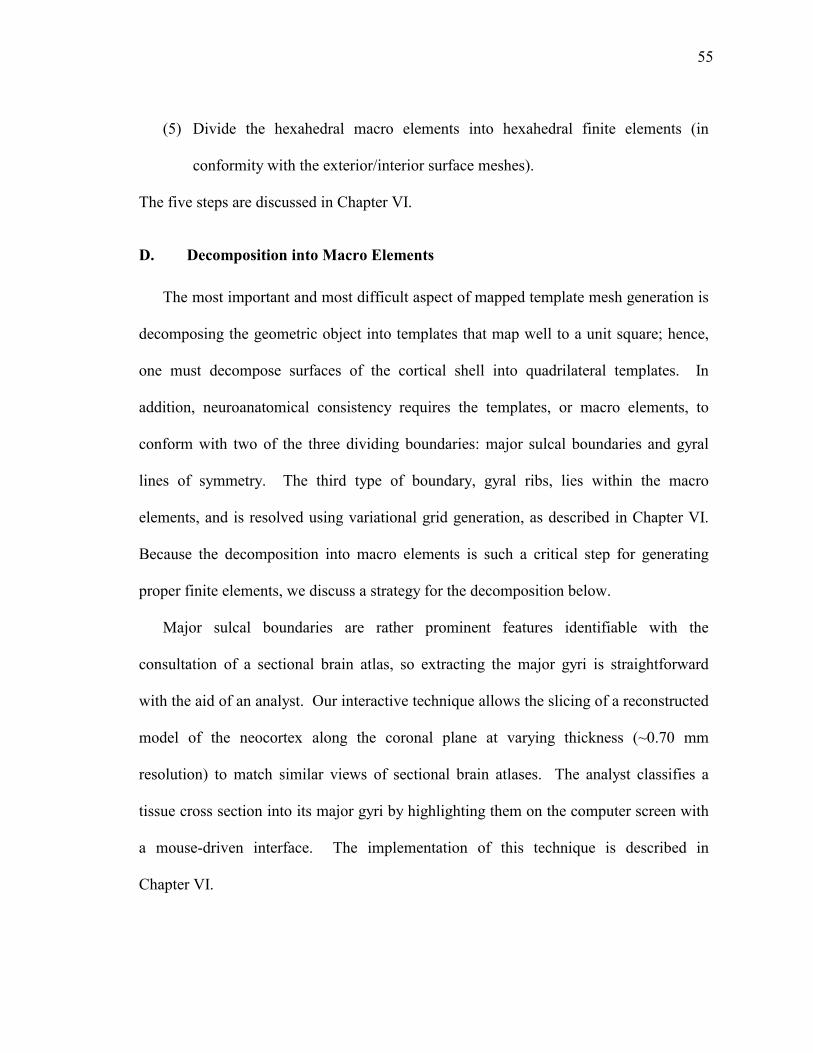
55
(5) Divide the hexahedral macro elements into hexahedral finite elements (in
conformity with the exterior/interior surface meshes).
The five steps are discussed in Chapter VI.
D. Decomposition into Macro Elements
The most important and most difficult aspect of mapped template mesh generation is
decomposing the geometric object into templates that map well to a unit square; hence,
one must decompose surfaces of the cortical shell into quadrilateral templates. In
addition, neuroanatomical consistency requires the templates, or macro elements, to
conform with two of the three dividing boundaries: major sulcal boundaries and gyral
lines of symmetry. The third type of boundary, gyral ribs, lies within the macro
elements, and is resolved using variational grid generation, as described in Chapter VI.
Because the decomposition into macro elements is such a critical step for generating
proper finite elements, we discuss a strategy for the decomposition below.
Major sulcal boundaries are rather prominent features identifiable with the
consultation of a sectional brain atlas, so extracting the major gyri is straightforward
with the aid of an analyst. Our interactive technique allows the slicing of a reconstructed
model of the neocortex along the coronal plane at varying thickness (~0.70 mm
resolution) to match similar views of sectional brain atlases. The analyst classifies a
tissue cross section into its major gyri by highlighting them on the computer screen with
a mouse-driven interface. The implementation of this technique is described in
Chapter VI.
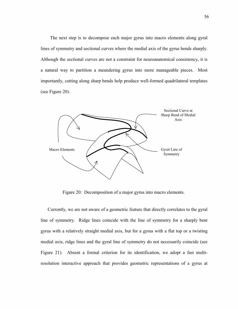
56
The next step is to decompose each major gyrus into macro elements along gyral
lines of symmetry and sectional curves where the medial axis of the gyrus bends sharply.
Although the sectional curves are not a constraint for neuroanatomical consistency, it is
a natural way to partition a meandering gyrus into more manageable pieces. Most
importantly, cutting along sharp bends help produce well-formed quadrilateral templates
(see Figure 20).
Currently, we are not aware of a geometric feature that directly correlates to the gyral
line of symmetry. Ridge lines coincide with the line of symmetry for a sharply bent
gyrus with a relatively straight medial axis, but for a gyrus with a flat top or a twisting
medial axis, ridge lines and the gyral line of symmetry do not necessarily coincide (see
Figure 21). Absent a formal criterion for its identification, we adopt a fast multi-
resolution interactive approach that provides geometric representations of a gyrus at
Macro Elements
Sectional Curve at Sharp Bend of Medial
Axis
Gyral Line of Symmetry
Figure 20: Decomposition of a major gyrus into macro elements.
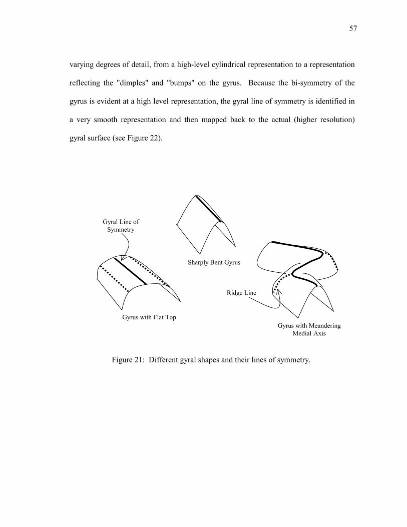
57
varying degrees of detail, from a high-level cylindrical representation to a representation
reflecting the "dimples" and "bumps" on the gyrus. Because the bi-symmetry of the
gyrus is evident at a high level representation, the gyral line of symmetry is identified in
a very smooth representation and then mapped back to the actual (higher resolution)
gyral surface (see Figure 22).
Sharply Bent Gyrus
Gyrus with Flat Top Gyrus with Meandering
Medial Axis
Ridge Line
Gyral Line of Symmetry
Figure 21: Different gyral shapes and their lines of symmetry.
58
High-level Representation of Gyral Surface
Actual Geometry of Gyral Surface
Gyral Line of Symmetry
Figure 22: Mapping gyral line of symmetry at different levels of detail.
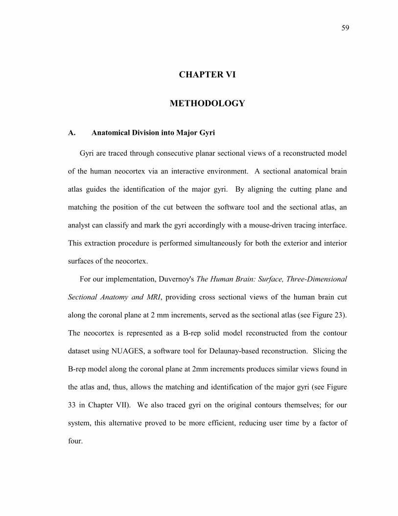
59
CHAPTER VI
METHODOLOGY
A. Anatomical Division into Major Gyri
Gyri are traced through consecutive planar sectional views of a reconstructed model
of the human neocortex via an interactive environment. A sectional anatomical brain
atlas guides the identification of the major gyri. By aligning the cutting plane and
matching the position of the cut between the software tool and the sectional atlas, an
analyst can classify and mark the gyri accordingly with a mouse-driven tracing interface.
This extraction procedure is performed simultaneously for both the exterior and interior
surfaces of the neocortex.
For our implementation, Duvernoy's The Human Brain: Surface, Three-Dimensional
Sectional Anatomy and MRI, providing cross sectional views of the human brain cut
along the coronal plane at 2 mm increments, served as the sectional atlas (see Figure 23).
The neocortex is represented as a B-rep solid model reconstructed from the contour
dataset using NUAGES, a software tool for Delaunay-based reconstruction. Slicing the
B-rep model along the coronal plane at 2mm increments produces similar views found in
the atlas and, thus, allows the matching and identification of the major gyri (see Figure
33 in Chapter VII). We also traced gyri on the original contours themselves; for our
system, this alternative proved to be more efficient, reducing user time by a factor of
four.
60
B. Decomposition of Gyral Folds into Macro Elements
As discussed in Chapter V, the macro elements are divided along the gyral lines of
symmetry and sectional curves at sharp bends of the medial axis of the gyrus. We adopt
a fast, multi-resolution, interactive approach to identify the gyral line of symmetry.
Sectional curves at sharp changes in the medial axis are determined by visual inspection
Figure 23: Sectional view in a human brain atlas.
61
and marked interactively. This procedure applies to both the exterior and interior gyral
surfaces.
A multi-resolution approach, controlled by the smoothness of fit, is employed to
locate the dividing boundaries of the macro elements. The resolution of detail is
controlled by the smoothing factor S´ defined in chapter IV. For the smooth
representation, S´ ] 100, and for the detailed representation, S´ ] 0.01.
First, a very smooth tensor spline is fitted to the gyrus to obtain a high-level
geometric representation that closely resembles a half-tube running along the primary
direction of the medial axis. This smooth approximation filters the noise from small
local variations, dimples and bumps on the surface, to access the global geometry of the
gyrus. Second, an analyst then interactively marks the line of symmetry by identifying
the curve that splits the half-tube into two nearly symmetric slopes. Third, the curve
from the smooth approximation is mapped to a non-smooth tensor spline fitted to the
gyrus. The curve now coincides with the gyral line of symmetry of the actual geometry
of the gyrus. The robustness of the multi-resolution technique requires that the
parameter space warps relatively uniformly from the smooth fit to the close fit. Dividing
the gyrus at sectional curves where the medial axis sharply turns meets this condition.
After the macro element decomposition, we map a unit square in parameter space to
each quadrilateral macro element using the surface fitting algorithms discussed in [16].
The exterior and interior surfaces of the gyrus are now represented as B-spline surface
patches. The decomposition, thus far, has placed no constraints on the parameterization
of the macro element.
62
C. Reparameterization of Macro Elements
Because a regular grid over a macro element (mapped template) defines finite
element boundaries, they must coincide with gyral ribs to ensure the third type of
boundary conformity. Unlike the gyral line of symmetry, gyral ribs have a direct
correlation to the gyral surface geometry; they run parallel to the principal curvature
directions. Hence, the next step is to reparameterize the macro element such that the
tangents of the iso-parametric curves coincide with the principal curvature directions of
the gyral surface (see Figure 24).
To reparameterize the macro elements, we define a new functional based on the
alignment functional in [37] and employ variational grid generation. Provided the
parameter space ññññ of the B-spline tensor patch and the gyral surface x(ññññ), variational grid
generation gives a mapping from a new parameter space r to ññññ such that coordinate lines
in r coincide with the gyral ribs. Our reparameterization technique is described below,
following a summary of the fundamental definitions in grid generation and a brief
introduction to variational grid generation.
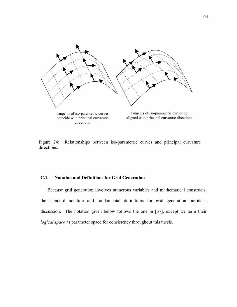
63
C.1. Notation and Definitions for Grid Generation
Because grid generation involves numerous variables and mathematical constructs,
the standard notation and fundamental definitions for grid generation merits a
discussion. The notation given below follows the one in [37], except we term their
logical space as parameter space for consistency throughout this thesis.
Tangents of iso-parametric curves coincide with principal curvature
directions
Tangents of iso-parametric curves not aligned with principal curvature directions
Figure 24: Relationships between iso-parametric curves and principal curvature directions.
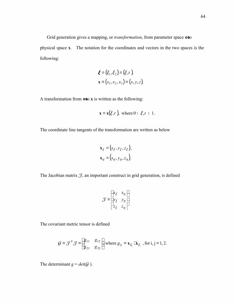
64
Grid generation gives a mapping, or transformation, from parameter space ññññ to
physical space x. The notation for the coordinates and vectors in the two spaces is the
following:
A transformation from ññññ to x is written as the following:
The coordinate line tangents of the transformation are written as below
The Jacobian matrix �, an important construct in grid generation, is defined
The covariant metric tensor is defined
The determinant g = det(� ).
( ) ( )( ) ( ).,,,,
.,,
321
21
zyxxxx ==
==
x
ηξξξξξξξ
( ) .1,0 where,, ≤≤= ηξηξxx
( )( ). ,,
, ,,
ηηηη
ξξξξ
zyx
zyx
=
=
x
x
.
=
η
η
η
ξ
ξ
ξ
zyx
zyx
��
.2 ,1ji,for , where,gg
2221
1211T =⋅=
==
jijggg
ξξ xxi
����

65
C.2. Introduction to Planar Variational Grid Generation
A variational grid generator iteratively minimizes a functional to establish the grid
transformation. A functional I[x] is defined as a function having a set of vectors of
functions for its domain and real numbers for its range [63]. Functionals are formalized
to preserve prescribed geometric properties of the grid. Three common functionals are
the length functional, the area functional, and the orthogonality functional [37]. A
functional has the general form
The length functional optimizes the length of grid line segments and has the form
where Ñ(ññññ) and ó(ññññ) are the coordinate line weight functions. The area functional
optimizes the area of the grid cells and has the form
where Ñ(ññññ) is the area weight function. The orthogonality functional optimizes the
orthogonality of angles between ñ and Ü coordinate lines and has the form
[ ] ( ) . ,,, 1
0
1
0
ξξξξ ηηξ ξddGI ∫ ∫= xxxx
[ ] , gg
21 1
0
1
0
2211 ηψφ
ξddI L ∫ ∫
+=x
[ ] , g 21 1
0
1
0
ηφξddI A ∫ ∫=x
[ ] . g 21 1
0
1
0
212 ηξddIO ∫ ∫=x
66
Oftentimes, the desired grid may exhibit a compromise between these geometric
constraints, requiring the weighted combination functional
For our finite element method, we utilize a fourth functional called the alignment
functional, which seeks to align the grid coordinate lines along two alignment vector
fields v1(x) and v2(x). In essence, the objective is to generate a grid where v1(x) öö xñ and
v2(x) öö xÜ . Biorthogonality establishes that the covariant tangent vectors xñ and xÜ are
orthogonal, respectively, to the contravariant normal vectors Ô x Ü and Ô x ñ, providing the
following conditions:
v1(x) öö xñ ˘ v1(x) ı Ô x Ü = 0
v2(x) öö xÜ ˘ v2(x) ı Ô x ñ = 0.
When the dot product of the contravariant normal vector and the alignment vector equals
zero, the covariant tangent vector is aligned with the alignment vector. Thus, the
functional has the form
As described in the next section, prescribing the principal curvature directional vector
fields to v1(x) and v2(x) aligns the grid coordinate lines to the gyral ribs.
[ ] . OOAALLw IwIwIwI ++=x
[ ] ( ) ( ) . 21 1
0
21
1
0
22 ηηξ ξddI N ∫ ∫ ∇⋅+∇⋅= xx vvx
67
C.3. Variational Grid Generation for Reparameterization
The parameter space ññññ = (ñ, Ü ), 0 ¡ ñ, Ü ¡ 1 for a tensor patch in physical space
x = (x, y, z) often generates undesirable iso-parametric curves on the gyral surface in the
physical domain; this problem can be seen as a skewed density distribution of parameter
space. For example, mapping a uniformly sampled structured grid in ññññ to x can yield a
very disproportionate mesh. The parameter space must be redistributed, or
reparameterized, with a new parameter space r = (r, s) to attain uniformly spaced meshes
in x for uniformly spaced meshes in r. Desirable characteristics for the mapping from
parameter space to physical space extend beyond uniform length or area. For
neocortical decomposition, gyral rib boundary constraints require that the tangents of
iso-parametric curves coincide with principal curvature directions.
Determining the reparameterization, or transformation, from r to x is, indeed, a
planar grid generation problem. The mapping from the new parameter space r to
physical space x is now defined by two transformations: one from r to ññññ via the grid
mapping and the second from ññññ to x via the tensor patch parameterization, which
remains unchanged throughout the process. A regular grid in r now corresponds to finite
element boundaries on the gyral surface in physical space (see Figure 25).
This application of variational grid generation requires two formulations: (1) a
reference template and (2) a functional guiding the variational grid generation. First, the
macro element is trimmed from the gyral surface with a four-sided template, called a
reference template, to produce a trimmed surface. A reference template is a
quadrilateral that provides the boundary conditions necessary for grid generation. A
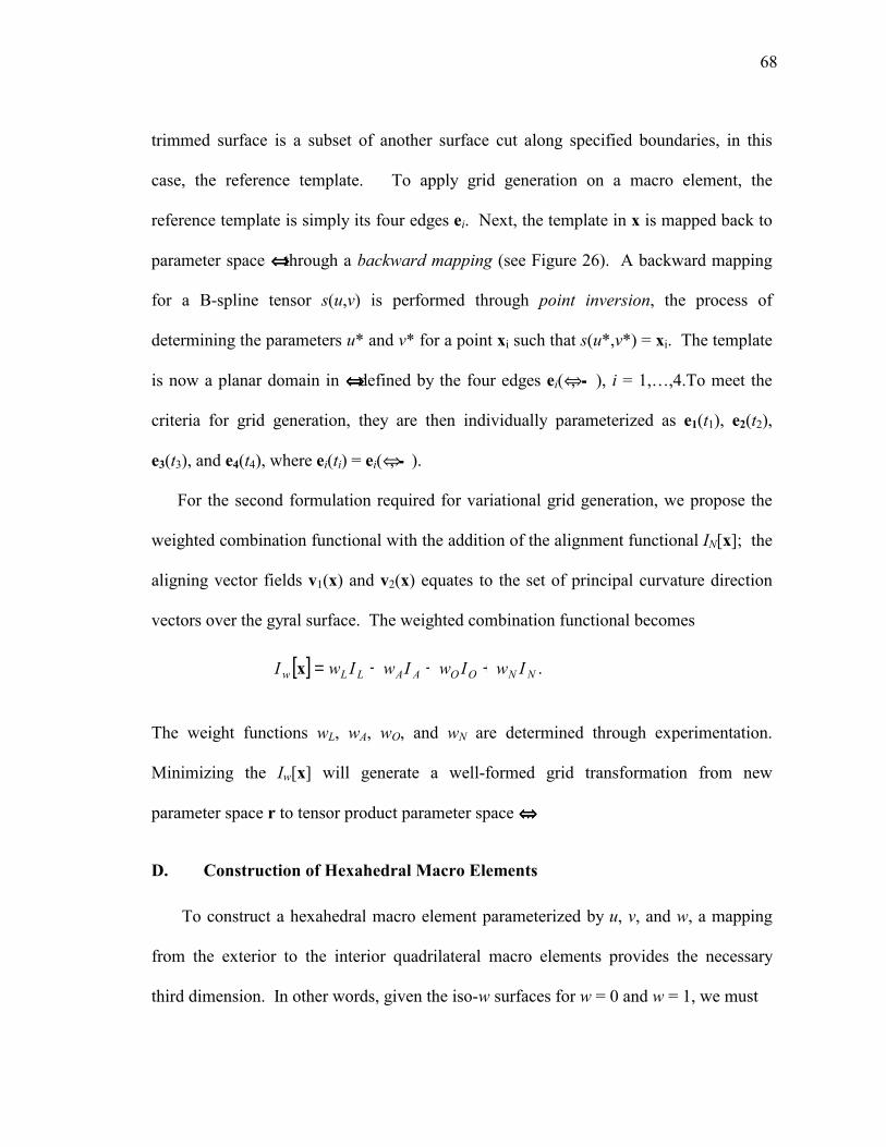
68
trimmed surface is a subset of another surface cut along specified boundaries, in this
case, the reference template. To apply grid generation on a macro element, the
reference template is simply its four edges ei. Next, the template in x is mapped back to
parameter space ññññ through a backward mapping (see Figure 26). A backward mapping
for a B-spline tensor s(u,v) is performed through point inversion, the process of
determining the parameters u* and v* for a point xi such that s(u*,v*) = xi. The template
is now a planar domain in ññññ defined by the four edges ei(ñ, Ü ), i = 1,�,4.To meet the
criteria for grid generation, they are then individually parameterized as e1(t1), e2(t2),
e3(t3), and e4(t4), where ei(ti) = ei(ñ, Ü ).
For the second formulation required for variational grid generation, we propose the
weighted combination functional with the addition of the alignment functional IN[x]; the
aligning vector fields v1(x) and v2(x) equates to the set of principal curvature direction
vectors over the gyral surface. The weighted combination functional becomes
The weight functions wL, wA, wO, and wN are determined through experimentation.
Minimizing the Iw[x] will generate a well-formed grid transformation from new
parameter space r to tensor product parameter space ññññ.
D. Construction of Hexahedral Macro Elements
To construct a hexahedral macro element parameterized by u, v, and w, a mapping
from the exterior to the interior quadrilateral macro elements provides the necessary
third dimension. In other words, given the iso-w surfaces for w = 0 and w = 1, we must
[ ] .NNOOAALLw IwIwIwIwI +++=x
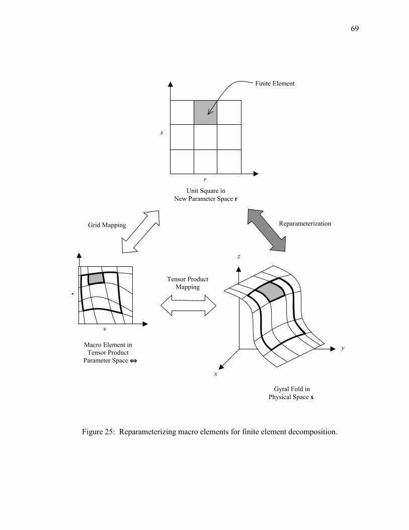
69
x
y
z
Grid Mapping
Tensor Product Mapping
r
s
Unit Square in New Parameter Space r
Macro Element in Tensor Product
Parameter Space ññññ
Gyral Fold in Physical Space x
Figure 25: Reparameterizing macro elements for finite element decomposition.
Reparameterization
ñ
Ü
Finite Element
70
now "fill in" the dimension parameterized by 0 < w < 1. For neuroanatomical
consistency, the iso-uv curves within the hexahedral macro element should coincide with
the mean axes of growth for pyramidal cells inside the tissue segment. Conceptually, a
smooth morph from the interior surface to the exterior surface should trace out the mean
axes of growth.
Absent the structural data for pyramidal cells, we model the axes with line segments
constructed by linearly interpolating between points on the exterior and interior surfaces
that correspond in parameter space. For example, the line segment connecting the points
sexterior(0.5,0.5) and sinteior(0.5,0.5) would be a pyramidal cell growth axis. As shown in
[4], this linear interpolation is valid for axes stemming from ridge or valley lines on the
neocortical tissue. The development of a consistent model for the mean axes of growth
requires further research and empirical or statistical data.
ñ
Ü
x
y
z
Reference Template
Backward Mapping
Forward Mapping
Figure 26: Propagation of reference template to tensor product parameterspace.

71
E. Division into Hexahedral Finite Elements
The finite element is the volume bounded by six coordinate surfaces (two coordinate
surfaces for each parameter u, v, and w) in the hexahedral finite element. Iso-w planes
are simply the exterior and interior neocortical surfaces at w = 0 and w = 1. Varying the
u and v coordinates, in effect, controls the shape and size of the generated finite
elements. For neuroanatomical consistency, the bounding u coordinates are the ith and
(i + 2)th knots from the u knot vector of the tensor B-spline patch; likewise, the
bounding v coordinates are determined in the same manner for the v knot vector. Our
empirical results suggest cutting the macro element at every second knot in both u and v
directions; this slicing produced finite elements with edges no more geometrically
complex then cubic Bezier curves. The decomposed finite elements are, thus,
guaranteed to be geometrically simple and relatively uniform in size.
72
CHAPTER VII
OBJECT-ORIENTED SOFTWARE TOOLS
A. Introduction
We developed a suite of object-oriented software tools for the finite element
decomposition of the human neocortex and the visualization of the results at each stage.
The object classes developed in ANSI C++ are fully compatible with the Visualization
Toolkit v1.3 (vtk), FITPACK, and NUAGES. Further, the objects share file format with
Elastic Reality (Avid Technology, Inc.).
B. Brief Descriptions of Software Tools
From our object classes, we developed six software tools. They all furnish a mouse-
driven interactive visualization environment and are briefly described below:
• B-spline Contourer. The utility fits univariate smoothing B-splines to cross
sections of polygonal contours. Supporting features include intersection
detection and correction, sectional viewing, reparametrization, and consolidation
of contour segments into a single contour curve.
• Contour Correspondence Tool. The tool provides an interactive environment for
the correspondence of contours into anatomical objects and facilitates the
conversion of the contours to a dataset ready for surface fitting. It outputs data
files ready for either Delaunay-based surface reconstruction or tensor surface
73
fitting. Supporting features include landmarking, reparameterization, and
viewing in parameter space.
• Mesh Viewer. This utility provides an interactive environment for viewing
reconstructed surface meshes and the computation of principal curvatures and
directions. Supporting features include the color mapping of shape metrics onto
the mesh, interactive region extraction, and sectional viewing.
• Segment Extractor. This tool provides an interactive environment for the rapid
extraction of neocortical tissue segments by tracing them through the coronal
cutting plane. It outputs the tissue segments either as polygons or B-splines.
• Tensor Surface Fitter. This utility fits smoothing tensor B-splines to a set of
consecutive planar contours and provides various plots for curvature information
of the surface. The user can interactively alter the sampling, parameterization,
and smoothness of the fit.
• Finite Element Decomposer. This tool decomposes a tensor surface model into
finite elements ready for grid generation.
The suite of tools utilize two software libraries and work with two third-party
applications to complete the process from contour extraction to finite element
decomposition. The four supporting software programs are described below.
• Visualization Toolkit. The vtk class library includes a comprehensive object
model of geometric primitives and algorithms for both numerical computation
and visualization [56]. The library extends to higher-level data structures and
algorithms, e.g. tensors, hyperstreamlines, glyphs, marching cubes, and mesh
74
decimation. In addition, vtk is compatible with numerous graphical formats.
Our object classes are integrated with the vtk classes through containment and
function compatibility. The library is freely available (http://nswt.tuwien.ac.at/
htdocs/vtk/vtkData/HowToGetSoftware.html).
• FITPACK. The FORTRAN library provides functions for data fitting with
smoothing B-splines in various domains and utilities for evaluating partial
derivatives and integrals [16]. Part of the library is available as public domain
software (http://netlib2.cs.utk.edu/fitpack/).
• NUAGES. The command-line driven program takes as input a set of planar
sections consisting of non-intersecting closed polygons and reconstructs a
tetrahedral solid or triangulated surface based on the Delaunay triangulation [25].
The program outputs to numerous file formats, such as OBJ, IDX, and VRML
1.0. The program is available as public domain software (http://www.inria.fr/
prisme/personnel/geiger/nuages.html).
• Elastic Reality. The commercial software for 2D morphing offers a GUI
interface for outlining curves on a set of 2D images. The curves are represented
in cubic Bezier splines and output as a convenient text file. We primarily used
the program for manual contour extraction.
C. Application of Software Tools to the Human Neocortex
Our methodology for the finite element decomposition of the human necortex
produces a finite element model from a set of planar contours in five stages: (1) contour
75
extraction, (2) polygonal surface reconstruction, (3) decomposition into major gyri, (4)
tensor patch fitting, and (5) finite element decomposition. Below is an outline of how
the software tools and the four third-party applications are applied at each stage.
In the first stage, contours for the exterior and interior surface of the human necortex
are manually traced using Elastic Reality. For the work reported here only the right
hemisphere of one human brain was traced. The tracing supplied 271 planar contours,
represented as segments of cubic Bezier splines, cut through the coronal plane. B-spline
Contourer consolidates the fragments of cubic Bezier splines belonging to the same
closed contour and converts them into smoothing B-splines.
In the second stage, Contour Correspondence Tool was used to interactively
correspond contours belonging to the same anatomical parts. The correspondence step is
optional since Delaunay-based surface reconstruction provides its own solution to the
correspondence problem. Alternatively, Contour Correspondence Tool is useful for
selecting a subset of planar sections for reconstruction, i.e. contours can be from the
entire hemisphere or restricted to segments of neocortical tissue. NUAGES rapidly
reconstructs triangulated surfaces for the dataset of contours.
In the third stage, Segment Extractor provides an interactive environment to rapidly
extract the major gyri for a coarse anatomical decomposition of the neocortex. It
represents contours as either B-splines for tensor patch fitting or as closed polygons for
Delaunay-based surface reconstruction.
In the fourth stage, Tensor Surface Fitter fits B-spline tensor patches to the major
gyri. The user can interactively define the patches and vary the sampling rate and

76
smoothness to achieve a desirable fitting. The program outputs a cover of the surface
defined by the input data as a network of patches.
In the fifth stage, Finite Element Decomposer takes as input surface patches for both
the exterior and interior surface of the neocortex and decomposes the B-rep model into
hexahedral finite elements ready for grid generation.

77
CHAPTER VIII
RESULTS
A. Contour Extraction
The dataset for solid model reconstruction consists of 271 x 512 x 512 images of a
76-year-old normal female human cadaver brain cryosectioned through the coronal plane
[61]. Contours of the exterior and interior surfaces of the neocortex are manually traced
using Elastic Reality, a third party application from Avid Technologies, Inc. (see
Figure 27). Tissue segmentation is performed manually with the guided expertise of a
neuroanatomist. Because of the precision and consistency of the cryosectioning
technique, vertical spatial alignment of the consecutive images along the cutting axis
automatically insures the registration of the contours between adjacent sections. The
contours are represented as smooth B-splines. For the work reported here only the right
hemisphere of one human brain was extracted. Figure 28 shows a set of ten consecutive
contours for the exterior neocortical surface extracted using this technique.
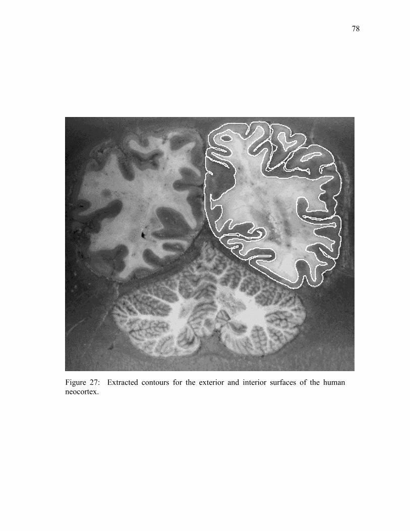
78
Figure 27: Extracted contours for the exterior and interior surfaces of the humanneocortex.
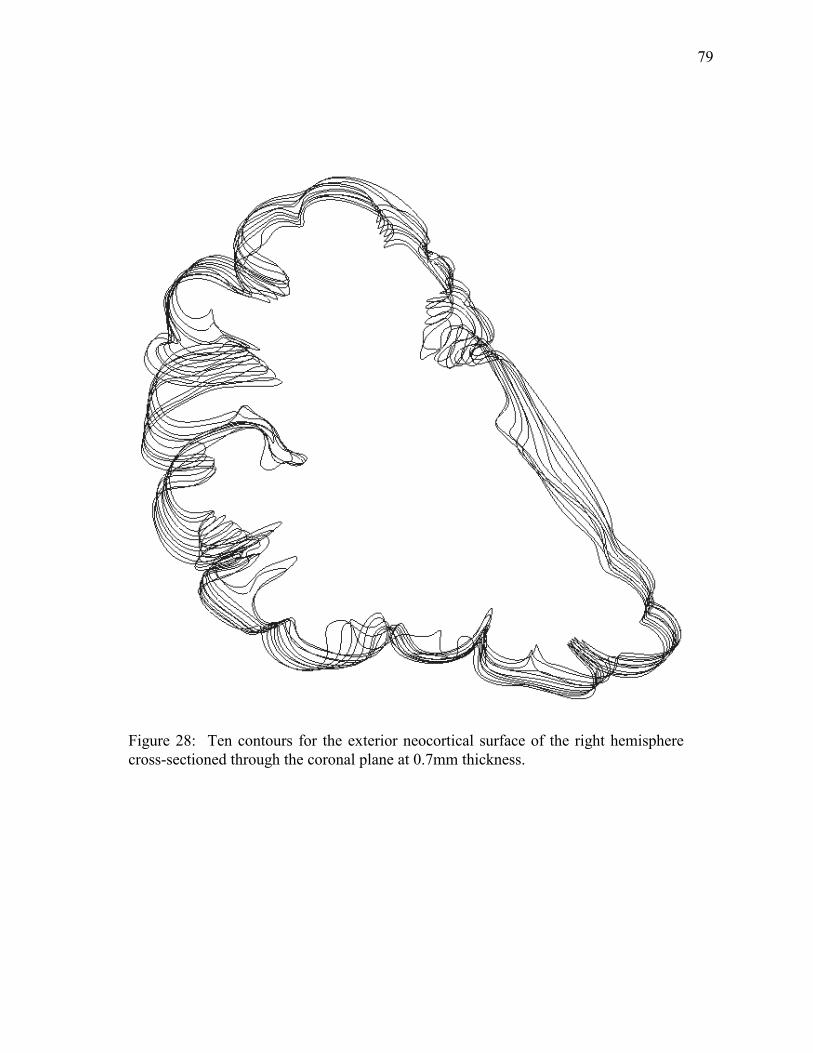
79
Figure 28: Ten contours for the exterior neocortical surface of the right hemispherecross-sectioned through the coronal plane at 0.7mm thickness.

80
B. Solid Model Reconstruction of the Right Hemisphere
Surface reconstruction over the contour dataset produced a cortical shell defined by
the exterior and interior surfaces of the neocortex. The boundary representation (B-rep)
model was constructed using NUAGES, a software utility for Delaunay-based surface
reconstruction [25]. The B-spline contours were sampled using uniform arc-length
parameterization to yield the set of closed polygons required by NUAGES. Volume was
minimized to give the "tightest" triangulation.
Two triangulated meshes, representing the exterior and interior surfaces, defined the
enclosed volume of the neocortex. The outer surface consisted of 69K vertices and
136K triangles; the inner surface consisted of 35K vertices and 77K triangles. Figure 29
and Figure 30 show the reconstructed exterior and interior surfaces with shape index
color mapping to accentuate the convolutions.
The software utility NUAGES also provided as output a tetrahedral representation of
the neocortex. Figure 31 shows an angular view of the tetrahedral reconstruction.
Figure 32 shows cross-sectional view of the reconstructed neocortex. Figure 33
replicates the convenient views offered in Duvernoy's The Human Brain: Surface,
Three-Dimensional Sectional Anatomy and MRI.
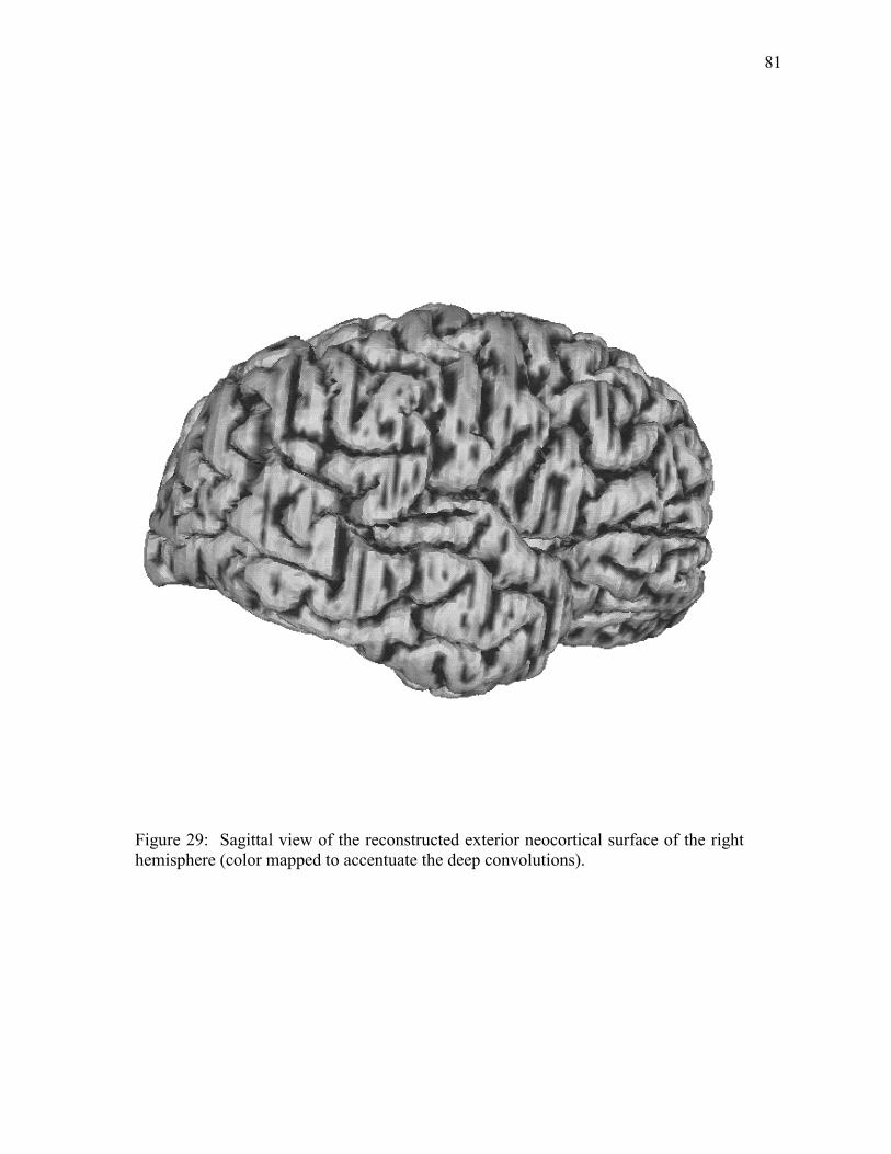
81
Figure 29: Sagittal view of the reconstructed exterior neocortical surface of the righthemisphere (color mapped to accentuate the deep convolutions).
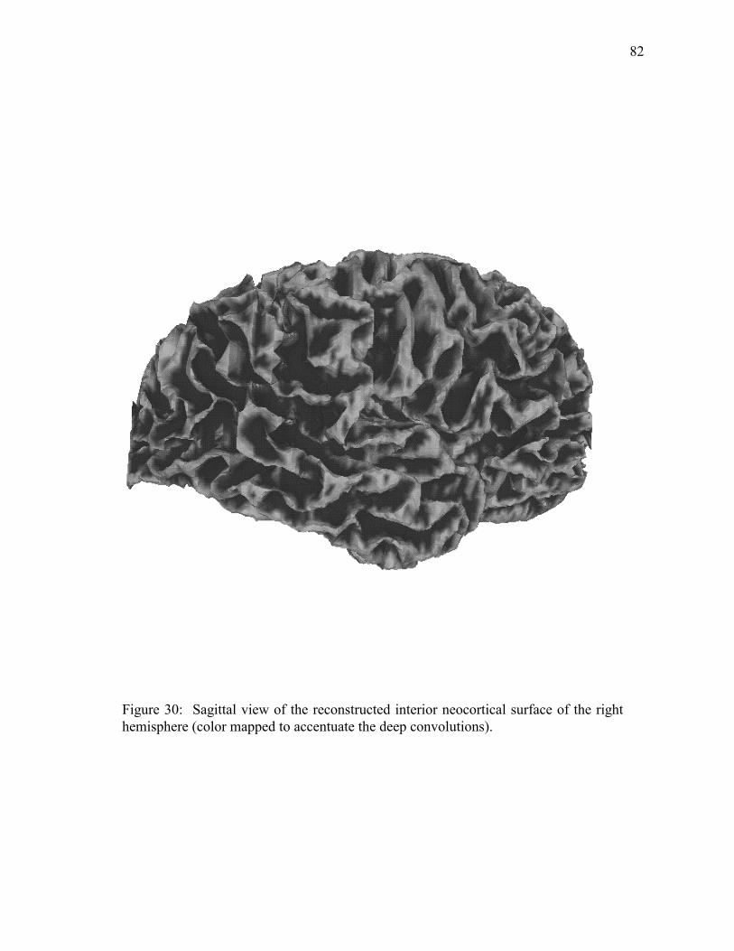
82
Figure 30: Sagittal view of the reconstructed interior neocortical surface of the righthemisphere (color mapped to accentuate the deep convolutions).
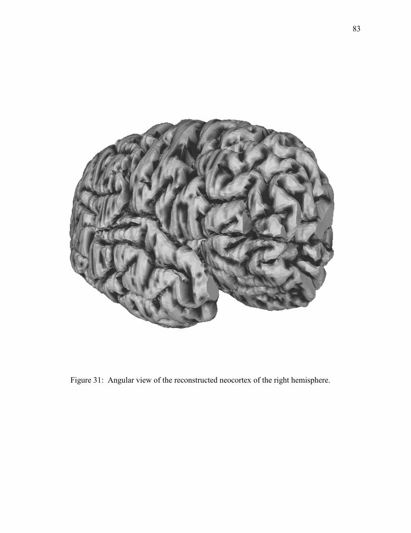
83
Figure 31: Angular view of the reconstructed neocortex of the right hemisphere.
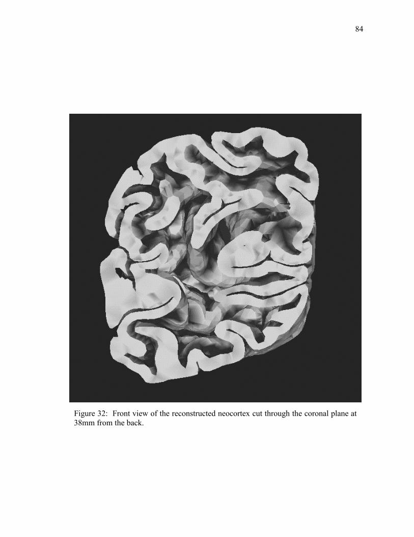
84
Figure 32: Front view of the reconstructed neocortex cut through the coronal plane at38mm from the back.
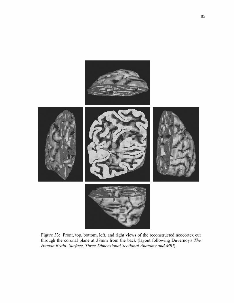
85
Figure 33: Front, top, bottom, left, and right views of the reconstructed neocortex cutthrough the coronal plane at 38mm from the back (layout following Duvernoy's TheHuman Brain: Surface, Three-Dimensional Sectional Anatomy and MRI).
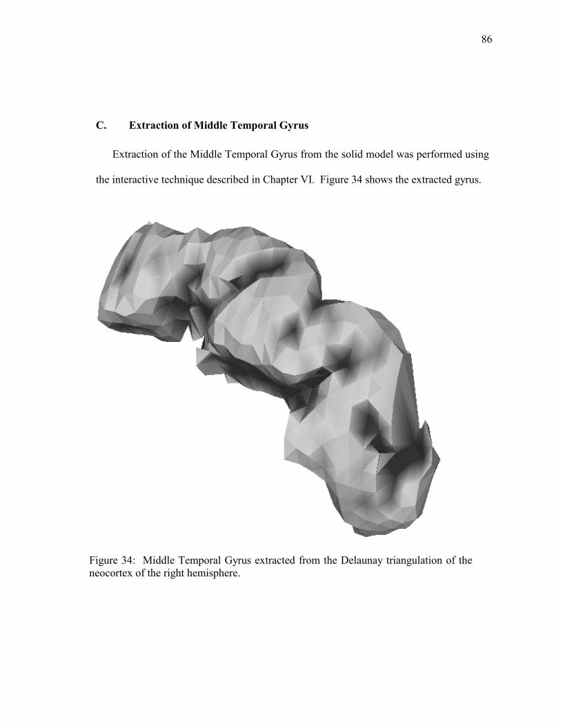
86
C. Extraction of Middle Temporal Gyrus
Extraction of the Middle Temporal Gyrus from the solid model was performed using
the interactive technique described in Chapter VI. Figure 34 shows the extracted gyrus.
Figure 34: Middle Temporal Gyrus extracted from the Delaunay triangulation of theneocortex of the right hemisphere.
87
D. Macro Element Decomposition
Macro element decomposition for the mapped template approach was performed for
the Middle Temporal Gyrus using the techniques described in Chapter VI. The
procedure resulted in six quadrilateral macro elements for the exterior surface and six
corresponding quadrilateral macro elements for the interior surface. By exploiting the
contour containment property of Delaunay-based reconstruciton, contours were retrieved
from the original dataset for B-spline surface fitting to avoid loss in detail. The exterior
and interior gyral surfaces were decomposed separately. Figure 35 and Figure 36 outline
the identification procedure for the gyral line of symmetry; Figure 37 and Figure 38
show the six quadrilateral macro elements resulting from the decomposition. The
quadrilateral macro elements are represented as B-spline tensor patches.
E. Feature Extraction for Reparameterization
Feature information was extracted for the reparameterization technique described in
Chapter VI. Neither grid generation nor reparameterization was conducted for the work
reported in this thesis; however, the developed software tools provide the necessary
datasets needed for the reparameterization. Figure 39 and Figure 40 show the feature
information for a sample gyral surface.
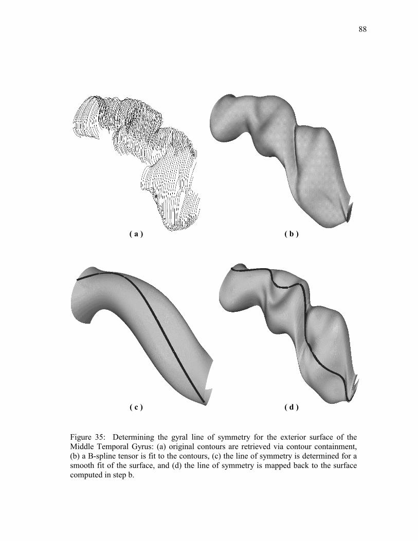
88
( a )
( d )
( b )
( c )
Figure 35: Determining the gyral line of symmetry for the exterior surface of theMiddle Temporal Gyrus: (a) original contours are retrieved via contour containment,(b) a B-spline tensor is fit to the contours, (c) the line of symmetry is determined for asmooth fit of the surface, and (d) the line of symmetry is mapped back to the surfacecomputed in step b.
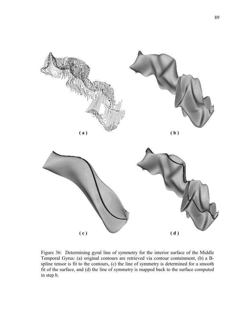
89
( a )
( d )
( b )
( c )
Figure 36: Determining gyral line of symmetry for the interior surface of the MiddleTemporal Gyrus: (a) original contours are retrieved via contour containment, (b) a B-spline tensor is fit to the contours, (c) the line of symmetry is determined for a smooth fit of the surface, and (d) the line of symmetry is mapped back to the surface computedin step b.
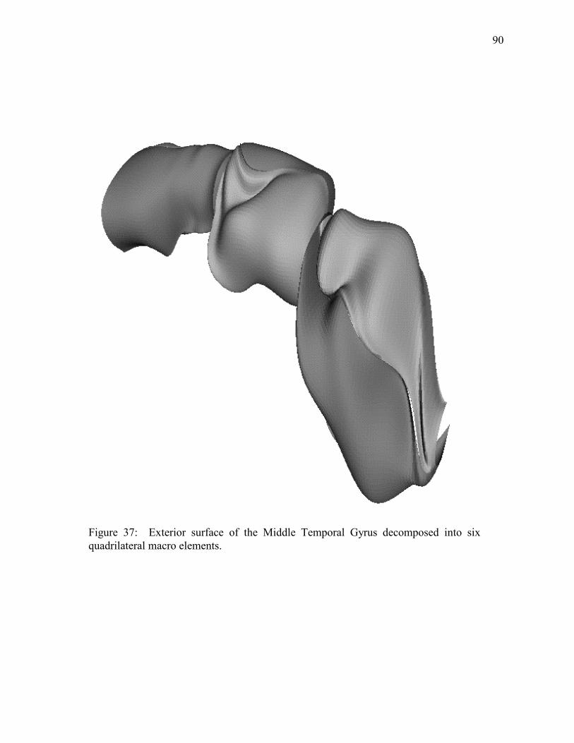
90
Figure 37: Exterior surface of the Middle Temporal Gyrus decomposed into sixquadrilateral macro elements.
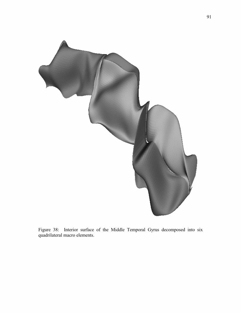
91
Figure 38: Interior surface of the Middle Temporal Gyrus decomposed into sixquadrilateral macro elements.
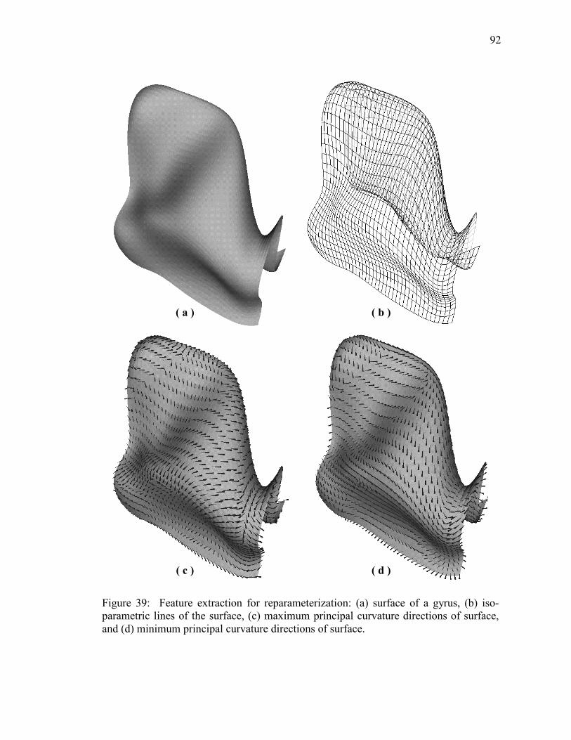
92
( a )
( d )
( b )
( c )
Figure 39: Feature extraction for reparameterization: (a) surface of a gyrus, (b) iso-parametric lines of the surface, (c) maximum principal curvature directions of surface,and (d) minimum principal curvature directions of surface.
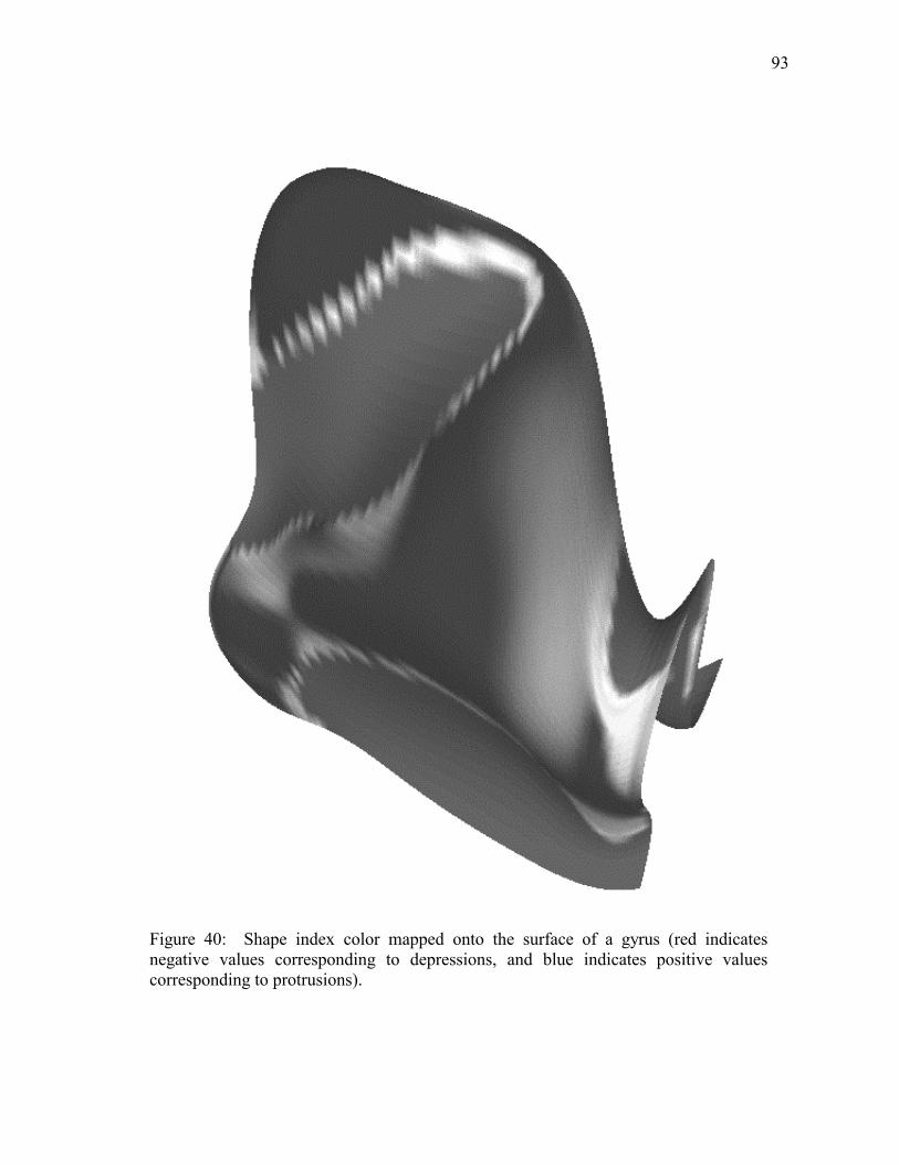
93
Figure 40: Shape index color mapped onto the surface of a gyrus (red indicatesnegative values corresponding to depressions, and blue indicates positive valuescorresponding to protrusions).

94
F. Finite Element Decomposition
The Middle Temporal Gyrus was decomposed into hexahedral finite elements using
the mapped template approach and the techniques described in Chapter VI. Two
corresponding quadrilateral macro elements from the exterior and interior surfaces
define the top and bottom sides of a hexahedral macro element. Lacking the data for
mean axes of growth of pyramidal cells within the tissue segment, the other four sides
are constructed using simple linear interpolation from the exterior macro element to the
interior macro element. As described in [4], this linear interpolation closely
approximates the pyramidal cell growth axes at ridge and valley lines of the macro
element. Figure 41 outlines the decomposition of a macro element into finite elements.
Figure 42 and Figure 43 show two views of the hexahedral finite elements for a tissue
segment from the Middle Temporal Gyrus. The segment actually consists of two
hexahedral macro elements. Figure 44, 45, and 46 show different views of the
decomposed hexahedral finite elements for the Middle Temporal Gyrus.
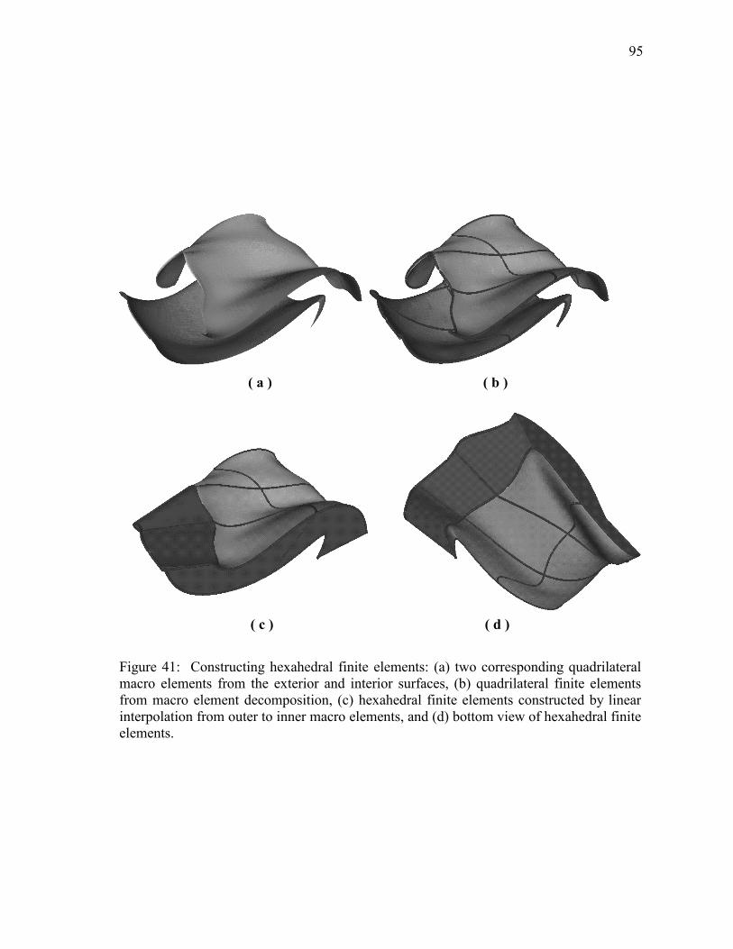
95
( a )
( d )
( b )
( c )
Figure 41: Constructing hexahedral finite elements: (a) two corresponding quadrilateralmacro elements from the exterior and interior surfaces, (b) quadrilateral finite elementsfrom macro element decomposition, (c) hexahedral finite elements constructed by linearinterpolation from outer to inner macro elements, and (d) bottom view of hexahedral finiteelements.
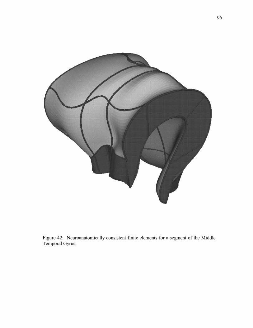
96
Figure 42: Neuroanatomically consistent finite elements for a segment of the MiddleTemporal Gyrus.
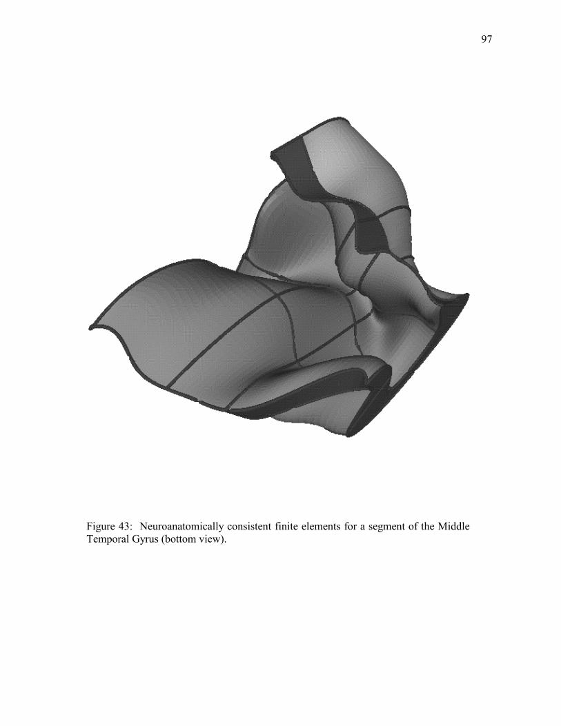
97
Figure 43: Neuroanatomically consistent finite elements for a segment of the MiddleTemporal Gyrus (bottom view).
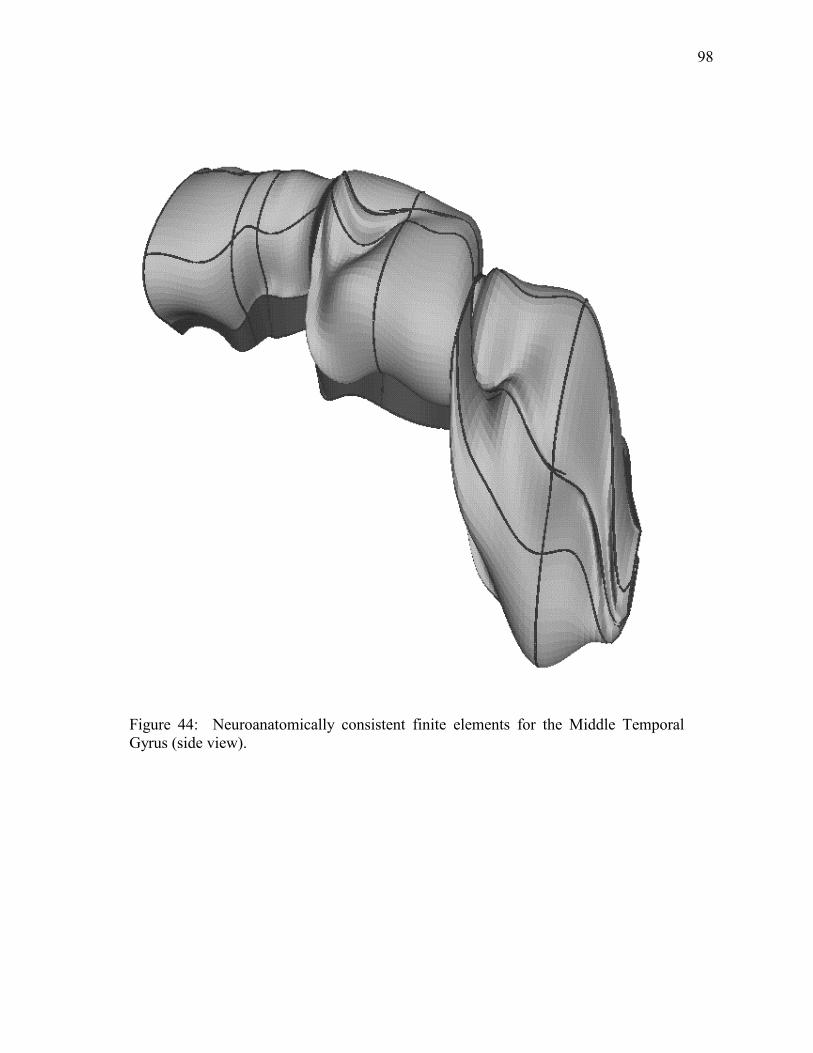
98
Figure 44: Neuroanatomically consistent finite elements for the Middle TemporalGyrus (side view).
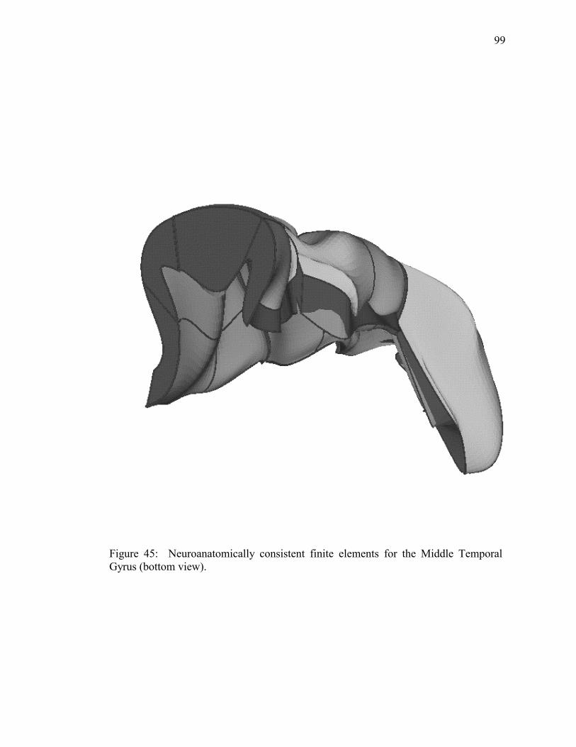
99
Figure 45: Neuroanatomically consistent finite elements for the Middle TemporalGyrus (bottom view).

100
Figure 46: Neuroanatomically consistent finite elements for the Middle TemporalGyrus (front view).
101
CHAPTER VIII
SUMMARY AND FUTURE WORK
A. Summary
A method for the decomposition of the human neocortex into hexahedral finite
elements is presented. The technique adopts the mapped template approach and follows
the constraints defined by neuroanatomical consistency. The finite element model
provides both the necessary boundary conditions for numerical grid generators and a
structural information framework. A new class library and a set of object-oriented
software tools were developed to implement the decomposition method. For the work
reported in this thesis, the neocortex for the right hemisphere of a cadaver human brain
was reconstructed; finite element decomposition was performed for the Middle
Temporal Gyrus; and the feature information necessary for reparameterization were
computed.
B. Future Work
Many steps in our neocortical finite element decomposition method can be expedited
with automated techniques and can be extended when empirical data is available. Below
is a list of future improvements:
1. Automate the contour extraction. Even with the convenient tracing environment
provided in Elastic Reality, manually tracing the contours of the neocortical
102
tissue requires significant user intervention. For the work reported in this thesis,
this step poses the biggest bottleneck of the decomposition process.
2. Automate the extraction of major gyri. The anatomical division of the
neocortex into major gyri is the most important step of the mapped template
approach. Besides enforcing neuroanatomical consistency, the division ensures
the creation of well-formed templates for tensor spline fitting. The software tool
developed for this thesis allows relatively fast and convenient extrication of
major gyri; however, an automated technique would speed up the process and
may lead to a better understanding of the brain's spatial structure. This coarse-
level division remains a general challenge for the mapped template approach.
3. Fully automate the identification of the gyral line of symmetry. Our semi-
automatic multi-resolution method rapidly identifies the line of symmetry, but it
still requires user intervention. An automated technique would further expedite
the decomposition. Without a direct correlation between the geometric features
of the gyral surface and the gyral line of symmetry, automatic detection of this
dividing boundary remains an imposing obstacle.
4. Automate the identification of sectional cutting curves. As described in Chapter
VI, cutting the gyrus at sharp bends of its medial axis help ensure well-formed
macro elements (templates). Automating the identification of sectional curves
requires the automatic construction of the medial axis or medial manifold for a
major gyrus. Such an automated technique should exploit the close relationship
between the medial axis and the Delaunay triangulation.

103
5. Represent the hexahedral finite elements as tricubic meshes. As described in
[4], 3D grid generation provides a local coordinate system within the finite
element if its geometry is relatively simple. Many robust grid generators are
available to construct a grid for a volume bounded by curvilinear edges
representable with cubic Bezier curves. The hexahedral finite elements for the
work reported in this thesis exhibit the required geometric simplicity, but they
need to be fitted with tricubic interpolation to establish the boundary constraints
necessary for grid generation.
6. Reparameterize the macro elements. The reparameterization, described in
Chapter VI, to align coordinate lines of the finite element mesh with the
tangents of the principal curvature directions of the gyral surface was not
implemented for the work reported in this thesis. The macro elements for the
Middle Temporal Gyrus did not require reparameterization for the
decomposition along gyral ribs. However, other major gyri, especially those
located in the parietal lobe, will require reparameterization for neuroanatomical
consistency.
7. Establish a data structure for the spatial management of the finite elements. The
hierarchical subdivision of the neocortex, from anatomical lobes to the finite
elements, presents a natural framework for the spatial organization of the
elements. Before the finite element model can be integrated into a structural
information framework, a data structure needs to be established to facilitate the
indexing and organization of the elements.
104
8. Export the finite element model to an Internet compliant platform. Besides
spatial organization, one of the primary objectives of the structural information
framework is to provide wide accessibility of the model through the Internet.
To achieve wide distribution, one can either develop a client resident applet to
view the B-spline representation of the solid model or export the model to a
graphical format, such as VRML 2.0.
9. Model the mean axes of growth of pyramidal cells inside the finite elements.
When statistical data for the structure of pyramidal cells is available, the axes of
growth can define the mapping from the interior gyral surface to the exterior
gyral surface. The iso-uv curves of the local coordinate system within each
finite element would then coincide with the mean axes of growth of pyramidal
cells inside the tissue segment.
10. Embed graphical models of neurons into the finite elements. When statistical
data for neuron populations within the neocortex is available, stochastically
generated neurons can be embedded inside the finite elements.
11. Model the afferent and efferent fibers of the finite elements. The finite element
decomposition provides the framework for the modeling of the afferent and
efferent fiber network of the neocortex. The development of such a model
requires presently absent empirical data and a connectivity model outside the
scope of this thesis.
105
REFERENCES
[1] L. Alboul and R. Van Damme, "Polyhedral Metrics in Surface Reconstruction," in Mathematics on Surface VI, pp. 171-200, Ed. G. Mullineux. Oxford: Clarendon Press, 1996.
[2] V. Algazi, B. Reutter, W. van Warmerdam, and C. Liu, "Three-Dimensional Image Analysis and Display by Space-Scale Matching of Cross Sections," J. Opt. Soc. Am., Vol. 6, No. 6, 1989.
[3] S. Batnitzky, H. Price, P. Cook, L. Cook, and S. Dwyer III, "Three-Dimensional Computer Reconstruction from Surface Contours for Head CT Examinations," Journal of Computer Assisted Tomography, Vol. 5, No. 1, pp. 60-67, 1981.
[4] D. A. Batte, "Finite Element Decomposition and Grid Generation for Brain Modeling and Visualization." M.S. Thesis, Department of Computer Science, Texas A&M University, 1997.
[5] M. de Berg, M. van Kreveld, M. Overmans, and O. Schwarzkopf, Computational Geometry. Berlin: Springer, 1997.
[6] T. Blacker and R. Meyers, "Seams and Wedges in Plastering: A 3-D Hexahedral Mesh Generation Algorithm," Engineering with Computers, Vol. 9, pp. 83-93, 1993.
[7] T. Blacker and M. Stephenson, "Paving: A New Approach to Automated Quadrilateral Mesh Generation," International Journal for Numerical Methods in Engineering, Vol. 32, pp. 811-847, 1991.
[8] R. Bolle and B. Vemuri, "On Three-Dimensional Surface Reconstruction Methods," IEEE Transactions of Pattern Analysis and Machine Intelligence, Vol. 13, No. 1, 1991.
[9] J. Boissonnat, "Shape Reconstruction from Planar Cross Sections," Computer Vision, Graphics, and Image Processing, Vol. 44, pp. 1-29, 1988.
[10] J. Boissonnat and B. Geiger, "Three Dimensional Reconstruction of Complex Shapes Based on the Delaunay Triangulation," INRIA Rapports de Recherche, No. 1697, 1992. Availabe at http://www.inria.fr/RRRT/publications-eng.html.
[11] Brinkley, J. F., "Structural Informatics and Its Applications in Medicine and Biology," Academic Medicine, Vol. 66, pp. 589-591, 1991.
[12] B. Burton, T. Chow, A. Duchowski, and B. McCormick, "Exploring the Brain Forest," Computational Neuroscience '98 (CNS*98) Submission, January 1998.
[13] G. Carman, H. Drury, D. Van Essen, "Computational Methods for Reconstructing and Unfolding the Cerebral Cortex, Cerebral Cortex, Vol. 5, pp. 506-517, 1995.
106
[14] M. do Carmo, Differential Geometry of Curves and Surfaces. Englewood Cliffs, New Jersey: Prentice-Hall, Inc., 1976.
[15] R. Cass, S. Benzley, R. Meyers, and T. Blacker, "Generalized 3-D Paving: An Automated Quadrilateral Surface Mesh Generation Algorithm," International Journal for Numerical Methods in Engineering, Vol. 39, pp. 1475-1489, 1996.
[16] P. Dierckx. Curve and Surface Fitting with Splines. Oxford: Clarendon Press, 1995.
[17] H. Drury and D. Van Essen, "Functional Specializations in Human Cerebral Cortex Analyzed Using the Visible Man Surface-Based Atlas," Human Brain Mapping, Vol. 5, No. 4, pp. 233-237, 1997.
[18] H. Drury, D. Van Essen, C. Anderson, C. Lee, T. Coogan, and J. Lewis, "Computerized Mappings of the Cerebral Cortex: A Multiresolution Flattening Method and a Surface-Based Coordinate System," Journal of Cognitive Neuroscience, Vol. 8, No. 1, pp. 1-28, 1996.
[19] H. Duevnoy. The Human Brain: Surface, Three-Dimensional Sectional Anatomy and MRI. New York: Springer-Verlag Wien, 1991.
[20] M. Eck and H. Hoppe, "Automatic Reconstruction of B-spline Surfaces of Arbitrary Topological Type," Computer Graphics (SIGGRAPH '96 Proceedings), pp. 102, August 1996.
[21] G. Elber and E. Cohen, "Second-Order Surface Analysis Using Hybrid Symbolic and Numeric Operators," ACM Transcations on Graphics, Vol. 12, No. 2, pp. 160-178, 1993.
[22] G. Farin, Curves and Surfaces for CAGD, 3rd Ed. San Diego: Academic Press, Inc., 1993.
[23] G. Farin and H. Hagen, "A Local Twist Estimator," in Topics in Surfae Modeling, H. Hagen, eds., pp. 79-84. Philadelphia: SIAM, 1992.
[24] D. Flip, "Blending Parametric Surfaces," ACM Transactions on Graphics, Vol. 8, No. 3, pp. 164-173, 1989.
[25] B. Geiger, "Three Dimensional Modeling of Human Organs and its Application to Diagnosis and Surgical Planning," INRIA Rapports de Recherche, No. 2105, 1993. Available at http://www.inria.fr/RRRT/publications-eng.html.
[26] S. Guan, "Guided Image Interpretation in Neuroanatomy," Ph.D. Dissertation, Department of Computer Science, Texas A&M University, 1991.
[27] A. Guezeic and D. Dean, "The Wrapper: A Surface Optimization Algorithm That Preserves Highly Curved Areas," SPIE, Vol. 2359, 1994.
[28] A. Gueziec and R. Hummel, "Exploiting Triangulated Surface Extraction Using Tetrahedral Decomposition," IEEE Transactions on Visualization and Computer Graphics, Vol. 1, No. 4, pp. 328-342, 1995.
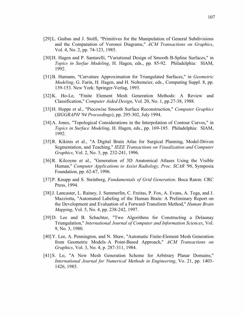
107
[29] L. Guibas and J. Stolfi, "Primitives for the Manipulation of General Subdivisions and the Computation of Voronoi Diagrams," ACM Transactions on Graphics, Vol. 4, No. 2, pp. 74-123, 1985.
[30] H. Hagen and P. Santarelli, "Variational Design of Smooth B-Spline Surfaces," in Topics in Surfae Modeling, H. Hagen, eds., pp. 85-92. Philadelphia: SIAM, 1992.
[31] B. Hamann, "Curvature Approximation for Triangulated Surfaces," in Geometric Modeling, G. Farin, H. Hagen, and H. Noltemeier, eds., Computing Suppl. 8, pp. 139-153. New York: Springer-Verlag, 1993.
[32] K. Ho-Le, "Finite Element Mesh Generation Methods: A Review and Classification," Computer Aided Design, Vol. 20, No. 1, pp.27-38, 1988.
[33] H. Hoppe et al., "Piecewise Smooth Surface Reconstruction," Computer Graphics (SIGGRAPH '94 Proceedings), pp. 295-302, July 1994.
[34] A. Jones, "Topological Considerations in the Interpolation of Contour Curves," in Topics in Surface Modeling, H. Hagen, eds., pp. 169-185. Philadelphia: SIAM, 1992.
[35] R. Kikinis et al., "A Digital Brain Atlas for Surgical Planning, Model-Driven Segmentation, and Teaching," IEEE Transactions on Visualization and Computer Graphics, Vol. 2, No. 3, pp. 232-241, 1996.
[36] R. Kilcoyne et al., "Generation of 3D Anatomical Atlases Using the Visible Human," Computer Applications to Assist Radiology, Proc. SCAR '96, Symposia Foundation, pp. 62-67, 1996.
[37] P. Knupp and S. Steinberg, Fundamentals of Grid Generation. Boca Raton: CRC Press, 1994.
[38] J. Lancaster, L. Rainey, J. Summerlin, C. Freitas, P. Fox, A. Evans, A. Toga, and J. Mazziotta, "Automated Labeling of the Human Brain: A Preliminary Report on the Development and Evaluation of a Forward-Transform Method," Human Brain Mapping, Vol. 5, No. 4, pp. 238-242, 1997.
[39] D. Lee and B. Schachter, "Two Algorithms for Constructing a Delaunay Triangulation," International Journal of Computer and Information Sciences, Vol. 9, No. 3, 1980.
[40] Y. Lee, A. Pennington, and N. Shaw, "Automatic Finite-Element Mesh Generation from Geometric Models�A Point-Based Approach," ACM Transactions on Graphics, Vol. 3, No. 4, p. 287-311, 1984.
[41] S. Lo, "A New Mesh Generation Scheme for Arbitrary Planar Domains," International Journal for Numerical Methods in Engineering, Vo. 21, pp. 1403-1426, 1985.
108
[42] R. Löhner, "Progress in Grid Generation via the Advancing Front Technique," Engineering with Computers, Vol. 21, pp. 186-210, 1996.
[43] W. Lorensen and H. Cline, "Marching Cubes: A High Resolution 3D Surface Construction Algorithm," ACM SIGGRAPH, Vol. 21, No. 4, pp. 163-169, Anaheim, California, 1987.
[44] J. Maillot, H. Yahia, and A. Verroust, "Interactive Texture Mapping," Computer Graphics (SIGGRAPH '93 Proceedings), pp. 1-8, August, 1993.
[45] D. Meyers, S. Skinner, and K. Sloan. "Surfaces from Contours," ACM Transactions on Graphics, Vol. 11, No. 3, pp. 228-258, 1992.
[46] A. Middleditch and C. Reade, "A Kernel for Geometric Features," Proceedings of 4th Symposium on Solid Modeling and Applications, Atlanta, Georgia, pp. 131-140, 1997.
[47] E. Milios, "Shape Matching Using Curvature Processes," Computer Vision, Graphics, and Image Processing, Vol. 47, pp. 203-226, 1989.
[48] O. Monga, N. Ayache, and P. Sander, "From voxel to curvature," IEEE Conference on Vision and Pattern Recognition, Hawaii, June 1991.
[49] H. Nowacki and D. Reese, "Design and Fairing of Ship Surfaces," in Surfaces in CAGD, R. E. Barnhill and W. Böhm, eds., North-Holland, Amsterdam, pp. 121-134, 1983.
[50] B. Payne and A. Toga, "Surface Reconstruction by Multiaxial Triangulation," IEEE Computer Graphics and Applications, pp. 28-35, November 1994.
[51] W. Press, S. Teukolsky, W. Vetterling, and B. Flannery. Numerical Recipes in C, 2nd Edition. Cambridge: Cambridge University Press, 1992.
[52] K. Schaper, K. Rehm , D. Sumners, V. Wedeen, S. Strother, J. Anderson, D. Rottenberg, "Symbolic Representation of Functional Data: The Corner-cube Environment," Neuroimage 3 (Suppl.): S166, 1996.
[53] E. Schwartz, B. Merker, E. Wolfson, and A. Shaw, "Applications of Computer Graphics and Image Processing to 2D and 3D Modeling of the Functional Architecture of Visual Cortex," IEEE Computer Graphics and Applications, pp. 13-23, July 1988.
[54] D. Sheehy, C. Armstrong, and D. Robinson, "Shape Description by Medial Surface Construction," IEEE Transactions on Visualization & Computer Graphics, Vol. 2, No. 1, pp. 62-72, 1996.
[55] M. Shepard, "Update to: Approaches to the Automatic Generation and Control of Finite Element Meshes," Applied Mechanics Review, Vol. 49, no. 10, part 2, pp. 5-14, 1996.
[56] W. Shroeder, H. Martin, and B. Lorensen. The Visualization Toolkit. New Jersey: Prentice Hall PTR, 1996.
109
[57] R. Sonthi, G. Kunjur, and R. Gadh, "Shape Feature Determination using the Durvature Region Representation," Proceedings of 4th Symposium on Solid Modeling and Applications, Atlanta, Georgia, pp. 285-295, 1997.
[58] J. Talairach and P. Tournoux, Co-Planar Stereotaxic Atlas of the Human Brain. New York: Thieme Medical Publishers, Inc., 1988.
[59] J. Thirion and S. Benayoun, "Image Surface Extremal Points, New Feature Points for Image Registration," INRIA Rapports de Recherche, No. 2003, 1993. Available at http://www.inria.fr/RRRT/publications-eng.html.
[60] U. Tiede, M. Bomans, K. Höhne, A. Pommert, M. Riemer, T. Shiemann, R. Schubert, and W. Lierse, "A Computerized Three-Dimensional Atlas of the Human Skull and Brain," American Journal of Neuroradiology, Vol. 14, pp. 551-559, 1993.
[61] A. Toga, K. Ambach, and S. Schluender, "High-resolution Anatomy from in situ Human Brain," NeuroImage, Vol. 4, pp. 334-344, 1994.
[62] T. van Walsum, F. Post, D. Silver, and F. Post, "Feature Extraction and Iconic Visualization," IEEE Transactions on Visualization and Computer Graphics, Vol. 2, No. 2, 1996.
[63] R. Weinstock. Calculus of Variations. New York: Dover Publications, 1974.

110
VITA
Travis Chow received a B.S. in Computer Science from Texas A&M University at
College Station in 1996. He worked on his bachelor's degree for three years.
He is currently a graduate student in the Computer Science Department at Texas
A&M University and has been studying toward a M.S. in Computer Science since
September 1996. He is a Regents Fellow and has worked as a graduate teaching
assistant and a graduate research assistant for the Computer Science Department.
He can be contacted via email at [email protected] or at the following address:
4261 148th Avenue NE #B203, Bellevue, WA 98007, USA.