Finite Element Analysis in FunctionalMorphology

BRIAN G. RICHMOND,1* BARTH W. WRIGHT,1 IAN GROSSE,2

PAUL C. DECHOW,3 CALLUM F. ROSS,4 MARK A. SPENCER,5

AND DAVID S. STRAIT6

1Center for the Advanced Study of Hominid Paleobiology, Department ofAnthropology, George Washington University, Washington, District of Columbia

2Department of Mechanical and Industrial Engineering,University of Massachusetts, Amherst, Massachusetts

3Department of Biomedical Sciences, Baylor College of Dentistry,Texas A&M Health Science Center, Dallas, Texas4Department of Organismal Biology and Anatomy,

University of Chicago, Chicago, Illinois5Department of Anthropology, Institute of Human Origins,

Arizona State University, Tempe, Arizona6Department of Anthropology, University at Albany, Albany, New York

ABSTRACTThis article reviews the fundamental principles of the finite element

method and the three basic steps (model creation, solution, and validationand interpretation) involved in using it to examine structural mechanics.Validation is a critical step in the analysis, without which researcherscannot evaluate the extent to which the model represents or is relevant tothe real biological condition. We discuss the method’s considerable potentialas a tool to test biomechanical hypotheses, and major hurdles involved indoing so reliably, from the perspective of researchers interested in func-tional morphology and paleontology. We conclude with a case study toillustrate how researchers deal with many of the factors and assumptionsinvolved in finite element analysis. © 2005 Wiley-Liss, Inc.

Key words: finite-element analysis; mastication; primates; biome-chanics; functional morphology; paleoanthropology

Functional morphologists are often interested in under-standing how anatomical structures are deformed by ex-ternal loads or how well they resist them. Deformation ofbone, for example, is an important component of models ofbone adaptation (Turner, 1998; Pavalko et al., 2003; Silvaet al., 2005, this issue), and comparisons of the ability ofbones to resist specific loading regimes are fundamental tostudies of form-function relationships in evolutionarybiomechanics (Rubin and Lanyon, 1984; Currey, 2002).

Traditional biomechanical methods include theoretical ap-proaches that generate hypotheses (e.g., free body diagrams)and techniques (e.g., force plates, electromyography, pres-sure pads) that provide information about forces and mo-ments applied to a structure (Preuschoft, 1970; Biewener,1992; Ruff, 1995). However, this approach provides at bestonly an approximation of how structures respond under theapplied loads, and there are limits to where strain gaugescan be placed and they measure strain only in the plane of

the gauge (Hylander, 1984; Dechow and Hylander, 2000;Ross, 2001).

In mechanical terms, the application of a load results instresses and strains in the structure. Stress (�) is definedas force per unit area (F/A) and describes the internalforces in an object (Cowin, 1989; Currey, 2002). Strain (�)describes the deformations that result from an imposedload and is defined as the change in length divided by

*Correspondence to: Brian G. Richmond, Center for the Ad-vanced Study of Hominid Paleobiology, Department of Anthro-pology, George Washington University, Washington, DC 20052.Fax: 202-994-6079. E-mail: brich@gwu.edu

Received 12 January 2005; Accepted 13 January 2005DOI 10.1002/ar.a.20169Published online 3 March 2005 in Wiley InterScience(www.interscience.wiley.com).

THE ANATOMICAL RECORD PART A 283A:259–274 (2005)

© 2005 WILEY-LISS, INC.

original length (�L/L). By convention, stretching a bone intension is a positive strain and compression is a negativestrain.

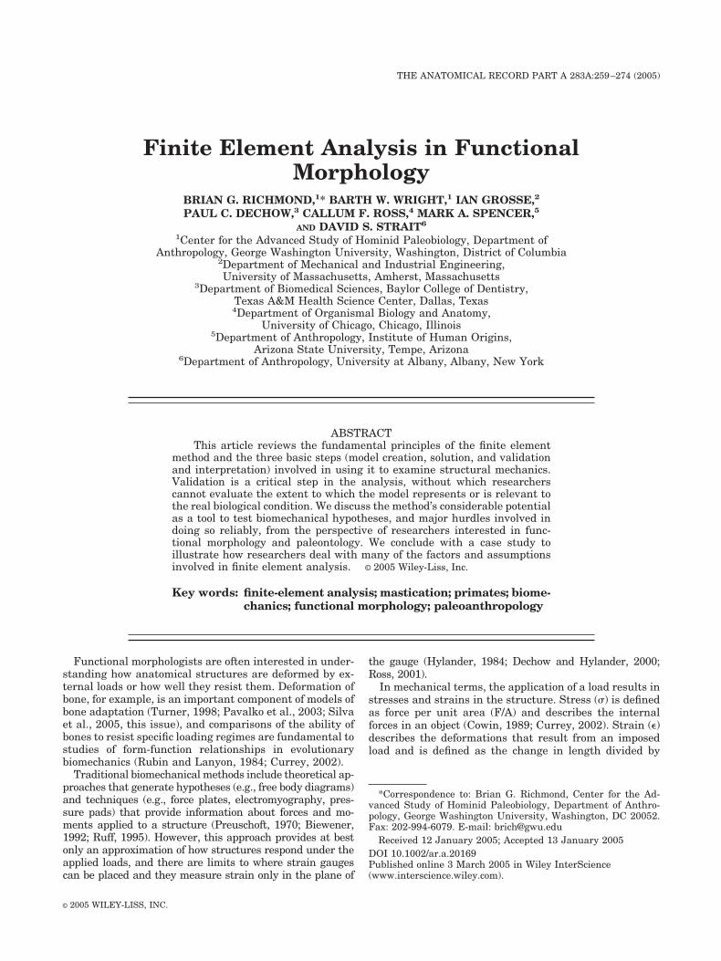
Stress and strain may be solved exactly by analyticalmeans for simple geometric shapes with homogeneousmaterial properties (Fig. 1). More complex problems arecomputationally impractical or intractable (Beaupre andCarter, 1992). Even a simple geometry (Fig. 1) cannot besolved analytically if the material properties or loadingconditions are complex, as is typically the case with bio-logical structures. The finite element method (FEM) pro-vides an approximate solution to such problems by subdi-viding the complex geometry into a finite (but typicallyhigh) number of elements of simple geometry (Fig. 1).

FEM was first developed as a mathematical techniqueas early as 1943 (Courant, 1943), but did not see wide-spread use until the advent of computers. Without com-puters, FEM was highly impractical and remained ig-nored until engineers, especially in the aerospaceindustry, independently developed it later (Levy, 1953).The use of FEM has dramatically increased in the fields ofengineering and biomechanics (Huiskes and Chao, 1983).Cook et al. (2001) note that 10 papers using finite ele-ments were published in 1961, 134 in 1966, and 844 in1971. In 1995, Mackerle (1995) estimated that over 56,000papers had been published on finite element analysis(FEA), hundreds of books and conference proceedings, aswell as the development of 310 general purpose finiteelement (FE) computer programs. FEM has also becomemore widely used in the life sciences. A search of theliterature in the National Library of Medicine’s PubMeddatabase identifies 1 finite-element paper in 1973, 29 in1983, 91 in 1993, and 457 in 2003.

Although FEA is a powerful tool and growing in popu-larity, it is important to remember that it is merely a tool.Before considering the best FEM approach, researchersshould first decide whether FE modeling is the bestmethod for testing the research questions. Once functionalmorphologists select FEA, they are faced with numerousdecisions about how best to employ it.

Before considering the method’s details, we offer defini-tions of several key terms. The terms “FEM” and “FEA”are often used interchangeably. FEM can be considered

the methodology in which the analysis of interest is con-verted into a set of algebraic simultaneous equations,whereas FEA refers to the process of analyzing the set ofequations. This distinction has little practical impact onthose using FEA to examine biological problems, as bothprocesses are embedded in commercial software tools.

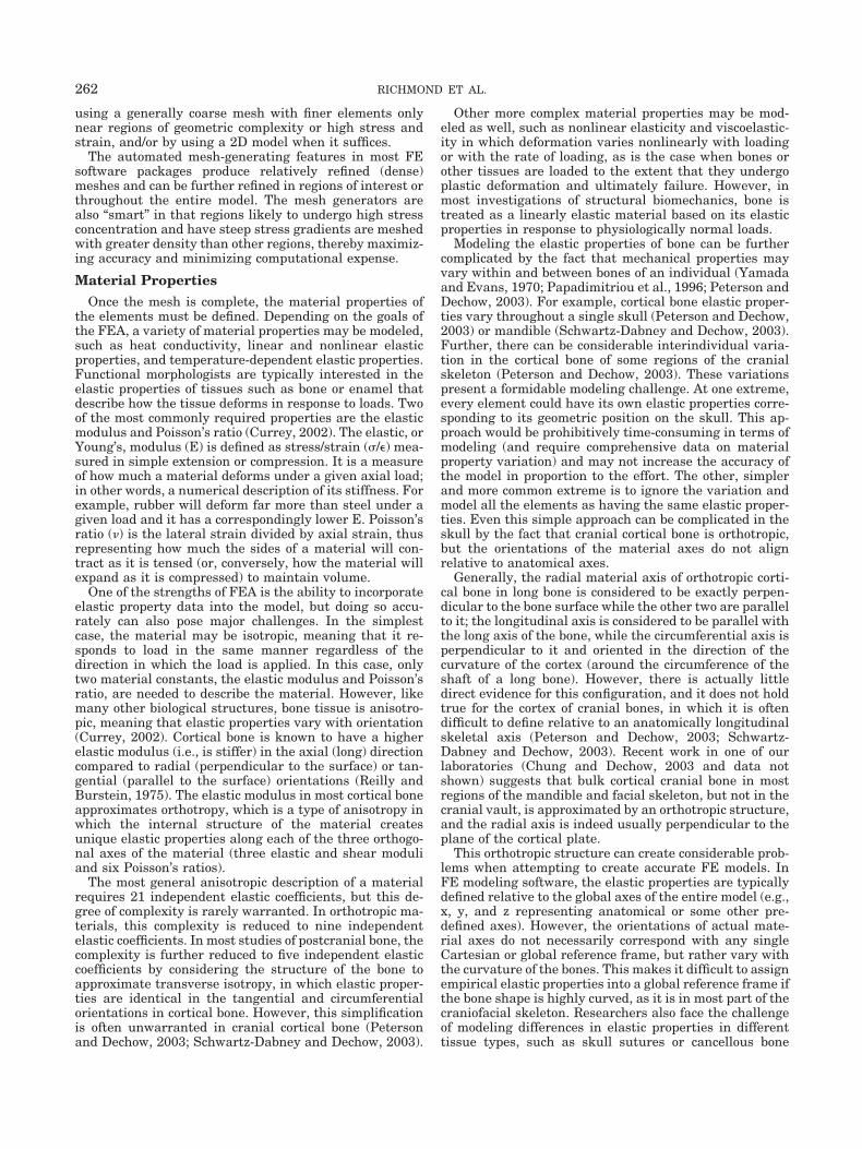
The term “FE modeling” refers to the process of creatingthe model, solving the model, and validating and inter-preting the results in the appropriate contexts. In thecontexts of functional morphology, creating the model istypically the most time-intensive phase. It involves col-lecting or integrating data or making assumptions aboutthe model’s geometry, mesh and element design, materialproperties, applied loads, and boundary conditions. Thesolution phase consists of calculating the stresses andstrains that result from the data and assumptions in themodel. The last phase, often called the postprocessingphase, involves the interpretation of the results. For bio-logical problems, validation is usually a very importantpart of this last phase because any interpretations madefrom the model’s results are dependent on the degree towhich the model reflects biological reality. Currently,most FEA papers in functional morphology include or citedata that form the bases of modeling decisions (e.g., ge-ometry, material properties, loads, and boundary condi-tions), but do not provide sufficient evidence to validatetheir model. Below, we discuss some of the major issuesand approaches involved in the three major steps, modelcreation, solution, and validation and interpretation, ofFE modeling (Fig. 2).

MODEL CREATIONGeometry

The first step in creating an FE model is deciding on thedimension (1-, 2-, or 3D) of the problem. Higher dimen-sions, while potentially more realistic, are disproportion-ately more difficult to model, solve, and subsequently ex-amine, and 2D analyses are often adequate for thequestions at hand (Richmond, 1998; Rayfield, 2004). Theresearcher must also decide on the geometric precisionneeded to address the questions of interest. Abstract geo-metric representations are relatively simple to create us-ing computer-automated design (CAD) software. Simplegeometric abstractions of real biological structures limitthe model’s potential and, if too abstract, may not be avalid representation of the real structure’s behavior.

To create a realistic geometric model, the geometry ofthe structure must be input into a computer. A variety oftechniques are available, including automated and man-ual techniques. One automated approach involves trans-forming laser scans of bones or other structures into wire-frame models that are then converted into FE models.Laser scans can offer a high-resolution representation ofthe outer surface, but lack information about internalgeometry (Kappelman, 1998). Computed tomography (CT)scan voxels (3D version of pixels, the unit volume resolu-tion) can also be directly transformed into the elements ofa high-resolution FE model (Ryan and van Rietbergen,2005). The automation and high resolution make thismethod attractive, but it also involves complex issues infinding appropriate thresholding algorithms to demarcatethe bone-air (or other) boundary reliably throughout astructure (e.g., skull) with varying bone thickness anddensity (Fajardo et al., 2002; Ryan and van Rietbergen,2005). It also currently results in models with so many

Fig. 1. Problems with simple geometry (left) may easily be solved.More complex shapes (center) are impractical or impossible to solveanalytically. The problem may be approximated (right) by subdividing thecomplex geometry into small elements of simple geometry.

260 RICHMOND ET AL.

elements that the models may require computational abil-ities beyond those available in many powerful desktopworkstations.

Images (e.g., photos, CT, MRI) can be manually digi-tized and made into CAD or other models that FE soft-ware can then mesh into FE models. Manual digitizationgives the researcher better control over the creation of themodel geometry, but involves other thresholding issues(e.g., consistently identifying the bone-air boundary) andcan be very time-consuming. We recommend againstbuilding 3D models based only on external morphology(e.g., with current laser scanning techniques) in mostcases because of the importance of internal structure onthe structure’s behavior. The researcher’s choice of auto-mated versus manual techniques will depend on the re-searcher’s goals and structure of interest.

MeshTransforming the geometry of the physical structure

(domain) into an FE model involves subdividing it into afinite, but usually large, number of geometrically simpledomains, called finite elements, connected together at

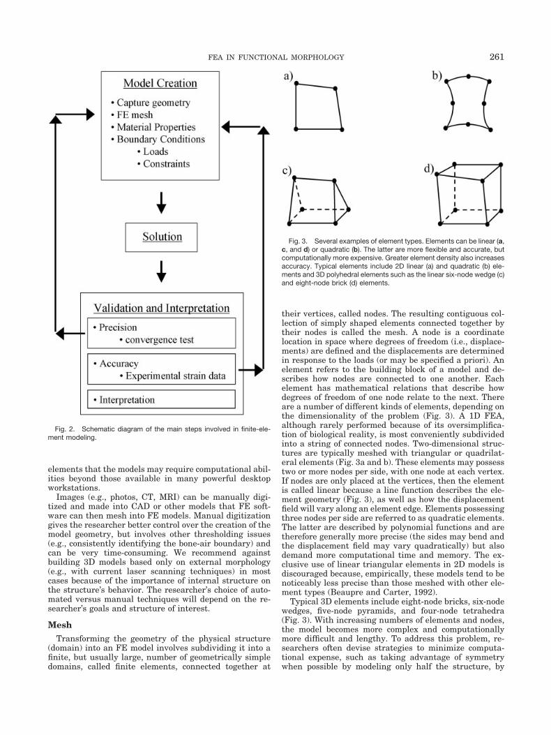
their vertices, called nodes. The resulting contiguous col-lection of simply shaped elements connected together bytheir nodes is called the mesh. A node is a coordinatelocation in space where degrees of freedom (i.e., displace-ments) are defined and the displacements are determinedin response to the loads (or may be specified a priori). Anelement refers to the building block of a model and de-scribes how nodes are connected to one another. Eachelement has mathematical relations that describe howdegrees of freedom of one node relate to the next. Thereare a number of different kinds of elements, depending onthe dimensionality of the problem (Fig. 3). A 1D FEA,although rarely performed because of its oversimplifica-tion of biological reality, is most conveniently subdividedinto a string of connected nodes. Two-dimensional struc-tures are typically meshed with triangular or quadrilat-eral elements (Fig. 3a and b). These elements may possesstwo or more nodes per side, with one node at each vertex.If nodes are only placed at the vertices, then the elementis called linear because a line function describes the ele-ment geometry (Fig. 3), as well as how the displacementfield will vary along an element edge. Elements possessingthree nodes per side are referred to as quadratic elements.The latter are described by polynomial functions and aretherefore generally more precise (the sides may bend andthe displacement field may vary quadratically) but alsodemand more computational time and memory. The ex-clusive use of linear triangular elements in 2D models isdiscouraged because, empirically, these models tend to benoticeably less precise than those meshed with other ele-ment types (Beaupre and Carter, 1992).

Typical 3D elements include eight-node bricks, six-nodewedges, five-node pyramids, and four-node tetrahedra(Fig. 3). With increasing numbers of elements and nodes,the model becomes more complex and computationallymore difficult and lengthy. To address this problem, re-searchers often devise strategies to minimize computa-tional expense, such as taking advantage of symmetrywhen possible by modeling only half the structure, by

Fig. 2. Schematic diagram of the main steps involved in finite-ele-ment modeling.

Fig. 3. Several examples of element types. Elements can be linear (a,c, and d) or quadratic (b). The latter are more flexible and accurate, butcomputationally more expensive. Greater element density also increasesaccuracy. Typical elements include 2D linear (a) and quadratic (b) ele-ments and 3D polyhedral elements such as the linear six-node wedge (c)and eight-node brick (d) elements.

261FEA IN FUNCTIONAL MORPHOLOGY

using a generally coarse mesh with finer elements onlynear regions of geometric complexity or high stress andstrain, and/or by using a 2D model when it suffices.

The automated mesh-generating features in most FEsoftware packages produce relatively refined (dense)meshes and can be further refined in regions of interest orthroughout the entire model. The mesh generators arealso “smart” in that regions likely to undergo high stressconcentration and have steep stress gradients are meshedwith greater density than other regions, thereby maximiz-ing accuracy and minimizing computational expense.

Material PropertiesOnce the mesh is complete, the material properties of

the elements must be defined. Depending on the goals ofthe FEA, a variety of material properties may be modeled,such as heat conductivity, linear and nonlinear elasticproperties, and temperature-dependent elastic properties.Functional morphologists are typically interested in theelastic properties of tissues such as bone or enamel thatdescribe how the tissue deforms in response to loads. Twoof the most commonly required properties are the elasticmodulus and Poisson’s ratio (Currey, 2002). The elastic, orYoung’s, modulus (E) is defined as stress/strain (�/�) mea-sured in simple extension or compression. It is a measureof how much a material deforms under a given axial load;in other words, a numerical description of its stiffness. Forexample, rubber will deform far more than steel under agiven load and it has a correspondingly lower E. Poisson’sratio (�) is the lateral strain divided by axial strain, thusrepresenting how much the sides of a material will con-tract as it is tensed (or, conversely, how the material willexpand as it is compressed) to maintain volume.

One of the strengths of FEA is the ability to incorporateelastic property data into the model, but doing so accu-rately can also pose major challenges. In the simplestcase, the material may be isotropic, meaning that it re-sponds to load in the same manner regardless of thedirection in which the load is applied. In this case, onlytwo material constants, the elastic modulus and Poisson’sratio, are needed to describe the material. However, likemany other biological structures, bone tissue is anisotro-pic, meaning that elastic properties vary with orientation(Currey, 2002). Cortical bone is known to have a higherelastic modulus (i.e., is stiffer) in the axial (long) directioncompared to radial (perpendicular to the surface) or tan-gential (parallel to the surface) orientations (Reilly andBurstein, 1975). The elastic modulus in most cortical boneapproximates orthotropy, which is a type of anisotropy inwhich the internal structure of the material createsunique elastic properties along each of the three orthogo-nal axes of the material (three elastic and shear moduliand six Poisson’s ratios).

The most general anisotropic description of a materialrequires 21 independent elastic coefficients, but this de-gree of complexity is rarely warranted. In orthotropic ma-terials, this complexity is reduced to nine independentelastic coefficients. In most studies of postcranial bone, thecomplexity is further reduced to five independent elasticcoefficients by considering the structure of the bone toapproximate transverse isotropy, in which elastic proper-ties are identical in the tangential and circumferentialorientations in cortical bone. However, this simplificationis often unwarranted in cranial cortical bone (Petersonand Dechow, 2003; Schwartz-Dabney and Dechow, 2003).

Other more complex material properties may be mod-eled as well, such as nonlinear elasticity and viscoelastic-ity in which deformation varies nonlinearly with loadingor with the rate of loading, as is the case when bones orother tissues are loaded to the extent that they undergoplastic deformation and ultimately failure. However, inmost investigations of structural biomechanics, bone istreated as a linearly elastic material based on its elasticproperties in response to physiologically normal loads.

Modeling the elastic properties of bone can be furthercomplicated by the fact that mechanical properties mayvary within and between bones of an individual (Yamadaand Evans, 1970; Papadimitriou et al., 1996; Peterson andDechow, 2003). For example, cortical bone elastic proper-ties vary throughout a single skull (Peterson and Dechow,2003) or mandible (Schwartz-Dabney and Dechow, 2003).Further, there can be considerable interindividual varia-tion in the cortical bone of some regions of the cranialskeleton (Peterson and Dechow, 2003). These variationspresent a formidable modeling challenge. At one extreme,every element could have its own elastic properties corre-sponding to its geometric position on the skull. This ap-proach would be prohibitively time-consuming in terms ofmodeling (and require comprehensive data on materialproperty variation) and may not increase the accuracy ofthe model in proportion to the effort. The other, simplerand more common extreme is to ignore the variation andmodel all the elements as having the same elastic proper-ties. Even this simple approach can be complicated in theskull by the fact that cranial cortical bone is orthotropic,but the orientations of the material axes do not alignrelative to anatomical axes.

Generally, the radial material axis of orthotropic corti-cal bone in long bone is considered to be exactly perpen-dicular to the bone surface while the other two are parallelto it; the longitudinal axis is considered to be parallel withthe long axis of the bone, while the circumferential axis isperpendicular to it and oriented in the direction of thecurvature of the cortex (around the circumference of theshaft of a long bone). However, there is actually littledirect evidence for this configuration, and it does not holdtrue for the cortex of cranial bones, in which it is oftendifficult to define relative to an anatomically longitudinalskeletal axis (Peterson and Dechow, 2003; Schwartz-Dabney and Dechow, 2003). Recent work in one of ourlaboratories (Chung and Dechow, 2003 and data notshown) suggests that bulk cortical cranial bone in mostregions of the mandible and facial skeleton, but not in thecranial vault, is approximated by an orthotropic structure,and the radial axis is indeed usually perpendicular to theplane of the cortical plate.

This orthotropic structure can create considerable prob-lems when attempting to create accurate FE models. InFE modeling software, the elastic properties are typicallydefined relative to the global axes of the entire model (e.g.,x, y, and z representing anatomical or some other pre-defined axes). However, the orientations of actual mate-rial axes do not necessarily correspond with any singleCartesian or global reference frame, but rather vary withthe curvature of the bones. This makes it difficult to assignempirical elastic properties into a global reference frame ifthe bone shape is highly curved, as it is in most part of thecraniofacial skeleton. Researchers also face the challengeof modeling differences in elastic properties in differenttissue types, such as skull sutures or cancellous bone

262 RICHMOND ET AL.

regions (Herring and Teng, 2000). More research isneeded to assess the impact of various simplifications ofthe complex variation found in the elastic properties ofsome skeletal elements on the reliability of associated FEmodels. Initial studies by our group (Strait et al., 2005,this issue) found that incorporating variation in elasticproperties across regions of the skull significantly im-proved the validation of a cranial FE model against exper-imental data.

After the elastic properties are defined, the elements areassembled into a global stiffness matrix [K]. Here theconnections between elements and nodes are definedwithin the model’s global framework in the form of {F} �[K]{D}. The geometry of each element is completely de-scribed by the list of nodes of which it is comprised andthis is referred to as the element connectivity (Hart, 1989).The element coordinate system (x-, y-, and z-coordinates ofeach element) is defined relative to a global frame ofreference (X-, Y-, and Z-axes of the entire model).

Boundary ConditionsThere are two types of boundary conditions. The kine-

matic or essential boundary conditions (see Appendix) aredisplacement constraints that prevent rigid movement ofthe model; the boundary constraints in effect anchor themodel. The natural or nonessential boundary conditionsinclude the loading conditions (e.g., forces) applied to themodel. Some researchers use the term “boundary condi-tions” to refer specifically to the essential constraints. Werefer to these essential boundary conditions as boundaryor displacement constraints, and the nonessential ones asloading conditions.

Boundary constraints are necessary because althoughthe external forces may be carefully calculated such thatthe model should be in equilibrium, it is virtually impos-sible to ensure that the forces are in perfect equilibrium(i.e., vectors collectively sum to zero) when applied to themodel. If the forces were not in perfect equilibrium, themodel would “move.” Moreover, without boundary con-straints, there are an infinite number of solutions to theproblem. The entire model can be uniformly displaced(moved) in the frame of reference as a rigid body withoutaffecting the elastic response of the structure. Therefore,the boundary constraints anchor the model and enable aunique elasticity solution to be obtained. Without bound-ary constraints, the FE computations will not be possible.

The boundary constraints may have a significant impacton model solution and must be chosen carefully. For ex-ample, nodes at one or more locations of ligament attach-ment sites might be selected as the location(s) to constrainthe model from translation or rotation (Richmond, 1998).One might constrain nodes at the location of a reactionforce (e.g., the bite point) rather than input an estimatedreaction force (e.g., resulting from the masticatory muscleforces). This will in effect apply the necessary reactionforce at that location.

Depending on the element types, specific nodes may bemodeled with any combination of constraints from trans-lation in, or rotation about, any axis direction (x, y, and z).Thus, constraints include six possible variables, althoughsolid elements typically only allow translational con-straints (these elements do not have rotational degrees offreedom). At a minimum, the model must be constrainedin some manner from translation in all three directions.Three-dimensional models must have sufficient boundary

constraints to prevent all six possible modes of rigid bodymotion. Although it is possible to constrain the entiremodel at a few nodes, this typically results in an unreal-istic condition in which very high strains and stresses arelocalized around the constrained node. In general, con-straints should be placed away from the primary region ofinterest because of potential local effects. Slight inaccura-cies in modeling the constraints are likely to influence thestrains and stresses adjacent to the constraints, but havelittle to no effect on regions more distant to the con-strained nodes (Cook et al., 2001).

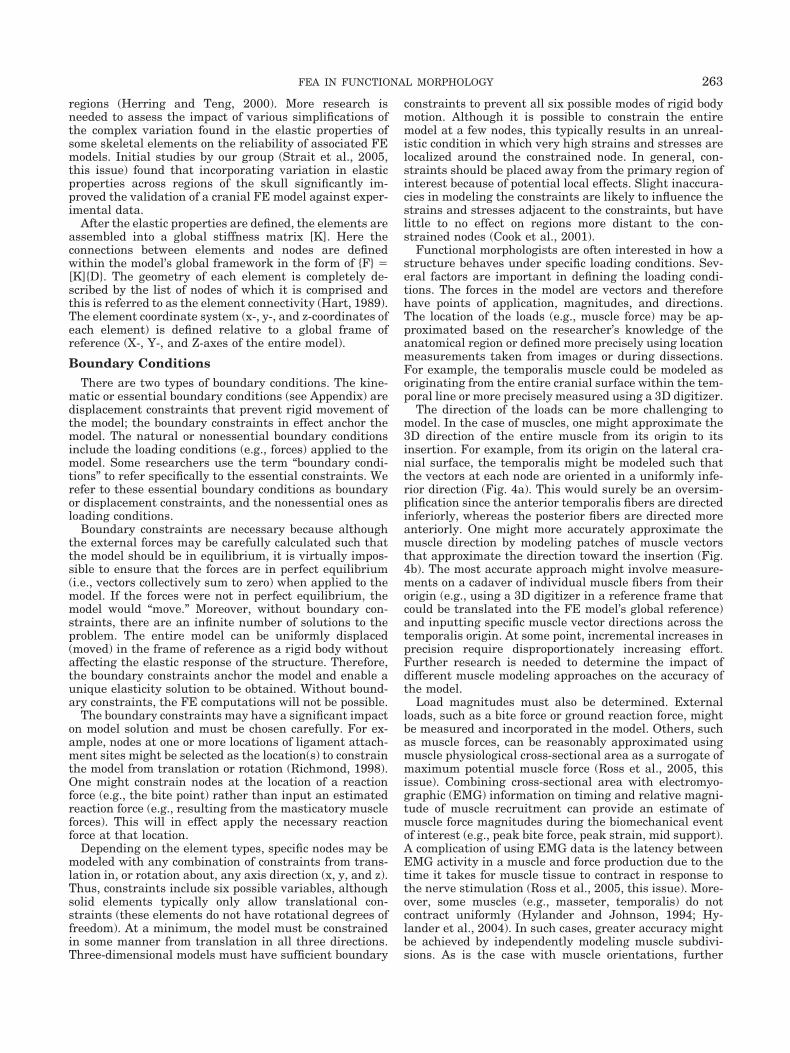
Functional morphologists are often interested in how astructure behaves under specific loading conditions. Sev-eral factors are important in defining the loading condi-tions. The forces in the model are vectors and thereforehave points of application, magnitudes, and directions.The location of the loads (e.g., muscle force) may be ap-proximated based on the researcher’s knowledge of theanatomical region or defined more precisely using locationmeasurements taken from images or during dissections.For example, the temporalis muscle could be modeled asoriginating from the entire cranial surface within the tem-poral line or more precisely measured using a 3D digitizer.

The direction of the loads can be more challenging tomodel. In the case of muscles, one might approximate the3D direction of the entire muscle from its origin to itsinsertion. For example, from its origin on the lateral cra-nial surface, the temporalis might be modeled such thatthe vectors at each node are oriented in a uniformly infe-rior direction (Fig. 4a). This would surely be an oversim-plification since the anterior temporalis fibers are directedinferiorly, whereas the posterior fibers are directed moreanteriorly. One might more accurately approximate themuscle direction by modeling patches of muscle vectorsthat approximate the direction toward the insertion (Fig.4b). The most accurate approach might involve measure-ments on a cadaver of individual muscle fibers from theirorigin (e.g., using a 3D digitizer in a reference frame thatcould be translated into the FE model’s global reference)and inputting specific muscle vector directions across thetemporalis origin. At some point, incremental increases inprecision require disproportionately increasing effort.Further research is needed to determine the impact ofdifferent muscle modeling approaches on the accuracy ofthe model.

Load magnitudes must also be determined. Externalloads, such as a bite force or ground reaction force, mightbe measured and incorporated in the model. Others, suchas muscle forces, can be reasonably approximated usingmuscle physiological cross-sectional area as a surrogate ofmaximum potential muscle force (Ross et al., 2005, thisissue). Combining cross-sectional area with electromyo-graphic (EMG) information on timing and relative magni-tude of muscle recruitment can provide an estimate ofmuscle force magnitudes during the biomechanical eventof interest (e.g., peak bite force, peak strain, mid support).A complication of using EMG data is the latency betweenEMG activity in a muscle and force production due to thetime it takes for muscle tissue to contract in response tothe nerve stimulation (Ross et al., 2005, this issue). More-over, some muscles (e.g., masseter, temporalis) do notcontract uniformly (Hylander and Johnson, 1994; Hy-lander et al., 2004). In such cases, greater accuracy mightbe achieved by independently modeling muscle subdivi-sions. As is the case with muscle orientations, further

263FEA IN FUNCTIONAL MORPHOLOGY

research is needed on muscle and other load magnitudesto assess the impact of modeling precision on the ultimatevalidity of the model.

SOLUTIONThe completed model is solved to obtain the nodal dis-

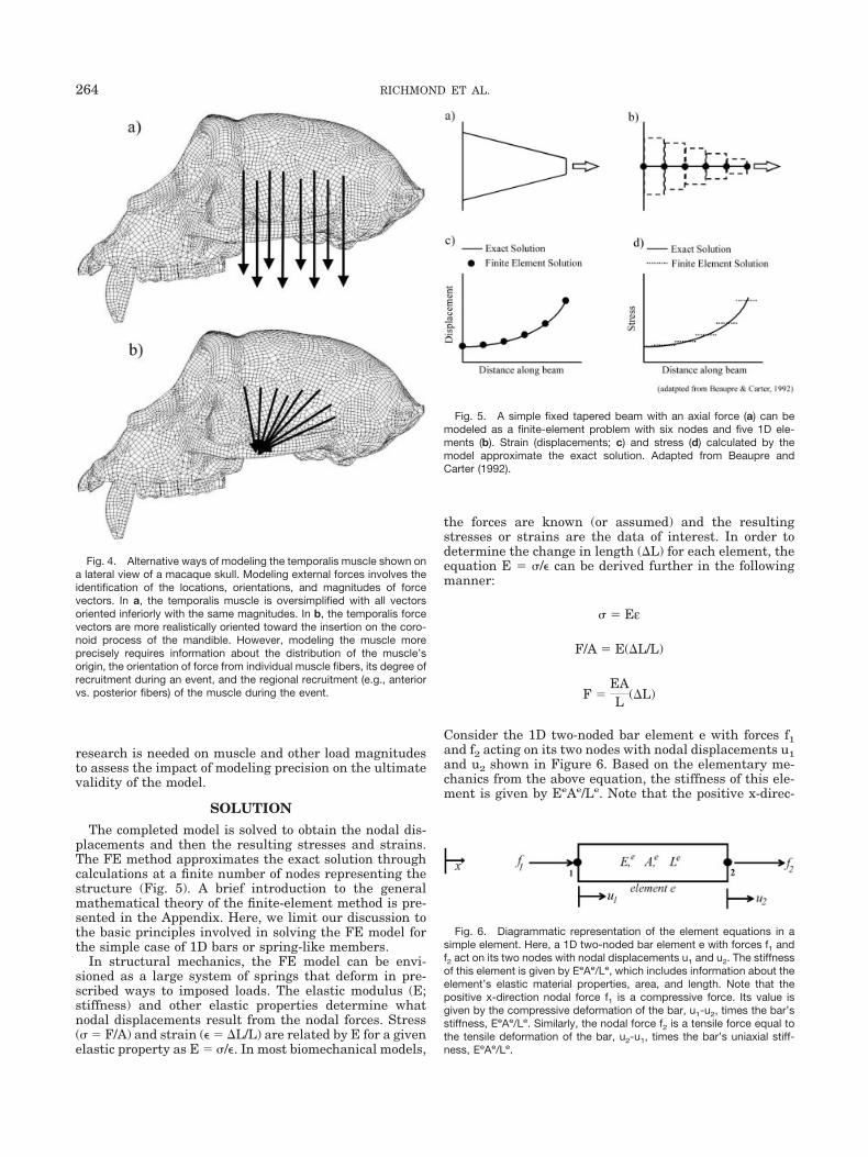
placements and then the resulting stresses and strains.The FE method approximates the exact solution throughcalculations at a finite number of nodes representing thestructure (Fig. 5). A brief introduction to the generalmathematical theory of the finite-element method is pre-sented in the Appendix. Here, we limit our discussion tothe basic principles involved in solving the FE model forthe simple case of 1D bars or spring-like members.

In structural mechanics, the FE model can be envi-sioned as a large system of springs that deform in pre-scribed ways to imposed loads. The elastic modulus (E;stiffness) and other elastic properties determine whatnodal displacements result from the nodal forces. Stress(� � F/A) and strain (� � �L/L) are related by E for a givenelastic property as E � �/�. In most biomechanical models,

the forces are known (or assumed) and the resultingstresses or strains are the data of interest. In order todetermine the change in length (�L) for each element, theequation E � �/� can be derived further in the followingmanner:

� � Eε

F/A � E(�L/L)

F �EAL (�L)

Consider the 1D two-noded bar element e with forces f1and f2 acting on its two nodes with nodal displacements u1and u2 shown in Figure 6. Based on the elementary me-chanics from the above equation, the stiffness of this ele-ment is given by EeAe/Le. Note that the positive x-direc-

Fig. 6. Diagrammatic representation of the element equations in asimple element. Here, a 1D two-noded bar element e with forces f1 andf2 act on its two nodes with nodal displacements u1 and u2. The stiffnessof this element is given by EeAe/Le, which includes information about theelement’s elastic material properties, area, and length. Note that thepositive x-direction nodal force f1 is a compressive force. Its value isgiven by the compressive deformation of the bar, u1-u2, times the bar’sstiffness, EeAe/Le. Similarly, the nodal force f2 is a tensile force equal tothe tensile deformation of the bar, u2-u1, times the bar’s uniaxial stiff-ness, EeAe/Le.

Fig. 4. Alternative ways of modeling the temporalis muscle shown ona lateral view of a macaque skull. Modeling external forces involves theidentification of the locations, orientations, and magnitudes of forcevectors. In a, the temporalis muscle is oversimplified with all vectorsoriented inferiorly with the same magnitudes. In b, the temporalis forcevectors are more realistically oriented toward the insertion on the coro-noid process of the mandible. However, modeling the muscle moreprecisely requires information about the distribution of the muscle’sorigin, the orientation of force from individual muscle fibers, its degree ofrecruitment during an event, and the regional recruitment (e.g., anteriorvs. posterior fibers) of the muscle during the event.

Fig. 5. A simple fixed tapered beam with an axial force (a) can bemodeled as a finite-element problem with six nodes and five 1D ele-ments (b). Strain (displacements; c) and stress (d) calculated by themodel approximate the exact solution. Adapted from Beaupre andCarter (1992).

264 RICHMOND ET AL.

tion nodal force f1, as illustrated in Figure 6, is acompressive force. Its value is given by the compressivedeformation of the bar, u1-u2, times the bar’s stiffness,EeAe/Le. Similarly, an assumed positive nodal force f2 is atensile force equal to the tensile deformation of the bar,u2-u1, times the bar’s uniaxial stiffness, EeAe/Le. Thus,

f1 �EeAe

Le (u1 � u2)

f2 �EeAe

Le (u2 � u1)

In matrix notation, the above element equations are ex-pressed as

{f} � [Ke]{d}

[Ke] �EeAe

Le � 1 �1�1 1 �

Due to the connection of elements together by sharednodes, the individual element equations are assembledinto a set of simultaneous algebraic equations that relatesall the nodal displacements to nodal forces via the systemstiffness matrix:

{F} � [K]{D}

where {F} is the vector of nodal forces (the loads applied tothe model), [K] is referred to as the system stiffness ma-trix because it contains information about elastic proper-ties and geometry, and {D} is the vector of nodal displace-ments (i.e., the �L values). Therefore, the external forces{F} and mechanical properties and geometry [K] are usedto calculate the displacements {D} at each node (Cook etal., 2001). Once nodal displacements are known, the dis-placement field is interpolated from nodal values usingstandard interpolating polynomial functions. If the ele-ment is linear, then the interpolating polynomial is linear.Differentiation of the displacement field yields the straindistribution. The stress distribution is then obtained us-ing the elastic property or constitutive relations (e.g., E ��/�), which relate strains (�) to stresses (�).

In the FE method, the theoretically exact stress tensorin equilibrium equations is replaced with an approximateone (the FEM stress tensor), resulting in a residual orerror function that is a function of spatial coordinates andunknown parameters in our FEA formulation (nodal de-grees of freedom). Similarly, boundary equilibrium equa-tions are no longer satisfied when an approximate solutionis used, yielding a boundary residual or error function.Using a mathematical approach known as Galerkin’smethod of weighted residuals (see Appendix), the FEMforces the domain and boundary residual functions to bezero (orthogonal to the weighting functions; see Appendixfor more details). With this approach, as the mesh isrefined, the error functions must come closer and closer tothe zero function. Since only the exact solution completelysatisfies the domain and boundary equilibrium equations,the finite-element solution must converge to the theoreti-

cal exact solution. This approach ensures that the discreti-zation error (the error involved in replacing a continuousstructure with a finite number of elements) can be reliablydecreased with increasing element density. In otherwords, as the number of nodes increases, the precision ofthe model increases. Empirically, the approximations tendto match closely the exact solution when it can be calcu-lated (Fig. 5).

VALIDATION AND INTERPRETATIONNo matter how much thought and research goes into

model creation, the results may be wrong. For biologicalproblems, researchers should be able to address both theprecision and accuracy of the model (Huiskes and Chao,1983). Accuracy is defined here as the closeness of themodel’s results to the real biological situation. Precision isdefined here as the closeness of the model’s results to theexact solution of that biomechanical model. Various termsare used in the literature to describe these types of valid-ity. Our definitions of the terms “accuracy” and “precision”reflect their use in statistics and other fields, but corre-spond with Huiskes and Chao’s (1983) terms “validity”and “accuracy,” respectively.

In this sense, precision is similar to its use in statistics,where it relates to the number of significant figures re-corded for measurements (Sokal and Rohlf, 1995). A modelwould be precise but inaccurate if the mesh is very densebut the loading and boundary conditions are unrealistic.Precision and accuracy require different kinds of valida-tion.

The precision of a particular FE model can be assessedthrough a convergence test in which the model is repeat-edly calculated with increasingly finer meshes until thedisplacement magnitude of a chosen test area reaches aplateau, converging toward a precise solution of thatmodel (Hart, 1989). In the past, assessing precision wasan important step because limitations on computer powerrequired researchers to determine an appropriate degreeof mesh refinement that was reasonably precise but min-imized computational demand. This has become less of anissue with more powerful computers that allow programsautomatically to generate meshes that typically have am-ple density and increase mesh density in regions likely toundergo high stress concentrations. However, the onlyway to assess discretization error is to conduct a conver-gence test in which specific analytic quantities (e.g., max-imum principal strain) at specific locations are comparedbetween three or more meshes of different refinement.

No matter how finely the structure is meshed and howprecisely the calculations are performed, the computedanswer may still be wrong (Cook et al., 2001). Indepen-dent experimental support is critical to any FEA attempt-ing to model a mechanical problem in a realistic manner.The best means of validation involves the direct measure-ment of strain, as in in vivo strain gauge experiments(Rubin and Lanyon, 1982; Hylander and Johnson, 1992;Ross, 2001). Cadaver strain experiments are also usefuland provide greater control over biomechanical variables(Ross and Hylander, 1996; Richmond, 1998). A combina-tion of in vitro and in vivo experimentation potentiallyoffers the best validation. In vitro validation allows one tocarefully control the loads and boundary constraints inorder to assess the validity of the model’s geometry andelastic properties. Here, the controlled loading and bound-ary conditions can be put in the FE model and the FE

265FEA IN FUNCTIONAL MORPHOLOGY

results compared to the in vitro results. If necessary, themodel geometry and elastic properties can be altered tominimize the discrepancies between the model and empir-ical results. Once the geometry and elastic properties areadequately modeled, discrepancies between the model andin vivo results can be confidently attributed to the model’sloads and boundary constraints, and these can be refinedif the model does not accurately reflect the in vivo condi-tion.

Working from the other side of the analysis, experimen-tal work to determine the loading conditions and mechan-ical properties prior to modeling can also greatly improvethe model. While this cannot be considered validation,empirical data put into the model from the outset cangreatly improve the model’s accuracy.

As in other FE modeling steps, several issues complicatethe validation process. For example, the model and exper-imental data differ in some ways that affect attempts atvalidation. Published experimental data typically consistof peak strain values for a number of anatomical regions(Hylander and Johnson, 1997), although these regionsmay not experience peak strain simultaneously (Hylanderand Johnson, 1994; Ross, 2001). However, strains occursimultaneously in static FE models. A second exampleconcerns the fact that in vivo strain gauges measurestrain only in the plane of the gauge. Thus, the 3D strainorientations in the FE model must be projected into theplane of the gauge in order to compare them. A thirdcomplication is that published in vivo strain gauge loca-tions are unfortunately not reported with the precisionnecessary to make precise location comparisons betweenthe model and the experimental subjects. In regions ofhigh strain gradients such as the curved browridge, slightdifferences in location can make a large difference instrain magnitude and orientation. Greater precision inreporting anatomical locations of gauges during in vivostrain experiments would be an improvement. A finalissue, and probably the most difficult one, is the questionover the level of correspondence between the model andthe in vivo evidence that must be reached before the modelcan be considered valid. The answer depends on the hy-potheses and goals of the study. Some may require accu-racy in absolute strain values, while others may onlyrequire that the model deforms in a broadly similar way tothe real biological structure.

Some researchers have taken the approach of buildingabstract representations of a structure (Witzel andPreuschoft, 1999; Jenkins et al., 2002; Witzel et al., 2004).Here, researchers are attempting to model, in a tradi-tional sense of the term, a complex system as a simplifiedabstraction. This approach has its merits. If successful,much can be learned about the biomechanical problem ina straightforward manner. However, researchers must bevery careful to consider the limits of a simplified model ifthey intend to make adaptive or behavioral inferencesfrom the model’s results. Validation of the positive andnegative aspects of such a model can sometimes be formu-lated through creative experimentation. Without such at-tempts at validation, it is often difficult to evaluatewhether the results have any significance in the realworld. Unfortunately, most FEA studies to date in func-tional morphology literature or in the large clinical FEAliterature include little or no validation of their models(Spears and Crompton, 1996; Spears and Macho, 1998;Macho and Spears, 1999; Witzel and Preuschoft, 1999;

Rayfield et al., 2001; Witzel et al., 2004; Ryan and vanRietbergen, 2005).

Validation and model refinement can be repeated untilthe two converge. Near perfect validity can become veryexpensive in use of time and resources and may be exces-sive depending on the question of interest. An FE model is,after all, a model. The researcher must decide how accu-rate is accurate enough, but should have some evidence onwhich to base this decision.

After validating the model, the researcher may begin tointerpret the results. As in any study, the results shouldobviously be interpreted in the context of the questionsforming the bases of the analysis. The vast quantities ofdata generated in an FEA pose challenges at this stage.Visualizing the results is an almost universal first step.Beyond this step are many strategies for illustrating andevaluating the results and assessing their statistical sig-nificance. Examples can be found in the literature (e.g.,Ross et al., 2005, this issue) and are beyond the scope ofthis review.

APPLICATIONSThere are at least three general applications of FEA in

functional morphology today. One is to develop realisticmodels of biological problems. This is the traditional ap-proach in biomechanics and orthopedics, in which individ-ual skeletal elements or joints, such as the proximal femur(Beaupre et al., 1990) or skull (Strait et al., 2005), aremodeled to better understand how the bones involvedbehave in response to applied loads. Independent valida-tion is most important in this kind of FEA.

Another, less frequent, use for FEA involves integratinginformation from multiple strain gauges to estimate shearstrains in a particular cross-section. When three or morerosette gauges record strain around the circumference of along bone, Rybicki et al.’s (1977) method can be used toestimate the position of the neutral axis of bending, thedistribution of strain due to bending throughout the cross-section, and maximum strain values in compression andtension (Carter et al., 1981; Gross et al., 1992; Roszek etal., 1993; Demes et al., 1998). However, in order to calcu-late shear strain, simplifying assumptions or FEA arenecessary (Fritton and Rubin, 2001).

A third category of applications for FEA in functionalmorphology is a comparative one. FEA may be used tocompare the mechanical behavior of different skeletal de-signs of the same structure (Richmond, 1998; Ryan andvan Rietbergen, 2005). In this way, FEA promises to be apowerful new tool for testing biomechanical hypotheses inextant and fossil taxa. Under similar loading conditions,the probable strain regime of a unique fossil shape may becompared to other fossil forms or related living forms. Inthis kind of analysis, it is important to have a good un-derstanding of the biomechanics of the problem in livingforms that are most closely related to the fossil taxa (Rud-wick, 1964; Lauder, 1995). If all related living taxa sharea similar biomechanical regime (e.g., same suite of mus-cles, attached in similar places), it is most likely that thefossil taxa did so too, despite differences in morphology. Insome cases, particularly those involving extinct taxa, itmay not be possible to collect some of the data that wouldimprove the model’s accuracy. In these situations, FEAcan be useful if the purpose of the analysis is not absoluteaccuracy but the relative abilities of structures to resistloading regimes.

266 RICHMOND ET AL.

FEA can also be used to examine the structural behav-ior of specific anatomical features, such as the zygomaticarch (Witzel et al., 2004) or palate thickness (Strait et al.,2005). FE methods provide controlled experimental condi-tions that allow researchers to isolate the mechanicalsignificance of a single morphological trait by comparingtwo organisms that differ only in that trait. FEA promisesto offer new insights into the mechanical significance ofnovel evolutionary structures, such as the hard palate,postorbital bar, and sutural fusion in the mandible andcranial bones. FEA also offers researchers a unique way toexamine the interactive mechanical effect of combinationsof features not present in extant or fossil taxa. Such an

approach might allow researchers to evaluate more accu-rately whether features in fossil taxa should be consideredas adaptations to particular functions.

An exciting new direction involves using FEA to inves-tigate biological processes. In a pioneering example of thisapproach, Beaupre et al. (1990) tested their remodelingtheory (e.g., the rules governing the remodeling process)by comparing real bone structure to the results of an FEmodel that was repeatedly loaded and altered followingthe rules of the theory. In this way, they were able toassess the utility of the remodeling theory and show thatsimilar stress-related phenomena might be responsible fornormal bone morphogenesis as well as functional adapta-

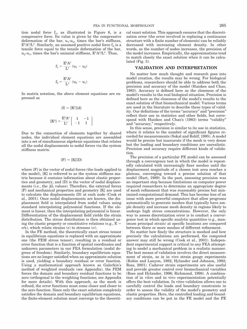
Fig. 7. An illustrative example of creating an FE mesh. a: The external then internal outlines of successiveCT scans of a macaque skull were digitized and linked using CAD software. The linked outlines wereconverted into a solid CAD model. b: The entire solid model of a macaque skull was converted into a 3D FEmesh of linear brick and other polyhedral elements.

267FEA IN FUNCTIONAL MORPHOLOGY

tion in response to altered loads (Beaupre et al., 1990). Inthis issue, Preuschoft and Witzel (2005), use FE modelingin a creative way to test hypotheses about potential evo-lutionary rules underlying skull morphology by applyingmuscle loads to a block with only minimal skull form(orbits, dental arcade, muscle origin locations) and com-paring the resulting stress distributions against real skullform. By iteratively removing low stress regions of theblock, they find that the reduced model is similar to thetrue skull form. These results have interesting implica-tions for the role of optimality in the evolution of skeletalmorphology. Iterative approaches like these promise tohelp elucidate the processes underlying the functionaladaptation and morphogenesis of biological tissues andpotentially the evolutionary changes in morphology inresponse to changes in lifestyle.

The case study below provides one example of how FEmodeling can be used to investigate specific adaptive hy-potheses in fossil taxa.

CASE STUDYThe human fossil record includes an impressive diver-

sity in craniofacial morphology (Stringer and Trinkaus,1981; Rak, 1983; Walker et al., 1986; Brunet et al., 2002;Brown et al., 2004; Kimbel et al., 2004). Not surprisingly,these fossils have generated much discussion aboutcraniofacial adaptations to biting and chewing. One fossilgroup in particular, the robust australopiths, displays asuite of derived craniofacial features and very large,thickly enameled molars and premolars (Grine, 1988).Researchers disagree on the specific suites of derivedtraits that they would consider adaptations to chewing, adisagreement that affects the reconstruction of their phy-logenetic relationships (e.g., different suites of integratedtraits) and paleobiology (Skelton and McHenry, 1998;Strait and Grine, 1998).

Our work on FE modeling of a macaque skull is aimed atbuilding accurate primate skull models to test functionaland evolutionary hypotheses and ultimately biomechani-cal hypotheses in fossil primate skulls. To help illustratehow FE modeling can be used to test such hypotheses, weexamined the biomechanical significance of one trait, pal-ate thickness, hypothesized to be an adaptation in robustaustralopithecines to increased masticatory stresses(Strait et al., 2005). We built a 3D model of a macaqueskull during static centric occlusion, validated it againstin vivo bone strain data, and altered the palate thicknessof the model to assess the mechanical significance of thisfeature. We outline the FE modeling process below.

Geometry and MeshThe complexity of the skull and decision to compare

strain at various points throughout the skulls of thick-and thin-palate FE models required a 3D model. Weselected Macaca fascicularis because of the in vivostrain data available for this taxon (Hylander et al.,1991a; Hylander and Johnson, 1997). We obtained CTscans of the skull and manually digitized the scans inSolidworks CAD modeling software to create a virtualsolid model including external and internal surfaces(Fig. 7). The models were aligned such that the occlusalplane was horizontal. The CAD wire-frame model wasthen imported into the FEA software ALGOR, and theautomated 3D mesh-generating feature was used to cre-

ate an FE mesh consisting of 145,480 polyhedral brickelements (the Normal Model). We then altered the ini-tial CAD model by artificially increasing the thicknessof the palate and converted it into a second FE mesh(Thick Model) consisting of 290,639 elements. A struc-ture as geometrically complex as the skull requires theautomatic mesh-generating software to make many de-cisions about local mesh densities that result in differ-ent total element numbers. Although the two modelsdiffered in element number, both exhibited high concen-

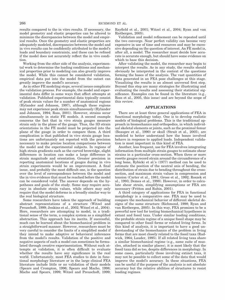
Fig. 8. The maximum principal strain orientations (and magnitudes;not shown) of the model are compared to the range of values observedfrom in vivo experiments of different macaque individuals. In six of theseven locations, the strain orientations lie within or adjacent to the in vivoresults, indicating that the model is reasonably valid in its representationof the manner of deformation. Note that the location in which the modeland experimental orientations differ is the highly curved zygomatic arch(working side). The steep strain gradients in this region leave open thepossibility that some of the discrepancy might be attributable to be-tween-individual morphological variation or lack of precision in identify-ing gauge location on the model. Model refinement and increased pre-cision in measuring gauge location during in vivo experiments thereforemight focus on this region.

268 RICHMOND ET AL.

trations of elements in regions that are likely to expe-rience high strain gradients, and independent experi-mental data support the validity of the Normal Model.

Material PropertiesElastic property data from 25 locations on macaque

skulls were used (data not shown). As a simplification,

bone was modeled isotropically, with the values of Young’smodulus (19.8 GPa) and Poisson’s ratio (0.315) represent-ing averages of the respective values in the axis of maxi-mum stiffness obtained at all locations on the face. In asubsequent analysis, we modeled anisotropic elastic prop-erties and properties in different regions (Strait et al.,2005, this issue).

Boundary ConditionsThe necessary boundary conditions included muscle

forces and external constraints to restrict translation androtation of the model. Eight muscle forces were applied tothe meshes corresponding to the primary jaw adductingmuscles: right and left anterior temporalis, superficialmasseter, deep masseter, and medial pterygoid muscles.Muscle orientations were estimated by measuring the po-

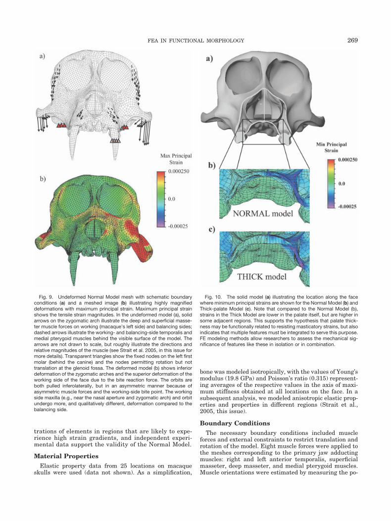
Fig. 9. Undeformed Normal Model mesh with schematic boundaryconditions (a) and a meshed image (b) illustrating highly magnifieddeformations with maximum principal strain. Maximum principal strainshows the tensile strain magnitudes. In the undeformed model (a), solidarrows on the zygomatic arch illustrate the deep and superficial masse-ter muscle forces on working (macaque’s left side) and balancing sides;dashed arrows illustrate the working- and balancing-side temporalis andmedial pterygoid muscles behind the visible surface of the model. Thearrows are not drawn to scale, but roughly illustrate the directions andrelative magnitudes of the muscle (see Strait et al. 2005, in this issue formore details). Transparent triangles show the fixed nodes on the left firstmolar (behind the canine) and the nodes permitting rotation but nottranslation at the glenoid fossa. The deformed model (b) shows inferiordeformation of the zygomatic arches and the superior deformation of theworking side of the face due to the bite reaction force. The orbits areboth pulled inferolaterally, but in an asymmetric manner because ofasymmetric muscle forces and the working-side bite point. The workingside maxilla (e.g., near the nasal aperture and zygomatic arch) and orbitundergo more, and qualitatively different, deformation compared to thebalancing side.

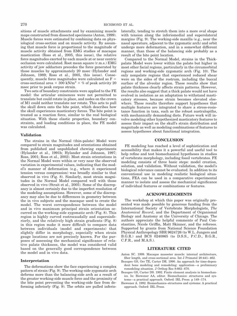
Fig. 10. The solid model (a) illustrating the location along the facewhere minimum principal strains are shown for the Normal Model (b) andThick-palate Model (c). Note that compared to the Normal Model (b),strains in the Thick Model are lower in the palate itself, but are higher insome adjacent regions. This supports the hypothesis that palate thick-ness may be functionally related to resisting masticatory strains, but alsoindicates that multiple features must be integrated to serve this purpose.FE modeling methods allow researchers to assess the mechanical sig-nificance of features like these in isolation or in combination.

269FEA IN FUNCTIONAL MORPHOLOGY

sitions of muscle attachments and by examining musclemaps constructed from dissected specimens (Anton, 1999).Muscle forces were estimated by combining data on phys-iological cross-section and on muscle activity. By assum-ing that muscle force is proportional to the magnitude ofmuscle activity obtained from EMG studies of macaquemastication (Ross et al., 2005, this issue), the relativeforce magnitudes exerted by each muscle at or near centricocclusion were calculated. Root mean square (r.m.s.) EMGactivity of jaw adductors precedes the force generated bythose muscles by approximately 20 msec (Hylander andJohnson, 1989; Ross et al., 2005, this issue). Conse-quently, muscle force magnitudes were calculated as F �cross-sectional area � 300 kN/m2 � % of peak activity 20msec prior to peak corpus strain.

Two sets of boundary constraints were applied to the FEmodel: the articular eminences were not permitted totranslate but could rotate in place, and nodes on the crownof M1 could neither translate nor rotate. This acts to pullthe skull down onto the bite point, which describes howthe skull experiences masticatory forces. The bite point istreated as a reaction force, similar to the real biologicalsituation. With these elastic properties, boundary con-straints, and loading conditions in place, the FE modelwas calculated.

ValidationThe strains in the Normal (thin-palate) Model were

compared to strain magnitudes and orientations obtainedfrom published and unpublished chewing experiments(Hylander et al., 1991b; Hylander and Johnson, 1997;Ross, 2001; Ross et al., 2002). Most strain orientations inthe Normal Model were within or very near the observedvariation in experimental values, indicating that the mod-el’s manner of deformation (e.g., where it experiencedtension versus compression) was broadly similar to thatobserved in vivo (Fig. 8). Similarly, most strain magni-tudes in the Normal Model compared well with thoseobserved in vivo (Strait et al., 2005). Some of the discrep-ancy is almost certainly due to the imperfect resolution ofthe modeling assumptions. However, some of the discrep-ancy may also be due to differences in geometry betweenthe in vivo subjects and the macaque used to create themodel. The worst correspondence between the modeland in vivo maximum principal strain orientation oc-curred on the working-side zygomatic arch (Fig. 8). Thisregion is highly curved rostrocaudally and superoinfe-riorly, and the relatively high strain gradients (Fig. 8)in this region make it more difficult to compare databetween individuals (model and experiments) thatslightly differ in morphology, especially when straingauge locations are not precisely known. For the pur-poses of assessing the mechanical significance of rela-tive palate thickness, the model was considered validbased on the generally good correspondence betweenthe model and in vivo data.

InterpretationThe deformations show the face experiencing a complex

pattern of strain (Fig. 9). The working-side zygomatic archdeforms more than the balancing-side arch as a result ofthe greater working-side muscle force and the proximity ofthe bite point preventing the working-side face from de-forming inferiorly (Fig. 9). The orbits are pulled inferio-

laterally, tending to stretch them into a more oval shapewith tension along the inferiomedial and superolateralmargins (Fig. 9). The working-side maxilla (e.g., near thenasal aperature, adjacent to the zygomatic arch) and orbitundergo more deformation, and in a somewhat differentmanner, than those of the balancing side probably as aresult of the bite point location.

Compared to the Normal Model, strains in the Thick-palate Model were lower within the palate but higher inmost other facial regions, particularly in the circumorbitalregions and working-side zygomatic arch (Fig. 10). Theonly nonpalate regions that experienced reduced shearwere on the sides of the rostrum, including the buccalsurface of the alveolar region. These results show thatpalate thickness clearly affects strain patterns. However,the results also suggest that a thick palate would not haveevolved in isolation as an adaptation to withstand masti-catory stresses, because strain becomes elevated else-where. These results therefore support hypotheses thatmultiple features are integrated to share a stress-resis-tance function in taxa, such as the robust australopiths,with mechanically demanding diets. Future work will in-volve modeling other hypothesized masticatory features toassess their impact on the skull’s strain distribution andmagnitude as well as modeling combinations of features toassess hypotheses about functional integration.

CONCLUSIONFE modeling has reached a level of sophistication and

accessibility that makes it a powerful and useful tool tohelp refine and test biomechanical hypotheses in studiesof vertebrate morphology, including fossil vertebrates. FEmodeling consists of three basic steps: model creation,solution, and validation. Without validation, the model’sbiological relevance cannot be evaluated. In addition to itsconventional use in modeling realistic biological situa-tions, FEA can be used in a comparative experimentalmanner to isolate and assess the mechanical significanceof individual features or combinations or features.

ACKNOWLEDGMENTSThe workshop at which this paper was originally pre-

sented was made possible by generous funding from theInternational Society of Vertebrate Morphologists, TheAnatomical Record, and the Department of OrganismalBiology and Anatomy at the University of Chicago. Theauthors appreciate the helpful comments of Paul Con-stantino, Nicole Griffin, Matt Skinner, and the referees.Supported by grants from National Science FoundationPhysical Anthropology SBR 9624726 (to W.L. Jungers andB.G.R.) and BCS 0240865 (to D.S.S., P.C.D., B.G.R.,C.F.R., and M.A.S.).

LITERATURE CITEDAnton SC. 1999. Macaque masseter muscle: internal architecture,

fiber length, and cross-sectional area. Int J Primatol 20:441–462.Beaupre GS, Orr TE, Carter DR. 1990. An approach for time-depen-

dent bone modeling and remodeling: application—a preliminaryremodeling situation. J Orthop Res 8:662–670.

Beaupre GS, Carter DS. 1992. Finite element analysis in biomechan-ics. In: Biewener AA, editor. Biomechanics: structures and sys-tems—a practical approach. Oxford: IRL Press. p 149–174.

Biewener A. 1992. Biomechanics–structures and systems: A practicalapproach. Oxford: IRL Press.

270 RICHMOND ET AL.

Brown P, Sutikna T, Morwood MJ, Soejono RP, Jatmiko, SaptomoEW, Due RA. 2004. A new small-bodied hominin from the LatePleistocene of Flores, Indonesia. Nature 431:1055–1061.

Brunet M, Guy F, Pilbeam D, Mackaye HT, Likius A, Ahounta D,Beauvilain A, Blondel C, Bocherens H, Boisserie JR, De Bonis L,Coppens Y, Dejax J, Denys C, Duringer P, Eisenmann V, Fanone G,Fronty P, Geraads D, Lehmann T, Lihoreau F, Louchart A, Maha-mat A, Merceron G, Mouchelin G, Otero O, Pelaez Campomanes P,Ponce De Leon M, Rage JC, Sapanet M, Schuster M, Sudre J, TassyP, Valentin X, Vignaud P, Viriot L, Zazzo A, Zollikofer C. 2002. Anew hominid from the Upper Miocene of Chad, Central Africa.Nature 418:145–151.

Carter DR, Harris W, Vasu R, Carter W. 1981. The mechanical andbiological response of cortical bone for in vivo strain histories. In:Cawin SC, editor. Mechanical properties of bone. New York: Amer-ican Society of Mechanical Engineers. p 81–92.

Chung DW, Dechow PC. 2003. Contrasts in off-axis ultrasonic velocitymeasurements in cortical bone from human crania and femur. JDent Res 82A:1509.

Cook RD, Malkus DS, Plesha ME, Witt RJ. 2001. Concepts andapplications of finite-element analysis, 4 ed. New York: John Wileyand Sons.

Courant R. 1943. Variation methods for the solution of problems ofequilirium and vibrations. Bull Am Math Soc 49:1–23.

Cowin SC. 1989. Mechanics of materials. In: Cowin SC, editor. Bonemechanics. Boca Raton: CRC Press. p 15–42.

Currey JD. 2002. Bones: structures and mechanics. Princeton, NJ:Princeton University Press.

Dechow PC, Hylander WL. 2000. Elastic properties and masticatorybone stress in the macaque mandible. Am J Phys Anthropol 112:553–574.

Demes B, Stern JT, Jr, Hausman MR, Larson SG, McLeod KJ, RubinCT. 1998. Patterns of strain in the macaque ulna during functionalactivity. Am J Phys Anthropol 106:87–100.

Fajardo RJ, Ryan TM, Kappelman J. 2002. Assessing the accuracy ofhigh-resolution X-ray computed tomography of primate trabecularbone by comparisons with histological sections. Am J Phys An-thropol 118:1–10.

Fritton SP, Rubin CT. 2001. In vivo measurement of bone deforma-tions using strain gages. In Cawin SC, editor. Bone mechanicshandbook, 2nd edition. Boca Raton: CRC Press. p 8–91.

Grine FE. 1988. Evolutionary history of the “robust”Australopithecines: a summary and historical perspective. In:Grine FE, editor. Evolutionary history of the “robust” australo-pithecines. New York: Aldine de Gruyter. p 509–520.

Gross TS, McLeod KJ, Rubin CT. 1992. Characterizing bone straindistributions in vivo using three triple rosette strain gages. J Bio-mech 25:1081–1087.

Hart RT. 1989. The finite-element method. In: Cowin SC, editor. Bonemechanics. Boca Raton, FL: CRC Press. p 53–74.

Herring SW, Teng S. 2000. Strain in the braincase and its suturesduring function. Am J Phys Anthropol 112:575–593.

Huiskes R, Chao EYS. 1983. A survey of finite-element analysis inorthopedic biomechanics: the first decade. J Biomech 16:385–409.

Hylander WL. 1984. Stress and strain in the mandibular symphysis ofprimates: a test of competing hypotheses. Am J Phys Anthropol64:1–46.

Hylander WL, Johnson KR. 1989. The relationship between masseterforce and electromyogram during mastication in the monkey Ma-caca fascicularis. Arch Oral Biol 34:713–722.

Hylander WL, Johnson KR. 1992. Strain gradients in the craniofacialregion of primates. In: Davidovitch Z, editor. The biological mech-anisms of tooth movement and craniofacial adaptation. Columbus,OH: Ohio State University. p 559–569.

Hylander WL, Johnson KR. 1994. Jaw muscle function and wishbon-ing of the mandible during mastication in macaques and baboons.Am J Phys Anthropol 94:523–547.

Hylander WL, Johnson KR. 1997. In vivo bone strain patterns in thezygomatic arch of macaques and the significance of these patternsfor functional interpretations of craniofacial form. Am J Phys An-thropol 102:203–232.

Hylander WL, Picq PG, Johnson KR. 1991a. Bone strain and thesupraorbital region of primates. In: Carlson DS, Goldstein SA,editors. Bone biodynamics in orthodontic and orthopedic treatment.Ann Arbor: Center for Human Growth and Development. p 315–349.

Hylander WL, Picq PG, Johnson KR. 1991b. Masticatory-stress hy-potheses and the supraorbital region in primates. Am J Phys An-thropol 86:1–36.

Hylander WL, Ravosa MJ, Ross CF. 2004. Jaw muscle recruitmentpatterns during mastication in anthropoids and prosimians. In:Anapol F, German RZ, Jablonski NG, editors. Shaping primateevolution. Cambridge: Cambridge University Press. p 229–257.

Jenkins I, Thomason JJ, Norman DB. 2002. Primates and engineer-ing principles: applications to craniodental mechanisms in ancientterrestrial predators. Senckenbergiana Lethaea 82:223–240.

Kappelman J. 1998. Advances in three-dimensional data acquisitionand analysis. In: Strasser E, Fleagle JG, Rosenberger A, McHenryHM, editors. Primate locomotion: recent advances. New York: Ple-num Press. p 205–222.

Kimbel WH, Rak Y, Johanson DC. 2004. The skull of australopithecusafarensis. Oxford: Oxford University Press.

Lauder GV. 1995. On the inference of function from structure. In:Thompson JJ, editor. Functional morphology in vertebrate paleon-tology. Cambridge: Cambridge University Press. p 1–18.

Levy S. 1953. Structural analysis and influence coefficients for deltawings. J Aero Sci 20:805–823.

Macho GA, Spears IR. 1999. Effects of loading on the biomechanicalbehavior of molars of Homo, Pan, and Pongo. Am J Phys Anthropol109:211–227.

Mackerle J. 1995. Some remarks on progress with finite-elements.Comp Struct 55:1101–1106.

Papadimitriou HM, Swartz SM, Kunz TH. 1996. Ontogenetic andanatomic variation in mineralization of the wing skeleton of theMexican free-tailed bat, Tadarida brasiliensis. J Zool Lond 240:411–426.

Pavalko FM, Norvell SM, Burr DB, Turner CH, Duncan RL, BidwellJP. 2003. A model for mechanotransduction in bone cells: the load-bearing mechanosomes. J Cell Biochem 88:104–112.

Peterson J, Dechow PC. 2003. Material properties of the humancranial vault and zygoma. Anat Rec 274A:785–797.

Preuschoft H. 1970. Functional anatomy of the lower extremity. In:Bourne, editor. The chimpanzee, vol. 3. Basel: Karger. p 221–294.

Preuschoft H, Witzel U. 2005. The functional shape of the skull invertebrates: which forces determine skull morphology in lower pri-mates and ancestral synapsids? Anat Rec 283A:402–413.

Rak Y. 1983. The australopithecine face. New York: Academic Press.Rayfield EJ, Norman DB, Horner CC, Horner JR, Smith PM, Thoma-

son JJ, Upchurch P. 2001. Cranial design and function in a largetheropod dinosaur. Nature 409:1033–1037.

Rayfield EJ. 2004. Cranial mechanics and feeding in Tyrannosaurusrex. Proc Royal Soc Lond B Biol Sci 271:1451–1459.

Reilly DT, Burstein AH. 1975. The elastic and ultimate properties ofcompact bone tissue. J Biomech 8:393–405.

Richmond BG. 1998. Ontogeny and biomechanics of phalangeal formin primates. PhD Dissertation. Stony Brook, NY: State Universityof New York. p 240.

Ross CF, Hylander WL. 1996. In vivo and in vitro bone strain in theowl monkey circumorbital region and the function of the postorbitalseptum. Am J Phys Anthropol 101:183–215.

Ross CF. 2001. In vivo function of the craniofacial haft: the interor-bital “pillar.” Am J Phys Anthropol 116:108–139.

Ross CF, Strait D, Richmond BG, Spencer MA. 2002. In vivo bonestrain and finite-element modeling of the anterior root of the zy-goma on Macaca. Am J Phys Anthropol 24(Suppl):200.

Ross CF, Patel BA, Slice DE, Strait DS, Dechow PC, Richmond BG,Spencer MA. 2005. Modeling masticatory muscle force in finite-element analysis: sensitivity analysis using principal coordinatesanalysis. Anat Rec 283A:288–299.

Rubin CT, Lanyon LE. 1982. Limb mechanics as a function of speedand gait: a study of functional strains in the radius and tibia ofhorse and dog. J Exp Biol 101:187.

271FEA IN FUNCTIONAL MORPHOLOGY

Rubin CT, Lanyon LE. 1984. Dynamic strain similarity invertebrates: an alternative to allometric limb bone scaling. J TheorBiol 107:321–327.

Rudwick MJS. 1964. The inference of function from structure infossils. Br J Phil Sci 15:27–40.

Ruff CB. 1995. Biomechanics of the hip and birth in early Homo. Am JPhys Anthropol 98:527–574.

Ryan TM, van Rietbergen B. 2005. Mechanical significance of femoralhead trabecular bone structure in Loris and Galago evaluated usingmicromechanical finite-element models. Am J Phys Anthropol 126:82–96.

Rybicki EF, Mills EJ. 1977. In vivo and analytical studies of forces andmoments in equine long bones. J Biomech 10:701–705.

Schwartz-Dabney CL, Dechow PC. 2003. Variations in cortical mate-rial properties throughout the human dentate mandible. Am J PhysAnthropol 120:252–277.

Silva MJ, Brodt MD, Hucker WJ. 2005. Finite element analysis of themouse tibia—estimating endocortical strain during three-pointbending in SAMP6 osteoporotic mice. Anat Rec 283A:380–390.

Skelton RR, McHenry HM. 1998. Trait list bias and a reappraisal ofearly hominid phylogeny. J Hum Evol 34:109–113.

Sokal RR, Rohlf FJ. 1995. Biometry, 3rd ed. New York: W.H. Free-man.

Spears IR, Crompton RH. 1996. The mechanical significance of theocclusal geometry of great ape molars in food breakdown. J HumEvol 31:517–535.

Spears IA, Macho GA. 1998. Biomechanical behaviour of modernhuman molars: implications for interpreting the fossil record. Am JPhys Anthropol 106:467–482.

Strait DS, Grine FE. 1998. Trait list bias? a reply to Skelton andMcHenry. J Hum Evol 34:115–118.

Strait DS, Wang O, Dechow PC, Ross CF, Richmond BG, Spencer MA,Patel BA. 2005. Modeling elastic properties in finite elementanalysis: How much precision is needed to produce an accuratemodel? Anat Rec 283A:275–287.

Strait DS, Richmond BG, Spencer MA, Ross CF, Dechow PC, WoodBA. Masticatory biomechanics and its relevance to early hominidphylogeny: an examination of palate thickness using finite elementanalysis. J Hum Evol (in press).

Stringer CB, Trinkaus E. 1981. The Shanidar Neandertal crania. In:Stringer CB, editor. Aspects of human evolution. London: Taylorand Francis. p 129–165.

Turner CH. 1998. Three rules for bone adaptation to mechanicalstimuli. Bone 23:399–407.

Walker AC, Leakey RE, Harris JM, Brown FH. 1986. 2.5-Myr Aus-tralopithecus boisei from west of Lake Turkana, Kenya. Nature322:517–522.

Witzel U, Preuschoft H. 1999. The bony roof of the nose in humansand other primates. Zool Anz 238:103–115.

Witzel U, Preuschoft H, Sick H. 2004. The role of the zygomatic archin the statics of the skull and its adaptive shape. Folia Primatol75:202–218.

Yamada H, Evans FG. 1970. Strength of biological materials.Baltimore: Williams and Wilkens.

APPENDIX: BRIEF INTRODUCTION TO FEATHEORY FOR TWO-DIMENSIONAL

ELASTICITYA brief mathematical overview of the finite-element

method is presented for the case of 2D elasticity. Theextension to three dimensions is straight forward, as wellas to problems governed by other differential equations ofequilibrium. The reader will need a basic understandingof mechanics of materials and multivariable calculus.

Theoretical Analysis of Elasticity ProblemsAt any material point in the domain, there exists a

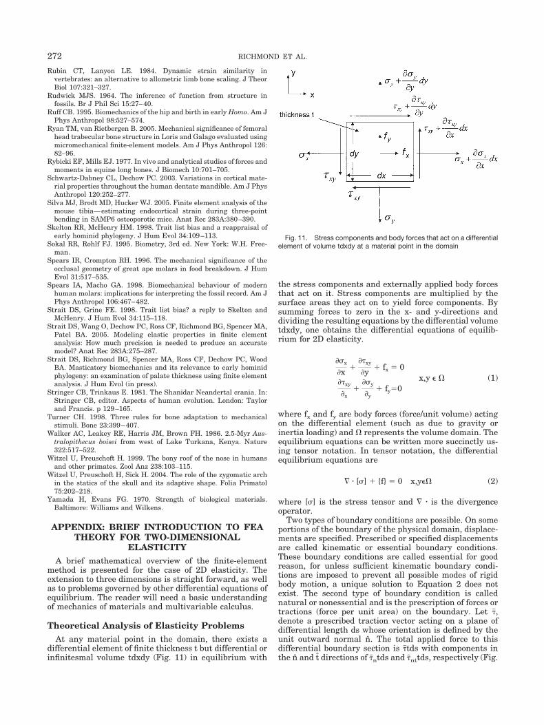
differential element of finite thickness t but differential orinfinitesmal volume tdxdy (Fig. 11) in equilibrium with

the stress components and externally applied body forcesthat act on it. Stress components are multiplied by thesurface areas they act on to yield force components. Bysumming forces to zero in the x- and y-directions anddividing the resulting equations by the differential volumetdxdy, one obtains the differential equations of equilib-rium for 2D elasticity.

��x

�x �xy

�y fx � 0

�xy

�x

��y

�y fy�0

x,y � � (1)

where fx and fy are body forces (force/unit volume) actingon the differential element (such as due to gravity orinertia loading) and � represents the volume domain. Theequilibrium equations can be written more succinctly us-ing tensor notation. In tensor notation, the differentialequilibrium equations are

� � [�] {f} � 0 x,y�� (2)

where [�] is the stress tensor and � � is the divergenceoperator.

Two types of boundary conditions are possible. On someportions of the boundary of the physical domain, displace-ments are specified. Prescribed or specified displacementsare called kinematic or essential boundary conditions.These boundary conditions are called essential for goodreason, for unless sufficient kinematic boundary condi-tions are imposed to prevent all possible modes of rigidbody motion, a unique solution to Equation 2 does notexist. The second type of boundary condition is callednatural or nonessential and is the prescription of forces ortractions (force per unit area) on the boundary. Let �,denote a prescribed traction vector acting on a plane ofdifferential length ds whose orientation is defined by theunit outward normal n. The total applied force to thisdifferential boundary section is �tds with components inthe n and t directions of �ntds and �nttds, respectively (Fig.

Fig. 11. Stress components and body forces that act on a differentialelement of volume tdxdy at a material point in the domain

272 RICHMOND ET AL.

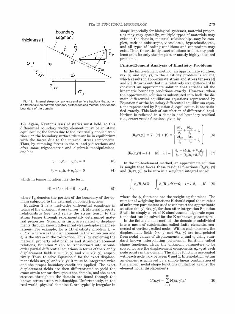
12). Again, Newton’s laws of statics must hold, so thisdifferential boundary wedge element must be in staticequilibrium; the forces due to the externally applied trac-tion � on the boundary surface tds must be in equilibriumwith the forces due to the internal stress components.Thus, by summing forces in the x- and y-directions andafter some trigonometric and algebraic manipulations,one has

�x � �xnx xyny � 0 (3)

�y � xynx �yny � 0 (4)

which in tensor notation has the form

{�} � {n} � [�] � 0 x,y� n (5)

where n denotes the portion of the boundary of the do-main subjected to the externally applied tractions.

Equation 2 is a first-order differential equations interms of the unknown stress tensor [�]. Material propertyrelationships (see text) relate the stress tensor to thestrain tensor through experimentally determined mate-rial properties. Strains, in turn, are related to displace-ments through known differential strain-displacement re-lations. For example, for a 1D elasticity problem εx �du/dx, where u is the displacement in the x-direction andεx is the strain in the x-direction. Thus, by exploiting thematerial property relationships and strain-displacementrelations, Equation 2 can be transformed into second-order partial differential equations in terms of the x and ydisplacement fields u � u(x, y) and v � v(x, y), respec-tively. Thus, to solve Equation 2 for the exact displace-ment fields u(x, y) and v(x, y), it must be integrated twiceand the proper boundary conditions applied. The exactdisplacement fields are then differentiated to yield theexact strain tensor throughout the domain, and the exactstresses throughout the domain are found through theknown stress-strain relationships. Unfortunately, in thereal world, physical domains � are typically irregular in

shape (especially for biological systems), material proper-ties may vary spatially, multiple types of materials mayexist in the domain, material relationships may be com-plex, such as anisotropic, viscoelastic, hyperelastic, etc.,and all types of loading conditions and constraints mayexist. Thus, theoretically exact solutions to elasticity prob-lems exist for only the simplest or mostly highly idealizedproblems.

Finite-Element Analysis of Elasticity ProblemsIn the finite-element method, an approximate solution,

u(x, y) and v(x, y), to the elasticity problem is sought,which results in approximate strain and stress tensors [ε]and [�]. It turns out that it is relatively straightforward toconstruct an approximate solution that satisfies all thekinematic boundary conditions exactly. However, whenthe approximate solution is substituted into both the do-main differential equilibrium equations represented byEquation 2 or the boundary differential equilibrium equa-tions represented by Equation 5, equilibrium is not satis-fied exactly. This lack of satisfaction of differential equi-librium is reflected in a domain and boundary residual(i.e., error) vector functions given by

{R�(x,y)} � � � [�] {f} � ���x

�x

�xy

�y fx

�xy

�x

��y

�y fy

� (6)

{R (x,y)} � {�} � {n} � [�� ] � � �x � (�xnx xyny

�y � (xynx�yny) � (7)

In the finite-element method, an approximate solutionis sought that forces these residual functions {R�(x, y)}and {R (x, y)} to be zero in a weighted integral sense:

� n

�i{R }d� ��

�i{R�}d��0; i�1,2,· · ·,K (8)

where the �i functions are the weighting functions. Thenumber of weighting functions K should equal the numberof unknown parameters used to construct the approximatesolution u(x, y), v(x, y), for then after integration Equation8 will be simply a set of K simultaneous algebraic equa-tions that can be solved for the K unknown parameters.

In the finite-element method, the domain is subdividedinto a mesh of subdomains, called finite elements, con-nected at vertices, called nodes. Within each element, thedisplacement fields u(x, y) and v(x, y) are interpolatedfrom nodal values of displacements ui and vi using stan-dard known interpolating polynomial functions calledshape functions. Thus, the unknown parameters to besolved for are the displacement components ui, vi at eachnode point i in the domain. The shape functions associatedwith each node vary between 0 and 1. Interpolation withinan element is achieved by a simple linear combination ofthe element nodal shape functions multiplied against theelement nodal displacements:

u� e(x,y) � �i � 1

Me

Nie(x, y)�i

e (9)

Fig. 12. Internal stress components and surface tractions that act ona differential element with boundary surface tds at a material point on theboundary of the domain.

273FEA IN FUNCTIONAL MORPHOLOGY

ve(x,y) � �i � 1

Me

Nie(x,y)vi

e (10)

where Me is the number of nodes that define element e andNi

e(x, y) is the shape function associated with node i ofelement e.

Now we return to Equation 8. In the finite-elementmethod, the weighting functions �i are taken to be theshape functions Ni used to interpolate the displacementfields u(x, y) and v(x, y). Here, Ni is the shape functionassociated with node i for each displacement componentand is the result of a simple piecewise combination of allthe element nodal shape functions, Ni

e, that are connectedto node i. Therefore, for 2D elasticity with two displace-ment components, K � 2N, where N equals the totalnumber of nodes. Further, since the domain is subdividedinto finite elements, the boundary and domain integra-tions shown in Equation 8 can be subdivided into a set ofindividual element boundary and domain integrations,making the integrations much easier to compute. Thisalso enables each individual finite element to be unique interms of its material properties and behavior, strain-dis-placement relationships, body forces, loading conditions,etc. Since finite elements can be as small as necessary tocapture the complexity of the problem, the net result isthat no matter how complicated the physical domain is inshape, in known material property relationships and be-havior, in known loading conditions, and in kinematicconstraints, an approximate solution can be obtained viathe finite-element method. In general, the limitations thatmight preclude an acceptably accurate solution from beingobtained are lack of knowledge regarding material prop-erties and associated material behavioral laws, uncer-tainty about kinematic constraints and loading conditions,difficulty in defining necessary geometry, and limitationsin computer resources. The method is also based on theconcept of continuums and therefore is not applicable at

the atomic level where quantum mechanic effects domi-nate.

It is important that any approximate solution be capa-ble of converging toward the theoretically exact solution tothe governing differential equations and imposed bound-ary conditions, if such a solution were known. This meansthat if a sequence of numerical analysis is carried out,with each subsequent analysis having more degrees offreedom (typically realized by refining the mesh withsmaller and smaller elements), the method should con-verge to the theoretically exact solution of the problembeing modeled. For properly constructed meshes, this isindeed the case, for Equation 8 forces the residual func-tions {R�(x, y)} and {R (x, y)} to be mathematically orthog-onal to the weighting functions �i. With mesh refinement,N, the number of weighting functions, �i, increases. Al-though the weighting functions may be relatively simplepolynomials (i.e., linear polynomials if using linear finiteelements), as a set they can approximate more compli-cated functions arbitrarily close. Essentially, this forcesthe residual functions to be mathematically orthogonal toan increasingly more complicated set of functions. In thelimit as N 3 �, the residual functions are forced to beorthogonal to all possible well-behaved functions. Thiscondition only occurs when {R�(x, y)} � 0 and {R (x, y)} �0. Therefore, an exact solution to the governing problemhas been obtained.

Of course, the above discussion addresses only the in-herent discretization error in the finite-element method:the representation of the infinite degrees of freedom of thecontinuum by a finite number of degrees of freedom.Equally and often more important are various modelingerrors introduced into the problem. Idealizations of geom-etry, material property behavior and variability, loadingconditions, constraints, etc., all introduce to some extentmodeling errors that may or may not significantly affectthe analysis result. The analyst must rely on his or herdomain expertise and whenever possible employ experi-mental data to validate finite-element models.

274 RICHMOND ET AL.