Embed Size (px)
Citation preview

Unit root
Financial Time Series Analysis: Part II
Seppo Pynnonen
Department of Mathematics and Statistics, University of Vaasa, Finland
Spring 2017
Seppo Pynnonen Financial Time Series Analysis: Part II

Unit root
1 Unit root
Deterministic trend
Stochastic trend
Testing for unit root
ADF-test (Augmented Dickey-Fuller test)
Testing for more than one unit root
Segmented trends, structural breaks, and smooth transition
Instant occurring: Additive outlier (AO)
Smooth transition
Seppo Pynnonen Financial Time Series Analysis: Part II

Unit root
Deterministic trend1 Unit root
Deterministic trend
Stochastic trend
Testing for unit root
ADF-test (Augmented Dickey-Fuller test)
Testing for more than one unit root
Segmented trends, structural breaks, and smooth transition
Instant occurring: Additive outlier (AO)
Smooth transition
Seppo Pynnonen Financial Time Series Analysis: Part II

Unit root
Deterministic trend
Time series yt
Deterministic trend:
yt = g(t) + ut , (1)
t = 1, . . . ,T and ut is a (zero mean) stationary component(ARMA).
g(t) is the trend component, which typically is some sort ofpolynomial:
g(t) = b0 + b1t + b2t2 + · · ·
Linear trend: g(t) = b0 + bt.
Seppo Pynnonen Financial Time Series Analysis: Part II

Unit root
Deterministic trend
Economic interpretation: Trend aggregates the unobservedvariables affecting yt (growth due to technological innovations,productivity, population growth, etc.) Trending series is notstationary because E[yt ] = g(t).
Stationarity is achieved by detrending: I.e.,
yt = yt − g(t) = ut
is stationary.
Seppo Pynnonen Financial Time Series Analysis: Part II

Unit root
Deterministic trend
Example 1 (Deterministic trend)
Realization from a process
yt = 2 + 0.1t + 3 log t + ut
t = 1, . . . , 100, where ut ∼ NID(0, σ2) with σ = 2.
Seppo Pynnonen Financial Time Series Analysis: Part II

Unit root
Deterministic trend
0 20 40 60 80 100
05
1525
yt = 2 + 0.1t + 3log(t) + ut, where ut ~ NID(0, σ2) with σ = 2y t
0 20 40 60 80 100
05
1525
Trend: g(t) = 2 + 0.1t + 3log(t)
g(t)
0 20 40 60 80 100
−40
24
Random component: ut ~ NID(0, σ2), where σ = 2
Time (t)
u
Seppo Pynnonen Financial Time Series Analysis: Part II

Unit root
Stochastic trend1 Unit root
Deterministic trend
Stochastic trend
Testing for unit root
ADF-test (Augmented Dickey-Fuller test)
Testing for more than one unit root
Segmented trends, structural breaks, and smooth transition
Instant occurring: Additive outlier (AO)
Smooth transition
Seppo Pynnonen Financial Time Series Analysis: Part II
Unit root
Stochastic trend
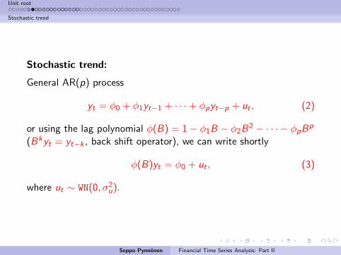
Stochastic trend:
General AR(p) process
yt = φ0 + φ1yt−1 + · · ·+ φpyt−p + ut , (2)
or using the lag polynomial φ(B) = 1− φ1B − φ2B2 − · · · − φpBp
(Bkyt = yt−k , back shift operator), we can write shortly
φ(B)yt = φ0 + ut , (3)
where ut ∼ WN(0, σ2u).
Seppo Pynnonen Financial Time Series Analysis: Part II

Unit root
Stochastic trend
Consider the the special case of a simple AR(1) model
yt = δ + φyt−1 + ut , (4)
where ut ∼ WN(0, σ2u).
The stationarity condition is |φ| < 1.
Seppo Pynnonen Financial Time Series Analysis: Part II

Unit root
Stochastic trend
Alternatively, we can write (4)
yt = δ
t−1∑i=0
φi +t−1∑i=0
φiut−i , (5)
where we have assumed that y0 = 0.
Because |φ| < 1, φi → 0 as i →∞, which implies that the impactof ut−i dies out at exponential rate and the innovation ut has onlya temporary effect on yt
Seppo Pynnonen Financial Time Series Analysis: Part II

Unit root
Stochastic trend
Consider the special case φ = 1, such that
yt = δ + yt−1 + ut , (6)
which is called a random walk (RW) with drift.
Then the representation in (5) becomes
yt = δt + Ut (7)
where
Ut =t−1∑i=0
ut−i = ut + ut−1 + · · ·+ u1, (8)
i.e., the sum of the white noise terms.
Thus, unlike above, the innovations do not die out and ut has apermanent effect on yt .
Seppo Pynnonen Financial Time Series Analysis: Part II

Unit root
Stochastic trend
We observe:E[yt ] = δt (9)
andvar[yt ] = tσ2u (10)
which imply that yt is non-stationary.
The random walk process in equation (6) (with or without a drift)is a model of stochastic trend.
Seppo Pynnonen Financial Time Series Analysis: Part II

Unit root
Stochastic trend
Example 2 (Stochastic trend with drift)
Let δ = .1 in (6), such that
yt = 0.1 + yt + ut .
Below are few realizations from this process.
Seppo Pynnonen Financial Time Series Analysis: Part II

Unit root
Stochastic trend
0 20 40 60 80 100
−20
24
68
yt = δ + yt−1 + ut, where ut ~ NID(0, σ2) with δ = 0.05 and σ = 0.2y t
Seppo Pynnonen Financial Time Series Analysis: Part II

Unit root
Stochastic trend
Example 3 (Coin tossing)
Consider a coin tossing game in which head (H) gains 1 euro and tail (T)loses 1 euro. Let the initial capital be 100 and let St , t = 0, 1, . . . denotethe amount after t tosses, S0 = 100. The St process is
St = St−1 + ut , (11)
t = 1, 2, . . ., where S0 = 100 and ut = 1 or −1, both with probability1/2.The graph below shows few possible realizations of the process in 100tosses.
Seppo Pynnonen Financial Time Series Analysis: Part II

Unit root
Stochastic trend
0 20 40 60 80 100
8090
100
110
120
St = St−1 + ut with S0 = 100
Tosses
S t
Seppo Pynnonen Financial Time Series Analysis: Part II
Unit root
Stochastic trend
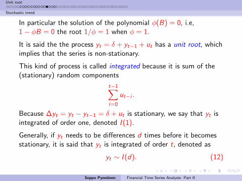
In particular the solution of the polynomial φ(B) = 0, i.e,1− φB = 0 the root 1/φ = 1 when φ = 1.
It is said the the process yt = δ + yt−1 + ut has a unit root, whichimplies that the series is non-stationary.
This kind of process is called integrated because it is sum of the(stationary) random components
t−1∑i=0
ut−i .
Because ∆yt = yt − yt−1 = δ + ut is stationary, we say that yt isintegrated of order one, denoted I (1).
Generally, if yt needs to be differences d times before it becomesstationary, it is said that yt is integrated of order t, denoted as
yt ∼ I (d). (12)
Seppo Pynnonen Financial Time Series Analysis: Part II

Unit root
Stochastic trend
A stationary series is denoted as yt ∼ I (0).
Because for yt ∼ I (d), ∆dyt ∼ I (0), yt is called differencestationary.
In summary, if yt ∼ I (0) :
(i) E[yt ] = µ, for all t.
(ii) An innovation ut has a temporary effect on yt .
(iii) var[yt ] = σ2y <∞ for all t.
(iv) corr[yt , yt+k ] = ρk for all t and ρk decays (exponentially) as kincreases.
Seppo Pynnonen Financial Time Series Analysis: Part II
Unit root
Stochastic trend
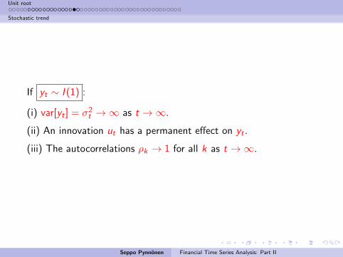
If yt ∼ I (1) :
(i) var[yt ] = σ2t →∞ as t →∞.
(ii) An innovation ut has a permanent effect on yt .
(iii) The autocorrelations ρk → 1 for all k as t →∞.
Seppo Pynnonen Financial Time Series Analysis: Part II

Unit root
Stochastic trend
The ’rule’ in the Box-Jenkins approach: Difference until the seriesbecomes stationary.
Consequence of over differencing: . . .
Checking for unit roots:
(a) Autocorelation function; see ARIMA
(b) Statistical testing
Seppo Pynnonen Financial Time Series Analysis: Part II

Unit root
Testing for unit root1 Unit root
Deterministic trend
Stochastic trend
Testing for unit root
ADF-test (Augmented Dickey-Fuller test)
Testing for more than one unit root
Segmented trends, structural breaks, and smooth transition
Instant occurring: Additive outlier (AO)
Smooth transition
Seppo Pynnonen Financial Time Series Analysis: Part II

Unit root
Testing for unit root
Consideryt = δ + θt + φyt−1 + ut , (13)
where ut ∼ I (0).
Equation (13) is equivalent to [(Augmented) Dickey-Fullerregression]
∆yt = δ + θt + γyt−1 + ut , (14)
in which γ = φ− 1.
Series yt is stationary if |φ| < 1.
If φ = 1 (or γ = 0) then yt ∼ I (1).
In this approach the statistical null hypothesis is: yt ∼ I (1), whichin terms of (14) is
H0 : γ = 0 (15)
with the alternative hypothesis that yt ∼ I (0), or
H1 : γ < 0. (16)
Seppo Pynnonen Financial Time Series Analysis: Part II

Unit root
Testing for unit root
Given the OLS estimators, the test statistic is the t-ratio
t =γ
sγ, (17)
where sγ is the standard error of γ.
The null distribution of t in (17) is not the t-distribution!
Seppo Pynnonen Financial Time Series Analysis: Part II

Unit root
Testing for unit root
Depending on the specification of the ADF regression in (14) thetest static has different distributions.
No intercept (drift) no trend, i.e., in (14) δ = θ = 0, such that
∆yt = γyt−1 + ut . (18)
Drift, no trend, or δ 6= 0 and θ = 0 in (14), such that
∆yt = δ + γyt−1 + ut (19)
The model in (17) is the general one allowing both drift and trend.
Note that under the null hypothesis drift (δ)implies linear trendand the trend (θt) in (14) implies quadratic trend.
Seppo Pynnonen Financial Time Series Analysis: Part II

Unit root
Testing for unit root
The finite sample distribution of t is unknown, but its asymptoticdistribution is known (under certain assumptions).
Example 4
Unit root in DAX index.
Weekly data 1990-2011 (Jan)
EViews results are given below, R (with urca package) example detailedin the class-room.- log indexautocorrelationsvarious unit root tests available in EWiews and in R.
Seppo Pynnonen Financial Time Series Analysis: Part II
Unit root
Testing for unit root
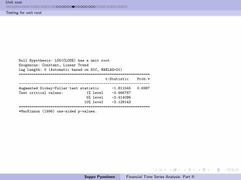
Null Hypothesis: LOG(CLOSE) has a unit root
Exogenous: Constant, Linear Trend
Lag Length: 0 (Automatic based on SIC, MAXLAG=21)
==============================================================
t-Statistic Prob.*
--------------------------------------------------------------
Augmented Dickey-Fuller test statistic -1.811545 0.6987
Test critical values: 1% level -3.966787
5% level -3.414086
10% level -3.129143
==============================================================
*MacKinnon (1996) one-sided p-values.
Seppo Pynnonen Financial Time Series Analysis: Part II

Unit root
Testing for unit root
Augmented Dickey-Fuller Test Equation
Dependent Variable: D(LOG(CLOSE))
Method: Least Squares
Sample (adjusted): 12/03/1990 1/31/2011
Included observations: 1053 after adjustments
==============================================================
Variable Coefficient Std. Err t-Stat Prob.
--------------------------------------------------------------
LOG(CLOSE(-1)) -0.005871 0.003241 -1.811545 0.0703
C 0.046698 0.024490 1.906820 0.0568
@TREND(11/26/1990) 6.13E-06 5.40E-06 1.133601 0.2572
==============================================================
R-squared 0.003415 Mean dependent var 0.001530
Adjusted R-squared 0.001516 S.D. dependent var 0.031398
S.E. of regression 0.031374 Akaike info criterion -4.082832
Sum squared resid 1.033542 Schwarz criterion -4.068703
Log likelihood 2152.611 Hannan-Quinn criter. -4.077475
F-statistic 1.798834 Durbin-Watson stat 2.043702
Prob(F-statistic) 0.166001
==============================================================
Seppo Pynnonen Financial Time Series Analysis: Part II

Unit root
Testing for unit root
The unit root hypothesis is strongly accepted.
Unit root in the first differences?
Null Hypothesis: D(LOG(CLOSE)) has a unit root
Exogenous: Constant
Lag Length: 0 (Automatic based on SIC, MAXLAG=21)
==============================================================
t-Statistic Prob.*
--------------------------------------------------------------
Augmented Dickey-Fuller test statistic -33.27403 0.0000
Test critical values: 1% level -3.436348
5% level -2.864077
10% level -2.568172
==============================================================
*MacKinnon (1996) one-sided p-values.
Unit root hypothesis in the returns (log-differences) is clearly rejected.
Conclusion: log(DAX) ∼ I (1).
Examining the autocorrelation function would lead to the same
conclusion.
Seppo Pynnonen Financial Time Series Analysis: Part II

Unit root
Testing for unit root
Example 5
UK interest rate spread.
1950 1960 1970 1980 1990 2000
-50
510
15
Monthly UK short and long interest rates
Jan 1952 to Dec 2005
Interest
rate
10 y Gilt91 days TBSpread
Short rate Long rate Spread
ADF -2.7628 -1.5901 -3.835
Critical values for test statistics:
1pct 5pct 10pct
-3.43 -2.86 -2.57
Seppo Pynnonen Financial Time Series Analysis: Part II

Unit root
Testing for unit root
Both unit root hypotheses are accepted at the 5% level.
According to the expectations hypothesis (EH) of the term structure ofinterest rates the long rate is the weighted average of the current andexpected rates of the future short rates.
This implies that the spread should be stationary.
Above the unit root hypothesis for spread is rejected, indicating support
for the EH.
Seppo Pynnonen Financial Time Series Analysis: Part II

Unit root
Testing for unit root
Other popular unit root tests: Phillips-Perron (PP) (Biometrika,1988, 335–346), Elliot-Rottenberg-Stock (ERS) (Econometrica,1996, 813–836)
ERS is supposed be more efficient than the others.
Short rate Long rate Spread
ERS -1.853 -0.8955 -2.3904
Critical values of DF-GLS are:
1pct 5pct 10pct
critical values -2.57 -1.94 -1.62
Seppo Pynnonen Financial Time Series Analysis: Part II

Unit root
Testing for unit root1 Unit root
Deterministic trend
Stochastic trend
Testing for unit root
ADF-test (Augmented Dickey-Fuller test)
Testing for more than one unit root
Segmented trends, structural breaks, and smooth transition
Instant occurring: Additive outlier (AO)
Smooth transition
Seppo Pynnonen Financial Time Series Analysis: Part II
Unit root
Testing for unit root
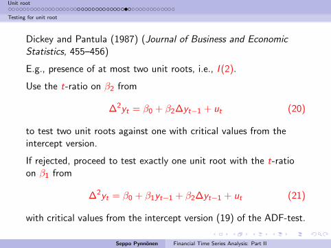
Dickey and Pantula (1987) (Journal of Business and EconomicStatistics, 455–456)
E.g., presence of at most two unit roots, i.e., I (2).
Use the t-ratio on β2 from
∆2yt = β0 + β2∆yt−1 + ut (20)
to test two unit roots against one with critical values from theintercept version.
If rejected, proceed to test exactly one unit root with the t-ratioon β1 from
∆2yt = β0 + β1yt−1 + β2∆yt−1 + ut (21)
with critical values from the intercept version (19) of the ADF-test.
Seppo Pynnonen Financial Time Series Analysis: Part II

Unit root
Testing for unit root
Example 6
UK interest rates I (2)? (Classroom example).
1950 1960 1970 1980 1990 2000
−10
−50
510
1520
Monthly UK short and long interest rates
Month
Rate
(% pa
)
20 year gilt91 day TBSpread
Seppo Pynnonen Financial Time Series Analysis: Part II

Unit root
Segmented trends, structural breaks, and smooth transition1 Unit root
Deterministic trend
Stochastic trend
Testing for unit root
ADF-test (Augmented Dickey-Fuller test)
Testing for more than one unit root
Segmented trends, structural breaks, and smooth transition
Instant occurring: Additive outlier (AO)
Smooth transition
Seppo Pynnonen Financial Time Series Analysis: Part II
Unit root
Segmented trends, structural breaks, and smooth transition1 Unit root
Deterministic trend
Stochastic trend
Testing for unit root
ADF-test (Augmented Dickey-Fuller test)
Testing for more than one unit root
Segmented trends, structural breaks, and smooth transition
Instant occurring: Additive outlier (AO)
Smooth transition
Seppo Pynnonen Financial Time Series Analysis: Part II

Unit root
Segmented trends, structural breaks, and smooth transition
Perron (1989, Econometrica) generalized the unit root testing(that has possibly a drift and a linear trend) to allow for one timechange in the structure at an unknown time TB (break point),1 < TB < T .
TB must be determined prior testing.
Occurring instantly/smoothly?
(a) Shift in the intercept of the trend (crash model)(b) shift in intercept and slope (crash/changing growth)
(c) smooth shift in the slope (joined segments)
Seppo Pynnonen Financial Time Series Analysis: Part II

Unit root
Segmented trends, structural breaks, and smooth transition
Example 7
Certain types of breaks.
0 100 200 300 400 500 600
10.0
11.0
12.0
13.0
No Breaks: Random walk with drift
time
y t
y t = β + yt−1 + ut
yt = y0 + βt + ut
0 100 200 300 400 500 600
10.0
11.0
12.0
13.0
Model (a): 'Crash'
time
y t
y t = β + yt−1 + ut
yt = y0 + βt + ut yt = β + θDTBt + yt−1 + ut
yt = y0 + θDTBt + βt + ut
0 100 200 300 400 500 600
1011
1213
1415
Model (b): 'Crash/changing growth'
time
y t
y t = β + yt−1 + ut
yt = y0 + βt + ut
yt = β + yt−1 + θDTBt + γDUt + ut
yt = y0 + βt + θDUt + γDTt + ut
0 100 200 300 400 500 60010
1112
1314
15
Model (c): 'Smooth slope shift'
time
y ty t = β + yt−1 + ut
yt = µ + βt + ut
yt = µ + βt + γDTt + ut
yt = β + yt−1 + γDUt + ut
Seppo Pynnonen Financial Time Series Analysis: Part II

Unit root
Segmented trends, structural breaks, and smooth transition
Define dummy variables:
DTBt = 1, if t = TB + 1, = 0 otherwise
DUt = 1, if t > TB , = 0 otherwise (22)
DTt = t − TB , if t > TB , = 0 otherwise.
Note that DTBt = ∆DUt = ∆2DRt .
Null hypothesis models of (a)–(c)
yt = β + yt−1 + θDTBt + ut (23)
yt = β + yt−1 + θDTBt + γDUt + ut (24)
yt = β + yt−1 + γDTt + ut (25)
Seppo Pynnonen Financial Time Series Analysis: Part II

Unit root
Segmented trends, structural breaks, and smooth transition
Trend stationary alternative hypotheses of (a)–(c)
yt = µ+ βt + θDTBt + ut (26)
yt = µ+ βt + θDUt + γDTt + ut (27)
yt = µ+ βt + γDTt + ut (28)
The error term ut is assumed stationary.
Seppo Pynnonen Financial Time Series Analysis: Part II

Unit root
Segmented trends, structural breaks, and smooth transition
Model (a): One time change by magnitude θ
Model (b): Null: Changing growth, drift changes from β to β + θγat time TB + 1 and then to β + γ afterwards. Alternative:Intercept changes by θ and slope by γ at TB + 1.
Model (c): Null: Drift changes to β + γ. Alternative: Bothsegments of the trends are equal at TB .
Seppo Pynnonen Financial Time Series Analysis: Part II
Unit root
Segmented trends, structural breaks, and smooth transition
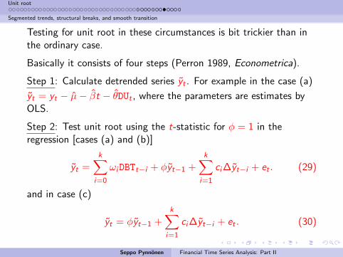
Testing for unit root in these circumstances is bit trickier than inthe ordinary case.
Basically it consists of four steps (Perron 1989, Econometrica).
Step 1: Calculate detrended series yt . For example in the case (a)
yt = yt − µ− βt − θDUt , where the parameters are estimates byOLS.
Step 2: Test unit root using the t-statistic for φ = 1 in theregression [cases (a) and (b)]
yt =k∑
i=0
ωiDBTt−i + φyt−1 +k∑
i=1
ci∆yt−i + et . (29)
and in case (c)
yt = φyt−1 +k∑
i=1
ci∆yt−i + et . (30)
Seppo Pynnonen Financial Time Series Analysis: Part II

Unit root
Segmented trends, structural breaks, and smooth transition
Step 3: Compute the set of t-statistics for all possible breaks andselect the date for the break TB for which the t-statistic isminimized.
Step 4: Compare the selected t-value of Step 3 to appropriatecritical value (Tables given e.g. in Vogelsang and Perron 1998International Economic Review).
Seppo Pynnonen Financial Time Series Analysis: Part II

Unit root
Segmented trends, structural breaks, and smooth transition1 Unit root
Deterministic trend
Stochastic trend
Testing for unit root
ADF-test (Augmented Dickey-Fuller test)
Testing for more than one unit root
Segmented trends, structural breaks, and smooth transition
Instant occurring: Additive outlier (AO)
Smooth transition
Seppo Pynnonen Financial Time Series Analysis: Part II

Unit root
Segmented trends, structural breaks, and smooth transition
Rather than instantaneous break (alternative hypothesis), thetrend can change smoothly. In such a case one possibility to modelit is to utilize logistic smooth transition regression (LSTR):
Alternative hypotheses of (a)–(c)
yt = µ1 + µ2St(γ,m) + ut (31)
yt = µ1 + β1t + µ2St(γ,m) + ut (32)
yt = µ1 + β1t + µ2St(γ,m) + β2tSt(γ,m) + ut , (33)
where
St(γ,m) =1
1 + exp(−γ(t −mT )). (34)
0 ≤ St(γ,m) ≤ 1. Parameter m determines the timing of thetransition midpoint.
Seppo Pynnonen Financial Time Series Analysis: Part II
Unit root
Segmented trends, structural breaks, and smooth transition
For γ > 0, S−∞(γ,m) = 0, S∞(γ,m) = 1, and SmT (γ,m) = 0.5.
γ determines the speed of transmission, for γ = 0, St(0,m) = 0.5.
LSTAR models are estimated by nonlinear least squares (NLS) andunit root is tested by ADF applied to the residuals of the NLSregression (more details in Laybourne, Newbold, and Vougas 1998Journal of Time Series Analysis).
Seppo Pynnonen Financial Time Series Analysis: Part II