Munich Personal RePEc Archive

Financial Innovations and Monetary

Policy in Kenya

Nyamongo, Esman and Ndirangu, Lydia Ndirangu2

Central Bank of Kenya

December 2013

Online at https://mpra.ub.uni-muenchen.de/52387/

MPRA Paper No. 52387, posted 21 Dec 2013 09:10 UTC

FINANCIAL INNOVATIONS AND MONETARY POLICYIN KENYA1

Esman Nyamongo and Lydia Ndirangu2

Draft Paper for Comments

Submitted to the African Economic Research Consortium (AERC) Biannual Research

Workshop on Financial Inclusion and Innovation in Africa, 1-5 December 2013.

1 Disclaimer: The views expressed in this paper are solely those of the authors and do not reflect the views ofthe Central Bank of Kenya.2 Email: NyamongoEM@centralbank.go.ke; lndirangu@ksms.or.ke;

AbstractThe objective of this study is to analyze the effects of financial innovation in the banking sector on the conduct ofmonetary policy in Kenya during 1998-2012. The country has witnessed a number of financial innovations during thisperiod. The study focuses on whether these wave of financial innovations have impacted on the transmission mechanismof monetary policy, and if so how. The results show that the innovations have improved the monetary policyenvironment in Kenya as the proportion of the unbanked population has declined coupled with gradual reduction incurrency outside banks. However, the period post 2007 when the country has experienced the fastest pace of financialinnovation, is associated with instability in the money multiplier, income velocity of money and the money demand.However, recent trends point towards stabilization pointing to the need for further examination establish whetherindeed the break in trend is of structural or transitory in nature. A structural break raises questions on the credibilityof the current monetary targeting framework in use in Kenya, in view of which a more flexible framework should beadopted. Overall, the results show that financial innovation has had positive outcomes and seems to improve the interestrate channel of monetary policy transmission.

1

1.0 INTRODUCTION

The term financial innovation has been used in a variety of content to refer to a wide range ofchanges and developments affecting financial markets. In a narrow sense, the term can be used torefer solely to the introduction of new financial instruments. In a broader sense, it can encapsulatechanges in the structure and depth of financial markets, in the role of financial institutions, themethods by which financial services are provided and the introduction of products and proceduresin the wake of deregulation.

In recent decades, financial sectors of many countries have undergone significant changes againstthe background of general trend towards deregulation, globalization, and development of theinternet and the resulting explosion of e-commerce. Technological innovation and falling costs incomputing and telecommunications, have especially aided growth of the most recent innovations inpayments — electronic payments (e-payments). In the history of money, “…there has been onlyfour times that we have changed the way we pay”3. In the beginning, there was barter, then coinage;coins to paper; paper to cheques; and then cards. Developments in technology andtelecommunication have brought about these changes.

The spread of the financial innovations vary unevenly between countries, partly due to differences infactors such as regulatory frameworks and readiness of telecommunication infrastructure. Forinstance, while payment services based on the internet and mobile phones are prolific in theadvanced economies, in some of the emerging and low-income economies, the pace anddevelopment of e-payments appears slow and uneven.

However, in the recent years, mobile technology has flourished throughout the developing worldfaster than any other technology in history. With this growth comes an equally remarkable surge ofmessaging services, providing not just a means of personal communications, but also a number ofvaluable information services, the most impressive being mobile money. The money transferservices are available to millions of previously underserved people, allowing them to safely sendmoney and pay bills for the first time without having to rely exclusively on cash. The global leader inmobile money is Kenya, where mobile network operator Safaricom launched M-Pesa in March 2007.Six years into its existence, the amount transacted through the mobile networks between January andSeptember 2013 accumulated to 1.37 trillion – a figure that is very close to the national budget ofKShs.1.46 trillion (US$17.5 billion) for 2012/2013 fiscal year, and also a third of Kenya’s GrossDomestic Product (GDP) of KShs.3.7 trillion (US$41.8 billion). The rise in the cashless transactionvalue is attributed to increasing partnerships between banks and mobile service providers. Theincreased transactions have made Kenya stamp its authority as the leading mobile money market inthe world, with very few countries recording success close to Kenya’s. This growth in mobile moneyusage has been credited with a doubling of access to formal financial services from 32 percent in

3 Observes David Evans, co-author of “Paying with Plastic: The Digital Revolution in Buying and Borrowing”, D. Evans and R.Schmalensee, MIT Press, 2004.

2

2006 to 67 percent in 2013 and a decline of those using informal financial services to only 8% fromabout 33 percent over the same period (FinAccess, 2013).

The country has also experienced an expansion in use of debit cards and Automated TellerMachines (ATMs). In addition, at the institutional level, the Central Bank of Kenya (CBK) hasfostered changes in the legal and regulatory framework to promote financial inclusion and e-payment systems as the basis for financial transactions and settlements. The enactment of theNational Payment Systems Act of 2011 and the issuance of guidelines for the provision of electronicretail transfers and e-money in 2012; the issuance of the agency banking guidelines in 2010 andlicensing of deposit taking micro-finance institutions are a reflection of these efforts.

While financial innovations can help to increase the efficiency of the financial system, whichfacilitates the operation of monetary policy, it can at the same time complicate the environment inwhich monetary policy operates (Angeloni, et al, 2003; Noyer, 2008). The experience of the 2007/8financial turmoil demonstrates that financial innovation is not a smooth process. The challengesconfronting central banks, therefore, are not only directed at the attainment of efficiency, but alsothe attainment of stability in the financial system. Some financial innovation may affect the way inwhich the economy reacts to monetary policy, or may affect the information content of theindicators that central banks regularly monitor and that serve as a basis for taking policy decisions.Noyer (2007) observes that “it is clearly not a surprise, at a time of burgeoning financial innovationto observe signs of instability in money demand. New products and new intermediaries tend to blurthe distinction between monetary and non-monetary assets and to modify the financial behaviour ofeconomic agents”. It’s is such effects that this paper explores for Kenya and how they may haveimpacted on the transmission of monetary policy.

The rest of the paper is organized as follows. Section 2 provides a brief account of recentdevelopments in the banking sector in Kenya and a review of some relevant studies. Section 3outlines the methodology and data used. Section 4 reports the empirical results, while Section 5offers concluding remarks and draws policy implications.

3

2.0 REVIEW OF BANKING SECTOR DEVELOPMENT AND FINANCIALINNOVATIONS IN KENYA

Financial innovation which has been witnessed in Kenya has come with benefits. As shown onFigure 1, the country’s banking sector has been developing. While the ratio of deposits to GDP roseby only 6 percentage points between 1996 and 2007 (from 27 percent to 33 percent), it increased by11 percentage points between 2007 and 2012, to stand at 44 percent. The ratio of M2/GDP whichstood at 34 percent in 2007 increased to approximately 42 percent in 2013.

Figure 1: Banking sector developments in Kenya

Source: Central Bank of Kenya

25.0

30.0

35.0

40.0

45.0

50.0

% o

f G

DP

Deposits to GDP

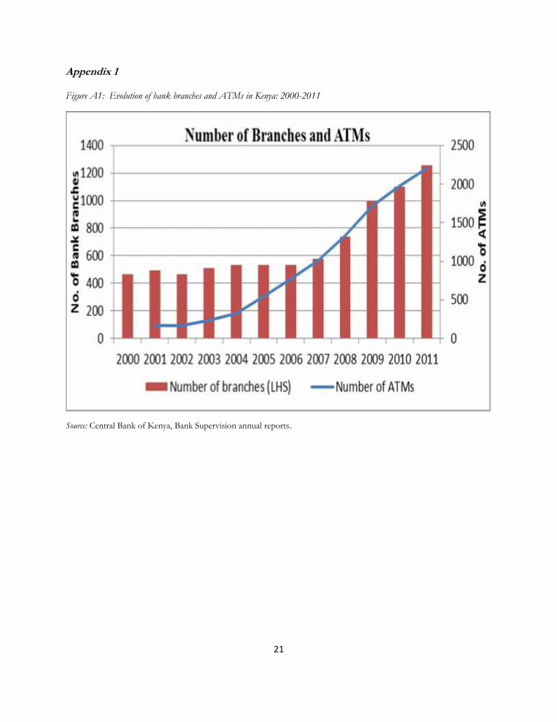
Associated with this rapid expansion in the banking sector is a range of financial innovations: theATMs and debit cards introduced in the late 1990s; the electronic money introduced in early 2007;the agent banking model introduced in mid-2010; and the allowing of deposit taking micro financeinstitutions (MFI). The number of bank branches in Kenya increased from 465 in 2000 to 1279 in2012 with the largest increase being recorded after 2007 (Figure A1 in the appendix). A similar trendis observed for ATMs. The number of ATMs increased from a low of 168 machines in 2001 to 540in 2006 and then to 2381 in 2012. The fast growth period (2007-2012) also corresponds to theexpansion of the mobile money transfer services across the country.

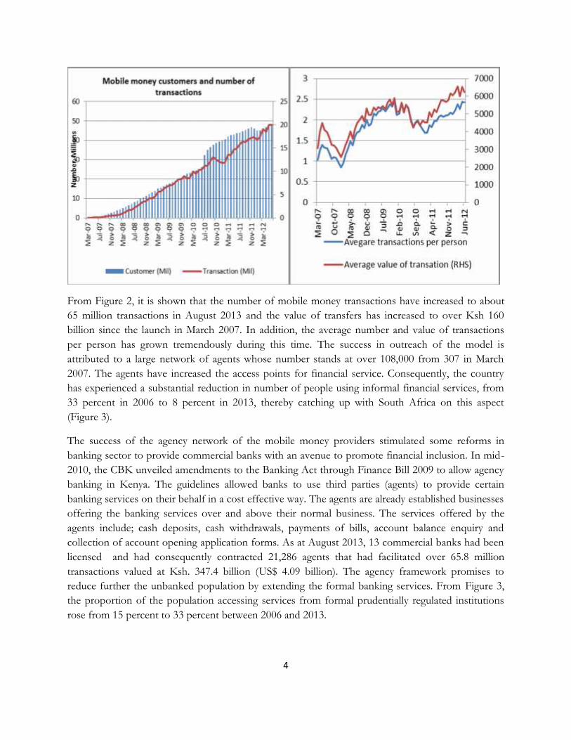
Figure 2: Evolution of Mobile Money in Kenya: May 2007-Aug 20134

4 The transaction data is aggregated for all the mobile money services providers. Currently there are 4 mobile telephoneoperators in Kenya, namely safaricom, Airtel, Orange and YU.

4

From Figure 2, it is shown that the number of mobile money transactions have increased to about

65 million transactions in August 2013 and the value of transfers has increased to over Ksh 160

billion since the launch in March 2007. In addition, the average number and value of transactions

per person has grown tremendously during this time. The success in outreach of the model is

attributed to a large network of agents whose number stands at over 108,000 from 307 in March

2007. The agents have increased the access points for financial service. Consequently, the country

has experienced a substantial reduction in number of people using informal financial services, from

33 percent in 2006 to 8 percent in 2013, thereby catching up with South Africa on this aspect

(Figure 3).

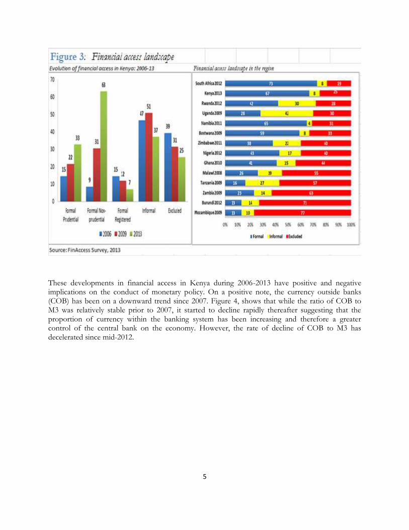
The success of the agency network of the mobile money providers stimulated some reforms in

banking sector to provide commercial banks with an avenue to promote financial inclusion. In mid-

2010, the CBK unveiled amendments to the Banking Act through Finance Bill 2009 to allow agency

banking in Kenya. The guidelines allowed banks to use third parties (agents) to provide certain

banking services on their behalf in a cost effective way. The agents are already established businesses

offering the banking services over and above their normal business. The services offered by the

agents include; cash deposits, cash withdrawals, payments of bills, account balance enquiry and

collection of account opening application forms. As at August 2013, 13 commercial banks had been

licensed and had consequently contracted 21,286 agents that had facilitated over 65.8 million

transactions valued at Ksh. 347.4 billion (US$ 4.09 billion). The agency framework promises to

reduce further the unbanked population by extending the formal banking services. From Figure 3,

the proportion of the population accessing services from formal prudentially regulated institutions

rose from 15 percent to 33 percent between 2006 and 2013.

5

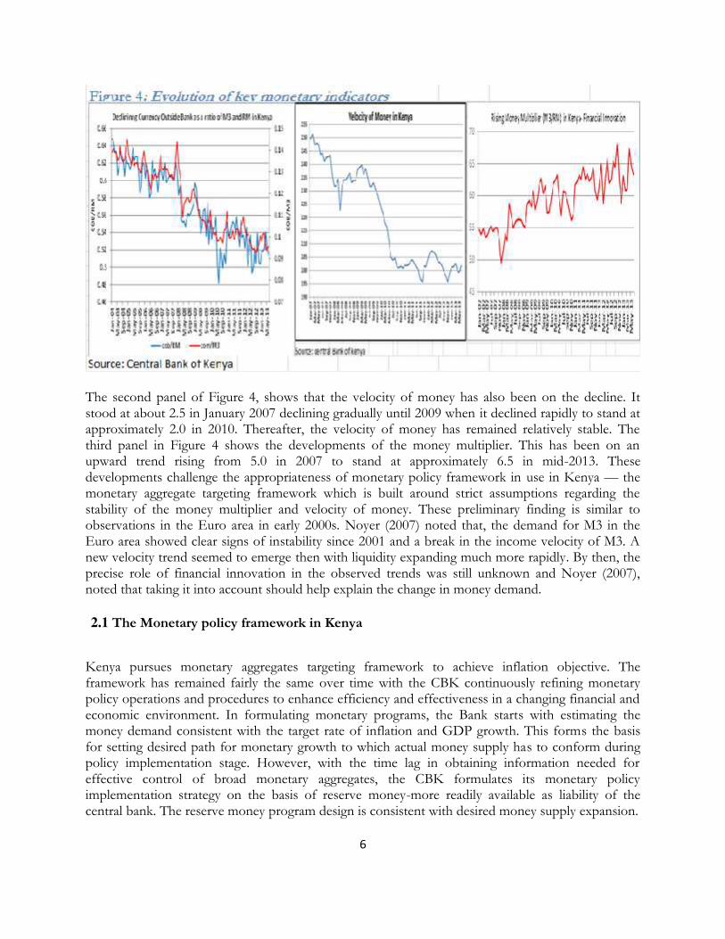
These developments in financial access in Kenya during 2006-2013 have positive and negativeimplications on the conduct of monetary policy. On a positive note, the currency outside banks(COB) has been on a downward trend since 2007. Figure 4, shows that while the ratio of COB toM3 was relatively stable prior to 2007, it started to decline rapidly thereafter suggesting that theproportion of currency within the banking system has been increasing and therefore a greatercontrol of the central bank on the economy. However, the rate of decline of COB to M3 hasdecelerated since mid-2012.

6

The second panel of Figure 4, shows that the velocity of money has also been on the decline. Itstood at about 2.5 in January 2007 declining gradually until 2009 when it declined rapidly to stand atapproximately 2.0 in 2010. Thereafter, the velocity of money has remained relatively stable. Thethird panel in Figure 4 shows the developments of the money multiplier. This has been on anupward trend rising from 5.0 in 2007 to stand at approximately 6.5 in mid-2013. Thesedevelopments challenge the appropriateness of monetary policy framework in use in Kenya — themonetary aggregate targeting framework which is built around strict assumptions regarding thestability of the money multiplier and velocity of money. These preliminary finding is similar toobservations in the Euro area in early 2000s. Noyer (2007) noted that, the demand for M3 in theEuro area showed clear signs of instability since 2001 and a break in the income velocity of M3. Anew velocity trend seemed to emerge then with liquidity expanding much more rapidly. By then, theprecise role of financial innovation in the observed trends was still unknown and Noyer (2007),noted that taking it into account should help explain the change in money demand.

2.1 The Monetary policy framework in Kenya

Kenya pursues monetary aggregates targeting framework to achieve inflation objective. Theframework has remained fairly the same over time with the CBK continuously refining monetarypolicy operations and procedures to enhance efficiency and effectiveness in a changing financial andeconomic environment. In formulating monetary programs, the Bank starts with estimating themoney demand consistent with the target rate of inflation and GDP growth. This forms the basisfor setting desired path for monetary growth to which actual money supply has to conform duringpolicy implementation stage. However, with the time lag in obtaining information needed foreffective control of broad monetary aggregates, the CBK formulates its monetary policyimplementation strategy on the basis of reserve money-more readily available as liability of thecentral bank. The reserve money program design is consistent with desired money supply expansion.

7

Central banks cannot determine directly the rate of monetary expansion. The rate of monetaryexpansion depends on a multitude of factors outside the immediate sphere of influence of a centralbank. This occasions the monetary authorities to identify yet another intermediate target: the interestrate or monetary base. Once the link between the monetary base and the money supply isunderstood, a strong positive correlation between the evolution of the money supply and that ofprices is postulated. This correlation is not always straightforward, because it depends on thestability and predictability of velocity, and, ultimately, on money demand.

In 2007, the Central Bank of Kenya Act was amended to allow the formation of the Monetary PolicyCommittee (MPC). The Committee is charged with the responsibility for formulating monetarypolicy. The MPC meets every sixty days, unless the macroeconomic environment necessitates morefrequent meetings. The Committee meets to review the macroeconomic environment on the basisof which a decision is made on the monetary policy stance. This is done, mainly, by setting thecentral bank rate which is expected to signal and coordinate other rates in the market with a view tostabilizing the economy.

The monetary aggregate framework is conducted via financial programming with the broad money(M3) as the intermediate target while reserve money serves as the operating target. The key tools thatthe CBK uses to implement the programme are:

• Open Market Operations (OMO) — the bank relies heavily on this instrument.

• Reserve Requirements—currently 4.5 percent.

• Other Instruments—these include rediscount facilities and lender of last resort facility,which are not very popular.

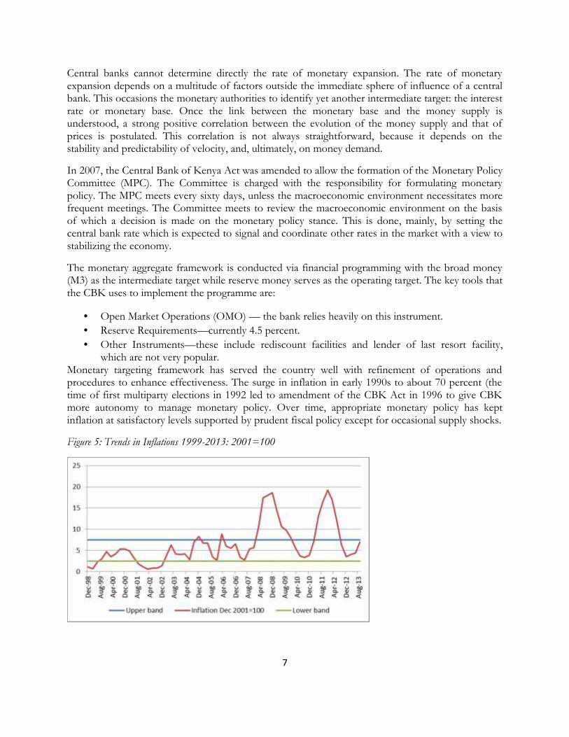
Monetary targeting framework has served the country well with refinement of operations andprocedures to enhance effectiveness. The surge in inflation in early 1990s to about 70 percent (thetime of first multiparty elections in 1992 led to amendment of the CBK Act in 1996 to give CBKmore autonomy to manage monetary policy. Over time, appropriate monetary policy has keptinflation at satisfactory levels supported by prudent fiscal policy except for occasional supply shocks.

Figure 5: Trends in Inflations 1999-2013: 2001=100

8

2.2 Literature Review

The literature on financial innovation is still evolving as new financial instruments; financial servicesand operational techniques continue to enter the market. The existing scanty literature has focusedon evolution of the financial system in the developed world with few studies focusing on developingcountries. Existing studies have analyzed the linkages between general financial innovation andmonetary policy, growth and inflation and some analysis of linkages between specific financialinnovation products, macroeconomic variables and monetary policy transmission mechanisms. Thissection briefly presents a survey of some theoretical and empirical work with a bias towardsdeveloping economies.

The first strand of literature analyses the impact of electronic money on the central bank’s ability tocontrol money supply. This literature is controversial on this aspect, with one line of thought arguingthat increasing usage of electronic money would make it difficult for central banks to supervise andmeasure monetary base (see Kobrin 1997, Friedman, 1999). The other strand holds a more optimisticview and note that the fears for the future of monetary policy may be overstated (see Bert, 1996;

Helleiner, 1998; Freedman, 2000; Goodhart, 2000; and Woodford, 2000). Notably, Helleiner (1998),observes that “new forms of electronic money are unlikely to pose a significant threat to the powerof the sovereign state". Woodford (2000) adds that even if there may be vast changes in e-money,one day, these changes are unlikely to interfere with the conduct of monetary policy. Which view isright?

The main goal of monetary policy is to keep the level of aggregate expenditure in an economybroadly consistent with production capacity; in other words, to guide the ship of state between thedangers of rampant inflation and that of prolonged recession. If electronic money can be expectedto have any impact at all on the effectiveness of policy, it will be through its influence on thelinkages between central-bank decisions and market spending.

Extensive literature explores the effect of financial innovation on the stability of the money demandfunction, with a general consensus that evolution of new financial products creates instability in thetraditional money demand function. Arrau and De Gregorio (1993) examined the money demandequations in Chile and Mexico. Their results suggested that there is an important permanentcomponent in the demand for money not captured by traditional variables but by financialinnovation, which is modeled as an unobservable shock that has permanent effects on moneydemand. Using market share of credit cards as an indicator of financial innovation, Viren (1992)empirically examined the relationship between financial innovations and currency demand. Theresults showed that credit card transactions have a strong offsetting effect on currency demand.

A similar study by Al-Sowaidi and Darrat (2006) examined the effects of financial innovations inBahrain, the UAE and Qatar on the long-run money demand. The study found no undue shifts inthe equilibrium money demand relationship despite the fast pace of financial innovation experiencedin the three countries. The findings were robust to the measure of the money stock —narrow orbroad.

In Korea, Cho and Miles (2007) found a downward trend in velocity which was attributed tomonetization of the economy. It is expected that velocity should increase over time as payments

9

systems evolve or cash management improves. Although financial liberalization may allow agents tominimize cash balances, it also permits greater interest to be paid on many categories of money. Thebasic argument in the perverse sign observed in the Korean case is based on the fact that, there isincreased willingness to hold M2 as income increases. The coefficient of real GDP was more thanunity indicating a high level of monetization in the Korean economy.

A few studies exist focusing on the examination of the linkages between financial innovation and thestability of the money demand function in Africa. Using Granger causality and VAR methodologies,Kovanen (2004) examined the determinants of currency demand and inflation dynamics inZimbabwe. The author measured financial innovation as the ratio of broad money to currency.However, the results from the VAR estimation for financial innovation are not significant. Lungu etal (2012) did a similar study using Malawian data but in this case financial innovation has asignificant effect on the demand for money in the short run.

Sichei and Kamau (2012) conducted a similar study using Kenyan Data. They used the number ofATMs as a proxy for financial innovation. Their results did not indicate any significant effect ofinnovations on the demand for money. However, this study used only one measure of financialinnovation, which is also not widespread across the country. While acknowledging that the data forother more inclusive measures such as M-Pesa may not have been available and adequate in terms ofobservations to allow plausible empirical investigation, the authors did not explore other financialinnovation measures used in previous studies. They, however, demonstrated the instability of moneydemand post 2007. Weil et al., 2012 also showed this instability.

Studies conducted on Kenya in the 1980s and 1990s (see Dharat 1985; Mwega, 1990; Adam, 1990)shows that money demand was stable at the time. Of particular interest is a study by Dharat (1985),where special attention was paid to the model specification, its dynamic structure and to its temporalstability. Following this approach the study showed that for both conventional definitions of money(the narrow and broad), the theoretical model fits the Kenyan data quite well, and the variables wereall statistically significant and with the anticipated signs. Based on a battery of tests, the resultssuggested that the estimated money demand equation for Kenya was temporally stable. Turning tothe open-economy nature of the money demand model, it was found that the foreign interest rateplays a significant role in the Kenyan money demand equations.

3.0 METHODOLOGY

To investigate the effect of financial innovation on the conduct of monetary policy the obviousstarting point is to provide analysis on whether these innovations have led to a breakdown of thevarious assumptions underlying the monetary aggregates framework in Kenya. The monetaryaggregates framework works on the assumption that the money demand is stable. In addition, itassumes that the velocity of circulation and the money multiplier are stable. Therefore to test theeffect of financial innovation on the conduct of monetary policy we: (i) test for stability of incomevelocity of money, money multiplier and the money demand (ii) investigate whether or not theinnovations have impacted the monetary policy transmission.

10

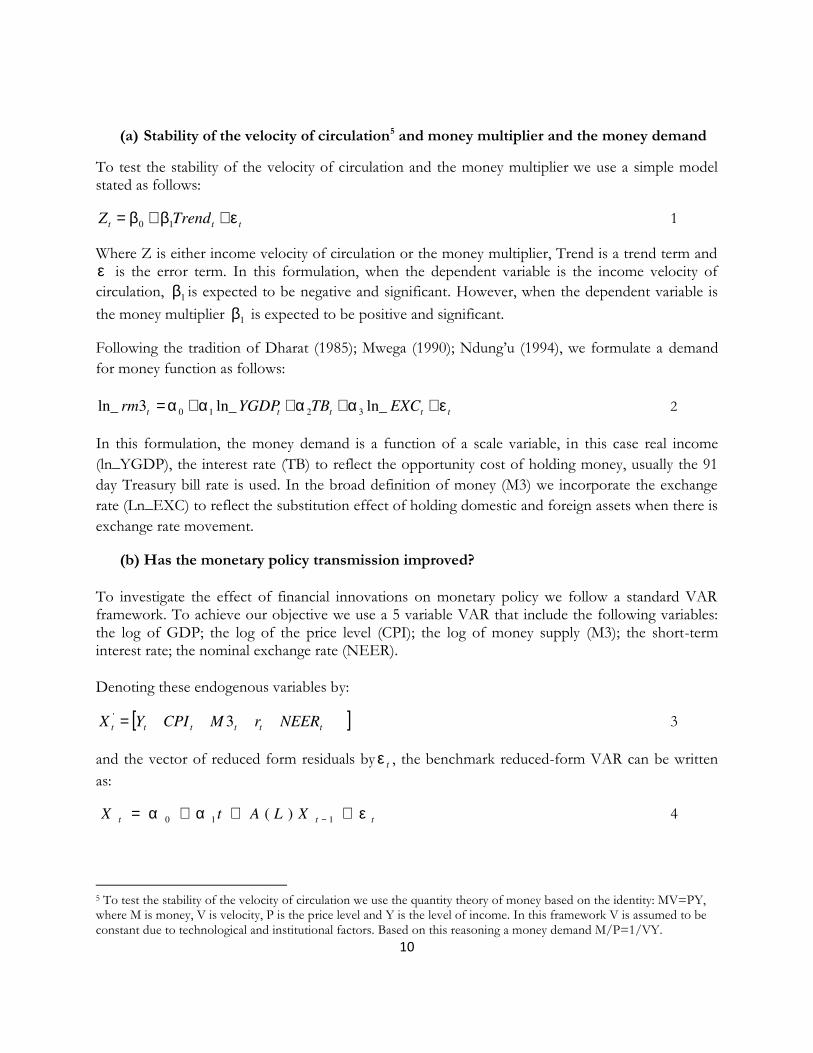
(a) Stability of the velocity of circulation5 and money multiplier and the money demand

To test the stability of the velocity of circulation and the money multiplier we use a simple modelstated as follows:

tttTrendZ εββ ++= 10 1

Where Z is either income velocity of circulation or the money multiplier, Trend is a trend term andε is the error term. In this formulation, when the dependent variable is the income velocity of

circulation, 1β is expected to be negative and significant. However, when the dependent variable is

the money multiplier1β is expected to be positive and significant.

Following the tradition of Dharat (1985); Mwega (1990); Ndung’u (1994), we formulate a demand

for money function as follows:

tttttEXCTBYGDPrm εαααα ++++= ln_ln_3ln_ 3210 2

In this formulation, the money demand is a function of a scale variable, in this case real income

(ln_YGDP), the interest rate (TB) to reflect the opportunity cost of holding money, usually the 91

day Treasury bill rate is used. In the broad definition of money (M3) we incorporate the exchange

rate (Ln_EXC) to reflect the substitution effect of holding domestic and foreign assets when there is

exchange rate movement.

(b) Has the monetary policy transmission improved?

To investigate the effect of financial innovations on monetary policy we follow a standard VARframework. To achieve our objective we use a 5 variable VAR that include the following variables:the log of GDP; the log of the price level (CPI); the log of money supply (M3); the short-terminterest rate; the nominal exchange rate (NEER).

Denoting these endogenous variables by:

[ ]tttttt

NEERrMCPIYX 3' = 3

and the vector of reduced form residuals byt

ε , the benchmark reduced-form VAR can be written

as:

tttXLAtX εαα +++= − 110 )( 4

5 To test the stability of the velocity of circulation we use the quantity theory of money based on the identity: MV=PY,where M is money, V is velocity, P is the price level and Y is the level of income. In this framework V is assumed to beconstant due to technological and institutional factors. Based on this reasoning a money demand M/P=1/VY.

11

Where 0α is a constant, t is a linear trend, )(LA is an nth-order lag polynomial andt

ε is a k-

dimensional vector of reduced-form disturbances [ ]′≡ NEER

t

r

t

M

t

CPI

t

Y

ttεεεεεε 3

with 0)( =t

E ε , ∑=ε

εε )(/

ttE , 0)(

/ =st

E εε for st ≠ .

Equation 1 is transformed from the reduced form-model into a structural model by pre-multiplying

it by the (kxk) matrix 0A to yield:

tttBXLAAtAAXA ναα +++= −1010000 )(

5

Wherett

AB εν 0= describes the relation between the structural disturbancest

ν and the reduced

form disturbancest

ε . Using the AB model we know that the structural disturbancest

ν are

uncorrelated with each other, that is, the variance-covariance matrix of the structural disturbances

νΣ is diagonal. The matrix 0A describes the contemporaneous relation among the variables in the

vectort

X .Without restrictions on the parameters of 0A and B the structural model is not identified.

In this paper identification is by way of recursive approach.

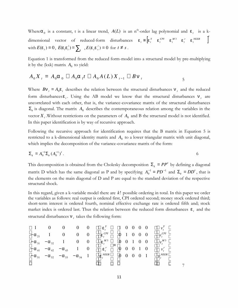
Following the recursive approach for identification requires that the B matrix in Equation 5 is

restricted to a k-dimensional identity matrix and 0A to a lower triangular matrix with unit diagonal,

which implies the decomposition of the variance-covariance matrix of the form:

)(1

0

1

0′Σ=Σ −−

AA νε . 6

This decomposition is obtained from the Cholesky decomposition PP ′=Σε by defining a diagonal

matrix D which has the same diagonal as P and by specifying 11

0

−− = PDA and DD ′=Σν , that is

the elements on the main diagonal of D and P are equal to the standard deviation of the respectivestructural shock.

In this regard, given a k-variable model there are !k possible ordering in total. In this paper we orderthe variables as follows: real output is ordered first, CPI ordered second; money stock ordered third;short-term interest is ordered fourth, nominal effective exchange rate is ordered fifth and; stock

market index is ordered last. Thus the relation between the reduced form disturbancest

ε and the

structural disturbancest

ν takes the following form:

=

−−−−−−−

−−−

NEER

t

r

t

M

t

CPI

t

Y

t

NEER

t

r

t

M

t

CPI

t

Y

t

v

v

v

v

v

33

54535251

434241

3231

21

10000

01000

00100

00010

00001

1

01

001

0001

00001

εε

εεε

ααααααα

ααα

7

12

This particular ordering has the following implications: (i) Real GDP does not reactcontemporaneously to shocks from other variables in the system. (ii) CPI does not reactcontemporaneously to shocks originating from all factors except real GDP. (iii) money stock (M3)does not react contemporaneously to real GDP but is affected contemporaneously by short-terminterest rate, nominal effective exchange rate (iv) the interest is affected contemporaneously by allshocks in the system, except those from the nominal effective exchange rate (v) nominal effectiveexchange rate is affected contemporaneously by all shocks in the system.

4 EMPIRICAL RESULTS

(a) Univariate analysis

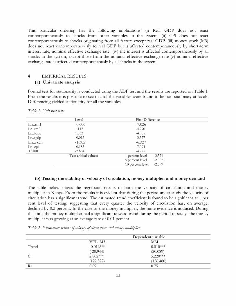
Formal test for stationarity is conducted using the ADF test and the results are reported on Table 1.From the results it is possible to see that all the variables were found to be non-stationary at levels.Differencing yielded stationarity for all the variables.

Table 1: Unit root tests

Level First Difference

Ln_rm1 -0.606 -7.026Ln_rm2 1.112 -4.790Ln_Rm3 1.332 -4.905Ln_rgdp -0.013 -3.577

Ln_exch -1.302 -6.327Ln_cpi -0.185 -7.094Tb100 -2.684 -4.775

Test critical values: 1 percent level -3.5715 percent level -2.92210 percent level -2.599

(b) Testing the stability of velocity of circulation, money multiplier and money demand

The table below shows the regression results of both the velocity of circulation and moneymultiplier in Kenya. From the results it is evident that during the period under study the velocity ofcirculation has a significant trend. The estimated trend coefficient is found to be significant at 1 percent level of testing; suggesting that every quarter the velocity of circulation has, on average,declined by 0.2 percent. In the case of the money multiplier, the same evidence is adduced. Duringthis time the money multiplier had a significant upward trend during the period of study- the moneymultiplier was growing at an average rate of 0.01 percent.

Table 2: Estimation results of velocity of circulation and money multiplier

Dependent variableVEL_M3 MM

Trend -0.016***(-20.944)

0.010***(20.089)

C 2.802***(122.322)

5.220***(126.480)

R2 0.89 0.75

13

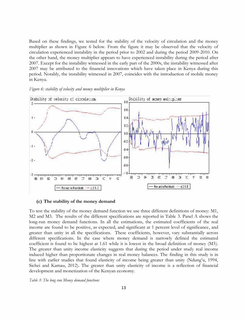
Based on these findings, we tested for the stability of the velocity of circulation and the moneymultiplier as shown in Figure 6 below. From the figure it may be observed that the velocity ofcirculation experienced instability in the period prior to 2002 and during the period 2009-2010. Onthe other hand, the money multiplier appears to have experienced instability during the period after2007. Except for the instability witnessed in the early part of the 2000s, the instability witnessed after2007 may be attributed to the financial innovations which have taken place in Kenya during thisperiod. Notably, the instability witnessed in 2007, coincides with the introduction of mobile moneyin Kenya.

Figure 6: stability of velocity and money multiplier in Kenya

(c) The stability of the money demand

To test the stability of the money demand function we use three different definitions of money: M1,M2 and M3. The results of the different specifications are reported in Table 3. Panel A shows thelong-run money demand functions. In all the estimations, the estimated coefficients of the realincome are found to be positive, as expected, and significant at 1 percent level of significance, andgreater than unity in all the specifications. These coefficients, however, vary substantially acrossdifferent specifications. In the case where money demand is narrowly defined the estimatedcoefficient is found to be highest at 1.61 while it is lowest in the broad definition of money (M3).The greater than unity income elasticity suggests that during the period under study real incomeinduced higher than proportionate changes in real money balances. The finding in this study is inline with earlier studies that found elasticity of income being greater than unity (Ndung’u, 1994,Sichei and Kamau, 2012). The greater than unity elasticity of income is a reflection of financialdevelopment and monetization of the Kenyan economy.

Table 3: The long run Money demand functions

14

Dependent variable Ln_rm1 Ln_rm2 Ln_rm3Ln_RGDP 1.610***

(26.938)1.067***(15.720)

1.011***(16.017)

Tb100 -1.289***(-4.998)

-0.037(-0.124)

-0.216(-0.964)

Ln_exc -- -- -0.396***(-3.167)

R2 0.94 0.84 0.91Dw 1.56 0.54 0.86*** significant at 1%, ** significant at 5%, * significant at 10%; (…) t-values and [ ..] critical values.

The estimated coefficient of interest rate is found to be negative in all specifications. In the case ofthe narrow definition of money, it is found to be negative and significant at 1 percent level ofsignificance. However, in the estimations involving M2 and M3, the estimated coefficients are foundto be negative but not statistically significant at the conventional levels of testing. Because the broadmoney supply includes the foreign exchange holding, it is therefore estimated with exchange rate asone of its explanatory variables. In this formulation, the coefficient of exchange rate is found to benegative, as expected, and significant at 1 percent level of testing. This finding suggests thatmovements in the exchange rate have a significant impact on the demand for broad money inKenya. That is, currency depreciation increases the demand for money as foreign currency depositliabilities increase in value of domestic currency. This valuation effect is likely to be compounded bythe substitution effect, as local residents shift from local currency-denominated deposits to foreigncurrency denominated deposits with a weakening currency.

Table 3b: Tests for Cointegration

None -3.465***[-2.580]

-2.309***[-2.580]

-2.581***[-2.581]

Intercept -3.452***[-3.472]

-2.302[-2.576]

-2.667*[-2.577]

Trend and intercept -12.592***[-4.016]

-3.235***[-3.143]

-4.465***[-4.022]

*** Significant at 1%, ** significant at 5%, * significant at 10%; (…) t-values and [ ..] critical values.

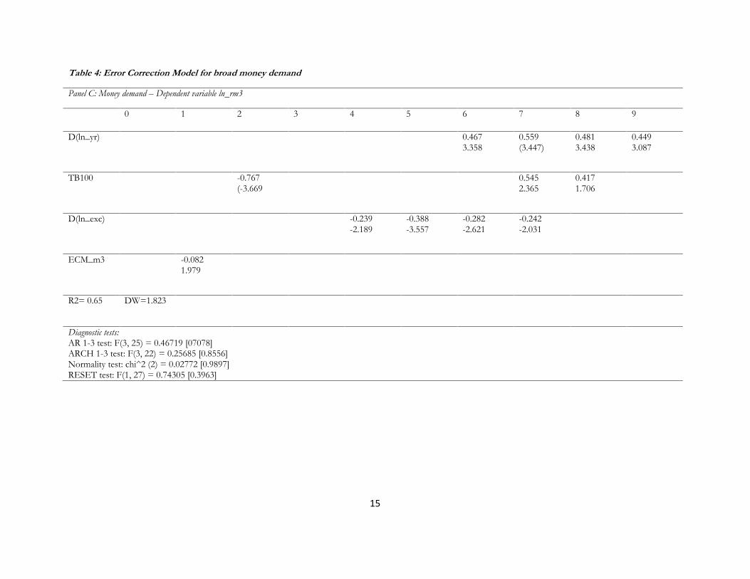
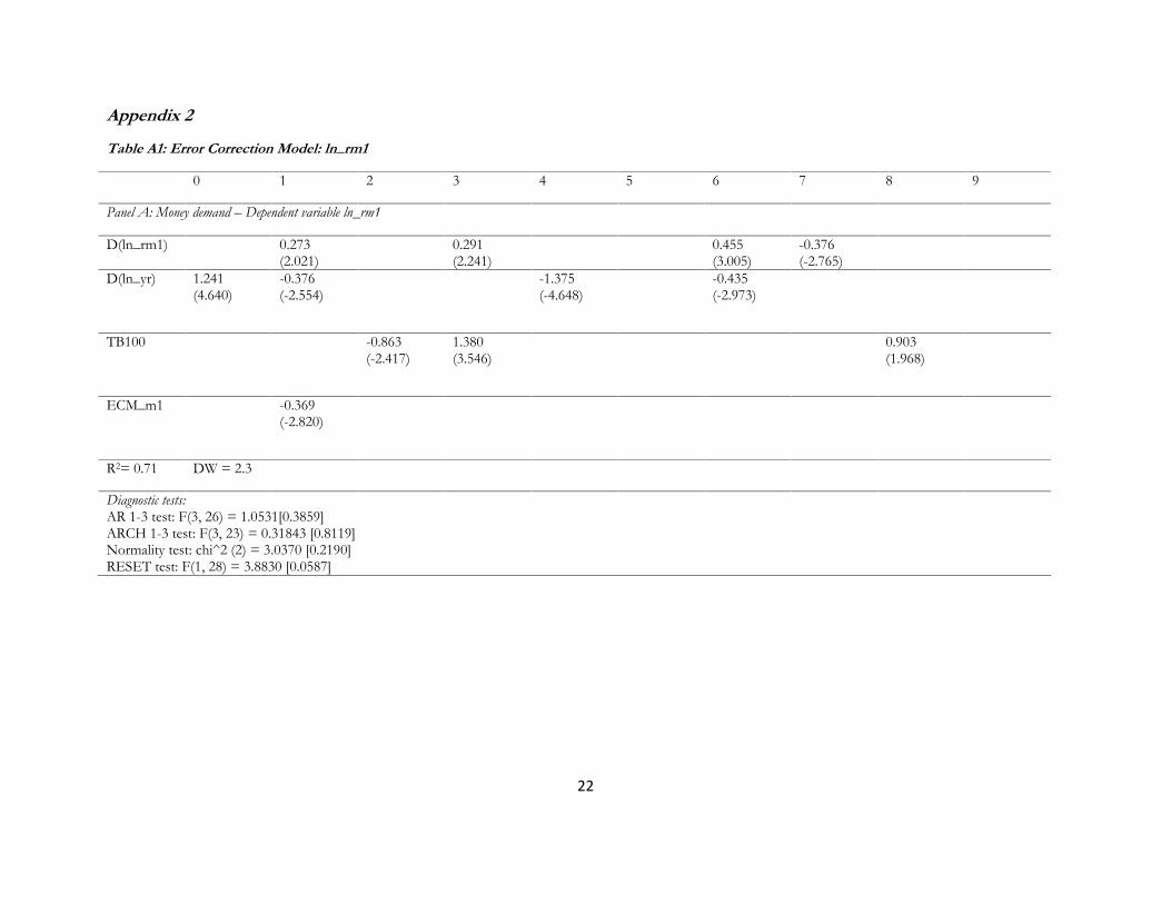
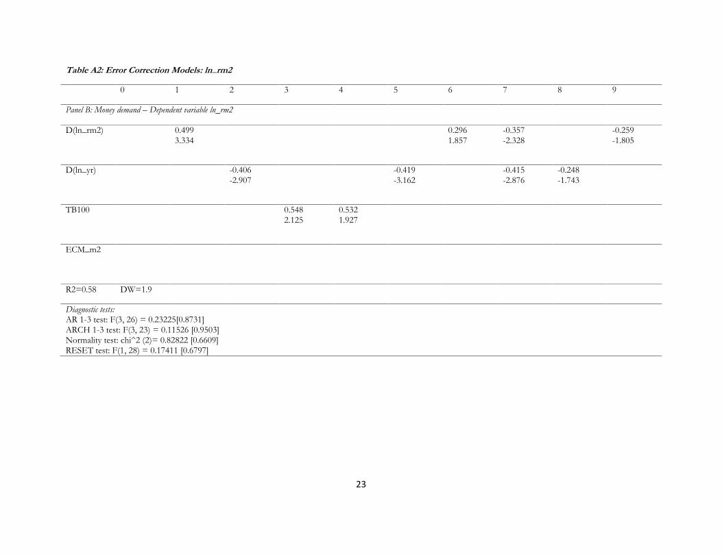
Table 3b shows the results of the cointegration test. The variables in the money demand functionsare cointegrated. Therefore we proceed to estimate the error correction models for each of the long-run demand functions as shown on Table 4 and Table A1 and A2 in the appendix. A number oftests were conducted on the error correction models reported. Statistically the respective ECMsappear well specified; there is no evidence of serial correlation (AR test), autoregressiveheteroscedasticity (ARCH test), non-normal errors (Normality test) and regression misspecification(RESET test). Based on the error correction models, it is found that in the case where the moneydemand is narrowly defined (M1), the error correction term is negative and significant at theconventional levels of testing. The estimated ECM is -0.369. In the case where money is defined asM2 and M3 the estimated ECM terms are found to be negative and also significant. However, thespeed of adjustment appears to be low at -0.06 for M2 and -0.082 for M3.

15

Table 4: Error Correction Model for broad money demand

Panel C: Money demand – Dependent variable ln_rm3

0 1 2 3 4 5 6 7 8 9

D(ln_yr) 0.4673.358

0.559(3.447)

0.4813.438

0.4493.087

TB100 -0.767(-3.669

0.5452.365

0.4171.706

D(ln_exc) -0.239-2.189

-0.388-3.557

-0.282-2.621

-0.242-2.031

ECM_m3 -0.0821.979

R2= 0.65 DW=1.823

Diagnostic tests:AR 1-3 test: F(3, 25) = 0.46719 [07078]ARCH 1-3 test: F(3, 22) = 0.25685 [0.8556]Normality test: chi^2 (2) = 0.02772 [0.9897]RESET test: F(1, 27) = 0.74305 [0.3963]

16

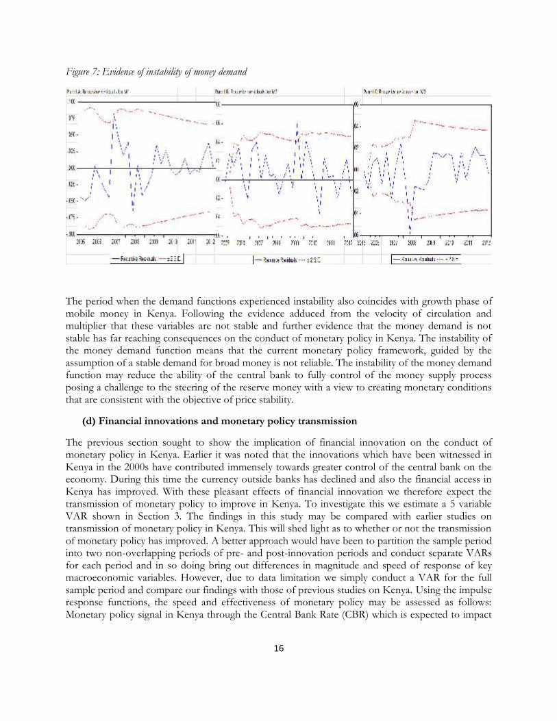
Figure 7: Evidence of instability of money demand

The period when the demand functions experienced instability also coincides with growth phase ofmobile money in Kenya. Following the evidence adduced from the velocity of circulation andmultiplier that these variables are not stable and further evidence that the money demand is notstable has far reaching consequences on the conduct of monetary policy in Kenya. The instability ofthe money demand function means that the current monetary policy framework, guided by theassumption of a stable demand for broad money is not reliable. The instability of the money demandfunction may reduce the ability of the central bank to fully control of the money supply processposing a challenge to the steering of the reserve money with a view to creating monetary conditionsthat are consistent with the objective of price stability.

(d) Financial innovations and monetary policy transmission

The previous section sought to show the implication of financial innovation on the conduct ofmonetary policy in Kenya. Earlier it was noted that the innovations which have been witnessed inKenya in the 2000s have contributed immensely towards greater control of the central bank on theeconomy. During this time the currency outside banks has declined and also the financial access inKenya has improved. With these pleasant effects of financial innovation we therefore expect thetransmission of monetary policy to improve in Kenya. To investigate this we estimate a 5 variableVAR shown in Section 3. The findings in this study may be compared with earlier studies ontransmission of monetary policy in Kenya. This will shed light as to whether or not the transmissionof monetary policy has improved. A better approach would have been to partition the sample periodinto two non-overlapping periods of pre- and post-innovation periods and conduct separate VARsfor each period and in so doing bring out differences in magnitude and speed of response of keymacroeconomic variables. However, due to data limitation we simply conduct a VAR for the fullsample period and compare our findings with those of previous studies on Kenya. Using the impulseresponse functions, the speed and effectiveness of monetary policy may be assessed as follows:Monetary policy signal in Kenya through the Central Bank Rate (CBR) which is expected to impact

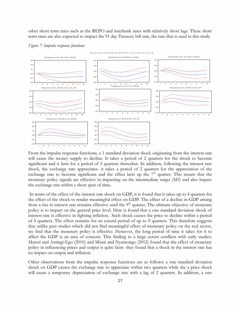
17

other short term rates such as the REPO and interbank rates with relatively short lags. These shortterm rates are also expected to impact the 91 day Treasury bill rate, the rate that is used in this study.

Figure 7: Impulse response functions

-.04

-.02

.00

.02

.04

1 2 3 4 5 6 7 8 9 10

R esponse of LN _YN _SA to T B100

-.04

-.02

.00

.02

.04

1 2 3 4 5 6 7 8 9 10

R esponse of LN _C PI to T B100

-.02

-.01

.00

.01

.02

.03

1 2 3 4 5 6 7 8 9 10

R esponse of LN _M 3_SA to T B100

-.02

-.01

.00

.01

.02

.03

1 2 3 4 5 6 7 8 9 10

R esponse of T B100 to LN _YN _SA

-.02

-.01

.00

.01

.02

.03

1 2 3 4 5 6 7 8 9 10

R esponse of T B100 to LN _N EER

-.04

-.02

.00

.02

.04

1 2 3 4 5 6 7 8 9 10

R esponse of LN _N EER to LN _YN _SA

-.04

-.02

.00

.02

.04

1 2 3 4 5 6 7 8 9 10

R esponse of LN _N EER to LN _C PI

-.04

-.02

.00

.02

.04

1 2 3 4 5 6 7 8 9 10

R esponse of LN _N EER to T B100

R e s p o n s e t o C h o le s k y O n e S . D . In n o v a t io n s ± 2 S . E .

From the impulse response functions, a 1 standard deviation shock originating from the interest ratewill cause the money supply to decline. It takes a period of 2 quarters for the shock to becomesignificant and it lasts for a period of 3 quarters thereafter. In addition, following the interest rateshock, the exchange rate appreciates- it takes a period of 2 quarters for the appreciation of theexchange rate to become significant and the effect lasts up the 7th quarter. This means that themonetary policy signals are effective in impacting on the intermediate target (M3) and also impactthe exchange rate within a short span of time.

In terms of the effect of the interest rate shock on GDP, it is found that it takes up to 4 quarters forthe effect of the shock to render meaningful effect on GDP. The effect of a decline in GDP arisingfrom a rise in interest rate remains effective until the 9th quarter. The ultimate objective of monetarypolicy is to impact on the general price level. Here is found that a one standard deviation shock ofinterest rate is effective in fighting inflation. Such shock causes the price to decline within a periodof 4 quarters. The effect remains for an extend period of up to 9 quarters. This therefore suggeststhat unlike past studies which did not find meaningful effect of monetary policy on the real sector,we find that the monetary policy is effective. However, the long period of time it takes for it toaffect the GDP is an area of concern. This finding to a large extent conflicts with early studies:Mutoti and Antingi-Ego (2010) and Misati and Nyamongo (2012) found that the effect of monetarypolicy in influencing prices and output is quite faint- they found that a shock in the interest rate hasno impact on output and inflation.

Other observations from the impulse response functions are as follows: a one standard deviationshock on GDP causes the exchange rate to appreciate within two quarters while the a price shockwill cause a temporary depreciation of exchange rate with a lag of 2 quarters. In addition, a one

18

standard deviation shock arising from exchange rate will cause immediate interest rate (policy rate aswell) rise to stem further depreciation of the currency while a GDP shock will occasion interest rateto rise as well to contain upward pressures on inflation.

Unlike past studies which established no effect of monetary policy on the real sector the currentstudy establishes that the monetary policy has started to show evidence of effectiveness. What is ofconcern, however, is the speed at which the monetary policy impacts on the real sector. This currentevidence may be on account of the recent financial developments and innovations expoundedabove.

5.0 CONCLUSIONS AND RECOMMENDATIONS

The purpose of this study was to investigate the effect of financial innovation on monetary policy inKenya during the period 1998-2012. During this period it is found that the financial sector hasdeveloped impressive and also a number of financial innovations have taken place in the country:the number of bank branches and Automated Teller Machines has increased; mobile money as wellas agency banking innovation has been witnessed during this period. Following these developmentsthe proportion of the population outside the banking system has declined substantially and also thecurrency outside banks has dwindled over time. The study results point to improved effectivenessof monetary policy. While earlier studies found no significant effect of monetary policy on the realsector, this analysis shows for instance that an interest rate shock impacts on GDP within 4 quartersand the effect remains effective until the 9th quarter. This finding is in line with studies that showthat innovations strengthen the interest rate channel.

However, these innovations have come at a cost. The velocity of money, the money multiplier andthe money demand have become unstable. This has implications on the monetary targetingframework for Kenya. However, there are indications that these relationships are stabilizing in thevery recent past. This shows there is need for keep a keen check on evolution these relationships soas to disentangle monetary evolutions that may reflect structural changes from those that may beshort-run monetary developments. Such monitoring can, for instance, allow adjustments to be madeto monetary aggregates in case of transitory shocks, in order to account for portfolio shifts whichimpact the demand for money without any incidence on future inflation. A permanent shift may,however, mean a change in the current monetary policy framework and adoption of more a flexibleone. A possible candidate could be inflation targeting which is less restrictive.

Nevertheless, the financial innovations initiatives have had a positive effect in view of the improvedefficiency of the monetary transmission mechanism and enhanced financial deepening and should besupported.

19

References

Al-Laham, M., Al-Tarawneh, H. & Abdallat, N. (2009). Development of electronic money and itsimpact on the central bank role and monetary policy. Issues in Informing Science andInformation Technology, 6: 339-349.

Angeloni I., A. Kashyao and B. Mojon (ed) (2003), Monetary Policy Transmission in the Euro Area,Cambridge university Press.

Arrau, P. & De Gregorio, J. (1993). Financial innovation and money demand: Application to Chileand Mexico. The Review of Economics and Statistics, 75(3): 524-530.

Awad, I. (2010). Measuring the stability of the demand for money function in Egypt. Banks andBanking Systems, 5(1):71-75.

Bert, E. (1996). "Electronic Money And Monetary Policy: Separating Fact From Fiction", CatoInstitute's Conference on The Future of Money in the Information Age,May 23, 1996

Cho, D & Miles, W. (2007). Financial innovation and the stability of money demand in Korea.Southwestern Economic Review, 34(1): 51-60.

Freedman, C., (2006) "Monetary Policy Implementation: Past, Present and Future: Will the Adventof Electronic Money Lead to the Demise of Central Banking?" Future of Monetary Policyand Banking Conference, Washington D.C, July, 11, 2000

Friedman, B. M. (1999): The future of Monetary Policy : The central Bank as an Army with only asingle Corps? International Finance, 2 (3).

Gurley, J.G. & Shaw, E.S. (1960). Money in a Theory of Finance. Brookings Institution,Washington D.C.

Hasan, M. (2009). Financial innovations and the interest rate elasticity of money demand in theUnited Kingdom, 1963-2009. International Journal of Business and Economics, 8(3): 225-242.

Hughes, N. & Lonie, S. (2007). M-PESA: Mobile money for the “Unbanked” Turning cellphonesinto 24-hour tellers in Kenya. Journal of Innovations: Technology, Government,Globalization, 2(1-2): 63-81.

Kobrin, Stephen J. (1997), "Electronic Cash and the End of National Markets," Foreign Policy 107(Summer), 65-77.

20

Khemraj, T. (2008). Excess liquidity, oligopolistic loan markets and monetary policy in LDCs. DESPWorking Paper, 64

Kovanen, A. (2004), “Zimbabwe: A quest for a nominal anchor”, IMF Working Paper, WP/04/130

Lungu, M., Simwaka, K & Chiumia, A. (2012). Money demand function for Malawi-implications formonetary policy conduct. Banks and Bank Systems. 7(1): 50-63.

McKinnon, R. (1973). Money and Capital in Economic Development. The Brookings Institution,Washington.

Misati, R. N. & Nyamongo, E. M. (2012). Asset prices and monetary policy in Kenya. Journal ofEconomic Studies, 39(4): 451-468.

Mwega, F.M. (1990). An Econometric study of monetary policy in Kenya. ODI working paper, 42.

Noyer, C, 2006. “Does money matter? A European perspective”, at the 4th ECB Central BankingConference “The role of money: money and monetary policy in the twenty-first century”,Frankfurt am Main, 9 November 2006.

Noyer, C. 2007. “Financial Innovation, Monetary Policy and Financial Stability”, Spring Conferenceof the Bank of France/Deutsche Bundesbank, Eltville, Germany, April 2007.

Saif S. Al-Sowaidi, S.S and A. F. Darrat. 2006. “Financial Innovations and the Stability of LongrunMoney Demand: Implications for the Conduct of Monetary Policy in Three GCC Countries

Sichei, M. & Kamau, A. (2012). Demand for money: Implications for the conduct of monetarypolicy in Kenya. International Journal of Economics and Finance, 4(8): 72-82.

Viren, M. (1992). Financial innovations and currency demand: Some new evidence. EmpiricalEconomics, 17(4): 451-461.

Weil, D., Mbithi, I & Mwega, F. (2012). The implications of innovations in the financial sector onthe conduct of monetary policy in East Africa. Report submitted to the InternationalGrowth Centre Tanzania Country Program.

21

Appendix 1

Figure A1: Evolution of bank branches and ATMs in Kenya: 2000-2011

Source: Central Bank of Kenya, Bank Supervision annual reports.

22

Appendix 2

Table A1: Error Correction Model: ln_rm1

0 1 2 3 4 5 6 7 8 9

Panel A: Money demand – Dependent variable ln_rm1

D(ln_rm1) 0.273(2.021)

0.291(2.241)

0.455(3.005)

-0.376(-2.765)

D(ln_yr) 1.241(4.640)

-0.376(-2.554)

-1.375(-4.648)

-0.435(-2.973)

TB100 -0.863(-2.417)

1.380(3.546)

0.903(1.968)

ECM_m1 -0.369(-2.820)

R2= 0.71 DW = 2.3

Diagnostic tests:AR 1-3 test: F(3, 26) = 1.0531[0.3859]ARCH 1-3 test: F(3, 23) = 0.31843 [0.8119]Normality test: chi^2 (2) = 3.0370 [0.2190]RESET test: F(1, 28) = 3.8830 [0.0587]

23

Table A2: Error Correction Models: ln_rm2

0 1 2 3 4 5 6 7 8 9

Panel B: Money demand – Dependent variable ln_rm2

D(ln_rm2) 0.4993.334

0.2961.857

-0.357-2.328

-0.259-1.805

D(ln_yr) -0.406-2.907

-0.419-3.162

-0.415-2.876

-0.248-1.743

TB100 0.5482.125

0.5321.927

ECM_m2

R2=0.58 DW=1.9

Diagnostic tests:AR 1-3 test: F(3, 26) = 0.23225[0.8731]ARCH 1-3 test: F(3, 23) = 0.11526 [0.9503]Normality test: chi^2 (2)= 0.82822 [0.6609]RESET test: F(1, 28) = 0.17411 [0.6797]