Federal Reserve Bank of Dallas Globalization and Monetary Policy Institute

Working Paper No. 52 http://www.dallasfed.org/assets/documents/institute/wpapers/2010/0052.pdf

Financial Globalization, Financial Frictions and

Optimal Monetary Policy*

Ester Faia Goethe University Frankfurt

Kiel IFW CEPREMAP

Eleni Iliopulos

PSE University of Paris 1

CEPREMAP

June 2010

Abstract How should monetary policy be optimally designed in an environment with high degrees of financial globalization? To answer this question we lay down an open economy model where net lending toward the rest of the world is constrained by a collateral constraint motivated by limited enforcement. Borrowing is secured by collateral in the form of durable goods whose accumulation is subject to adjustment costs. We demonstrate that, although this economy can generate persistent current account deficits, it can also deliver a stationary equilibrium. The comparison between different monetary policy regimes (floating versus pegged) shows that the impossible trinity is reversed: a higher degree of financial globalization, by inducing more persistent and volatile current account deficits, calls for exchange rate stabilization. Finally, we study the design of optimal (Ramsey) monetary policy. In this environment the policy maker faces the additional goal of stabilizing exchange rate movements, which exacerbate fluctuations in the wedges induced by the collateral constraint. In this context optimality requires deviations from price stability and calls for exchange rate stabilization. JEL codes: E52, F1

* Ester Faia, Chair in Monetary and Fiscal Policy, Goethe-Universität Frankfurt am Main, Senckenberganlage 31, 60325 Frankfurt am Main, Germany. faia@wiwi.uni-frankfurt.de. Eleni Iliopulos, Paris School of Economics, University of Paris 1 Panthéon – Sorbonne, MSE, bureau 309, Bd L'Hôpital 75647, Paris CEDEX 13, France. 0033-0-1-44-07-82-65. Eleni.iliopulos@univ-paris1.fr. We gratefully acknowledge financial support from European Community grant MONFISPOL under grant agreement SSH-CT-2009-225149. We thank participants at the MONFISPOL Meeting held in Pairs and to the conference "Theory and Methods in Macroeconomics" for comments. The views in this paper are those of the authors and do not necessarily reflect the views of the Federal Reserve Bank of Dallas or the Federal Reserve System.

1 Introduction

The last two decades have been characterized by an extraordinary wave of �nancial globalization

often accompanied with persistent current account imbalances1. For many countries current account

imbalances have been negatively related to booms in house price, mortgages and consumer credits

and durable demand. Since a signi�cant proportion of claims on consumers credit has been placed

in the international markets, for many countries the boom in durable demand has been mainly

�nanced with foreign lending2. Lending standards have been in general quite loose along several

dimensions and overall they have been tied to collateral values, in a way that swings (upward or

downward) in durable prices (particularly house prices) have determined the amount of lending3.

Against this background many central banks around the world have followed, explicitly or

implicitly, in�ation targeting or price stability polices without putting any weight on asset or durable

prices and exchange rate movements. This is remarkable given that some countries had experienced

signi�cant exchange rate depreciations and asset price growth. We therefore ask whether the

prescriptions for monetary policy change in an environment as the one described above.

To this purpose we lay down a DSGE small open economy model in which agents consume

durable and non-durable goods4, supply labour services and �nance consumption with foreign

lending. The rest of the world is populated by in�nite lived agents who behave as consumption

smoothers. Total (net) lending is constrained by a borrowing limit and is secured by collateral

in the form of durable stock, as the latter can be seized by lenders in the event of default. Due

to imperfect monitoring only a fraction of this collateral can be pledged by lenders. The type of

borrowing constraint considered is a collateral constraint on the line of Kiyotaki and Moore [46],

Kocherlacota [48], Chari, Kehoe and McGrattan [23] among others. We further assume that durable

goods provide utility services (see Davis and Heatcote [29], Miles [64], Iacoviello [41], Campbell

1Backus, Henriksen, Lambert, Telmer [5] show that among industrialized countries the US, the UK, Spain andAustralia have run persistent current account de�cits.

2See Bernanke [15] for a discussion of the link between global imbalances and house price booms. He noticedthat countries whose current accounts have moved toward de�cit have generally experienced substantial housingappreciation and increases in household wealth.

3The collateral policy practice adopted in the last two decades were quite risky as absence of any informationon future income streams the availability of lending is heavily dependent on the market swings. In many occasionsbanks have renewed and replenished mortgages whenever the house price had gone up independently from the abilityof the borrower to repay.

4We assume that only non-durable goods are tradable and are aggregated through Armington aggregator.

2

and Hercowitz [19] and Monacelli [65]) and that durable investment is subject to adjustment costs,

an assumption which allows to reproduce persistence in response to various shocks (see Topel

and Rosen [83], Erceg and Levin [33]). In this model net asset accumulation is determined by

the borrowing constraint and depends on the future value of collateral. The degree of �nancial

globalization in this economy is captured by the parameter characterizing the sensitivity of foreign

lending to the value of collateral, as a higher value relaxes the constraint on foreign lending.

There are two production sectors in the domestic economy: the durable good sector and the non-

durable goods sector. Firms in both sectors are monopolistic competitive and face Rotemberg

[75] adjustment costs: this assumption is introduced to study non-neutral monetary policy and to

compare alternative monetary policy regimes. Monetary policy is conducted by means of Taylor

type rules.

Three results arise. First, we show that the net asset accumulation in this model is uniquely

determined in the steady state and that it is saddle path stationary in a neighborhood of the

steady state. A crucial assumption for this result is that foreign agents have higher discount rates

than domestic lenders. In this case the domestic economy experiences a persistent current account

de�cit, as in equilibrium domestic residents behave as impatient agents and borrow from the rest

of the world. Despite this, the current account de�cit leads to stationary dynamics. Second, we

compare alternative monetary policy regimes (�oating versus pegged) under productivity, govern-

ment expenditure and global liquidity shocks and for alternative degrees of �nancial globalization.

Our �ndings show that the impossible trinity is reversed in this model: higher degree of �nancial

liberalization exacerbate the destabilizing e¤ect of exchange rate �uctuations on foreign debt, con-

sumption and output, hence it calls for more aggressive exchange rate targeting. Third, we analyze

the trade-o¤s faced by the policy maker in this environment and derive the optimal (Ramsey)

plan. The design of optimal policy is conducted in two steps. First, we lay down analytically

the conditions that characterize the constrained pareto optimal allocation for the model economy

under �exible prices; this allows us to highlight the role of real wedges in our economy. Second, we

analyze the quantitative properties of the Ramsey plan for the economy with sticky prices. We �nd

that monetary policy should deviate from price stability and smooth exchange rate �uctuations,

the more so the higher the degree of �nancial liberalization. The Ramsey planner faces a trade o¤

3

between stabilizing domestic prices, both in the durable and the non-durable sector, as this serves

the goal of closing the price adjustment costs, and stabilizing �uctuations in the exchange rate.

Movements in the latter, indeed, tend to amplify the �uctuations of the wedges, induced by the

presence of the collateral constraint, on both, the marginal rate of substitution between durable and

non-durable consumption and the marginal rate of substitution between non-durable consumption

at two di¤erent dates. Through those channel, indeed, �nancial globalization can amplify ine¢ cient

�uctuations in consumption. The �rst of those two goals is achieved by targeting solely domestic

in�ation, while the second requires exchange rate targeting. The second motive tends to prevail,

the more so in presence of increasing �nancial openness.

The rest of the paper proceeds as follows. Section 2 presents the model. Section 3 demonstrates

how to obtain a stationary equilibrium. Section 4 describes the transmission mechanism in this

model. Section 5 shows the comparison of alternative monetary policy regimes under alternative

degree of �nancial liberalization. Section 6 shows the results of the optimal policy plan. Section 7

concludes.

2 Related Literature

Our paper contains both positive and normative results and because of this it is related to several

strands of the literature.

In the open economy literature borrowing limits have been used to analyse various issues such

as sudden stops (see Mendoza [61], Chari et al. [22]), over-borrowing (see Uribe [84], Benigno et

al. [14]), global imbalances (see Mendoza et al. [63]), macroeconomic volatility (see Perri and

Quadrini [69]) and welfare gains from �nancial integration (see Mendoza et al. [62], Aoki et al.

[2]). All those studies analyze borrowing constraints in RBC economies and do not analyze optimal

monetary policy. Additionally all those studies focus on borrowing constraints, in which physical

capital or other forms of pleadable income play the role of collateral. An exception is given by

Iacoviello and Minetti[42], who introduce in an RBC model a constraint with housing collateral to

explain output co-movements across countries. This paper, on the contrary, considers the role of

durable goods as collateral. The reason for the latter modeling assumption comes from the fact

that there is signi�cant evidence that consumers�loans require the borrower to post some collateral

4

and that housing or durable goods represent, in most economies, the largest form of collateral (see

Black et al. [17] and Attanasio et al. [4]).

In the open economy literature other papers have studied the e¤ects of �nancial globalization

(see Broner and Ventura [18], Devereux and Sutherland [32]) and its link with monetary policy

(Devereux and Sutherland [32]). Most papers have modelled �nancial globalization in the form of

international portfolio asset allocation, while we focus on collateral constrained lending.

The stabilization properties of alternative exchange rate regimes have been studied in sev-

eral other papers, which introduce �nancial frictions in open economy models. For instance, See

Cespedes, Chang and Velasco [21], Gertler, Gilchrist and Natalucci [40], Faia [34] introduce a �-

nancial accelerator mechanism in open economy and show that �xed exchange rates can be more

destabilizing than �oating exchange rates. Lahiri, Singh and Vegh [52] challenge the standard

Mundell-Fleming prescription by showing that in presence of segmented asset markets �oating

exchange rate regimes perform better than �xed exchange rates, when shocks are real, and vicev-

ersa, when shocks originate in the money market. Our paper shows that the introducing �nancial

frictions in the form of collateral constraints consistently leads to a superiority of pegging the ex-

change rates, the reason being that �uctuations in the exchange rate destabilize foreign lending

and, consequently, current account and consumption demand.

Our paper also analyzes the design of optimal monetary policy and the scope for exchange

rate targeting. In this respect our work is related to a strand of the open economy literature which

studies optimal monetary policy. The classical analysis in Clarida, Gali and Gertler [25] and Gali

and Monacelli [38] concludes that optimal monetary in a open economy models should target solely

producer price in�ation. The rationale for such an inward looking strategy comes from proving

the isomorphism between the competitive equilibrium relations characterizing the closed and the

open economy models. In this context the scope for exchange rate stabilization is absent. The

limited role for exchange rate targeting is con�rmed in Devereux and Engel [31], who, by reviving a

popular argument due to Friedman [36], assert that in the presence of price stickiness, exchange rate

movements should be instrumental to have the economy replicate the allocation under purely �exible

prices, which implies maintaining constant mark-ups. A motive for deviating from strict markup

stabilization generally lies in the possibility of strategically a¤ecting the terms of trade (the relative

5

price of imports). A terms of trade variation, by altering domestic residents�purchasing power,

a¤ects consumption for any given level of output (labor e¤ort). Previous contributions, Corsetti and

Pesenti [27], Sutherland [82], Benigno and Benigno [12], have shown that this terms-of-trade motive

vanishes if either of two conditions holds: (i) the intratemporal elasticity of substitution between

domestic and imported goods is unitary; (ii) that same elasticity coincides with the intertemporal

elasticity of substitution in consumption. More recently Faia and Monacelli [35] have shown that

in a small open economy with home bias the policy maker will optimally deviate from an inward

looking strategy and will target the exchange rate. Under home bias, variations in the terms of

trade induce also variations in the real exchange rate , which, in turn, a¤ect domestic consumption

via international risk-sharing (for any given level of foreign consumption). In the present paper,

we show that in an economy with incomplete international markets and collateral constraints on

external debt, there is an additional and independent motive for exchange rate targeting, namely

the need for stabilizing �uctuations in external debt. Later indeed we show that exchange rate

movements exacerbate the �uctuations on the wedges induced by the collateral constraint.

3 A Small Open Economy with Collateral Constraints

There is a small open economy (which we refer to as the domestic economy) and the rest of the

world. A crucial assumption in our set-up is that residents of the small open economy have lower

discount factors compared to agents populating the rest of the world. As domestic agents are

impatient, in equilibrium the small open economy will have a negative asset position; we will

return on this point later.

The small open economy is populated by in�nitely lived agents who consume non-durable and

durable goods, work, invest in domestic government claims and require loans to �nance expendi-

tures. Consumption in durable and non-durable goods is �nanced through foreign lending, which

takes the form of non�state contingent securities and is bounded above by a fraction of the future

value of the collateral - i.e. durable goods. Because of this, the net asset position, both in the long

and in the short run, is linked to the future value of collateral. Demand for durable goods is justi�ed

since they enter the utility function. The assumption of a �nancially constrained open economy is

justi�ed by the inability of foreign lenders to implement perfect monitoring. Under those circum-

6

stances the tightness of the borrowing limit depends on the degree of information asymmetry, of

�nancial market integration and of debt repossession ability which in turn depends upon legal and

institutional arrangements. There are two production sectors in this economy: the durable good

sector and the non-durable goods sector. Firms in both sectors are monopolistic competitive and

face Rotemberg [75] adjustment costs.

3.1 Domestic Households

Let st = fs0; ::::stg denote the history of events up to date t, where st denotes the event realization

at date t. The date 0 probability of observing history st is given by �t. The initial state s0

is given so that �(s0) = 1: Henceforth, and for the sake of simplifying the notation, let�s de�ne

the operator Etf:g �P

st+1�(st+1jst) as the mathematical expectations over all possible states of

nature conditional on history st:

Agents maximize the following expected discounted sum of utilities:

Et

( 1Xt=0

�tU(CI;t; Nt)

)(1)

where total labour hours are denoted with Nt, total aggregate consumption is denoted by:

CI;t =

(1� )

1�C

��1�

t + 1�

�Dt

��1�

! ���1

(2)

where PI;t � [(1� )P 1��t + P 1��d;t ]1

1�� ; Pt is the aggregate price index for non-durable consumption

and Pd;t is the aggregate price index for durable consumption. Non-durable consumption is given

by a Dixit-Stiglitz consumption aggregator of domestic and imported goods (with � being the

intratemporal elasticity):

Ct =

��1�C

��1�

h;t + (1� �)1�C

��1�

f;t

� ���1

(3)

and durable consumption given by:

�Dt = Dt�1 �

2

(Xt � �Dt�1)2

Dt�1(4)

where Dt�1 is the real value of the stock of durable goods which is held in positive amount for it

generates utility, Xt = Dt � (1� �)Dt�1 is investment in durable goods, � is the depreciation rate

7

and the function 2 (

Xt��Dt�1Dt�1

)2 represents an adjustment cost function. Preferences are concave,

bounded above and satisfy Inada conditions and � represents the discount factor of domestic

agents. As domestic residents are impatient we assume that � < �;with � being the discount factor

of foreign residents.

Afert de�ning Pt � [�P 1��h;t +(1��)P 1��f;t ]1

1�� as the domestic price index and St =Pf;tPh;t

as the

terms of trade; optimal demands for domestic and imported goods imply the following relation:

Ch;tCf;t

=�

(1� �)(St)� (5)

The household receives at the beginning of time t a labor income of WtNt, where Wt is the

nominal wage. Agents can invest in domestic (nominal) government claims, Bt; which pay a gross

nominal interest rate one period later. Furthermore, they can borrow in foreign currency, B�t . The

gross nominal interest rate to be paid on foreign borrowing is given by R�nt : Agents can also buy and

sell durables, Dt; in an internal competitive market5. Agents are also owners of the monopolistic

sectors which produce durable and non-durable goods, hence they receive pro�ts �d;t and �h;t.

The price of durable in terms of consumption goods is denoted Zt =Pd;tPt: Finally, agents pay lump

sum transfers, � t:

The sequence of budget constraints in nominal terms reads as follows:

PtCt�Rnt�1Bt�1+etRn;�t�1B

�t�1+PtZt (Dt �Dt�1(1� �)) �WtNt�Bt+etB�t +� t+�h;t+�d;t (6)

where et is the nominal exchange rate. It is now convenient to re-state the budget constraint

in real terms:

Ct �Rnt�1bt�1�t

+Rn;�t�1etet�1

b�t�1�t

+Zt (Dt �Dt�1(1� �)) =Wt

PtNt � bt + b�t +

� tPt+�h;tPt

+�d;tPt

(7)

where etB�tPt= b�t are real international bonds and

BtPt= bt are real domestic bonds. The crucial

assumption in this model is that agents face borrowing constraints on the world market. As the

foreign lenders are not able to fully repossess their funding, debt and its services are guaranteed

as repayable up to a certain fraction of the collateral value (limited liability constraint). The

5As the bigger fraction of durables is represented by residential housing, non-tradability is an empirically plausibleassumption.

8

collateral corresponds to the future value of the durable good Pt+1Zt+1Dt. To formalize this idea

let´s assume that domestic households face the following period-by-period borrowing constraint on

foreign nominal debt:

R�nt B�t � Etf

Pt+1et+1

Zt+1Dtg (8)

which states that the debt repayment service in foreign currency (the currency of the lender),

needs to be less or equal to the expected foreign-currency value of the collateral. Constraint 8 can

arise in presence of limited enforcement without default6. In equilibrium debt repudiation never

occurs as the lender would repossess the whole collateral value. Collateral is in fact used as a

promise for repayment. The parameter is the fraction of the future value of the collateral that is

guaranteed to be repaid and can be interpreted as a down payment. Hence re�ects the degree of

information asymmetry, of �nancial market integration and of debt repossession ability of foreign

lenders which in turn depends upon legal and institutional arrangements. In general it is assumed

that it is costly for foreign lenders to repossess the entire collateral value. Since increasing allows

to relax the borrowing limit and to increase the availability of foreign lending, we assume that

higher degree of �nancial liberalization is associated with higher value of :

Once again it is convenient to re-state the constraint in real terms:

Rn;�t b�t � Etf�t+1Zt+1Dt

et+1et

g (9)

where etB�tPt= b�t are real international bonds. From equation 9 it is clear that �uctuations in

the real exchange rate in�uence the link between collateral and net asset accumulation: a real ex-

change rate depreciation can increase the value of collateral and ease the borrowing constraint. Let�s

assume that assume a separable utility. Households choose the set of processes fCt; Nt; bt; b�t ; Dtg1t=0

taking as given the set of processes fPt; Wt; Rnt ; R

n�t ; Ztg1t=0 and the initial wealth b0; b�0; D0 so as

to maximize 1 subject to7 and 9. Let�s de�ne Uc;t�t as the lagrange multiplier on 9: The following

optimality conditions must hold:

Uc;tWt

Pt= �Un;t (10)

6Perri [70] in the New Palgrave Dictionary of Economics clari�es that default occurs in equilibrium when limitedenforcement is coupled with other frictions.

9

Uc;t = �Et

�Rnt�t+1

Uc;t+1

�(11)

Uc;t �Rn�t �tUc;t = �Et

�Uc;t+1

et+1et

Rn�t�t+1

�(12)

ZtUc;t � Uc;t�tEt

(�t+1Zt+1

et+1et

)+ U �

Dt (Dt �Dt�1Dt�1

) (13)

= Et

��U �

Dt+1(1 + (

Dt+1 �Dt

Dt) +

2

(Dt+1 �Dt)2

D2t

)

�+ (1� �) �Et fZt+1Uc;t+1g

Equation 10 gives the optimal choice of labor supply. Note that in this context the borrowing

constraint does not a¤ect directly the marginal rate of substitution between consumption and

leisure. Equation 11 is the �rst order condition on domestic bond holding. Equation 12 is the

�rst order condition with respect to foreign bonds and it can be interpreted as a modi�ed Euler

condition; a binding borrowing constraint (which implies a positive �t) induces a intratemporal

distortion in the value of consumption between two di¤erent dates

Equation 13 is the e¢ ciency condition for the intertemporal choice of the durable good. The

intuition for this equation is as follows. The time t marginal cost of foregoing one unit of non-

durable consumption (weighted by the price of the durable) is equated to its marginal gain which

has three components. The �rst is the direct marginal utility of one additional unit of durable

investment now and in the future:

Et

��� �

Dt+1(1 + (

Dt+1 �Dt

Dt) +

2

(Dt+1 �Dt)2

D2t

�(14)

The second is the expected marginal utility of one unit of non-durable consumption postponed into

the future:

�(1� �)Et fZt+1Uc;t+1g (15)

If the agent shifts today one unit of consumption from non-durable to durable goods, by ac-

quiring more collateral, he can increase his debt availability which in turn raises future consumption

demand for non-durables.

The third component of the marginal gain is given by the shadow value of relaxing the liability

constraint, Uc;t�tEt

��t+1Zt+1

et+1et

�, as an additional unit of collateral becomes available. From equa-

tion 13 it stands clear that a binding borrowing constraint induces an intertemporal distortion of

10

magnitude Uc;t�tEt

��t+1Zt+1

et+1et

�in the value of durable consumption between two di¤erent dates.

Such wedge behaves as a tax on durable goods and changes in its magnitude can shift consumption

from durable to non-durable goods. An increase in the parameter has both a direct and an

indirect impact on this wedge. Those two e¤ects move actually in opposite directions. The direct

impact comes form the fact that the size of the wedge itself depends upon : A higher value of this

parameter increases credit availability therefore acting as a positive wealth shock that reduces the

demand for collateralizable durable goods. In other words an increase in increases the tax on

durable good, as it reduces the marginal bene�t of durable relative to non-durable at the current

date. The indirect impact comes from the fact a higher value of ; by relaxing the borrowing limit,

reduces the size of �t. As the shadow value of the borrowing limit decreases, the marginal bene�t

of one additional unit of collateral today increases. As �t enters the durable tax component; a

decrease in �t will induce agents to substitute non-durable with durable consumption goods. Later

on, our quantitative simulations will show that the �rst e¤ect tends to prevail so that, in response

to shocks, we observe an increase in the volatility of non-durable consumption and a decrease in

the volatility of durable consumption.

3.2 Foreign Households

The rest of the world can be thought as approximating a continuum of countries whose trade

balance is zero. This implies that P �f;t = P �t : Agents in the rest of the world behave as standard

consumption smoother. Let´s de�ne � as the discount factor of foreign residents. This implies that

the following consumption Euler condition holds:

Uc�;t = �Et

�R�nt��t+1

Uc�;t+1

�(16)

Nominal interest rate in the rest of the world are exogenously given; they can become time-

varying when modeled as random shocks. Furthermore foreign households face the following optimal

demand for domestic goods:

C�h;t = ��Y �t

�P �h;tP �t

���(17)

11

3.3 Open Economy Relations

It is assumed that the law of one pice holds continuously so that Ph;t = etP�h;t and Pf;t = etP

�f;t

where et is the nominal exchange rate. Given the de�nition for the terms of trade and the CPI

index, the following equation for the CPI in�ation (for non-durable goods) holds:

�t = �h;t

��+ (1� �)S1��t

� 11��

��+ (1� �)S1��t�1

� 11��

(18)

The real exchange rate is given by:

qt =h� (St)

��1 + (1� �)i 11��

= g(St) (19)

3.4 Non-durable Goods Production Sector

Firms in the non-durable production sector are monopolistic competitive and face Rotemberg [75]

adjustment costs. They produce di¤erent varieties of goods according to the following production

function:

Yt(i) = Ah;tNh;t (i)

As non-durable goods are aggregated according to the following Dixit-Stiglitz aggregators Ch;t �R 10 [Ch;t(i)

"�1" di]

""�1 and Cf;t �

R 10 [Cf;t(i)

"�1" di]

""�1 �rms face the following demand function:

Yt(i) =

�Ph;t(i)

Ph;t

��"Yt (20)

Firms choose the path of prices Ph;t (i) to maximize expected discounted future pro�ts:

E0

( 1Xt=0

�0;t

Yt(i)Ph;t (i)�WtNh;t (i)�

!

2

�Ph;t (i)

Ph;t�1 (i)� 1�2

Ph;t

!)

subject to the demand constraint in 20, with �t;t+1 � �0;t+1�0;t

� �Et

n1

1� t�t+1�t

PtPt+1

obeing the

borrower�s stochastic discount factor and with !2

�Ph;t(i)Ph;t�1(i)

� 1�2Ph;t representing �rm�s costs of

adjusting prices. The parameter ! represents slugginesh in price adjustment. Let´s de�ne mch;t as

12

the lagrange multiplier on constraint 20. After imposing symmetry and substituting for the labour

market equilibrium conditions, we obtain the following optimality condition for prices:

! (�h;t � 1)�h;t = Ah;tNh;t"

�(1� ")"

+1

Ah;t

�UN;tUT;t

h�+ (1� �)S1��t

i 11���

(21)

+!�Et

8<:�

1

1� t

�Uc;t+1Uc;t

"�+ (1� �)S1��t

�+ (1� �)S1��t+1

# 11��

(�h;t+1 � 1)�h;t+1

9=;3.5 Durable Goods Production Sector

Firms in the durable goods production sector solve a similar maximization problem than �rms in

the non-durable sector. Hence optimal pricing condition reads as follows:

!d (�d;t � 1)�d;t = Ad;tNd;t"

�(1� ")"

+1

Zt

�UN;tUc;tAd;t

�(22)

+!d�Et

��1

1� t

�Uc;t+1Uc;t

Zt+1Zt

(�d;t+1 � 1)�d;t+1�

3.6 Government Budget Constraint

There is a passive �scal authority who issues bonds to cover the budget de�cit. Hence the govern-

ment budget constraint reads as follows:

Bt �Rnt�1Bt�1 = gt � � t (23)

3.7 Market Clearing

Given that labor is immobile across countries, labor market clearing implies:

Nd;t +Nh;t = Nt (24)

For good markets to be cleared in country h; total purchases of durable goods must equalize

total domestic production:

Ad;tNd;t = Dt � (1� �)Dt�1 +!d2(�d;t � 1)2 (25)

As non-durables are traded market clearing requires that total production is equalized to

domestic and foreign demand:

13

Ah;tNh;t = �Yt

�Ph;tPt

���+ (1� �)Y �t

�P �h;tP �t

���+!

2(�h;t � 1)2 + gt (26)

where gt represents exogenous government spending and follows a AR(1) shock.

3.8 UIP and Asset Evolution

The arbitrage condition between domestic government claims and foreign bond holdings, equations

11 and 12, implies the following uncovered interest rate parity:

Rnt = R�nt

h�t + �Et

net+1et

Uc;t+1�t+1Uc;t

oih�Et

nUc;t+1�t+1Uc;t

oi (27)

The evolution of foreign debt is obtained by the aggregate budget constraint of the domestic

residents:

Ct+Zt (Dt �Dt�1(1� �))+WtNt

Pt+�h;tPt

+�d;tPt

�Rnt�1bt�1�t

+ bt�� tPt= b�t �Rn�t�1

etet�1

b�t�1�t

(28)

Substituting the expression for the pro�t functions, �h;tPt+�d;tPt; and imposing the government

budget constraint, deliver:

Ah;tNh;t�!

2(�h;t � 1)2� gt+Zt(Ad;tNd;t�

!n2(�d;t � 1)2) +

Un;tUc;t

Nt = b�t �Rn�t�1etet�1

b�t�1�t

(29)

Equations 9 and 29 together clarify the link between durable prices and net asset accumulation.

The level of net asset accumulation depends on the value of collateral as from equation 9, while its

accumulation is linked to current account de�cits by equation 29. Notice that the dependence of

net asset accumulation on the stock of durable, which is a state variable, ampli�es the persistence

of �uctuations in the current account.

By merging the market clearing conditions, equations 25 and 26, with the expression for net

asset accumulation, equation 29, one obtains a relation linking the net asset accumulation to the

determinants of net exports (derivations are shown in Appendix 1):

b�t �Rn�t�1etet�1

b�t�1�t

= (1� �)C�tS�th�

�+ (1� �)S1��t

�i 11��

� Ct (1� �)S1��t�

�+ (1� �)S1��t

� (30)

14

The term (1� �)C�tS�t

[(�+(1��)S1��t )]1

1��represents the exports toward the rest of the world,

while the term Ct (1� �) S1��t

(�+(1��)S1��t )represents imports. The above relation states that in

equilibrium the net asset accumulation must equate net exports.

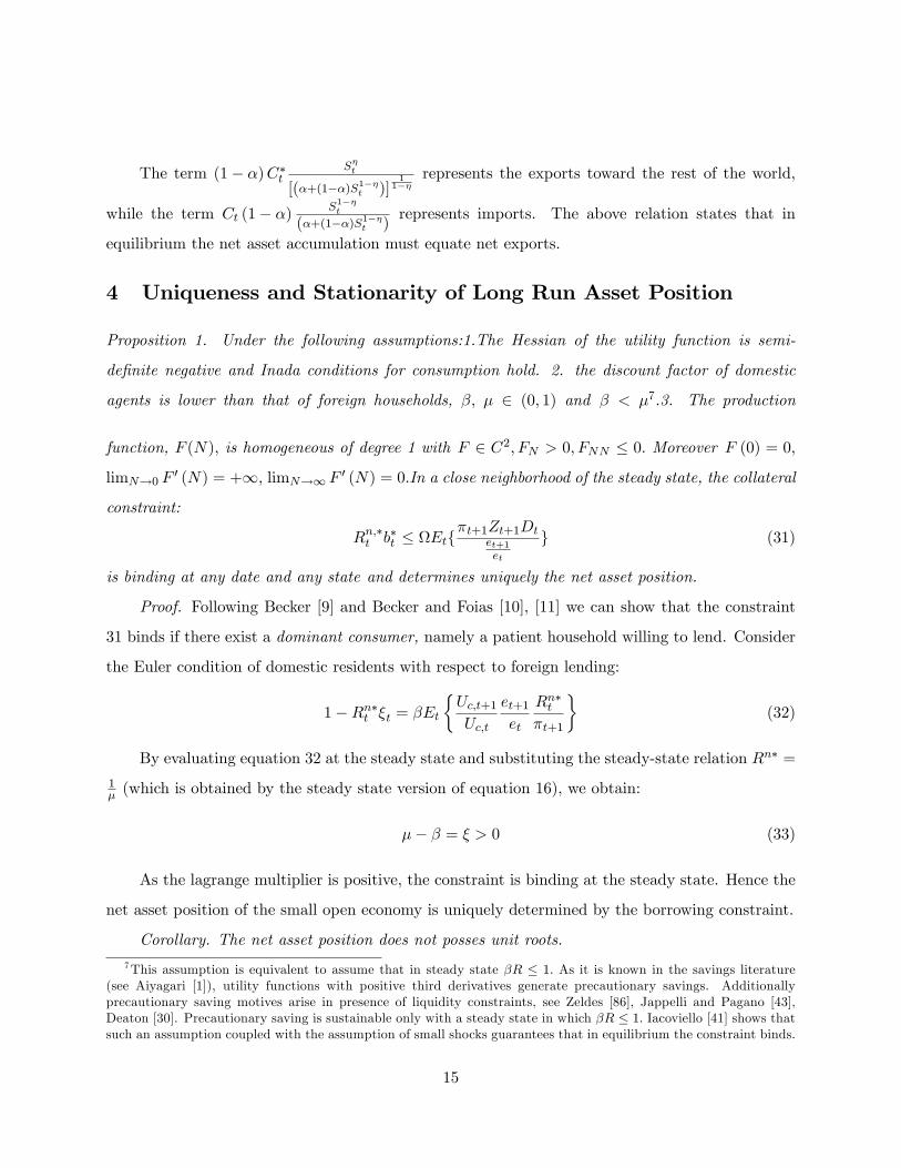
4 Uniqueness and Stationarity of Long Run Asset Position

Proposition 1. Under the following assumptions:1.The Hessian of the utility function is semi-

de�nite negative and Inada conditions for consumption hold. 2. the discount factor of domestic

agents is lower than that of foreign households, �; � 2 (0; 1) and � < �7:3. The production

function, F (N); is homogeneous of degree 1 with F 2 C2; FN > 0; FNN � 0: Moreover F (0) = 0;

limN!0 F0 (N) = +1; limN!1 F 0 (N) = 0:In a close neighborhood of the steady state, the collateral

constraint:

Rn;�t b�t � Etf�t+1Zt+1Dt

et+1et

g (31)

is binding at any date and any state and determines uniquely the net asset position.

Proof. Following Becker [9] and Becker and Foias [10], [11] we can show that the constraint

31 binds if there exist a dominant consumer, namely a patient household willing to lend. Consider

the Euler condition of domestic residents with respect to foreign lending:

1�Rn�t �t = �Et

�Uc;t+1Uc;t

et+1et

Rn�t�t+1

�(32)

By evaluating equation 32 at the steady state and substituting the steady-state relation Rn� =

1� (which is obtained by the steady state version of equation 16), we obtain:

�� � = � > 0 (33)

As the lagrange multiplier is positive, the constraint is binding at the steady state. Hence the

net asset position of the small open economy is uniquely determined by the borrowing constraint.

Corollary. The net asset position does not posses unit roots.

7This assumption is equivalent to assume that in steady state �R � 1: As it is known in the savings literature(see Aiyagari [1]), utility functions with positive third derivatives generate precautionary savings. Additionallyprecautionary saving motives arise in presence of liquidity constraints, see Zeldes [86], Jappelli and Pagano [43],Deaton [30]. Precautionary saving is sustainable only with a steady state in which �R � 1: Iacoviello [41] shows thatsuch an assumption coupled with the assumption of small shocks guarantees that in equilibrium the constraint binds.

15

As the Euler condition in the steady state, 33, does not depend on initial conditions but solely

on model parameters, the net asset position does not posses unit roots.

The above results move a step forward in understanding the conditions for stationarity of

the current account. In a seminal work, Obstfeld and Rogo¤ [66] have shown that under market

incompleteness the steady state of an open economy model is characterized by unit roots. This

implies that the steady state depends on initial values and transient shocks have long run e¤ects.

In previous works several methods have been proposed to recover stationarity: parameter and func-

tional form restrictions (see Cole and Obstfeld [26], Corsetti and Pesenti [27]), endogenous discount

factor (Uzawa-type preferences), debt-elastic interest-rate premium, convex portfolio adjustment

costs (see Schmitt-Grohe and Uribe [78]) or the assumption of �nitely lived agents (see Ghironi

[39]). Notice that imposing collateral constraints is iso-morphic to the introduction of debt elastic

interest rates, as the wedge, induced by the collateral constraint on the marginal rate of substitu-

tion between consumption at two di¤erent dates, behaves as a risk premium. However, while debt

elastic interest rates require an exogenously imposed long run level of external assets, collateral

constraints require �xing the debt to asset ratios, a value which can be more easily calibrated from

the data.

5 The Transmission of Shocks

Before turning to the evaluation of di¤erent exchange rate regimes and to the optimal policy design,

it is instructive to characterize the transmission mechanism in our model under �oating exchange

rates. We do that by looking at impulse response analysis under two shocks: productivity and

global liquidity shocks. We have chosen to consider a productivity shock as this is the main source

of business cycle �uctuations. We have chosen to consider a global liquidity shock as empirical

evidence has shown that this shock has had a signi�cant role in explaining house price movements

and in accounting for global imbalances8. Furthermore in a model with sticky prices, an interest

rate shock plays also the role of a demand shock.

8See for instance Sousa and Zaghini 2006, Rä¤er and Stracca 2006, Belke, Orth and Setzer 2008.

16

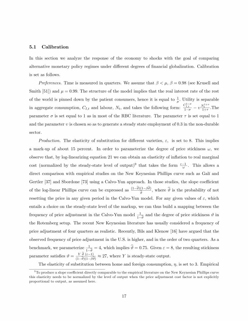
5.1 Calibration

In this section we analyze the response of the economy to shocks with the goal of comparing

alternative monetary policy regimes under di¤erent degrees of �nancial globalization. Calibration

is set as follows.

Preferences. Time is measured in quarters. We assume that � < �, � = 0:98 (see Krusell and

Smith [51]) and � = 0:99: The structure of the model implies that the real interest rate of the rest

of the world is pinned down by the patient consumers, hence it is equal to 1� : Utility is separable

in aggregate consumption, CI;t and labour, Nt; and takes the following form:C1��I;t

1�� � �N1+�t1+� :The

parameter � is set equal to 1 as in most of the RBC literature. The parameter � is set equal to 1

and the parameter � is chosen so as to generate a steady state employment of 0.3 in the non-durable

sector.

Production. The elasticity of substitution for di¤erent varieties, "; is set to 8. This implies

a mark-up of about 15 percent. In order to parameterize the degree of price stickiness !, we

observe that, by log-linearizing equation 21 we can obtain an elasticity of in�ation to real marginal

cost (normalized by the steady-state level of output)9 that takes the form "�1! . This allows a

direct comparison with empirical studies on the New Keynesian Phillips curve such as Galí and

Gertler [37] and Sbordone [73] using a Calvo-Yun approach. In those studies, the slope coe¢ cient

of the log-linear Phillips curve can be expressed as (1�b#)(1��b#)b# , where b# is the probability of notresetting the price in any given period in the Calvo-Yun model. For any given values of ", which

entails a choice on the steady-state level of the markup, we can thus build a mapping between the

frequency of price adjustment in the Calvo-Yun model 1

1�b# and the degree of price stickiness # inthe Rotemberg setup. The recent New Keynesian literature has usually considered a frequency of

price adjustment of four quarters as realistic. Recently, Bils and Klenow [16] have argued that the

observed frequency of price adjustment in the U.S. is higher, and in the order of two quarters. As a

benchmark, we parameterize 1

1�b# = 4, which implies b# = 0:75. Given " = 8, the resulting stickinessparameter satis�es # = Y b# ("�1)

(1�b#)(1��b#) � 27, where Y is steady-state output.

The elasticity of substitution between home and foreign consumption, �; is set to 3. Empirical

9To produce a slope coe¢ cient directly comparable to the empirical literature on the New Keynesian Phillips curvethis elasticity needs to be normalized by the level of output when the price adjustment cost factor is not explicitlyproportional to output, as assumed here.

17

studies assign values to this parameter that range from 2 to 5. The share of home consumption

goods in the domestic country, �; is set to 0:7; which implies, compatibly with empirical evidence

for industrialized countries, a degree of openness of 0.3:

Durables. The elasticity of substitution between durable and non-durable goods is set equal

to 1, while the share of durable spending is set to 0:2; a value consistent with industrialized

countries. Consistently with Erceg and Levin [33] the parameter in the adjustment cost function

is set to 300: This value allows to obtain a volatility for durable goods higher than the one for

non-durable, as suggested by empirical evidence. The quarterly depreciation rate of the durable

stock is set to � = 0:39764; this value is consistent with a speci�cation of the durable investment

which includes both consumer durables and residential investment: The baseline parameter that

de�nes the tightness of the endogenous borrowing limit is set consistently with loan to value ratios

for the industrialized countries over the period 1952-200510 which is 0.25. This parameter is varied

in the simulations in order to assess the role of �nancial globalization.

Stochastic processes. Following Prescott [71] and McCallum and Nelson [57] the standard

deviation of the productivity shock is set to 0:007 and its persistence is set to 0:95. Log-government

consumption evolves according to the following exogenous process, ln�gtg

�= �g ln

�gt�1g

�+ "gt ;

where the steady-state share of government consumption, g; is set so that gy = 0:25 and "gt is an

i.i.d. shock with standard deviation �g. Empirical evidence in Perotti [68] suggests �g = 0:008 and

�g = 0:9. We also introduce a global liquidity shock and interpret it as a shock to the aggregate

process of money supply in the rest of the world. As such we formalize it as an AR(1) shock to

foreign interest rate with �r = 0:00623 and �r = 0:6. Such calibration is consistent with estimates

of the interest rate process conducted by Rudebusch [76] and [77].

Monetary Policy regimes. There is an active monetary policy. The monetary authority sets

the short term nominal interest rate by reacting to endogenous variables as in the general class of

the Taylor rules:

Rnt = (�h;t��h)$�(

etet�1

)$e

1�$e (34)

where Rnt = RtPt+1Pt

; $� is the weight the monetary authority puts on the deviation of in�ation

from the target��;$e is the weight that the monetary authority puts on the deviation of the

10See IMF Report 2008.

18

exchange rate between two subsequent periods. We assign a value of 2 to the parameter $�: We

have chosen to target the change in the exchange rate, etet�1

; rather than the level, as this enlarges

the determinacy region as shown by Benigno, Benigno and Ghironi [13]. A regime of pure �oating

exchange rate is identi�ed by the case $e = 0: Pegged exchange rate regimes are identi�ed by a

Taylor rule of the form 34 in which $e > 0: This parameter will be varied in the simulations from

a low value of 0 to a high value of 0.911.

5.2 Dynamic Responses to Shocks

Figure 1 shows the dynamic response of selected variables to a 1% productivity shock in the

domestic economy. As it is standard in sticky prices models, output increases while in�ation

decreases. As technology has improved and since prices are sticky, �rms save on labour demand,

hence employment falls. The increase in output brings about an increase in non-durable and

durable consumption demand. The response of durables shows an hump-shaped dynamic due to

the presence of adjustment costs. The increase in durables is accompanied by a fall in its price.

Overall, however, the future value of durables (the value of collateral) increases. The increase in

the value of collateral allows to relax the borrowing constraint and to increase the supply of foreign

debt, as it is shown by the fact that the lagrange multiplier deviates from zero. As consumption

demand is higher than output, domestic residents increase their demand for foreign debt. In

equilibrium foreign lending increases. The ensuing current account de�cit induces a real exchange

rate depreciation. Notice that such movements of the current account are consistent with a couter-

cyclical net exports dynamic, a fact well established in international data. Importantly the current

account de�cit (which is the counterpart of the foreign debt accumulation) shows a persistent

dynamic. This is the sense in which our model can generate persistent global imbalances, despite

the long run stationarity featured by the current account dynamic.

Figure 2 shows impulse response of selected variables to 1% global liquidity shocks. Several

empirical studies have shown a link between housing demand (or durable demand) and the increase

in global liquidity. We therefore analyze the property of an increase in global liquidity, interpreted

a fall in foreign interest rate. The availability of foreign lending increases in this case. This

11 It is not possible to quantify this parameter empirically since the classi�cation between �oating and peggedexchange rate regimes is only done at a qualitative level. For this reason its value is varied in the experiments.

19

relaxes the borrowing constraint, therefore increasing the demand for both, durable and non-durable

consumption. Such an increase is accompanied by an increase in domestic prices, Ph;t; which renders

domestic goods less attractive. The ensuing switching expenditure e¤ect implies a fall in foreign

prices, Pf;t; and an exchange rate appreciation. Overall the CPI price index falls, as exports fall

by more than the increase in domestic demand. The fall in aggregate demand induces a fall in

employment and output. Hence while bene�cial on consumption demand such an ease in global

liquidity has a detrimental e¤ect on output.

6 Exchange Rate Regimes and Financial Globalization

We now turn to the evaluation of the stabilization properties of exchange rate pegs under di¤erent

degrees of �nancial globalization. A �rst step in this direction consists in analyzing the impact of

an increase in the degree of �nancial globalization for the dynamic of our economy. Recall that

we interpret �nancial globalization as an increase in the parameter : As debt in this economy

is denominated in foreign currency, exchange rate �uctuations will have an impact on the value

of collateral and through this on the dynamic of foreign debt and of other macro variables. The

higher is the degree of �nancial globalization, the higher is the destabilizing e¤ect that exchange

rate �uctuations have on foreign debt and the macro-economy. The combined e¤ect of �nancial

globalization and exchange rate �uctuations on foreign debt can be analyzed through the lenses of

the following two e¤ects:

1) Wedge/substitution e¤ect. Consider an expected exchange rate appreciation. A fall in the

exchange rate should increase the future value of collateral relative to the value of debt services,

as shown by the collateral constraint, Rn;�t b�t � tEtf�t+1Zt+1Dt

et+1et

g: As it stands clear from equation

13, when an additional unit of collateral becomes available the shadow value of relaxing the lia-

bility constraint, Uc;t�tEt

��t+1Zt+1

et+1et

�, changes. This shadow value represents an intertemporal

distortion in the value of durable consumption between two di¤erent dates. Such wedge behaves

as a tax on durable goods and changes in its magnitude can shift consumption from durable to

non-durable goods at the current date. An increase in the paramter has both a direct and an

indirect impact on this wedge. Those two e¤ects move actually in opposite directions. The direct

impact comes form the fact that the size of the wedge itself depends upon : A higher value of

20

this parameter increases credit availability therefore acting as a positive wealth shock that reduces

the demand for collateralizable durable goods. In other words an increase in increases the tax

on durable good, Uc;t�tEt

��t+1Zt+1

et+1et

�; as it reduces the marginal bene�t of durable relative to

non-durable at the current date. The indirect impact comes from the fact that a higher value of

; by relaxing the borrowing limit, reduces the size of �t. As the shadow value of the borrowing

limit decreases the marginal bene�t of one additional unit of collateral today increases. As �t enter

the durable tax component, a decrease in the lagrange multiplier will induce agents to substitute

non-durable with durable consumption goods. Quantitatively the �rst e¤ect seems to prevail, as,

while the sensitivity of non-durable consumption increases when increases, the contrary is true

for the demand in durable goods. The increase in consumption volatility feeds into output and

in�ation, therefore destabilizing the whole economy.

3) Valuation e¤ect. An exchange rate appreciation, by increasing the real value of collateral,

increases the borrowing capacity at the extensive margin. Such valuation e¤ect works in the same

direction as the wealth e¤ect, hence overall it tends to increase non-durable consumption volatility.

This in turn increases the volatility of output and in�ation as discussed previously.

Overall, it seems that increasing �nancial globalization tends to exacerbate the e¤ects of

exchange rate �uctuations and to destabilize the whole economy. Having established such link, the

policy maker in our economy faces a trade-o¤ in terms of in�ation versus exchange rate targeting.

On the one side, an exchange rate peg, accompanied to an increase in capital �ows, tends to

reduce the ability of the monetary authority to stabilize output and in�ation. Such an e¤ect,

�rst formalized in the Mundell-Fleming model, is known as the impossible trinity. On the other

side, higher �nancial globalization tends to exacerbate the destabilizing e¤ects of exchange rate

�uctuations on the whole economy and, because of this, calls for more aggressive exchange rate

target. In our model the second e¤ect tends to prevail as shown in Figure 9, 9 and 9. The three

�gures show the volatility (in percentage values) of output, in�ation and (non-durable) consumption

for di¤erent degrees of �nancial globalization and exchange rate target. To compute volatility we

consider all three shocks (productivity, government expenditure and foreign interest rate). The

�gures show that the volatility of the three variables considered increases whenever the degree

of �nancial globalization increases and decreases whenever the monetary authority increases the

21

weight on exchange rates. The monetary authority can minimize the volatility of all three variables

by applying an exchange rate target around 0.8.

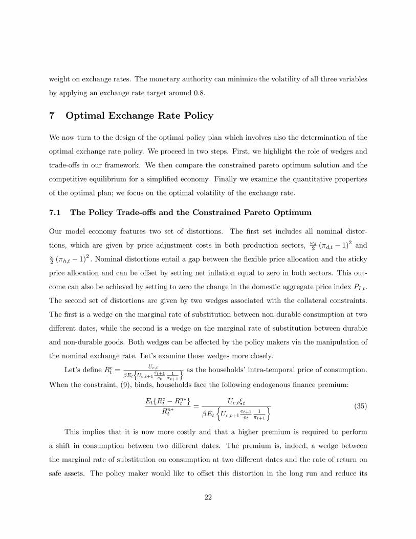
7 Optimal Exchange Rate Policy

We now turn to the design of the optimal policy plan which involves also the determination of the

optimal exchange rate policy. We proceed in two steps. First, we highlight the role of wedges and

trade-o¤s in our framework. We then compare the constrained pareto optimum solution and the

competitive equilibrium for a simpli�ed economy. Finally we examine the quantitative properties

of the optimal plan; we focus on the optimal volatility of the exchange rate.

7.1 The Policy Trade-o¤s and the Constrained Pareto Optimum

Our model economy features two set of distortions. The �rst set includes all nominal distor-

tions, which are given by price adjustment costs in both production sectors, !d2 (�d;t � 1)

2 and

!2 (�h;t � 1)

2 : Nominal distortions entail a gap between the �exible price allocation and the sticky

price allocation and can be o¤set by setting net in�ation equal to zero in both sectors. This out-

come can also be achieved by setting to zero the change in the domestic aggregate price index PI;t:

The second set of distortions are given by two wedges associated with the collateral constraints.

The �rst is a wedge on the marginal rate of substitution between non-durable consumption at two

di¤erent dates, while the second is a wedge on the marginal rate of substitution between durable

and non-durable goods. Both wedges can be a¤ected by the policy makers via the manipulation of

the nominal exchange rate. Let�s examine those wedges more closely.

Let�s de�ne Rct =Uc;t

�EtnUc;t+1

et+1et

1�t+1

o as the households�intra-temporal price of consumption.When the constraint, (9), binds, households face the following endogenous �nance premium:

EtfRct �Rn�t gRn�t

=Uc;t�t

�Et

nUc;t+1

et+1et

1�t+1

o (35)

This implies that it is now more costly and that a higher premium is required to perform

a shift in consumption between two di¤erent dates. The premium is, indeed, a wedge between

the marginal rate of substitution on consumption at two di¤erent dates and the rate of return on

safe assets. The policy maker would like to o¤set this distortion in the long run and reduce its

22

�uctuations in the short run. As �uctuations in the �nance premium are related to �uctuations

in the exchange rate and in the CPI in�ation rate, one way to achieve such a goal is to target

the exchange rate. Recall that also �uctuations in the CPI are linked to �uctuations in the real

exchange rate, as shown by equation 18.

The second wedge, induced by the presence of the collateral constraint, a¤ects the marginal

rate of substitution between durable and non-durable goods, as summarized by equation 13, and

is given by the following term:

Wedgec;d = Uc;t�tEt

(�t+1Zt+1

et+1et

)(36)

Notice that the size and the �uctuations of this wedge can be reduced by targeting the nominal

exchange rate alongside with the CPI. To summarize, both wedges can be o¤set by controlling

movements in the exchange rate.

Overall the policy maker would like to smooth �uctuations in foreign lending, as they reduce

the extent to which households can improve their consumption smoothing possibilities. As explained

before, �uctuations in foreign lending are jointly determined by equations 30 and 9. Both equations

highlight a clear link between �uctuations in external debt and the nominal exchange rate.

Generally speaking the policy maker is confronted with the following trade-o¤: on the one

side nominal rigidities require focusing on stabilization of domestic in�ation, with no attention to

�uctuations in the nominal exchange rate, on the other side, wedges associated with the presence

of collateral constraints, can be made inoperative by targeting the nominal exchange rate.

It is important to notice that the policy maker does not face any incentive to use exchange rate

�uctuations to render state contingent the collateral constraint. This would, indeed, be the case if

the foreign debt was limited by a constant: the policy maker could use �uctuations in the exchange

rate to ease the borrowing constraints in times of negative shocks. On the contrary, the collateral

constraint is state contingent by construction, hence the policy maker only faces an incentive to

smooth �uctuations in the value of external debt.

To highlight the role of the collateral constraint for the design of optimal monetary policy

it is instructive to derive the constrained pareto optimal allocation for the economy under �exible

prices. In this case all (gross) in�ation rates are set equal to one and the change in the nominal

23

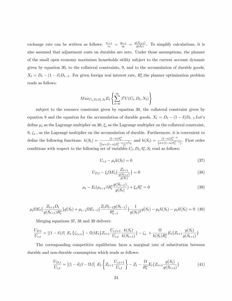
exchange rate can be written as follows: et+1et

= qt+1qt

= g(St+1)g(St)

. To simplify calculations, it is

also assumed that adjustment costs on durables are zero. Under those assumptions, the planner

of the small open economy maximizes households utility subject to the current account dynamic

given by equation 30, to the collateral constraints, 9, and to the accumulation of durable goods,

Xt = Dt � (1 � �)Dt�1. For given foreign real interest rate, R�t ;the planner optimization problem

reads as follows:

MaxCt;Dt;b�t ;StEt

( 1Xt=0

�tU(Ct; Dt; Nt)

)subject to the resource constraint given by equation 30, the collateral constraint given by

equation 9 and the equation for the accumulation of durable goods, Xt = Dt � (1 � �)Dt�1:Let�s

de�ne �t as the Lagrange multiplier on 30, �t as the Lagrange multiplier on the collateral constraint,

9, �t ; as the Lagrange multiplier on the accumulation of durable. Furthermore, it is convenient to

de�ne the following functions: h(St) =(1��)S�t

[(�+(1��)S1��t )]1

1��and k(St) =

(1��)S1��t

(�+(1��)S1��t ). First order

conditions with respect to the following set of variables Ct; Dt; b�t ; St read as follows:

Uc;t � �tk(St) = 0 (37)

UD;t � �tEtfZt+1g(St+1)g(St)

g = 0 (38)

�t � Et(�t+1�R�tg(St+1)

g(St)) + �tR

�t = 0 (39)

�tEtfZt+1Dt

g(St+1)R�tgg�(St) + �t�1Et�1f

ZtDt�1g(St�1)

R�t�1g 1

g(St)2g�(St)� �th�(St)� �tk�(St) = 0 (40)

Merging equations 37, 38 and 39 delivers:

UD;tUc;t

= [(1� �)�] Et��t+1

� �EtfZt+1

Uc;t+1Uc;t

k(St)

k(St+1)g � �t +

k(St)R�tEtfZt+1

g(St)

g(St+1)g

The corresponding competitive equilibrium faces a marginal rate of substitution between

durable and non-durable consumption which reads as follows:

UD;tUc;t

= [(1� �)� � �] Et�Zt+1

Uc;t+1Uc;t

�� Zt �

R�tEtfZt+1

g(St)

g(St+1)g (41)

24

Two considerations arise. First, one condition for the equivalence between the competitive

economy and the constraint pareto optimal allocation is obtained by setting, at each point in time,

the value of one unit of durable consumption, measured in utils, equal to the shadow value of

durable goods, namely �t = ZtUc;t. The comparison between the marginal rate of substitution

in the planner economy and the competitive economy sheds light on the planner behavior, who

internalizes the e¤ects that changes in the relative prices across countries have on the value of

collateral and on the marginal rate of substitution between durable and non-durable consumption.

7.2 Quantitative Properties of the Ramsey (Optimal) Monetary Policy

Given that higher �nancial globalization tends to exacerbate the destabilizing e¤ects of exchange

rate �uctuations, should the monetary authority optimally stabilize the exchange rate? In models

with sticky prices, the main distortion faced by the monetary authority is given by the cost of

in�ation �uctuations. Nominal frictions call for pure in�ation targeting, with no weight assigned to

either output �uctuations or to exchange rate �uctuations. This is the prescription advanced both

in closed12 and open economy model13. However in our model the planner faces a trade-o¤ between

stabilizing in�ation and stabilizing the exchange rate, as, in presence of high �nancial globalization,

the latter exacerbates ine¢ cient �uctuations in consumption. Hence the planner might want to

deviate from full price stability and trade-o¤s in�ation volatility with exchange rate stabilization.

We analyze the design of optimal monetary policy following the Ramsey approach14. The

optimal policy is determined by a monetary authority that maximizes the discounted sum of utilities

of all agents given the constraints of the competitive economy. The Lagrangian describing the

optimal plan can be constructed following two alternative approaches. The �rst is the primal

approach which amounts at describing the competitive equilibrium in terms of a minimal set of

relations involving only real allocations, in the spirit of the primal approach described in Lucas

and Stokey [55]. In the presence of sticky prices and borrowing constraints it is not possible to

reduce the planner�s problem to a maximization problem with a single implementability constraint.

12See Woodford [85], Clarida, Gali and Gertler [24] among others.13See for instance Obsteld and Rogo¤ [67], Benigno and Benigno [12], McCallum and Nelson [58], Corsetti and

Pesenti [28] and [28], Kollman [49], Devereux and Engel [31], Clarida, Galí, and Gertler [25], Galí and Monacelli [38].14See Ramsey [72], Atkinson and Stiglitz [3], Lucas and Stokey [55], Chari and Kehoe [?], Khan et al.[47], Schmitt-

Grohe and Uribe [74] among many others.

25

Hence we follow the alternative approach, which consists in maximizing agents�utility subject to

the full set of competitive economy equilibrium conditions and by keeping all prices. The optimal

policy plan for the domestic economy is determined by a monetary authority that maximizes the

discounted sum of utilities of all domestic residents:

Minf�nt g1t=0

Maxf�nt g1t=0

E0

( 1Xt=0

�tU(CI;t; Nt)

)(42)

given the constraints of the competitive economy represented by equations 5, 9, 10, 11, 12, 13, 16,

17, 18, 19, 21, 22, 24, 25, 26, 27.

As constraints 9, 11, 12, 13, 16, 21, 22, 27 exhibit future expectations of control variables, the

maximization problem of the Ramsey planner is intrinsically non-recursive. As �rst emphasized

in Kydland and Prescott [50], and then developed by Marcet and Marimon [56], a formal way to

rewrite the same problem in a recursive stationary form is to enlarge the planner�s state space with

additional (pseudo) co-state variables. Such variables bear the crucial meaning of tracking, along

the dynamics, the value to the planner of committing to the pre-announced policy plan.

The optimal monetary policy response to shocks is computed using second order approx-

imations15 of the �rst order conditions for the recursively stationary Lagrangian problem that

characterizes the Ramsey plan. Technically one needs to compute the stationary allocation that

characterizes the deterministic steady state of the �rst order conditions to the Ramsey plan. One

can then compute a second order approximation of the respective policy functions in the neighbor-

hood of the same steady state16. This amounts to implicitly assuming that the economy has been

15Second order approximation methods have the particular advantage of accounting for the e¤ects of volatility ofvariables on the mean levels. See among others, K. Judd, developed by C. Sims [80], S. Schmitt-Grohe and M. Uribe[79], F. Collard and M. Juillard [44].16Let�s assume that the system of Ramsey �rst order conditions takes the following form:

Etff(yt+1; yt; yt�1; ut; �)g = 0 (43)

where yt is the vector of endogenous variables (which includes both forward looking variables and pre-determined),ut is the vector of exogenous shocks, � is vector of parameters. Let�s further assume that the policy function takesthe following form:

yt = g(yt�1; ut; �)

The actual policy function can then be computed using the following approximation:

yt =�y + 0:5g���

2 + gy^y + guu+ 0:5(gyy(

^y ^

y)

+g uu(u u)) + gyu(^y u)

in which partial derivatives are obtained from the second order Taylor expansion of the system in 43.

26

evolving and policy has been conducted around such a steady already for a long period of time (in

a timeless perspective).

To analyze the trade-o¤ between in�ation and exchange rate stabilization the Ramsey plan is

simulated under the three shocks considered in order to compute the implied optimal volatility of

real exchange rate and in�ation.

Figure 9 shows results by plotting the optimal volatility (in percentage values) of real exchange

rate and of (annual) in�ation for di¤erent values of the degree of �nancial globalization. While

the volatility of the real exchange rate is largely stabilized for increasing values of the �nancial

openness, the volatility of in�ation is instead increasing signi�cantly. Hence, when the economy

becomes more �nancially globalized the trade-o¤ between in�ation and exchange rate stabilization

moves in favor of the latter. This is so since the wedges, induced by the presence of the collateral

constraints, become larger and more volatile, hence the policy maker faces a stronger incentive

to abate �uctuations in those wedges, a goal which is achieved by �ne tuning movements in the

exchange rates.

8 Conclusions

We have analyzed an economy in which consumption is �nanced through foreign lending. Net

lending toward the rest of the world is constrained by a borrowing limit motivated by limited

enforcement and borrowing is secured by collateral in the form of durable goods. We demonstrate

that although this economy can generate persistent current account de�cit it can still deliver a

stationary equilibrium. As �nancial globalization tends to exacerbate the destabilizing e¤ects of

exchange rate �uctuations, the monetary authority can achieve higher stabilization and welfare by

stabilizing the exchange rate. This implies that pure in�ation targeting strategies might not be

fully optimal for economies with large exposure to foreign debt and signi�cant global imbalances,

a condition which characterized several industrialized countries in the last decade.

27

9 Appendix 1. Net asset accumulation and current account

The market clearing condition for the non-durable sector in the small open economy reads as

follows:

Ah;tNh;t = �h��+ (1� �)S1��t

�i �1��

Ct + (1� �)�1

St

���C�t +

!

2(�h;t � 1)2 + gt (44)

After imposing the government budget constraint, the budget constraint of the borrowers in

the small open economy reads as follows:

Ct +Rn;�t�1

etet�1

b�t�1�t

+ Zt (Dt �Dt�1(1� �)) =Wt

PtNt + b

�t +

�h;tPt

+�d;tPt

� gt (45)

Let�s re-de�ne aggregate pro�ts as �h;t +�d;t = � which read as:

� = PtAh;tNh;t + Pd;tAd;tNd;t �WtNt � Pd;t!d2(�d;t � 1)2 � Ph;t

!

2(�h;t � 1)2

which in real terms becomes:

�

Pt=

�Ph;tPt

�Ah;tNh;t + ZtAd;tNd;t �

WtNt

Pt� Zt

!d2(�d;t � 1)2 �

�Ph;tPt

�!

2(�h;t � 1)2 + gt

Since Ah;tNh;t is given by equation 44 we obtain:

�

Pt=

�Ph;tPt

�"�h��+ (1� �)S1��t

�i �1��

Ct + (1� �)�1

St

���C�t +

!d2(�h;t � 1)2

#+ gt +

+ZtAd;tNd;t �WtNt

Pt� Zt

!d2(�d;t � 1)2 �

�Ph;tPt

�!

2(�h;t � 1)2

Moreover using the market clearing condition for the durable sector, as from equation 25, one

obtains:

�

Pt=

�Ph;tPt

�"�h��+ (1� �)S1��t

�i �1��

Ct + (1� �)�1

St

���C�t

#+ gt +

+Zt [Dt � (1� �)Dt�1]�WtNt

Pt

28

Substitute the latter expression into the households budget constraint leads to:

0 = Ct + Zt [Dt � (1� �)Dt�1] +Rn;�t�1

etet�1

b�t�1�t

� b�t �WtNt

Pt

�"�

Ph;tPt

�"���+ (1� �)S1��t

� �1��

Ct + (1� �)�1

St

���C�t

#+ Zt [Dt � (1� �)Dt�1]�

WtNt

Pt

#

Finally after some manipulation and using the expression for the price index, Pt = Ph;t

h��+ (1� �)S1��t

�i 11��

leads to:

Rn;�t�1etet�1

b�t�1�t

� b�t = (1� �)C�tS�th�

�+ (1� �)S1��t

�i 11��

� Ct (1� �)S1��t�

�+ (1� �)S1��t

�which states that the �ow of external debt must equate net exports.

.

29

References

[1] Aiyagari, S. Rao (1994). �Uninsured idiosyncratic risk, and aggregate saving.�Quarterly Jour-

nal of Economics, 109, 659�684.

[2] Aoki, Kosuke, Gianluca, Benigno and Nobu Kiyotaki, (2005). �Adjusting to Capital Liberal-

ization�. Mimeo.

[3] Atkinson, Anthony B. and Joseph Stiglitz, (1976). �The Design of Tax Structure: Direct Versus

Indirect Taxation�, Journal of Public Economics, 6, 1-2, 55-75.

[4] Attanasio, Orazio P. , Goldberg, Pinelopi K. and Ekaterini Kyriazidou (2008). �Credit Con-

straints in the Market for Consumer Durables: Evidence from Micro Data on Car Loans�.

International Economic Review, 401-36.

[5] Backus, David, Espen Henricksen, Frederic Lambert and Chris Telmer, (2005). �Current Ac-

count Fact and Fiction�. Mimeo.

[6] Backus, David and Patrick, Kehoe, (1989). �International Evidence on the Historical Prop-

erties of the Business Cycles�. W.p. 402R, Federal Reserve Bank of Minneapolis, Research

Department.

[7] Backus, David K., Kehoe Patrick J. and Kydland, Finn E. (1992). �International Real Business

Cycles�. Journal of Political Economy, 101, 745-775.

[8] Barsky, Robert, Christopher House and Miles Kimball, (2005). �Sticky Price Models and

Durable Goods�. American Economic Review, 97(3), 984-998.

[9] Becker, Robert A, (1980). �On the Long-Run Steady State in a Simple Dynamic Model of

Equilibrium with Heterogeneous Households.�Quarterly Journal of Economics, 95 (2), 1980,

375 - 382.

[10] Becker, Robert A. and Foias, Ciprian, (1987). �A characterization of Ramsey equilibrium�.

Journal of Economic Theory, vol. 41(1), 173-184.

30

[11] Becker, Robert A. and Foias, Ciprian, (1994). �The Local Bifurcation of Ramsey Equilibrium.�

Economic Theory, vol. 4(5), 719-44.

[12] Benigno, Pierpaolo and Gianluca Benigno, (2003). �Price Stability Open Economies�, Review

of Economic Studies, 60,4.

[13] Benigno, Gianluca, Benigno Pierpaolo and Fabio Ghironi, (2007). �Interest Rate Rules for

Fixed Exchange Rate Regimes.� Journal of Economic Dynamics and Control, 31(7), 2196-

2211.

[14] Benigno, Gianluca, Huigang Chen, Christopher Otrok, Alessandro Rebucci, Eric Young,

(2010). �Revisiting Overborrowing and Its Policy Implications�. Mimeo.

[15] Bernanke, Ben, (2005). �The global saving glut and the US current account de�cit�. The

Federal Reserve Board.

[16] Bils M. and P. Klenow, (2004). �Some Evidence on the Importance of Sticky Prices.�Journal

of Political Economy, October.

[17] Black, J.M., de Meza, D., Je¤reys, D., (1996). �House prices, the supply of collateral and the

enterprise economy.�Economic Journal.

[18] Broner, Fernando and Ventura, Jaume, (2008). �Rethinking the e¤ects of �nancial liberaliza-

tion.�Economics Working Papers 1128, Department of Economics and Business, Universitat

Pompeu Fabra.

[19] Campbell, Je¤rey Y. and Zvi Hercowitz, (2006). �The Role of Collateralized Household Debt

in Macroeconomic Stabilization�. NBER w.p. 11330.

[20] Carlstrom, Charles and Timothy Fuerst, (2006). �Co-movement in Sticky Price Models with

Durable Goods�. Mimeo.

[21] Chang, Robert, Cespedes, Luis and Andre Velasco, (2004). �Balance Sheets and Exchange

Rate Policy�, American Economic Review.

31

[22] Chari, Varadarajan V. and Patrick J. Kehoe, (1999). �Optimal Fiscal and Monetary Policy�,

in Handbook of Macroeconomics, M. Woodford and J. Taylor Eds., North Holland.

[23] Chari, V.V., Kehoe, Patrick J. and McGrattan, Ellen R., (2005). �Sudden Stops and Output

Drops�. American Economic Review Papers and Proceedings.

[24] Clarida, Richard, Jordi Gali, and Mark Gertler, (2000). Monetary Policy Rules and Macro-

economic Stability: Evidence and Some Theory. Quarterly Journal of Economics, 115 (1),

147-180.

[25] Clarida, Richard, Jordi Galí, and Mark Gertler (2002). �A Simple Framework for International

Monetary Policy Analysis.�Journal of Monetary Economics, vol. 49, no. 5, 879-904.

[26] Cole, Harald and Maurice Obstfeld, (1989). �Commodity Trade and International Risk Shar-

ing: How Much Do Financial Markets Matter�. Journal of Monetary Economics, 28(1), 3-24.

[27] Corsetti, Giancarlo and Paolo Pesenti, (2001). �Welfare and Macroeconomic Interdependence�.

Quarterly Journal of Economics.

[28] Corsetti, Giancarlo and Paolo Pesenti, (2003). �International Dimensions of Optimal Monetary

Policy�, Journal of Monetary Economics.

[29] Davis, Morris and Jonathan, Heatcote, (2005). �Housing and the Business Cycle�. Interna-

tional Economic Review, 46(3), 751-784.

[30] Deaton, Angus, (1991). �Saving and Liquidity Constraints�. Econometrica, 59, 1221-1248.

[31] Devereux, Michael B. and Charles Engel, (2003). �Monetary Policy in the Open Economy Re-

visited: Exchange Rate Flexibility and Price Setting Behavior,�Review of Economic Studies,

60, 765-783.

[32] Devereux, Michael B. and Alan Sutherland, (2007). �Monetary Policy and Portfolio Choice in

an Open Economy Macro Model.�Journal of the European Economic Association, MIT Press,

vol. 5(2-3), pages 491-499, 04-05.

32

[33] Erceg, Chris and Andrew Levin, (2005). �Optimal Monetary Policy with Durable Consumption

Goods�. International �nance Discussion Paper 748, Board of Governors.

[34] Faia, Ester (2007), �Finance and International Business Cycles�, Journal of Monetary Eco-

nomics.

[35] Faia, Ester and Tommaso, Monacelli, (2008). �Optimal Monetary Policy in A Small Open

Economy with Home Bias�. Journal of Money, Credit and Banking,vol. 40, pages 721-750.

[36] Friedman, Milton, (1959). �The Optimum Quantity of Money�, in The Optimum Quantity of

Money, and Other Essays, Aldine Publishing Company, Chicago.

[37] Galí, Jordi and Mark Gertler, (1999).�In�ation Dynamics: A Structural Econometric Analy-

sis�. Journal of Monetary Economics, vol. 44, no 2, 195-222.

[38] Galí, Jordi and Tommaso Monacelli, (2005). �Monetary Policy and Exchange Rate Volatility

in a Small Open Economy�, Review of Economic Studies, vol. 72, issue 3, 2005, 707-734.

[39] Ghironi, Fabio, (2008). �The Role of Net Foreign Assets in a New Keynesian Small Open

Economy Model�. Journal of Economic Dynamics and Control (forthcoming).

[40] Gertler M., Gilchrist S. and F.M. Natalucci, (2007). �External Constraints on Monetary Policy

and The Financial Accelerator�, Journal of Money, Credit and Banking

[41] Iacoviello, Matteo, (2005). �House Prices, Borrowing Constraints and Monetary Policy in the

Business Cycle�. American Economic Review, 95(3), 739-764.

[42] Iacoviello, Matteo, and Raoul Minetti, (2006) �International Business Cycles with Domestic

and Foreign Lenders�. Journal of Monetary Economics, 53 (8), 2267-2282.

[43] Jappelli, Tullio and Marco Pagano, (1994). �Saving Growth and Liquidity Constraints�. Quar-

terly Journal of Economics, 109, 83-109.

[44] Juilliard, Michel and Fabrice, Collard (2001). �A Higher-Order Taylor Expansion Approach to

Simulation of Stochastic Forward-Looking Models with an Application to a Nonlinear Phillips

Curve Model�. Computational Economics, vol. 17, pp. 125-139.

33

[45] Judd, Kenneth, (1998). Numerical Methods in Economics, Cambridge, MA, MIT Press.

[46] Kiyotaki, Nobuhiro and Moore, John. (1997) �Credit Cycle�. Journal of Political Economy,

105(2), pp. 211-48.

[47] Khan, Aubhik, Robert King and Alexander L. Wolman, (2003). �Optimal Monetary Policy�,

Review of Economic Studies, 60,4.

[48] Kocherlacota, Narayana, (2000). �Creating Business Cycles Through Credit Constraints�. Fed-

eral Reserve Bank of Minneapolis Quarterly Review, 24(3), 2-10.

[49] Kollmann, Robert, (2001). �The Exchange Rate in a Dynamic Optimizing Current Account

Model with Nominal Rigidities: A Quantitative Investigation,�Journal of International Eco-

nomics vol.55, 243-262.

[50] Kydland, Finn and Edward C. Prescott, (1980). �Dynamic Optimal Taxation, Rational Ex-

pectations and Optimal Control�. Journal of Economic Dynamics and Control 2:79-91.

[51] Krusell, Per and A. Smith, (1998). �Income and Wealth Heterogeneity in the Macroeconomy�.

Journal of Political Economy, 106, 867-896.

[52] Lahiri, A. R., R. Singh and Carlos Vegh, (2007). �Segmented Asset Markets and Optimal

Exchange Rate Regimes�, Journal of International Economics 72, 1-21.

[53] Lane, Philip, GianMaria Milesi-Ferretti, (2001). �The External Wealth of Nations: Estimates

of Foreign Assets and Liabilities for Industrial and Developing Countries�. Journal of Inter-

national Economics, 55, 263-94.

[54] Levchenko, Andrei, (2005). �Financial Liberalization and Consumption Volatility in Develop-

ing Countries�. IMF Sta¤ Papers 52, 2.

[55] Lucas, Robert E. and Nancy Stokey, (1983). �Optimal Fiscal and Monetary Policy in an

Economy Without Capital�, Journal of Monetary Economics, 12:55-93.

[56] Marcet, Albert and Ramon Marimon, (1999). Recursive Contracts. Mimeo, Universitat Pom-

peu Fabra and European University Institute.

34

[57] McCallum, Bennett and Edward Nelson, (2000). �An Optimizing IS-LM Speci�cation for

Monetary Policy and Business Cycle Analysis�. Journal of Money, Credit and Banking, 31(3),

296-316.

[58] McCallum, Bennett and Edward Nelson, (2000). �Monetary Policy for an Open Economy:

An Alternative Framework with Optimizing Agents and Sticky Prices�, Oxford Review of

Economic Policy 16, 74-91.

[59] Mendoza, Enrique G., (1991). �Real Business Cycle in a Small Open Economy�. American

Economic Review, 81(4), 797-818.

[60] Mendoza, Enrique, (2006). �Endogenous Sudden Stops in a Business Cycle Model with Col-

lateral Constraints: A Fisherian De�ation of Tobin�s Q�. Manuscript, University of Maryland.

[61] Mendoza, Enrique, and Katherine, Smith, (2006). �Quantitative Implications of a Debt De-

�ation Theory of Sudden Stops and Asset Prices�. Forthcoming Journal of International Eco-

nomics.

[62] Mendoza, Enrique, Vincenzo Quadrini and Viktor Rios-Rull, (2007). �On the Welfare Impli-

cations of Financial Globalization without Financial Development�. International Seminar on

Macroeconomics.

[63] Mendoza, Enrique, Vincenzo Quadrini and Viktor Rios-Rull, (2009). �Financial Integration,

Financial Deepness and Global Imbalances.�Journal of Political Economy, 117(3).

[64] Miles, David, (1992). �Housing Markets, Consumption and Financial Liberalization in Major

Economies�. European Economic Review, 36, 1093-1127.

[65] Monacelli, Tommaso, (2009). �New Keynesian models, durable goods, and collateral con-

straints�. Journal of Monetary Economics, Volume 56, Issue 2, Pages 137-282.

[66] Obstfeld, Maurice, and Kenneth Rogo¤, (1995). �Exchange Rate Dynamics Redux�. Journal

of Political Economy, 103, 624-60.

35

[67] Obstfeld Maurice and Kenneth Rogo¤, (2000). �The Six Major Puzzles in International Macro-

economics: Is There a Common Cause?�. Macroeconomics Annual, B. Bernanke and K. Rogo¤

eds.

[68] Perotti, Roberto, (2004). �Estimating the E¤ects of Fiscal Policy in OECD Countries�. Mimeo.

[69] Perri, Fabrizio and Vincenzo Quadrini. (2008) �Understanding the International Great Mod-

eration�. Manuscript.

[70] Perri, Fabrizio, (2007). �Default and Enforcement Constraints�. The New Palgrave Dictionary

in Economics.

[71] Prescott, Edward, (1986). �Theory Ahead of Business Cycle Measurement�. Carnegie

Rochester Series on Public Policy, 24:11-44.

[72] Ramsey, Frank P., (1927). �A contribution to the Theory of Taxation�. Economic Journal,

37:47-61.

[73] Sbordone, Argia (2002). �Prices and Unit Labor Costs: A New Test of Price Stickiness�.

Journal of Monetary Economics Vol. 49 (2).

[74] Schmitt-Grohe, Stephanie and Martin Uribe (2004). �Optimal Fiscal and Monetary Policy

under Sticky Prices�, Journal of Economic Theory, 114,198-230.

[75] Rotemberg, Julio, (1982). �Monopolistic Price Adjustment and Aggregate Output�. Review of

Economics Studies, 44, 517-531.

[76] Rudebusch, Glenn (2002). �Term Structure Evidence on Interest Rate Smoothing and Mone-

tary Policy Inertia.�Journal of Monetary Economics, Vol. 49, pp. 1161-1187.

[77] Rudebusch, Glenn (2006). �Monetary Policy Inertia: Fact or Fiction?� International Journal

of Central Banking, Vol. 2, No. 3, pp. 85-135.

[78] Schmitt-Grohe, Stephanie and Uribe, Martin, (2003). �Closing Small Open Economy Models�.

Journal of International Economics, 61, 163-185.

36

[79] Schmitt-Grohe, S., Uribe, M. (2004a). � Solving Dynamic General Equilibrium Models Using

a Second-Order Approximation to the Policy Function�. Journal of Economic Dynamics and

Control 28, 645-858.

[80] Sims, Christopher, �Second Order Accurate Solution of Discrete Time Dynamic Equilibrium

Models.�Manuscript. Princeton: Princeton University,

[81] December 2000b.

[82] Sutherland, Alan, (2002). �International Monetary Policy Coordination and Financial Market

Integration�CEPR Discussion Paper No 4251.

[83] Topel, Robert and Sherwin Rosen, (1988). �Housing Investment in the United States�. Journal

of Political Economy, 96(4).

[84] Uribe, Martin. (2006) �On Overborrowing�. American Economic Review Papers and Proceed-

ings, 86, 417-421.

[85] Woodford, Michael (2003). Interest and Prices. Princeton University Press.

[86] Zeldes, Stephen, (1989). �Consumption and Liquidity Constraints�. Journal of Political Econ-

omy, 97, 305-346.

37

0 5 1 0 1 5 2 0 2 5 3 0 3 5 4 0 4 5 5 00 .2

0 .4

0 .6

0 .8

1

tim e

% d

evia

tion

 from

 s.s

O u tp u t

0 5 1 0 1 5 2 0 2 5 3 0 3 5 4 0 4 5 5 0­ 0 .5

0

0 .5

1

tim e

% d

evia

tion

 from

 s.s

I n f latio n  ( an n u al)

0 5 1 0 1 5 2 0 2 5 3 0 3 5 4 0 4 5 5 00

0 .5

1

1 .5

tim e

% d

evia

tion

 from

 s.s

Co n su m p tio n

0 5 1 0 1 5 2 0 2 5 3 0 3 5 4 0 4 5 5 0­ 0 .2

­ 0 .1 5

­ 0 .1

­ 0 .0 5

0

tim e

% d

evia

tion

 from

 s.s

Em p lo y m en t

0 5 1 0 1 5 2 0 2 5 3 0 3 5 4 0 4 5 5 0­ 0 .5

0

0 .5

1

1 .5

tim e

% d

evia

tion

 from

 s.s

L ag r an g e m u ltip lier

0 5 1 0 1 5 2 0 2 5 3 0 3 5 4 0 4 5 5 00

0 .0 2

0 .0 4

0 .0 6

tim e

% d

evia

tion

 from

 s.s

D u r ab les  ( s to ck )

0 5 1 0 1 5 2 0 2 5 3 0 3 5 4 0 4 5 5 0­ 0 .2

0

0 .2

0 .4

0 .6

tim e

% d

evia

tion

 from

 s.s

F o r eig n  d eb t

0 5 1 0 1 5 2 0 2 5 3 0 3 5 4 0 4 5 5 00

0 .1

0 .2

0 .3

0 .4

tim e

% d

evia

tion

 from

 s.s

Real ex ch an g e r ate

Figure 1: Impulse responses to domestic productivity shock

38

0 5 1 0 1 5 2 0 2 5 3 0­ 0 .3

­ 0 .2

­ 0 .1

0

0 .1

tim e

% d

evia

tion

 from

 s.s

O u tp u t

0 5 1 0 1 5 2 0 2 5 3 0­ 1

­ 0 .5

0

0 .5

tim e

% d

evia

tion

 from

 s.s

I n f latio n  ( an n u al)

0 5 1 0 1 5 2 0 2 5 3 0­ 0 .2

0

0 .2

0 .4

0 .6

tim e

% d

evia

tion

 from

 s.s

Co n su m p tio n

0 5 1 0 1 5 2 0 2 5 3 0­ 0 .2

­ 0 .1

0

0 .1

0 .2

tim e

% d

evia

tion

 from

 s.s

Em p lo y m en t

0 5 1 0 1 5 2 0 2 5 3 00

2

4

6

tim e

% d

evia

tion

 from

 s.s

Lag r an g e m u ltip lier

0 5 1 0 1 5 2 0 2 5 3 00

2

4

6x  1 0

­3

tim e

% d

evia

tion

 from

 s.s

D u r ab les ( s to ck )

0 5 1 0 1 5 2 0 2 5 3 00

0 .2

0 .4

0 .6

0 .8

tim e

% d

evia

tion

 from

 s.s

F o r eig n  d eb t

0 5 1 0 1 5 2 0 2 5 3 0­ 0 .4

­ 0 .3

­ 0 .2

­ 0 .1

0

tim e

% d

evia

tion

 from

 s.s

Real ex ch an g e r ate

Figure 2: Impulse responses to global liquidity shock (a fall in foreign interest rates).

39

00.1

0.20.3

0.40.5

0.60.7

0.80.9

0

0.1

0.2

0.3

0.4

0.5

0.6

0.7

0.8

0.90.0182

0.0184

0.0186

0.0188

0.019

0.0192

0.0194

Exchange rate target in monetary policy rule

Figure 3: Volatitlity of output for different degrees of financial globalization and exchange rate target

Degree of financial globalization

40

00.1

0.20.3

0.40.5

0.60.7

0.80.9

0

0.1

0.2

0.3

0.4

0.5

0.6

0.7

0.8

0.90.0258

0.026

0.0262

0.0264

0.0266

0.0268

0.027

0.0272

0.0274

0.0276

Exchange rate target in monetary policy rule

Figure 4: volatility of consumption for different degrees of financial globalization and exchange rate target

Degree of financial globalization

41

00.1

0.20.3

0.40.5

0.60.7

0.80.9

0

0.1

0.2

0.3

0.4

0.5

0.6

0.7

0.8

0.90.5

1

1.5

2

2.5

3

3.5

4

4.5

5

5.5

x 10 ­3

Exchange rate target in monetary policy rule

Figure 5:volatitlity of CPI inflation for different degrees of exchange rate target and financial globalization

Degree of financial globalization

42

0 0.1 0.2 0.3 0.4 0.5 0.6 0.7 0.8 0.90.028

0.029

0.03

0.031

0.032

0.033

0.034

0.035

0.036

0.037

Degree of financial globalization

Vol

atili

ty (%

 val

ues)

real exchange rateAnnual inflation

43