Embed Size (px)
Citation preview
NBER WORKING PAPER SERIES
FINANCIAL FLOWS AND THE INTERNATIONAL MONETARY SYSTEM
Evgenia PassariHélène Rey
Working Paper 21172http://www.nber.org/papers/w21172
NATIONAL BUREAU OF ECONOMIC RESEARCH1050 Massachusetts Avenue
Cambridge, MA 02138May 2015
Sargan Lecture, Royal Economic Society (2014). Rey gratefully acknowledges financial support fromthe European Research Council (Grant 210584). We thank the editor Morten Ravn for comments.We are very grateful to Elena Gerko, Silvia Miranda Agrippino, Nicolas Coeurdacier, Pablo Winant,Xinyuan Li, Richard Portes and Jay Shambaugh for discussions. We also heartfully thank Peter Karadiand Mark Gertler for sharing their instruments. The views expressed herein are those of the authorsand do not necessarily reflect the views of the National Bureau of Economic Research.
NBER working papers are circulated for discussion and comment purposes. They have not been peer-reviewed or been subject to the review by the NBER Board of Directors that accompanies officialNBER publications.
© 2015 by Evgenia Passari and Hélène Rey. All rights reserved. Short sections of text, not to exceedtwo paragraphs, may be quoted without explicit permission provided that full credit, including © notice,is given to the source.
Financial Flows and the International Monetary SystemEvgenia Passari and Hélène ReyNBER Working Paper No. 21172May 2015JEL No. E5,F3
ABSTRACT
We review the findings of the literature on the benefits of international financial flows and find thatthey are quantitatively elusive. We then present evidence on the existence of a global cycle in grosscross border flows, asset prices and leverage and discuss its impact on monetary policy autonomyacross different exchange rate regimes. We focus in particular on the effect of US monetary policyshocks on the UK's financial conditions.
Evgenia PassariUniversite Paris [email protected]
Hélène ReyLondon Business SchoolRegents ParkLondon NW1 4SAUNITED KINGDOMand [email protected]
Keynes in the ’Economic consequences of peace’ published in 1920 lauded thebenefits of international integration in trade and financial flows. He explainedhow before the first world war,
...the inhabitant of London could order by telephone, sipping hismorning tea in bed, the various products of the whole earth, insuch quantity as he might see fit, and reasonably expect their earlydelivery upon his doorstep; he could at the same moment and by thesame means adventure his wealth in the natural resources and newenterprises of any quarter of the world, and share, without exertionor even trouble, in their prospective fruits and advantages; or hecould decide to couple the security of his fortunes with the good faithof the townspeople of any substantial municipality in any continentthat fancy or information might recommend.
(Keynes, 1920, p.11)
After some important setbacks during the wars and the Great Depression,financial openness seems to have resumed its long run upward trajectory. Bothemerging markets and advanced economies are increasingly holding large amountsof assets cross border, even though the 2007 crisis has moderated the trend. Asimple and widely used measure of de facto financial integration, the sum ofcross-border financial claims and liabilities, scaled by annual GDP has risenfrom about 70% in 1980 to 440% in 2007 for advanced economies, and fromabout 35% to 70% for emerging markets during the same period (see Lane(2012)). The gross external assets and liabilities of the UK were 488% and507% of annual output respectively in 2010.1
The menu of assets exchanged across borders has also become broader withderivatives and asset backed mortgage securities becoming internationally traded.It is increasingly important to look at the entire external balance sheet of coun-tries (and not only at net positions) to understand the financial strength andvulnerabilities of countries. As discussed in Gourinchas and Rey (2014), the ex-ternal assets of the United States for example are tilted towards “risky assets”,equity and FDI which constitute about 49% of total assets between 1970 and2010, while external US liabilities consist mostly of “safer assets” such as debtand bank credit. Such heterogeneity in the composition of the balance sheetsopens the door to large valuation effects and potentially large wealth transfersacross countries (see Gourinchas and Rey 2007 and Gourinchas, Rey and Truem-pler (2012) who estimate valuation changes during the 2008 crisis). Gourinchas,Rey and Govillot (2010) provide a theoretical model of these transfers and showthat the US plays the role of the world insurer during global crises.
The scope for international capital flows to provide welfare gains or losseshas therefore increased considerably in recent decades. The academic literaturehas attempted to measure gains to financial integration mainly in two ways:
1Lane and Milesi Ferretti (2007) updated. We report external assets and liabilities exclud-ing financial derivatives.
1
by testing for growth effects and better risk sharing following financial accountopening using either panel data or event studies and by calibrating standardinternational macroeconomic models and computing gains when going from au-tarky to financially integrated markets. Perhaps surprisingly, both streams ofliterature have so far failed to deliver clear cut results supporting large gains tofinancial integration. In the international risk sharing literature, there is stilla lively debate regarding the gains that can be achieved by diversification ofthe portfolios (Obstfeld (2009), Van Wincoop (1994,1999), Lewis (1999, 2000),Coeurdacier and Rey (2013), Lewis and Liu(2014)). In the allocative efficiencyliterature based on the neoclassical growth model, gains have been found to berelatively small (Gourinchas and Jeanne (2006) and Coeurdacier et al. (2014))though Hoxha et al. (2013) find larger gains if capital goods are imperfect sub-stitutes. Recent surveys of the empirical literature such as Jeanne et al. (2012)tend to conclude that there is little support in the data for large gains fromfinancial integration.
On the other hand, some costs to integration, due in particular to mone-tary policy spillovers have become more apparent with the recent crisis. Theinternational finance literature has often used the framework of the Mundel-lian “trilemma”: in a financially integrated world, fixed exchange rates exportthe monetary policy of the base country to the periphery. The corollary isthat if there are free capital flows, it is possible to have independent monetarypolicies only by having the exchange rate float; and conversely, that floatingexchange rates enable monetary policy independence (see e.g. Obstfeld andTaylor (2004)). But does the current scale of financial integration put even thisinto question? Are the monetary conditions of the main world financing cen-tres, in particular the United States, setting the tone globally, regardless of theexchange-rate regime of countries?
In the second section of the paper we discuss the sources of potential gainsfrom financial integration and will assess their magnitude in the context of thetextbook neoclassical growth model. In the third part, we discuss the costs offinancial integration in the form of loss of monetary policy autonomy. We showthe existence of a global financial cycle and discuss its characteristics. In a fourthpart, we then investigate in more details whether the exchange rate regime altersthe transmission of financing conditions and monetary policy shocks. In the lastpart we analyse the effect of US monetary policy on the global financial cycleand explore empirically whether a flexible exchange rate regime (the one of theUnited Kingdom) insulates countries from US monetary policy shocks.
1 Welfare benefits of financial capital flows
The welfare benefits of financial integration is one of the long standing issuesin international finance. The neoclassical growth model is behind many of oureconomic intuitions regarding why the free flow of capital could be beneficial.Within this model, financial integration brings improvements in allocative effi-ciency as capital flows to places with the highest marginal product, i.e. capital
2
scarce economies. As explained in Gourinchas and Rey (2014),2 those countriesare characterised with a high autarky rate of interest compared to the worldinterest rate. Emerging markets, which tend to be more capital scarce thanmature OECD economies, should hence benefit from financial integration asimported capital enables them to consume and invest at a faster pace than ifthey had remained in financial autarky.
It is only recently (see Gourinchas and Jeanne (2006)) that the welfare gainsof going from autarky to a world where a riskless bond can be traded interna-tionally have been evaluated quantitatively in the textbook deterministic neo-classical growth model with one good. Interestingly, those welfare gains havebeen found to be small: they are worth a few tenths of a % of permanent con-sumption for a small open economy even if it starts with a relatively high levelof capital scarcity (calibrated to match the actual capital scarcity of emerg-ing markets). The reason is that financial integration enables an economy tospeed up its transition towards its steady-state capital stock but that does notbring large welfare gains as the distortion induced by a lack of capital mobilityis transitory: the country would have reached its steady-state level of capitalregardless of financial openness, albeit at a slower speed. In this framework,only very capital-scarce countries could possibly experience significant gains tofinancial integration.
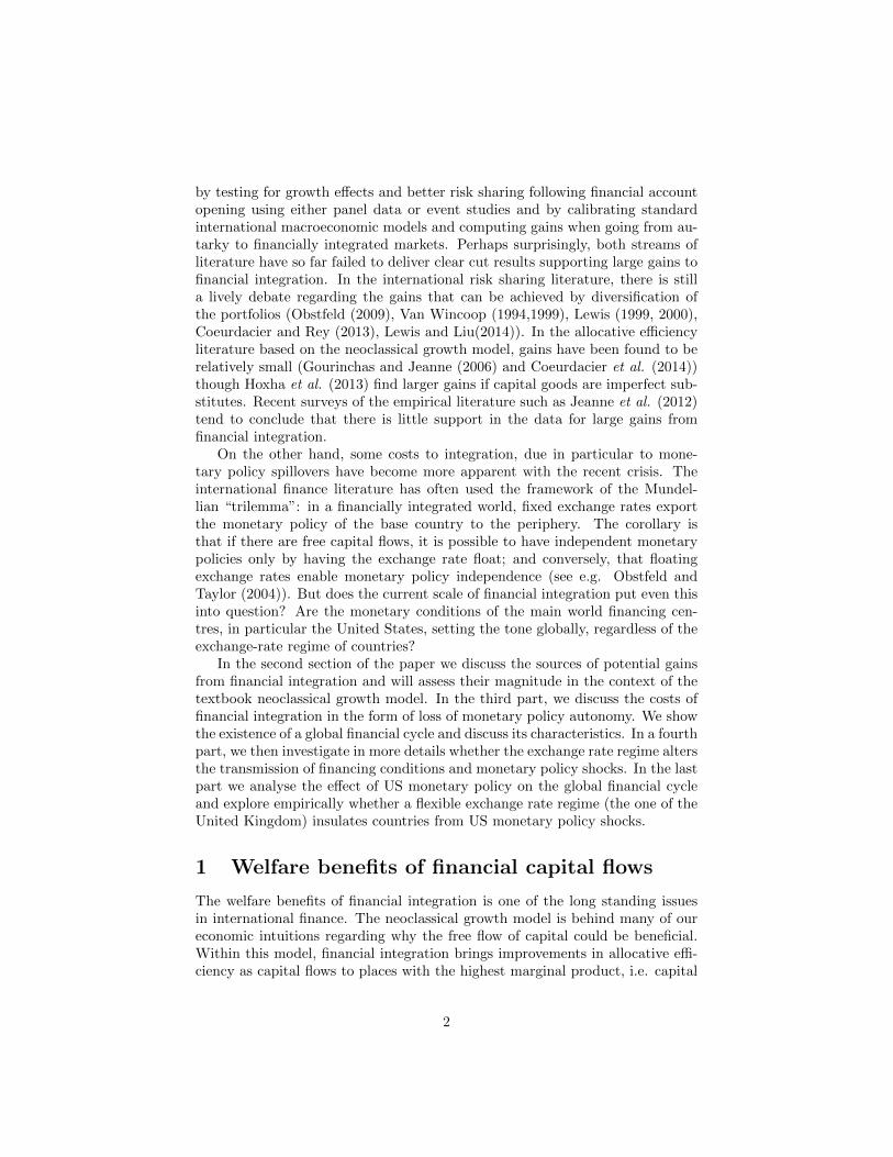
Figure 1, taken from the analysis of Coeurdacier et al. (2014), illustratesthe time paths of consumption and capital for an emerging market which iscapital scarce (hence far away from its steady state) and a developed economywhose capital stock is already at its steady state. Otherwise the environment isfully symmetric, factor markets are competitive, labour is in fixed supply andthere is no uncertainty. Dotted lines denote the autarky states while continuouslines denote the paths after financial integration (a riskless bond can be tradedinternationally). Time is measured in years on the horizontal axis. The economyis a deterministic two-country neo classical growth model (for details on themodel and calibration and a stochastic version see Coeurdacier et al. (2014)).The upper right panel shows that the time path of capital accumulation for theemerging market, when there is financial integration, is above the autarky pathin the transition period before it reaches its steady state level. The steady statelevel of capital is the same under financial integration and under autarky.3 Thegains to financial integration are thus limited to the area between the two curvesand turn out to be quantitatively quite small. The developed country gains fromfinancial integration, but also quantitatively in a very small way. As shown inthe lower right panel, it starts by exporting capital to the emerging market (thusaccumulating net claims on the emerging markets). Hence the consumption ofthe emerging market (upper left panel) is at first above its autarky level but thenbeneath it as it needs to repay its liabilities to the mature economy. The mirrorimage is true for the advanced economy which benefits in the long run froma higher consumption level than under autarky (lower left panel). The world
2See also Obstfeld and Rogoff (1996), chapter 1.3As analysed in Coeurdacier et al. (2014), this is no longer true in a stochastic world with
many interesting consequences.
3
interest rate establishes itself in between the two autarky rates of interest.When calibrated to standard values used in the literature, the welfare gains
are found to be small, of the order of a few tenths of a % of permanent consump-tion. They are even smaller than in the Gourinchas and Jeanne (2006) smallopen economy paper as a general equilibrium effect via movements in the worldrate tends to dampen welfare gains: the emerging market welfare is negativelyaffected by the world interest rate going up following integration, as it is a netdebtor to the rest of the world.
The model described here however is deterministic (as in Gourinchas andJeanne (2006)) and cannot therefore be used to analyse the welfare gains linkedto international risk sharing. Financial integration enables better risk sharing,as long as countries idiosyncratic risks are not perfectly positively correlated.4
Coeurdacier et al. (2014) are the first ones to compute welfare gains alongthe transition path in a more general neo classical growth model in a stochasticsetting, allowing for asymmetries in risk and in capital scarcity. They show thatgains from increased allocative efficiency and from risk sharing are intertwinedin interesting ways and that they can generate very rich and non monotonicpatterns of international capital flows over time. Their model can for examplegenerate global imbalances (capital flowing from the emerging market to thedeveloped economy) without any additional friction. They conclude howeverthat welfare gains of financial integration remain relatively small even in thatbroader setting and even when they consider models with realistic risk premia.
[FIGURE 1 ABOUT HERE]
There are other channels through which financial integration could be ben-eficial. It could have direct effects on Total Factor Productivity via financialmarkets development or institutional changes. It could discipline macroeco-nomic policies. We still lack convincing empirical evidence on these channelshowever (see the survey of Jeanne et al. (2012)), which constitutes an interest-ing agenda for further research. Since the large empirical literature on financialintegration is still inconclusive as well, at this stage, one can therefore sum-marise our view by stating that large gains from financial integration cannot betaken for granted.
2 Financial Integration and the Global Finan-cial Cycle
Some costs to financial integration, due in particular to monetary policy spillovershave become more apparent in the run up of and during the 2007 crisis. The
4Baxter and Crucini (1995) study the effect of different asset market structures on thecorrelations of aggregate macroeconomic variables around the deterministic steady state. Theyshow that the persistence of TFP shocks is an important parameter.
4
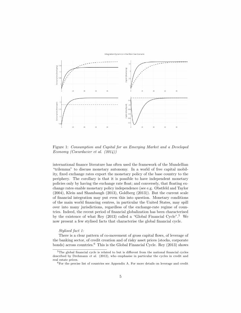
Figure 1: Consumption and Capital for an Emerging Market and a DevelopedEconomy (Coeurdacier et al. (2014))
international finance literature has often used the framework of the Mundellian“trilemma” to discuss monetary autonomy. In a world of free capital mobil-ity, fixed exchange rates export the monetary policy of the base country to theperiphery. The corollary is that it is possible to have independent monetarypolicies only by having the exchange rate float; and conversely, that floating ex-change rates enable monetary policy independence (see e.g. Obstfeld and Taylor(2004), Klein and Shambaugh (2013), Goldberg (2013)). But the current scaleof financial integration may put even this into question. Monetary conditionsof the main world financing centres, in particular the United States, may spillover into many jurisdictions, regardless of the exchange-rate regime of coun-tries. Indeed, the recent period of financial globalization has been characterisedby the existence of what Rey (2013) called a “Global Financial Cycle”.5 Wenow present a few stylised facts that characterise the global financial cycle.
Stylised fact 1:There is a clear pattern of co-movement of gross capital flows, of leverage of
the banking sector, of credit creation and of risky asset prices (stocks, corporatebonds) across countries.6 This is the Global Financial Cycle. Rey (2013) shows
5The global financial cycle is related to but is different from the national financial cyclesdescribed by Drehmann et al. (2012), who emphasise in particular the cycles in credit andreal estate prices.
6For the precise list of countries see Appendix A. For more details on leverage and credit
5
that gross inflows across geographical areas and across asset classes (credit,portfolio debt and equity, FDI) are overwhelmingly positively correlated.
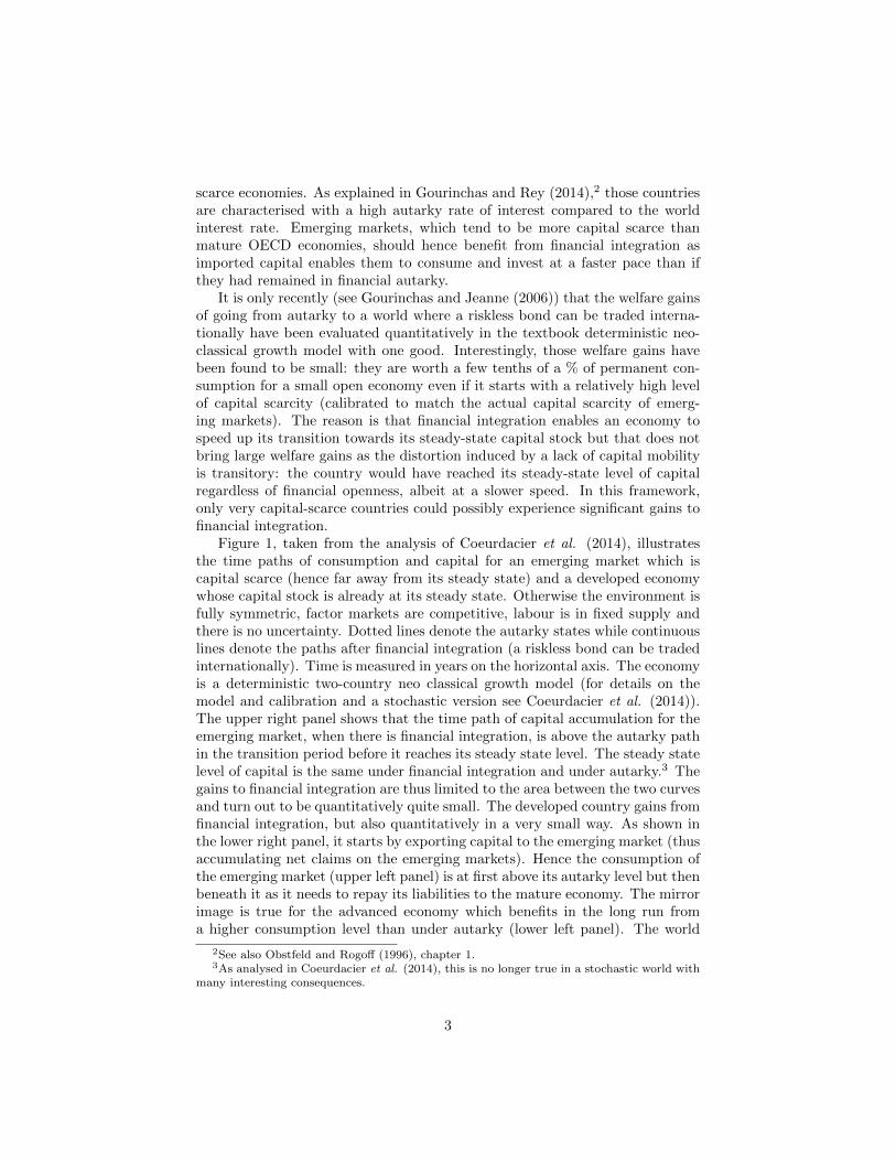
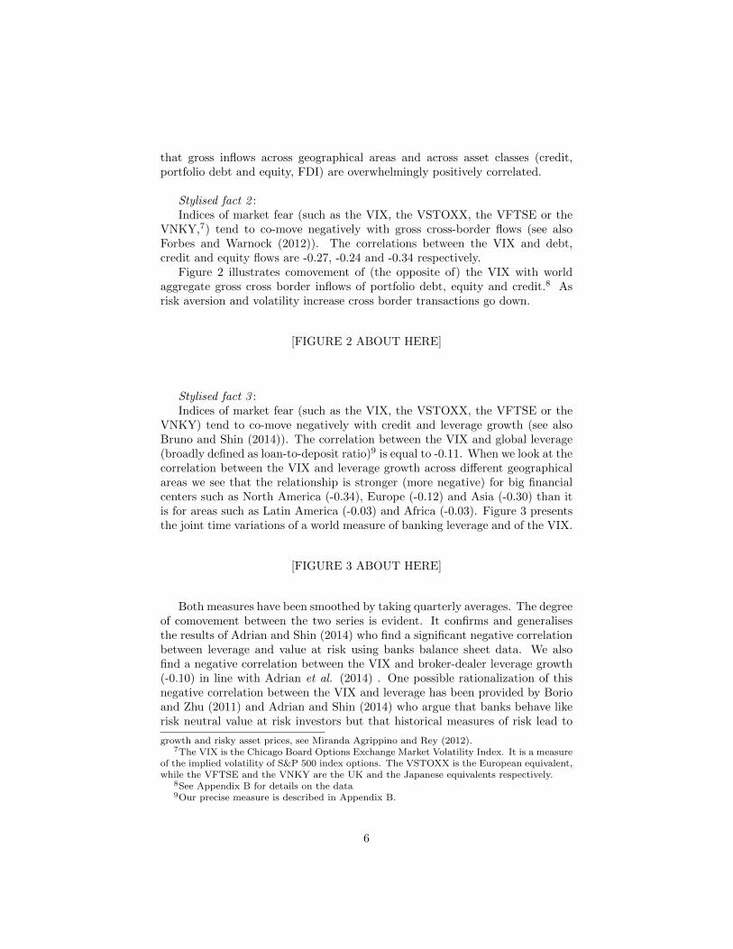
Stylised fact 2 :Indices of market fear (such as the VIX, the VSTOXX, the VFTSE or the
VNKY,7) tend to co-move negatively with gross cross-border flows (see alsoForbes and Warnock (2012)). The correlations between the VIX and debt,credit and equity flows are -0.27, -0.24 and -0.34 respectively.
Figure 2 illustrates comovement of (the opposite of) the VIX with worldaggregate gross cross border inflows of portfolio debt, equity and credit.8 Asrisk aversion and volatility increase cross border transactions go down.
[FIGURE 2 ABOUT HERE]
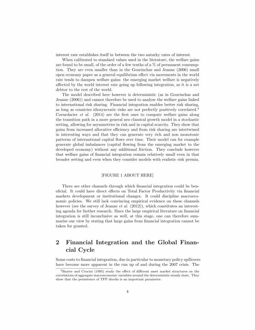
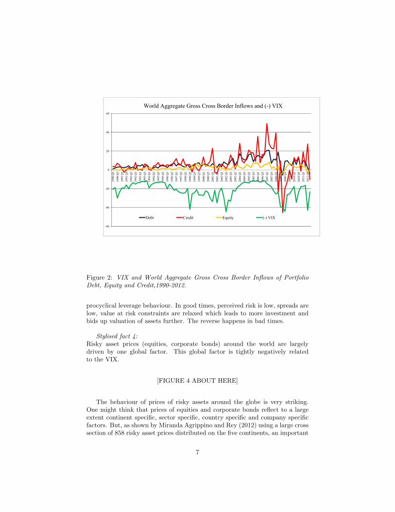
Stylised fact 3 :Indices of market fear (such as the VIX, the VSTOXX, the VFTSE or the
VNKY) tend to co-move negatively with credit and leverage growth (see alsoBruno and Shin (2014)). The correlation between the VIX and global leverage(broadly defined as loan-to-deposit ratio)9 is equal to -0.11. When we look at thecorrelation between the VIX and leverage growth across different geographicalareas we see that the relationship is stronger (more negative) for big financialcenters such as North America (-0.34), Europe (-0.12) and Asia (-0.30) than itis for areas such as Latin America (-0.03) and Africa (-0.03). Figure 3 presentsthe joint time variations of a world measure of banking leverage and of the VIX.
[FIGURE 3 ABOUT HERE]
Both measures have been smoothed by taking quarterly averages. The degreeof comovement between the two series is evident. It confirms and generalisesthe results of Adrian and Shin (2014) who find a significant negative correlationbetween leverage and value at risk using banks balance sheet data. We alsofind a negative correlation between the VIX and broker-dealer leverage growth(-0.10) in line with Adrian et al. (2014) . One possible rationalization of thisnegative correlation between the VIX and leverage has been provided by Borioand Zhu (2011) and Adrian and Shin (2014) who argue that banks behave likerisk neutral value at risk investors but that historical measures of risk lead to
growth and risky asset prices, see Miranda Agrippino and Rey (2012).7The VIX is the Chicago Board Options Exchange Market Volatility Index. It is a measure
of the implied volatility of S&P 500 index options. The VSTOXX is the European equivalent,while the VFTSE and the VNKY are the UK and the Japanese equivalents respectively.
8See Appendix B for details on the data9Our precise measure is described in Appendix B.
6
60
World Aggregate Gross Cross Border Inflows and (-) VIX
40
20
0
0 Q
10
Q3
1 Q
11
Q3
2 Q
12
Q3
3 Q
13
Q3
4 Q
14
Q3
5 Q
15
Q3
6 Q
16
Q3
7 Q
17
Q3
8 Q
18
Q3
9 Q
19
Q3
0 Q
10
Q3
1 Q
11
Q3
2 Q
12
Q3
3 Q
13
Q3
4 Q
14
Q3
5 Q
15
Q3
6 Q
16
Q3
7 Q
17
Q3
8 Q
18
Q3
9 Q
19
Q3
0 Q
10
Q3
1 Q
11
Q3
-20
1990
1990
1991
1991
1992
1992
1993
1993
1994
1994
1995
1995
1996
1996
1997
1997
1998
1998
1999
1999
2000
2000
2001
2001
2002
2002
2003
2003
2004
2004
2005
2005
2006
2006
2007
2007
2008
2008
2009
2009
2010
2010
2011
2011
-40
D bt C dit E it ( ) VIX
-60
Debt Credit Equity (-) VIX
Figure 2: VIX and World Aggregate Gross Cross Border Inflows of PortfolioDebt, Equity and Credit,1990-2012.
procyclical leverage behaviour. In good times, perceived risk is low, spreads arelow, value at risk constraints are relaxed which leads to more investment andbids up valuation of assets further. The reverse happens in bad times.
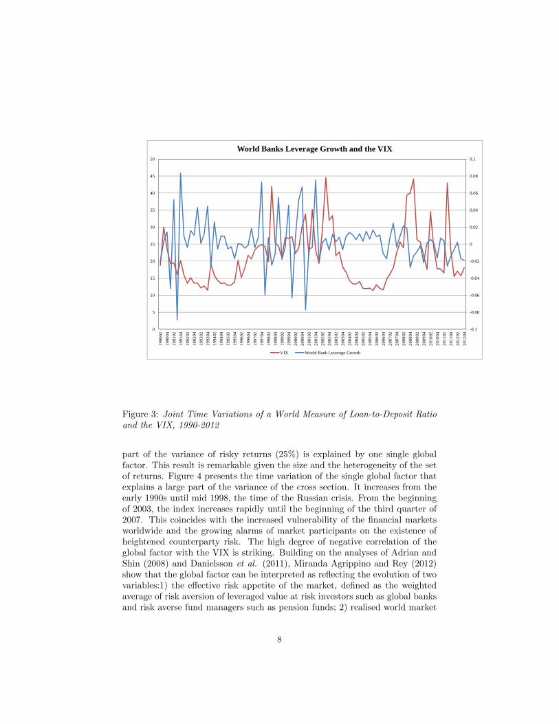
Stylised fact 4:Risky asset prices (equities, corporate bonds) around the world are largelydriven by one global factor. This global factor is tightly negatively relatedto the VIX.
[FIGURE 4 ABOUT HERE]
The behaviour of prices of risky assets around the globe is very striking.One might think that prices of equities and corporate bonds reflect to a largeextent continent specific, sector specific, country specific and company specificfactors. But, as shown by Miranda Agrippino and Rey (2012) using a large crosssection of 858 risky asset prices distributed on the five continents, an important
7
-0 02
0
0.02
0.04
0.06
0.08
0.1
20
25
30
35
40
45
50
World Banks Leverage Growth and the VIX
-0.1
-0.08
-0.06
-0.04
-0.02
0
5
10
15
20
1990
0219
9004
1991
0219
9104
1992
0219
9204
1993
0219
9304
1994
0219
9404
1995
0219
9504
1996
0219
9604
1997
0219
9704
1998
0219
9804
1999
0219
9904
2000
0220
0004
2001
0220
0104
2002
0220
0204
2003
0220
0304
2004
0220
0404
2005
0220
0504
2006
0220
0604
2007
0220
0704
2008
0220
0804
2009
0220
0904
2010
0220
1004
2011
0220
1104
2012
0220
1204
VIX World Bank Leverage Growth
Figure 3: Joint Time Variations of a World Measure of Loan-to-Deposit Ratioand the VIX, 1990-2012
part of the variance of risky returns (25%) is explained by one single globalfactor. This result is remarkable given the size and the heterogeneity of the setof returns. Figure 4 presents the time variation of the single global factor thatexplains a large part of the variance of the cross section. It increases from theearly 1990s until mid 1998, the time of the Russian crisis. From the beginningof 2003, the index increases rapidly until the beginning of the third quarter of2007. This coincides with the increased vulnerability of the financial marketsworldwide and the growing alarms of market participants on the existence ofheightened counterparty risk. The high degree of negative correlation of theglobal factor with the VIX is striking. Building on the analyses of Adrian andShin (2008) and Danielsson et al. (2011), Miranda Agrippino and Rey (2012)show that the global factor can be interpreted as reflecting the evolution of twovariables:1) the effective risk appetite of the market, defined as the weightedaverage of risk aversion of leveraged value at risk investors such as global banksand risk averse fund managers such as pension funds; 2) realised world market
8
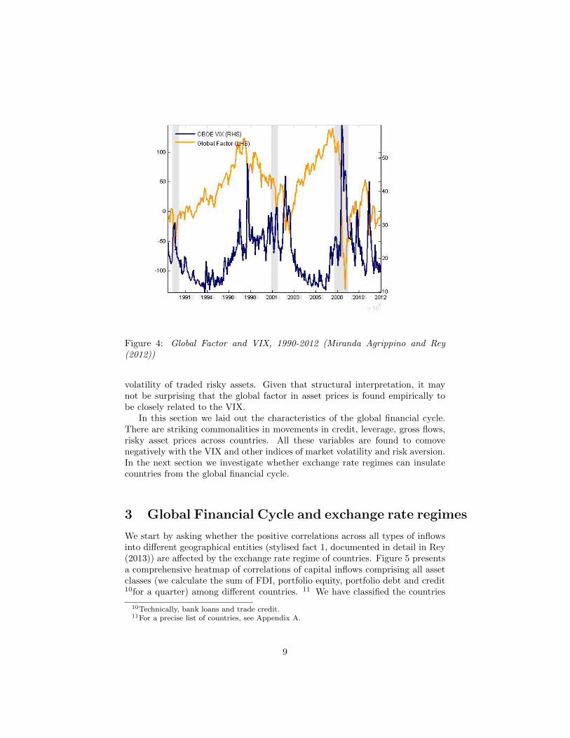
Figure 3: Global factor and VIX. Source: Miranda‐Agrippino and Rey (2012).
To sum up, we have now established in flow data (across most types of flows and regions, but with
some exceptions) and in price data (across a sectorally and geographically wide cross‐section of risky
asset prices) the existence of a global financial cycle. Interestingly, the VIX is a powerful index of the
global financial cycle, whether for flows or for returns. Our analysis so far emphasizes striking
correlations and patterns, but cannot address causality issues. Low value of the VIX, in particular for
long periods of time, are associated with a build up of the global financial cycle: more capital inflows
and outflows, more credit creation, more leverage and higher asset price inflation.
III)Capitalflowsandmarketsensitivitiestotheglobalfinancialcycle
In this part I attempt to gauge further the importance of the global financial cycle for different asset
markets (stock prices, house prices) as well as for the leverage of financial intermediaries. Having
reported the importance of the global cycle for the fluctuations of these variables in the time series
dimension, I study in more details the factors affecting the cross sectional sensitivities of these
variables to the global financial cycles. More precisely, I focus here on the possibility that larger
Figure 4: Global Factor and VIX, 1990-2012 (Miranda Agrippino and Rey(2012))
volatility of traded risky assets. Given that structural interpretation, it maynot be surprising that the global factor in asset prices is found empirically tobe closely related to the VIX.
In this section we laid out the characteristics of the global financial cycle.There are striking commonalities in movements in credit, leverage, gross flows,risky asset prices across countries. All these variables are found to comovenegatively with the VIX and other indices of market volatility and risk aversion.In the next section we investigate whether exchange rate regimes can insulatecountries from the global financial cycle.
3 Global Financial Cycle and exchange rate regimes
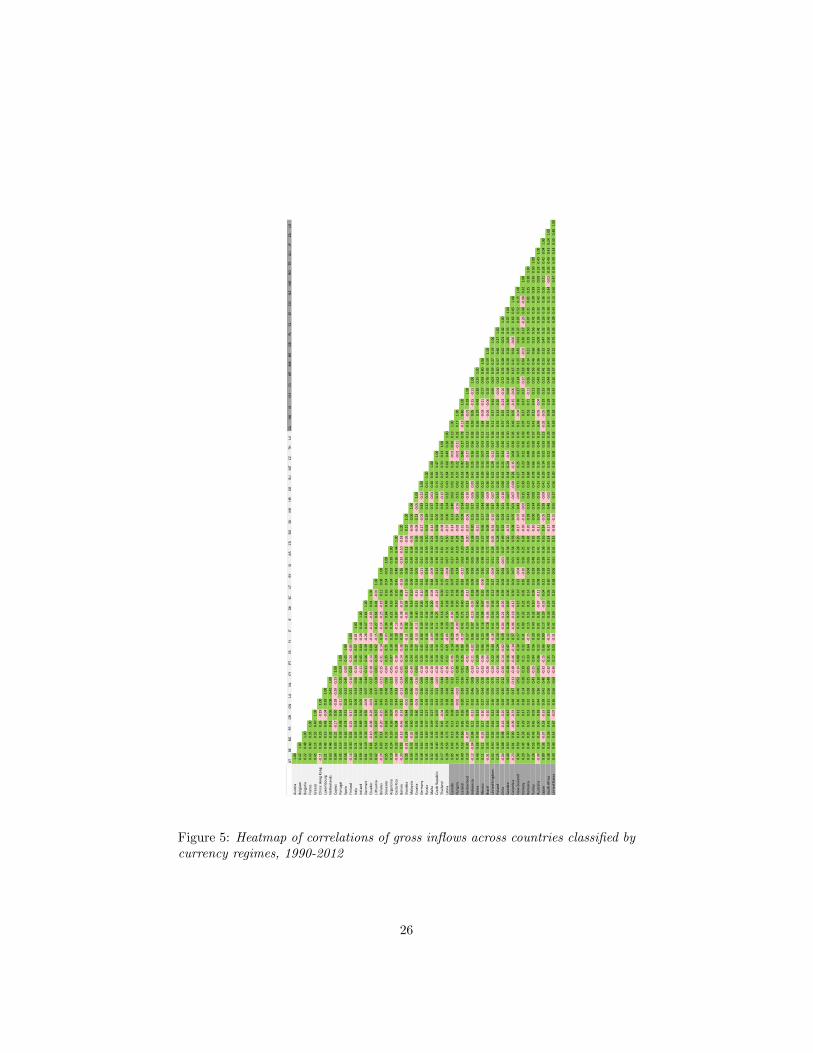
We start by asking whether the positive correlations across all types of inflowsinto different geographical entities (stylised fact 1, documented in detail in Rey(2013)) are affected by the exchange rate regime of countries. Figure 5 presentsa comprehensive heatmap of correlations of capital inflows comprising all assetclasses (we calculate the sum of FDI, portfolio equity, portfolio debt and credit10for a quarter) among different countries. 11 We have classified the countries
10Technically, bank loans and trade credit.11For a precise list of countries, see Appendix A.
9
by exchange rate regime, the darker shades corresponding to floating regimesand the lighter shades corresponding to fixed regimes. The data for the flowsare quarterly ranging between the first quarter of 1990 and the last quarter of2012 and come from the IMF International Financial Statistics database. Theexchange rate regime data are taken from the update of the monthly de factoexchange rate regime classification of Reinhart and Rogoff (2004) by Ilzetzki andReinhart (2009). The exchange rate regime is multilateral; we do not considerbilateral regimes vis-a-vis the US dollar (though that would be an interestinganalysis to perform in itself) as monetary policy autonomy is impeded as soonas the exchange rate is not freely floating irrespective of the base currency acountry pegs to. Hence, euro area countries have a rigid exchange rate regimefor a large part of the sample despite the fact that the euro floats against theUS dollar. The Reinhart and Rogoff coarse classification ranges from 1 to 6,the lower numbers corresponding to the more fixed exchange rates with thehigher numbers corresponding to free floaters up till 4.12 We exclude categories5 (freely falling currencies) and 6 (dual market in which parallel market datais missing) due to the small number of observations available. Our regimevariable therefore takes the values 1,2,3 and 4, where lower values suggest amore rigid regime. The exchange rate regime variable is time varying and weuse it as such in the panel regressions below. But for the heatmap we averageits value over the sample and use this time series average value to rank ourcountries according to the degree of rigidity of their exchange rate regime. Theheatmap thus presents the correlation of gross inflows across countries classifiedaccording to the average degree of rigidity of their exchange rate system over theperiod (darker colours are the floaters). Correlations are green when positiveand red when negative. As evidenced by the very clear preponderance of thegreen colour in the heatmaps, most gross capital inflows are positively correlatedacross countries. What is remarkable is that the pattern of correlations doesnot seem to be noticeably affected by the exchange rate regime. There is nodifference between the correlations involving the more flexible exchange ratecountries (darker shades) and the others.
[FIGURE 5 ABOUT HERE]
We now investigate more formally whether the exchange rate regime affectsmaterially the transmission of the financial cycle to countries, i.e. whether the
12In particular, 1 denotes no separate legal tender, a pre announced peg or a currency boardarrangement, a pre announced horizontal band that is narrower than or equal to +/-2% ora de facto peg; 2 stands for announced crawling peg, pre announced crawling band that isnarrower than or equal to +/-2%, de facto crawling peg, or de facto crawling band that isnarrower than or equal to +/- 2%; 3 denotes pre announced crawling band that is wider thanor equal to +/- 2%, de facto crawling band that is narrower than or equal to +/-5%, movingband that is narrower than or equal to +/-2% or managed floating currency regime and 4stands for freely floating currency regime. Details on the classification are shown in AppendixB.
10
correlations between stock market prices and credit growth are not correlatedwith the VIX (our proxy for the Global Financial Cycle) when countries havea flexible exchange rate regime. Indeed, floating rates can in principle ensuremonetary policy autonomy and insulate countries from foreign influences. Aseries of papers by Obstfeld et al. (2005), Klein and Shambaugh (2013), Gold-berg (2013), Obstfeld (2014) have consistently found that short rates are lesscorrelated to the base country rate for flexible exchange rate countries thanfor fixed exchange rate countries. Indeed policy rates are freer to move underfloating rates than under fixed rates. It remains to be seen however whethermovements in the policy rates are able to affect monetary and financial condi-tions significantly and provide insulation from the Global Financial Cycle (for amore precise discussion see Rey (2014)). Interestingly, Obstfeld (2014) finds thatcorrelations in the long rates are unaffected by exchange rate regimes, suggest-ing a very imperfect ability of the policy rate to set country specific monetaryconditions for longer term investment. In this paper, we present some comple-mentary evidence. The pattern of comovements of gross inflows does not seemto be materially affected by the regime, as the heatmap shows. Additionally, weinvestigate whether cross sectionally, the sensitivities of the local stock marketand of credit growth to the Global Financial Cycle (proxied by the VIX) areaffected by the exchange rate regime. In order to do so, we run panel regressionsof stock prices on one hand and credit growth on the other hand on the VIXand the VIX interacted with exchange rate regime dummies, the Fed Funds rate(allowing also for interactions) and some control variables.
3.1 Panel regressions
We denote by ff t the Federal Funds Rate, vixt the VIX (logged), ∆vixt itsfirst difference, si,t the stock market return of country i measured by the end ofperiod return of the country’s main stock market index excluding dividends, ci,tthe credit growth in country i and by xi,t and yt control variables which maybe country specific. Our panel comprises 53 countries (see Appendix A) andthe times series ranges between the first quarter of 1990 and the last quarterof 2012. Dummy variables for exchange rate regimes are denoted by ri withi ∈ {1; 2; 3; 4} where the low numbers denote fixed regimes and high numbersdenote the floating regimes, using the Reinhart and Rogoff classification updateas described above. We use the following specifications:13
si,t = αi + βvixt +∑
i∈{1;2;3;4}
γiri.vixt + δ∆vixt +∑
i∈{1;2;3;4}
ηiri.∆vixt +
θff t +∑
i∈{1;2;3;4}
κiri.ff t + λxi,t−1 + µyt−1 + εi,t (1)
13For a model that microfounds the use of the VIX and VIX growth rate in a regressionto explain credit creation see Bruno and Shin (2014). For another application see MirandaAgrippino and Rey (2013). The data are available online.
11
ci,t = αi + βvixt +∑
i∈{1;2;3;4}
γiri.vixt + δ∆vixt +∑
i∈{1;2;3;4}
ηiRi.∆V IXt +
θff t +∑
i∈{1;2;3;4}
κiri.ff t + λxi,t−1 + µyt−1 + εi,t (2)
Control variables are the lagged world GDP growth rate yt−1 and the laggedcountry GDP xi,t−1. The dummy interaction terms serve the purpose of cap-turing the potential heterogeneous sensitivity of a given market to US monetarypolicy and to the Global Financial Cycle (proxied by the VIX) depending onthe exchange rate regime. We run fixed effects estimators with clustered stan-dard errors by country. We have a large number of observations (between 1066and 3982 depending on the specification). Tables 1 and 2 report the resultsof the regression for stock market returns (log difference of local stock marketindices) and for credit growth (log difference in credit over GDP) respectively.For each regression we use monthly data over the 1990-2013 period and we splitthe sample in three subperiods: up to the crisis (1990 until 2007); the run upto the crisis (2000 until 2007) and the crisis period (2007-2013).
Table 1 shows the estimated parameter coefficients for the VIX, the changein the VIX and the Fed Funds rate. Stock returns are significantly negativelyrelated to the VIX in all subperiods. The interaction terms between the FedFunds Rate and the currency regime and the VIX (in log level and difference)and the currency regime denote the difference in the slopes of the benchmarkcase (pegged exchange rate regime, category 1 of Reinhart and Rogoff) andthe slope of regimes 2, 3 and 4. Although some of the VIX exchange rateregime interactions are positive and significant, there is no pattern that couldbe linked to degree of exchange rate flexibility as there is great heterogeneityin the results across periods and across regimes. The only subperiods for whichthe flexible regime (4) is associated with a positive interaction term are the2000-2007 and the 2007-2013 subperiods and during these periods the overallcorrelation between the VIX and the stock returns is still negative. Similarly,whenever the interaction term between the exchange rate regime and the VIXis positive elsewhere (for example for regime 2 during 1990-2007), the overalleffect remains negative. The change in VIX is also negatively related to thestock returns, with some positive interaction terms for the flexible exchangerates (regime 4) but also for relatively fixed rates (regime 2). The Fed Fundsrate tends to be either positively associated with stock returns or insignificant.However, most interaction terms are negative and reverse the positive correlationto a negative one for most exchange rate regimes. Hence, more rigid regimes donot seem to be associated with a higher sensitivity of the stock market of countryi to the Global Financial Cycle (or to the Fed Funds rate) in a systematic way.
[TABLE 1 ABOUT HERE]
Domestic credit growth (Table 2) is significantly negatively related to theVIX in all subperiods except the crisis (2007-2013) where it is positively related
12
in levels but negatively related in difference. There is again no systematic re-lation between the VIX and the currency regime though the interaction termwith the more flexible regime (4) and with the relatively fixed exchange rateregime (2) is again significant in some subperiods (without overturning the signof the overall negative correlation). The correlation with the Fed Funds rate ispositive and sometimes significant. Once again, there does not seem to be sys-tematic evidence that more rigid regimes are associated with a higher sensitivityof credit growth in country i to the US monetary policy or to the VIX.
It is very important to realise that the panel regressions of this section indi-cate only correlations and do not imply the existence of any form of causality.They are meant to illustrate cross sectional comovements with the Global Finan-cial Cycle across different exchange rate regimes. To summarise our results, wefind that although there is some degree of heterogeneity in the sensitivities, noexchange rate regime seems to be systematically associated with a significantlylower sensitivity to the global financial cycle.
[TABLE 2 ABOUT HERE]
4 Global Financial cycle and US monetary pol-icy
A natural next step in our investigation is to analyse the potential drivers ofthe global financial cycle. Given the importance of the US Dollar on interna-tional financial markets (see Portes and Rey (1998) Shin (2013)), one primecandidate is US monetary policy. In the domestic context financial market im-perfections have been shown to be important for the transmission of monetarypolicy: in the “credit channel” (Bernanke and Gertler (1995)), agency costscreate a wedge between the costs of external finance and internal funds. Thiswedge depends on the net worth of firms, banks, households or on value at riskconstraints (see Adrian and Shin (2014), Bruno and Shin (2014), Borio andZhu (2011)) and therefore inter alia on monetary policy. As Rey (2014) pointsout, the international role of the dollar as a funding currency and as an in-vestment currency suggests that US monetary policy by affecting the net worthof investors, intermediaries and firms worldwide may transmit US monetaryconditions across borders and jurisdictions. Hence, the existence of an ”inter-national credit channel” that propagates the global financial cycle. In order toinvestigate empirically the nature of such a transmission mechanism, we needto evaluate the combined responses of a set of economic and financial variablessuch as mortgage spreads, which are a measure of the external finance premiumto US monetary policy surprises.
As underlined by Stock and Watson (2008, 2012), the identification problemin structural VAR analysis is how to go from the moving-average representation
13
in terms of the innovations to the impulse response function with respect to aunit increase in the structural shock of interest, which is here the US mone-tary policy shock. Traditionally, imposing economic restrictions such as timingrestrictions (some variables move within the month, others are slower mov-ing) have permitted identification of the coefficients (see Bernanke and Gertler(1994), Christiano et al. (1996).)14 When one tries to identify the internationalcredit channel of monetary policy, movements in asset prices and spreads arekey, as they are related to the external finance premium or the operation ofvalue at risk constraints. Hence, it is of the utmost importance to use an iden-tification strategy which allows for immediate response in asset prices, as thereis certainly no delay in those market reactions. We follow Gertler and Karadi(2014) whose approach brings together vector autoregression (VAR) analysisand high frequency identification (HFI) of monetary policy shocks and use theGurkaynak et al.(2005) surprise measures as external instruments in our VAR.15
These are very clever instruments as they measure surprises as changes in Fedfunds futures in tight windows around monetary policy announcement times.As Fed funds future prices aggregate all available information about expectedmonetary policy rates prior to FOMC meetings, any change in their prices atthe time of the meeting is very likely reflecting only a monetary policy surprise.It is indeed unlikely that any other event dominates fluctuations in the pricesof Fed funds futures in a 30 minute or 15 minute window around the announce-ment. Their approach addresses the simultaneity issue of monetary policy shifts,which influence and at the same time respond to financial variables. FollowingGertler and Karadi (2014), we use these surprises to instrument the one yearUS interest rate in our VAR. The advantage of instrumenting the one year rate(as opposed to the Fed Funds rate) is that the effect of forward guidance canbe taken into account in the estimates. This is of course particularly importantin a period where the Fed Funds rate has hit the zero lower bound.
4.1 Methodology
Our vector autoregression contains both economic and financial variables. Toidentify monetary surprises we use external instruments following the method-ology developed by Mertens and Ravn (2013).16 Let,
Agt =m∑
k=1
Ckgt−k + εt (3)
be our general structural form. The reduced form representation can be thenwritten as follows:
14As is well known, Romer and Romer (1989, 2004) introduce what has been called the”narrative approach”, that is to say use information from outside the VAR to constructexogenous components of specific shocks.
15For another recent study where external instruments are used to identify the structuralshocks of a VAR in the case of fiscal policy see Mertens and Ravn (2013).
16See also Stock and Watson (2012). The program is available online.
14
gt =m∑
k=1
Dkgt−k + ut, (4)
where the reduced form shock ut is a function of the structural shocks:ut = Pεt, where Dk = A−1Ck and P = A−1.
We define Σ the variance-covariance matrix of the reduced form model. ForΣ, we have:
Σ = E[utu′
t] = E[PP′]. (5)
We assume gmt ∈ gt, to be the monetary policy indicator, and in particularthe US government bond rate with one-year maturity as discussed in the pre-vious section. The exogenous variation of the policy indicator stems from thepolicy shock εmt .
Finally, p stands for the column in P corresponding to the impact of thepolicy shock εmt on each element of the vector of reduced form residuals ut. Forthe impulse responses of our economic and financial variables to a policy shockwe run:
gt =m∑
k=1
Dkgt−k + pεmt . (6)
As discussed in the previous section, standard timing restrictions are prob-lematic in the presence of financial variables. For this reason, we follow theidentification strategy of Gertler and Karadi (2014) and employ their externalinstruments. In order for the vector of instrumental variables zt to be a validset of instruments for the monetary policy shock εmt we need:
E[ztεm′
t = Φ] (7)
and
E[ztεd′
t = 0], (8)
where εdt stands for any structural shock but the monetary policy shock.In order to compute the estimates of vector p, as a first step we need to
compute the estimates of the reduced form residuals vector ut from the leastsquares regression of the reduced form representation. We denote ud
t the re-duced form residual from the equation for variable d which is different from thepolicy indicator and um
t the reduced form residual from the equation for thepolicy indicator. Additionally, assume that pd ∈ p is the response of ud
t to aunit increase of one standard deviation in the policy shock εmt . From the twostage least squares regression of ud
t on umt and using the vector of instrumental
variables zt, one can compute an estimate of the ratio pd/pm. 17
17In particular, the variation in the reduced form residual for the policy indicator due to thestructural policy shock is first isolated by regressing um
t on the vector of instruments yielding
15
4.2 Results
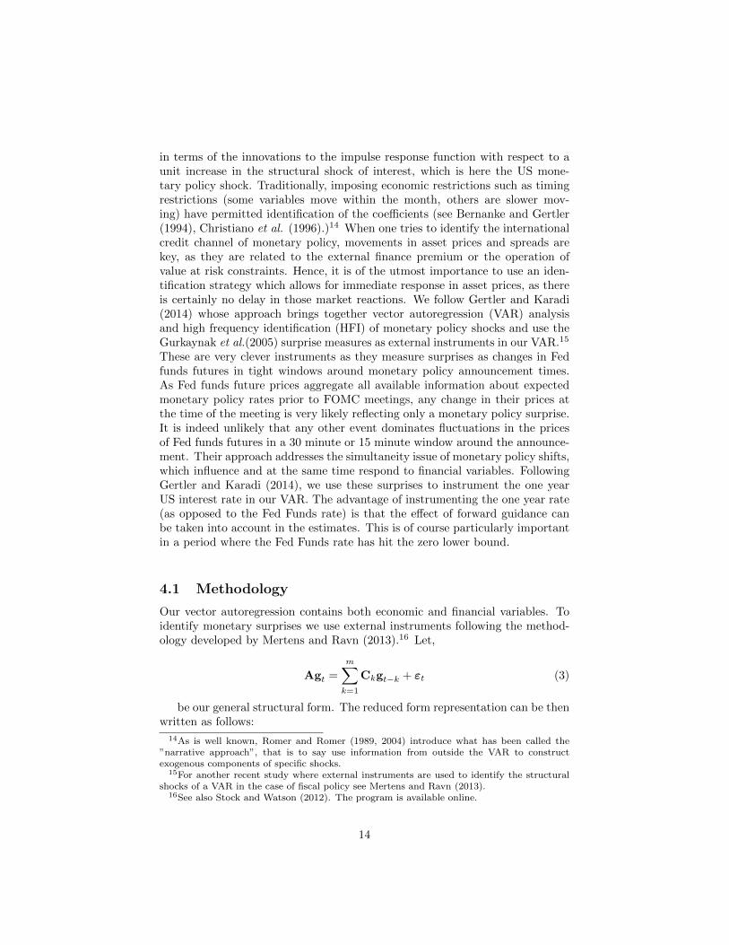
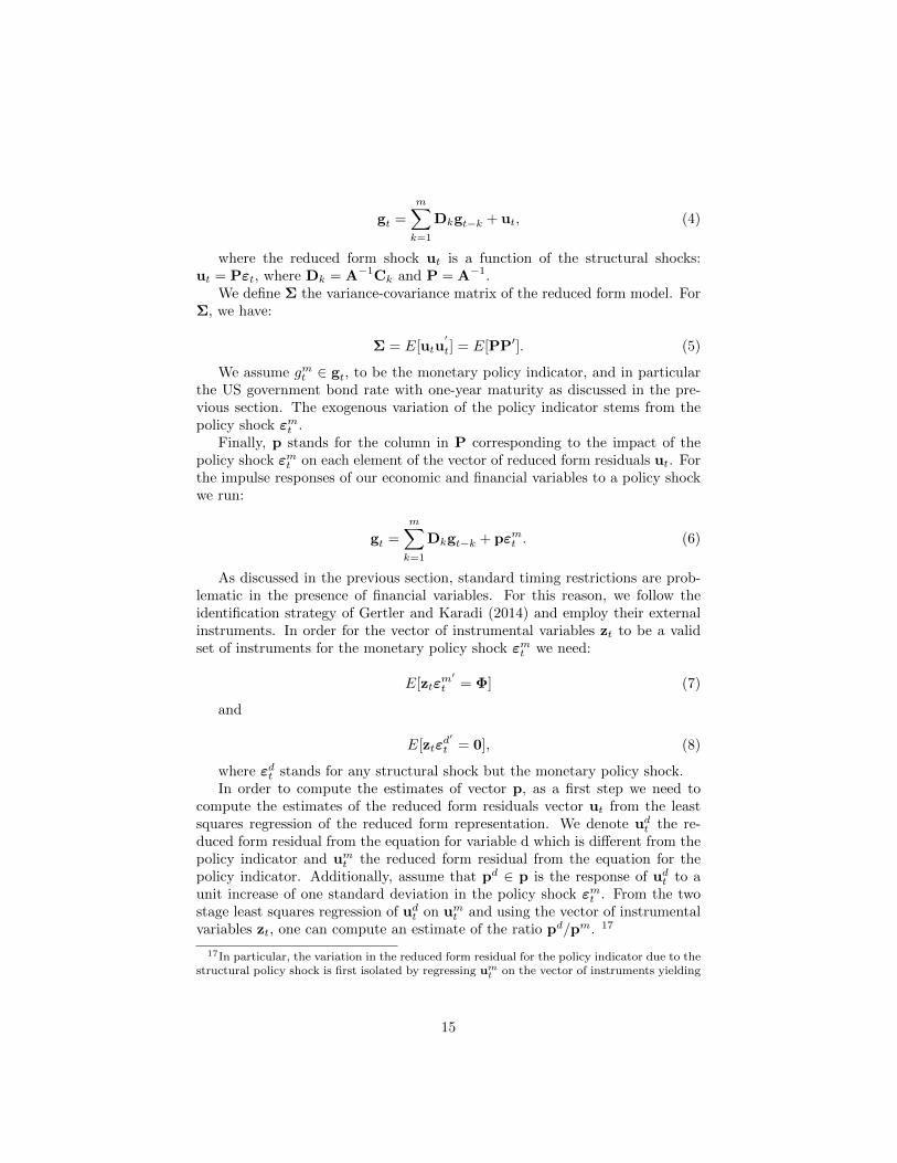
We analyse the effect of US monetary policy shocks on the global financial cycle(through the VIX) as well as on the US external finance premium. We thenstudy the effect of US monetary policy shocks on a mostly floating exchange rateeconomy (the UK). According to the traditional Mundell Fleming model andthe trilemma, the UK should be insulated from US monetary policy spillovers bymovements in the dollar pound rate and should be able to set its own monetaryand financial conditions. Our empirical strategy allows us to test whether the”international credit channel” is potent enough to put this classic idea intoquestion.18
US monetary policy and the Global Financial CycleWe consider a monthly VAR on data ranging between 1979 and 2012, that
includes real economy variables such as US industrial production (seasonallyadjusted) and the US CPI as well as variables capturing the external financepremium (US mortgage spread and US corporate bond spread). We also includethe VIX as a proxy for the Global Financial Cycle, correlated with global lever-age, gross cross border flows and the global component in risky asset prices. Asdiscussed above, we use external instruments based on Fed Funds rate futuressurprises to identify the monetary policy shocks.19 We replicate the results ofGertler and Karadi (2014) and find (see figure 6) , for a 20 bp shock to the USone year rate a strong reaction of the mortgage spread (peak about 8 bp) andof the US corporate spread (about 6 bp). Extending our analysis to global vari-ables, we also find that a 20 bp shock in the one year rate leads to a 5 bp shockto the VIX (logged, a standard deviation in the log VIX is 15.2 bp). We readthese Impulse Response Functions as supporting the importance of the creditchannel of monetary policy both domestically and internationally. When theFederal Reserve tightens, the VIX goes up and global asset prices go down. InMiranda Agrippino and Rey (2012), we use a large Bayesian VAR with 22 vari-ables in quarterly data to study the effect of US monetary policy on the globalfinancial cycle. We use the narrative approach of Romer and Romer (2004) toidentify the monetary policy shocks. Our results also support the existence ofa significant effect of a Fed tightening on credit creation, capital flows, lever-age of global banks and external finance premia and global asset prices. It iscomforting that two very different methodologies (a small VAR with externalinstruments and a large Bayesian VAR with different external instruments) givevery consistent results.
umt . As the variation in um
t is only due to εmt , a second stage regression of udt on um
t provides
a consistent estimate of pd/pm. The estimated reduced form variance-covariance matrix isthen used to obtain an estimate of pm using the second stage regression, allowing to identifypd. For more details see Gertler an Karadi (2014) and Mertens and Ravn (2013).
18For a detailed discussion of the international credit channel and of the relevant empiricalevidence see Rey (2014).
19We are very grateful to Mark Gertler and Peter Karadi for having shared their data andinstruments very graciously.
16
[FIGURE 6 ABOUT HERE]
Figure 6: Response of the VIX to a 20bp increase in the US one year rate.Instruments from Gertler and Karadi(2014), 95% confidence intervals
US monetary policy spillovers into a floating exchange rate countryThe ubiquity of the global financial cycle and our previous panel results seem
to indicate that even flexible exchange rate regime countries are not insulatedfrom global factors, yet, it is worth exploring this important question in moredetail. We estimate directly the effect of US monetary policy shocks on activity,inflation and the external finance premium for the United Kingdom, an advancedeconomy that embraced inflation targeting. We rely on the same estimationstrategy as above. The variables in the UK VAR are industrial production,the CPI, the domestic policy rate, the mortgage spread (most widely availableseries with a long time span across countries) and the VIX. Using the mortgagespread has an additional advantage: the real estate market is central for financialstability and has been shown to be very important in boom bust cycles aroundthe world. In the domestic UK context, a 17 bp increase in the US one yearrate leads to a 8 bp increase in the mortgage spread within half a year. Inthe UK, a US tightening also has a significant effect on mortgage spreads. It
17
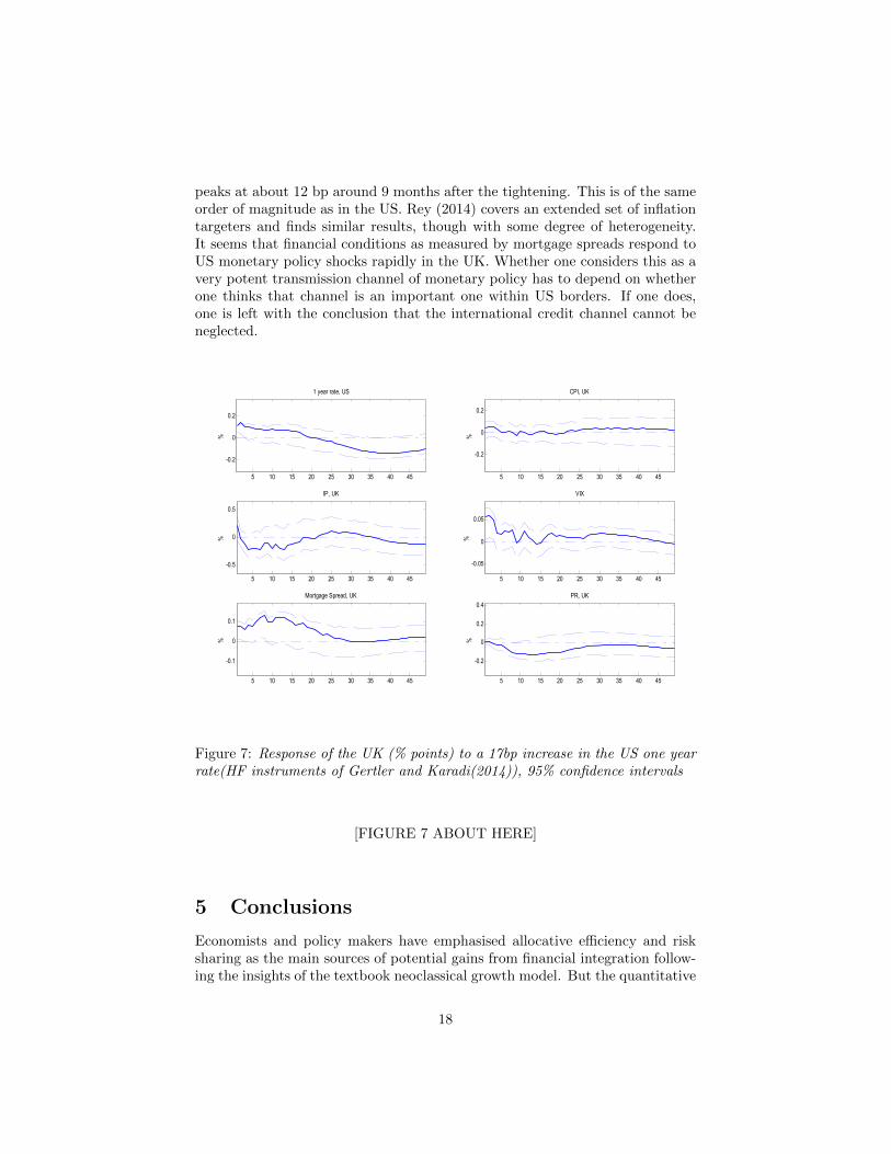
peaks at about 12 bp around 9 months after the tightening. This is of the sameorder of magnitude as in the US. Rey (2014) covers an extended set of inflationtargeters and finds similar results, though with some degree of heterogeneity.It seems that financial conditions as measured by mortgage spreads respond toUS monetary policy shocks rapidly in the UK. Whether one considers this as avery potent transmission channel of monetary policy has to depend on whetherone thinks that channel is an important one within US borders. If one does,one is left with the conclusion that the international credit channel cannot beneglected.
5 10 15 20 25 30 35 40 45
-0.2
0
0.2
%
1 year rate, US
5 10 15 20 25 30 35 40 45
-0.2
0
0.2
%
CPI, UK
5 10 15 20 25 30 35 40 45
-0.5
0
0.5
%
IP, UK
5 10 15 20 25 30 35 40 45
-0.05
0
0.05
%
VIX
5 10 15 20 25 30 35 40 45
-0.1
0
0.1
%
Mortgage Spread, UK
5 10 15 20 25 30 35 40 45
-0.2
0
0.2
0.4
%
PR, UK
Figure 7: Response of the UK (% points) to a 17bp increase in the US one yearrate(HF instruments of Gertler and Karadi(2014)), 95% confidence intervals
[FIGURE 7 ABOUT HERE]
5 Conclusions
Economists and policy makers have emphasised allocative efficiency and risksharing as the main sources of potential gains from financial integration follow-ing the insights of the textbook neoclassical growth model. But the quantitative
18
evaluation of these models shows that these gains are not very big. Togetherwith the relatively non conclusive large empirical literature on financial integra-tion, this leads us to believe that large welfare gains from financial integrationare hard to find. This is particularly striking given the scale of cross borderfinancial flows which have increased massively. Large gross cross border flowsare moving in tandem across countries regardless of the exchange rate regime,they tend to rise in periods of low volatility and risk aversion and decrease inperiods of high volatility and risk aversion, as measured by the VIX. Risky assetprices around the world are also largely driven by one global component tightlycorrelated to the VIX. Leverage and credit across countries show significant de-grees of co-movements (and are negatively correlated with the VIX). There is aglobal financial cycle. We find that the correlations of stock prices and creditgrowth with the global financial cycle (proxied by the VIX) do not seem tovary systematically with the exchange rate regime. Using a VAR methodolodywith external instruments, we also show that US monetary policy has an effecton the VIX (a US tightening increases the VIX). Importantly we find that USmonetary policy has also an effect the United Kingdom’s external finance pre-mium (measured by the mortgage spread), even though the UK has a floatingexchange rate regime. This seems to indicate that the insulating properties offloating regimes may have been overestimated. It would be desirable to estimatethe effect of a Fed tightening on other measures of financial conditions (corpo-rate spreads, effect on the term premium) and on a broader set of countries. Itwould also be important to disentangle the two main channels through whichthe dependence of UK monetary conditions (evidenced by the mortgage spreadreaction) on the policy stance of the United States could take place. The firstone is the ”fear of floating” (Calvo and Reinhart (2002)) whereby Central Banksthreatened by large capital flows could try to reduce the interest rate differentialwith the Federal Reserve. The second one is the international credit channelwhereby even if the domestic policy rate remains unaltered domestic financialconditions are affected by the change in monetary policy of the Federal Reservevia the role of the dollar as an international currency. Future research will nodoubt shed further light on these issues.20
Universite Paris DauphineLondon Business School, CEPR and NBER
20Rey (2014) makes some progress in this direction.
19
References
[1] Adrian, T., Etula, E., and Muir, T.(2014). ‘Financial Intermediaries andthe Cross-Section of Asset Returns’, Journal of Finance, vol. 69(6), pp.2557–2596.
[2] Adrian, T. and Shin, H. S.(2014). ‘Pro-cyclical Leverage and Value-at-Risk’, Review of Financial Studies, vol. 27(2), pp. 373–403.
[3] Baxter, M. and Crucini, M. J.(1995). ‘Business Cycles and the AssetStructure of Foreign Trade’, International Economic Review, vol. 36(4),pp. 821–854.
[4] Bernanke, B. and Gertler, M.(1995). ‘Inside the Black Box: The CreditChannel of Monetary Policy Transmission’, Journal of Economic Perspec-tives, vol. 9(4), pp. 27–48.
[5] Borio, C. and Zhu, H.(2011). ‘Capital regulation, risk-taking and mon-etary policy: a missing link in the transmission mechanism?’, Journal ofFinancial Stability (forthcoming).
[6] Bruno, V. and Shin, H. S.(2014). ‘Cross-Border Banking and GlobalLiquidity’, Review of Economic Studies (forthcoming).
[7] Calvo, G. A. and Reinhart, C. M.(2002). ‘Fear of Floating’, QuaterlyJournal of Economics, vol. 117(2), pp. 379–408.
[8] Christiano, L. J., Eichenbaum, M., and Evans, C.(1996). ‘The effects ofmonetary policy shocks: Evidence from the flow of funds’, The Review ofEconomics and Statistics, vol. 78(1), pp. 16–34.
[9] Coeurdacier, N. and Rey, H.(2012). ‘Home Bias in Open Economy Fi-nancial Macroeconomics’, Journal of Economic Literature, vol. 51(1), pp.63–115.
[10] Coeurdacier, N., Rey, H., and Winant, P.(2013). ‘Financial Integrationand Growth in a Risky World’, Working Paper, London Business Schooland SciencesPo.
[11] Danielsson, J., Song Shin, H., and Zigrand, J.-P.(2011). ‘Balance sheetcapacity and endogenous risk’, FMG discussion paper series, No. 665, Fi-nancial Markets Group, London School of Economics and Political Science.
[12] Drehmann, M., Borio, C., and Tsatsaronis, K.(2012). ‘Characterising thefinancial cycle: don’t lose sight of the medium term!’, BIS Working Papers,No. 380.
[13] Forbes, K. and Warnock, F. E.(2012). ‘Capital Flow Waves: Surges, Stops,Flight and Retrenchment’, Journal of International Economics, vol. 88(2),pp. 235–251.
20
[14] Gertler, M. and Karadi, P.(2014). ‘Monetary Policy Surprises, CreditCosts, and Economic Activity’, American Economic Journal: Macroeco-nomics (forthcoming).
[15] Goldberg, L.(2013). ‘Banking Globalization, Transmission, and MonetaryPolicy Autonomy’, Sveriges Riksbank Economic (Special Issue), pp. 161–193.
[16] Gourinchas, P.-O., Govillot, N., and Rey, H.(2010). ‘Exorbitant Privilegeand Exorbitant Duty’, Working Paper, London Business School.
[17] Gourinchas, P.-O. and Jeanne, O.(2006). ‘The Elusive Gains from Interna-tional Financial Integration’, Review of Economic Studies, vol. 73(3), pp.715741.
[18] Gourinchas, P.-O. and Rey, H.(2014). ‘External Adjustment, Global Im-balances and Valuation Effects’, in (Gopinath, Helpman and Rogoff eds.)Handbook of International Economics, pp. 585-645, North Holland.
[19] Gourinchas, P.-O., Rey, H., and Truempler, K.(2012). ‘The financial crisisand the geography of wealth transfers’, Journal of International Economics,vol. 88(2), pp. 266–283.
[20] Gurkaynak, B. Refet S.and Sack and Swanson, E. T.(2005). ‘Do actionsspeak louder than words? The response of asset prices to monetary policyactions and statements’, International Journal of Central Banking, vol.1(1), pp. 55–93.
[21] Hoxha, I., Kalemli-Ozcan, S., and Vollrath, D.(2013). ‘How Big are theGains from International Financial Integration?’, Journal of DevelopmentEconomics, vol. 103(C), pp. 90–98.
[22] Ilzetzki, E. O. and Reinhart, C.(2009). ‘Exchange Rate ArrangementsEntering the 21st Century: Which Anchor Will Hold?’, Working paper,University of Maryland and Harvard University.
[23] Jeanne, O., Subramanian, A., and Williamson, J.(2012). Who Needs toOpen the Capital Account?, Peterson Institute for International Economics.
[24] Keynes, J. M.(1920). The Economic Consequences of the Peace, NewYork: Harcourt, Brace, and Howe, Inc. Library of Economics and Liberty.
[25] Klein, M. and Shambaugh, J.(2013). ‘Rounding the Corners of the PolicyTrilemma: Sources of Monetary Policy Autonomy’, Working Paper No.19461, National Bureau of Economic Research, Inc.
[26] Lane, P. R. and Milesi-Ferretti, G. M.(2007). ‘A Global Perspectiveon External Positions’, in (Clarida eds.) G-7 Current Account Imbalances:Sustainability and Adjustment, NBER Books, National Bureau of EconomicResearch, Inc.
21
[27] Lewis, K.(1999). ‘Trying to Explain Home Bias in Equities and Consump-tion’, Journal of Economic Literature, vol. 37(2), pp. 571 – 608.
[28] Lewis, K.(2000). ‘Why Do Stocks and Consumption Suggest Such Dif-ferent Gains from International Risk-Sharing?’, Journal of InternationalEconomics, vol. 52, pp. 1–35.
[29] Lewis, K. and Liu, E.(2014). ‘Evaluating International Consumption RiskSharing Gains: An Asset Return View’, Journal of Monetary Economics,(forthcoming).
[30] Mertens, K. and Ravn, M. O.(2013). ‘The dynamic effects of personal andcorporate income tax changes in the United States’, American EconomicReview, vol. 103(4), pp. 1212–1247.
[31] Miranda Agrippino, S. and Rey, H.(2012). ‘World Asset Markets andGlobal Liquidity’, presented at the Frankfurt ECB BIS Conference, mimeo:London Business School.
[32] Obstfeld, M.(2009). ‘International Finance and growth in developingcountries: what have we learned?’, IMF staff papers, Palgrave MacmillanJournals, 56(1), 63–111.
[33] Obstfeld, M.(2014). ‘Trilemmas and Tradeoffs: Living with FinancialGlobalization’, Working paper: University of California, Berkeley.
[34] Obstfeld, M. and Rogoff, K.(1996). Foundations of International Macroe-conomics, Cambridge, MA: The MIT Press.
[35] Obstfeld, M., Shambaugh, J., and Taylor, A.(2005). ‘The Trilemma inHistory: Tradeoffs among Exchange Rates, Monetary Policies, and CapitalMobility’, Review of Economics and Statistics, vol. 87(3), pp. 423–438.
[36] Portes, R. and Rey, H.(1998). ‘The Emergence of the Euro as an Interna-tional Currency’, Economic Policy, vol. 13(26), pp. 305–343.
[37] Reinhart, C. and Rogoff, K.(2004). ‘The Modern History of ExchangeRate Arrangements: A Reinterpretation’, Quarterly Journal of Economics,vol. 119(1), pp. 1–48.
[38] Rey, H.(2013). ‘Dilemma not Trilemma: The global financial cycle andmonetary policy independence’, Jackson Hole Economic Symposium.
[39] Rey, H.(2014). ‘The international credit channel and monetary policyautonomy’, IMF Mundell Fleming Lecture.
[40] Romer, C. D. and Romer, D. H.(1989). ‘Does Monetary Policy Matter?A New Test in the Spirit of Friedman and Schwartz’.
22
[41] Romer, C. D. and Romer, D. H.(2004). ‘A New Measure of MonetaryShocks: Derivation and Implications’, The American Economic Review,vol. 94(4), pp. 1055–1084.
[42] Shin, H. S.(2012). ‘Global Banking Glut and Loan Risk Premium’,Mundell-Fleming Lecture, IMF Economic Review, vol. 60(4), pp. 155–192.
[43] Stock, J. H. and Watson, M. W.(2008). Econometrics course, NBERSummer Institute mini-course (July 2008).
[44] Stock, J. H. and Watson, M. W.(2012). ‘Disentangling the channels ofthe 2007-09 recession’, Brookings Papers on Economic Activity, vol. 44, pp.81–135.
[45] Van Wincoop, E.(1994). ‘Welfare Gains from International Risksharing’,Journal of Monetary Economics, vol. 34(2), pp. 175–200.
[46] Van Wincoop, E.(1999). ‘How Big are Potential Gains from InternationalRisksharing?’, Journal of International Economics, vol. 47(1), pp. 109–135.
23
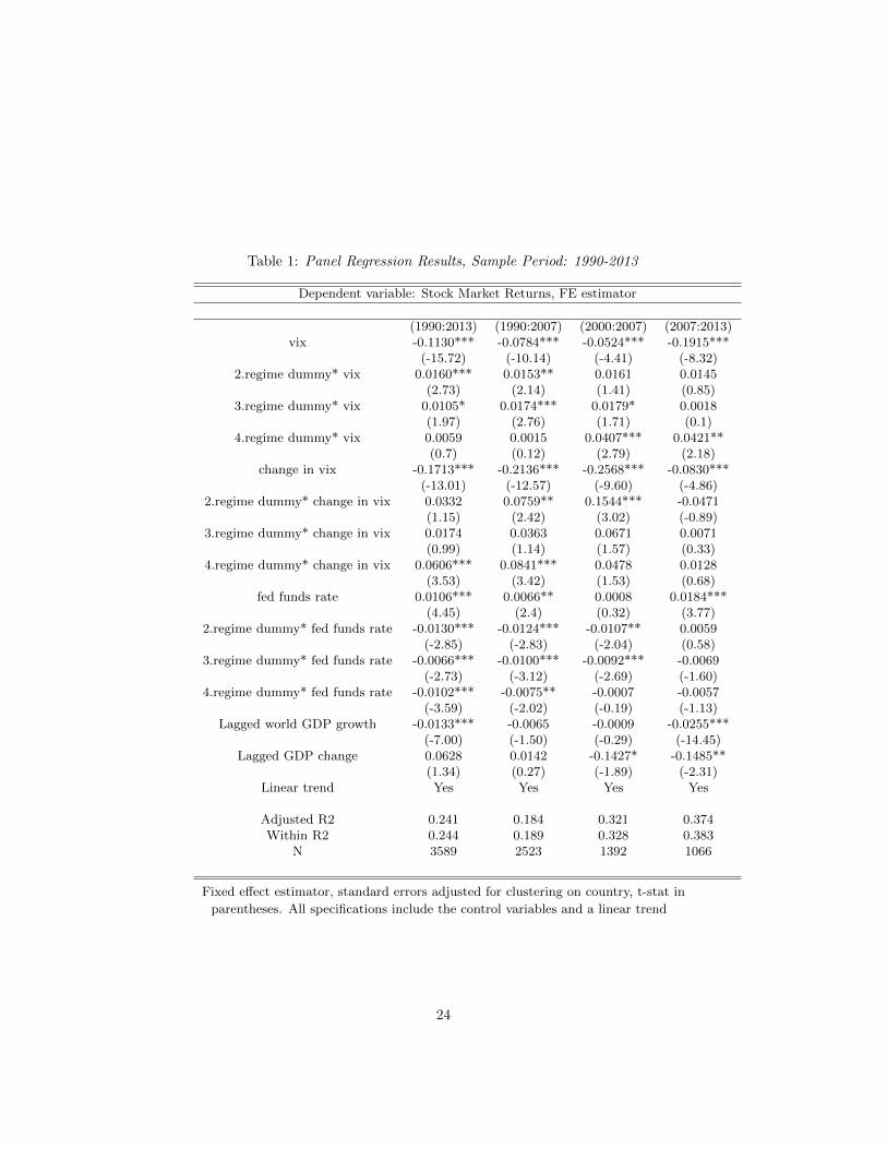
Table 1: Panel Regression Results, Sample Period: 1990-2013
Dependent variable: Stock Market Returns, FE estimator
(1990:2013) (1990:2007) (2000:2007) (2007:2013)vix -0.1130*** -0.0784*** -0.0524*** -0.1915***
(-15.72) (-10.14) (-4.41) (-8.32)2.regime dummy* vix 0.0160*** 0.0153** 0.0161 0.0145
(2.73) (2.14) (1.41) (0.85)3.regime dummy* vix 0.0105* 0.0174*** 0.0179* 0.0018
(1.97) (2.76) (1.71) (0.1)4.regime dummy* vix 0.0059 0.0015 0.0407*** 0.0421**
(0.7) (0.12) (2.79) (2.18)change in vix -0.1713*** -0.2136*** -0.2568*** -0.0830***
(-13.01) (-12.57) (-9.60) (-4.86)2.regime dummy* change in vix 0.0332 0.0759** 0.1544*** -0.0471
(1.15) (2.42) (3.02) (-0.89)3.regime dummy* change in vix 0.0174 0.0363 0.0671 0.0071
(0.99) (1.14) (1.57) (0.33)4.regime dummy* change in vix 0.0606*** 0.0841*** 0.0478 0.0128
(3.53) (3.42) (1.53) (0.68)fed funds rate 0.0106*** 0.0066** 0.0008 0.0184***
(4.45) (2.4) (0.32) (3.77)2.regime dummy* fed funds rate -0.0130*** -0.0124*** -0.0107** 0.0059
(-2.85) (-2.83) (-2.04) (0.58)3.regime dummy* fed funds rate -0.0066*** -0.0100*** -0.0092*** -0.0069
(-2.73) (-3.12) (-2.69) (-1.60)4.regime dummy* fed funds rate -0.0102*** -0.0075** -0.0007 -0.0057
(-3.59) (-2.02) (-0.19) (-1.13)Lagged world GDP growth -0.0133*** -0.0065 -0.0009 -0.0255***
(-7.00) (-1.50) (-0.29) (-14.45)Lagged GDP change 0.0628 0.0142 -0.1427* -0.1485**
(1.34) (0.27) (-1.89) (-2.31)Linear trend Yes Yes Yes Yes
Adjusted R2 0.241 0.184 0.321 0.374Within R2 0.244 0.189 0.328 0.383
N 3589 2523 1392 1066
Fixed effect estimator, standard errors adjusted for clustering on country, t-stat in
parentheses. All specifications include the control variables and a linear trend
24
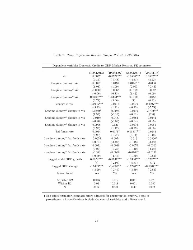
Table 2: Panel Regression Results, Sample Period: 1990-2013
Dependent variable: Domestic Credit to GDP Market Returns, FE estimator
(1990:2013) (1990:2007) (2000:2007) (2007:2013)vix 0.0057 -0.0521*** -0.1508*** 0.1502***
(0.35) (-3.48) (-4.31) (3.22)2.regime dummy* vix 0.0097 0.0139 0.0458** -0.006
(1.01) (1.09) (2.09) (-0.43)3.regime dummy* vix -0.0006 0.0062 0.0199 0.0022
(-0.06) (0.83) (1.42) (0.09)4.regime dummy* vix 0.0208*** 0.0303*** 0.0172 0.0188
(2.72) (3.06) (1) (0.32)change in vix -0.0935*** 0.0417 -0.0079 -0.2997***
(-3.23) (1.21) (-0.23) (-5.78)2.regime dummy* change in vix 0.0840* -0.0085 -0.0419 0.1732***
(1.93) (-0.16) (-0.61) (2.8)3.regime dummy* change in vix -0.0107 -0.0481 -0.0362 0.0442
(-0.26) (-0.86) (-0.64) (0.85)4.regime dummy* change in vix 0.0996 0.127 -0.0576 0.0051
(0.95) (1.17) (-0.79) (0.03)fed funds rate 0.0044 0.0071* 0.0159*** 0.0244
(0.98) (1.77) (3.11) (1.42)2.regime dummy* fed funds rate -0.0053 -0.0074 -0.013 -0.0306*
(-0.84) (-1.20) (-1.48) (-1.99)3.regime dummy* fed funds rate 0.0021 -0.0018 -0.0076 -0.0202
(0.29) (-0.36) (-1.10) (-1.28)4.regime dummy* fed funds rate -0.003 -0.0066 -0.0104* -0.0121
(-0.69) (-1.47) (-1.80) (-0.81)Lagged world GDP growth 0.0074*** -0.0131*** -0.0330*** 0.0267***
(3) (-2.96) (-5.71) -5.72Lagged GDP change -0.5439*** -0.4382** -0.5220*** -0.6007***
(-3.29) (-2.49) (-3.39) (-2.84)Linear trend Yes Yes Yes Yes
Adjusted R2 0.016 0.012 0.041 0.073Within R2 0.02 0.018 0.051 0.085
N 3982 2890 1543 1092
Fixed effect estimator, standard errors adjusted for clustering on country, t-stat in
parentheses. All specifications include the control variables and a linear trend
25
ATBE
BGFR
GRCN
LUN
LCY
PTES
FIIT
IEDK
ECLT
BYSI
ARCR
BOSK
MY
HRDE
RUM
TCZ
THLV
CAHU
ISCH
IDKP
MX
BRGB
PLCL
SECO
NZ
NO
ROTR
AUJP
ZAUS
Aust
ria1.
00Be
lgiu
m0.
421.
00Bu
lgar
ia0.
220.
481.
00Fr
ance
0.43
0.40
0.35
1.00
Gree
ce0.
450.
150.
550.
401.
00Ch
ina:
Hon
g Ko
ng-0
.11
0.36
0.25
0.26
-0.1
91.
00Lu
xem
bour
g0.
210.
420.
150.
48-0
.04
0.59
1.00
Net
herla
nds
0.53
0.46
0.02
0.51
0.06
0.08
0.42
1.00
Cypr
us0.
040.
030.
21-0
.17
0.50
-0.2
8-0
.29
-0.2
31.
00Po
rtug
al0.
450.
140.
330.
380.
54-0
.11
0.01
0.25
0.23
1.00
Spai
n0.
580.
530.
620.
740.
510.
030.
430.
450.
000.
451.
00Fi
nlan
d-0
.16
0.30
0.02
-0.2
5-0
.17
0.27
0.21
-0.1
60.
23-0
.24
-0.0
51.
00Ita
ly0.
620.
210.
050.
530.
180.
090.
430.
56-0
.13
0.36
0.57
-0.0
11.
00Ire
land
0.59
0.42
0.39
0.69
0.36
0.05
0.24
0.46
-0.1
10.
450.
64-0
.28
0.46
1.00
Denm
ark
0.61
0.19
0.33
0.43
0.56
-0.0
90.
070.
440.
110.
460.
39-0
.28
0.47
0.61
1.00
Ecua
dor
0.10
0.06
-0.1
0-0
.08
-0.2
6-0
.03
0.06
0.27
-0.1
8-0
.14
0.00
-0.1
4-0
.12
-0.0
30.
011.
00Lit
huan
ia0.
420.
560.
780.
470.
370.
410.
370.
280.
010.
290.
62-0
.15
0.27
0.61
0.41
-0.0
11.
00Be
laru
s-0
.24
0.03
0.14
-0.2
0-0
.25
0.45
0.38
-0.2
1-0
.15
-0.3
1-0
.14
0.38
-0.1
4-0
.25
-0.1
80.
110.
081.
00Sl
oven
ia0.
550.
510.
520.
630.
500.
140.
400.
50-0
.04
0.35
0.71
-0.0
30.
340.
640.
490.
160.
540.
021.
00Ar
gent
ina
0.19
0.24
0.29
0.26
0.07
0.52
0.54
0.23
-0.0
50.
070.
300.
320.
360.
210.
160.
060.
340.
530.
391.
00Co
sta
Rica
-0.0
80.
330.
510.
04-0
.02
0.44
0.33
-0.0
3-0
.15
-0.3
80.
200.
29-0
.13
0.07
0.10
0.20
0.45
0.48
0.26
0.44
1.00
Boliv
ia-0
.20
0.03
-0.1
9-0
.46
-0.3
30.
11-0
.13
-0.2
4-0
.05
-0.1
4-0
.38
0.19
-0.2
4-0
.38
-0.3
70.
08-0
.18
0.16
-0.3
3-0
.10
-0.1
81.
00Sl
ovak
ia0.
35-0
.01
0.24
0.01
0.44
-0.0
20.
000.
060.
150.
160.
17-0
.11
0.32
-0.0
50.
34-0
.17
0.16
0.08
0.25
0.12
-0.0
50.
211.
00M
alay
sia0.
340.
33-0
.02
0.40
0.01
0.29
0.46
0.49
-0.4
90.
240.
360.
050.
470.
440.
190.
100.
090.
140.
490.
34-0
.02
-0.0
90.
001.
00Cr
oatia
0.14
0.01
0.45
0.35
0.40
-0.0
3-0
.10
-0.2
60.
040.
250.
37-0
.13
-0.1
10.
400.
15-0
.15
0.34
0.05
0.44
0.05
0.06
-0.0
80.
13-0
.05
1.00
Germ
any
0.48
0.64
0.16
0.48
0.12
0.19
0.36
0.69
-0.1
00.
250.
410.
060.
490.
530.
40-0
.10
0.31
-0.2
10.
410.
320.
05-0
.17
-0.0
30.
43-0
.22
1.00
Russ
ia0.
350.
610.
690.
370.
270.
390.
450.
24-0
.10
0.19
0.62
0.16
0.32
0.34
0.24
0.03
0.66
0.34
0.56
0.59
0.50
0.02
0.29
0.32
0.21
0.41
1.00
Mal
ta0.
320.
450.
460.
490.
270.
230.
310.
48-0
.10
0.35
0.56
-0.0
90.
320.
340.
20-0
.03
0.48
-0.0
90.
490.
400.
21-0
.14
0.15
0.37
-0.0
10.
460.
651.
00Cz
ech
Repu
blic
0.05
0.40
0.53
0.19
0.07
0.43
0.23
-0.0
3-0
.20
0.10
0.36
0.16
0.11
0.25
-0.0
1-0
.23
0.49
0.12
0.30
0.33
0.43
0.04
0.05
0.24
0.17
0.15
0.63
0.47
1.00
Thai
land
0.17
0.26
0.08
0.45
-0.0
40.
530.
640.
44-0
.35
0.09
0.23
0.13
0.38
0.18
0.16
0.00
0.15
0.22
0.32
0.61
0.27
-0.0
80.
030.
39-0
.12
0.51
0.27
0.33
0.13
1.00
Latv
ia0.
280.
560.
730.
510.
290.
380.
400.
34-0
.16
0.22
0.65
-0.0
60.
200.
560.
280.
150.
73-0
.04
0.67
0.31
0.50
-0.3
70.
000.
340.
220.
430.
640.
600.
490.
281.
00Ca
nada
0.05
0.06
0.13
0.11
0.09
0.34
0.42
0.13
-0.1
5-0
.06
0.14
0.29
0.13
-0.0
60.
090.
180.
070.
590.
270.
650.
41-0
.14
0.14
0.40
0.02
0.02
0.32
0.29
-0.0
10.
500.
191.
00Hu
ngar
y0.
310.
340.
580.
150.
33-0
.02
-0.0
20.
110.
380.
190.
36-0
.16
-0.0
90.
240.
300.
380.
510.
240.
340.
180.
28-0
.02
0.14
-0.1
60.
310.
020.
370.
22-0
.01
-0.1
10.
320.
171.
00Ice
land
0.49
0.53
0.66
0.65
0.36
0.20
0.39
0.36
0.01
0.35
0.80
-0.1
90.
410.
710.
400.
050.
81-0
.22
0.63
0.20
0.24
-0.3
10.
090.
140.
350.
420.
530.
420.
400.
170.
78-0
.13
0.40
1.00
Switz
erla
nd0.
100.
30-0
.07
0.29
0.09
0.11
0.43
0.41
0.04
-0.0
20.
200.
170.
230.
150.
15-0
.12
0.03
0.08
0.28
0.16
0.00
-0.3
7-0
.06
0.22
-0.1
00.
370.
040.
07-0
.17
0.22
0.13
0.18
-0.0
10.
181.
00In
done
sia-0
.12
-0.0
40.
040.
12-0
.13
0.52
0.46
0.08
-0.3
3-0
.11
-0.0
20.
060.
07-0
.19
-0.0
50.
280.
090.
590.
050.
650.
380.
200.
150.
17-0
.06
0.00
0.41
0.25
0.16
0.56
0.03
0.59
0.05
-0.1
5-0
.13
1.00
Kore
a0.
460.
580.
430.
520.
210.
440.
670.
63-0
.17
0.29
0.52
0.02
0.47
0.51
0.40
0.08
0.55
0.26
0.66
0.52
0.23
-0.2
10.
190.
610.
010.
550.
620.
560.
330.
420.
590.
360.
290.
480.
300.
251.
00M
exico
0.11
0.12
-0.0
20.
17-0
.10
0.27
0.44
0.20
-0.3
3-0
.06
0.06
0.23
0.16
0.04
0.07
0.20
-0.0
60.
500.
380.
580.
270.
060.
170.
440.
030.
220.
390.
330.
070.
530.
130.
64-0
.03
-0.1
10.
170.
590.
401.
00Br
azil
-0.0
10.
330.
150.
16-0
.10
0.61
0.56
0.16
-0.2
6-0
.04
0.10
0.38
0.18
-0.0
6-0
.04
0.03
0.14
0.61
0.21
0.72
0.41
0.08
0.10
0.40
-0.0
90.
360.
600.
300.
330.
630.
210.
62-0
.06
-0.0
60.
100.
760.
450.
591.
00Un
ited
King
dom
0.52
0.50
0.02
0.62
0.12
0.16
0.55
0.75
-0.2
00.
220.
44-0
.18
0.41
0.56
0.36
0.12
0.27
-0.0
90.
510.
26-0
.05
-0.3
4-0
.10
0.47
-0.0
70.
740.
220.
29-0
.12
0.47
0.36
0.12
0.17
0.45
0.65
0.03
0.59
0.27
0.19
1.00
Pola
nd0.
250.
300.
320.
430.
160.
580.
530.
31-0
.33
0.26
0.29
0.10
0.29
0.29
0.29
0.08
0.42
0.47
0.53
0.59
0.28
0.07
0.25
0.49
0.24
0.26
0.52
0.31
0.27
0.65
0.32
0.53
0.13
0.20
-0.0
40.
620.
600.
570.
660.
271.
00Ch
ile-0
.04
0.08
0.08
-0.1
6-0
.25
0.29
0.35
0.12
-0.3
0-0
.14
-0.0
20.
19-0
.04
-0.2
1-0
.05
0.39
0.03
0.64
-0.0
10.
470.
490.
220.
030.
21-0
.18
0.00
0.43
0.21
0.14
0.30
0.03
0.57
0.25
-0.2
3-0
.16
0.72
0.33
0.48
0.62
0.01
0.42
1.00
Swed
en0.
400.
500.
300.
460.
470.
030.
390.
620.
180.
160.
470.
120.
280.
290.
470.
060.
260.
070.
590.
340.
20-0
.33
0.21
0.19
0.07
0.54
0.34
0.24
-0.1
40.
410.
300.
290.
320.
300.
600.
100.
480.
280.
280.
650.
330.
071.
00Co
lom
bia
-0.2
30.
010.
00-0
.09
-0.3
30.
480.
37-0
.11
-0.1
8-0
.46
-0.1
40.
37-0
.06
-0.1
8-0
.12
0.30
0.01
0.67
0.01
0.54
0.58
0.08
0.05
0.01
-0.0
7-0
.08
0.28
-0.1
50.
080.
300.
030.
460.
05-0
.15
-0.0
60.
650.
150.
410.
64-0
.06
0.36
0.63
0.05
1.00
New
Zea
land
0.30
0.59
0.14
0.42
0.11
0.36
0.46
0.52
-0.1
40.
080.
300.
170.
210.
370.
150.
100.
23-0
.04
0.45
0.28
0.20
-0.1
7-0
.07
0.43
-0.0
80.
710.
270.
250.
070.
520.
450.
12-0
.04
0.30
0.27
0.14
0.54
0.25
0.45
0.61
0.37
0.07
0.52
0.15
1.00
Nor
way
0.29
0.45
0.33
0.29
0.17
0.18
0.14
0.28
0.19
0.11
0.32
0.31
0.09
0.32
0.21
0.05
0.35
-0.2
00.
500.
250.
28-0
.30
-0.1
6-0
.02
0.15
0.39
0.14
0.23
0.12
0.36
0.49
0.07
0.17
0.47
0.27
-0.2
20.
180.
04-0
.01
0.30
0.17
-0.2
60.
40-0
.08
0.32
1.00
Rom
ania
0.37
0.44
0.81
0.52
0.51
0.32
0.28
0.25
0.05
0.33
0.64
-0.1
50.
150.
510.
350.
140.
830.
040.
650.
410.
42-0
.20
0.18
0.13
0.43
0.23
0.68
0.60
0.48
0.25
0.78
0.21
0.53
0.71
-0.1
10.
260.
480.
140.
210.
190.
500.
070.
310.
010.
250.
381.
00Tu
rkey
0.26
0.55
0.45
0.45
0.01
0.47
0.60
0.41
-0.2
50.
040.
560.
290.
400.
320.
100.
060.
530.
290.
480.
730.
55-0
.16
0.00
0.34
0.00
0.47
0.78
0.66
0.56
0.58
0.57
0.41
0.12
0.43
0.11
0.52
0.56
0.46
0.66
0.31
0.56
0.42
0.35
0.39
0.39
0.35
0.59
1.00
Aust
ralia
-0.0
80.
280.
290.
300.
180.
440.
360.
100.
010.
060.
220.
350.
010.
02-0
.07
-0.1
20.
080.
280.
250.
410.
31-0
.11
0.07
0.26
0.13
0.23
0.36
0.35
0.16
0.45
0.29
0.49
-0.0
5-0
.04
0.03
0.43
0.36
0.36
0.66
0.09
0.41
0.36
0.32
0.42
0.53
0.09
0.23
0.43
1.00
Japa
n0.
090.
36-0
.07
0.18
-0.3
30.
390.
420.
40-0
.32
-0.1
50.
060.
090.
170.
29-0
.03
0.04
0.21
0.18
0.28
0.36
0.16
0.14
-0.0
50.
29-0
.09
0.41
0.29
0.14
0.32
0.33
0.15
-0.0
2-0
.05
0.19
0.23
0.21
0.41
0.23
0.32
0.47
0.32
0.26
0.18
0.36
0.26
0.21
0.03
0.42
0.04
1.00
Sout
h Af
rica
0.38
0.19
0.26
0.42
0.15
0.31
0.56
0.49
-0.3
20.
310.
42-0
.15
0.43
0.36
0.25
0.05
0.30
0.13
0.31
0.55
0.14
-0.1
70.
120.
48-0
.02
0.41
0.43
0.55
0.22
0.58
0.39
0.47
0.09
0.28
0.18
0.44
0.63
0.42
0.42
0.50
0.39
0.45
0.30
0.11
0.34
-0.0
20.
350.
490.
410.
241.
00Un
ited
Stat
es0.
400.
430.
140.
67-0
.07
0.36
0.56
0.64
-0.3
60.
170.
53-0
.11
0.41
0.59
0.25
0.24
0.38
0.06
0.61
0.41
0.15
-0.3
8-0
.15
0.55
0.17
0.56
0.30
0.33
0.08
0.60
0.53
0.29
0.18
0.54
0.42
0.16
0.57
0.30
0.32
0.75
0.45
0.08
0.44
0.13
0.50
0.47
0.35
0.49
0.24
0.50
0.48
1.00
Figure 5: Heatmap of correlations of gross inflows across countries classified bycurrency regimes, 1990-2012
26
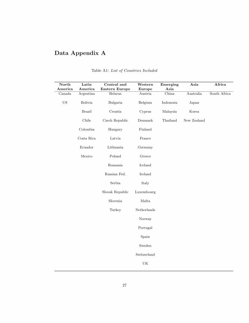
Data Appendix A
Table A1: List of Countries Included
North Latin Central and Western Emerging Asia AfricaAmerica America Eastern Europe Europe Asia
Canada Argentina Belarus Austria China Australia South Africa
US Bolivia Bulgaria Belgium Indonesia Japan
Brazil Croatia Cyprus Malaysia Korea
Chile Czech Republic Denmark Thailand New Zealand
Colombia Hungary Finland
Costa Rica Latvia France
Ecuador Lithuania Germany
Mexico Poland Greece
Romania Iceland
Russian Fed. Ireland
Serbia Italy
Slovak Republic Luxembourg
Slovenia Malta
Turkey Netherlands
Norway
Portugal
Spain
Sweden
Switzerland
UK
27
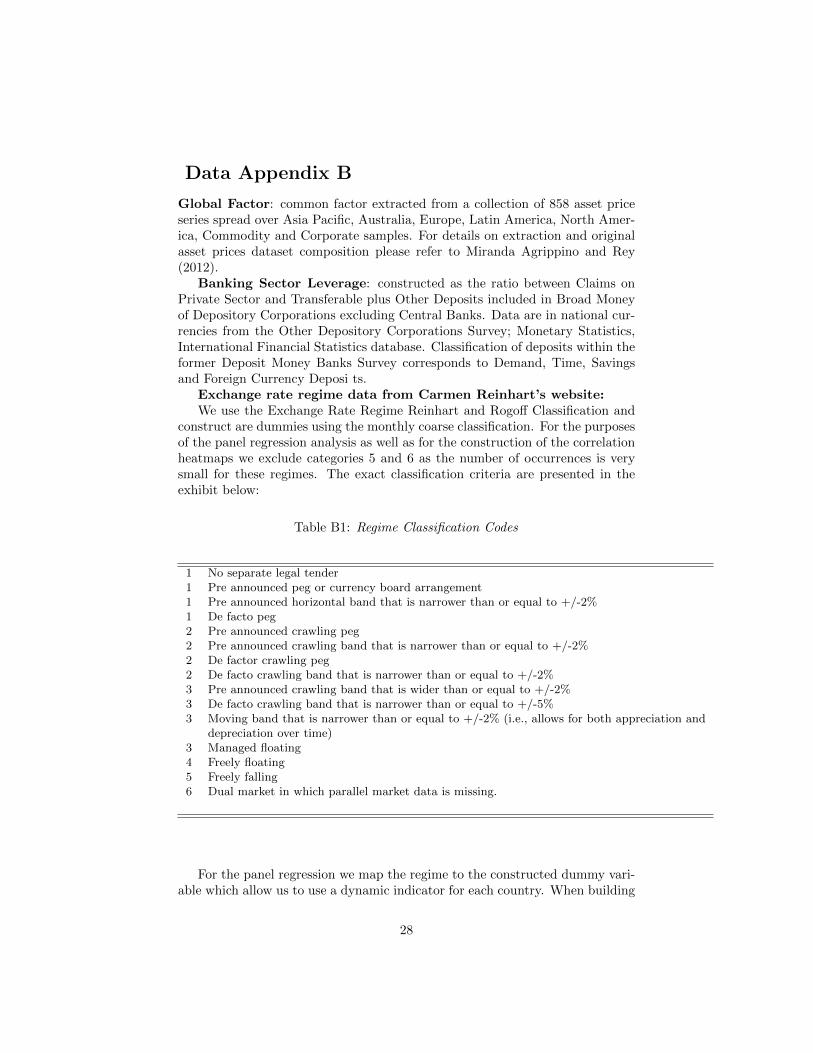
Data Appendix B
Global Factor: common factor extracted from a collection of 858 asset priceseries spread over Asia Pacific, Australia, Europe, Latin America, North Amer-ica, Commodity and Corporate samples. For details on extraction and originalasset prices dataset composition please refer to Miranda Agrippino and Rey(2012).
Banking Sector Leverage: constructed as the ratio between Claims onPrivate Sector and Transferable plus Other Deposits included in Broad Moneyof Depository Corporations excluding Central Banks. Data are in national cur-rencies from the Other Depository Corporations Survey; Monetary Statistics,International Financial Statistics database. Classification of deposits within theformer Deposit Money Banks Survey corresponds to Demand, Time, Savingsand Foreign Currency Deposi ts.
Exchange rate regime data from Carmen Reinhart’s website:We use the Exchange Rate Regime Reinhart and Rogoff Classification and
construct are dummies using the monthly coarse classification. For the purposesof the panel regression analysis as well as for the construction of the correlationheatmaps we exclude categories 5 and 6 as the number of occurrences is verysmall for these regimes. The exact classification criteria are presented in theexhibit below:
Table B1: Regime Classification Codes
1 No separate legal tender1 Pre announced peg or currency board arrangement1 Pre announced horizontal band that is narrower than or equal to +/-2%1 De facto peg2 Pre announced crawling peg2 Pre announced crawling band that is narrower than or equal to +/-2%2 De factor crawling peg2 De facto crawling band that is narrower than or equal to +/-2%3 Pre announced crawling band that is wider than or equal to +/-2%3 De facto crawling band that is narrower than or equal to +/-5%3 Moving band that is narrower than or equal to +/-2% (i.e., allows for both appreciation and
depreciation over time)3 Managed floating4 Freely floating5 Freely falling6 Dual market in which parallel market data is missing.
For the panel regression we map the regime to the constructed dummy vari-able which allow us to use a dynamic indicator for each country. When building
28
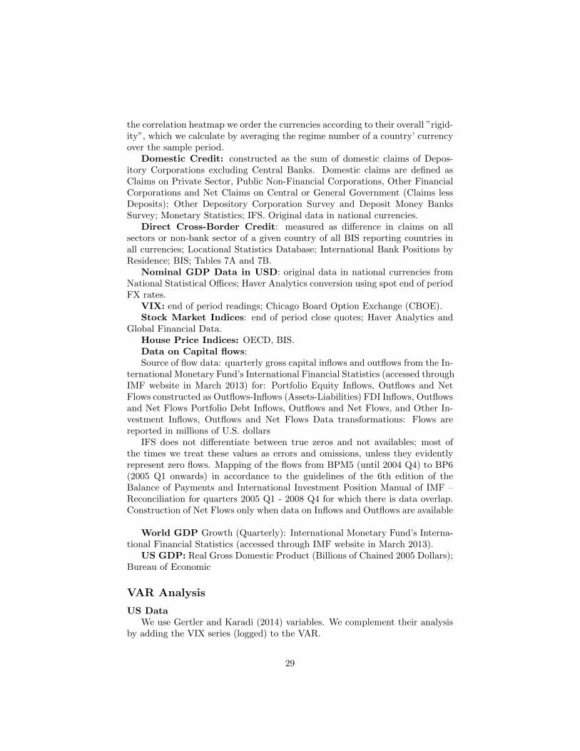
the correlation heatmap we order the currencies according to their overall ”rigid-ity”, which we calculate by averaging the regime number of a country’ currencyover the sample period.
Domestic Credit: constructed as the sum of domestic claims of Depos-itory Corporations excluding Central Banks. Domestic claims are defined asClaims on Private Sector, Public Non-Financial Corporations, Other FinancialCorporations and Net Claims on Central or General Government (Claims lessDeposits); Other Depository Corporation Survey and Deposit Money BanksSurvey; Monetary Statistics; IFS. Original data in national currencies.
Direct Cross-Border Credit: measured as difference in claims on allsectors or non-bank sector of a given country of all BIS reporting countries inall currencies; Locational Statistics Database; International Bank Positions byResidence; BIS; Tables 7A and 7B.
Nominal GDP Data in USD: original data in national currencies fromNational Statistical Offices; Haver Analytics conversion using spot end of periodFX rates.
VIX: end of period readings; Chicago Board Option Exchange (CBOE).Stock Market Indices: end of period close quotes; Haver Analytics and
Global Financial Data.House Price Indices: OECD, BIS.Data on Capital flows:Source of flow data: quarterly gross capital inflows and outflows from the In-
ternational Monetary Fund’s International Financial Statistics (accessed throughIMF website in March 2013) for: Portfolio Equity Inflows, Outflows and NetFlows constructed as Outflows-Inflows (Assets-Liabilities) FDI Inflows, Outflowsand Net Flows Portfolio Debt Inflows, Outflows and Net Flows, and Other In-vestment Inflows, Outflows and Net Flows Data transformations: Flows arereported in millions of U.S. dollars
IFS does not differentiate between true zeros and not availables; most ofthe times we treat these values as errors and omissions, unless they evidentlyrepresent zero flows. Mapping of the flows from BPM5 (until 2004 Q4) to BP6(2005 Q1 onwards) in accordance to the guidelines of the 6th edition of theBalance of Payments and International Investment Position Manual of IMF –Reconciliation for quarters 2005 Q1 - 2008 Q4 for which there is data overlap.Construction of Net Flows only when data on Inflows and Outflows are available
World GDP Growth (Quarterly): International Monetary Fund’s Interna-tional Financial Statistics (accessed through IMF website in March 2013).
US GDP: Real Gross Domestic Product (Billions of Chained 2005 Dollars);Bureau of Economic
VAR Analysis
US DataWe use Gertler and Karadi (2014) variables. We complement their analysis
by adding the VIX series (logged) to the VAR.
29
UK DataFor the data used in the UK VAR spanning a period between 1995 and 2014,
we additionally employ: -Monthly CPI data and monthly industrial productiondata (seasonally adjusted) from the IMF (IFS database). -A constructed mort-gage spread series using monthly data from the Bank of England. The mortgagespread is calculated as the difference of the Bank Rate Tracker (series bv24)(extended further back with the Standard Variable Rate) from the 3M LIBOR.-The UK policy rate calculated as a monthly average of the Official Bank ratefrom the Bank of England.
30