Finance and Economics Discussion SeriesDivisions of Research & Statistics and Monetary Affairs

Federal Reserve Board, Washington, D.C.

Mutual Fund Flows, Monetary Policy and Financial Stability

Ayelen Banegas, Gabriel Montes-Rojas, and Lucas Siga

2016-071

Please cite this paper as:Banegas, Ayelen, and Gabriel Montes-Rojas, Lucas Siga (2016). “Mutual FundFlows, Monetary Policy and Financial Stability,” Finance and Economics DiscussionSeries 2016-071. Washington: Board of Governors of the Federal Reserve System,http://dx.doi.org/10.17016/FEDS.2016.071.

NOTE: Staff working papers in the Finance and Economics Discussion Series (FEDS) are preliminarymaterials circulated to stimulate discussion and critical comment. The analysis and conclusions set forthare those of the authors and do not indicate concurrence by other members of the research staff or theBoard of Governors. References in publications to the Finance and Economics Discussion Series (other thanacknowledgement) should be cleared with the author(s) to protect the tentative character of these papers.

Mutual Fund Flows, Monetary Policy and Financial

Stability∗

Ayelen Banegas†, Gabriel Montes-Rojas‡, Lucas Siga§

July 26, 2016

Abstract

We study the links between monetary policy and mutual fund flows, and the po-tential risks to financial stability that might arise from such flows, using data over the2000–14 period. We find that monetary policy can have a direct influence on the allo-cation decisions of mutual fund investors. In particular, we show that monetary policyshocks explain mutual fund flow dynamics and that the effect of these shocks differs byinvestment strategy. Results suggest that positive shocks to the path of monetary pol-icy (unexpected tightening) are associated with persistent outflows from bond mutualfunds. Conversely, a tighter-than-expected monetary policy path will cause net inflowsinto equity funds. In an industry that “mutualizes” redemption costs and where manyfunds may engage in liquidity transformation, our flow-performance analysis providesevidence of the potential existence of a first-mover advantage in less liquid segments ofthe market.

Keywords: Mutual fund flows, monetary policy, first-mover advantageJEL Classification: G20, G23, E52

∗The views expressed in this paper are solely the responsibility of the authors and should not be interpretedas reflecting the views of the Board of Governors of the Federal Reserve System.†Federal Reserve Board, Division of Monetary Affairs. Email: maria.a.banegas@frb.gov‡CONICET-Universidad de San Andres. Email: gmontesrojas@udesa.edu.ar§New York University – Abu Dahbi. Email: lucas.siga@nyu.edu

1

1 Introduction

In response to the recent crisis that emerged during the summer of 2007, the Federal Re-

serve has been actively implementing policies to support economic growth by lowering yields

across the curve and making financial conditions more accommodative. For instance, imme-

diately after the burst of the crisis, the Fed launched a series of credit and liquidity facilities

and began aggressively cutting the fed funds target rate, reaching the zero lower bound by

the end of 2008. Thereafter, the Fed turned to unconventional policy tools to provide addi-

tional downward pressure on longer-term interest rates. These tools included a series of asset

purchase programs (quantitative easing), a maturity extension program, and a more active

communication strategy involving forward guidance about the future path of the federal

funds rate (FFR).1 In particular, the Fed’s asset purchase programs were intended to work

largely through the portfolio balance channel by reducing longer-term rates and term pre-

miums, therefore creating more favorable financial conditions such as lower financing costs

for firms and households.

As bond yields declined and the stock market recovered in the United States, the bond

market surged by 41 percent and equity markets rose by 112 percent during the period

from October 2008 to the end of 2014. In this context, the U.S. mutual fund industry saw

massive inflows in the years following the onset of the financial crisis, with net new cash

flows into long-term mutual funds reaching $1.1 trillion by the end of 2014 and total assets

under management increasing to $13 trillion, an additional $7.4 trillion relative to the level

observed at the end of 2008.2

This dramatic growth in assets under management, together with the recent selloff

1Several studies review the programs implemented by the Fed during the past years. See Engen, Laubach,and Reifschneider (2015) for more details.

2Long-term mutual funds refer to funds investing in either equity, bond or hybrid funds as defined bythe Investment Company Institute (ICI). These statistics exclude mutual funds investing in money markets.Including money market mutual funds, total net assets reached $15.8 trillion by the end of 2014.

2

episodes that took place in 2013 and 2014, brought mutual funds to the center of the debate

on the potential disruptions to financial markets that might arise from the mutual fund in-

dustry once the Fed normalizes the stance of monetary policy. In particular, there is concern

among policymakers and some market participants about how mutual fund investors and

asset managers will respond to monetary policy normalization and, ultimately, the effect of

their behavior on household wealth and financial stability.

Specific to fund investors, the debate has focused on the risks to run-like dynamics and,

therefore, whether mutual fund flows could be an important source of financial instability if

an event, potentially the rise in interest rates, were to trigger large redemptions from mutual

funds that could result in disruptions in the underlying asset markets.3 In particular, the

recent “taper tantrum” in 2013 and the emerging markets selloff in 2014 centered the debate

primarily on bond mutual funds and the potential implications for financial stability of

massive redemptions affecting less liquid segments of the bond market.

By offering investors the possibility of daily redemption of their shares, mutual funds

investing in illiquid assets engage in liquidity transformation and may face liquidity risk in

the event investors massively redeem shares of their funds. In this scenario, as fund managers

need to liquidate less liquid positions to meet redemptions, they might generate downward

price pressure on the underlying assets, which in turn decreases the value of the fund’s shares.

In other words, in the case that massive redemptions create disruptions in the underlying

assets of the fund, the cost will be borne by those who remained invested in the fund. In

an extreme scenario, this “mutualization” of redemption costs could potentially lead to fire

sales, as investors will have economic incentives to redeem ahead of the anticipated outflows,

also referred to as “first-mover advantage.”4

3See the Monetary Policy Report submitted to the Congress by the Federal Reserve in February 2015(www.federalreserve.gov/monetarypolicy/files/20150224 mprfullreport.pdf).

4This concept has been largely study in the literature on bank runs.

3

From the fund manager side, key questions relate to how asset managers are positioning

their portfolios for interest rate hikes, more stringent liquidity conditions, and more volatile

rate environments, as well as whether they have liquidity strategies in place that will allow

them to manage large and sudden redemptions without creating or amplifying disruptions

in financial markets.5

In this paper, we focus on fund investors and build on the mutual fund literature on

the flow-performance relationship and on the macro-finance literature on monetary policy

and asset prices to shed some light on the effect of monetary policy on investors’ allocation

decisions, as evidenced by mutual fund flows, and the risks to financial stability that fund

investors might create. More specifically, using a unified framework that allows us to study

the effect of monetary policy on fund flows and the flow impact on fund performance, we ask

whether monetary policy shocks in the United States can help explain aggregate fund flows

across different asset classes and investment styles, and whether these flows can generate

negative price effects that could trigger run-like dynamics in the mutual fund industry. Intu-

itively, because monetary policy is ultimately expected to affect economic growth, changes in

investors’ expectations about the stance of monetary policy can be expected to have a direct

effect on investors’ portfolio allocations and, therefore, related fund flows. Although in recent

years there has been a vast body of work on the response of asset prices around monetary

policy announcements, the study of the effects of monetary policy on investment vehicles

such as mutual funds remains a largely unexplored area of research.6 We also evaluate the

5Reportedly, fixed-income managers have been improving their liquidity management practices in recentyears. For example, funds may try to manage liquidity through internal portfolio construction by holding alarger share of their portfolios on highly liquid assets, managing liquidity at the firm level, or expanding theircredit lines, among other tools. Furthermore, the Securities and Exchange Commission recently proposed anew rule on liquidity management affecting open-end mutual funds that includes the development of liquidityrisk-management programs, the need for liquidity buffers, classification of portfolio holdings based on thelevel of liquidity of the position, and the possibility of implementing swing pricing.

6There is a large literature on the effects of monetary policy on asset prices using high-frequency datain the context of event studies to avoid the widely known omitted variables and endogeneity issues. Thesestudies include Kuttner (2001); Bernanke and Kuttner (2005); Gurkaynak, Sack, and Swanson (2005); and

4

relation between macroeconomic and financial conditions and the investment behavior of

mutual fund investors. To this end, we analyze whether mutual fund flows react to infor-

mation on macroeconomic fundamentals and financial conditions as summarized by market

volatility, consumer sentiment, liquidity, the term spread, financial market returns, inflation,

economic activity measures, and changes in the size of the Fed’s balance sheet.

The second part of this paper evaluates the price effect of fund flows on performance

and its implication for run-like behavior. Our analysis is related to recent studies that find

mixed results about the existence of a first-mover advantage. For instance, using a recursive

vector autoregression (VAR), Feroli, Kashyap, Schoenholtz, and Shin (2014) find evidence

of what they define as a “feedback loop” between flows and returns in some fund categories

such as emerging market bonds, mortgage-backed securities (MBS), and investment-grade

bonds; they argue that financial stability risks can arise from unlevered fund managers.

In contrast, Plantier and Collins (2014) find little evidence of a feedback effect from fund

flows to fund returns (bond prices) when altering the order of the endogenous variables in

a recursive VAR model. More recently, and focusing on corporate bond funds, Goldstein,

Jiang, and Ng (2015) show that fund flows are more sensitive to poor performance than good

performance and that this relationship is stronger when market liquidity is limited. They

argue that an illiquid corporate bond market may generate a first-mover advantage in mutual

funds investing in this segment of the market. Chen, Goldstein, and Jiang (2010) introduce

a global-game model that formalizes the mechanisms through which large and sudden re-

demptions from illiquid funds can effectively transform into costs faced by those investors

who remained invested in the fund. This mechanism implies strategic complementarities in

Lucca and Moench (2015). More recently, many papers have focused on the effects of the Feds quantitativeprograms on asset prices, including Gagnon, Raskin, Remache, and Sack (2011); Hamilton and Wu (2012);Rosa (2012); DAmico, English, Salido, and Nelson (2012); DAmico and King (2013); and Rogers, Scotti,and Wright (2014), among others.

5

the redemption decisionmaking that can lead to run-like behavior.7 They provide evidence

of this effect by analyzing equity funds for the 1995-2005 period. In this setting, our findings

can be interpreted as a quantitative assessment of the risk that monetary policy may have

on triggering this type of mechanism.

A critical aspect of our analysis is the measurement of monetary policy shocks. In

a period characterized by unconventional monetary policy actions, there is no consensus

about the optimal approach to measuring monetary policy shocks. We thus take an agnostic

approach and evaluate a set of alternative measures, including target and path shock factors.

First, we follow Christiano, Eichenbaum, and Evans (1996) (CEE hereafter), who propose to

measure exogenous monetary shocks using orthogonalized shocks to the FFR in a structural

VAR model. Second, we build a proxy of policy shocks using federal funds futures data to

construct a measure of “surprise” target rate changes as proposed by Bernanke and Kuttner

(2005) (BK hereafter). Although these two measures have been widely used in the empirical

macro-finance literature, they fail to fully capture shocks to monetary policy that arise from

tools other than the policy rate. This limitation is an important issue in our analysis because

a large part of our sample covers the zero lower bound, a period during which the Fed has

been actively implementing monetary policy through unconventional policy tools. To address

this issue, we build a third proxy for monetary shocks using monthly data from the Blue

Chip Financial Forecasts (BCFF) and the Blue Chip Economic Indicators (BCEI) surveys

as introduced by Buraschi, Carnelli, and Whelan (2014) (BCW hereafter). More specifically,

we identify the shocks through a Taylor rule using survey data on expectations about future

GDP growth, inflation, and the FFR. Intuitively, by using this approach, we intend to

capture shocks to the path of monetary policy. For example, this monetary shock measure

7Using a similar global-game modeling approach, Feroli, Kashyap, Schoenholtz, and Shin (2014) proposean alternative destabilization channel for mutual funds. In their framework, the strategic asset managersare averse to being ranked last, and, in certain economic environments, this motive may lead to large assetsales.

6

reflects the surprises about future policy that can be inferred from forward guidance or

other communications by Board members. Interestingly, and as in BCW, we find a negative

correlation between target and path shocks. BK and CEE shocks tend to be pro-cyclical,

and BCW path shocks are countercyclical. BCW argue that these patterns are consistent

with a yield curve with a pro-cyclical short-end and a countercyclical long-end, with the

former driven by target shocks and the latter related to path shocks, which BCW find to

be correlated to risk premiums. We argue that BCW shocks are better suited to capture

unexpected shocks to monetary policy in a dynamic and changing environment in which the

Fed has intervened with different tools.

Using a structural VAR identification strategy and ICI data on mutual fund flows and

total net assets aggregated by investment strategy, we find that monetary policy shocks, past

fund returns, and a set of macroeconomic and financial aggregates can help explain mutual

fund flow dynamics and that drivers of flows differ by investment strategy. Interestingly,

we find a clear asymmetry in the effect of these shocks on mutual funds flows. That is, a

positive target shock corresponds to a negative path shock in terms of its effect on mutual

funds flows, and this finding is robust across different mutual fund strategies. Given our

analysis of target versus path monetary shocks, we conclude that the BCW method provides

a more suitable picture of the effect of monetary policy on mutual fund flows and, therefore,

we build our economic interpretation on path shocks.

More specifically, for the bond market, results show that a tightening of monetary policy

(that is, a positive target shock) will translate into a 0.4 to 0.5 standard deviation increase

in the flow-to-assets ratio, and a positive path shock will produce outflows on the order of

0.8 standard deviation. Within the bond fund universe, results are mainly driven by the

taxable bond segment of the market, including government, high-yield, investment-grade,

multisector, and world bond funds. For equity, the effect of monetary path shocks on flow of

7

funds investing in equity markets is negative for target shocks (0.2 to 0.4 standard deviation)

and positive for path shocks (0.5 standard deviation). Thus, these findings are consistent

with the argument that as the economy improves, investors will shift their portfolio alloca-

tions from safe-haven to riskier assets. Furthermore, although flow of funds investing in the

government, municipal, investment-grade, and multisector bond markets exhibit a counter-

cyclical relationship with macro conditions, high-yield bond flows show a cyclical pattern,

similar to equity flows. Interestingly , we document strong co-movements between high-yield

and equity fund flows throughout the analysis.

In turn, our flow-performance analysis shows that outflows can have an effect on the

performance of funds investing in bonds and in less liquid segments of the equity market. As a

result, under the current regulatory framework in which redemption costs are mutualized and

mutual funds engage in liquidity transformation, our findings suggest that there are economic

incentives that may generate a first-mover advantage. However, we argue that adequate

liquidity-management practices and policy guidelines can help mitigate these incentives.

In summary, the main contributions of this paper to the mutual fund literature are

twofold. First, we document that monetary policy has a direct influence on the behavior of

mutual fund investors. Specifically, our results show that positive monetary policy shocks

(tightening) can trigger outflows in funds investing in fixed-income securities and inflows into

international equity funds. Second, we evaluate the price effect of fund flows on performance

and its implication for run-like behavior. We show that mutual fund investors may have

economic incentives that can generate a first-mover advantage in funds investing in less

liquid asset classes.

The paper is organized as follows. Section 2 describes the ICI mutual fund data, monetary

policy shocks, and macroeconomic and financial factors used in our analysis. Section 3

discusses the empirical methodology. Section 4 presents our empirical findings. Section 5

8

concludes.

2 Data and monetary policy shocks estimation

2.1 Mutual funds

We use monthly data on net new flows and total net assets on the 51 ICI investment categories

on long-term mutual funds (namely bond, equity, and hybrid funds) domiciled in the United

States over the 2000–14 period.8 Our flow data account for dividends and income gains to

correctly identify new money in an investment strategy. Specifically, ICI calculates flows for

each investment category as follows:

ft = st − ret + et − dt, (1)

where ft is net new cash flows during month t, st is total sales, ret accounts for monthly

redemptions, et stands for net exchanges, defined as the dollar amount of net shareholder

switches into or out of funds in the same complex during month t, and dt is all reinvested

dividends during the current month.9

Key to the analysis of flow dynamics is understanding who holds mutual fund shares

(retail versus institutional investors), where these funds are invested, and how sticky these

investments are expected to be. In this section, we describe our mutual fund data set to

address some of these questions.

As shown in table 1, after declining by about 35 percent in 2008, U.S. long-term mutual

fund assets have grown dramatically, with total net assets increasing from $5.7 trillion to

8Our decision to use aggregated data at the investment strategy level is motivated by our interest instudying the effect of mutual fund flows on financial markets and the potential implications for financialstability, rather than the specific feedback effects of particular funds that might cancel out at the aggregatelevel.

9Although many asset managers treat reinvested dividends as new cash, ICI excludes them from estimatedflows, as in these cases investors are not consciously making a decision to buy more shares of the fund.

9

$13.1 trillion by the end of 2014. Equity mutual funds experienced the largest increases as

underlying markets recovered, jumping from $3.6 trillion to $8.3 trillion. Similarly, total

assets of bond funds more than doubled over the same period, reaching $3.4 trillion by

the end of 2014. Within the bond segment, funds investing in investment-grade instruments

account for the largest share of the universe at $1.5 trillion; high-yield and world bond funds,

which experienced the largest growth rates during the 2008–14 period, reached close to $0.4

trillion and $0.5 trillion, respectively, by the end of 2014. Conversely, money market mutual

fund assets, not shown, contracted around 30 percent over the same period. This asset

class was particularly hurt by the prolonged low interest rate environment that compressed

returns in money markets.

In terms of long-term mutual fund ownership, individuals are the largest investors, hold-

ing about 92 percent of the assets, and institutional investors account for the remaining 8

percent. Note that these shares moved in a very tight range over the sample period.10 Within

asset classes, although institutional investors share of total assets was steady throughout the

sample period at around 10 percent for bond funds, their share of total assets in equity funds

increased from 5 percent to 8 percent over the same period. In turn, as shown in panel C of

table 1, about 46 percent of total assets are retirement-related assets, which are sometimes

referred to as “sticky assets,” as they tend to be stable long-term investment allocations.

Furthermore, retirement accounts are expected to receive periodic and stable inflows from

investors payrolls and tend to be less reactive to changes in market conditions than nonre-

tirement assets. This fact is important when analyzing flow dynamics and the potential risk

for run-like behavior in the mutual fund industry.

As shown in panel D of table 1, ICI data indicate that the level of concentration in

the mutual fund industry has remained stable over time, with the largest five complexes

10Conversely, the share of institutional investors in money market funds is significantly larger than inlong-term funds, at about 40 percent.

10

accounting for about 40 percent of total assets.

[INSERT TABLE 1 HERE]

In terms of flows, bond mutual funds experienced the largest net inflows over the sample

period. In particular, as shown in figures 1 and 3, bond funds saw massive post-crisis inflows,

with net new cash flows close to $1 trillion for the 2009 –14 period. Furthermore, as presented

in figure 2,inflows into investment-grade bond funds reached close to $384 billion over the

post-crisis period, followed by world bond funds at $186 billion and multisector bond funds

at $195 billion. Meanwhile, inflows into funds investing in high-yield bonds reached $109

billion over the same period. Table 2 presents summary statistics for the broader mutual

fund categories (equity, bond, and hybrid funds) and selected equity and bond categories.

As shown in panels B and C of table 2, volatility of flows increased significantly from the pre-

to post-crisis periods across investment categories. This increase in volatility is particularly

remarkable for bond mutual funds, where monthly volatility jumped from $7.9 billion in

the earlier part of the sample to $20 billion in the post-crisis period. As presented in

table 2,these jumps in flow volatility were significant across bond investment categories.

Similarly, volatility in hybrid flows rose from $2.7 billion to $4.6 billion over the same period.

Meanwhile, volatility of total equity flows was little changed at about $17 billion.

[INSERT FIGURE 1 HERE]

[INSERT FIGURE 3 HERE]

[INSERT FIGURE 2 HERE]

[INSERT TABLE 2 HERE]

As described in table 3, flow correlations changed significantly over the sample period for

some asset classes. For instance, the negative correlation between total equity and bond

flows reverted from close to negative 0.5 in the pre-crisis period to 0.1 in the post-crisis

years. Interestingly, this change in correlations of new mutual fund cash flows is similar

11

to the changes in correlations observed in the returns of the underlying equity and bond

markets. Correlation between flows into equity and hybrid funds rose from 0.1 to 0.7, and

that of equity and high-yield flows doubled to around 0.4. In particular, correlation of

high-yield and domestic equities increased from 0.2 to 0.5 over the two sample periods.

[INSERT TABLE 3 HERE]

We also use data on total net assets to estimate price returns as follows:

rt =at − fit − at−1

at−1

, (2)

where rt is monthly price returns, at is total net assets at the end of month t, and fit

is total net flows including distributions. Table 4 presents performance statistics for the

different investment categories. Similar to the patterns observed in mutual fund flows, return

volatility increased in the post-crisis relative to the pre-crisis period for equity, hybrid, and

bond mutual funds. Within equity funds, the increase in volatility of emerging market equity

funds was remarkable (from 5.6 to 8.5 percent) over the period. In bond markets, volatility

rose consistently across categories, with high yield funds experiencing the largest increase

(from 1.9 percent in the pre-crisis to 4.8 percent in the post-crisis period). Figure 4 plots

monthly returns for our main mutual fund aggregates.

[INSERT FIGURE 4 HERE]

[INSERT TABLE 4 HERE]

Return correlations of equities and bond funds increased at the broader asset class level

over the sample period. At the investment strategy level, as shown in panels A and B of

table 5, return correlations of investment-grade and government funds decreased significantly

from 0.85 to 0.37, while correlation of investment-grade and high yield funds rose from 0.25

to 0.66 over the period. Meanwhile, correlations of equity categories did not change much.

[INSERT TABLE 5 HERE]

12

2.2 Macroeconomic and financial factors

Investors are expected to factor in changes in macroeconomic and financial conditions when

deciding on their investment allocations. For instance, information about the economy is

likely to influence their expectations about future corporate earnings and therefore expected

equity returns. More broadly, investors’ risk appetite is expected to be shaped by the eco-

nomic outlook. To account for these elements, we build macroeconomic factors using princi-

pal component analysis to summarize the information of a large set of economic indicators.

We include series for industrial production, retail sales, housing indicators, IS manufacturing

survey indicators (new orders, inventories, and export orders), and consumer surveys (cur-

rent conditions, consumer sentiment, and expected labor conditions). Time series for these

macro factors are shown in figure 5. We also consider a series for inflation, as measured by

the consumer price index, and a set of financial variables. These variables include equity

market volatility (VIX), the term spread, changes in the size of the Federal Reserve’s balance

sheet, global bond index returns, and returns for the S&P 500 index.

[INSERT FIGURE 5 HERE]

2.3 Monetary policy shocks

Financial and nonfinancial markets are unlikely to respond to policy actions that were already

anticipated. That is, if the Fed’s actions are systematically related to economic variables

(such as inflation or the output gap) that are observed by the Fed and economic agents,

then the anticipatory responses occur before the actual change happens (such as a tight-

ening of monetary policy or increment of the interest rate). In those cases, it is difficult

to identify the causal effect of monetary policy on financial markets. Distinguishing thus

between expected and unexpected policy actions has been a key fundamental challenge in

the literature and, as a result, the definition of a shock and how it is constructed varies. We

13

follow a skeptical approach and construct different measures of monetary shocks. As argued

later, these measures differ not only on the identifying assumptions, but also on what type

of shock they are intended to capture.

First, we consider the orthogonalized shocks from a VAR model with identifying restric-

tions. Since Bernanke and Blinder (1992) and Sims (1992), a considerable literature has

employed VAR methods to identify and measure these shocks. The canonical methodology

that we follow is that of CEE, who propose to measure exogenous monetary shocks using

orthogonalized shocks to the FFR in a structural VAR model. The system is identified by

assuming that Fed behavior has no contemporary effect on other “real” economic variables

but takes them into account for policy actions.

Second, we construct shocks as in BK, who follow Kuttner (2001) in using FFR futures

data to construct a measure of “surprise” rate changes. They use the event-study analysis

of comparing the one-month future contract with the actual target rate set by the Fed. The

economic rationale is that future interest rates reflect expectations about monetary policies,

and, thus, deviations of the actual rate from the predicted one by the futures market represent

a shock. Their approach overcomes some of the problems encountered by CEE’s VAR, such

as the time-invariant parameter issue and omitted-variable bias.

These two surprise measures of monetary policy are based only on the actual/observed

policy rate and might not fully capture monetary policy shocks for two reasons. First,

agents might be able to anticipate changes in the policy rate but might be surprised about

the path of monetary policy. Second, recent changes in monetary policy, such as reaching

the zero lower bound and the use of unconventional monetary policy, might make FFR-based

measures superfluous.

The literature emphasizes that monetary policy is multidimensional. GSS and BCW,

among others, make an important distinction between measures of surprises on the target

14

rate (target shocks) and surprises on the path of monetary policy (path shocks). BK and CEE

shocks fall within the category of target shocks, as they capture the unanticipated variation

in monetary policy that is reflected in the current reaction of the policy instrument; path

shocks intend to capture shocks to the path of monetary policy. More specifically, BCW

define a path shock as reflecting the surprises about future policy that can be inferred

from forward guidance and/or other communications by Board members. Intuitively, BCW

path shocks allow assessing agents’ expectations about the evolution of monetary policy.

BCW use survey data to learn directly about agents’ expectations/forecasts about different

measures of economic activity and financial aggregates without imposing assumptions about

the underlying data-generating process. These shocks are based on expectations about the

path of the FFR controlling for forecasts about the evolution of inflation and the output

gap.

Next, we discuss in more detail the monetary policy shocks considered in our analysis.

Christiano, Epelbaum and Evans (1996, 2000)

CEE propose to measure exogenous monetary shocks using orthogonalized shocks to the FFR

in a structural VAR model. Consider a data vector Zt given by Zt = [EMPt, CPIt, PCOMt, FFRt],

where EMPt is the logarithm of nonfarm payroll employment, CPIt is the logarithm of the

consumer price index, PCOMt is the growth rate in the S&P GSCI commodity price index,

and FFRt is the FFR. Moreover, consider the following VAR model:

BZt = A(L)Zt−1 + Σηt. (3)

The system is identified by orthogonalizing the shocks ηt using the order in Zt. This implies

that the FFR has no contemporaneous effect on the other economic variables and that the

“real” variables inflation and employment precede the Fed decisions:

15

νceet = ι4Σ−1[BZt − A(L)Zt−1], (4)

with ι4 = [0, 0, 0, 1].

Following CEE, we compute the model using six lags with data from January 1995 to

December 2014.

Bernanke and Kuttner (2005)

In an event-study setting, BK compare the one-month futures contract with the actual target

rate set by the Fed. This methodology can be adapted to construct a monthly series using

BK (equation 5):

νBKt =

1

D

D∑d=1

id,t − f 1t−1,D,

where id,t is the FFR target on day d of month t (with D days) and f 1t−1,D is the rate of the

one-month futures contract on the last (Dth) day of month t− 1.

Note that these monthly shock variables may lack some of the properties of a daily-

based surprise one. BK argue that monthly averages tend to attenuate the size of monetary

surprises and that endogeneity issues might still be present.

Buraschi, Carnelli and Whelan (2014)

BCW consider residuals obtained from the reaction function of a Taylor rule model of Clarida,

Gali, and Gertler (2000).

Let r∗t denote the target FFR in period t, r∗ the desired nominal rate when both inflation

and output are at their target level, πt,k the percent change in the price level (inflation)

between periods t and t+ k (in annual rates), π∗ a target for inflation, and xt,q the average

16

output gap between periods t and t + q, with the output gap being defined as the percent

deviation between actual and target GDP (xt,q ≡ (Yt/Y∗t − 1)). Let Σt denote the σ-algebra

containing all the information available at period t and E(.|Σt) the conditional expectation

operator. Then, the proposed reaction function is as follows:

r∗t = r∗ + β(E(πt,k|Ωt)− π∗) + γE(xt,q|Ωt). (5)

The observed rate, rt, may, however differ from r∗t , and the former can be decomposed

into two orthogonal components:

rt = r∗t + ut, (6)

where r∗t⊥ut. ut represents the exogenous monetary shocks, a nonsystematic component of

monetary policy. The orthogonality assumption between ut and the arguments of the Taylor

rule imply that it can be estimated as a time-series regression.

The Fed policy rule may be unknown but can be estimated from informed agents. Con-

sider the h-period-ahead conditional expectation,

E(rt+h|Ωt) = r∗ + β(E(πt+h,k|Ωt)− π∗) + γE(xt+h,q|Ωt) + E(ut+h|Ωt). (7)

BCW infer that the assumption that agents believe in a Taylor rule implies that the monetary

shocks can be recovered from financial forecasts. These forecast data allow the measurement

of market participants’ expected path for monetary policy.

Furthermore, following BCW, if the monetary rule is implemented with frictions, a lagged

structure is better suited to capture both the monetary rule and the monetary shocks. That

is, consider now

17

rt = ρ(L)rt−1 + ρ(1)r∗t + ut, (8)

where ρ(L) = ρ1 + ρ2L+ ...+ ρmLm−1 and L is the lag operator.

Thus, the estimated model is

E(rt+h|Ωt) = ρ1 + ρ2E(rt+h−1|Ωt) + ...+ ρmE(rt+h−m+1|Ωt) +

r∗ + β(E(πt+h,k|Ωt)− π∗) + γE(xt+h,q|Ωt) + E(ut+h|Ωt). (9)

Finally, define νbcwt = E(ut+h|Ωt) as the constructed series of exogenous monetary

policy shocks. These shocks are then defined as orthogonal to the arguments of the feedback

rule, and therefore the shocks can be estimated as the residuals from the Taylor regression

that account for the systematic component of monetary policy.

The estimation is implemented using monthly survey data from January 1995 to Decem-

ber 2014 from the BCEI and the BCFF. More specifically, we consider consensus series for

the FFR, real GDP, and the consumer price Index. For FFR, we use the one-year-ahead

forecast rate ff4 (thus h = 12) and a lag structure with rate ff3 and rate ff2 (that

is, h − 3 = 9 and h − 6 = 6, respectively). For inflation and the output gap, we use the

one-year-ahead forecast (pi ff4 and x4 e). The output gap is constructed as in BCW, p.7.

Estimated FFR-based shocks

Figure 7 reports the estimated shocks for different methods (the shocks are standardized

by their corresponding in-sample standard deviations) for the 2000–14 period. The figure

clearly shows that νcee and νbk are highly correlated (in-sample 2000–14 correlation of 0.67).

Both series show that the 2005–07 period was marked by consistent positive shocks; starting

18

in 2008, considerable negative shocks appeared. By 2011, however, shocks decreased to

almost zero. For the 2000–14 period, νbcw is negatively correlated with the former two—

corr(νbcw, νcee) = −0.12 and corr(νbcw, νbk) = −0.42. Note that contrary to the other two

measures, the BCW measure shows positive shock values from the burst of the financial

crisis through 2010, after which it turns negative.11

[INSERT FIGURE 7 HERE]

One particular feature that stands out from the figure is that the shocks are highly

autocorrelated for νbk and νbcw, with an autoregressive parameter greater than 0.65. By

construction, the autocorrelation is absent in νcee, but a visual inspection reveals that there

are periods of negative shocks and periods of positive shocks. This demonstrates that shocks

can be anticipated by using their own lags and, therefore, the exogeneity or “surprise” feature

is put into question. In order to analyze this further, we use the Hodrick-Prescott filter to

decompose the series into trend and cycle, with a smoothing parameter of 1000, such that

ν ·t = ν ·t(trend) + ν ·t(cycle). Figures 8 and 9 plot the trend and cycle component of the series.

The former figure clearly shows the marked differences between the path factor (BCW) and

the target factors (BK, CEE) over the entire 2000–14 period. These differences stand out as

very significant for the latest financial crisis post-2008 period, as they provide an opposite

interpretation of the monetary shocks.

[INSERT FIGURE 8 HERE]

[INSERT FIGURE 9 HERE]

As in BCW, we find a negative correlation between the target and path shocks; more

specifically, BK and CEE shocks tend to be pro-cyclical, and BCW path shocks are counter-

cyclical. 12 Both CEE and BK shocks are constructed as deviations from the observed FFR,

11Although not reported we also consider proxies for target and path shocks as defined by GSS. Theseshocks are positively correlated with BCW.

12BCW argue that these patterns are consistent with a yield curve with a pro-cyclical short end and acountercyclical long end, where the former is driven by target shocks, and the latter is related to path shocks,

19

and BCW shocks are constructed as deviations from the forecasted FFR as reflected in sur-

vey data. We argue that they measure different features of monetary policy. For instance,

if a positive CEE-BK shock shows an unexpected tightening of monetary policy, a BCW

shock represents agents’ consensus about the path or evolution of that rate into the future,

conditional on the current tightening. The negative correlation between CEE-BK and BCW

thus reflects the fact that agents expect that the FFR will be reduced in the future if the

Fed currently increases it. This argument is consistent with the fact that markets anticipate

that current monetary policy, as given by target shocks, will be successful in achieving its

objectives, and the future path will have the opposite effect, as given by path shocks.

As argued by the macro literature, there is no single optimal indicator of monetary

policy surprises. For instance, the FFR lost its flexibility and effectiveness as it reached

the zero lower bound at the end of 2008. Both BK and CEE measures reflect this fact by

displaying minimal fluctuation around zero since then. In addition, the effect of the Fed’s

forward guidance used to communicate likely future monetary policy and the large-scale asset

purchase (LSAP) programs that created unprecedented amounts of liquidity in the financial

system (see figure 6 for a quick inspection of the magnitude of this change) are not captured

by BK or CEE. In other words, both the nature and magnitude of the Fed’s intervention

reveal that these target factors might not be suitable for properly capturing monetary shocks

during this period of unconventional monetary policy, i.e., unexpected changes in monetary

policy driven by alternative tools other than the FFR. For this reason, BCW is our preferred

measure of monetary policy shock.

which BCW find to be correlated to risk premia.

20

3 Structural VAR estimates

We estimate the effect of monetary policy shocks on mutual fund flows under a structural

VAR framework. Consider a data vector Zt given by Zt = [SHOCKt, ft, rt], where SHOCKt

is the different measures of monetary shocks introduced in section 2, ft is the mutual fund

flows-to-asset ratio, and rt represents the proxy for mutual fund price returns. We consider

a different vector of Zt for each type of investment strategy. These endogenous variables are

included with four lags.13

The system is identified by orthogonalizing the shocks imposing a pre-specified contem-

poraneous effects structure. First, we assume that the measure for monetary policy shocks is

not contemporaneously affected by mutual fund flows and returns but may influence them.

Second, we assume that flows are not contemporaneously affected by returns. Note, how-

ever, that the lag structure allows for past returns to affect flows and vice versa. Finally, we

assume that returns may be contemporaneously influenced by both monetary policy shocks

and flows. The rationale for the assumed contemporaneous relationship between flows and

returns is based on the finance literature on the flow-performance relation that suggests that

flows affect and predict performance. In particular, a large literature investigates the effect

of fund flows on performance driven by momentum. The underlying idea is that flows into

winner funds may prompt portfolio managers to trade on the same assets, leading to higher

asset prices of these funds and therefore resulting in higher performance. This effect is likely

to be larger in the case of extreme flows into less liquid and smaller segments of the financial

markets, such as the high-yield bond market, where price pressures could be significant.14

13The lag structure differs depending on the model implemented. For instance, AIC criteria suggestedbetween three and four lags, and SIC criteria suggested one to three lags.

14Also note that although flows could take place any time within the month, monthly returns are calculatedusing end-of-the-month total net assets. Therefore, it is reasonable to assume that, for a given month, flowstaking place in the days prior to month-end but aggregated to the monthly level may have an effect onend-of-the-month returns.

21

Earlier work by Zheng (1999) finds evidence of a positive effect of flows on returns. However,

the persistence in performance appears to be transitory. Lou (2012) and Coval and Stafford

(2007) argue that the flow effect on performance through the stocks held in the fund is also

present in the case of extreme outflows where there is a negative effect on the price of the

stock in the fund, depressing overall fund performance.15

For robustness, we check whether results are sensitive to an alternative ordering of the

endogenous variables that assumes that flows are contemporaneously affected by returns,

but not the reverse. Overall, our main findings on the effect of monetary policy shocks on

fund flows are validated under this alternative identifying assumption.16

The VAR model considers exogenous covariates in order to control for potential factors

that affect Zt. These covariates are included with a contemporary value and with one lag.

First, we include inflation as a measure of nominal distortions in the economy. Second,

two macroeconomic factors constructed form the principal component analysis previously

outlined (denoted as F1 and F2). Third, we include the first difference in the logarithm of

the Fed balance sheet assets as a measure of liquidity (denoted as Dlfed). In particular, this

variable intends to control for the large amounts of liquidity injected by the Fed through

the recent large-scale asset purchases (or LSAP) programs. Finally, we include measures

for market volatility (change in the logarithm of the VIX index, denoted Dlvix), domestic

equity market returns (S&P500) and global bond returns (Barclays’ global bond index).

15Another strand of the literature focuses on the relation of flows to past performance. For example,earlier papers include Ippolito (1992) who finds that mutual fund flows chase returns. Sirri and Tufano(1998) argue that the fund sensitivity to the performance-fund relationship is asymmetric, with investorsreacting more strongly to good than bad performance. There are a number of more recent studies on theconvexity of the flow-performance relationship, including Musto and Lynch (2003); Huang, Wei, and Yan(2007); Ferreira, Keswani, Miguel, and Ramos (2012); and Goldstein, Jiang, and Ng (2015). Christoffersen,Musto, and Wermers (2014) present a detailed survey on the literature on the flow-performance relation.

16These results are available from the authors upon request.

22

4 Results

4.1 Shocks to aggregate equity and bond mutual funds

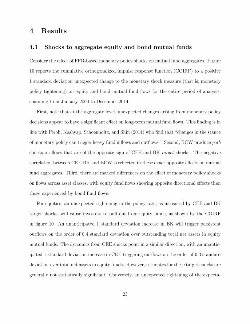
Consider the effect of FFR-based monetary policy shocks on mutual fund aggregates. Figure

10 reports the cumulative orthogonalized impulse response function (COIRF) to a positive

1 standard deviation unexpected change to the monetary shock measure (that is, monetary

policy tightening) on equity and bond mutual fund flows for the entire period of analysis,

spanning from January 2000 to December 2014.

First, note that at the aggregate level, unexpected changes arising from monetary policy

decisions appear to have a significant effect on long-term mutual fund flows. This finding is in

line with Feroli, Kashyap, Schoenholtz, and Shin (2014) who find that “changes in the stance

of monetary policy can trigger heavy fund inflows and outflows.” Second, BCW produce path

shocks on flows that are of the opposite sign of CEE and BK target shocks. The negative

correlation between CEE-BK and BCW is reflected in these exact opposite effects on mutual

fund aggregates. Third, there are marked differences on the effect of monetary policy shocks

on flows across asset classes, with equity fund flows showing opposite directional effects than

those experienced by bond fund flows.

For equities, an unexpected tightening in the policy rate, as measured by CEE and BK

target shocks, will cause investors to pull out from equity funds, as shown by the COIRF

in figure 10. An unanticipated 1 standard deviation increase in BK will trigger persistent

outflows on the order of 0.4 standard deviation over outstanding total net assets in equity

mutual funds. The dynamics from CEE shocks point in a similar direction, with an unantic-

ipated 1 standard deviation increase in CEE triggering outflows on the order of 0.3 standard

deviation over total net assets in equity funds. However, estimates for these target shocks are

generally not statistically significant. Conversely, an unexpected tightening of the expecta-

23

tions about future monetary policy as given by BCW’s path factor, which can be interpreted

as a better-than-expected economic outlook, will cause cumulative inflows into equity funds

of about 0.5 standard deviation, and they will persist over the subsequent months.17

For bond mutual funds, an unexpected tightening in the policy rate, as measured by the

target shocks, CEE and BK, will cause investors to add to bond funds, as shown by the

middle-left and middle panels in figure 10. As before, BCW shocks have the opposite effect

on flows than monetary policy measures capturing unexpected changes to the target rate. In

particular, an unanticipated 1 standard deviation increase in BCW will trigger cumulative

outflows on the order of 0.8 standard deviation over total assets. This effect on bond flows

is statistically significant and persistent.

In addition to the analysis on the effect of monetary policy on fund flows, we evaluate

the effect of a set of exogenous financial and macroeconomic variables that can be expected

to influence investors’ allocation decisions. First, we consider changes in our measure of

liquidity introduced by the Fed through unconventional monetary policy implementation.

Second, building on the literature that links demand for market liquidity and uncertainty,

we evaluate the effect of equity volatility shocks as proxied by the S&P 500 volatility index

(VIX) on mutual fund flows.18 Finally, we also compute the estimated effect of unexpected

changes in macro conditions, as captured by the first factor of the principal component

analysis (F1) introduced in section 2. The results are summarized in figure 11. The bottom

panels show the response functions of bond fund flows to unexpected changes in liquidity,

market volatility, and macroeconomic conditions. We find that shocks to Dlfed and Dlvix

produce large negative flows on bond mutual funds. Conversely, liquidity, volatility, and

17Hau and Lai (2016) show that declines in the local real short-term interest rates in eight countries fromthe Eurozone are associated with inflows into equity mutual funds and outflows into money market funds.

18Recent work by Huang (2015) argues that volatility can signal future equity fund flows and that periodsof higher expected market volatility can be associated with higher demand for liquidity, as managers aremore concerned with potential redemptions.

24

macroeconomic shocks are initially followed by equity fund outflows that fully revert over

the subsequent two months.

4.2 Mutual fund flows by investment strategy

The flow series used in the previous analysis aggregate flows from different investment cate-

gories at the asset-class level. For example, bond mutual funds include flows from different

strategies such as high-yield, investment-grade, and international bond funds. However, it

is important to recognize that strategies within the same asset class but with different risk

profiles and distinct investment goals might respond differently to unexpected changes in

the variables of interest. To this end, we next examine the effect of monetary, economic, and

financial shocks on flows at the investment-strategy level. As shown in figure 12, we find that

the negative relationship between bond flows at the aggregate level and shocks to the path

of monetary policy, as summarized by BCW, is also present at the investment-strategy level

for most taxable bond categories. In turn, a positive shock to the size of the Federal Re-

serve’s balance sheet is associated with persistent outflows from most bond fund categories,

with high yield being the only exception. As shown in figure 12, an unexpected increase

in liquidity will cause persistent large inflows into high-yield bond funds. In the context

of monetary policy easing, where the central bank is putting downward pressure on market

rates, these positive relationships could be associated with investors reaching for yield and

therefore shifting allocations to riskier assets. This result is similar to those observed across

equity strategies (figure 13). Interestingly, as depicted by column 3 in figure 12, shocks to

equity market volatility appear to have a large and persistent negative effect on high-yield

bonds. Conversely, the effect of equity market volatility on government bond fund flows is

slightly positive, although it lacks statistical significance.

For most of the fixed-income categories, positive shocks to macroeconomic conditions are

25

associated with initial inflows on the order of up to 0.5 standard deviation. However, these

initial positive effects revert over the following months, turning negative by the end of the

first half of the year. An exception to this pattern is high-yield funds, which experience an

initial outflow at the time of the shock but partially recover immediately after the shock.

Flows from equity strategies follow a similar pattern as high-yield flows (figure 13); however,

they manage to more than offset the initial outflows over the six months following the shock.

4.3 Flow-performance relationship

Over recent years, fixed-income investors have been pointing to a deterioration of market

liquidity conditions, particularly in the growing corporate bond market. Among the factors

explaining this new environment, asset managers frequently argue that new regulations on

liquidity and capital requirements have altered the willingness and capacity of dealers’ market

making. In this context, policymakers have been expressing concerns over potential risks to

financial stability that might arise in the event of a sudden run by mutual fund investors.

The underlying argument is that large redemptions in illiquid segments of the market can

add pressure to the performance of funds, as asset managers might be forced to sell less

liquid assets at a discount to meet redemptions. In the current regulatory setup, this decline

in the value of the fund portfolio will be borne by those who remain invested in the fund. As

a result, this “mutualization” of redemption costs could generate a first-mover advantage, as

investors have the economic incentive to redeem ahead of large outflows in order to avoid large

declines in the value of their fund shares. Policymakers are concerned about the amplifying

effects of large and sudden outflows on the underlying asset markets and the potential risks to

financial stability of such flows. In this context, a central question we explore in this section

is whether there is empirical evidence of a first-mover advantage in mutual fund investing

and how this evidence varies across fund strategies that are exposed to different levels of

26

liquidity mismatch. To address these questions, we build on the large and growing literature

on the flow-performance relationship and evaluate whether unexpected fund flows have an

effect on the value of the fund portfolio, as evidenced by performance.19 Recent studies

show mixed results about the existence of a first-mover advantage. For instance, using a

recursive VAR that orders first flows and then returns, Feroli, Kashyap, Schoenholtz, and

Shin (2014) find evidence of a first-mover advantage in some fund categories, such as those

investing in emerging market bonds, MBS, and investment-grade bonds for the 1998–2013

period. However, they find no evidence for U.S. Treasuries and domestic equities. Building

on Feroli, Kashyap, Schoenholtz, and Shin (2014), Plantier and Collins (2014) argue that

there is little evidence of a feedback effect from fund flows to fund returns (bond prices) when

the order of the endogenous variables in their VAR is altered. More recently, and focusing

on corporate bond funds, Goldstein, Jiang, and Ng (2015) show that fund flows are more

sensitive to poor performance than good performance and that this relationship is stronger

when market liquidity is limited. They argue that an illiquid corporate bond market may

give place to a first-mover advantage among mutual funds investing in this segment of the

market.20

Our baseline VAR model allows us to tackle this question in a unified manner, evaluating

the effect of monetary policy shocks on flows and the impact of these flows on performance,

therefore providing evidence on necessary conditions for the existence of a first-mover ad-

vantage. Again, we report results at the asset-class and investment-strategy levels.21 This

decision is guided by our interest in the aggregate price effect of mutual fund flows on fi-

19See Christoffersen, Musto, and Wermers (2014) for a review of the related literature.20Related work by Chen, Goldstein, and Jiang (2010) find that equity fund outflows are more sensitive to

underperformance in funds investing in illiquid assets than in funds investing in more liquid assets. Theyargue that strategic complementarities in mutual fund investing can be a source of financial fragility.

21Note that the baseline setup also includes contemporaneous and lagged equity and bond market returnsto control for changes in performance associated with developments in the underlying markets.

27

nancial markets and the potential threat of such flows to financial stability.22 Figures 14

and 15 show the response functions of fund performance to a positive 1 standard deviation

shock to the flow-to-assets ratio for bond and equity investment strategies. At the asset-

class level, results suggest that the price response to a positive shock to flows is substantially

different for bond and equity funds. Figure 14 shows that an unexpected inflow (outflow) of

1 standard deviation would have initially increased (decreased) bonds’ risk-adjusted return

by about 0.2 standard deviation and partially reverted this effect in the subsequent months,

but the price response of equity funds to a shock to flows of similar relative magnitude

is smaller and not statistically significant (figure 15). Results for equity funds are largely

driven by funds investing in domestic equities. However, a disaggregation by investment

strategy shows that the price effect of flows in emerging and international equity markets

is economically and statistically significant. In particular, a positive (negative) shock to

flows increases (decreases) performance by about 0.2 standard deviation in funds investing

in emerging equity markets. Response functions for international equity funds point in a

similar direction, although the effect on performance appears to be somewhat smaller than

in emerging markets funds. Overall, these results suggest that for less liquid segments of

the equity market, fund flows have an effect on performance that could potentially generate

a first-mover advantage and that under certain market conditions, large redemptions that

require asset managers to liquidate positions could amplify price pressures in underlying

asset markets.23

For bond mutual funds, results are generally economically and statistically significant

22Ideally, we would prefer higher-frequency data for the analysis of the price effect of fund flows. Nev-ertheless, monthly data allow us to explore this question. Also, investments decisions in bond and equitymutual funds are considered long-term investments, and in general, their associated entering and exitingcosts contribute to longer investment horizons. For example, as shown in table 1, a large fraction of mutualfund assets correspond to retirement assets, which are known to be stickier and can be expected to be lesssensitive to current market conditions.

23Note that results are symmetric by construction.

28

across investment strategies. As shown in figure 14, unexpected inflows on the order of

1 standard deviation over total assets have a positive effect on risk-adjusted returns on

the order of 0.15 standard deviation for investment-grade and government bond funds. In

particular, government bond funds have a slighter higher initial effect at around 0.2 standard

deviation that partially reverts over the subsequent months. Meanwhile, the price effect of

unexpected inflows into high-yield bond funds is also positive and statistically significant.

However, the risk-adjusted effect is slightly higher, at about 0.3 standard deviation, than

those experienced by the less risky government and investment-grade funds.24 International

and multisector bond funds present similar directional effects. However, their initial price

responses partially revert over the months following the shock. Interestingly, municipal bond

funds experience the strongest price effect, reaching 0.5 after the shock, retracing somewhat

after the fourth month, and stabilizing at around 0.3 standard deviation thereafter.25

Overall, although not conclusive, our findings provide empirical evidence of one of the

necessary conditions for the existence of run-like incentives for mutual fund investors, namely

the effect of fund flows on performance.

Another crucial aspect for a first-mover advantage to materialize is related to how port-

folio managers meet redemptions. In other words, investors’ incentives to redeem ahead of

large expected outflows also depend on the liquidity management practices of asset man-

agers, particularly, their tools and procedures to meet demand for liquidity that can arise

from both investors’ outflows and portfolio rebalancing. For instance, funds investing in

illiquid markets might build liquidity buffers at the fund or firm level to protect the value

24Performance is presented in risk-adjusted terms, accounting for the return volatility of the differentinvestment categories.

25Note that, as shown in table 6, the magnitudes of these price effects are consistenly smaller than theunderlying return volalitlity experienced by fund investors across investment strategies. For instance, whilethe initial response to outflows in the high yield universe is equivalent to a decline in performance in theorder of 64 basis points, the monthly return volatility of high yield mutual funds is about 355 basis pointsover the sample period spanning from January 2000 to December 2014.

29

of their portfolio from the need to liquidate assets at a discount in the case of large and

sudden redemptions by investors.26 Appropriate liquidity buffers can then help mitigate the

economic incentives that could trigger a first-mover advantage.

More recently, liquidity management practices also include a closer and more frequent

monitoring of the liquidity of the underlying assets in the portfolio (i.e. scoring), stress test-

ing and active communication strategies, among others. These new tools can help alleviate

the costs associated with traditional portfolio level liquidity buffers such as holding more

cash and liquid assets, which can be costly during normal times as they might hurt both

absolute and relative performance.

5 Conclusion

This paper investigates the effect of monetary policy shocks on mutual fund flows and the

risk to financial stability that might arise from these flows using a unified framework that

allows us to connect monetary policy, investors’ allocation decisions and performance. Em-

pirical results show that positive shocks to the path of monetary policy are associated with

persistent outflows from funds investing in the bond market. Specifically, a positive 1 stan-

dard deviation shock to the expectations about future monetary policy will translate to a

0.8 standard deviation increase in the flow-to-assets ratio. Conversely, the effect of monetary

path shocks on flow of funds investing in equity markets is positive, suggesting that a tighter-

than-expected monetary policy path, which could be interpreted as a better-than-expected

economic outlook, will cause net inflows into equity mutual funds. Within the bond fund

universe, results are mainly driven by the taxable bond segment of the market, including

government, high-yield, investment-grade, multisector, and world bond funds.

Our flow-performance results show that outflows can have an effect on the performance

26An alternative source of liquidity at the firm level might also include lines of credit from banks.

30

of funds investing in bonds and in less liquid segments of the equity market. In the current

regulatory environment, where redemption costs are mutualized and mutual funds engage

in liquidity transformation, our findings show that there are economic incentives that may

generate a first-mover advantage. However, adequate liquidity management practices and

policy guidelines can help mitigate these incentives.

Taken together, our findings show that monetary policy can have a direct effect on

mutual fund investors’ behavior, as evidenced by their fund flows, and that, under the

current regulatory set-up, there could be economic incentives for run-like behavior. As a

result, the potential risks to financial stability that mutual fund investors might generate

under stressed conditions should be weighed in the formulation of monetary policy.

31

References

Bernanke, B. S., and A. S. Blinder (1992): “The Federal Funds Rate and the Channels

of Monetary Transmission,” American Economic Review, 82(4), 901–21.

Bernanke, B. S., and K. N. Kuttner (2005): “What Explains the Stock Market’s

Reaction to Federal Reserve Policy?,” The Journal of Finance, 60(3), 1221–1257.

Buraschi, A., A. Carnelli, and P. Whelan (2014): “Monetary Policy and Treasury

Risk Premia,” .

Chen, Q., I. Goldstein, and W. Jiang (2010): “Payoff complementarities and financial

fragility: Evidence from mutual fund outflows,” Journal of Financial Economics, 97(2),

239–262.

Christiano, L. J., M. Eichenbaum, and C. Evans (1996): “The Effects of Monetary

Policy Shocks: Evidence from the Flow of Funds,” The Review of Economics and Statistics,

78(1), 16–34.

Christoffersen, S. E., D. K. Musto, and R. Wermers (2014): “Investor Flows to

Asset Managers: Causes and Consequences,” Annu. Rev. Financ. Econ., 6(1), 289–310.

Clarida, R., J. Gali, and M. Gertler (2000): “Monetary Policy Rules and Macroe-

conomic Stability: Evidence and Some Theory,” The Quarterly Journal of Economics,

115(1), pp. 147–180.

Coval, J., and E. Stafford (2007): “Asset fire sales (and purchases) in equity markets,”

Journal of Financial Economics, 86(2), 479–512.

DAmico, S., W. English, D. L. Salido, and E. Nelson (2012): “The Federal Re-

32

serve’s Large?scale Asset Purchase Programmes: Rationale and Effects,” Economic Jour-

nal, 122(564), F415–F446.

DAmico, S., and T. B. King (2013): “Flow and stock effects of large-scale treasury

purchases: Evidence on the importance of local supply,” Journal of Financial Economics,

108(2), 425 – 448.

Engen, E. M., T. Laubach, and D. L. Reifschneider (2015): “The Macroeconomic

Effects of the Federal Reserve’s Unconventional Monetary Policies,” (2015-5).

Feroli, M., A. K. Kashyap, K. L. Schoenholtz, and H. S. Shin (2014): “Market

Tantrums and Monetary Policy,” Research Paper 14-09, Chicago Booth.

Ferreira, M. A., A. Keswani, A. F. Miguel, and S. B. Ramos (2012): “The flow-

performance relationship around the world,” Journal of Banking & Finance, 36(6), 1759–

1780.

Gagnon, J., M. Raskin, J. Remache, and B. Sack (2011): “The Financial Market

Effects of the Federal Reserve’s Large-Scale Asset Purchases,” International Journal of

Central Banking, 7(1), 3–43.

Goldstein, I., H. Jiang, and D. T. Ng (2015): “Investor Flows and Fragility in Corpo-

rate Bond Funds,” Available at SSRN 2596948.

Gurkaynak, R. S., B. P. Sack, and E. T. Swanson (2005): “Do actions speak louder

than words? The response of asset prices to monetary policy actions and statements,”

International Journal of Central Banking.

Hamilton, J. D., and J. C. Wu (2012): “The Effectiveness of Alternative Monetary Policy

33

Tools in a Zero Lower Bound Environment,” Journal of Money, Credit and Banking, 44,

3–46.

Hau, H., and S. Lai (2016): “Asset Allocation and Monetary Policy: Evidence from the

Eurozone,” Journal of Financial Economics.

Huang, J. (2015): “Dynamic liquidity preferences of mutual funds,” in AFA 2009 San

Francisco Meetings Paper.

Huang, J., K. D. Wei, and H. Yan (2007): “Participation Costs and the Sensitivity of

Fund Flows to Past Performance,” The Journal of Finance, 62(3), 1273–1311.

Ippolito, R. A. (1992): “Consumer reaction to measures of poor quality: Evidence from

the mutual fund industry,” Journal of law and Economics, pp. 45–70.

Kuttner, K. N. (2001): “Monetary policy surprises and interest rates: Evidence from the

Fed funds futures market,” Journal of Monetary Economics, 47(3), 523–544.

Lou, D. (2012): “A flow-based explanation for return predictability,” Review of financial

studies, 25(12), 3457–3489.

Lucca, D. O., and E. Moench (2015): “The Pre-FOMC Announcement Drift,” The

Journal of Finance, 70(1), 329–371.

Musto, D. K., and A. W. Lynch (2003): “How Investors Interpret Past Fund Returns,”

The Journal of finance, 58(5), 2033–2058.

Plantier, L. C., and S. Collins (2014): “Are Bond Mutual Fund Flows Destabilizing?

Examining the Evidence from the Taper Tantrum,” Examining the Evidence from the

Taper Tantrum(September 1, 2014).

34

Rogers, J. H., C. Scotti, and J. H. Wright (2014): “Evaluating asset-market effects

of unconventional monetary policy: a multi-country review,” Economic Policy, 29(80),

749–799.

Rosa, C. (2012): “How "unconventional" are large-scale asset purchases? The

impact of monetary policy on asset prices,” Discussion paper.

Sims, C. A. (1992): “Interpreting the Macroeconomic Time Series Facts: The Effects of

Monetary Policy,” European Economic Review, 36(5), 975–1000.

Sirri, E. R., and P. Tufano (1998): “Costly search and mutual fund flows,” Journal of

finance, pp. 1589–1622.

Zheng, L. (1999): “Is money smart? A study of mutual fund investors’ fund selection

ability,” The Journal of Finance, 54(3), 901–933.

35

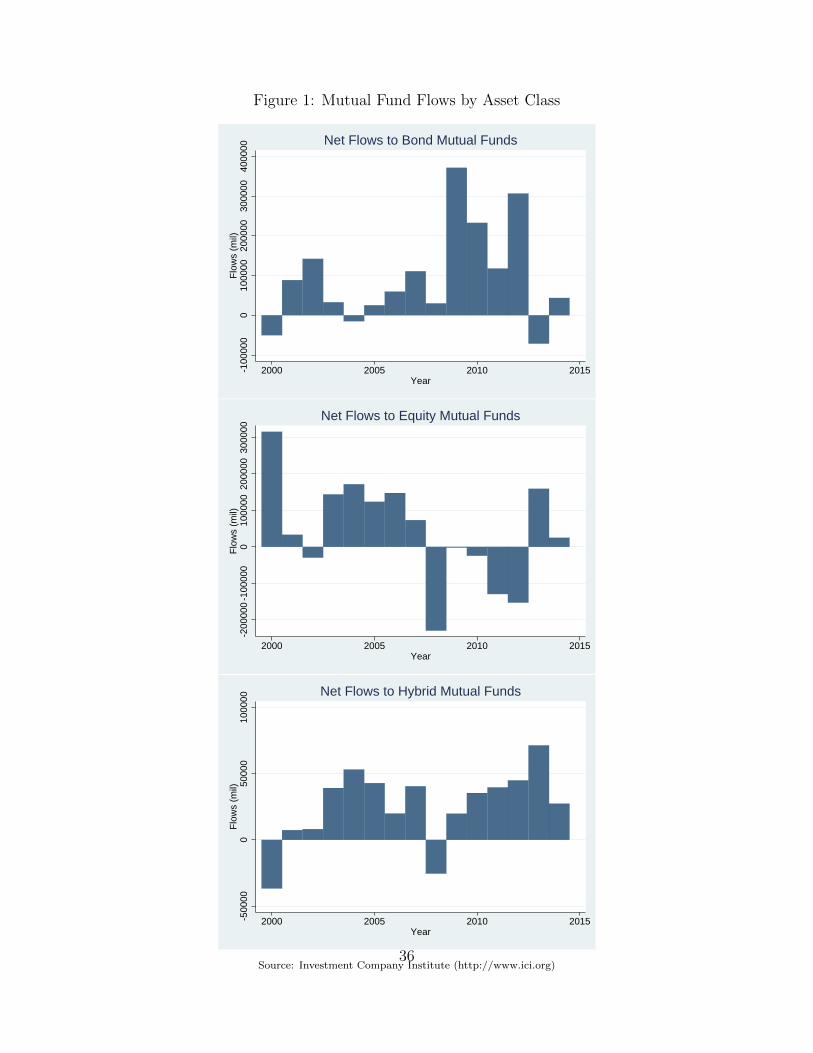
Figure 1: Mutual Fund Flows by Asset Class

-100

000

010

0000

2000

0030

0000

4000

00F

low

s (m

il)

2000 2005 2010 2015Year

Net Flows to Bond Mutual Funds

-200

000

-100

000

010

0000

2000

0030

0000

Flo

ws

(mil)

2000 2005 2010 2015Year

Net Flows to Equity Mutual Funds

-500

000

5000

010

0000

Flo

ws

(mil)

2000 2005 2010 2015Year

Net Flows to Hybrid Mutual Funds

Source: Investment Company Institute (http://www.ici.org)36

Figure 2: Bond Mutual Fund Flows by Investment Strategy

0-1

00,0

0010

0,00

020

0,00

0

2000 2001 2002 2003 2004 2005 2006 2007 2008 2009 2010 2011 2012 2013 2014

Investment Grade High YieldGovernment Bond Multi SectorWorld Bond Municipal Bond

Source: Investment Company Institute (http://www.ici.org)

37

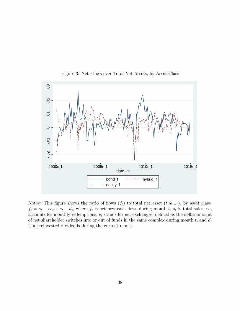
Figure 3: Net Flows over Total Net Assets, by Asset Class

-.02

-.01

0.0

1.0

2.0

3

2000m1 2005m1 2010m1 2015m1date_m

bond_f hybrid_fequity_f

Notes: This figure shows the ratio of flows (ft) to total net asset (tnat−1), by asset class.ft = st − ret + et − dt, where ft is net new cash flows during month t, st is total sales, retaccounts for monthly redemptions, et stands for net exchanges, defined as the dollar amountof net shareholder switches into or out of funds in the same complex during month t, and dtis all reinvested dividends during the current month.

38

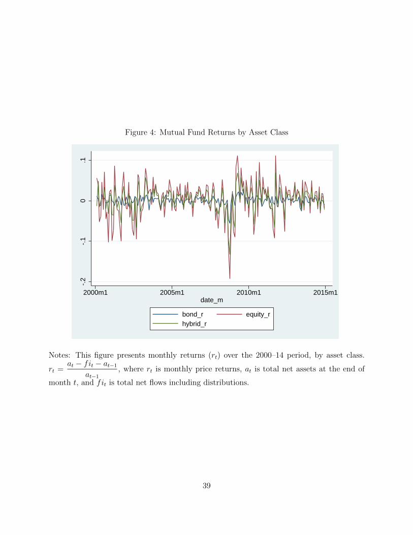
Figure 4: Mutual Fund Returns by Asset Class

-.2

-.1

0.1

2000m1 2005m1 2010m1 2015m1date_m

bond_r equity_rhybrid_r

Notes: This figure presents monthly returns (rt) over the 2000–14 period, by asset class.

rt =at − fit − at−1

at−1

, where rt is monthly price returns, at is total net assets at the end of

month t, and fit is total net flows including distributions.

39

Figure 5: Macro Factors, Principal Components

-4-2

02

4

2000m1 2005m1 2010m1 2015m1date_m

imputed f1 imputed f2imputed f3 imputed f4

Notes: This figure shows time series for a set of macroeconomic factors built using principalcomponents analysis. The below series are included in the analysis: Industrial Produc-tion (currip.B50001.s), Retail Sales (usslv i02yrf.m); Housing: Single-family Housing Starts,Single-family Housing Permits, Pending Home Sales, Existing Home Sales, CoreLogic PriceIndex for Single-Family Homes, 30-Year Conforming Fixed-Rate Mortgage; IS Manufactur-ing Survey: Average Regional New Orders, New Orders, Export Orders, Supplier Deliveries,Inventories; Consumer Surveys: Michigan Survey: Current Conditions, Michigan Survey:Expected Conditions, Consumer Sentiment- Michigan Index, Consumer Sentiment- Confer-ence Board Index, Expected Labor Market Conditions- Michigan Survey.

40

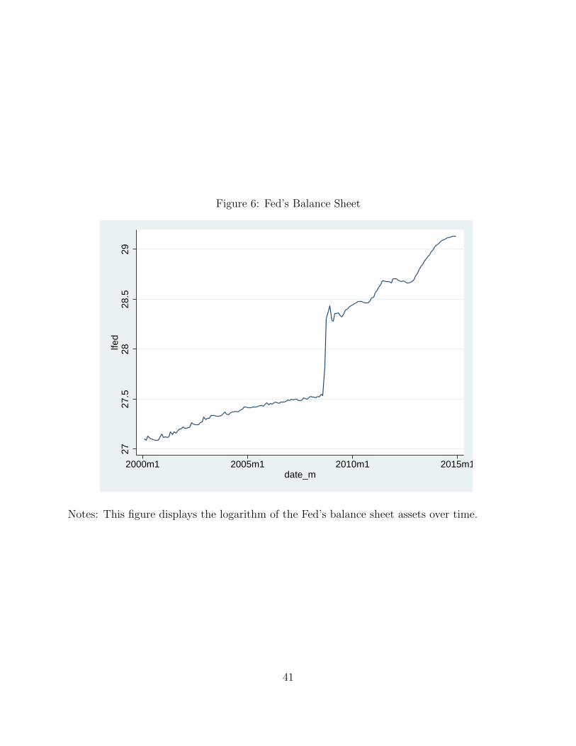
Figure 6: Fed’s Balance Sheet

2727

.528

28.5

29lfe

d

2000m1 2005m1 2010m1 2015m1date_m

Notes: This figure displays the logarithm of the Fed’s balance sheet assets over time.

41

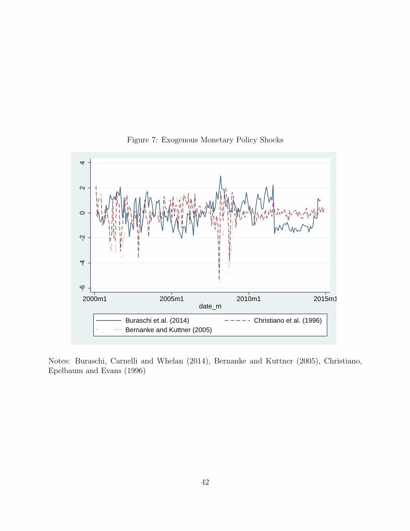
Figure 7: Exogenous Monetary Policy Shocks

-6-4

-20

24

2000m1 2005m1 2010m1 2015m1date_m

Buraschi et al. (2014) Christiano et al. (1996)Bernanke and Kuttner (2005)

Notes: Buraschi, Carnelli and Whelan (2014), Bernanke and Kuttner (2005), Christiano,Epelbaum and Evans (1996)

42

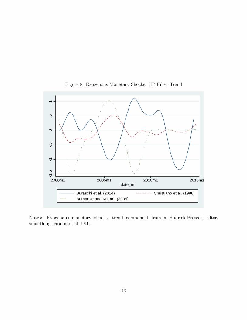
Figure 8: Exogenous Monetary Shocks: HP Filter Trend

-1.5

-1-.

50

.51

2000m1 2005m1 2010m1 2015m1date_m

Buraschi et al. (2014) Christiano et al. (1996)Bernanke and Kuttner (2005)

Notes: Exogenous monetary shocks, trend component from a Hodrick-Prescott filter,smoothing parameter of 1000.

43

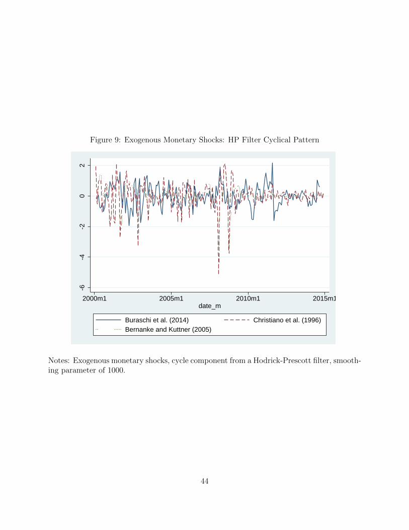
Figure 9: Exogenous Monetary Shocks: HP Filter Cyclical Pattern

-6-4

-20

2

2000m1 2005m1 2010m1 2015m1date_m

Buraschi et al. (2014) Christiano et al. (1996)Bernanke and Kuttner (2005)

Notes: Exogenous monetary shocks, cycle component from a Hodrick-Prescott filter, smooth-ing parameter of 1000.

44

Fig

ure

10:

Equit

yan

dB

ond

Mutu

alF

und

Flo

ws

-M

onet

ary

Pol

icy

Shock

s

Shock

:C

EE

Shock

:B

KShock

:B

CW

Equit

y

-.6

-.4

-.20

02

46

810

1214

1618

2022

24st

ep

90%

CI f

or c

oirf

coirf

irf: s

hock

_cee

->

e_f

-.8

-.6

-.4

-.20

02

46

810

1214

1618

2022

24st

ep

90%

CI f

or c

oirf

coirf

irf: s

hock

_bk

-> e

_f

0.51

02

46

810

1214

1618

2022

24st

ep

90%

CI f

or c

oirf

coirf

irf: s

hock

_bcw

->

e_f

Bon

d

0.51

02

46

810

1214

1618

2022

24st

ep

90%

CI f

or c

oirf

coirf

irf: s

hock

_cee

->

b_f

-.50.51

02

46

810

1214

1618

2022

24st

ep

90%

CI f

or c

oirf

coirf

irf: s

hock

_bk

-> b

_f

-1.5-1-.50

02

46

810

1214

1618

2022

24st

ep

90%

CI f

or c

oirf

coirf

irf: s

hock

_bcw

->

b_f

Th

isfi

gu

rere

port

sth

ecu

mu

lati

ve

ort

hogon

alize

dim

pu

lse

resp

on

sefu

nct

ion

s(I

RF

)of

equ

ity

an

db

on

dfu

nd

flow

sto

ap

osi

tive

1st

an

dard

dev

iati

on

shock

toth

eco

rres

pon

din

gm

on

etary

policy

mea

sure

.R

esp

on

ses

are

inm

onth

s.R

esu

lts

show

95%

con

fid

ence

inte

rvals

.

45

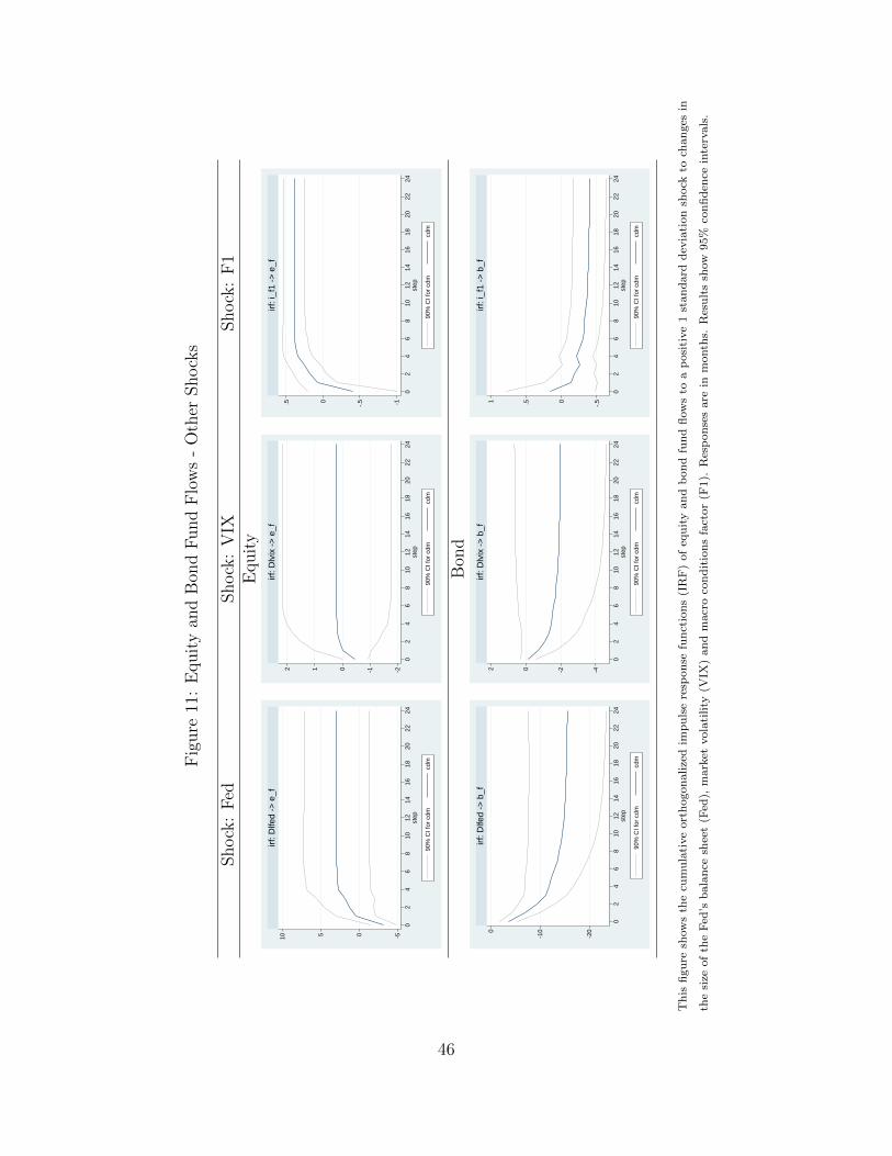
Fig

ure

11:

Equit

yan

dB

ond

Fund

Flo

ws

-O

ther

Shock

s

Shock

:F

edShock

:V

IXShock

:F

1E

quit

y

-50510

02

46

810

1214

1618

2022

24st

ep

90%

CI f

or c

dmcd

m

irf: D

lfed

-> e

_f

-2-1012

02

46

810

1214

1618

2022

24st

ep

90%

CI f

or c

dmcd

m

irf: D

lvix

->

e_f

-1-.50.5

02

46

810

1214

1618

2022

24st

ep

90%

CI f

or c

dmcd

m

irf: i

_f1

-> e

_f

Bon

d

-20

-100

02

46

810

1214

1618

2022

24st

ep

90%

CI f

or c

dmcd

m

irf: D

lfed

-> b

_f

-4-202

02

46

810

1214

1618

2022

24st

ep

90%

CI f

or c

dmcd

m

irf: D

lvix

->

b_f

-.50.51

02

46

810

1214

1618

2022

24st

ep

90%

CI f

or c

dmcd

m

irf: i

_f1

-> b

_f

Th

isfi

gu

resh

ow

sth

ecu

mu

lati

ve

ort

hogon

alize

dim

puls

ere

spon

sefu

nct

ion

s(I

RF

)of

equ

ity

an

db

on

dfu

nd

flow

sto

ap

osi

tive

1st

an

dard

dev

iati

on

shock

toch

an

ges

in

the

size

of

the

Fed

’sb

ala

nce

shee

t(F

ed),

mark

etvola

tili

ty(V

IX)

an

dm

acr

oco

nd

itio

ns

fact

or

(F1).

Res

pon

ses

are

inm

onth

s.R

esu

lts

show

95%

con

fid

ence

inte

rvals

.

46

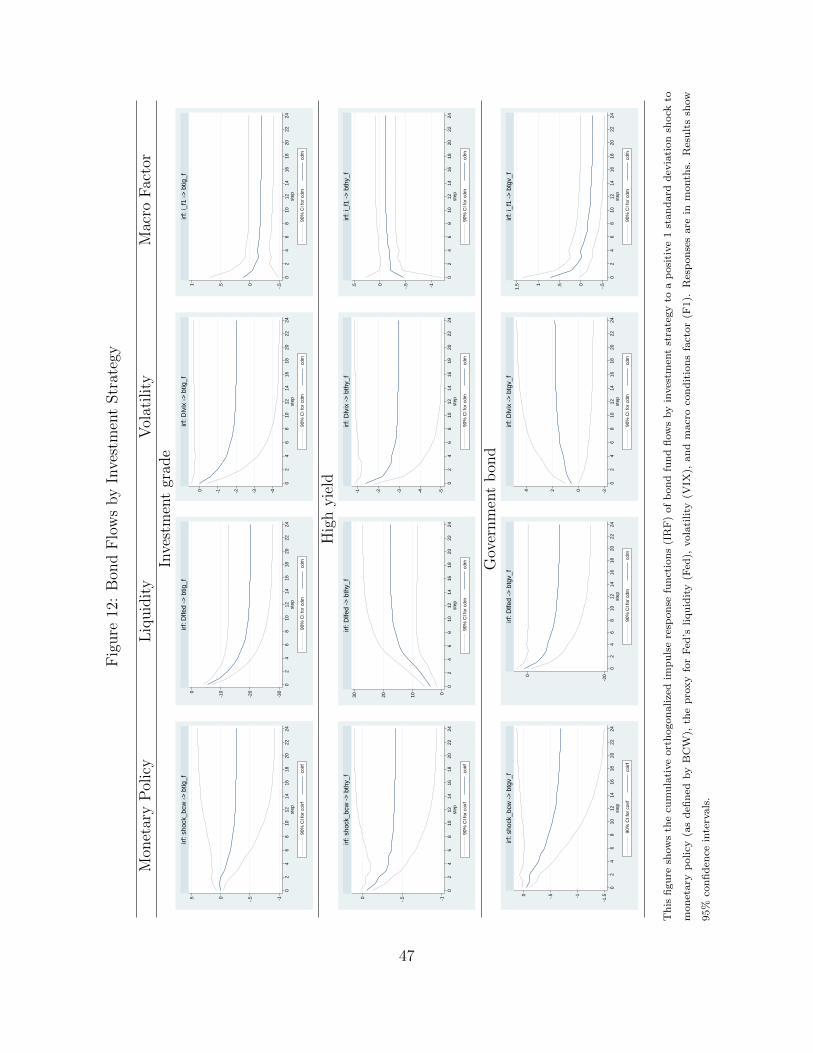
Fig

ure

12:

Bon

dF

low

sby

Inve

stm

ent

Str

ateg

y

Mon

etar

yP

olic

yL

iquid

ity

Vol

atilit

yM

acro

Fac

tor

Inve

stm

ent

grad

e

-1-.50.5

02

46

810

1214

1618

2022

24st

ep

90%

CI f

or c

oirf

coirf

irf: s

hock

_bcw

->

btig

_f

-30

-20

-100

02

46

810

1214

1618

2022

24st

ep

90%

CI f

or c

dmcd

m

irf: D

lfed

-> b

tig_f

-4-3-2-10

02

46

810

1214

1618

2022

24st

ep

90%

CI f

or c

dmcd

m

irf: D

lvix

->

btig

_f

-.50.51

02

46

810

1214

1618

2022

24st

ep

90%

CI f

or c

dmcd

m

irf: i

_f1

-> b

tig_f

Hig

hyie

ld

-1-.50

02

46

810

1214

1618

2022

24st

ep

90%

CI f

or c

oirf

coirf

irf: s

hock

_bcw

->

bth

y_f

0102030

02

46

810

1214

1618

2022

24st

ep

90%

CI f

or c

dmcd

m

irf: D

lfed

-> b

thy_

f

-5-4-3-2-1

02

46

810

1214

1618

2022

24st

ep

90%

CI f

or c

dmcd

m

irf: D

lvix

->

bth

y_f

-1-.50.5

02

46

810

1214

1618

2022

24st

ep

90%

CI f

or c

dmcd

m

irf: i

_f1

-> b

thy_

f

Gov

ernm

ent

bon

d

-1.5-1-.50

02

46

810

1214

1618

2022

24st

ep

90%

CI f

or c

oirf

coirf

irf: s

hock

_bcw

->

btg

v_f

-200

02

46

810

1214

1618

2022

24st

ep

90%

CI f

or c

dmcd

m

irf: D

lfed

-> b

tgv_

f

-2024

02

46

810

1214

1618

2022

24st

ep

90%

CI f

or c

dmcd

m

irf: D

lvix

->

btg

v_f

-.50.51

1.5

02

46

810

1214

1618

2022

24st

ep

90%

CI f

or c

dmcd

m

irf: i

_f1

-> b

tgv_

f

Th

isfi

gure

show

sth

ecu

mu

lati

ve

ort

hogon

alize

dim

pu

lse

resp

on

sefu

nct

ion

s(I

RF

)of

bon

dfu

nd

flow

sby

inves

tmen

tst

rate

gy

toa

posi

tive

1st

an

dard

dev

iati

on

shock

to

mon

etary

policy

(as

defi

ned

by

BC

W),

the

pro

xy

for

Fed

’sliqu

idit

y(F

ed),

vola

tility

(VIX

),an

dm

acr

oco

nd

itio

ns

fact

or

(F1).

Res

pon

ses

are

inm

onth

s.R

esu

lts

show

95%

con

fid

ence

inte

rvals

.

47

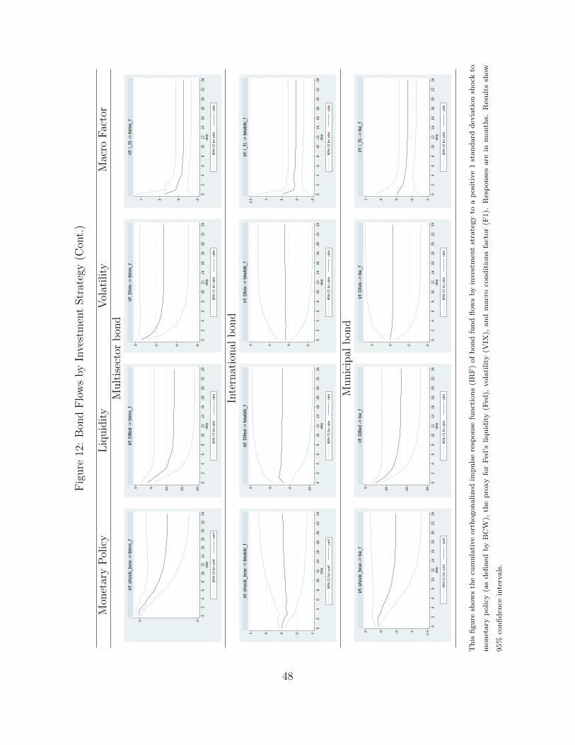
Fig

ure

12:

Bon

dF

low

sby

Inve

stm

ent

Str

ateg

y(C

ont.

)

Mon

etar

yP

olic

yL

iquid

ity

Vol

atilit

yM

acro

Fac

tor

Mult

isec

tor

bon

d

-20

02

46

810

1214

1618

2022

24st

ep

90%

CI f

or c

oirf

coirf

irf: s

hock

_bcw

->

btm

s_f

-20

-15

-10-50

02

46

810

1214

1618

2022

24st

ep

90%

CI f

or c

dmcd

m

irf: D

lfed

-> b

tms_

f

-6-4-20

02

46

810

1214

1618

2022

24st

ep

90%

CI f

or c

dmcd

m

irf: D

lvix

->

btm

s_f

-.50.51

02

46

810

1214

1618

2022

24st

ep

90%

CI f

or c

dmcd

m

irf: i

_f1

-> b

tms_

f

Inte

rnat

ional

bon

d

-1-.50.51

02

46

810

1214

1618

2022

24st

ep

90%

CI f

or c

oirf

coirf

irf: s

hock

_bcw

->

btw

bib_

f

-10-505

02

46

810

1214

1618

2022

24st

ep

90%

CI f

or c

dmcd

m

irf: D

lfed

-> b

twbi

b_f

-2024

02

46

810

1214

1618

2022

24st

ep

90%

CI f

or c

dmcd

m

irf: D

lvix

->

btw

bib_

f

-.50.51

1.5

02

46

810

1214

1618

2022

24st

ep

90%

CI f

or c

dmcd

m

irf: i

_f1

-> b

twbi

b_f

Munic

ipal

bon

d

-1.5-1-.50.5

02

46

810

1214

1618

2022

24st

ep

90%

CI f

or c

oirf

coirf

irf: s

hock

_bcw

->

be_

f

-30

-20

-100

02

46

810

1214

1618

2022

24st

ep

90%

CI f

or c

dmcd

m

irf: D

lfed

-> b

e_f

-4-202

02

46

810

1214

1618

2022

24st

ep

90%

CI f

or c

dmcd

m

irf: D

lvix

->

be_

f

-1-.50.51

02

46

810

1214

1618

2022

24st

ep

90%

CI f

or c

dmcd

m

irf: i

_f1

-> b

e_f

Th

isfi

gure

show

sth

ecu

mu

lati

ve

ort

hogon

alize

dim

pu

lse

resp

on

sefu

nct

ion

s(I

RF

)of

bon

dfu

nd

flow

sby

inves

tmen

tst

rate

gy

toa

posi

tive

1st

an

dard

dev

iati

on

shock

to

mon

etary

policy

(as

defi

ned

by

BC

W),

the

pro

xy

for

Fed

’sliqu

idit

y(F

ed),

vola

tility

(VIX

),an

dm

acr

oco

nd

itio

ns

fact

or

(F1).

Res

pon

ses

are

inm

onth

s.R

esu

lts

show

95%

con

fid

ence

inte

rvals

.

48

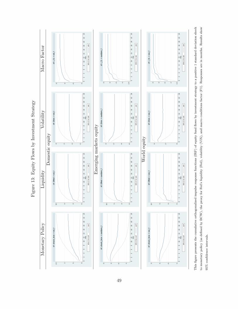
Fig

ure

13:

Equit

yF

low

sby

Inve

stm

ent

Str

ateg

y

Mon

etar

yP

olic

yL

iquid

ity

Vol

atilit

yM

acro

Fac

tor

Dom

esti

ceq

uit

y

0.51

1.5

02

46

810

1214

1618

2022

24st

ep

90%

CI f

or c

oirf

coirf

irf: s

hock

_bcw

->

ed_

f

-50510

02

46

810

1214

1618

2022

24st

ep

90%

CI f

or c

dmcd

m

irf: D

lfed

-> e

d_f

-2024

02

46

810

1214

1618

2022

24st

ep

90%

CI f

or c

dmcd

m

irf: D

lvix

->

ed_

f

-1-.50.5

02

46

810

1214

1618

2022

24st

ep

90%

CI f

or c

dmcd

m

irf: i

_f1

-> e

d_f

Em

ergi

ng

mar

kets

equit

y

-1-.50.5

02

46

810

1214

1618

2022

24st

ep

90%

CI f

or c

oirf

coirf

irf: s

hock

_bcw

->

ew

ldem

_f

-50510

02

46

810

1214

1618

2022

24st

ep

90%

CI f

or c

dmcd

m

irf: D

lfed

-> e

wld

em_f

-6-4-20

02

46

810

1214

1618

2022

24st

ep

90%

CI f

or c

dmcd

m

irf: D

lvix

->

ew

ldem

_f

-1.5-1-.50.5

02

46

810

1214

1618

2022

24st

ep

90%

CI f

or c

dmcd

m

irf: i

_f1

-> e

wld

em_f

Wor

ldeq

uit

y

-1-.50.5

02

46

810

1214

1618

2022

24st

ep

90%

CI f

or c

oirf

coirf

irf: s

hock

_bcw

->

ew

_f

-50510

02

46

810

1214

1618

2022

24st

ep

90%

CI f

or c

dmcd

m

irf: D

lfed

-> e

w_f

-4-20

02

46

810

1214

1618

2022

24st

ep

90%

CI f

or c

dmcd

m

irf: D

lvix

->

ew

_f

-1.5-1-.50.5

02

46

810

1214

1618

2022

24st

ep

90%

CI f

or c

dmcd

m

irf: i

_f1

-> e

w_f

Th

isfi

gu

rep

rese

nts

the

cum

ula

tive

ort

hogon

alize

dim

pu

lse

resp

on

sefu

nct

ion

s(I

RF

)of

equ

ity

fun

dfl

ow

sby

inves

tmen

tst

rate

gy

toa

posi

tive

1st

an

dard

dev

iati

on

shock

tom

on

etary

policy

(as

defi

ned

by

BC

W),

the

pro

xy

for

Fed

’sliqu

idit

y(F

ed),

vola

tility

(VIX

),an

dm

acr

oco

nd

itio

ns

fact

or

(F1).

Res

pon

ses

are

inm

onth

s.R

esu

lts

show

95%

con

fid

ence

inte

rvals

.

49

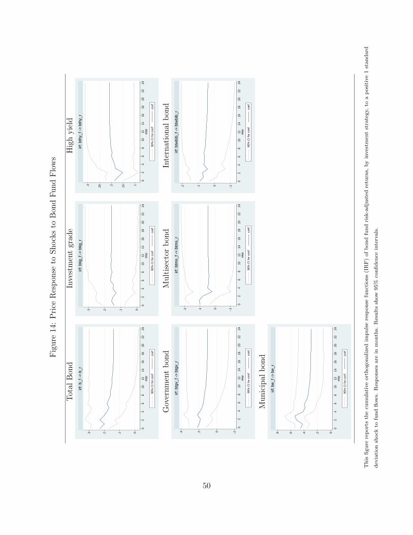
Fig

ure

14:

Pri

ceR

esp

onse

toShock

sto

Bon

dF

und

Flo

ws

Tot

alB

ond

Inve

stm

ent

grad

eH

igh

yie

ld

0.1.2.3

02

46

810

1214

1618

2022

24st

ep

90%

CI f

or c

oirf

coirf

irf: b

_f -

> b

_r

0.1.2.3

02

46

810

1214

1618

2022

24st

ep

90%

CI f

or c

oirf

coirf

irf: b

tig_f

->

btig

_r

.1.15.2.25.3

02

46

810

1214

1618

2022

24st

ep

90%

CI f

or c

oirf

coirf

irf: b

thy_

f ->

bth

y_r

Gov

ernm

ent

bon

dM

ult

isec

tor

bon

dIn

tern

atio

nal

bon

d

-.20.2.4

02

46

810

1214

1618

2022

24st

ep

90%

CI f

or c

oirf

coirf

irf: b

tgv_

f ->

btg

v_r

-.10.1.2

02

46

810

1214

1618

2022

24st

ep

90%

CI f

or c

oirf

coirf

irf: b

tms_

f ->

btm

s_r

-.10.1.2

02

46

810

1214

1618

2022

24st

ep

90%

CI f

or c

oirf

coirf

irf: b

twbi

b_f -

> b

twbi

b_r

Munic

ipal

bon

d

0.2.4.6.8

02

46

810

1214

1618

2022

24st

ep

90%

CI f

or c

oirf

coirf

irf: b

e_f -

> b

e_r

Th

isfi

gu

rere

port

sth

ecu

mu

lati

ve

ort

hogon

ali

zed

imp

uls

ere

spon

sefu

nct

ion

s(I

RF

)of

bon

dfu

nd

risk

-ad

just

edre

turn

s,by

inves

tmen

tst

rate

gy,

toa

posi

tive

1st

an

dard

dev

iati

on

shock

tofu

nd

flow

s.R

esp

on

ses

are

inm

onth

s.R

esu

lts

show

95%

con

fid

ence

inte

rvals

.

50

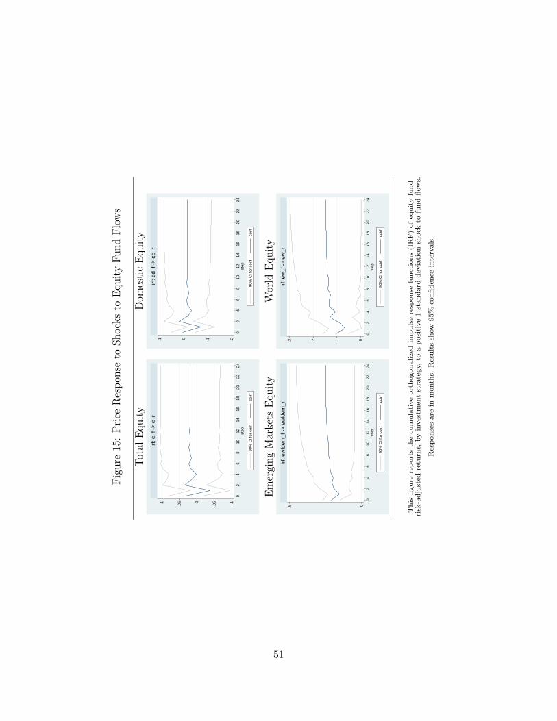
Fig

ure

15:

Pri

ceR

esp

onse

toShock

sto

Equit

yF

und

Flo

ws

Tot

alE

quit

yD

omes

tic

Equit

y

-.1

-.050

.05.1

02

46

810

1214

1618

2022

24st

ep

90%

CI f

or c

oirf

coirf

irf: e

_f -

> e

_r

-.2

-.10.1

02

46

810

1214

1618

2022

24st

ep

90%

CI f

or c

oirf

coirf

irf: e

d_f -

> e

d_r

Em

ergi

ng

Mar

kets

Equit

yW

orld

Equit

y

0.5

02

46

810

1214

1618

2022

24st

ep

90%

CI f

or c

oirf

coirf

irf: e

wld

em_f

->

ew

ldem

_r

0.1.2.3

02

46

810

1214

1618

2022

24st

ep

90%

CI f

or c

oirf

coirf

irf: e

w_f

->

ew

_r

Th

isfi

gu

rere

port

sth

ecu

mu

lati

ve

ort

hogon

alize

dim

pu

lse

resp

on

sefu

nct

ion

s(I

RF

)of

equ

ity

fun

dri

sk-a

dju

sted

retu

rns,

by

inves

tmen

tst

rate

gy,

toa

posi

tive

1st

an

dard

dev

iati

on

shock

tofu

nd

flow

s.

Res

pon

ses

are

inm

onth

s.R

esu

lts

show

95%

con

fid

ence

inte

rvals

.

51

Tab

le1:

Tot

alN

etA

sset

sby

Ass

etcl

asse

s(B

illion

sof

dol

lars

,ye

ar-e

nd)

2000

2001

2002

2003

2004

2005

2006

2007

2008

2009

2010

2011

2012

2013

2014

Panel

A:In

vestmen

tStrategy

Equ

ity

Fu

nd

sC

ap

ital

Ap

pre

ciati

on

1,4

34

1,1

05

766

1,0

41

1,1

49

1,2

33

1,3

19

1,4

20

809

1,0

86

1,2

48

1,1

78

1,3

19

1,7

25

1,8

56

Worl

d565

444

369

535

716

956

1,3

60

1,7

19

899

1,3

08

1,5

41

1,3

56

1,6

12

2,0

34

2,0

79

Tota

lR

etu

rn1,9

36

1,8

43

1,5

08

2,0

77

2,4

78

2,6

97

3,1

53

3,2

75

1,9

30

2,4

79

2,8

08

2,6

79

3,0

07

4,0

04

4,3

79

3,9

34

3,3

92

2,6

42

3,6

53

4,3

43

4,8

85

5,8

33

6,4

13

3,6

37

4,8

73

5,5

97

5,2

13

5,9

39

7,7

63

8,3

14

Bon

dF

un

ds

Inves

tmen

tG

rad

e246

311

406

474

518

570

640

760

736

1,0

50

1,2

41

1,3

65

1,5

72

1,4

51

1,5

25

Hig

hY

ield

110

109

108

159

168

159

176

176

118

198

243

271

342

420

378

Worl

d33

32

34

44

53

60

81

110

106

159

246

294

367

429

464

Gover

nm

ent

125

154

219

198

177

167

153

158

188

210

225

242

298

239

254

Mu

ltis

ecto

r32

37

43

50

56

62

80

101

85

131

160

174

231

248

273

Sta

teM

un

i132

140

153

149

144

147

154

156

135

159

156

159

178

145

156

Nati

on

al

Mu

ni

146

156

177

187

184

192

211

218

203

299

318

339

403

354

410

824

939

1,1

41

1,2

62

1,2

99

1,3

58

1,4

96

1,6

80

1,5

71

2,2

07

2,5

91

2,8

44

3,3

91

3,2

86

3,4

61

Hyb

rid

Fu

nd

s361

358

335

448

552

621

732

822

562

718

841

883

1,0

29

1,2

67

1,3

52

Tota

lL

on

g-t

erm

MF

s$5,1

19

$4,6

90

$4,1

18

$5,3

62

$6,1

94

$6,8

65

$8,0

60

$8,9

14

$5,7

71

$7,7

97

$9,0

29

$8,9

40

$10,3

59

$12,3

16

$13,1

27

Panel

B:In

vestorType

(ex.

MMF)

Ind

ivid

ual

Inves

tors

94%

94%

94%

94%

94%

93%

93%

93%

93%

92%

92%

92%

92%

92%

92%

Inst

itu

tion

al

Inves

tors

6%

6%

6%

6%

6%

7%

7%

7%

7%

8%

8%

8%

8%

8%

8%

Panel

C:Retirem

ent-relatedAssets

Sh

are

over

tota

lass

ets

37%

35%

34%

38%

40%

41%

42%

41%

36%

39%

42%

42%

43%

45%

46%

Panel

D:MutualFundConcentration

1995

2000

2005

2010

2011

2012

2013

Larg

est

5co

mp

lexes

34%

32%

37%

40%

40%

40%

40%

Larg

est

10

com

ple

xes

47%

44%

48%

53%

53%

53%

53%

Larg

est

25

com

ple

xes

70%

68%

70%

74%

73%

73%

72%

Note

s:T

his

tab

lesh

ow

sth

eev

olu

tion

of

tota

ln

etass

ets

of

lon

g-t

erm

mu

tual

fun

ds

from

2000

to2014,

by

ass

etcl

ass

.P

an

elA

rep

ort

sass

ets

by

inves

tmen

tst

rate

gy.

Pan

elB

pre

sents

the

share

of

ind

ivid

ual

an

din

stit

uti

on

al

ass

ets

over

tota

lass

ets

over

tim

e.P

an

elC

show

sth

esh

are

of

reti

rem

ent-

rela

ted

ass

ets

as

ash

are

of

tota

l

ass

ets.

Pan

elD

des

crib

esth

eco

nce

ntr

ati

on

of

the

larg

est

mu

tual

fun

dco

mp

lexes

.D

ata

isfr

om

the

Inves

tmen

tC

om

pany

Inst

itu

te.

52

Tab

le2:

Mutu

alF

und

Flo

ws

Sum

mar

ySta

tist

ics

Equ

ity

Hyb

rid

Bon

dIn

ves

tmen

tH

igh

Yie

ldM

ult

isec

tor

Worl

dB

on

dM

un

icip

al

Dom

esti

cW

orl

dE

ME

Equ

ity

Gra

de

Bon

dB

on

dE

qu

ity

Equ

ity

Panel

A:Fullsample

Mea

n3,4

97

2,1

58

7,7

77

3,9

82

526

1,2

20

1,3

12

665

-761

4,2

58

945

Max

56,7

10

12,5

26

47,1

85

24,2

84

11,7

49

6,6

11

17,3

34

10,3

23

34,0

04

23,9

29

6,1

84

Min

-70,4

99

-16,6

25

-60,0

10

-24,8

62

-15,5

92

-5,1

29

-7,7

02

-16,4

75

-48,7

90

-26,4

48

-4,3

00

p25

-6,4

62

472

-394

899

-1,0

82

147

-136

-806

-9,1

25

-28

-80

p50

5,6

60

2,6

23

7,5

93

3,4

83

675

608

792

1,0

78

-1,1

01

4,4

98

724

p75

14,7

36

4,2

33

15,5

59

7,3

34

2,6

30

2,4

75

2,5

83

2,7

34

7,9

42

8,5

56

1,9

42

Sta

nd

ard

Dev

.18,2

69

3,6

42

14,7

92

7,2

63

3,5

50

1,8

32

2,6

15

3,7

89

13,7

01

7,5

95

1,5

99

Skew

nes

s-0

.62

-0.9

4-0

.47

-0.6

0-0

.80

0.4

31.1

6-1

.36

-0.2

1-0

.44

0.1

3K

urt

osi

s4.6

36.8

35.4

05.7

66.8

23.9

110.6

06.9

93.7

84.7

14.2

5

Panel

B:Pre-crisis

Mea

n8,7

60

1,7

54

4,6

93

3,5

70

-126

325

617

438

3,8

16

4,9

44

593

Max

56,7

10

7,0

72

28,2

84

14,0

17

5,8

71

1,8

45

4,3

49

5,0

16

34,0

04

23,9

29

5,1

79

Min

-52,7

69

-7,3

05

-16,5

21

-2,0

27

-4,3

82

-1,2

61

-608

-5,1

09

-48,7

90

-17,7

13

-4,3

00

p25

446

399

-724

1,2

75

-1,5

60

-73

-136

-694

-3,5

86

307

-170

p50

9,5

59

2,1

35

4,7

32

3,2

18

-51

310

436

570

4,1

67

4,4

13

220

p75

18,9

86

3,6

66

9,1

93

5,5

55

1,1

15

625

1,0

60

1,6

78

12,1

11

9,1

30

1,0

93

Sta

nd

ard

Dev

.16,9

38

2,7

33

7,9

90

3,1

66

1,8

57

591

979

1,8

63

13,6

69

7,2

39

1,3

52

Skew

nes

s-0

.59

-0.8

70.0

70.6

50.2

30.2

61.5

2-0

.36

-0.5

60.2

50.4

9K

urt

osi

s4.9

94.1

73.2

63.3

93.3

73.1

95.8

93.2

14.7

23.4

55.5

1

Panel

C:Post-crisis

Mea

n-3

,705

2,7

11

11,9

98

4,5

46

1,4

18

2,4

43

2,2

62

974

-7,0

24

3,3

19

1,4

28

Max

37,5

98

12,5

26

47,1

85

24,2

84

11,7

49

6,6

11

17,3

34

10,3

23

18,5

56

19,0

42

6,1

84

Min

-70,4

99

-16,6

25

-60,0

10

-24,8

62

-15,5

92

-5,1

29

-7,7

02

-16,4

75

-44,0

51

-26,4

48

-3,9

35

p25

-15,6

83

727

2,8

34

71

-204

1,3

49

-156

-996

-13,8

37

-1,4

20

520

p50

-1,2

08

3,3

09

14,4

14

5,6

84

2,4

98

2,8

77

3,0

81

2,3

78

-6,4

56

4,8

36

1,5

63

p75

8,1

21

5,2

61

26,4

73

11,5

00

4,3

01

3,8

29

4,7

58

4,7

01

789

8,0

58

2,4

05

Sta

nd

ard

Dev

.17,6

52

4,5

68

20,0

82

10,5

63

4,8

94

2,2

14

3,6

63

5,4

15

11,0

75

8,0

11

1,7

85

Skew

nes

s-0

.81

-1.1

3-1

.00

-0.6

4-1

.22

-1.0

50.2

4-1

.25

-0.3

4-1

.09

-0.4

2K

urt

osi

s4.7

46.2

44.2

63.1

85.1

34.6

55.9

24.2

33.5

85.2

54.1

4

Note

s:T

his

tab

lesh

ow

ssu

mm

ary

stati

stic

sfo

rm

onth

lym

utu

al

fun

dfl

ow

s,by

ass

etcl

ass

(equ

ity,

hyb

rid

an

db

on

dfu

nd

s)an

dby

inves

tmen

tst

rate

gy.

Pan

elA

cover

s

the

full

sam

ple

per

iod

(2000–2014),

Pan

elB

the

pre

-cri

sis

per

iod

,an

dP

an

elC

the

post

-cri

sis

per

iod

.T

hes

ed

escr

ipti

ve

stati

stic

sare

calt

ula

ted

usi

ng

data

from

the

Inves

tmen

tC

om

pany

Inst

itu

te.

53

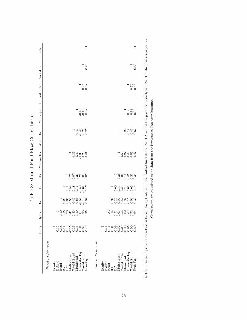
Tab

le3:

Mutu

alF

und

Flo

wC

orre

lati

ons

Equ

ity

Hyb

rid

Bon

dIG

HY

Mu

ltis

ecto

rW

orl

dB

on

dM

un

icip

al

Dom

esti

cE

q.

Worl

dE

q.

Em

eE

q.

Panel

A:Pre-crisis

Equ

ity

1H

yb

rid

0.1

21

Bon

d-0

.48

0.1

01

IG-0

.41

0.1

80.9

11

HY

0.1

90.2

30.3

30.1

11

Mu

ltis

ecto

r-0

.15

0.4

10.5

30.5

20.2

31

Worl

dB

ond

-0.2

50.3

20.4

20.4

8-0

.07

0.3

71

Mu

nic

ipal

-0.3

60.1

00.8

50.7

10.2

30.4

00.4

11

Dom

esti

cE

q.

0.9

10.0

1-0

.52

-0.5

00.2

3-0

.33

-0.4

3-0

.40

1W

orl

dE

q.

0.6

20.2

5-0

.14

-0.0

10.0

10.2

80.2

3-0

.10

0.2

41

Em

eE

q.

0.4

20.3

50.0

80.1

70.0

70.4

10.2

70.0

80.0

80.8

21

Panel

B:Post-crisis

Equ

ity

1H

yb

rid

0.7

11

Bon

d0.1

10.3

31

IG0.0

10.1

40.9

21

HY

0.3

90.5

10.2

30.0

01

Mu

ltis

ecto

r0.5

20.6

10.5

10.3

40.2

61

Worl

dB

ond

0.2

90.5

60.5

70.3

60.2

30.5

91

Mu

nic

ipal

-0.0

60.0

20.8

20.7

9-0

.15

0.2

70.2

41

Dom

esti

cE

q.

0.9

50.6

20.1

50.0

60.4

50.4

30.1

80.0

01

Worl

dE

q.

0.9

00.7

20.0

3-0

.06

0.2

30.5

50.4

0-0

.13

0.7

01

Em

eE

q.

0.6

00.6

40.3

00.1

50.3

40.4

70.6

20.0

40.4

60.6

91

Note

s:T

his

tab

lep

rese

nts

corr

elati

on

sfo

req

uit

y,hyb

rid

,an

db

on

dm

utu

al

fun

dfl

ow

s.P

an

elA

cover

sth

ep

re-c

risi

sp

erio

d,

an

dP

an

elB

the

post

-cri

sis

per

iod

.

Corr

elati

on

sare

calt

ula

ted

usi

ng

data

from

the

Inves

tmen

tC

om

pany

Inst

itu

te.

54

Tab

le4:

Mutu

alF

und

Ret

urn

s-

Sum

mar

ySta

tist

ics

Equ

ity

Hyb

rid

Bon

dIn

ves

tmen

tH

igh

Yie

ldG

over

nm

ent

Mu

ltis

ecto

rW

orl

dB

on

dM

un

icip

al

Dom

esti

cW

orl

dE

ME

Equ

ity

Gra

de

Bon

dB

on

dE

qu

ity

Equ

ity

Panel

A:Fullsample

Mea

n0.3

7%

0.2

6%

0.1

0%

0.1

8%

0.0

1%

0.0

5%

0.1

9%

0.2

5%

0.0

2%

0.4

0%

0.3

3%

0.7

4%

Max

11.1

8%

6.8

9%

3.4

7%

2.9

8%

18.5

2%

6.7

1%

4.2

2%

10.5

8%

4.2

2%

11.5

0%

12.9

2%

28.0

3%

Min

-19.2

1%

-13.2

4%

-5.5

4%

-4.8

0%

-17.8

2%

-4.2

5%

-8.7

4%

-10.5

2%

-5.4

4%

-18.3

5%

-21.7

9%

-28.1

2%

p25

-2.1

7%

-1.5

3%

-0.5

0%

-0.4

7%

-1.1

0%

-0.4

8%

-0.5

9%

-0.7

2%

-0.6

6%

-2.2

0%

-2.8

4%

-3.0

7%

p50

1.2

1%

0.5

6%

0.2

2%

0.2

6%

0.3

5%

0.1

0%

0.3

1%

0.2

7%

0.2

1%

1.1

1%

0.7

4%

1.0

1%

p75

3.5

3%

2.0

6%

0.7

4%

0.9

1%

1.0

6%

0.6

2%

0.9

4%

1.2

7%

0.7

7%

3.5

1%

3.5

7%

5.0

5%

Sta

nd

ard

Dev

.4.7

4%

2.9

9%

1.1

3%

1.0

8%

3.5

5%

1.0

1%

1.4

6%

2.3

0%

1.3

4%

4.6

8%

5.1

4%

7.0

6%

skew

nes

s-0

.68

-0.8

1-1

.10

-0.9

7-0

.22

0.8

7-1

.11

-0.0

1-0

.81

-0.6

8-0

.60

-0.3

9ku

rtosi

s4.0

75.1

37.3

56.0

413.9

713.1

79.8

79.2

46.1

73.9

34.3

35.4

6

Panel

B:Pre-crisis

Mea

n0.1

7%

0.2

0%

0.0

9%

0.2

0%

-0.1

8%

0.0

7%

0.2

3%

0.3

0%

0.0

4%

0.1

3%

0.3

5%

1.0

3%

Max

8.6

6%

5.7

8%

2.0

6%

2.3

3%

5.0

6%

1.4

6%

4.2

2%

5.4

4%

2.1

6%

8.8

9%

9.4

1%

11.4

2%

Min

-10.1

9%

-6.5

7%

-2.3

1%

-2.4

2%

-5.9

0%

-2.3

5%

-2.2

2%

-3.4

0%

-5.0

7%

-10.8

1%

-10.6

9%

-13.7

5%

p25

-2.2

8%

-1.4

7%

-0.4

5%

-0.4

8%

-1.1

8%

-0.4

1%

-0.4

8%

-0.6

3%

-0.6

6%

-2.2

6%

-3.1

2%

-3.0

7%

p50

0.5

8%

0.4

8%

0.2

0%

0.2

8%

0.2

5%

0.1

9%

0.2

8%

0.2

5%

0.2

7%

0.8

3%

0.9

7%

2.1

1%

p75

3.0

2%

1.6

9%

0.6

3%

0.8

7%

0.8

8%

0.5

7%

0.9

0%

1.1

9%

0.7

2%

2.7

9%

3.4

4%

5.0

5%

Sta

nd

ard

Dev

.4.1

7%

2.3

3%

0.8

3%

0.9

0%

1.8

8%

0.7

7%

1.1

2%

1.5

1%

1.1

0%

4.1

8%

4.2

9%

5.6

0%

Skew

nes

s-0

.50

-0.3

4-0

.34

-0.3

1-0

.31

-0.6

60.3

40.5

0-1

.19

-0.4

8-0

.44

-0.3

9K

urt

osi

s2.9

43.3

42.9

13.0

14.1

73.4

63.6

84.1

66.5

03.0

22.6

72.4

6

Panel

C:Post-crisis

Mea

n0.6

1%

0.3

4%

0.1

1%

0.1

5%

0.2

4%

0.0

3%

0.1

6%

0.1

9%

0.0

0%

0.7

2%

0.3

0%

0.4

1%

Max

11.1

8%

6.8

9%

3.4

7%

2.9

8%

18.5

2%

6.7

1%

3.8

4%

10.5

8%

4.2

2%

11.5

0%

12.9

2%

28.0

3%

Min

-19.2

1%

-13.2

4%

-5.5

4%

-4.8

0%

-17.8

2%

-4.2

5%

-8.7

4%

-10.5

2%

-5.4

4%

-18.3

5%

-21.7

9%

-28.1

2%

p25

-2.0

8%

-1.5

4%

-0.5

5%

-0.4

4%

-0.7

0%

-0.5

5%

-0.6

9%

-1.1

7%

-0.6

5%

-2.1

4%

-2.5

8%

-3.1

7%

p50

1.6

0%

0.7

9%

0.2

4%

0.2

0%

0.4

9%

-0.0

5%

0.3

2%

0.4

8%

0.1

9%

1.9

9%

0.4

8%

0.5

4%

p75

3.7

0%

2.5

8%

0.8

9%

0.9

5%

1.4

9%

0.6

6%

1.0

0%

1.4

7%

0.8

6%

3.9

2%

4.1

3%

4.6

1%

Sta

nd

ard

Dev

.5.3

6%

3.6

3%

1.4

1%

1.2

7%

4.8

3%

1.2

5%

1.7

8%

2.9

7%

1.5

8%

5.2

1%

6.0

1%

8.4

7%

Skew

nes

s-0

.81

-0.9

3-1

.18

-1.1

7-0

.29

1.2

4-1

.40

-0.0

4-0

.59

-0.8

5-0

.63

-0.3

0K

urt

osi

s4.3

34.6

16.3

26.0

68.8

912.1

48.9

76.9

15.1

84.2

64.2

75.1

8

Note

s:T

his

tab

lesh

ow

ssu

mm

ary

stati

stic

sfo

rm

onth

lym

utu

al

fun

dre

turn

s,by

ass

etcl

ass

an

dby

inves

tmen

tst

rate

gy.

Pan

elA

cover

sth

efu

llsa

mp

lep

erio

d

(2000–2014),

Pan

elB

the

pre

-cri

sis

per

iod

,an

dP

an

elC

the

post

-cri

sis

per

iod

.T

hes

ed

escr

ipti

ve

stati

stic

sare

calt

ula

ted

usi

ng

data

on

tota

ln

etass

ets

an

dn

etfl

ow

s

from

the

Inves

tmen

tC

om

pany

Inst

itu

te.

55

Tab

le5:

Mutu

alF

und

Ret

urn

Cor

rela

tion

s

Equ

ity

Hyb

rid

Bon

dIG

HY

Gover

nm

ent

Mu

ltis

ecto

rW

orl

dB

on

dM

un

icip

al

Dom

esti

cE

q.

Worl

dE

q.

Em

eE

q.

Panel

A:Pre-crisis

Equ

ity

1H

yb

rid

0.9

21

Bon

d0.1

40.2

31

IG-0

.02

0.0

70.9

31

HY

0.6

60.6

60.4

60.2

51

Gover

nm

ent

-0.2

7-0

.16

0.7

80.8

5-0

.06

1M

ult

isec

tor

0.3

10.3

80.7

70.7

00.4

50.5

21

Worl

dB

on

d0.3

50.3

70.7

10.6

50.4

60.4

30.7

11

Mu

nic

ipal

-0.0

80.0

30.8

30.7

10.1

50.6

80.5

30.4

11

Dom

esti

cE

q.

1.0

00.9

20.1

2-0

.03

0.6

5-0

.27

0.2

90.3

1-0

.08

1W

orl

dE

q.

0.9

40.8

60.1

90.0

40.6

5-0

.23

0.3

90.4

7-0

.06

0.9

11

Em

eE

q.

0.8

20.7

70.2

50.0

90.6

6-0

.17

0.4

80.5

1-0

.04

0.7

90.9

01

Panel

B:Post-crisis

Equ

ity

1H

yb

rid

0.9

81

Bon

d0.6

90.7

71

IG0.5

50.6

50.9

41

HY

0.7

10.7

70.8

20.6

61

Gover

nm

ent

-0.0

10.0

00.2

50.3

7-0

.24

1M

ult

isec

tor

0.6

10.6

20.6

00.4

90.4

20.3

21

Worl

dB

on

d0.7

60.8

30.8

80.7

60.9

0-0

.04

0.4

91

Mu

nic

ipal

0.0

40.0

40.3

30.3

6-0

.10

0.5

20.3

3-0

.09

1D

om

esti

cE

q.

1.0

00.9

70.6

60.5

30.7

1-0

.03

0.5

80.7

40.0

31

Worl

dE

q.

0.9

70.9

60.7

20.6

00.6

90.0

60.6

70.7

90.0

80.9

41

Em

eE

q.

0.8

80.9

00.8

10.6

90.8

6-0

.04

0.4

80.9

1-0

.03

0.8

50.9

01

Note

s:T

his

tab

lep

rese

nts

corr

elati

on

sfo

req

uit

y,hyb

rid

,an

db

on

dm

utu

al

fun

dre

turn

s.P

an

elA

cover

sth

ep

re-c

risi

sp

erio

d,

an

dP

an

elB

the

post

-cri

sis

per

iod

.

Corr

elati

on

sare

calt

ula

ted

usi

ng

data

from

the

Inves

tmen

tC

om

pany

Inst

itu

te.

56

Table 6: Price Responses and Underlying Asset Class Volatility

Initial Monthly Returns (%)Risk-adj. Effect Initial Effect Vol (stdv) Mean Min Max

Total Bond 0.23 0.261 1.134 0.10 -5.54 3.47Investment grade 0.15 0.163 1.084 0.18 -4.80 2.98High yield 0.18 0.639 3.552 0.01 -17.82 18.52Government bond 0.21 0.213 1.014 0.05 -4.25 6.71Multisector bond 0.10 0.146 1.461 0.19 -8.74 4.22International bond 0.90 2.751 3.057 0.40 -9.82 18.16Municipal bond 0.45 0.603 1.340 0.02 -5.44 4.22

Total Equity 0.04 0.166 4.744 0.37 -19.21 11.18Domestic Equity 0 0.000 4.683 0.40 -18.35 11.50Emerging Markets Equity 0.19 1.340 7.055 0.74 -28.12 28.03World Equity 0.10 0.514 5.139 0.33 -21.79 12.92

Notes: This table shows the initial price response (performance effect) of a positive 1 standard deviation shock to fund flows,

across investment strategies. Initial risk-adjusted effect is the initial effect on performance following the shock and is defined

in terms of return over standard deviation. Initial effect is the same as the risk-adjusted effect but expressed in percentage

terms. The final columns are summary statistics of the underlying monthly return series, by investment strategy, also in

percentage terms.

57