Embed Size (px)
Citation preview

Elise Botten
Marthe Kristine Hafsahl Karset
BI Norwegian School of Management-Thesis
GRA 19003 – MSc Thesis
Financial Constraints
for
Norwegian Non-Listed Firms
Date of submission:
01.09.2010
Campus:
BI Oslo
Programme:
Master of Science in Business and Economics
Major in Finance
Supervisor:
Bogdan Stacescu
This thesis is a part of the MSc programme at BI Norwegian School of Management. The school takes no
responsibility for the methods used, results found and conclusions drawn.

GRA 19003 Master Thesis 01.09.2010
Page i
Acknowledgements
The work on this thesis has been a valuable learning experience. Working with
this thesis has given us important knowledge and has been an interesting process.
We would like to thank our supervisor, Bogdan Stacescu, for important and
helpful guidance throughout the process of writing this thesis. Additionally, we
are thankful to the Centre of Corporate Governance Research for providing us
access to their comprehensive CCGR- database on non-listed and listed firms.
Oslo, 01.09.2010
_________________________ ___________________________
Elise Botten Marthe Kristine Hafsahl Karset

GRA 19003 Master Thesis 01.09.2010
Page ii
Abstract
In this paper we investigate non-listed companies in the context of financial
constraints. Our findings are varying, but we can find some tendencies.
We can observe that there are few indications that point towards some clear and
common characteristics of firms that are facing financial constraints. However, it
seems like smaller firms tend to be more financially constrained than larger firms,
and that non-listed firms might as well be facing the problem of financial
constraints. Dividend payout behavior seems to not be significantly related to the
probability of being financially constrained. On the other hand, our findings
indicate that firms considered as financially constrained tend to have more debt in
their capital structure.

GRA 19003 Master Thesis 01.09.2010
Page iii
Table of Content
Acknowledgements……………………………………………………..….i
Abstract…………………………………………………………………....ii
1. Introduction………………………………………………………………1
2. Literature Review………………………………………………………...3
2.1 Characteristics of non-listed firms…………………………………….3
2.2 Financial Constraints…………………………………………………..5
2.3 Previous research on financial constraints………………………….…6
2.4 Financial constraints and capital structure……………………….........9
2.5 Financial constraints and dividend theory………..…………………..12
2.6 Financial constraints and size………………………..……………….13
3. Methodology…………………………………………………...………….17
3.1 The Cash Flow Sensitivity of Cash…………………………………..17
3.1.1 The cash flow sensitivity of cash for listed vs.non-listed firms…19
3.1.2 The cash flow sensitivity of cash for firms who pay and do not pay
out dividends…………………………………………………………....19
3.1.3 The cash flow sensitivity of cash for the 20% smallest and the 20 %
largest firms……………………………………………………………20
3.1.4 The KZ-index for listed vs. non-listed firms………………...……20
3.1.5 Coparing the level of leverage for firms with high vs. low KZ-index
value…………………………………………………………………….22
3.1.6 The cash flow sensitivity of cash for high leverage vs. low leerage
firms…………………………………………………………………….22
3.2 Estimating Euler Equations for small vs.large firms………………...23
3.3 Testing for Heteroscedasticity………………………………………..26
4. Data………………………………………………………………………..28
4.1 Filtering………………………………………………………………29

GRA 19003 Master Thesis 01.09.2010
Page iv
5. Results…………………………………………………………………….32
5.1 The Cash Flow Sensitivity of Cash…………………………………..32
5.1.1 The cash flow sensitivity of cash for listed vs.non-listed firms…32
5.1.2 The cash flow sensitivity of cash for firms who pay and do not pay
out dividends…………………………………………………………....34
5.1.3 The cash flow sensitivity of cash for the 20% smallest and the 20 %
largest firms……………………………………………………………..36
5.1.4 The KZ-index for listed vs. non-listed firms……………………...38
5.1.5 Coparing the level of leverage for firms with high vs. low KZ-index
value…………………………………………………………………….39
5.1.6 The cash flow sensitivity of cash for high leverage vs. low leverage
firms…………………………………………………………………….40
5.2 Estimating Euler Equations for small vs.large firms………………...42
5.3 Testing for Heteroscedasticity………………………………………..42
6. Conclusion………………………………………………………………....44
7. Discussions………………………………………………………………...46
7.1 The new tax reform…………………………………………………..46
7.2 Using cash flow sensitivity of cash as a measure for financial
constraints……………………………………………………………..…47
7.3 Using a qualitative measure for financial constraints………………..48
7.4 Comments on the data used………………………………………..…49
Reference List……...…………………………………………………………....51
Attachments………..……………………………………………………………55
Preliminary Thesis Report………………………………………………………102

GRA 19003 Master Thesis 01.09.2010
Page 1
1. Introduction
The purpose of this Master Thesis is to study Norwegian non-listed firms. As we
have been introduced to during our master studies, non-listed firms represent a
huge part of the economy, as 80-90% of Norwegian firms are non-listed (Berzins,
Bøhren and Rydland. 2008). However, the research in this area is modest, as listed
firms still are the subject of the majority of financial studies. These facts provide
us with the incentive to study non-listed companies.
We have had a unique position in that we have had the possibility to access and
extract variables from the Centre of Corporate Governance Research- database.
This database consists of an interesting and comprehensive amount of data on
Norwegian non-listed firms.
We want to investigate non-listed companies in the context of financial
constraints. The importance of financial constraints has been discussed in several
papers, starting with Fazzari, Hubbard and Petersen (1988). Definitions of
financial constraints can be as follows: “A firm is considered more financially
constrained as the wedge between its internal and external cost of funds increases”
(Kaplan and Zingales. 1997, 172) and “frictions that prevent the firm from
funding all desired investments” (Lamount, Polk and Saá-Requejo. 2001, 529).
To our best knowledge, today there exist no studies on financial constraints on
non-listed companies in Norway. Furthermore, we do not find any research
concerning this subject on an international level either. We therefore find it
interesting to investigate non-listed companies in context with financial
constraints, as we think that this might be an important relationship to study.
We want to investigate if the relationship between non-listed and listed companies
in terms of financial constraints. We have chosen to focus on the hypothesis of
that non-listed firms probably have less access to external capital than listed firms,
and that they for this reason might be considered as more financially constrained
than listed firms are.

GRA 19003 Master Thesis 01.09.2010
Page 2
Furthermore, our intention is to explore non-listed firms and financial constraints
related to features like size, dividend- payout and leverage. According to previous
studies, we would expect that; small firms, firm who do not pay out dividends and
firms with high levels of leverage are most constrained.
We will test if these relationships give significant results, by applying the
framework of Almeida, Campello and Weisbach (2003), by using cash-flow
sensitivity of cash as a measure of financial constraints. Further, we applied the
framework of Tony M. Whited (1992), by using Euler equations.
This paper is organized as follows. Section 2 provides the Literature Review
where we give description of non-listed firms, definitions of financial constraints
and presents findings from previous studies within the field of financial
constraints and present financial theory that supports our further work and
hypothesis. In section 3, we present the methodologies we have applied.
Furthermore, in section 4 we describe the data we have used and how we have
worked with the dataset in order to compute the required variables, while we in
section 5, analyze the findings from our results. The outputs from our analysis are
to be found in the attachments. In section 6, we conclude our results. Finally, in
section 7 we have given a discussion concerning the results and tried to comment
more upon our findings and factors that may have influenced our results.

GRA 19003 Master Thesis 01.09.2010
Page 3
2. Literature Review
2.1 Characteristics of Non-listed Firms
Today, previous research on non-listed firms in terms of corporate finance and
governance in general is fairly modest compared to research on public firms.
Reasons for this might be that in most countries there is limited access to and
difficulties of collecting data on non-listed firms, and the fact that they do not
have a market price. However, in Norway, non-listed companies with limited
liability have to report full accounting statements (Berzins, Bøhren and Rydland
2008).
The importance of the economics of non- listed firms should not be overseen.
Non- listed companies amount to a huge part of the overall economy. About 80-90
% of all Norwegian firms are private firms, and they earn higher revenues, have
more employees and have two times the assets of public firms (Berzins et al.
2008).
In terms of companies in other European countries, a study done by Claessens and
Tzioumis (2006) in 19 European countries on ownership and financing structures
of listed and large non-listed corporations, revealed that non-listed companies
have higher returns on assets and equity compared to what listed companies have,
and that the non-listed firms had lower margins.
Furthermore, it is important to realize that non- listed firms differ from public
firms in many ways, and it is therefore need for separate research.
To understand the ways non-listed firms differs from listed firms, it is important
to identify the characteristics of non-listed firms compared to listed firms. The
main obvious distinctions between listed firms and non-listed firms, is that non-
listed have no market price, not for the firm nor for the equity of the firm. Non-
listed firms do not need to report quarterly earnings, and are therefore not
continuously priced as the listed companies are (Berzins et al. 2008).

GRA 19003 Master Thesis 01.09.2010
Page 4
Recent study on Norwegian listed and non- listed firms done by Berzins et
al.(2008) gives some valuable findings regarding characteristics of non-listed
firms compared to listed firms.
They find that non-listed firms have more and shorter maturity debt. Private firms
operate in a less open equity market, which can hamper the stock liquidity for the
owners. The less open equity market together with higher cost of capital of debt
for non listed firms, can lead to under-investment by the firms, and eventually it
might be harder for them to achieve equity finance.
Further, non-listed firms allocate a larger fraction of its earnings compared to
listed firms, which may be because the firms want to reduce the conflict of interest
between majority and minority owners.
In terms of economic performance, the paper states that non-listed firms have
higher accounting returns on assets (ROA) relative to listed firms. One possible
explanation for this might be that non-listed firms are more capital constrained, or
it may be due to less value- destroying short-termism in non-listed companies.
In terms of ownership structure, the ownership concentration tends to be greater in
non-listed firms.
Recent research by Berzins et al. (2008) also states that private and public firms
vary in terms of regulation. Minority owners in private firms can experience to be
less protected in private firms due to less regulation. Moreover, private firms are
less transparent than public firms, especially in terms of information.
Further, the study by Berzins et al. (2008) found that private firms, compared to
public firms, have more debt and shorter debt and higher dividends pr. unit of
earnings. Moreover, non-listed firms are small and often much smaller than the
public ones. However, the large firms tend to be private. 900 of Norway’s 1000
largest firms are in fact non-listed.
As one can see, there are distinct differences between the features of listed and
non-listed companies. Thus, transformation of research done on listed firms
cannot easily be transformed to count for non-listed firms as well. These
differences make it interesting to investigate non-listed firms.

GRA 19003 Master Thesis 01.09.2010
Page 5
2.2 Financial Constraints
There are several definitions of Financial Constraints. Kaplan and Zingales (1995)
give this definition: “A firm is financially constrained if the cost of availability of
external funds precludes the company from making an investment it would have
chosen to make had internal funds been available”. Furthermore, in 1997, Kaplan
and Zingales (1997; 172) gave this definition; “A firm is considered more
financially constrained as the wedge between its internal and external cost of
funds increases”.
Almeida et al. (2003) also gives a definition of financial constraints which is
interesting for the purpose of this thesis. Inspired by Keynes(1936;196), they
write that if a firm has unrestricted access to external capital, the firm is
financially unconstrained and there is no need to safeguard against future
investment needs and corporate liquidity becomes irrelevant.
According to Korajczyk and Levy (2003, 76) financially constrained firms are
defined as “firms that do not have sufficient cash to undertake investment
opportunities and that face severe agency costs when accessing financial
markets.”
Another definition given by Lamont, Polk and Saá-Requejo (2001, 529) describe
financial constraints to be “frictions that prevent the firm from funding all desired
investments.” These financial constraints may arise due to “credit constraints or
inability to borrow, inability to issue equity, dependence on bank loans or illiquid
assets.”
Summarizing these different definitions, one can say that financial constraints are
frictions like; agency costs (due to information asymmetries), difficulties of
getting loan, dependence of loans etc. that results in an arising wedge between
internal and external cost of funds. These frictions or costs of available funds can
prevent the firm from funding all the desired investment opportunities that it
would have invested in, had they had the funds needed. This turning-down of

GRA 19003 Master Thesis 01.09.2010
Page 6
positive NPV projects hampers the potential for important future economic
development and growth.
2.3 Previous research on financial constraints.
Over the past decades the role of financial constraints and how to capture the level
and significance of it have diverged considerably from one study to the next
during the years.
In terms of wanting to explore the relationship between effects of financial
constraints on firm behavior, early research has been concentrated around
corporate investment demand.
One of the first to do a study within the area of financial constraints was Fazzari,
Hubbard and Petersen (1988). In order to group companies as financial
constrained and not financial constrained, they categorized US companies
according to their payout behavior.
The paper suggests that when a firm experience financing constraints, investment
expenditures will tend to vary with the accessibility of internal finance, not only
with the availability of positive net present value projects. This method is widely
used in order to recognize the firms that are more affected by financing constraints
and opposite. Their results show that financial factors affect investments, and that
the link between financing constraints and investment varies by the type of firm.
Therefore, they suggest that one could study the impact of financing frictions on
corporate investment by comparing investment to cash flow sensitivities across
groups of companies categorized by a proxy for financial constraint. Their results
suggest that investment decisions of firms grouped as being more financially
constrained are more sensitive to the availability of internal cash flows, relative to
those grouped as being less constrained.
Number of subsequent studies has provided empirical evidence of the same.
However, this methodology of financially constrained firms being more
investment-cash-flow sensitive than those being less constrained has been
questioned. Kaplan and Zingales (1995) is one paper that questions the results of
Fazzari et al. (1988) and other previous studies using this methodology.

GRA 19003 Master Thesis 01.09.2010
Page 7
This paper also studies the relationship between the financing constraints and
investment- cash flow sensitivities, by investigating the Fazzari et al. (1988)
sample of low-dividend manufacturing firms with positive real sales growth.
Their main striking finding is that firms they categorize as being less financially
constrained, exhibit significantly greater sensitivities than firms categorized as
more financially constrained. They state that their findings point toward that
higher sensitivity cannot necessarily be understood as proof that they are more
financially constrained. They argue that this should not be so shocking, as they
claim that there should be no strong theoretical reason for investment-cash flow
sensitivities to increase monotonically with the degree of financing constraints.
However, the paper by Kaplan and Zingales (1995) has again been subject to
criticism. Schiantarellii (1995) states that Kaplan and Zingales’ classifications of
unconstrained and constrained companies are of subjective nature. Schiantarelli
also criticizes Fazzari et al’s classifications, which uses prevalent dividend payout
behavior as their basis.
Other studies finding contradicting result to and calls into question the findings of
Fazzari et al. (1988) are Kadapakkam et al. (1998) and Cleary (1999 and 2006).
Kadapakkam et al., investigates companies in Canada, France, Germany, Great
Britain , Japan and the USA and find that large firms are more cash flow –
investment sensitive than smaller firms, and conclude that cash flow- investment
sensitivity is not an accurate measure of its access to capital markets (same as
Kaplan et al 1997 did), Cleary’s findings also support the conclusions of Kaplan
and Zingales (1997); companies with stronger financial positions tend to be more
investment- cash flow sensitive than those companies with weaker financial
positions. Further, findings point to that companies with higher payout- ratios are
more investment- cash flow sensitive than those with lower ratios.
In the paper “Financial constraints and investment”, Fabio Schiantarelli (1995)
investigates the methodological issues involved in testing for financial constraints
on the basis of Q models of investments. He finds that the essential problem in
using Q models in this matter is that average Q may be a very inaccurate
alternative for the shadow value of an additional unit of new capital. He suggests
addressing this problem by estimating the Euler equation for the capital stock

GRA 19003 Master Thesis 01.09.2010
Page 8
derived from the underlying model. The benefit of the Euler equation approach is
that it avoids relying on measures of profitability based on a firm’s market value.
Almeida et al. (2003) tests a sample of 3547 publicly- traded manufacturing
companies in the period 1971- 2000. They used the link between financial
constraints and a company’s demand for liquidity in order to develop an analysis
of the impact of financial constraints on firm policies. Their starting point is that
firms who are financially constrained need to save more of their incoming cash
flows in order to be able to take on positive NPV projects as they appear. The
effect of financial constraints can therefore be captured by a firm’s propensity to
save cash out of incremental cash flows. They have called this effect “the cash
flow sensitivity of cash”. Their main finding confirms this hypothesis; firms that
are more likely to be financially constrained, exhibit a significantly positive cash
flow sensitivity of cash, while the unconstrained companies do not.
Whited (1992) contributes with another important paper in the context of financial
constraints (liquidity constraints). She investigates the investment behavior of
firms when they maximize their value subject to borrowing constraints. The
hypothesis is that due to the asymmetric information theory in debt markets, weak
small firms with low liquid assets positions have limited access to debt markets.
By using an Euler equation as an optimizing model of investment, the paper
concentrates on the question of interdependence of finance and investment. By
concentrating on debt finance, the paper expands the work of Fazzari et al (1988).
Findings point towards that difficulties in achieving debt finance, do have an
impact on investment behavior. Furthermore, the effect of financial constraints
tends to be more binding for firms that do not participate in the bond market.
Whited further developed her work, together with GuojunWu in 2003. In their
article, “Financial Constraints Risk”, Whited and Wu (2003) also use investment
Euler equations. Some of their findings are that the constrained companies tend to
earn higher returns.

GRA 19003 Master Thesis 01.09.2010
Page 9
2.4 Financial Constraints and Capital Structure
Based on earlier mentioned definitions of financial constraints, one might say that
financial constraints are highly related to the differences between the cost of
internal- and external finance, and consequently also the composition of capital
structure.
Thereby, in order to understand the relevance of financial constraint, one has to
understand theories concerning capital structure. Capital structure is about how a
firm finances its actions and prospective growth by the use of different finance
sources, and it is the composition of a company's debt and equity. In addition it
can contribute to maintain liquidity in case of investment opportunities (Mjøs
2008). Furthermore, capital structure choices differ across firms and over time.
The modern theory of capital structure has its origin in the Modigliani- Miller
paper. According to the Modigliani Miller Irrelevance substitutes Theorem
(1958), in perfect capital markets, a company’s capital structure should be
unrelated to its value; it is irrelevant. Internal and external finances is therefore
claimed to be perfect substitutes, and the company’s financing and investment
decisions should not be affected by the firms’ capital structure. In other words; in
perfect capital markets, the company’s financial composition should not have an
effect on its value.
However evidence from studies done after Modigliani and Miller point towards
the existence of imperfections like; informational asymmetries, agency problems,
contract enforcement problems, transaction costs, tax advantages and costs of
financial distress. Thus, the irrelevance hypothesis fails to perform; there are
capital markets imperfections (Schiantarelli 1995). Access to new debt or equity
finance, the accessibility to internal finance, dividend payment and the
functioning of credit markets are factors that may affect investment behavior, thus
also the capital structure of companies (Fazzari et al. 1988).
These imperfections results in that the costs of external and internal finance are
not perfect substitutes. With the presence of this situation, one might say that
financial constraints exists (Schiantarelli 1995).

GRA 19003 Master Thesis 01.09.2010
Page 10
In our context, based on the purpose of our analysis, we choose to elaborate on the
imperfections of asymmetric information and agency problems.
The asymmetric information approach contributes in explaining the composition
of a company’s capital structure and therefore also, the “imperfection” between
external and internal finance. This approach relates to a situation where one party,
say firm managers or insiders, are supposed to have private and better information
about the characteristics of the firm’s return stream or/ and investment
opportunities, than the other party (Stiglitz and Weiss 1981;Myers 1984;Stulz
1990). This asymmetry leads to a costly and almost impossible assignment for
suppliers of external finance to estimate the true worth of companies’ investment
opportunities; therefore it can produce significant cost disadvantages of external
finance for some types of companies. This asymmetric information can give rise
to numerous problems. A special case of asymmetric information- problem is
moral hazard. Moral hazard refers to a situation where agent may not act in the
principals best interests. Extravagant investments, insufficient effort, self-dealing
and entrenchment strategies are all actions labeled as moral hazard (Tirole 2006).
These are activities where the manager may exploit the asymmetric information
balance in a negative way for the firm, thereby creating costs disadvantages of
external finance for the company (Stulz 1990)
In the context of information asymmetries and determinants of capital structure,
principal- agent problems are relevant. Principal-agent problems refer to a
situation where agency costs can arise. Agency costs can arise due to conflict of
interest between different stakeholders of the company. This point of view is often
referred to as the agency approach. Earlier research of Jensen and Meckling
(1976) which build on previous studies by Fama and Miller, categorize the
conflict into conflicts between equity holders and managers and conflicts between
debt holders and equity holders.
The conflict between equity holders and managers can arise if managers hold less
than 100% of the residual claim. In this situation, the managers can capture the
entire gain from profit enhancement activities, but do not take the entire cost of
these activities. This might lead to personal benefits for the manager.
This inefficiency can be reduced if a larger part of the firm’s equity is owned by
the manager. (Harris and Raviv 1991)

GRA 19003 Master Thesis 01.09.2010
Page 11
The other type of conflict; between debt holders and equity holders can arise when
the agent have superior information about its projects and possible investments
and possible actions to take, relative to potential investors. If this superior
information leads to the equity holder having incentives to invest suboptimal and
derive incomplete debt contracts, agency cost of debt finance rises (Harris and
Raviv 1991).
Moral hazard can be an explanation to the agency cost of debt. High levels of debt
can tempt the managers and equity holders to choose excessively risky projects
(Jensen and Meckling 1976; Whited 1992). The presence of limited liability of
debt is features that can help explain why moral hazard problem and agency cost
of debt arise. The limited liability feature of debt contracts refers to a situation
where the borrower has limited liability relative to the lenders of funds. If the
funded project/investment fails, debt holders will bear most of the costs/
consequences. It can also lead the managers and equity holders to accept project
with higher risk, thus higher possible returns. Therefore, this limited liability can
create incentives for managers to behave counter the interests of creditors (Fazzari
et al. 1988).
This problem will increase the cost of debt and might lead to credit rationing in
the debt market. Credit rationing can occur due to “adverse selection” (Myers and
Majluf 1984). If there is an asymmetric problem where managers have private
information relative to the providers of the fund, lenders cannot distinguish
between good and bad borrowers. It can lead to a situation where interest rate rise
and loan size may be limited; thus, the company has to obtain the external finance
at a premium. (Stigliz and Weiss 1981;Whited 1992)
However, having debt can also contain positive aspects. Having a proportion of
debt forces the management to pay out a steady cash flow to its creditors. This
obligation lowers investment in all natures of the world, and reduces investments
when it else might have been too high and risky (Stultz 1990).
The Pecking-Order-Theory, as first described by Myers and Majuf (1984) can also
help explain why different finance sources not are perfect substitutes. This theory
categorizes the several forms of finance into a hierarchy. The theory states that

GRA 19003 Master Thesis 01.09.2010
Page 12
due to the information asymmetry, companies will choose this order of financing;
First use retained earnings and fund of current owners, then risk- free and risky
debt and last raising new equity (Mjøs 2008).
Capital structure is therefore a result of many different factors, and these factors
again depend on what type of company one talk about; whether it is a listed, non-
listed, small, large, dividend paying company or not etc. The factors mentioned
(asymmetric info, agency cost) will affect and influence different types of
companies in different ways, therefore leading to various capital structures. These
differences are highly relevant for the explanation of why financial constraint may
appear and not. The theories above help enlighten the reasons why different types
of companies have different cap structures.
2.5 Financial Constraints and Dividend Theory
Paying dividend can serve many purposes, both negative and positive. Paying
dividend can be done in order to signal the company’s prospects or true worth. A
dividend payout larger than expected may for example indicate beliefs of the firm
doing better and of higher earrings in the future. This action can also signal that
the firm does not have any positive NPV projects to invest in.
Furthermore, paying dividends can indicate good news because it decreases the
amount of free cash flow in the firm, thus reducing potential agency costs. This
view is often referred to as the agency model of dividends.
A decrease in dividends may signal the opposite, namely indicate that firm is
doing worse and potential for lower earnings. Moreover, as a firm matures, it
might experience the investment opportunities shrinking, which again can lead to
a natural increase in dividends. Then investors possibly will consider this increase
as good news, while it in reality might be a sign of decreasing profitability.
Furthermore, the market tends to react positively to message of dividend increase,
while negatively to a decrease in dividends.
In periods when a company faces large growth opportunities, companies should
cut back or avoid paying dividends (Allen and Michaely 2002).

GRA 19003 Master Thesis 01.09.2010
Page 13
There exists three groups that are likely to be affected most by a firm’s dividend
policy; shareholders, management and bondholders. Paying dividends can lead to
interest conflicts between the groups and lead to agency costs for the firm.
Allen and Michaely (2002) found that payout policies are in fact not driven by the
desire to signal the value of the firm, rather they found evidence of that payout
policy was influenced of wanting to avoid potential overinvestment by managers.
Mjøs (2008) characterize dividend- payment to be “a strong indicator of financial
health”. Furthermore, he describes that dividend- payers tend to not be financially
constrained and that these groups use a less amount of debt. He also states that
these firms have total returns that are twice of those firms not paying dividend.
Almeida et al. (2003; 14) groups constrained firms as firms who have
significantly lower payout rations than unconstrained firms. This is the same
intuition as proposed by Fazzari et al. (1988).
However, Berzins and Bøhren (2008) found that private (non-listed) firms tend to
have higher dividends per unit of earnings compared to public firms in the year
2005.
Summarizing the earlier findings presented her, one can see that the majority of
the research point towards that firms who are paying dividend tend to show sign
of being financially unconstrained. Moreover constrained firms seem to pay lower
ratios of dividends than unconstrained companies do.
2.6 Financial Constraints and Size
Size is an important and thoroughly discussed variable in connection to financial
constraints.
There are done several analysis on the connection between financial constraints
and the variable size. Furthermore, size has often been used as an a priori measure
in order to categorize companies into more or less constrained groups.

GRA 19003 Master Thesis 01.09.2010
Page 14
Hu and Schiantarelli’s (1994) study on quoted companies between 1978 and 1987,
find that size is positively correlated to the likelihood of being financially
constrained.
Results from studies done by Cleary (1999; 2006) point towards firms being
categorized as not financially constrained according to financial strength, are
likely to be larger and also have higher pay-out ratios, but the connection is not
outstandingly strong.
Schiantarelli (1995) finds that size tends to be a useful criterion in order to
recognize firms that are more probable to be financially constrained. Further he
states that this is only when the sample used for estimation includes at least a part
of the lower tail of the size distribution.
Korajczyk and Levy (2003) states that previous literature often use size and
degree of bank dependence as proxies for the level of financial constraints, and
that it is consistent with that facing greater financial constraints makes it difficult
to borrow in order to smooth cash flows following negative shocks to the
economy.
Whited and Wu (2003) find evidence of that firms that are classified as not
financial constrained, typically are large and liquid.
However, Fazzari et al. (1988) claim that size is not a good measure for financial
constraints relative to their categorizing of constrained and unconstrained firms
(use the level of dividend distribution in order to categorize companies).
According to an Italian survey based research paper on Italian firm size
distribution and financial constraints (Angelini and Generale 2005), companies
stating to be financially constrained are smaller and younger than other
companies. According to their results, they find a negative relation between
financial constraints and company size, and that the amount of younger companies
experiencing financial constraints is higher than compared to the rest of the
companies.

GRA 19003 Master Thesis 01.09.2010
Page 15
Further, there exist studies on the link between size and access to financial
markets.
Theories suggest that larger firms are assumed to have easier access to internal
and external sources of funds. These firms tend to have better possibility to
finance capital expenditures from internal resources, issuance of equity or debt. In
comparison, smaller companies experience more limitations in the level of their
internal earnings and the possibility for issuing equity. In addition, small
companies are more probable to be subject to credit rationing. Moreover,
according to earlier research, liquidity constraints seem to have a larger impact on
smaller firms compared to larger firms (Fazzari et al. 1988; Audretsch et al.
2001).
Stiglitz and Weiss (1981) contributed with another key point; a company’s
tendency to suffer from credit rationing done by the lenders in the credit market is
not neutral with respect to the company’s size. As an outcome of adverse selection
in a market with asymmetric information, the possibility of being credit rationed
by the credit market tend to systematically increase as size decreases.
According to Whited (1992), one find indication of that firm size seems to be a
vital, but not a dominant, variable in determining access to financial markets.
Schiantarelli (1995) point to that size tend to be positively correlated with age,
since small and young companies have most probably not been able to develop a
track record yet and that investors might have difficulties in separating the good
firms from the bad.
Furthermore, Schiantarelli finds that small firms might have lower collateral
relative to their liabilities, and therefore it can be harder for them to get loan. He
also points to earlier research that states that smaller firms tend to face
significantly more difficulties in accessing external funds.
Almeida et al. (2003), found that the majority of small companies in their test do
not have bond ratings, while most of the large had such rating.

GRA 19003 Master Thesis 01.09.2010
Page 16
Trying to see an overall pattern in the context of financial constraints and size, one
could point to the conclusion that a considerable part of the literature consider size
to be an important variable in order to determine whether a company is financial
constrained or not. It seems to be more difficult for smaller (often younger) firms
to achieve outside finance, and these companies tend to suffer more from financial
constraints, relative to their bigger companies.

GRA 19003 Master Thesis 01.09.2010
Page 17
3. Methodology
To be able to measure whether a firm can be considered as financially constrained
or financially unconstrained, we need a framework for analyzing the different
firms. Different studies have been done in order to find such a measure, but most
studies have been done on listed firms. According to our intention to also
investigate non-listed firms, we have decided to use a methodology that makes us
able to compare the listed and non-listed firms, and also to investigate other
feautures of the companies related to financial constraints.
3.1 The Cash Flow Sensitivity of Cash
Our methodology is mostly inspired by the framework presented in the article The
Cash Flow Sensitivity of Cash by Heitor Almeida, Murillo Campello and Michael
S. Weisbach written in 2003.
The theory behind this framework is inspired by the ideas of John Keynes (1936);
that it is advantageous to have a liquid balance sheet in order to be able to take on
projects with positive net present values as they arise. The ability to have a liquid
balance sheet can be determined by the access the firm has to different sources of
capital. If a firm knows that it will be able obtian external capital for all the
projects it wants to take on in the future, there will be no need for the firm to save
up cash flows today in order to have a liquid balance sheet in the future.
Almeida et al. (2003) therefore suggested that a way to measure whether a firm
can be considered as financially constrained or financially unconstrained is to
analyze whether the firm tend saves cash from today’s cash flows. They refer to
the firm’s propensity to save cash out of cash inflows as the” cash flow sensitivity
of cash”.
A financially constrained firm should display a positive relationship between the
cash flows and the change in cash holdings, while there should be no such
systematically relationship between the cash flows and the change in cash
holdings for the unconstrained firms. In other words, firms facing financial
constraints should display a significant positive cash flow sensitivity of cash,

GRA 19003 Master Thesis 01.09.2010
Page 18
while unconstrained firms should not display any significantly cash flow
sensitivity of cash.
The model we have used for our analysis in this part is inspired by the model of
Almeida et al. (2003). The model includes the dependent variable change in cash
holdings and the independent variable cash flow, Tobin’s q and size.
The basic empirical model looks like this:
Δ CashHoldingsit = α0 + α1CashFlowit + α2Qit + α3Sizeit + εit
According to the article, the variable “cash holdings” is defined as the ratio of
cash and marketable securities to total assets. We have used a variable from our
dataset which includes bank deposits, cash on hand etc. divided by total assets in
order to get a proxy for cash holdings. Further, we have computed the change
from one year to another.
Cash Flow is defined in the article as the ratio of earnings before extraordinary
items and depreciation minus dividends, divided by total assets.
Our variable Cash Flow is calculated as operating profits + depreciation of fixed
assets and intangible assets + write-down of fixed assets and intangible assets – ∆
in inventories - ∆ in accounts receivable + trade creditors – tax payable. Finally,
the cash flows are divided by total assets in order to ormalize the variable.
As described earlier, we expect the sign of α1 to be positive for firms facing
financial constraints and unsigned for firms that are unconstrained.
The variable Q or Tobin’s q, is defined as the market value of the firm divided by
the book value of the assets. This variable is included to capture other
unobservable information about the value of long term growth opportunities.
However, this variable is not considered as useful and interesting as the cash flow
variable.
Since non-listed firms have no market value, a standard Q cannot be used in this
case, thus a problem arises in our study when it concerns the calculation of this Q
for non-listed firms. However, using assets-to-sales ratio is a commonly used
proxy for Q, and we will use this ratio, normalized by industry, in our analysis.

GRA 19003 Master Thesis 01.09.2010
Page 19
The last variable, size, is in the equation defined as the natural log of assets, which
also will be our proxy for size. This term is included in order to control for
economies of scale in cash management. However, compared to to the effects of
cash flows on change in cash holdings, this factor is not as an important nor very
interesting factor to analyze.
In order to compare different firms to see whether they can be seen as constrained
or not, we will divide the firms into different groups. Inspired by Almeida et
al.(2003), we have used several different approaches in order to split firms into
different groups. We have used some a priori hypotheisis based on criterias that
might affect the probability of a firm facing financial constraints or not, the
groupings will follow in the nest subsections. These hypotheses seem to be
broadly confirmed by earlier research (see literature review).
3.1.1 Cash flow sensitivity of cash for listed vs. non-listed firms
Our first approach is to differentiate between those firms who are listed and those
who are non-listed. This categorizing is added by us, since we believe there can be
some differences in terms of financial constraints between these two types of
companies. By splitting the firms in our analysis into these two groups and
running the regression presented earlier, seperately for each group. We expect to
see that; the non-listed firms display a positive cash flow sensitivity to cash, while
we expect that listed firms to not display a significant relationship between cash
flows and change in cash holdings.
Proposition: Non-listed firms have a positive cash flow sensitivity to cash.
3.1.2 Cash flow sensitivity of cash for firms who pay and do not pay out
dividends
Our second approach is inspired by Almeida et al. (2003). We divide the firms
into two groups; those who do pay out dividends and those who do not pay out
dividends. By this, we expect to see that those companies not paying any
dividends to be more financially constrained, in terms of a positive cash flow

GRA 19003 Master Thesis 01.09.2010
Page 20
sensitivity of cash, relative to the companies paying dividends. As presented
earlier in this thesis, there are several theories and studies done within this field,
which tend to support this hypothesis.
Proposition: Firms who do not pay dividends have a positive cash flow sensitivity
to cash.
3.1.3 Cash flow sensitivity of cash for the 20 % smallest and 20 % largest firms
In the next step, we have separated the firms into two groups in terms of size.
Based on the natural logarithm of the total assets, we have computed a size-index
and ranked the firms from the smallest ones to the largest ones depending on their
measure of size. Further, we have extracted the 20% smallest and the 20% largest
companies, and have run the same regressions as presented for both groups. There
are, as presented in the literature review theories that indicate that size tend to be a
good proxy for financial constraints, as smaller firms are often young and may
struggle to get access to external finance. However, there also exist arguments that
size may not be a good indicator for whether a firm is financially constrained or
not. Anyhow, our a priori is that smaller firms have a positive cash flow
sensitivity to cash, while larger firms will not display such a relationship.
Proposition: The 20 % smallest firms display a positive cash flow sensitivity to
cash
3.1.4 The KZ-index for listed vs. non-listed firms
Finally, we have compared listed and non-listed firms by applying an index used
in the article “Do Investment-Cash Flow Sensitivities Provide Useful Measures of
Financing Constraints”? by Steven N. Kaplan and Luigi Zingales (1997).
Even though their findings in this article indicate that firms that are unconstrained
have significantly greater investment-cash flow sensitivity than firms who are
financially constrained, we will try to implement their framework and index in the
case of our dataset, towhich results we get.

GRA 19003 Master Thesis 01.09.2010
Page 21
In their study, they have examined 49 firms which have a low dividend payout-
ratio over the years 1970-1984. These are the same firms as Fazzari et al. (1988)
have examined. Kaplan and Zingales separate the firms into five groups by using
qualitative and quantitative criteria, obtaining information from annual reports,
financial statements and other notes. The results shows that for those firms
classified as financially unconstrained which amounts to a total of 85,3% of the
firms in the study, the investment-cash flow sensitivity is greater than for those
14,7% of the firms who are grouped as financially constrained. They summarize
these results to that a higher sensitivity cannot be used as an indicator of financial
constraints. However, Kaplan and Zingales developed an alternative way to test
for financial constraints; the KZ-index, which has been used in other studies
within the field later on.
According to this index, firms with a higher KZ-number will most likely be more
constrained than firms with a lower KZ-number.
In this thesis we will apply a model, inspired by the one used by Almeida et
al.(2003) which is based on the original model by Kaplan and Zingales:
KZindex = −1.002 × CashFlow + 0.283 × Q + 3.139 × Leverage
−39.368 × Dividends − 1.315 × CashHoldings
The variable Cash Flow will be the same as used in the previous model (operating
profits + depreciation of fixed assets + write-down of fixed assets and intangible
assets – ∆ in inventories - ∆ in accounts receivable + trade creditors – tax payable,
divided by total assets). Moreover, the variable Q will also be the same as
computed in the previous model (an assets-to-sales ratio normalized by
industries).
Leverage is computed as total debt to total assets, dividends are normalized by
dividing them by total assets and finally, cash holdings are bank deposits, cash on
hand etc. dived by total assets.
The β values are the same as used by Almeida et al. (2003). Although these are
values computed based on data from American listed firms, they will work as a
proxy which we can use for our dataset of Norwegian listed and non-listed firms.

GRA 19003 Master Thesis 01.09.2010
Page 22
We expect that our non-listed firms will have a higher KZ-value than the listed
ones, and therfore be considered as more financially constrained than the listed
firms in our study.
Proposition: Non-listed firms have a higher KZ-index number than the listed firms
3.1.5 Comparing the level of leverage for firms with high vs. low KZ-index values
As presented earlier, and found by among others, Berzins and Bøhren (2008),
non-listed firms tend to have more debt in their capital structure than listed firms.
Based on earlier studies presented in the literature review, we expect the non-
listed firms to be more financially constrained than the listed ones, measured by a
higher KZ-index number. It will bcause of these reasons, be interesting to
investigate whether these non-listed firms have more debt in their capital structure
compared to the listed companies.
We have chosen to compare the average level of leverage for the firms who in
each year end up with the top and bottom 20 % KZ-index values. In other words,
we have compared the average leverage for those firms who are grouped as the
least and most constrained, measured by the KZ-index.
We expect to see that the firms with the highest values of the KZ-index, which is
categorized as the financial constrained firms, will display the highest level of
average leverage.
Proposition: Firms with the top 20 % highest KZ-index numbers have more debt
in their capital structure.
3.1.6 The cash flow sensitivity of cash for high leverage vs. low leverage firms.
After having investigated the average level of debt among the constrained and
unconstrained firms (non-liste and listed firms), we have chosen to use leverage as
a last grouping criteria for the cash flow sensitivity to cash framework applied
earlier. By dividing our firms into two groups for each year; those with the 20 %

GRA 19003 Master Thesis 01.09.2010
Page 23
highest level of leverage in one group, and those with the 20 % lowest level of
leverage in another group, we have one last way to test for the cash flow
sensitivity of cash.
In this case, we will expect to see that the cash flow sensitivity of cash, as a
measure for financial constraints, will be significant positive for those firms with
the highest level of leverage and not significantly different from zero for firms
with the lowest levels of leverage in each year.
Proposition: Firms with the highest levels of leverage have a positive cash flow
sensitivity to cash
3.2 Estimating Euler equations for small vs. large firms
Another important work done on financial constraints is the article written by
Toni M.Whited in 1992; Debt, Liquidity Constraints and Corporate Investments:
Evidence from Panel Data. She further developed her work in 1998, together with
Guojun Wu in 2003. We will use a framework mostly inspired by her work from
1992 in order to develop an additional way of finding financial constraints.
The focus in this article is the problem of asymmetric information in debt markets
which affects the possibility for financial unhealthy firms to obtain enough
external funding. A firm which is financially constrained will experience
problems in obtaining enough finance from the capital markets, and may not have
the possibility to take on all the investments it wants to. The basic assumption in
this paper is that small firms with low liquid asset positions have limited access to
debt markets, presumably because they lack the collateral necessary to back up
their borrowing (Whited, 1992).
In order to separate firms into groups, we have chosen to go further with the idea
of that smaller firms have less access to debt markets and therefore may be
considered as financially constrained. We have chosen to extract randomly about
100 companies of the 20% largest companies and about 100 of the 20% smallest
companies, where size again is measured as the natural logarithm of the firms’
total assets.

GRA 19003 Master Thesis 01.09.2010
Page 24
Our framework is a set of Euler equations based on standard assumptions of
investments and finance, like risk neutral owners and mangers, managers who are
acting on the behalf of the stockholders in order to maximize the value of their
shares, managers who have rational expectations etc.
A comprehensive derivation of the Euler equations can be found in the paper
Debt, Liquidity Constraints and Corporate Investments: Evidence from Panel
Data by Whited (1992).
Our first estimating equation is inspired by this equation:
(Whited 1992)
Where Yit is output, measured as total revenues, Cit is a proxy for costs, measured
as the difference between revenues and operating result, K it is the capital stock,
measured as fixed assets and I it is the investments, measured as the change in
fixed assets. p it can be seen as the relative price of capital goods, but we will set
this ratio equal to one in this case. πet is the inflation rate at time t, δ is the rate of
depreciation for each firm, it is the average nominal interest rate of a
representative corporate bond and τ is the corporate tax rate, set to 0,28 for all
firms in this case. fi and st will be eliminated in our example by differencing the
equation.
Λit can be parameterized as a function of different variables measuring “financial
health”, like a debt to assets ratio, sales growth, interest coverage ratio, cash flow
to assets ratio etc. (For examples of more variables that can be included, see
Whited (1992) or Whited and Wu (2003)).
If Λ=0, the firms tested are considered as financially unconstrained. Our starting
point will therefore be to estimate this equation with Λ constrained to zero.

GRA 19003 Master Thesis 01.09.2010
Page 25
Due to the initial construction of our dataset, it makes it difficult and time
consuming to calculate change in variables for the same firm over years (we have
to manually search through the dataset to find the observations for the same firms
for different years) , and with regard to the fact that estimating this equation
requires computing change in different variables and computing lags in the
variables Yit, , Cit , K it , and I it , we have chosen to concentrate on calculating the
data needed for only one year (being 2002) for each group in order to be able to
compare the two groups of smallest and largest companies. Our sample will
consist of 100 small and 100 large firms from 2002, by using data from 2000-
2004 to compute the required variables and instruments.
By using the same nominal interest rate for all the firms in the same year of
observations (as a proxy for this rate, we have used the interest rate paid on
corporate bonds extracted from annual reports of Statoil), and setting the relative
price of capital goods equal to one, some of the fractions in the equation will end
up as constants. We will have to delete the last fraction since a separate constant
term will be perfectly collinear with the constant term.
Our estimating equation will therefore end up like this:
We will estimate this equations as a system of equations with Yt-2 , Ct-2 , K t-2 , and
I t-2 as instrument variables with the General Method of Moments (GMM). An
advantage of using GMM is that it does not require the model to be
homoscedastic, which can be a problem in this case.
By using the GMM to estimate this system of equations, we will get a J-statistic.
The J-statistic was introduced by L.P.Hansen (1982) in “Large sample properties
of General Methods of Moments”. Hansen’s J-statistic can be used as a test
statistic for model misspecification, where a large J-statistic will indicate that the
model is misspecified. We can perform a J-test by comparing the test statistic

GRA 19003 Master Thesis 01.09.2010
Page 26
times the number of observations with values from a chi-square table, as the J-
statistic is asymptotically chi-squared. The number of degrees of freedom will be
the number of overidentifying restrictions.
The J-test is also a test for overidentifying restrictions. To check for
overidentification is to check whether the model is correct or not.
Our hypothesis in this case will be:
H0: the model is appropriate
H1: the model is inappropriate,
or as in our case, to test whether the Λ=0 or not:
H0: Λ=0
H1: Λ≠0
If we end up with keeping H0, the overidentifying restriction cannot be rejected,
and the firms in our sample are considered as financially unconstrained.
If we have to reject H0, we will estimate the original equation with Λ≠0.
We would expect that the hypothesis is rejected for the group with the smallest
firms, but kept for the group with the largest firms, as we would expect the
smallest firms to be more financially constrained than the largest firms.
3.3 Testing for heteroscedasticity
Finally we have tested if the assumption of homoscedasticity is violated in our
dataset, then especially concerning the analysis of the Cash Flow Sensitivity to
Cash. By using Ordinary Least Squares (OLS) to estimate the equations
concerning the cash flow sensitivity to cash, we assume that the variance in the
disturbance terms is constant. If the variance is not constant, the coefficient
estimates will no longer have minimum variance, which is one of the critical
assumptions that have to be fulfilled in order to use OLS. This may lead to wrong
standard errors and hence, any inferences made could be misleading. In general,
the OLS standard errors will be too large for the intercept when the errors are

GRA 19003 Master Thesis 01.09.2010
Page 27
heteroscedastic (Brooks 2008). However, the coefficient estimates will still be
unbiased and consistent even though there is evidence of heteroscedasticity.
We will test for heteroscedasticity in two ways. First, we have plotted the
residuals in order to get a graphical illustration of whether it seems like there
might be evidence of heteroscedasticity or not. The residuals are supposed to have
a constant variance which can be seen as a graph that vary increasingly or
decreasingly, or in another way that makes is look not constant.
Moreover, we have conducted a more formal test, by performing the White’s test.
(For a technical and detailed description of the algebra behind this test, see
Brooks, 2008;134). The test will provide us with a F-statistic and p-values.
As our dataset has been used for further calculation and separated into different
groups, we will not test for heteroscedasticity in every sample throughout this
thesis. We have chosen to perform the tests on the groups of the 20 % smallest
and 20% largest firms. This will include approximately 12 000- 18 000 firms for
each year of observations, which probably will give us a good indication of
whether this might be a problem for the whole dataset as well.

GRA 19003 Master Thesis 01.09.2010
Page 28
4. Data
We have been allowed to extract data of Norwegian non-listed and listed firms
from the Centre for Corporate Governance Research (CCGR) database.
The creators of this database have analyzed a wide range of corporate finance and
corporate governance characteristics in all active Norwegian firms with limited
liability from 1994-2005. The original sample includes about 77 000 non-listed
firms and 135 listed firms on average from each year after filterings (Berzins et al.
2008). The filtering consists of e.g. consistency filtering, ignoring subsidiaries and
ignoring firms with negative values for sales, assets and employees.
The main motivation for building such a comprehensive database was to be able
to describe characteristics of this huge fraction of the non-listed firms in the
Norwegian economy, and to analyze the differences between the non-listed and
listed firms. Moreover, there are as mentioned few studies done within the fields
of non-listed compared to studies done on listed firms today.
The collection of data for this database has undoubtedly been challenging and
extensive. However, collecting these data is possible because of the Norwegian
rules of law who demand all firms with limited liability to deliver an annual report
consisting of a profit and loss statement, a balance sheet with footnotes, a cash
flow statement, the board of director’s report and the auditor’s report. The firm
must also publish the identity of its CEO and its directors, and the fraction of
equity held by every owner. (Berzins et al.2008).
The database is financed and operated by the Centre for Corporate Governance
Research and is therefore named the CCGR database. We have been able to get
access to 20 variables from this database from the years 1998-2004. In order to
analyze our research questions, we have chosen these variables (variable numbers
in parenthesis for later use in this thesis): Fixed assets (63), Current assets (78),
current liabilities (109), Dividends (105), Revenue (9), Equity (87), Tangible
fixed assets (51), Intangible assets (46), Operating profits (19), Depreciation of
fixed assets (15), Trade creditors (102), Bank deposits, cash on hand etc. (76),
OSE listing status (402), % Equity holder held by owner with rank #1 (211),

GRA 19003 Master Thesis 01.09.2010
Page 29
Industry codes at level two (11103), Operating profits after tax (35), First rating
date (13501) and Founding year (13421).
All the data extracted are from independent firms.
Furthermore, we needed the cash flows of the firms for the estimation models.
However, computing the cash flows would have required us to get access to more
than twenty variables. In order to solve this problem, we asked for an extraction of
the Free Cash Flows. The Free Cash Flow is computed like this:
Operating profits (19) + Depreciation of fixed assets (15) + Write-down of fixed
assets and intangible assets (16) – ∆ in Inventories (64- lag.1 64) - ∆ in Accounts
receivable (65- lag.1 65) + Trade creditors (102) – Tax payable (103).
4.1 Filtering
Our original data sample consisted of more than 628 000 observations of these
twenty variables with approximately 77 000 observations for each of the nine
years. However, in order to be able to compute all the variables we needed for our
analysis, we had to delete a huge part of the dataset. Fortunately, with such a great
amount of observations, we will still be able to draw valid conclusions even after
the filtering for the non-listed firms. When it concerns the listed firms, there might
be some validity problems since there are few remaining observations for each
year.
We started by deleting all the firms who had not reported their sales or had a
negative value of sales. Moreover, we also deleted all the firms with no free cash
flow, those with no registered industry code, firms with zero fixed assets, firms
with zero current assets and those who had not reported whether they paid
dividends or not. After these filtering, we ended up with deleting approximately
200 000 observations.
The main reason for having to delete so many variables was that we needed to
compute the change in cash holdings. In order to be able to compute this variable,
we had to have observations for the same firm continuously for more than one
year. It turned out that a huge part of the firms in the CCGR database was firms
who only existed for one year, or firms who had delivered their reports for one

GRA 19003 Master Thesis 01.09.2010
Page 30
year and thereafter had some years without reporting before they later had more
years of reporting later on.
All the firms displaying this behaviour are deleted from our sample as we needed
the change in cash holdings. Moreover, all the first year observations for firms
which report for more than one year are deleted as well as we are not able to
calculate the change in cash holdings for these first years of observations.
Because of this filtering, we had to delete approximately 110 000 observations.
Unfortunately there were very few listed firms for some years, relative to non-
listed, remaining after this. We started with on average 135 listed firms per year,
but had only about the half of them (with the reports we needed) left after the
filitering. Consequently, except when comparing non-listed and listed, the
samples for the other analysis will consist of mainly non-listed firms. We are
therefore able to draw valid conlusions with regard to non-listed firms and the
other grouping criteria used.
The next step was to group the observations into years. We ended up with most
observations for the first two years, 1998 and 1999. The conclusions drawn later
will maybe be most valid for these first two years, as we have the most
observations from here. Moreover, we also have most of our listed firms in these
first two years. Comparing the results for the listed and non-listed firms later on
will maybe not give valid results for the years 2000-2004 as there are very few
observations of listed firms for these years. However, running the regressions for
the remaining non-listed firms in each year will at least make us see how these
types companies have performed, and will make us able to investigate the
characteristics of the non-listed firms which is the main purpose of our thesis.
An important issue when comparing the listed to the non-listed firms is that the
listed firms are on average much bigger in terms of size (measured as the natural
log of assets). In order to be able to compare listed and non-listed companies, we
have decided to match the samples of these two groups.
The listed firms have a average size measure of 8,63. We have decided to take out
the non-listed firms with size of 7,5-11 in order to compare the cash flow
sensitivity to cash for the listed and non-listed firms. This gives us approximately
1000- 2500 non-listed firms for each year of observation.

GRA 19003 Master Thesis 01.09.2010
Page 31
However, we have not done any matching when comparing;
-those companies who paid out dividends and those who do not,
-when comparing the 20 % largest and the 20 % smallest firms and
-when dealing with the KZ-index,
as the data set for these analyses is a mix of listed and non-listed firms (i.e. mostly
non-listed firms).
As described, when running the Euler Equations, the dataset will consist of 100
small and 100 large firms from 2002, by using data from 2000-2004 to compute
the required variables and instruments.

GRA 19003 Master Thesis 01.09.2010
Page 32
5. Results
In this section, we will present the results from the analysis we described in the
methodology part. The results will be presented in the same order as the methods
were presented. The outputs from our analysis are to be found in the attachments.
5.1 The Cash Flow Sensitivity of Cash
5.1.1 Cash flow sensitivity of cash for listed vs non-listed firms
In our first approach, we have compared the cash flow sensitivity of cash for the
listed and non-listed firms in our dataset. The methodology is, as described,
inspired by Almeida et al. (2003). As also discussed, the amount of observations
for listed firms are quite few, and for most of the years, not enough to make valid
comparisons with. However bearing this is mind, we will try to see if the non-
listed firms do display a positive cash flow sensitivity to cash or not.
We are most interested in the sign of the cash flow-variable. As described, we will
expect this sign to be significantly positive for those firms we consider as
financially constrained, in this case, the non-listed firms.With regard to the listed
firms, we expect that the sign of this cash flow variable to not be significantly
different from zero.
Looking at the first year of observations, 1998, for the non-listed companies, we
can see that the sign of the variable cash flow is positive and has a p-value of
0,0399 (see attachment 1). This leads to a rejection of the null-hypothesis; α1 is
significantly different from zero, and we can conclude that the non-listed firms in
our sample display significantly positive cash flow sensitivity to cash.
Comparing this result with the result for the listed firms in 1998 may not make
much sense, as we have 1517 observations of non-listed fIrms for this year, and
only 22 observations for listed firms for the same year. Anyway, we can see that

GRA 19003 Master Thesis 01.09.2010
Page 33
the sign of the cash flow variable is not significantly different from zero as the p-
value for this variable is above our chosen level of significance of 0,05.
For the next year of observations for non-listed firms, 1999, we can also see that
the sign of the cash flow variable is positive, indicating that the non-listed firms in
1999 have a positive cash flow sensitivity to cash and thereby are seen as
financially constrained according to the theory. However, the result is not
significant, as the p-value is 0,1141, which is above our chosen level. We can
therefore not conclude that the non-listed firms in 1999 in our sample display a
significant positive cash flow sensitivity to cash. However, we can see that there is
a tendency towards non-listed firms having a positive sign on this variable.
For the listed firms in the same year, 1999, we can see that there are (like in 1998)
still too few variables to make valid comparisons. However, we can see that the
sign of the cash flow variable is negative and not significantly different from zero.
This is at least according to our hypothesis, and we can see the tendency here too;
the listed firms seem to have a cash flow sensitivity to cash which is not
significantly different from zero. In other words, it does not seem like the listed
firms save up cash out of cash inflows.
The results are mainly the same for our observations from 2000; the non-listed
firms display a positive cash flow sensitivity to cash, but the results are not
significant, so we cannot draw the conclusion that they are financially constrained,
but we can still see that there is a tendency that the sign is positive. The results for
the listed firms are also displayig the same signal; the sign is negative, but not
significantly different from zero, and we can conclude that the listed firms do not
display a positive cash flow sensitivity to cash.
For the year 2001, the sign of the cash flow variable for the non-listed firms is in
fact negative, but not significantly different from zero.
For the years 2001-2004, there are quite few observations of listed firms in our
sample (from 1-5 observations). Summing up, we can see that there are no
tendency that the firms in these years display a different cash flow sensitivity to
cash than the listed firms in the previous years, and we can conclude that it seems

GRA 19003 Master Thesis 01.09.2010
Page 34
like the sign of the cash flow variable is not significantly different from zero for
the listed firms in any year in our sample.
For the non-listed firms in the period 2002-2004, we can see that the tendency is
the same as for the years 1998-2000; they display a positive cash flow sensitivity
to cash, but the results are not significant, and we can therefore not draw the
conclusion that the non-listed firms are significantly financially constrained.
Summing up our sample period is for the years 1998-2004, one find that for six
out of these seven years for the non-listed firms, the sign of the cash flow variable
is positive. This means that there exists a positive cash flow sensitivity to cash for
non-listed firms in our sample for six out of seven years. This result is according
to our a priori hypothesis, and according to the conclusion by Almeida et al.
(2003). However the result is only significant for the first year of observations.
The results indicate that non-listed firms are to some extent considered as
financially constrained since they tend to save cash out of cash inflows.
For listed companies, there are not displayed a significant cash flow sensitivity to
cash in any of the years, indicating that these firms do not tend to save up cash out
of cash inflows.
5.1.2 Cash flow sensitivity of cash for firms who pay and do not pay out dividends
Our next approach is to compare the cash flow sensitivity of cash for firms who
pay out dividends with the results for the firms who do not pay out dividends. Our
sample includes from about 350 to 2500 independent firms in each group (those
who pay dividends and those who don’t) for each year of observations (1998-
2004).
In our first year of observations, 1998, we can see that the firms who pay out
dividends display a cash flow sensitivity to cash which is not significantly
different from zero. This is according to our a priori hypothesis that firms who pay
out dividends is not financially constrained. If they were financially constrained,
they may for example have wanted to spend money on other things than dividends
or saved up cash for upcoming investment opportunities, and this could have led
to a positive cash flow sensitivity of cash.

GRA 19003 Master Thesis 01.09.2010
Page 35
For the firms who do not pay out dividends, we can see that they in 1998 display a
significant positive cash flow sensitivity to cash. This is also according to our a
priori hypothesis, that firms who do not pay out dividends may have incentives to
save up cash out of cash inflows instead of paying out dividends. We can
conclude that the firms in our sample from 1998 that do not pay out dividends
seem to be financially constrained.
In our next year of observations, 1999, we can see that the firms who pay out
dividends display a negative, but not significantly different from zero cash flow
sensitivity to cash. This is again according to our hypothesis that firms who pay
out dividends do not have incentives to save up cash out of cash inflows.
For the firms from 1999 who do not pay out dividends, we can see that the sign of
the cash flow variable is positive as expected. However, the results are not
significant (p-value of 0,1217), and we can not conclude that these firms are
financially constrained.
For the next year of observations, 2000, we can see that the firms who pay out
dividends do not display a significant positive cash flow sensitivity to cash, as
expected. However, the firms who do not pay out dividends do not display a
significant result either, and we can not conclude that they can be seen as
financially constrained. But, we can once again see that the sign of the cash flow
variable tend to be positive, which can give an indication of the relationship, and
it seems like at least some of the firms who didn’t pay out dividends in 2000
saved up cash out of cash inflows.
The results for 2001 are quite different, but also interesting. In this year, the firms
who paid out dividends in fact display a significantly positive cash flow
sensitivity to cash, which means that they both paid out dividends and saved up
cash out of cash inflows.
The firms who did not pay out dividends in 2001 display on the other hand a
significant negative cash flow sensitivity to cash, which also is the opposite of
what we would expect. These rather different results might to some extent be
explained by a new Norwegian tax reform who was introduced this year. In
section 6, we will comment more upon this.

GRA 19003 Master Thesis 01.09.2010
Page 36
The results from 2002 are to some extent in the same way as the results from
2001. The firms who paid out dividends did in this year as well display a
significant positive cash flow sensitivity to cash which again means that they both
paid out dividends and saved up cash. For the firms who did not pay dividends,
the sign of the cash flow variable is positive as expected, but the results are only
almost significant at the 0,05 % level (p-value of 0,0666).
For the last two years of observations, 2003 and 2004, the results are the same; the
firms who did not pay out dividends do not display a significant relationship
between the cash flows and the change in the cash holdings, as expected.
However, the firms who paid dividends did not display a significant relationship
either, but the sign of the cash flow variable was positive as expected.
Summing up, the results for 1998 are as we expected. For the following years, the
results are to some extent as expected with a positive cash flow sensitivity to cash
for the firms who did not pay dividends. However, the relationship is not
significantly different from zero for these last years. We would have expected this
positive cash flow sensitivity of cash to be significant for all the years, but we can
take away the fact that it at least seem to be a tendency that firms who do not pay
out dividends display a positive cash flow sensitivity to cash.
5.1.3 Cash flow sensitivity of cash for the 20 % smallest and 20 % largest firms
Our third approach was to take out the 20 % smallest and 20 % largest firms in
terms of size and compare the results to see if our hypothesis of that the smaller
firms are more financially constrained than the larger firms is supported. Our
sample includes from approximately 6000-9000 Norwegian firms in each year of
our sample period (1998-2004). The firms are as mentioned, mostly non-listed.
For our first year of observations, 1998, we can see that the smallest firms display
a positive and significant cash flow sensitivity to cash. This means that the
smallest firms save up cash out of cash inflows, and they are considered as
financially constrained according to our framework. This is as expected for this
group.

GRA 19003 Master Thesis 01.09.2010
Page 37
For the largest firms in 1998, the relationship between the cash flow variable and
the change in cash holdings is not significantly different from zero, as we would
expect. This indicates that these larger firms tend to be financially unconstrained.
After looking at this first year, it seems like the size of the firm might be a good
indicator of whether the firm is financially constrained or not.
Looking at the results from 1999, we can see that the smallest firms also in this
year display a significant positive cash flow sensitivity to cash, indicating that the
smallest firms in 1999 also were financially constrained.
For the 20 % largest firms in 1999, we can see that the relationship is negative,
but not significant, indicating that the cash flow sensitivity to cash is not
significantly different from zero, and that it do not seem like the largest firms in
this year on average was facing financial constraints.
In 2000, the smallest firms have a negative but not significant result, indicating
that the smallest firms on average were not facing financial constraints this year.
The largest firms, on the other hand, display a significant negative cash flow
sensitivity to cash.
For the next year of observations, 2001, the results are more what we would
expect. For the smallest firms, the sign of the cash flow variable is positive and
significant on all levels (p-value of 0,0000). This indicates that the smallest firms
were facing financial constraints this year, while the result was the opposite for
the largest firms.
In 2002, the smallest firms were also having a highly significant positive cash
flow sensitivity to cash (p-value = 0,0000), while the largest were not. Again, the
conclusion is that the smallest firms seem to be facing financial constraints while
the largest firms do not seem to be financially constrained.
The smallest group of firms in 2003, also displayed a positive cash flow
sensitivity to cash, however, this relationship was not significant.
For the largest firms, the relationship was significantly negative which indicates
that these firms were not facing financial constraints.

GRA 19003 Master Thesis 01.09.2010
Page 38
In the last year of observations, the results are exactly the same as in 2002.
Summing up this approach, we can see that for the 20 % smallest firms in our
sample, observations for six out of seven years show that these smaller firms
display a significantly positive cash flow sensitivity to cash. This indicates that
smaller firms are facing financial constraints as they tend to save up cash out of
cash inflows, probably in order to meet future needs of liquidity for upcoming
projects.
The majority of the results for the 20 % largest firms indicate that they have a
cash flow sensitivity to cash which is not significantly different from zero. This
means that they are not saving up cash out of cash inflows, and we can conclude
that they seem to not face any financial constraints.
5.1.4 The KZ-index for listed vs. non-listed firms
Our fourth approach is to use the index developed by Kaplan and Zingales, called
the KZ-index. We will use this index in order to test whether there are differences
between listed and non-listed firms with regard to the values of this index.
As described, we would expect the firms facing financial constraints to exhibit a
higher KZ-number than the firms who are not considered as financial constrained.
According to our hypothesis, we would expect the non-listed firms to, on average,
have a higher KZ-number than the listed ones.
This table shows the average KZ-index value of the listed and non-listed firms for
each year of observations (1998-2004):
1998 1999 2000 2001 2002 2003 2004
Non-listed 1,448377 1,268063 1,349688 0,509318 253,5427 0,583543 0,245609
Listed 1,335138 0,464471 0,888664 1,554391 1,010423 -0,93931 0,091984
As we can see from this table, the KZ-index numbers are higher for the non-listed
firms for six out of seven of these years of observations.
GRA 19003 Master Thesis 01.09.2010
Page 39
To check whether the difference is significantly, we performed an independent
sample t-test with the null hypothesis being that the means are equal. The output
of the results from this test can be seen in the attachments.
From these outputs, we can see that the null hypothesis is not rejected (p-value of
0,528), and we can not conclude that the means are significantly different from
eachothers.
However, this does not necessarily mean that the listed and non-listed firms face
the same financial situations. We can see that there are results from 2001 and
2002 which probably have influenced the test and can have lead to keeping the
null hypothesis of equal variance. 2002 seems to be a strange year with very many
unormally high observations.
Moreover, we have to bear in mind that there are quite few observations for listed
firms in our sample for some of the last years, and this will also make it difficult
to draw a clear and valid conclusion from this test.
However, the main take-away from this analysis is that it seems like there is a
tendency that for most of the years, the non-listed firms have a higher KZ-index
value which makes them considered as more financially constrained than the
listed ones for the same year.
5.1.5 Comparing the level of leverage for firms with high vs. low KZ-index
numbers
Our next approach is to compare for each year the average level of leverage for
the firms who, ranked by the KZ- index values, end up in the top and bottom 20
%. The firms among the top 20 % should display a significantly higher KZ-value
compared the ones in the bottom 20 %; in other words the top 20% companies
should be considered as more financially constrained than the ones with the
lowest numbers. Our sample consists, in each gropu for for each year, of from
about 200-500 firms.
In this table, the average levels of leverage for the firms with the 20 % highest and
20% lowest KZ-index values are shown:

GRA 19003 Master Thesis 01.09.2010
Page 40
1998 1999 2000 2001 2002 2003 2004
Top 20%
(constrained)
0,907244 0,6563 0,954039 0,977288 0,649048 0,920935 0,911527
Bottom 20%
(unconstrained)
0,477608 0,0015 0,458212 0,578216 0,512002 0,636005 0,709898
As we can see, the level of leverage is higher for the firms with high KZ-index
numbers for all these seven years. It seems like the firms who are considered as
financially constrained (the firms with the 20% highest KZ-numbers) also have
the highest level of leverage in their capital structure. This is as expected and
according to the theory presented in the literature review.
To check whether the difference is significant, we have performed an independent
sample t-test. The results form this test is to be found in the attachments.
We can see that the p-value is 0,003, which leads to rejecting the null hypothesis
of equal means. This means that the firms with the top KZ-index values have on
average a significantly higher level of debt than the firms with the lowest KZ-
index values. According to the theory, this indicates that the firms who are facing
financially constraints have on average more debt in their capital structure relative
to the firms who are not facing this problem. This seems to support previous
findings presented in the literature review.
5.1.6 The cash flow sensitivity of cash for high leverage vs. low leverage firms.
With the results from the last section in mind, we have turned to the framework of
the cash flow sensitivity to cash again to check whether there are any differences
in this measure for the firms with the highest and the lowest levels of leverage.
We have compared firms from two different groups; the ones with the 20 %
highest level of leverage with the ones with the 20 % lowest level of leverage.
The output from this analysis is in the attachments. Our sample includes from
about 200-500 firms in each group in each year of observations (1998-2004).

GRA 19003 Master Thesis 01.09.2010
Page 41
Starting with the results from 1998, we can see that the firms with the highest
levels of leverage display a positive cash flow sensitivity to cash as expected.
However, the result is not significant. For the firms with the lowest levels of
leverage for the same year, we can see that the relationship is negative, but not
significantly different from zero, as expected.
For the next year of observations, we can see quite similar results. The firms with
the highest level of leverage display a positive relationship between the cash flow
variable and the change in cash holdings, but the result is not significant for these
yeasr either.
In 2000, we can see that the sign of the cash flow variable is negative, but not
significant for both groups. This indicates that neither the firms with high level of
leverage nor the firms with low level of leverage were facing any financial
constraints this year. The results were the same for our sample from 2002, while
for 2001, the firms in the group with the lowest level of leverage had a significant
negative cash flow sensitivity to cash.
In 2003, the firms in the low-group had a negative but not significant cash flow
variable, while the firms in the high-group had a positive sign of this variable as
expected. However, the relationship was not significant for this year either.
The results from the last year of observations, 2004, also show that the cash flow
variable was not significant for neither of the groups, indicating that the firms who
both had the highest levels of leverage and the lowest levels of leverage in this
year were not facing any financial constraints.
Summing up this approach, we can see that even though the firms who are
considered as more financially constrained, according to the KZ-index, have more
debt in their capital structure, the firms with the highest levels of leverage does
not on average display a positive cash flow sensitivity to cash.
GRA 19003 Master Thesis 01.09.2010
Page 42
5.2 Estimating Euler equations for small vs. large firms
Our last approach in this thesis for testing for financial constraints was to use a
quite different methodology, by estimating Euler equations for 100 small and 100
large firms in terms of size. As we have seen, separating firms into groups in
terms of size seems to give some indications of that smaller firms are more
constrained than larger firms.
The output for this test is to be found in the attachments.
What we are most interested about is, as described in the methodology- part, the J-
statistic. In order to perform a test of overidentifying restrictions, the Hansen’s J-
test, we have computed the j-statistic*the number of observations, and compared
this number with numbers from a table for chi-square critical values with α=0,05
and v = 9 degrees of freedom.
As we can see, the computed value is 3,756204 for the largest firms and 4,874774
for the smallest firms, which both are below the chi-square critical value of
16,919. This leads us to keep the null hypothesis of Λ=0; neither group seem to
face any financial constraints. We can conclude that the model is valid and not
misspecified, and the overidentifying restrictions cannot be rejected. Since the
Λ=0, we will not proceed with estimating the second Euler equation where Λ is
parameterized and not equal to zero.
Summing up this section, we can conclude that by using Euler equations to
compare small and large firms we do not find any evidence of problems with
financial constraints for neither of the groups. This finding contradicts our
expectations of rejecting the null hypothesis for the group of the smallest firms.
However, the result confirms our expectations of keeping the null hypothesis for
the largest firms.
5.3 Testing for Heteroscedasticity
We have tested whether the assumption of homoscedasticity is violated for the
samples of the 20 % smallest and 20 % largest firms in our dataset. The output
from our tests is in the attachments.

GRA 19003 Master Thesis 01.09.2010
Page 43
Starting with the first graph, the results for the 20 % smallest firms in 1998, we
can see that the variance is quite stabile around the mean, but with some outliers.
The test statistic supports this, with a p-value of 0,5087 which makes us keeping
the null hypothesis of no heteroscedasticity.
Moving on to the next graph for the largest firms in 1998, we can see that the
situation is quite different. The variance of the disturbance term is more spread
away from the mean, and the test results also supports this view. A p-value of
0,0000 leads to rejecting the null hypothesis, and we can conclude that we have a
problem of heteroscedasticity in our sample for this year.
We will not go through all the tests results in detail, but as we can see, it seems
like there might be problems with heteroscedasticity in the dataset for some of the
years, but not for all of them.
There are a few methodologies that can be applied to deal with this problem. One
way is to use GLS (Generalized Least Squares) instead of OLS for the
estimations, which means to minimize the weighted sum of the squared residuals,
but this technique is usually not feasible in practice (Brooks 2008).
Another way to deal with heteroscedasticity is to use White’s modified standard
error estimates. We have tried to apply this technique to the cash flow sensitivity
of cash analysis for the first sample where the heteroscedasticity problem
appeared, for the largest firms in 1998. However, the change in the p-value was
marginal, and the conclusion was the same; the largest firms in this year did not
display a significant cash flow sensitivity to cash, and was still considered as not
financially constrained.

GRA 19003 Master Thesis 01.09.2010
Page 44
6. Conclusions
As we have seen, there are few highly significant results in our thesis work. For
some years, it seems like there are firms in some of our groups that can have been
facing financial constraints, while for other years, there are no results indicating
that some of the groups were facing more constraints than the other groups.
We have found that for the first years of observations, the non-listed firms tended
to be more financially constrained that the listed firms. For six out of seven years,
the non-listed firms were having a positive cash flow sensitivity to cash. However,
this result was only significant for some of the years.
By using the KZ-index as another approach to test for financial constraints, we
could not conclude that there was significantly difference in the mean KZ-index
value for the listed and non-listed firms. However, the results indicate that the
non-listed firms at least seemed to have higher KZ-index numbers than the listed
firms, and this might show that they tend to be a bit more constrained than the
listed ones.
With regard to comparing the cash flow sensitivity to cash for firms who paid and
did not pay dividends the main take-away is that even though the results are not
very significant, it seems to be a tendency that firms who do not pay out dividends
display a positive cash flow sensitivity to cash.
By comparing the level of leverage for the firms with the highest and lowest KZ-
index numbers, findings indicate that firms with highest KZ-index value have
significantly more debt in their capital structure than the firms with the lowest
values. However, using leverage as a grouping criterion for the cash flow
sensitivity of cash analysis indicated that the firms with the highest levels of
leverage do not, on average, display a positive cash flow sensitivity to cash as we
might would have expected.
Separating firms into groups in terms of size gave more interesting result, and we
can see that for six out of seven years, the smallest firms display a significantly

GRA 19003 Master Thesis 01.09.2010
Page 45
positive cash flow sensitivity to cash. This indicates that smaller firms are facing
financial constraints as they tend to save up cash out of cash inflows, probably in
order to meet future needs of liquidity for upcoming projects.
However, using Euler Equations for detecting financial constraints in realation to
size, did not give results that supported these findings. By using this alternative
approach, we could not conclude that neither the smallest nor the largest firms
seemed to be financially constrained.
Summing up, we can see that there are few indications that point towards some
clear and common characteristics of firms that are facing financial constraints by
using the methods we have applied. However, it seems like smaller firms tend to
be more financially constrained than large firms, and that non-listed firms might
as well be facing this problem, even though our results were varying and mostly
not significant in these test.
GRA 19003 Master Thesis 01.09.2010
Page 46
7. Discussion
In this section, we will give some discussions concerning the resultsfound (and
not revealed) and other issues concerning this Thesis.
7.1 The new tax reform
As mentioned, a change in the Norwegian taxation system from 2006 may have
influenced the results of our estimations.
The Norwegian income taxation system is a dual income tax system. Versions of
this system are implemented in many countries and are characterized by a
progressive tax on earned income and a proportional tax on capital income
(Alstadsæter and Fjærli 2009). The Norwegian version of the dual income tax
involves a flat, basic tax at 28 % that that applies to both corporate income and to
capital and labor income. In addition, labor income is taxed by a progressive
surtax, which implies that top marginal tax rates for wage incomes are
substantially higher than the marginal tax rate on capital income (Alstadsæter and
Fjærli 2009).
In June 2000, the Norwegian government gave the first signals of that a new tax
reform was about to be introduced. The Norwegian Government approved a
temporary tax on capital gain in 2001 that was going to be replaces by a new
system from 2002. This resulted in that firms started to take this new information
into consideration. The system from 2001 was however not replaced by a new
system before January 1st 2006, but already in March 2004, the government
announced that this was going to happen.
Before 2006 (except from in 2001), the top marginal tax rate on individual
dividend income was zero. Because of the different tax rates on capital income
and labor income, there were incentives for business owners to take on tax
minimizing actions i.e. to re-classify labor income to capital income. When
announcing that this tax was about to be increased from zero to 28 % from 2006,

GRA 19003 Master Thesis 01.09.2010
Page 47
we would expect to see this reflected in the data by the timing of dividend
payments done by companies.
Alstadsæter and Fjærli (2009) have analyzed 75 433 Norwegian non-listed firms
over 8 years from 1999-2006. They find strong timing effects in dividend
payments prior to the introduction of the 2006 shareholder income tax.
As we have seen, in some of the years after 2000, when the news about the new
tax reform was released, it seems like there might have been an increase in
dividend payments. Firms who saved up cash out of cash inflows were also
paying out dividends, even though we would expect the opposite to happen. As
we have not dealt with the amount of dividend paid with regard to the cash flow
sensitivity analysis, we have not investigated if there is evidence of timing effects
in our dataset, but it is probably true and this might have affected our results.
7.2 Using cash flow sensitivity of cash as a measure for financial constraints
We have used a methodology inspired by the article Cash Flow Sensitivity of
Cash by Almeida et al.(2003) in order to get a measure for financial constraints.
There are both advantage and disadvantages of using this methodology.
As the authors of the article claim, there are reasons for firms who have limited
access to capital markets to save up cash in order to be able to take on projects
with positive net present value in the future. If they know that there is a possibility
that they will be faced with such projects in the future, it is useful for these firms
to start to save up cash today. The link between the change in cash holdings (i.e.
what they have saved) and the cash flows is a good proxy for measuring what a
firm is saving up from their incremental cash flows.
However, there are several reasons for why this might not be a good measure.
It could be that well performing firms are saving up cash at the same time as they
have cash inflows, but this behavior might not only be because they are facing
financial constraints. There are more reasons for saving in addition to be available
to take on more projects in the future. It could be that a firm just not has any other
way to spend their cash inflows that year except from saving up the money after

GRA 19003 Master Thesis 01.09.2010
Page 48
having paid all their claimants. If a firm is in this situation with excess cash, but
no new project for the moment, or too few to spend all their cash on, we would
not have called this firm for financially constrained even though it would get a
positive cash flow sensitivity to cash.
Another possibility is that a firm is young and growing, and therefore has to spend
all their cash flows immediately. A firm like this might face financial constraints
and have too little capital to take on all the projects they want, but they will not
have the possibility to save up cash as the cash inflows are too low for saving. By
spending all their cash flows and have savings equal to zero, firms like this will
not have a posistive cash flow sensitivity to cash, and according to this
framework, not be considered as financially constrained.
As our results from the analysis of the cash flow sensitivity of cash for the firms
with high and low leverage dislayed, firms with high leverage was not considered
as financially constrained even though we would have expected so.
An explanation for this might be that this cash flow sensitivity to cash may not be
the best measure for financial constraints for all grouping criteria. Firms with high
leverage can be financially unconstrained, as they obviously have had enough
collateral to get loans. On the other hand, it could be that they have high leverage
and thereby claimants to pay when the cash flows in, and therefore no money left
to save up. This will lead to the conclusion of no significant cash flow sensitivity
to cash and group them as unconstrained, even though they might feel that they
struggle to get enough money to take on all the projects they want to.
These are possible scenarios that might have affected our results.
7.3 Using a qualitative measure for financial constraints
The use of only qualitative measures (financial statements) in order to define if a
firm is considered financially constrained or not, is another issue to discuss. It
might be shortcomings in using only these kinds of measures in analyzing
financial constraints of companies. If we had sent our thesis report to all of the
firms we have analyzed and picked out each and every single firm and asked the

GRA 19003 Master Thesis 01.09.2010
Page 49
managers if they agreed upon what we have concluded about them, some of them
would probably had protested.
Fazzari et al.(1988) and Kaplan and Zingales(1997) have analyzed only 49
manufacturing firms in their analysis. Kaplan and Zingales have used qualitative
information from the annual reports, statements, notes or explicitly indications of
whether a firm had more liquidity than it would need for investments in the future
in order to classify these 49 firms into five groups of different degrees of facing
financial constraints or not.
Using a more qualitative measure, like asking the managers of the company of
how they feel their financial situation is, would probably give other and more
correct results. However, this would have been extremely time consuming and
probably also not possible, as many of the firms in our analysis no longer exits
etc.
Anyhow, doing a smaller qualitative study of some firms in one year, would have
been interesting in order to compare their own opinion of their financial situation
with quantitative measures like size, dividend payment, listing status, leverage etc.
7.4 Comments on the data used
As our dataset not is constructed only for the purpose of our study, there are a few
things that can have influenced our results.
In order to be able to calculate the change in cash holdings as required for our
analysis, we needed contionously observations for more than one year from the
same firm. One could say that non-listed firms who have survived for more than
one year probably have overcome the problem of financial constraints, and it can
be that there are fewer firms among these ones who face this problem. Firms who
only have reported results for one year may not have survived just because of
problems with access to enough capital. One therefore might have lost important
data.
Our sample period is from 1998-2004. It could have been interesting to do another
study with some of the same methods for a sample period of the last years before

GRA 19003 Master Thesis 01.09.2010
Page 50
and after the financial crisis. We all know that there have been firms who have
struggled the years after the crisis, and this will probably give more extreme
results than our study has. A recent paper that help enlighten the influence the
financial crisis of 2008 might have had on financial constraints, is the survey-
based paper “The real effect of financial constraints: Evidence from a financial
crisis” by Campello, Graham and Harvey (2010). In their study they examine
companies in the U.S, Europe and Asia, and their findings indicate that
constrained firms planned deeper cuts in many areas, and that the lack of ability to
borrow externally resulted in that many companies had to turn down attractive
investment opportunities.

GRA 19003 Master Thesis 01.09.2010
Page 51
Reference List
Almeida, Heitor, Murillo Campello and Michael S. Weisbach. 2003. The Cash
Flow Sensitivity of Cash. The Journal of Finance. Volume 59, Issue 4.
Alstadsæter, Anette and Erik Fjærli. 2009. Neutral Taxation of Shareholder
Income? Corporate responses to an Announced Dividend Tax. CESifo working
paper no.2530, January 2009.
Angelini, Paolo and Andrea Generale. 2005. Firm size distribution: do financial
constraints explain it all? Evidence from survey daya. Banca D´Italia/ Bank of
Italy, Economic Research Department.
Audretsch, David B and Julie Ann Elston.2001. Does firm size matter? Evidence
on the impact of liquidity constraints on firm investment behavior in Germany.
Berzins, Janis, Øyvind Bøhren and Pål Rydland. 2008. Corporate finance and
governance in firms with limited liability: basic characteristics. Research Report.
Brook, Chris. 2008. Introductory Econometrics for Finance. 2nd
edition.
Cambridge University Press.
Campello, Murillo, John R. Graham and Campbell R. Harvey. 2010. The real
effect of financing constraints: Evidence from a financial crisis. Journal of
Financial Economics, 97: 470- 48
Claessens, Stijn and Konstantinos Tzioumis. 2006. Ownership and Financing
Structures of Listed and Large Non-listed Corporations. Corporate Governance:
An International Review. Volume 14, Issue 4, pages 266-276. July 2006
Cleary, Sean. 1999. The Relationship between Firm Investment and Financial
Status. The Journal of Finance. Vol. LIV, NO2.

GRA 19003 Master Thesis 01.09.2010
Page 52
Cleary, Sean. 2006. International corporate investment and the relationship
between financial constraint measures. Journal of Banking & Finance 30: 1559-
1580
Fazzari, Steven M., R. Glenn Hubbard, Bruce C. Petsersen. 1988. Financing
Constraints and Corporate Investment. Brookings Papers on Economic Activity.
No.1, 1988, 14 1-206.
Franklin, Allen and Roni Michaely. 2002. Payout Policy. North-Holland
Handbook of Economics.
Harris, Milton and Artur Raviv. 1991. The Theory of Capital Structure. The
Journal of Finance, Vol. 46. No.1 (Mar., 1991), pp.297-355.
Jensen, Michael C. and William H. Meckling. 1976. Theory of the Firm:
Managerial Behavior. Agency Costs and Ownership Structure. Journal of
Financial Economics, 3: 305- 360.
Kadapakkam, Palani-Rajan, Kumar, P.C., Riddick, Leigh A., 1998. The impact of
cash flows and firmsize on investment: The international evidence. Journal of
Banking and Finance 22: 293–320.
Kaplan S. and L. Zingales, 1997. Do Investment Cash Flow Sensitivities Provide
Useful Measures of Financing Constraints? The Quarterly Journal of Economics,
112: 169-216.
Kaplan, S. N. and L. Zingales. 1995. Do Financing Constraints Explain Why
Investment is Correlated with Cash Flow? Working Paper no.5267, National
Bureau of Economic Research.
Keynes, J. M. 1936. The General Theory of Employment, Interest and Money.
London: McMillan.

GRA 19003 Master Thesis 01.09.2010
Page 53
Korajczyk, Robert A. and Amnon Levy. 2003. Capital structure choice:
macroeconomic conditions and financial constraints. Journal of Financial
Economics, 68: 75-109
Lamont, Polk and Jesús Saá- Requejo. 2001. Financial Constraints and Stock
Returns. The Review of Financial Studies. 2001. Vol. 14, No. 2, pp. 529- 554. The
Society for Financial Studies.
Mjøs, Aksel. 2008. Norwegian Companies’ Capital Structure – An Overview.
Modligliani F. and M. H. Miller. 1958. The Cost of Capital, Corporation Finance
and the Theory of Investment. American Economic Review. 48: 261-97.
Myers, Stewart C. 1984. The Capital Structure Puzzle. The Journal of Finance.
Vol. 39, No. 3: 575-592
Myers, Stewart C. and Nicholas S. Majulf. 1984. Corporate Financing and
Investment Decisions when Firms Have Information that Investors Do not Have.
Journal of Financial Economics 13 187-221. North Holland
Schiantarelli, Fabio and Xiaoqiang Hu. 1994. Investment and Financing
Constraints: A Switching Regression Approach Using U.S. Firm Panel Data.
Boston College Working Papers in Economics 284, Boston College Department
of Economics.
Sciantarelli, Fabio. 1995. Financial Constraints and Investment: A critical Review
of Methodological Issues and International Evidence. Conference Paper.
Stiglitz, Joseph E. and Andrew Weiss. 1981.Credit Rationing in Markets with
Imperfect Informaion. The Amercian Economic Review, Vol 71, No.3 (Jun.,
1981), pp.393-410.
Stulz, Rene M C. 1990. Managerial Discretion and Optimal Financing Policies.
Tirole, Jean. 2006. The Theory of Corporate Finance. Princeton University Press.

GRA 19003 Master Thesis 01.09.2010
Page 54
Whited, Toni M. 1992. Debt, Liquidity, Constraints and Corporate Investment.
The Journal of Finance, Vol.47, No.4. (Sept.,1992), pp 1425-1460
Whited, Toni M. and Guojun Wu. 2003. Financial Constraints Risk.
Electronic Sources:
Statistics Norway. 2010. Konsumprisindeks.
http://statbank.ssb.no/statistikkbanken/Default_FR.asp?PXSid=0&nvl=true&PLan
guage=0&tilside=selecttable/hovedtabellHjem.asp&KortnavnWeb=kpi
(accessed July 2010).
Statoil. 2010. Annual Reports.
http://www.statoil.com/no/investorcentre/annualreport/pages/default.aspx
(accessed July 2010).

GRA 19003 Master Thesis 01.09.2010
Page 55
Attachment 1
Comparing listed vs. non-listed firms (Results from Eviews)
CCH= ∆ cash holdings, CF= cash holdings, Q= Q, S= size
1998 non-listed firms:
Dependent Variable: CCH
Method: Least Squares
Date: 07/07/10 Time: 11:03
Sample: 1 1518
Included observations: 1517 Coefficient Std. Error t-Statistic Prob.
C 0.072358 0.056826 1.273331 0.2031
CF 0.030389 0.014775 2.056717 0.0399
Q -0.000191 0.000251 -0.762460 0.4459
S 0.000339 0.007157 0.047303 0.9623
R-squared 0.003162 Mean dependent var 0.074211
Adjusted R-squared 0.001185 S.D. dependent var 0.113745
S.E. of regression 0.113677 Akaike info criterion -1.508270
Sum squared resid 19.55184 Schwarz criterion -1.494230
Log likelihood 1148.023 Hannan-Quinn criter. -1.503042
F-statistic 1.599687 Durbin-Watson stat 1.954236
Prob(F-statistic) 0.187594
1998 listed:
Dependent Variable: CCH
Method: Least Squares
Date: 07/07/10 Time: 11:57
Sample: 1 22
Included observations: 22 Coefficient Std. Error t-Statistic Prob.
C 0.525850 0.186031 2.826685 0.0112
CF 0.122872 0.070601 1.740369 0.0989
Q 0.005413 0.008391 0.645096 0.5270
S -0.052880 0.021653 -2.442133 0.0251
R-squared 0.312516 Mean dependent var 0.067921
Adjusted R-squared 0.197935 S.D. dependent var 0.078161
S.E. of regression 0.069999 Akaike info criterion -2.317700
Sum squared resid 0.088198 Schwarz criterion -2.119329
Log likelihood 29.49470 Hannan-Quinn criter. -2.270970
F-statistic 2.727470 Durbin-Watson stat 2.297304
Prob(F-statistic) 0.074419
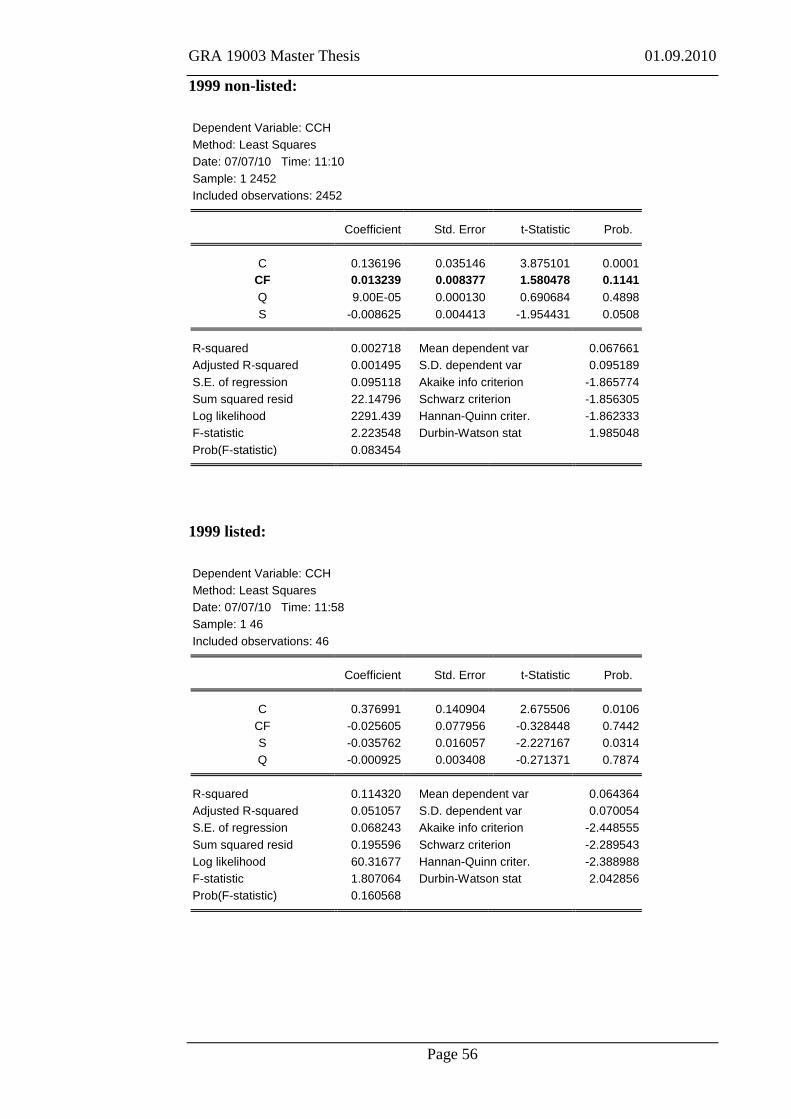
GRA 19003 Master Thesis 01.09.2010
Page 56
1999 non-listed:
Dependent Variable: CCH
Method: Least Squares
Date: 07/07/10 Time: 11:10
Sample: 1 2452
Included observations: 2452 Coefficient Std. Error t-Statistic Prob.
C 0.136196 0.035146 3.875101 0.0001
CF 0.013239 0.008377 1.580478 0.1141
Q 9.00E-05 0.000130 0.690684 0.4898
S -0.008625 0.004413 -1.954431 0.0508
R-squared 0.002718 Mean dependent var 0.067661
Adjusted R-squared 0.001495 S.D. dependent var 0.095189
S.E. of regression 0.095118 Akaike info criterion -1.865774
Sum squared resid 22.14796 Schwarz criterion -1.856305
Log likelihood 2291.439 Hannan-Quinn criter. -1.862333
F-statistic 2.223548 Durbin-Watson stat 1.985048
Prob(F-statistic) 0.083454
1999 listed:
Dependent Variable: CCH
Method: Least Squares
Date: 07/07/10 Time: 11:58
Sample: 1 46
Included observations: 46 Coefficient Std. Error t-Statistic Prob.
C 0.376991 0.140904 2.675506 0.0106
CF -0.025605 0.077956 -0.328448 0.7442
S -0.035762 0.016057 -2.227167 0.0314
Q -0.000925 0.003408 -0.271371 0.7874
R-squared 0.114320 Mean dependent var 0.064364
Adjusted R-squared 0.051057 S.D. dependent var 0.070054
S.E. of regression 0.068243 Akaike info criterion -2.448555
Sum squared resid 0.195596 Schwarz criterion -2.289543
Log likelihood 60.31677 Hannan-Quinn criter. -2.388988
F-statistic 1.807064 Durbin-Watson stat 2.042856
Prob(F-statistic) 0.160568

GRA 19003 Master Thesis 01.09.2010
Page 57
2000 non-listed:
Dependent Variable: CCH
Method: Least Squares
Date: 07/07/10 Time: 11:12
Sample: 1 1205
Included observations: 1205 Coefficient Std. Error t-Statistic Prob.
C 0.002756 0.067779 0.040665 0.9676
CF 0.004762 0.012046 0.395277 0.6927
Q -0.000209 0.000289 -0.725219 0.4685
S 0.010301 0.008604 1.197149 0.2315
R-squared 0.001756 Mean dependent var 0.083422
Adjusted R-squared -0.000738 S.D. dependent var 0.112687
S.E. of regression 0.112729 Akaike info criterion -1.524351
Sum squared resid 15.26203 Schwarz criterion -1.507441
Log likelihood 922.4214 Hannan-Quinn criter. -1.517982
F-statistic 0.704035 Durbin-Watson stat 1.966024
Prob(F-statistic) 0.549665
2000 listed:
Dependent Variable: CCH
Method: Least Squares
Date: 07/07/10 Time: 12:00
Sample: 1 5
Included observations: 5 Coefficient Std. Error t-Statistic Prob.
C -2.904541 0.532934 -5.450093 0.1155
CF -0.944573 0.142876 -6.611127 0.0956
Q -0.238117 0.036212 -6.575640 0.0961
S 0.375245 0.063957 5.867173 0.1075
R-squared 0.987530 Mean dependent var 0.065769
Adjusted R-squared 0.950120 S.D. dependent var 0.065436
S.E. of regression 0.014614 Akaike info criterion -5.623056
Sum squared resid 0.000214 Schwarz criterion -5.935505
Log likelihood 18.05764 Hannan-Quinn criter. -6.461640
F-statistic 26.39727 Durbin-Watson stat 1.971819
Prob(F-statistic) 0.141886

GRA 19003 Master Thesis 01.09.2010
Page 58
2001 non-listed:
Dependent Variable: CCH
Method: Least Squares
Date: 07/07/10 Time: 11:14
Sample: 1 976
Included observations: 975 Coefficient Std. Error t-Statistic Prob.
C 0.152317 0.071852 2.119879 0.0343
CF -0.016209 0.009594 -1.689529 0.0914
Q -9.04E-05 0.000289 -0.313230 0.7542
S -0.009591 0.009134 -1.050078 0.2939
R-squared 0.004366 Mean dependent var 0.077510
Adjusted R-squared 0.001289 S.D. dependent var 0.101186
S.E. of regression 0.101121 Akaike info criterion -1.740903
Sum squared resid 9.928922 Schwarz criterion -1.720873
Log likelihood 852.6904 Hannan-Quinn criter. -1.733281
F-statistic 1.419178 Durbin-Watson stat 2.007125
Prob(F-statistic) 0.235663
2001 listed:
Dependent Variable: CCH
Method: Least Squares
Date: 07/07/10 Time: 12:09
Sample: 1 5
Included observations: 5 Coefficient Std. Error t-Statistic Prob.
C -38.45499 5.875689 -6.544762 0.0965
CF -4.500299 0.693797 -6.486474 0.0974
Q -4.187223 0.658735 -6.356464 0.0993
S 4.756258 0.725715 6.553894 0.0964
R-squared 0.997470 Mean dependent var 0.152852
Adjusted R-squared 0.989879 S.D. dependent var 0.087865
S.E. of regression 0.008839 Akaike info criterion -6.628613
Sum squared resid 7.81E-05 Schwarz criterion -6.941063
Log likelihood 20.57153 Hannan-Quinn criter. -7.467198
F-statistic 131.4065 Durbin-Watson stat 2.231496
Prob(F-statistic) 0.064019

GRA 19003 Master Thesis 01.09.2010
Page 59
2002 non-listed:
Dependent Variable: CCH
Method: Least Squares
Date: 07/07/10 Time: 11:16
Sample: 1 970
Included observations: 970 Coefficient Std. Error t-Statistic Prob.
C 0.185156 0.071450 2.591394 0.0097
CF 0.021243 0.011666 1.820962 0.0689
Q -1.55E-07 2.23E-07 -0.695721 0.4868
S -0.013910 0.009057 -1.535952 0.1249
R-squared 0.006102 Mean dependent var 0.075231
Adjusted R-squared 0.003016 S.D. dependent var 0.103135
S.E. of regression 0.102979 Akaike info criterion -1.704470
Sum squared resid 10.24410 Schwarz criterion -1.684357
Log likelihood 830.6678 Hannan-Quinn criter. -1.696814
F-statistic 1.976958 Durbin-Watson stat 2.000475
Prob(F-statistic) 0.115779
2002 listed cannot be estimated

GRA 19003 Master Thesis 01.09.2010
Page 60
2003 non-listed:
Dependent Variable: CCH
Method: Least Squares
Date: 07/07/10 Time: 11:18
Sample: 1 1143
Included observations: 1142 Coefficient Std. Error t-Statistic Prob.
C 0.257429 0.060567 4.250287 0.0000
CF 0.014210 0.010737 1.323393 0.1860
Q -0.000200 0.000310 -0.644723 0.5192
S -0.023016 0.007688 -2.993857 0.0028
R-squared 0.009713 Mean dependent var 0.075826
Adjusted R-squared 0.007103 S.D. dependent var 0.095290
S.E. of regression 0.094951 Akaike info criterion -1.867418
Sum squared resid 10.25983 Schwarz criterion -1.849763
Log likelihood 1070.296 Hannan-Quinn criter. -1.860751
F-statistic 3.720651 Durbin-Watson stat 1.990712
Prob(F-statistic) 0.011133
2003 listed: (too few observations)
Dependent Variable: CCH
Method: Least Squares
Date: 07/07/10 Time: 12:11
Sample: 1 4
Included observations: 4 Coefficient Std. Error t-Statistic Prob.
C -4.862014 NA NA NA
CF -0.057716 NA NA NA
Q 0.015831 NA NA NA
S 0.605995 NA NA NA
R-squared 1.000000 Mean dependent var 0.156961
S.D. dependent var 0.153660 Sum squared resid 3.52E-27
Durbin-Watson stat 1.625701

GRA 19003 Master Thesis 01.09.2010
Page 61
2004 non-listed:
Dependent Variable: CCH
Method: Least Squares
Date: 07/07/10 Time: 11:20
Sample: 1 1092
Included observations: 1092 Coefficient Std. Error t-Statistic Prob.
C 0.111125 0.066829 1.662838 0.0966
CF 0.015522 0.017602 0.881801 0.3781
Q -0.000245 0.000260 -0.943513 0.3456
S -0.002682 0.008471 -0.316634 0.7516
R-squared 0.001671 Mean dependent var 0.089647
Adjusted R-squared -0.001082 S.D. dependent var 0.109625
S.E. of regression 0.109684 Akaike info criterion -1.578769
Sum squared resid 13.08928 Schwarz criterion -1.560470
Log likelihood 866.0081 Hannan-Quinn criter. -1.571844
F-statistic 0.607002 Durbin-Watson stat 2.002274
Prob(F-statistic) 0.610523
2004 listed:
Dependent Variable: CCH
Method: Least Squares
Date: 07/07/10 Time: 12:12
Sample: 1 5
Included observations: 5 Coefficient Std. Error t-Statistic Prob.
C 0.955608 0.325834 2.932807 0.2092
CF 0.970863 0.323297 3.003009 0.2046
Q 0.006464 0.013658 0.473262 0.7186
S -0.106813 0.039286 -2.718873 0.2244
R-squared 0.961372 Mean dependent var 0.040825
Adjusted R-squared 0.845488 S.D. dependent var 0.040557
S.E. of regression 0.015942 Akaike info criterion -5.449114
Sum squared resid 0.000254 Schwarz criterion -5.761564
Log likelihood 17.62279 Hannan-Quinn criter. -6.287698
F-statistic 8.295982 Durbin-Watson stat 1.947694
Prob(F-statistic) 0.248622

GRA 19003 Master Thesis 01.09.2010
Page 62
Attachment 2
Output: Firms who pay or not pay dividends
1998 (pay dividend):
Dependent Variable: CCH
Method: Least Squares
Date: 07/06/10 Time: 13:44
Sample: 1 515
Included observations: 515 Coefficient Std. Error t-Statistic Prob.
C 0.317035 0.083066 3.816677 0.0002
CF 0.060599 0.032021 1.892477 0.0590
Q -0.000392 0.000466 -0.840629 0.4009
S -0.031035 0.010511 -2.952559 0.0033
R-squared 0.025358 Mean dependent var 0.072509
Adjusted R-squared 0.019636 S.D. dependent var 0.098700
S.E. of regression 0.097726 Akaike info criterion -1.805562
Sum squared resid 4.880235 Schwarz criterion -1.772598
Log likelihood 468.9323 Hannan-Quinn criter. -1.792644
F-statistic 4.431604 Durbin-Watson stat 1.974796
Prob(F-statistic) 0.004348
1998 (not div):
Dependent Variable: CCH
Method: Least Squares
Date: 07/06/10 Time: 14:06
Sample: 1 1540
Included observations: 1539 Coefficient Std. Error t-Statistic Prob.
C 0.091105 0.054111 1.683675 0.0924
CF 0.031698 0.014592 2.172232 0.0300
Q -0.000186 0.000250 -0.744532 0.4567
S -0.002030 0.006805 -0.298346 0.7655
R-squared 0.003479 Mean dependent var 0.074121
Adjusted R-squared 0.001531 S.D. dependent var 0.113300
S.E. of regression 0.113213 Akaike info criterion -1.516498
Sum squared resid 19.67433 Schwarz criterion -1.502622
Log likelihood 1170.945 Hannan-Quinn criter. -1.511336
F-statistic 1.786226 Durbin-Watson stat 2.004890
Prob(F-statistic) 0.147822

GRA 19003 Master Thesis 01.09.2010
Page 63
1999 (pay div):
Dependent Variable: CCH
Method: Least Squares
Date: 07/06/10 Time: 14:11
Sample: 1 831
Included observations: 831 Coefficient Std. Error t-Statistic Prob.
C 0.217691 0.049081 4.435338 0.0000
CF -0.009214 0.015279 -0.603029 0.5467
Q 7.38E-05 0.000118 0.625565 0.5318
S -0.019214 0.006145 -3.126572 0.0018
R-squared 0.012099 Mean dependent var 0.064468
Adjusted R-squared 0.008516 S.D. dependent var 0.083570
S.E. of regression 0.083213 Akaike info criterion -2.130017
Sum squared resid 5.726524 Schwarz criterion -2.107285
Log likelihood 889.0221 Hannan-Quinn criter. -2.121300
F-statistic 3.376223 Durbin-Watson stat 2.058778
Prob(F-statistic) 0.017954
1999 (not div):
Dependent Variable: CCH
Method: Least Squares
Date: 07/06/10 Time: 14:18
Sample: 1 2498
Included observations: 2498 Coefficient Std. Error t-Statistic Prob.
C 0.142215 0.033439 4.253005 0.0000
CF 0.012871 0.008313 1.548358 0.1217
Q 9.01E-05 0.000130 0.694944 0.4872
S -0.009372 0.004191 -2.236384 0.0254
R-squared 0.003102 Mean dependent var 0.067600
Adjusted R-squared 0.001903 S.D. dependent var 0.094777
S.E. of regression 0.094687 Akaike info criterion -1.874889
Sum squared resid 22.36008 Schwarz criterion -1.865564
Log likelihood 2345.736 Hannan-Quinn criter. -1.871504
F-statistic 2.586677 Durbin-Watson stat 2.017139
Prob(F-statistic) 0.051482

GRA 19003 Master Thesis 01.09.2010
Page 64
2000 (pay div):
Dependent Variable: CCH
Method: Least Squares
Date: 07/06/10 Time: 14:22
Sample: 1 388
Included observations: 388 Coefficient Std. Error t-Statistic Prob.
C 0.122710 0.113990 1.076492 0.2824
CF 0.044474 0.035192 1.263756 0.2071
Q 0.000301 0.001900 0.158290 0.8743
S -0.005009 0.014538 -0.344525 0.7306
R-squared 0.004434 Mean dependent var 0.085196
Adjusted R-squared -0.003344 S.D. dependent var 0.106372
S.E. of regression 0.106549 Akaike info criterion -1.630161
Sum squared resid 4.359461 Schwarz criterion -1.589326
Log likelihood 320.2513 Hannan-Quinn criter. -1.613971
F-statistic 0.570075 Durbin-Watson stat 1.847982
Prob(F-statistic) 0.635013
2000 (not div):
Dependent Variable: CCH
Method: Least Squares
Date: 07/06/10 Time: 14:24
Sample: 1 1210
Included observations: 1210 Coefficient Std. Error t-Statistic Prob.
C 0.005629 0.067431 0.083483 0.9335
CF 0.004663 0.012026 0.387710 0.6983
Q -0.000210 0.000288 -0.727311 0.4672
S 0.009923 0.008558 1.159560 0.2465
R-squared 0.001673 Mean dependent var 0.083349
Adjusted R-squared -0.000811 S.D. dependent var 0.112523
S.E. of regression 0.112568 Akaike info criterion -1.527215
Sum squared resid 15.28194 Schwarz criterion -1.510361
Log likelihood 927.9653 Hannan-Quinn criter. -1.520869
F-statistic 0.673600 Durbin-Watson stat 1.964026
Prob(F-statistic) 0.568277

GRA 19003 Master Thesis 01.09.2010
Page 65
2001( pay div):
Dependent Variable: CCH
Method: Least Squares
Date: 07/06/10 Time: 14:56
Sample: 1 335
Included observations: 335 Coefficient Std. Error t-Statistic Prob.
C 0.055700 0.096651 0.576298 0.5648
CF 0.068189 0.029415 2.318149 0.0211
Q 0.007694 0.002870 2.681158 0.0077
S 0.001731 0.012334 0.140358 0.8885
R-squared 0.036838 Mean dependent var 0.075006
Adjusted R-squared 0.028109 S.D. dependent var 0.081443
S.E. of regression 0.080290 Akaike info criterion -2.194482
Sum squared resid 2.133772 Schwarz criterion -2.148940
Log likelihood 371.5757 Hannan-Quinn criter. -2.176325
F-statistic 4.219942 Durbin-Watson stat 2.066298
Prob(F-statistic) 0.006012
2001 (not div):
Dependent Variable: CCH
Method: Least Squares
Date: 07/06/10 Time: 15:01
Sample: 1 981
Included observations: 980 Coefficient Std. Error t-Statistic Prob.
C 0.133466 0.071183 1.874988 0.0611
CF -0.019122 0.009405 -2.033217 0.0423
Q -9.35E-05 0.000289 -0.324093 0.7459
S -0.007163 0.009046 -0.791883 0.4286
R-squared 0.005103 Mean dependent var 0.077895
Adjusted R-squared 0.002045 S.D. dependent var 0.101226
S.E. of regression 0.101123 Akaike info criterion -1.740890
Sum squared resid 9.980387 Schwarz criterion -1.720941
Log likelihood 857.0363 Hannan-Quinn criter. -1.733301
F-statistic 1.668609 Durbin-Watson stat 2.036181
Prob(F-statistic) 0.172120

GRA 19003 Master Thesis 01.09.2010
Page 66
2002 (pay div):
Dependent Variable: CCH
Method: Least Squares
Date: 07/06/10 Time: 15:04
Sample: 1 329
Included observations: 329 Coefficient Std. Error t-Statistic Prob.
C 0.226482 0.116332 1.946870 0.0524
CF 0.099840 0.037395 2.669918 0.0080
Q -1.73E-07 2.24E-07 -0.769490 0.4422
S -0.018651 0.014736 -1.265676 0.2065
R-squared 0.028601 Mean dependent var 0.085218
Adjusted R-squared 0.019634 S.D. dependent var 0.103684
S.E. of regression 0.102661 Akaike info criterion -1.702681
Sum squared resid 3.425280 Schwarz criterion -1.656529
Log likelihood 284.0911 Hannan-Quinn criter. -1.684270
F-statistic 3.189624 Durbin-Watson stat 2.010303
Prob(F-statistic) 0.023922
2002 (not div):
Dependent Variable: CCH
Method: Least Squares
Date: 07/06/10 Time: 15:06
Sample: 1 971
Included observations: 971 Coefficient Std. Error t-Statistic Prob.
C 0.185669 0.071413 2.599938 0.0095
CF 0.021406 0.011656 1.836475 0.0666
Q -1.55E-07 2.23E-07 -0.695380 0.4870
S -0.013982 0.009052 -1.544651 0.1228
R-squared 0.006181 Mean dependent var 0.075174
Adjusted R-squared 0.003097 S.D. dependent var 0.103097
S.E. of regression 0.102937 Akaike info criterion -1.705289
Sum squared resid 10.24635 Schwarz criterion -1.685193
Log likelihood 831.9179 Hannan-Quinn criter. -1.697640
F-statistic 2.004591 Durbin-Watson stat 2.014775
Prob(F-statistic) 0.111696

GRA 19003 Master Thesis 01.09.2010
Page 67
2003 (pay div):
Dependent Variable: CCH
Method: Least Squares
Date: 07/06/10 Time: 15:08
Sample: 1 425
Included observations: 425 Coefficient Std. Error t-Statistic Prob.
C 0.212257 0.084104 2.523757 0.0120
CF 0.042032 0.025475 1.649915 0.0997
Q 0.001784 0.001514 1.178578 0.2392
S -0.017110 0.010704 -1.598438 0.1107
R-squared 0.015303 Mean dependent var 0.080811
Adjusted R-squared 0.008286 S.D. dependent var 0.083581
S.E. of regression 0.083234 Akaike info criterion -2.124965
Sum squared resid 2.916616 Schwarz criterion -2.086827
Log likelihood 455.5550 Hannan-Quinn criter. -2.109898
F-statistic 2.180915 Durbin-Watson stat 1.954674
Prob(F-statistic) 0.089658
2003 (not div):
Dependent Variable: CCH
Method: Least Squares
Date: 07/06/10 Time: 15:11
Sample: 1 1147
Included observations: 1146 Coefficient Std. Error t-Statistic Prob.
C 0.244068 0.060631 4.025456 0.0001
CF 0.014541 0.010759 1.351550 0.1768
Q -0.000201 0.000311 -0.646521 0.5181
S -0.021277 0.007695 -2.765202 0.0058
R-squared 0.008617 Mean dependent var 0.076109
Adjusted R-squared 0.006013 S.D. dependent var 0.095568
S.E. of regression 0.095280 Akaike info criterion -1.860507
Sum squared resid 10.36742 Schwarz criterion -1.842901
Log likelihood 1070.070 Hannan-Quinn criter. -1.853860
F-statistic 3.308756 Durbin-Watson stat 1.895184
Prob(F-statistic) 0.019545

GRA 19003 Master Thesis 01.09.2010
Page 68
2004 (pay div):
Dependent Variable: CCH
Method: Least Squares
Date: 07/06/10 Time: 15:14
Sample: 1 457
Included observations: 457 Coefficient Std. Error t-Statistic Prob.
C 0.035862 0.093372 0.384073 0.7011
CF 0.020470 0.034526 0.592903 0.5535
Q -0.000171 0.000292 -0.584974 0.5589
S 0.006275 0.011902 0.527174 0.5983
R-squared 0.002176 Mean dependent var 0.085375
Adjusted R-squared -0.004432 S.D. dependent var 0.098927
S.E. of regression 0.099146 Akaike info criterion -1.775732
Sum squared resid 4.452959 Schwarz criterion -1.739630
Log likelihood 409.7548 Hannan-Quinn criter. -1.761512
F-statistic 0.329275 Durbin-Watson stat 1.979518
Prob(F-statistic) 0.804195
2004 (not div):
Dependent Variable: CCH
Method: Least Squares
Date: 07/06/10 Time: 15:20
Sample: 1 640
Included observations: 640 Coefficient Std. Error t-Statistic Prob.
C 0.186688 0.093069 2.005922 0.0453
CF 0.018609 0.021403 0.869471 0.3849
Q -0.000347 0.000464 -0.747480 0.4551
S -0.011817 0.011745 -1.006115 0.3147
R-squared 0.003795 Mean dependent var 0.092316
Adjusted R-squared -0.000905 S.D. dependent var 0.116375
S.E. of regression 0.116428 Akaike info criterion -1.456858
Sum squared resid 8.621276 Schwarz criterion -1.428974
Log likelihood 470.1946 Hannan-Quinn criter. -1.446035
F-statistic 0.807510 Durbin-Watson stat 2.023084
Prob(F-statistic) 0.489955

GRA 19003 Master Thesis 01.09.2010
Page 69
Attachment 3
Output: comparing the 20% smallest and 20 % largest firms
1998 20% largest
Dependent Variable: CCH
Method: Least Squares
Date: 07/12/10 Time: 13:32
Sample: 1 6978
Included observations: 6978 Coefficient Std. Error t-Statistic Prob.
C 0.685232 0.066122 10.36317 0.0000
CF 0.003991 0.005621 0.709979 0.4777
Q 6.05E-05 0.000285 0.212420 0.8318
S -0.097088 0.011863 -8.184303 0.0000
R-squared 0.009539 Mean dependent var 0.144843
Adjusted R-squared 0.009113 S.D. dependent var 0.244753
S.E. of regression 0.243635 Akaike info criterion 0.014286
Sum squared resid 413.9643 Schwarz criterion 0.018213
Log likelihood -45.84257 Hannan-Quinn criter. 0.015639
F-statistic 22.38916 Durbin-Watson stat 1.970424
Prob(F-statistic) 0.000000
1998 20% smallest
Dependent Variable: CCH
Method: Least Squares
Date: 07/12/10 Time: 13:39
Sample: 1 6979
Included observations: 6978 Coefficient Std. Error t-Statistic Prob.
C 0.125323 0.021193 5.913572 0.0000
CF 0.018277 0.005773 3.165826 0.0016
Q -1.86E-05 7.56E-05 -0.246038 0.8057
S -0.006353 0.002912 -2.181884 0.0292
R-squared 0.002194 Mean dependent var 0.078981
Adjusted R-squared 0.001765 S.D. dependent var 0.107621
S.E. of regression 0.107526 Akaike info criterion -1.621594
Sum squared resid 80.63240 Schwarz criterion -1.617667
Log likelihood 5661.740 Hannan-Quinn criter. -1.620240
F-statistic 5.111323 Durbin-Watson stat 1.980138
Prob(F-statistic) 0.001564

GRA 19003 Master Thesis 01.09.2010
Page 70
1999 20% largest
Dependent Variable: CCH
Method: Least Squares
Date: 07/12/10 Time: 13:45
Sample: 1 8603
Included observations: 8603 Coefficient Std. Error t-Statistic Prob.
C 0.543886 0.034239 15.88483 0.0000
CF -0.001323 0.001079 -1.225376 0.2205
Q 2.04E-05 0.000182 0.111843 0.9110
S -0.072917 0.006124 -11.90605 0.0000
R-squared 0.016775 Mean dependent var 0.136832
Adjusted R-squared 0.016432 S.D. dependent var 0.142111
S.E. of regression 0.140939 Akaike info criterion -1.080515
Sum squared resid 170.8087 Schwarz criterion -1.077233
Log likelihood 4651.836 Hannan-Quinn criter. -1.079396
F-statistic 48.90433 Durbin-Watson stat 1.992090
Prob(F-statistic) 0.000000
1999 20% smallest:
Dependent Variable: CCH
Method: Least Squares
Date: 07/12/10 Time: 13:50
Sample: 1 8604
Included observations: 8604 Coefficient Std. Error t-Statistic Prob.
C 0.166290 0.017658 9.417042 0.0000
CF 0.012805 0.004860 2.634950 0.0084
Q -3.53E-07 4.70E-05 -0.007515 0.9940
S -0.012221 0.002388 -5.118143 0.0000
R-squared 0.003907 Mean dependent var 0.076147
Adjusted R-squared 0.003559 S.D. dependent var 0.104023
S.E. of regression 0.103838 Akaike info criterion -1.691506
Sum squared resid 92.72789 Schwarz criterion -1.688224
Log likelihood 7280.860 Hannan-Quinn criter. -1.690387
F-statistic 11.24353 Durbin-Watson stat 1.997943
Prob(F-statistic) 0.000000

GRA 19003 Master Thesis 01.09.2010
Page 71
2000 20% largest:
Dependent Variable: CCH
Method: Least Squares
Date: 07/13/10 Time: 10:47
Sample: 1 7631
Included observations: 7631 Coefficient Std. Error t-Statistic Prob.
C 0.719405 0.039692 18.12476 0.0000
CF -0.008353 0.002477 -3.372161 0.0007
Q -0.000141 0.000171 -0.827321 0.4081
S -0.103710 0.007141 -14.52365 0.0000
R-squared 0.029530 Mean dependent var 0.144436
Adjusted R-squared 0.029148 S.D. dependent var 0.155715
S.E. of regression 0.153429 Akaike info criterion -0.910634
Sum squared resid 179.5430 Schwarz criterion -0.906996
Log likelihood 3478.525 Hannan-Quinn criter. -0.909386
F-statistic 77.35959 Durbin-Watson stat 1.942705
Prob(F-statistic) 0.000000
2000 20% smallest:
Dependent Variable: CCH
Method: Least Squares
Date: 07/13/10 Time: 11:04
Sample: 1 7633
Included observations: 7633 Coefficient Std. Error t-Statistic Prob.
C 0.050403 0.022507 2.239433 0.0252
CF -0.002886 0.004740 -0.608790 0.5427
Q -2.13E-05 5.77E-05 -0.368961 0.7122
S 0.004563 0.003138 1.454043 0.1460
R-squared 0.000352 Mean dependent var 0.083126
Adjusted R-squared -0.000041 S.D. dependent var 0.105967
S.E. of regression 0.105969 Akaike info criterion -1.650808
Sum squared resid 85.67003 Schwarz criterion -1.647171
Log likelihood 6304.309 Hannan-Quinn criter. -1.649560
F-statistic 0.895435 Durbin-Watson stat 1.973398
Prob(F-statistic) 0.442610

GRA 19003 Master Thesis 01.09.2010
Page 72
2001 20 % smallest:
Dependent Variable: CCH
Method: Least Squares
Date: 07/13/10 Time: 11:10
Sample: 1 7636
Included observations: 7636 Coefficient Std. Error t-Statistic Prob.
CF -0.007139 0.003483 -2.049636 0.0404
C 0.607432 0.070297 8.640965 0.0000
Q -0.000250 0.000438 -0.571772 0.5675
S -0.083616 0.012617 -6.627182 0.0000
R-squared 0.006917 Mean dependent var 0.142960
Adjusted R-squared 0.006526 S.D. dependent var 0.270610
S.E. of regression 0.269726 Akaike info criterion 0.217703
Sum squared resid 555.2437 Schwarz criterion 0.221338
Log likelihood -827.1886 Hannan-Quinn criter. 0.218950
F-statistic 17.71898 Durbin-Watson stat 2.004581
Prob(F-statistic) 0.000000
2001 20% largest:
Dependent Variable: CCH
Method: Least Squares
Date: 07/13/10 Time: 11:26
Sample: 1 7638
Included observations: 7637 Coefficient Std. Error t-Statistic Prob.
C 0.170523 0.022786 7.483809 0.0000
CF -0.009433 0.004153 -2.271454 0.0231
Q 9.43E-07 4.35E-05 0.021654 0.9827
S -0.012041 0.003211 -3.749649 0.0002
R-squared 0.002433 Mean dependent var 0.085316
Adjusted R-squared 0.002041 S.D. dependent var 0.105458
S.E. of regression 0.105351 Akaike info criterion -1.662523
Sum squared resid 84.71665 Schwarz criterion -1.658888
Log likelihood 6352.345 Hannan-Quinn criter. -1.661276
F-statistic 6.205451 Durbin-Watson stat 1.957935
Prob(F-statistic) 0.000332

GRA 19003 Master Thesis 01.09.2010
Page 73
2002 20% largest:
Dependent Variable: CCH
Method: Least Squares
Date: 07/13/10 Time: 11:26
Sample: 1 7638
Included observations: 7637 Coefficient Std. Error t-Statistic Prob.
C 0.170523 0.022786 7.483809 0.0000
CF -0.009433 0.004153 -2.271454 0.0231
Q 9.43E-07 4.35E-05 0.021654 0.9827
S -0.012041 0.003211 -3.749649 0.0002
R-squared 0.002433 Mean dependent var 0.085316
Adjusted R-squared 0.002041 S.D. dependent var 0.105458
S.E. of regression 0.105351 Akaike info criterion -1.662523
Sum squared resid 84.71665 Schwarz criterion -1.658888
Log likelihood 6352.345 Hannan-Quinn criter. -1.661276
F-statistic 6.205451 Durbin-Watson stat 1.957935
Prob(F-statistic) 0.000332
2002 20% smallest:
Dependent Variable: CCH
Method: Least Squares
Date: 07/13/10 Time: 11:35
Sample: 1 6734
Included observations: 6734 Coefficient Std. Error t-Statistic Prob.
C 0.170633 0.022977 7.426229 0.0000
CF 0.020637 0.004853 4.252604 0.0000
Q 0.000101 8.29E-05 1.217456 0.2235
S -0.012006 0.003218 -3.730458 0.0002
R-squared 0.004960 Mean dependent var 0.085217
Adjusted R-squared 0.004517 S.D. dependent var 0.101661
S.E. of regression 0.101431 Akaike info criterion -1.738275
Sum squared resid 69.24038 Schwarz criterion -1.734227
Log likelihood 5856.773 Hannan-Quinn criter. -1.736878
F-statistic 11.18262 Durbin-Watson stat 2.003829
Prob(F-statistic) 0.000000

GRA 19003 Master Thesis 01.09.2010
Page 74
2003 20% largest:
Dependent Variable: CCH
Method: Least Squares
Date: 07/13/10 Time: 11:46
Sample: 1 7736
Included observations: 7736 Coefficient Std. Error t-Statistic Prob.
C 0.670846 0.046216 14.51554 0.0000
CF -0.016001 0.003020 -5.298396 0.0000
Q -0.000453 0.000293 -1.547864 0.1217
S -0.095129 0.008271 -11.50192 0.0000
R-squared 0.023435 Mean dependent var 0.141811
Adjusted R-squared 0.023056 S.D. dependent var 0.173771
S.E. of regression 0.171756 Akaike info criterion -0.684964
Sum squared resid 228.0957 Schwarz criterion -0.681368
Log likelihood 2653.440 Hannan-Quinn criter. -0.683731
F-statistic 61.84900 Durbin-Watson stat 1.994622
Prob(F-statistic) 0.000000
2003 20% smallest:
Dependent Variable: CCH
Method: Least Squares
Date: 07/13/10 Time: 11:51
Sample: 1 7737
Included observations: 7736 Coefficient Std. Error t-Statistic Prob.
C 0.166398 0.022202 7.494801 0.0000
CF 0.004439 0.004208 1.054944 0.2915
Q 3.93E-05 6.28E-05 0.625868 0.5314
S -0.011443 0.003100 -3.691030 0.0002
R-squared 0.001979 Mean dependent var 0.084644
Adjusted R-squared 0.001592 S.D. dependent var 0.102681
S.E. of regression 0.102600 Akaike info criterion -1.715450
Sum squared resid 81.39217 Schwarz criterion -1.711854
Log likelihood 6639.360 Hannan-Quinn criter. -1.714217
F-statistic 5.110925 Durbin-Watson stat 2.007677
Prob(F-statistic) 0.001564

GRA 19003 Master Thesis 01.09.2010
Page 75
2004 20 % largest:
Dependent Variable: CCH
Method: Least Squares
Date: 07/13/10 Time: 11:58
Sample: 1 5976
Included observations: 5975 Coefficient Std. Error t-Statistic Prob.
C 0.771308 0.048633 15.85991 0.0000
CF -0.008088 0.003239 -2.497470 0.0125
Q 4.88E-05 0.000243 0.201163 0.8406
S -0.108570 0.008608 -12.61244 0.0000
R-squared 0.028371 Mean dependent var 0.159315
Adjusted R-squared 0.027883 S.D. dependent var 0.162989
S.E. of regression 0.160701 Akaike info criterion -0.817878
Sum squared resid 154.1992 Schwarz criterion -0.813396
Log likelihood 2447.410 Hannan-Quinn criter. -0.816321
F-statistic 58.11744 Durbin-Watson stat 1.965144
Prob(F-statistic) 0.000000
2004 20% smallest:
Dependent Variable: CCH
Method: Least Squares
Date: 07/13/10 Time: 12:03
Sample: 1 5978
Included observations: 5978 Coefficient Std. Error t-Statistic Prob.
C 0.174775 0.027401 6.378494 0.0000
CF 0.040181 0.007062 5.689950 0.0000
Q -3.26E-05 6.19E-05 -0.525610 0.5992
S -0.010647 0.003785 -2.813351 0.0049
R-squared 0.007138 Mean dependent var 0.098523
Adjusted R-squared 0.006640 S.D. dependent var 0.113552
S.E. of regression 0.113175 Akaike info criterion -1.519101
Sum squared resid 76.51792 Schwarz criterion -1.514621
Log likelihood 4544.593 Hannan-Quinn criter. -1.517545
F-statistic 14.31654 Durbin-Watson stat 1.988703
Prob(F-statistic) 0.000000

GRA 19003 Master Thesis 01.09.2010
Page 76
Attachment 4
KZ-output
Average KZ-index number for the listed and non-listed firms for each year:
1998 non-listed: 1,448377
1998 listed: 1,335138
1999 non-listed: 1,268063
1999 listed: 0,464471
2000 non-listed: 1,349688
2000 listed: 0,888664
2001 non-listed: 0,509318
2001 listed: 1,554391
2002 non- listed: 253,5427
2002 listed: (1 firm): 1,010423
2003 non-listed: 0,583543
2003 listed: -0,93931
2004 non-listed(5 firms): 0,091984
2004 listed: 0,245609

GRA 19003 Master Thesis 01.09.2010
Page 77
Attachment 5
Output from independent sample t-test.
Testing whether the difference in average KZ-index number is
significant.
Group Statistics
firmtype N Mean Std. Deviation Std. Error Mean
KZ 1 6 .873194 .5530792 .2257937
2 6 .591494 .8997354 .3673155
(1= non-listed, 2=listed firms)
Independent Samples Test
Levene's Test for
Equality of
Variances t-test for Equality of Means
F Sig. t df
Sig.
(2-
tailed)
Mean
Difference
Std. Error
Difference
95% Confidence Interval
of the Difference
Lower Upper
KZ Equal variances
assumed
.706 .420 .653 10 .528 .2817005 .4311652 -.6789954 1.2423964
Equal variances
not assumed
.653 8.307 .531 .2817005 .4311652 -.7062167 1.2696177

GRA 19003 Master Thesis 01.09.2010
Page 78
Attachment 6
KZ-index
Average debt for top 20% and bottom 20% in terms of the KZ-index value.
1998
Bottom: 0,477608
Top: 0,907244
1999
Bottom: 0,0015
Top: 0,6563
2000
Bottom: 0,458212
Top: 0,954039
2001
Bottom: 0,578216
Top: 0,977288
2002
Bottom: 0,512002
Top: 0,649048
2003:
Bottom: 0,636005
Top: 0,920935
2004:
Bottom: 0,709898
Top: 0,911527

GRA 19003 Master Thesis 01.09.2010
Page 79
Attachment 7
Output for the independent sample t-test.
Testing whether the difference in leverage among the firms with the top and
bottom 20 % KZ-index numbers are significantly different.
H0: means are equal
H1: means are unequal
Group Statistics
highlow N Mean Std. Deviation
Std. Error
Mean
leverage 1 7 .853769 .1395962 .0527624
2 7 .481920 .2299558 .0869151
Independent Samples Test
Levene's Test for
Equality of
Variances t-test for Equality of Means
F Sig. t df
Sig. (2-
tailed)
Mean
Differen
ce
Std.
Error
Differen
ce
95% Confidence
Interval of the
Difference
Lower Upper
levera
ge
Equal variances
assumed
.199 .663 3.657 12 .003 .3718486 .1016765 .1503145 .5933826
Equal variances
not assumed
3.657 9.893 .004 .3718486 .1016765 .1449681 .5987290

GRA 19003 Master Thesis 01.09.2010
Page 80
Attachment 8
Output for testing the change in cash holdings for firms with
the top and bottom 20 % of leverage.
1998 bottom 20 %:
Dependent Variable: CCH
Method: Least Squares
Date: 08/03/10 Time: 14:42
Sample: 1 308
Included observations: 308 Coefficient Std. Error t-Statistic Prob.
C 0.280448 0.115879 2.420188 0.0161
CF -0.025443 0.058534 -0.434678 0.6641
Q 0.001099 0.001382 0.795315 0.4271
S -0.023671 0.014575 -1.624066 0.1054
R-squared 0.011044 Mean dependent var 0.093787
Adjusted R-squared 0.001285 S.D. dependent var 0.115466
S.E. of regression 0.115392 Akaike info criterion -1.468069
Sum squared resid 4.047825 Schwarz criterion -1.419626
Log likelihood 230.0826 Hannan-Quinn criter. -1.448699
F-statistic 1.131626 Durbin-Watson stat 1.529994
Prob(F-statistic) 0.336445
1998 top 20 %:
Dependent Variable: CCH
Method: Least Squares
Date: 08/03/10 Time: 14:43
Sample: 1 308
Included observations: 308 Coefficient Std. Error t-Statistic Prob.
C -0.019620 0.151523 -0.129482 0.8971
CF 0.011420 0.029564 0.386278 0.6996
Q -0.000236 0.000332 -0.709389 0.4786
S 0.012149 0.019144 0.634607 0.5262
R-squared 0.003032 Mean dependent var 0.075276
Adjusted R-squared -0.006806 S.D. dependent var 0.128678
S.E. of regression 0.129116 Akaike info criterion -1.243316
Sum squared resid 5.067932 Schwarz criterion -1.194873
Log likelihood 195.4706 Hannan-Quinn criter. -1.223946
F-statistic 0.308206 Durbin-Watson stat 2.130925
Prob(F-statistic) 0.819456

GRA 19003 Master Thesis 01.09.2010
Page 81
1999 bottom 20 %:
Dependent Variable: CCH
Method: Least Squares
Date: 08/03/10 Time: 14:44
Sample: 1 500
Included observations: 500 Coefficient Std. Error t-Statistic Prob.
C 0.169091 0.084402 2.003397 0.0457
CF 0.009949 0.023263 0.427693 0.6691
Q -0.000106 0.000700 -0.151323 0.8798
S -0.010165 0.010509 -0.967248 0.3339
R-squared 0.002419 Mean dependent var 0.087463
Adjusted R-squared -0.003615 S.D. dependent var 0.117250
S.E. of regression 0.117462 Akaike info criterion -1.437440
Sum squared resid 6.843440 Schwarz criterion -1.403724
Log likelihood 363.3601 Hannan-Quinn criter. -1.424210
F-statistic 0.400941 Durbin-Watson stat 2.090190
Prob(F-statistic) 0.752386
1999 top 20 %:
Dependent Variable: CCH
Method: Least Squares
Date: 08/03/10 Time: 14:45
Sample: 1 500
Included observations: 500 Coefficient Std. Error t-Statistic Prob.
C 0.163249 0.088909 1.836142 0.0669
CF 0.015094 0.015231 0.991003 0.3222
Q -0.000108 0.002743 -0.039315 0.9687
S -0.012754 0.011239 -1.134745 0.2570
R-squared 0.004476 Mean dependent var 0.061672
Adjusted R-squared -0.001545 S.D. dependent var 0.096872
S.E. of regression 0.096947 Akaike info criterion -1.821336
Sum squared resid 4.661769 Schwarz criterion -1.787619
Log likelihood 459.3340 Hannan-Quinn criter. -1.808106
F-statistic 0.743378 Durbin-Watson stat 1.957031
Prob(F-statistic) 0.526576

GRA 19003 Master Thesis 01.09.2010
Page 82
2000 bottom 20 %:
Dependent Variable: CCH
Method: Least Squares
Date: 08/03/10 Time: 14:46
Sample: 1 242
Included observations: 242 Coefficient Std. Error t-Statistic Prob.
C 0.116904 0.165096 0.708098 0.4796
CF -0.008872 0.037024 -0.239627 0.8108
Q 0.001026 0.001119 0.916420 0.3604
S -0.001448 0.020909 -0.069275 0.9448
R-squared 0.003857 Mean dependent var 0.106936
Adjusted R-squared -0.008699 S.D. dependent var 0.126988
S.E. of regression 0.127539 Akaike info criterion -1.264396
Sum squared resid 3.871364 Schwarz criterion -1.206728
Log likelihood 156.9919 Hannan-Quinn criter. -1.241165
F-statistic 0.307173 Durbin-Watson stat 2.072968
Prob(F-statistic) 0.820196
2000 top 20 %:
Dependent Variable: CCH
Method: Least Squares
Date: 08/03/10 Time: 14:47
Sample: 1 242
Included observations: 242 Coefficient Std. Error t-Statistic Prob.
C -0.274394 0.164857 -1.664437 0.0973
CF -0.004381 0.019448 -0.225261 0.8220
Q -0.000348 0.000629 -0.553911 0.5802
S 0.045572 0.020945 2.175768 0.0306
R-squared 0.022208 Mean dependent var 0.084436
Adjusted R-squared 0.009883 S.D. dependent var 0.124274
S.E. of regression 0.123658 Akaike info criterion -1.326202
Sum squared resid 3.639336 Schwarz criterion -1.268533
Log likelihood 164.4704 Hannan-Quinn criter. -1.302971
F-statistic 1.801843 Durbin-Watson stat 2.231892
Prob(F-statistic) 0.147494

GRA 19003 Master Thesis 01.09.2010
Page 83
2001, bottom 20%:
Dependent Variable: CCH
Method: Least Squares
Date: 08/03/10 Time: 14:48
Sample: 1 196
Included observations: 196 Coefficient Std. Error t-Statistic Prob.
C 0.091352 0.168386 0.542512 0.5881
CF -0.084337 0.037716 -2.236110 0.0265
Q -0.000592 0.000655 -0.903235 0.3675
S -0.000782 0.021296 -0.036735 0.9707
R-squared 0.027805 Mean dependent var 0.087914
Adjusted R-squared 0.012615 S.D. dependent var 0.118627
S.E. of regression 0.117876 Akaike info criterion -1.418163
Sum squared resid 2.667811 Schwarz criterion -1.351263
Log likelihood 142.9800 Hannan-Quinn criter. -1.391079
F-statistic 1.830427 Durbin-Watson stat 1.934507
Prob(F-statistic) 0.142993
2001, top 20%:
Dependent Variable: CCH
Method: Least Squares
Date: 08/03/10 Time: 14:49
Sample: 1 196
Included observations: 196 Coefficient Std. Error t-Statistic Prob.
C 0.136992 0.214733 0.637963 0.5243
CF -0.021233 0.037198 -0.570820 0.5688
Q -3.99E-05 0.000394 -0.101242 0.9195
S -0.007420 0.027536 -0.269477 0.7879
R-squared 0.002025 Mean dependent var 0.080514
Adjusted R-squared -0.013568 S.D. dependent var 0.113709
S.E. of regression 0.114477 Akaike info criterion -1.476681
Sum squared resid 2.516177 Schwarz criterion -1.409780
Log likelihood 148.7147 Hannan-Quinn criter. -1.449596
F-statistic 0.129877 Durbin-Watson stat 2.009195
Prob(F-statistic) 0.942250

GRA 19003 Master Thesis 01.09.2010
Page 84
2002, bottom 20 %:
Dependent Variable: CCH
Method: Least Squares
Date: 08/03/10 Time: 14:51
Sample: 1 194
Included observations: 194 Coefficient Std. Error t-Statistic Prob.
C 0.325856 0.181728 1.793101 0.0745
CF -0.007367 0.030092 -0.244819 0.8069
Q -3.07E-07 1.62E-06 -0.189534 0.8499
S -0.029008 0.022906 -1.266420 0.2069
R-squared 0.009185 Mean dependent var 0.095470
Adjusted R-squared -0.006460 S.D. dependent var 0.132915
S.E. of regression 0.133343 Akaike info criterion -1.171379
Sum squared resid 3.378275 Schwarz criterion -1.104000
Log likelihood 117.6238 Hannan-Quinn criter. -1.144095
F-statistic 0.587104 Durbin-Watson stat 1.884901
Prob(F-statistic) 0.624161
2002, top 20%:
Dependent Variable: CCH
Method: Least Squares
Date: 08/03/10 Time: 14:52
Sample: 1 194
Included observations: 194 Coefficient Std. Error t-Statistic Prob.
C -0.212978 0.207661 -1.025605 0.3064
CF -0.008050 0.035456 -0.227047 0.8206
Q -1.16E-07 2.54E-07 -0.457967 0.6475
S 0.036613 0.026499 1.381683 0.1687
R-squared 0.011904 Mean dependent var 0.073686
Adjusted R-squared -0.003697 S.D. dependent var 0.114312
S.E. of regression 0.114523 Akaike info criterion -1.475674
Sum squared resid 2.491961 Schwarz criterion -1.408295
Log likelihood 147.1404 Hannan-Quinn criter. -1.448391
F-statistic 0.763018 Durbin-Watson stat 1.992314
Prob(F-statistic) 0.516104

GRA 19003 Master Thesis 01.09.2010
Page 85
2003, bottom 20%:
Dependent Variable: CCH
Method: Least Squares
Date: 08/03/10 Time: 14:53
Sample: 1 229
Included observations: 229 Coefficient Std. Error t-Statistic Prob.
C 0.364598 0.141577 2.575262 0.0107
CF -0.039845 0.042948 -0.927749 0.3545
Q -0.000284 0.000484 -0.588283 0.5569
S -0.033865 0.017794 -1.903206 0.0583
R-squared 0.020746 Mean dependent var 0.095233
Adjusted R-squared 0.007690 S.D. dependent var 0.122290
S.E. of regression 0.121818 Akaike info criterion -1.355257
Sum squared resid 3.338940 Schwarz criterion -1.295279
Log likelihood 159.1769 Hannan-Quinn criter. -1.331061
F-statistic 1.588942 Durbin-Watson stat 2.109118
Prob(F-statistic) 0.192875
2003, top 20%:
Dependent Variable: CCH
Method: Least Squares
Date: 08/03/10 Time: 14:54
Sample: 1 229
Included observations: 229 Coefficient Std. Error t-Statistic Prob.
C 0.145174 0.129807 1.118381 0.2646
CF 0.016474 0.021170 0.778191 0.4373
Q -0.000507 0.000485 -1.044151 0.2975
S -0.010677 0.016629 -0.642065 0.5215
R-squared 0.008568 Mean dependent var 0.060409
Adjusted R-squared -0.004651 S.D. dependent var 0.077737
S.E. of regression 0.077917 Akaike info criterion -2.249030
Sum squared resid 1.365992 Schwarz criterion -2.189052
Log likelihood 261.5139 Hannan-Quinn criter. -2.224833
F-statistic 0.648128 Durbin-Watson stat 2.138251
Prob(F-statistic) 0.584885

GRA 19003 Master Thesis 01.09.2010
Page 86
2004, bottom 20 %:
Dependent Variable: CCH
Method: Least Squares
Date: 08/03/10 Time: 14:55
Sample: 1 219
Included observations: 219 Coefficient Std. Error t-Statistic Prob.
C 0.393538 0.124771 3.154076 0.0018
CF 0.088850 0.047676 1.863635 0.0637
Q -0.000514 0.000591 -0.868992 0.3858
S -0.036748 0.015606 -2.354715 0.0194
R-squared 0.041485 Mean dependent var 0.099761
Adjusted R-squared 0.028110 S.D. dependent var 0.118024
S.E. of regression 0.116354 Akaike info criterion -1.446268
Sum squared resid 2.910709 Schwarz criterion -1.384367
Log likelihood 162.3664 Hannan-Quinn criter. -1.421268
F-statistic 3.101769 Durbin-Watson stat 2.028931
Prob(F-statistic) 0.027603
2004, top 20 %:
Dependent Variable: CCH
Method: Least Squares
Date: 08/03/10 Time: 14:56
Sample: 1 219
Included observations: 219 Coefficient Std. Error t-Statistic Prob.
C 0.191256 0.197869 0.966576 0.3348
CF -0.060724 0.038952 -1.558951 0.1205
Q -0.004966 0.005036 -0.986106 0.3252
S -0.013659 0.025418 -0.537358 0.5916
R-squared 0.016657 Mean dependent var 0.083672
Adjusted R-squared 0.002936 S.D. dependent var 0.106507
S.E. of regression 0.106351 Akaike info criterion -1.626056
Sum squared resid 2.431744 Schwarz criterion -1.564155
Log likelihood 182.0531 Hannan-Quinn criter. -1.601056
F-statistic 1.213972 Durbin-Watson stat 2.131278
Prob(F-statistic) 0.305556

GRA 19003 Master Thesis 01.09.2010
Page 87
Attachment 9
Output for Euler Equations 100 smallest firms:
System: UNTITLED
Estimation Method: Generalized Method of Moments
Sample: 1 79
Included observations: 79
Total system (balanced) observations 79
White Covariance
Linear estimation after one-step weighting matrix Coefficient Std. Error t-Statistic Prob. C(1) 17995.15 8862.581 2.030464 0.0458
C(2) 18603.06 8851.964 2.101574 0.0389
C(3) 1.614001 0.433642 3.721961 0.0004 Determinant residual covariance 4.13E+08
J-statistic 0.061706
S.E. of regression 20714.22 Sum squared resid 3.26E+10
Durbin-Watson stat 2.045280
J-statistic*observations = 0,061706*79 = 4,87477
100 largest firms:
System: UNTITLED
Estimation Method: Generalized Method of Moments
Sample: 1 104
Included observations: 103
Total system (balanced) observations 103
White Covariance
Linear estimation after one-step weighting matrix Coefficient Std. Error t-Statistic Prob. C(1) -402671.4 264202.1 -1.524104 0.1306
C(2) -227541.3 190502.5 -1.194426 0.2351
C(3) 21.93527 9.746949 2.250476 0.0266 Determinant residual covariance 1.24E+14
J-statistic 0.036468
S.E. of regression 11280721 Sum squared resid 1.27E+16
Durbin-Watson stat 2.032940
J-statistic*observations = 0,036468*103 = 3,756204
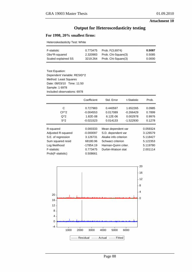
GRA 19003 Master Thesis 01.09.2010
Page 88
Attachment 10
Output for Heteroscedasticity testing
For 1998, 20% smallest firms:
Heteroskedasticity Test: White
F-statistic 0.773475 Prob. F(3,6974) 0.5087
Obs*R-squared 2.320983 Prob. Chi-Square(3) 0.5085
Scaled explained SS 3219.264 Prob. Chi-Square(3) 0.0000
Test Equation:
Dependent Variable: RESID^2
Method: Least Squares
Date: 08/03/10 Time: 11:50
Sample: 1 6978
Included observations: 6978 Coefficient Std. Error t-Statistic Prob.
C 0.727983 0.440597 1.652265 0.0985
CF^2 -0.004553 0.017089 -0.266429 0.7899
Q^2 1.82E-08 6.12E-06 0.002978 0.9976
S^2 -0.021523 0.014133 -1.522930 0.1278
R-squared 0.000333 Mean dependent var 0.059324
Adjusted R-squared -0.000097 S.D. dependent var 3.126579
S.E. of regression 3.126731 Akaike info criterion 5.118427
Sum squared resid 68180.96 Schwarz criterion 5.122353
Log likelihood -17854.19 Hannan-Quinn criter. 5.119780
F-statistic 0.773475 Durbin-Watson stat 2.001114
Prob(F-statistic) 0.508661
-4
0
4
8
12
16
20
0
4
8
12
16
20
1000 2000 3000 4000 5000 6000
Residual Actual Fitted

GRA 19003 Master Thesis 01.09.2010
Page 89
1998 20 % largest
Heteroskedasticity Test: White
F-statistic 45.42115 Prob. F(3,6974) 0.0000
Obs*R-squared 133.7287 Prob. Chi-Square(3) 0.0000
Scaled explained SS 994.2248 Prob. Chi-Square(3) 0.0000
Test Equation:
Dependent Variable: RESID^2
Method: Least Squares
Date: 08/03/10 Time: 12:01
Sample: 1 6979
Included observations: 6978 Coefficient Std. Error t-Statistic Prob.
C 0.002973 0.004159 0.714851 0.4747
CF^2 0.012924 0.001121 11.52618 0.0000
Q^2 -2.05E-08 4.42E-08 -0.462395 0.6438
S^2 0.000150 7.78E-05 1.925744 0.0542
R-squared 0.019164 Mean dependent var 0.011555
Adjusted R-squared 0.018742 S.D. dependent var 0.044587
S.E. of regression 0.044167 Akaike info criterion -3.401117
Sum squared resid 13.60418 Schwarz criterion -3.397190
Log likelihood 11870.50 Hannan-Quinn criter. -3.399763
F-statistic 45.42115 Durbin-Watson stat 2.013634
Prob(F-statistic) 0.000000
-0.4
0.0
0.4
0.8
1.2
-0.4
0.0
0.4
0.8
1.2
1.6
1000 2000 3000 4000 5000 6000
Residual Actual Fitted

GRA 19003 Master Thesis 01.09.2010
Page 90
1999 20 % smallest
Heteroskedasticity Test: White
F-statistic 13.04764 Prob. F(3,8599) 0.0000
Obs*R-squared 38.98366 Prob. Chi-Square(3) 0.0000 Scaled explained SS 171.2535 Prob. Chi-Square(3) 0.0000
Test Equation: Dependent Variable: RESID^2 Method: Least Squares Date: 08/03/10 Time: 12:14 Sample: 1 8603 Included observations: 8603
Coefficient Std. Error t-Statistic Prob. C 0.065442 0.007365 8.885309 0.0000
CF^2 2.69E-06 4.96E-06 0.541200 0.5884 Q^2 2.04E-08 2.47E-07 0.082506 0.9342 S^2 -0.001459 0.000235 -6.213616 0.0000
R-squared 0.004531 Mean dependent var 0.019855
Adjusted R-squared 0.004184 S.D. dependent var 0.058882 S.E. of regression 0.058758 Akaike info criterion -2.830299 Sum squared resid 29.68851 Schwarz criterion -2.827017 Log likelihood 12178.53 Hannan-Quinn criter. -2.829180 F-statistic 13.04764 Durbin-Watson stat 1.969401 Prob(F-statistic) 0.000000
-0.4
0.0
0.4
0.8
1.2
1.6 0.0
0.4
0.8
1.2
1.6
2.0
1000 2000 3000 4000 5000 6000 7000 8000
Residual Actual Fitted

GRA 19003 Master Thesis 01.09.2010
Page 91
1999 20 % largest
Heteroskedasticity Test: White
F-statistic 2.533506 Prob. F(3,8600) 0.0551
Obs*R-squared 7.597338 Prob. Chi-Square(3) 0.0551
Scaled explained SS 48.32480 Prob. Chi-Square(3) 0.0000
Test Equation:
Dependent Variable: RESID^2
Method: Least Squares
Date: 08/03/10 Time: 12:20
Sample: 1 8604
Included observations: 8604 Coefficient Std. Error t-Statistic Prob.
C 0.016146 0.003121 5.173948 0.0000
CF^2 0.002276 0.001102 2.064114 0.0390
Q^2 -4.32E-09 1.47E-08 -0.294195 0.7686
S^2 -0.000100 5.65E-05 -1.774570 0.0760
R-squared 0.000883 Mean dependent var 0.010777
Adjusted R-squared 0.000534 S.D. dependent var 0.038460
S.E. of regression 0.038449 Akaike info criterion -3.678479
Sum squared resid 12.71391 Schwarz criterion -3.675197
Log likelihood 15828.82 Hannan-Quinn criter. -3.677359
F-statistic 2.533506 Durbin-Watson stat 2.014943
Prob(F-statistic) 0.055103
-0.2
0.0
0.2
0.4
0.6
0.8
1.00.0
0.2
0.4
0.6
0.8
1.0
1000 2000 3000 4000 5000 6000 7000 8000
Residual Actual Fitted

GRA 19003 Master Thesis 01.09.2010
Page 92
2000 20 % smallest
Heteroskedasticity Test: White
F-statistic 12.19987 Prob. F(3,7627) 0.0000
Obs*R-squared 36.44393 Prob. Chi-Square(3) 0.0000
Scaled explained SS 2753.914 Prob. Chi-Square(3) 0.0000
Test Equation:
Dependent Variable: RESID^2
Method: Least Squares
Date: 08/03/10 Time: 12:26
Sample: 1 7631
Included observations: 7631 Coefficient Std. Error t-Statistic Prob.
C 0.230295 0.038768 5.940384 0.0000
CF^2 0.000732 0.000317 2.308179 0.0210
Q^2 -5.03E-08 8.03E-07 -0.062709 0.9500
S^2 -0.006710 0.001251 -5.364486 0.0000
R-squared 0.004776 Mean dependent var 0.023528
Adjusted R-squared 0.004384 S.D. dependent var 0.289415
S.E. of regression 0.288780 Akaike info criterion 0.354218
Sum squared resid 636.0435 Schwarz criterion 0.357856
Log likelihood -1347.520 Hannan-Quinn criter. 0.355466
F-statistic 12.19987 Durbin-Watson stat 2.025330
Prob(F-statistic) 0.000000
-2
0
2
4
60
1
2
3
4
5
6
1000 2000 3000 4000 5000 6000 7000
Residual Actual Fitted

GRA 19003 Master Thesis 01.09.2010
Page 93
2000 20 % largest
Heteroskedasticity Test: White
F-statistic 11.53078 Prob. F(3,7629) 0.0000
Obs*R-squared 34.45426 Prob. Chi-Square(3) 0.0000
Scaled explained SS 199.8546 Prob. Chi-Square(3) 0.0000
Test Equation:
Dependent Variable: RESID^2
Method: Least Squares
Date: 08/03/10 Time: 12:32
Sample: 1 7633
Included observations: 7633 Coefficient Std. Error t-Statistic Prob.
C -0.002229 0.003878 -0.574924 0.5654
CF^2 0.003921 0.000834 4.704072 0.0000
Q^2 -5.35E-09 1.87E-08 -0.285857 0.7750
S^2 0.000256 7.49E-05 3.424230 0.0006
R-squared 0.004514 Mean dependent var 0.011224
Adjusted R-squared 0.004122 S.D. dependent var 0.038251
S.E. of regression 0.038172 Akaike info criterion -3.692912
Sum squared resid 11.11615 Schwarz criterion -3.689275
Log likelihood 14098.00 Hannan-Quinn criter. -3.691664
F-statistic 11.53078 Durbin-Watson stat 1.988336
Prob(F-statistic) 0.000000
-0.2
0.0
0.2
0.4
0.6
0.8
1.00.0
0.2
0.4
0.6
0.8
1.0
1000 2000 3000 4000 5000 6000 7000
Residual Actual Fitted

GRA 19003 Master Thesis 01.09.2010
Page 94
2001 20 % smallest
Heteroskedasticity Test: White
F-statistic 0.150562 Prob. F(3,7632) 0.9294
Obs*R-squared 0.451895 Prob. Chi-Square(3) 0.9293
Scaled explained SS 878.6389 Prob. Chi-Square(3) 0.0000
Test Equation:
Dependent Variable: RESID^2
Method: Least Squares
Date: 08/03/10 Time: 12:37
Sample: 1 7636
Included observations: 7636 Coefficient Std. Error t-Statistic Prob.
C 0.480422 0.609991 0.787589 0.4310
CF^2 -0.000124 0.002253 -0.055183 0.9560
Q^2 -1.29E-06 3.46E-05 -0.037278 0.9703
S^2 -0.013148 0.019602 -0.670715 0.5024
R-squared 0.000059 Mean dependent var 0.072714
Adjusted R-squared -0.000334 S.D. dependent var 4.537066
S.E. of regression 4.537823 Akaike info criterion 5.863295
Sum squared resid 157156.9 Schwarz criterion 5.866931
Log likelihood -22382.06 Hannan-Quinn criter. 5.864543
F-statistic 0.150562 Durbin-Watson stat 2.000515
Prob(F-statistic) 0.929367
-5
0
5
10
15
20
25
0
5
10
15
20
25
1000 2000 3000 4000 5000 6000 7000
Residual Actual Fitted

GRA 19003 Master Thesis 01.09.2010
Page 95
2001 20 % largest
Heteroskedasticity Test: White
F-statistic 15.13847 Prob. F(3,7633) 0.0000
Obs*R-squared 45.17045 Prob. Chi-Square(3) 0.0000
Scaled explained SS 237.5810 Prob. Chi-Square(3) 0.0000
Test Equation:
Dependent Variable: RESID^2
Method: Least Squares
Date: 08/03/10 Time: 12:42
Sample: 1 7638
Included observations: 7637 Coefficient Std. Error t-Statistic Prob.
C 0.014066 0.003720 3.780919 0.0002
CF^2 0.002937 0.000439 6.688589 0.0000
Q^2 -1.19E-09 8.57E-09 -0.138299 0.8900
S^2 -6.40E-05 7.34E-05 -0.870954 0.3838
R-squared 0.005915 Mean dependent var 0.011093
Adjusted R-squared 0.005524 S.D. dependent var 0.035999
S.E. of regression 0.035900 Akaike info criterion -3.815643
Sum squared resid 9.837412 Schwarz criterion -3.812008
Log likelihood 14574.03 Hannan-Quinn criter. -3.814396
F-statistic 15.13847 Durbin-Watson stat 1.973637
Prob(F-statistic) 0.000000
-0.2
0.0
0.2
0.4
0.6
0.8
1.00.0
0.2
0.4
0.6
0.8
1.0
1000 2000 3000 4000 5000 6000 7000
Residual Actual Fitted

GRA 19003 Master Thesis 01.09.2010
Page 96
2002 20 % smallest
Heteroskedasticity Test: White
F-statistic 3.579973 Prob. F(3,6729) 0.0133
Obs*R-squared 10.72918 Prob. Chi-Square(3) 0.0133
Scaled explained SS 2155.121 Prob. Chi-Square(3) 0.0000
Test Equation:
Dependent Variable: RESID^2
Method: Least Squares
Date: 08/03/10 Time: 12:48
Sample: 1 6733
Included observations: 6733 Coefficient Std. Error t-Statistic Prob.
C 0.270019 0.078639 3.433656 0.0006
CF^2 0.000493 0.000567 0.870021 0.3843
Q^2 -2.00E-07 4.68E-06 -0.042624 0.9660
S^2 -0.007845 0.002527 -3.104644 0.0019
R-squared 0.001594 Mean dependent var 0.027058
Adjusted R-squared 0.001148 S.D. dependent var 0.542683
S.E. of regression 0.542371 Akaike info criterion 1.614860
Sum squared resid 1979.444 Schwarz criterion 1.618909
Log likelihood -5432.427 Hannan-Quinn criter. 1.616258
F-statistic 3.579973 Durbin-Watson stat 2.003035
Prob(F-statistic) 0.013266
-2
0
2
4
6
80
2
4
6
8
1000 2000 3000 4000 5000 6000
Residual Actual Fitted

GRA 19003 Master Thesis 01.09.2010
Page 97
2002 20 % largest
Heteroskedasticity Test: White
F-statistic 4.798795 Prob. F(3,6730) 0.0024
Obs*R-squared 14.37419 Prob. Chi-Square(3) 0.0024
Scaled explained SS 69.68164 Prob. Chi-Square(3) 0.0000
Test Equation:
Dependent Variable: RESID^2
Method: Least Squares
Date: 08/03/10 Time: 12:52
Sample: 1 6734
Included observations: 6734 Coefficient Std. Error t-Statistic Prob.
C 0.010418 0.003474 2.998726 0.0027
CF^2 0.002935 0.000799 3.672526 0.0002
Q^2 3.13E-08 3.27E-08 0.956812 0.3387
S^2 -6.54E-06 6.77E-05 -0.096599 0.9230
R-squared 0.002135 Mean dependent var 0.010282
Adjusted R-squared 0.001690 S.D. dependent var 0.032038
S.E. of regression 0.032010 Akaike info criterion -4.044915
Sum squared resid 6.896023 Schwarz criterion -4.040867
Log likelihood 13623.23 Hannan-Quinn criter. -4.043517
F-statistic 4.798795 Durbin-Watson stat 2.020234
Prob(F-statistic) 0.002429
-0.2
0.0
0.2
0.4
0.6
0.8
1.0
-0.2
0.0
0.2
0.4
0.6
0.8
1.0
1000 2000 3000 4000 5000 6000
Residual Actual Fitted

GRA 19003 Master Thesis 01.09.2010
Page 98
2003 20 % smallest
Heteroskedasticity Test: White
F-statistic 18.91214 Prob. F(3,7732) 0.0000
Obs*R-squared 56.35226 Prob. Chi-Square(3) 0.0000
Scaled explained SS 13074.34 Prob. Chi-Square(3) 0.0000
Test Equation:
Dependent Variable: RESID^2
Method: Least Squares
Date: 08/03/10 Time: 12:58
Sample: 1 7736
Included observations: 7736 Coefficient Std. Error t-Statistic Prob.
C 0.364518 0.087447 4.168450 0.0000
CF^2 0.005587 0.000922 6.060575 0.0000
Q^2 -4.01E-07 5.00E-06 -0.080159 0.9361
S^2 -0.010835 0.002797 -3.874257 0.0001
R-squared 0.007284 Mean dependent var 0.029485
Adjusted R-squared 0.006899 S.D. dependent var 0.635510
S.E. of regression 0.633314 Akaike info criterion 1.924816
Sum squared resid 3101.202 Schwarz criterion 1.928412
Log likelihood -7441.190 Hannan-Quinn criter. 1.926049
F-statistic 18.91214 Durbin-Watson stat 2.009165
Prob(F-statistic) 0.000000
-2
0
2
4
6
8
-2
0
2
4
6
8
1000 2000 3000 4000 5000 6000 7000
Residual Actual Fitted

GRA 19003 Master Thesis 01.09.2010
Page 99
2003 20 % largest
Heteroskedasticity Test: White
F-statistic 10.35129 Prob. F(3,7732) 0.0000
Obs*R-squared 30.94566 Prob. Chi-Square(3) 0.0000
Scaled explained SS 158.4194 Prob. Chi-Square(3) 0.0000
Test Equation:
Dependent Variable: RESID^2
Method: Least Squares
Date: 08/03/10 Time: 13:03
Sample: 1 7737
Included observations: 7736 Coefficient Std. Error t-Statistic Prob.
C 0.015774 0.003484 4.527776 0.0000
CF^2 0.001118 0.000209 5.338528 0.0000
Q^2 -1.84E-09 1.98E-08 -0.093118 0.9258
S^2 -0.000104 6.75E-05 -1.541588 0.1232
R-squared 0.004000 Mean dependent var 0.010521
Adjusted R-squared 0.003614 S.D. dependent var 0.033685
S.E. of regression 0.033624 Akaike info criterion -3.946624
Sum squared resid 8.741699 Schwarz criterion -3.943029
Log likelihood 15269.54 Hannan-Quinn criter. -3.945392
F-statistic 10.35129 Durbin-Watson stat 2.024864
Prob(F-statistic) 0.000001
-0.2
0.0
0.2
0.4
0.6
0.8
1.0
0.0
0.2
0.4
0.6
0.8
1.0
1000 2000 3000 4000 5000 6000 7000
Residual Actual Fitted

GRA 19003 Master Thesis 01.09.2010
Page 100
2004 20 % smallest
Heteroskedasticity Test: White
F-statistic 12.91841 Prob. F(3,5971) 0.0000
Obs*R-squared 38.53110 Prob. Chi-Square(3) 0.0000
Scaled explained SS 585.7590 Prob. Chi-Square(3) 0.0000
Test Equation:
Dependent Variable: RESID^2
Method: Least Squares
Date: 08/03/10 Time: 13:08
Sample: 1 5976
Included observations: 5975 Coefficient Std. Error t-Statistic Prob.
C 0.150156 0.022156 6.777141 0.0000
CF^2 0.000603 0.000284 2.125458 0.0336
Q^2 -6.51E-08 7.12E-07 -0.091463 0.9271
S^2 -0.003907 0.000692 -5.645454 0.0000
R-squared 0.006449 Mean dependent var 0.025807
Adjusted R-squared 0.005950 S.D. dependent var 0.142410
S.E. of regression 0.141986 Akaike info criterion -1.065512
Sum squared resid 120.3749 Schwarz criterion -1.061030
Log likelihood 3187.217 Hannan-Quinn criter. -1.063955
F-statistic 12.91841 Durbin-Watson stat 1.997402
Prob(F-statistic) 0.000000
-1
0
1
2
3 0.0
0.5
1.0
1.5
2.0
2.5
3.0
1000 2000 3000 4000 5000
Residual Actual Fitted

GRA 19003 Master Thesis 01.09.2010
Page 101
2004 20 % largest
Heteroskedasticity Test: White
F-statistic 4.969625 Prob. F(3,5974) 0.0019
Obs*R-squared 14.88172 Prob. Chi-Square(3) 0.0019
Scaled explained SS 62.28888 Prob. Chi-Square(3) 0.0000
Test Equation:
Dependent Variable: RESID^2
Method: Least Squares
Date: 08/03/10 Time: 13:12
Sample: 1 5978
Included observations: 5978 Coefficient Std. Error t-Statistic Prob.
C 0.014440 0.004271 3.380670 0.0007
CF^2 0.005257 0.001385 3.795772 0.0001
Q^2 -9.60E-09 1.98E-08 -0.485711 0.6272
S^2 -3.56E-05 8.10E-05 -0.439064 0.6606
R-squared 0.002489 Mean dependent var 0.012800
Adjusted R-squared 0.001988 S.D. dependent var 0.037062
S.E. of regression 0.037025 Akaike info criterion -3.753775
Sum squared resid 8.189488 Schwarz criterion -3.749294
Log likelihood 11224.03 Hannan-Quinn criter. -3.752219
F-statistic 4.969625 Durbin-Watson stat 1.998569
Prob(F-statistic) 0.001912
-.2
.0
.2
.4
.6
.8
-0.2
0.0
0.2
0.4
0.6
0.8
1.0
1000 2000 3000 4000 5000
Residual Actual Fitted

GRA 19003 Master Thesis 01.09.2010
Page 102
Marthe Kristine Hafsahl Karset 0801282
Elise Botten 0785153
BI Norwegian School of Management
GRA 19002 - Preliminary Thesis Report
Financial Constraints
for
Norwegian Private Firms
Hand-in date:
15.01.2010
Campus:
BI Oslo
Programme:
Master of Science in Business and Economics
Supervisor:
Bogdan Stacescu

GRA 19003 Master Thesis 01.09.2010
Page 103
Table of Content
Summary………………………………………………………………..…ii
4. Introduction…………………………………………………………….…1
5. Literature Review………………………………………………………….2
2.1 Characteristics of private firms………………………………………..2
2.2 Financial Constraints………………………………………………….3
2.3 The determinants of Financial Constraints……………………………5
2.4 Financial Constraints and a firm’s dividend policy
and capital structure…………………………………………………...7
2.4.1 Dividend Policy……………………………………………..7
2.4.2 Capital Structure…………………………………………….8
3. Methodology………………………………………………………………..9
4. Data………………………………………………………………………..12
5. Research Question…………………………………………………………13
Reference List……………………………………………………………..14

GRA 19003 Master Thesis 01.09.2010
Page 104
Summary
This preliminary thesis report aims to be an introduction and starting point to our
mater thesis where we aspire to investigate Norwegian Private Firms (Non-listed
firms). The purpose of our paper is to find a measure for financial constraints and
examine if there are differences between private and public firms with regard to
this measure. Finally, we will explore the relationship between those constraints
and firm specific variables like dividend payment and capital structure.
In section 1, we give an introduction to the subject.
In section 2, we present an extensive review of previous research and findings
within our field of study in order to develop a knowledge base concerning our
research questions.
In section 3, contains a description and explanation of the methodology of using
Euler Equations in order to find a measure for financial constraints.
In section 4, we briefly explain how we will start the process of gathering and
analyzing our data.
In section 5, our research questions are presented. These propositions are to some
extent confirmed by findings in the literature we have reviewed in section 2. We
would like to investigate these propositions:
Proposition 1: Non-listed firms are more financially constrained than listed firms.
Proposition 2: Firms facing financial constrains pay out less dividends than
unconstrained firms.
Proposition 3: Firms facing financial constraints have more debt than
unconstrained firms.
In addition we may want to extend our work with more research questions as we
dig deeper into the subject.

GRA 19003 Master Thesis 01.09.2010
Page 105
1. Introduction
The purpose of this thesis is to examine non-listed firms. Our staring point is that
non-listed firms do not have access to capital markets, thus this firms cannot
easily issue new equity compared to listed firms. Based on this, one might expect
that non-listed firms are more financially constrained than listed firms are.
In this thesis we want to find a measure for financial constraints and examine the
existence of financial constraints for non-listed firms and listed firms. Then we
will compare these results and analyze whether or not the difference is statistically
significant.
In order to find a measure for financial constraints, we would to like to use the
Euler equation approach, based on the framework established in the article
Financial Constraints Risk by Whited and Wu (2003).
Additionally, we would like to study the relationship between financial constraints
a firm’s dividend payout policy, capital structure and possible other firm specific
variables.

GRA 19003 Master Thesis 01.09.2010
Page 106
2. Literature Review
2.1 Characteristics of private firms
Private firms amount to a huge part of the overall economy. About 80-90 % of all
Norwegian firms are private firms. (Berzins and Bøhren 2008). The research on
private firms, in terms of finance and governance, are fairly modest. One
explanation could be the limited access to data on private firms and the fact that
they do not have a market price.
Non- listed firms differ from public firms in many ways, thus there is need for
separate research. Compared to listed firms, private firms have no market price,
not for the firm nor for the equity of the firm. Private firms operate in a less open
equity market, thus it can be harder for them to achieve equity finance. However,
this can make the danger of takeovers lower for private firms.
Recent research by Berzins and Bøhren (2008) also states that private and public
firms vary in terms of regulation. Minority owners in private firms can
experience to be less protected in private firms due to less regulation.
Moreover, private firms are less transparent than public firms, especially in terms
of information.
Finally, the stock- liquidity of private firms is to a greater extent lower than of
public firms. This can lead to less short term earnings pressure.
Transformation of research done on public firms cannot easily be transformed to
count for private firms as well. These differences make it interesting to do
research on financial constraints on both sectors and comparing them, to study to
what extent these differences are related with financial constraints.
Research done by Berzins and Bøhren (2008) discovered that private firms,
compared to public firms, have more debt and shorter debt and higher dividends
pr unit of earnings. Moreover, private firms are small and often much smaller than
public.
However, large firms tend to be private. 900 of Norway’s 1000 larges firms are in
fact private.

GRA 19003 Master Thesis 01.09.2010
Page 107
With regard to these findings our intuition that non-listed firms are more
financially constrained seems to be reasonable.
2.2 Financial Constraints
There are several definitions of Financial Constraints. Kaplan and Zingales (1995)
give this definition: “A firm is financially constrained if the cost of availability of
external funds precludes the company from making an investment it would have
chosen to make had internal funds been available”.
Almeira et al. (2003) also gives a definition of financial constraints which is
interesting for the purpose of this thesis. Inspired by Keynes(1936;196), they
writes that if a firm has unrestricted access to external capital, the firm is
financially unconstrained and there is no need to safeguard against future
investment needs and corporate liquidity becomes irrelevant.
With regard to the intuition that private firms not have unrestricted access to
external capital, the hypothesis that private firms may be more financially
constrained than public firms, seems reasonable.
Several studies have revealed that the significance of financial constraints is most
likely to fluctuate over the business cycle and with the position of monetary
policy. Structural changes in financial markets can change the degree of the
importance of the composition of internal and external finance. These changes
may influence the impact of financial constraints over time (Schiantarelli 1995).
One of the first to do a study within the area of financial constraints was Fazzari et
al. (1988). They pointed out the fact that in perfect capital markets, a firm’s
investment decisions are independent of its financial condition. However, firms
are mostly not facing perfect capital markets and external funds are not always a
perfect substitute for internal capital, particularly in the short run. In this paper,
Fazzari et al. analyzed differences in investment in firms classified according to
their earnings retention practices. Their results show that financial factors affect
investments, and that the link between financing constraints and investment varies
by type of firm.

GRA 19003 Master Thesis 01.09.2010
Page 108
Almeida et al. (2003) used the link between financial constraints and a firm’s
demand for liquidity to develop a new test of the effect of financial constraints on
firm policies. Theirs starting point is that firms who are financially constrained
needs to save more of their incoming cash flows in order to be able to take on
positive NPV projects as they appear. The effect of financial constraints can
therefore be captured by a firm’s propensity to save cash out of incremental cash
flows. They have called this effect the cash flow sensitivity of cash.
While constrained firms should have a positive cash flow sensitivity of cash,
unconstrained firms’ cash savings should not be systematically related to cash
flow. Their main finding confirms this hypothesis; firms that are more likely to be
financially constrained, display a significantly positive cash flow sensitivity of
cash, while unconstrained firms do not.
These findings imply that financial constraints are an important determinant of
firm’s behavior. To be able to take on positive NPV projects in the future, firms
anticipating financial constraints in the future respond to those potential
constraints by hoarding cash today.
As originally proposed by Keynes (1936), a major advantage of a liquid balance
sheet is that it allows firms to undertake valuable projects when they arise
(Almeida et al. 2003;1).
The article giving the main framework for our thesis is Financial Constraints
Risk, written by Toni M. Whited and and Guojun Wu (2003). Inspired by among
others Fazzari et al. (1988), their starting point is that firms facing finance
constraints will have investments who strongly respond to movements in cash
flow (holding investment opportunities constant).
Tobin’s q has usually been used as a proxy for investment opportunities. Tobin’s
q is a Q ratio defined as a ratio between two valuations of the same physical asset;
market value over replacement value.
However, there are several difficulties in measuring q and using this as a proxy for
financial constraints.

GRA 19003 Master Thesis 01.09.2010
Page 109
In the paper “Financial constraints and investment”, Fabio Schiantarelli
investigates the methodological issues involved in testing for financial constraints
on the basis of Q models of investments. He finds that the essential problem in
using Q models in this matter is that average Q may be a very inaccurate
alternative for the shadow value of an additional unit of new capital. He suggests
addressing this problem by estimating the Euler equation for the capital stock
derived from the underlying model. The benefit of the Euler equation approach is
that it avoids relying on measures of profitability based on firm’s market value.
The Euler equation approach addresses the same maximization problem as Q
equations, but it reorganizes the first order condition in a different way.
Like in the paper by Whited and Wu, we will use Euler Equations in order to
avoid the difficulties of measuring q. Using Tobin’s q is not feasible for analyzing
non-listed firms. Since our thesis will include an examination of non-listed firms,
using Euler Equations is an interesting alternative approach.
2.3 The determinants of financial constraints
Based on earlier mentioned definitions, one might say that financial constraints
are highly related to the differences between the cost of internal- and external
finance.
In order to understand relevance of financial constraint, one has to understand
theories concerning capital structure. Capital structure can be defined as “a mix of
a company's long-term debt, specific short-term debt, common equity and
preferred equity. The capital structure is how a firm finances its overall operations
and growth by using different sources of funds” (Investopedia.com). Choosing an
optimal capital structure may help to reallocate risk more efficiently. In addition it
contributes to maintain liquidity in case of investment opportunities (Mjøs 2008).
The modern theory of capital structure has it’s origin in the Modigliani- Miller
paper. According to the Modigliani Miller irrelevance substitutes Theorem (1958),
a company’s capital structure should be unrelated to its value; it is irrelevant.
Internal and external finances is therefore claimed to be perfect, and the
company’s financing and investment decisions should not be affected by the

GRA 19003 Master Thesis 01.09.2010
Page 110
firms’ capital structure. However, with the existence of informational
asymmetries and contract enforcement problems, the irrelevance hypothesis fails
to perform, resulting in that the cost of external and internal finance are not
perfect substitutes. With the presence of this situation, one might say that financial
constraints exists (Schiantarelli 1995).
To recognize why internal and external financing sources may not be perfect
substitutes, one might look at different factors that affect capital structure. Many
theories states that that agency costs (costs due to conflicts of interests) determine
the capital structure of companies (Harris and Raviv 1991). One might say that
there are two main types of possible conflicts that can arise; between managers
and equity holders, and between debt holders and equity holders.
Other theories use asymmetric information as explanation of capital structure.
(Harris and Raviv 1991). Managers of the firm are assumed to have information
that the firm’s return and investment opportunities that outsiders do not possess.
This can for example lead to managerial discretion, where the manager exploits
the asymmetric information balance in a negative way for the firm, thereby
creating costs disadvantages of external finance/for the company (Stulz 1990).
The Pecking- order- theory can also help explain why different finance sources
not are perfect substitutes. This theory categorizes the several forms of finance
into a hierarchy. The theory states that due to the information asymmetry,
companies will choose this order of financing; First use retained earnings and
fund of current owners, then risk- free and risky debt and last raising new equity
(Mjøs 2008).
Private and public firms have as mentioned in part 2.1, different capital structures.
These differences are highly relevant for the explanation of why financial
constraint may appear and not. The theories above help enlighten the reasons why
they have different cap structure.

GRA 19003 Master Thesis 01.09.2010
Page 111
2.4 Financial Constraints and a firm’s Dividend Policy and Capital Structure
2.4.1 Dividend Policy
Paying dividend can serve many purposes, both negative and positive. This action
can signal that the firm does not have any positive NPV projects to invest in or it
can be used to signal their true worth to the market. It can signal good news
because it decreases the amount of free cash flow in the firm, thus reducing
agency costs. There exists three groups that are likely to be affected most by a
firm’s dividend policy; shareholders, management and bondholders. Therefore,
this action can lead to interest conflicts between the groups, at the worst leading to
agency costs for the firm.
Dividend- payout is an important factor to take in consideration. Allen and
Michaely (2002) found that payout policies are in fact not driven by the desire to
signal the value of the firm, rather they found evidence of that payout policy was
influenced of wanting to avoid potential overinvestment by managers. A challenge
is to develop a payout- policy that maximizes firm value, and at the same time
maximize the utility of the investors. (Allen and Michaely 2002)
Mjøs (2008) characterize dividend- payment to be “a strong indicator of “financial
health”. Furthermore, he describes that dividend- payers tend to not be financially
constrained and that these groups use a less amount of debt. He also states that
these firms have total returns, that is twice of those firms not paying dividend
Almeira et al. (2003; 14) groups constrained firms as firms who have significantly
lower payout rations than unconstrained firms. This is the same intuition as
proposed by Fazzari et al. (1988).
However, Berzins and Bøhren (2008) found that private firms tend to have higher
dividends per unit of earnings compared to public firms. This finding contradicts
our intuition.

GRA 19003 Master Thesis 01.09.2010
Page 112
2.4.2 Capital Structure
In this thesis, we will sort the firms into constrained and unconstrained firms by
suggesting that non-listed firms cannot easily issue new equity and are therefore
more financially constrained than listed firms. This assumption is supported by
previous studies like e.g. Kaplan and Zingales (1997) who demonstrates that
financially constrained firms have high debt to capital ratio, which is one of the
characteristics of non-listed firms (see section 2.1).
Theories examined by Schiantarelli (1995) suggest that “internal funds are less
costly than external finance” (Which also is supported by the Pecking- order
theory) . In addition it is important to highlight that outside finance can lead to
losses or increased risk (Mjøs 2008). Schiantarelli thereafter states that an increase
in liquidity is likely to lead to greater investment. These statements together
indicates that a private firm, which tend to be more dependent on the external
finance debt (which is more expensive), can experience lower liquidity and
therefore loose opportunities to invest in positive NPV project. One of the reasons
for this is that funds are needed to pay interest bearing debt, instead of being used
to invest in new projects.
This may support our intuition that Financial Constrained firms have a capital
structure with more debt.
We will develop a framework for analyzing the relationship between these firm
specific variables and financial constraints in the further steps of our thesis work.

GRA 19003 Master Thesis 01.09.2010
Page 113
3. Methodology
To find a measure for financial constraints, we will use an Euler Equation based
on the framework developed by Whited and Wu (2003; 5-8), based on the work
by Whited (1992, 1998).
The starting point is a partial-equilibrium investment model, where the firm
maximizes the expected present discounted value of future dividends:
is the value of firm i at time zero, is the expectation operator conditional
on firms i’s time zero information set, is the one period discount factor
common to all firms and is the form’s dividend.
The firm maximizes with respect to dividends (a) and capital stock
accumulation (b):
a:
b:
In a, we can see that the dividend is expressed by a profit function, ; the
real cost of capital, ; and investments, during time t. is the
beginning-of-period capital stock, is a shock to the profit function observed by
the firm at time t.
In b, the capital stock in one period is expressed by the investments plus the
discounted capital stock which depreciates because of expected inflation.
The Euler condition for is:
The right hand side of this equation represents the marginal adjustment and
purchasing cost of investing today. The left hand side represents the expected
discounted cost of waiting to invest until tomorrow. is the Lagrange multiplier
associated with a constraint on outside finance:

GRA 19003 Master Thesis 01.09.2010
Page 114
If the outside equity is binding, the effects of external finance constraints will
show up in the term
which is the relative shadow cost of external
financing. For a financially constrained firm, . For an unconstrained firm,
the term till be zero. In other words, this means that a constrained firm will act
like it has a higher discount rate and will avoid investing today and prefer
investing in the next period instead.
To make the model possible to estimate, the is replaced by an expectation
error term where ( = 0 and ( ) =
.
The main equation will then look like this:
Constant return to scale implies that =
, where is output
and is variable costs.
The adjustment cost function is parameterized like this:
=
Where , m=2,…, M are coefficients to be estimated and M is a truncation
parameter that sets the highest power of / .
By substituting =
into the main equation and differentiating
the parameterized adjustment cost function with respect to and and
substituting the derivatives into the main equation, gives us the final estimating
equation:

GRA 19003 Master Thesis 01.09.2010
Page 115
in this model is unobservable, but possible to estimate by using observable
firm characteristics. In fact, this parameter will be the main interesting parameter
for us, as this will be the index of financial constraints. The lower the value of ,
the greater the financial constraint for the firms is.
can be estimated both for listed and non-listed firms. Whited and Wu (2003)
specifies like this:
Where is the ratio of the long term debt to total assets, is an
indicator that takes the value of one of the firm pays cash dividends, is a
firms sales growth, is the natural log of total assets, is the firm’s
three-digit industry sales growth, is the ratio of liquid assets to total
assets, is the ratio of cash flow to total assets, is the number of analysts
following the firm and is the three-digit industry debt to assets ratio.
One of the advantages of this model is that it takes variables like sales growth and
industry sales growth, which is a good thing since our intuition is that only firms
with good investment opportunities are likely to want to invest enough to be
constrained. These firms are expected to belong to industries which have a high
industry growth, but low industrial sales growth.
One of the purposes of our study is to examine the existence of financial
constraints for non-listed firms and comparing this with the results for listed
firms. Using a framework inspired by the one presented above, will makes us able
to get a measure for financial constraints for both listed and non-listed firms.

GRA 19003 Master Thesis 01.09.2010
Page 116
However, we will have to make adjustments to this framework. This will be one
of the next steps in our thesis work.
4. Data
We will provide our data of Norwegian non-listed firms from the CCGR (Centre
for Corporate Governance Research) database. The statements extracted will be
annual. We want to use data samples from as many years as possible.
With regard to Norwegian listed firm- data, we will most likely use Datastream
and other databases to collect data.
Concerning criteria for selecting our observations, this will be one our next steps
in our thesis work.
In process of editing our data set, we will firstly eliminate firms that do not have
our required variables.
Our procedure will consist of the Euler equation as the starting point; see section 3
for detailed steps.
Thereafter we will use the program SAS in order to get our sample and data
management. Further we will use the estimation program Eviews to do
econometric analysis on our data material and models.

GRA 19003 Master Thesis 01.09.2010
Page 117
5. Research Question
With regard to our work so far, we have defined these research questions which
our thesis work will concentrated about:
Proposition 1: Non-listed firms are more financially constrained than listed firms.
Proposition 2: Firms facing financial constrains pay out less dividends than
unconstrained firms.
Proposition 3: Firms facing financial constraints have more debt than
unconstrained firms.
In addition we may want to extend our work with more research questions as we
dig deeper into the subject.

GRA 19003 Master Thesis 01.09.2010
Page 118
Reference List
Almeida, Heitor, Murillo Campello and Michael S. Weisbach. 2003. The Cash
Flow Sensitivity of Cash.
Berzins, Janis, Øyvind Bøhren and Pål Rydland. 2008. Corporate finance and
governance in firms with limited liability: basic characteristics. Research Report.
Fazzari, Steven M., R. Glenn Hubbard, Bruce C. Petsersen. 1988. Financing
Constraints and Corporate Investment. Brookings Papers on Economic Activity.
No.1, 1988, 14 1-206.
Franklin, Allen and Roni Michaely. 2002. Payout Policy. North-Holland
Handbook of Economics.
Harris, Milton and Artur Raviv. 1991. The Theory of Capital Structure. The
Journal of Finance, Vol. 46. No.1 (Mar., 1991), pp.297-355.
Kaplan S. and L. Zingales, 1997. Do Financing Constraints Explain Why
Investment is Correlated with Cash Flow? Quarterly Journal of Economics, 112:
169-216.
Kaplan, S. N. and L. Zingales. 1995. Do Financing Constraints Explain Why
Investment is Correlated with Cash Flow? Working Paper no.5267, National
Bureau of Economic Research.
Keynes, J. M. 1936. The General Theory of Employment, Interest and Money.
London: McMillan.
Mjøs, Aksel. 2008. Norwegian Companies’ Capital Structure – An Overview.
Modligliani F. and M. H. Miller. 1958. The Cost of Capital, Corporation Finance
and the Theory of Investment. American Economic Review. 48: 261-97.

GRA 19003 Master Thesis 01.09.2010
Page 119
Sciantarelli, Fabio. 1995. Financial Constraints and Investment: A critical Review
of Methodological Issues and International Evidence. Conference Paper.
Stulz, Rene M C. 1990. Managerial Discretion and Optimal Financing Policies.
Whited, Toni M. 1992. Debt, Liquidity, Constraints and Corporate Investment.
The Journal of Finance, Vol.47, No.4. (Sept.,1992), pp 1425-1460
Whited, Toni M. and Guojun Wu. 2003. Financial Constraints Risk.
Web-pages:
www.investopedia.com