Embed Size (px)
Citation preview
FI-A2-engb 1/2016 (1003)
Finance Kenneth J Boudreaux

This course text is part of the learning content for this Edinburgh Business School course.
In addition to this printed course text, you should also have access to the course website in this subject, which will provide you with more learning content, the Profiler software and past examination questions and answers.
The content of this course text is updated from time to time, and all changes are reflected in the version of the text that appears on the accompanying website at http://coursewebsites.ebsglobal.net/.
Most updates are minor, and examination questions will avoid any new or significantly altered material for two years following publication of the relevant material on the website.
You can check the version of the course text via the version release number to be found on the front page of the text, and compare this to the version number of the latest PDF version of the text on the website.
If you are studying this course as part of a tutored programme, you should contact your Centre for further information on any changes.
Full terms and conditions that apply to students on any of the Edinburgh Business School courses are available on the website www.ebsglobal.net, and should have been notified to you either by Edinburgh Business School or by the centre or regional partner through whom you purchased your course. If this is not the case, please contact Edinburgh Business School at the address below:
Edinburgh Business School Heriot-Watt University Edinburgh EH14 4AS United Kingdom
Tel + 44 (0) 131 451 3090 Fax + 44 (0) 131 451 3002 Email [email protected] Website www.ebsglobal.net
The courses are updated on a regular basis to take account of errors, omissions and recent developments. If you'd like to suggest a change to this course, please contact us: [email protected].
Finance
Kenneth J Boudreaux is Professor of Economics and Finance at the AB Freeman School of Business, Tulane University, New Orleans, US.
Professor Boudreaux is an eminent scholar in finance, known widely for his ability to combine cutting-edge knowledge of the field with understandable explanations to professionals. In addition to being a successful researcher and university professor, he has for the past two decades lectured extensively to executives on topics in finance, in all parts of the world. Professor Boudreaux is the co-author of The Basic Theory of Corporate Finance, a widely used graduate-level text, and has published significant scholarly research on issues in corporate finance, securities markets and corporate restructuring. His research is frequently cited in journals of finance and economics world wide.
Professor Boudreaux is an active consultant to the business world, and regularly performs analyses involving financial issues for firms across industries that include shipping, petroleum exploration and production, airlines, consumer products and computers. Included on this list are: Atlantic Container Lines, British Petroleum, Central Gulf Lines, Exxon, Hewlett-Packard, Petroleum Helicopters and Reckitt & Colman.
Notwithstanding Professor Boudreaux’s wide experience, all organisations referred to in the worked examples are for illustrative purposes only and are entirely fictitious.

First Published in Great Britain in 1996.
© Kenneth J Boudreaux 2002, 2003
The rights of Kenneth J Boudreaux to be identified as Author of this Work has been asserted in accord-ance with the Copyright, Designs and Patents Act 1988.
All rights reserved; no part of this publication may be reproduced, stored in a retrieval system, or transmitted in any form or by any means, electronic, mechanical, photocopying, recording, or otherwise without the prior written permission of the Publishers. This book may not be lent, resold, hired out or otherwise disposed of by way of trade in any form of binding or cover other than that in which it is published, without the prior consent of the Publishers.
Finance Edinburgh Business School v
Contents
Module 1 The Basic Ideas, Scope and Tools of Finance 1/1 1.1 Introduction 1/1 1.2 Financial Markets and Participants 1/3 1.3 A Simple Financial Market 1/6 1.4 More Realistic Financial Markets 1/18 1.5 Interest Rates, Interest Rate Futures and Yields 1/30 Learning Summary 1/42 Review Questions 1/43 Case Study 1.1: Bond and Interest Rate Arithmetic 1/48 Case Study 1.2: A Multiple-Period Resource Reallocation 1/49
Module 2 Fundamentals of Company Investment Decisions 2/1 2.1 Introduction 2/1 2.2 Investment Decisions and Shareholder Wealth 2/2 2.3 Investment Decisions in All-Equity Corporations 2/6 2.4 Investment Decisions in Borrowing Corporations 2/10 2.5 Share Values and Price/Earnings Ratios 2/13 Learning Summary 2/17 Review Questions 2/17
Module 3 Earnings, Profit and Cash Flow 3/1 3.1 Introduction 3/1 3.2 Corporate Cash Flows 3/2 3.3 Cash Flows and Profits 3/8 Learning Summary 3/12 Review Questions 3/13
Module 4 Company Investment Decisions Using the Weighted Average Cost of Capital 4/1 4.1 Introduction 4/1 4.2 Free Cash Flow and Profits for Borrowing Corporations 4/2 4.3 Investment Value for Borrowing Corporations 4/6 4.4 Investment NPV and the Weighted Average Cost of Capital 4/8 4.5 The Adjusted Present Value Technique 4/14 4.6 The Choice of NPV Techniques 4/16
Contents
vi Edinburgh Business School Finance
Learning Summary 4/18 Review Questions 4/21
Module 5 Estimating Cash Flows for Investment Projects 5/1 5.1 Introduction 5/1 5.2 A Cash-Flow Estimation Example 5/4 5.3 Calculating the NPV, APV and IRR of the Example 5/12 Learning Summary 5/14 Review Questions 5/18
Module 6 Applications of Company Investment Analysis 6/1 6.1 Introduction 6/2 6.2 The Payback Period 6/2 6.3 The Average (Accounting) Return on Investment 6/4 6.4 Internal Rate of Return vs. Net Present Value 6/5 6.5 The Cost–Benefit Ratio and the Profitability Index 6/15 6.6 Summary of Alternatives to the NPV 6/17 6.7 Capital Rationing 6/18 6.8 Investment Interrelatedness 6/22 6.9 Renewable Investments 6/25 6.10 Inflation and Company Investment Decisions 6/28 6.11 Leasing 6/34 6.12 Managing the Investment Process 6/38 Learning Summary 6/41 Review Questions 6/42
Module 7 Risk and Company Investment Decisions 7/1 7.1 Introduction 7/1 7.2 Risk and Individuals 7/3 7.3 The Market Model and Individual Asset Risk 7/10 7.4 Using the Capital Asset Pricing Model in Evaluating Company Investment
Decisions 7/17 7.5 Other Considerations in Risk and Company Investments 7/26 Learning Summary 7/29 Review Questions 7/33 Case Study 7.1: NOSE plc 7/36
Contents
Finance Edinburgh Business School vii
Module 8 Company Dividend Policy 8/1 8.1 Introduction 8/1 8.2 Dividend Irrelevancy I 8/2 8.3 Dividends and Market Frictions 8/6 8.4 Dividend Clienteles: Irrelevancy II 8/11 8.5 Other Considerations in Dividend Policy 8/13 Learning Summary 8/16 Review Questions 8/18
Module 9 Company Capital Structure 9/1 9.1 Introduction 9/1 9.2 Capital Structure, Risk and Capital Costs 9/2 9.3 Capital Structure Irrelevance I: M&M 9/11 9.4 Capital Structure Decisions and Taxes 9/18 9.5 Capital Structure and Agency Problems 9/26 9.6 Making the Company Borrowing Decision 9/34 Learning Summary 9/40 Review Questions 9/41 Case Study 9.1: R-D Star Productions plc 9/43
Module 10 Working Capital Management 10/1 10.1 Introduction 10/1 10.2 Risk, Return and Term 10/2 10.3 Management of Short-Term Assets and Financings 10/8 10.4 Cash Budgeting and Short-Term Financial Management 10/21 Learning Summary 10/23 10.5 Appendix to Module 10: Financial and Ratio Analysis 10/24 Review Questions 10/46
Module 11 International Financial Management 11/1 11.1 Introduction 11/1 11.2 The Foreign Exchange Markets 11/3 11.3 International Financial Management 11/10 Learning Summary 11/16 Review Questions 11/18
Contents
viii Edinburgh Business School Finance
Module 12 Options, Agency, Derivatives and Financial Engineering 12/1 12.1 Introduction 12/2 12.2 Options 12/2 12.3 Agency 12/32 12.4 Derivatives 12/36 12.5 Financial Engineering 12/41 Learning Summary 12/43 12.6 Appendix 1 to Module 12: an Alternative Derivation of Binomial Call Option
Value 12/44 12.7 Appendix 2 to Module 12: A Numerical Application of Agency Theory 12/47 Review Questions 12/53
Appendix 1 Statistical Tables A1/1
Appendix 2 Examination Formula Sheet A2/1
Appendix 3 Practice Final Examinations A3/1
Practice Final Examination 1 3/2 Practice Final Examination 2 3/14 Examination Answers 3/25
Appendix 4 Answers to Review Questions A4/1
Module 1 4/1 Module 2 4/17 Module 3 4/19 Module 4 4/20 Module 5 4/22 Module 6 4/26 Module 7 4/29 Module 8 4/33 Module 9 4/35 Module 10 4/44 Module 11 4/47 Module 12 4/49
Index I/1
Finance Edinburgh Business School 1/1
Module 1
The Basic Ideas, Scope and Tools of Finance
Contents 1.1 Introduction .............................................................................................1/1 1.2 Financial Markets and Participants .......................................................1/3 1.3 A Simple Financial Market .....................................................................1/6 1.4 More Realistic Financial Markets ....................................................... 1/18 1.5 Interest Rates, Interest Rate Futures and Yields ............................. 1/30 Learning Summary ......................................................................................... 1/42 Review Questions ........................................................................................... 1/43 Case Study 1.1: Bond and Interest Rate Arithmetic .................................. 1/48 Case Study 1.2: A Multiple-Period Resource Reallocation ........................ 1/49
Learning Objectives
This module introduces the student to Finance as a subject area. It describes the participants in financial markets, the decisions they must make, and the basic process-es that are common to all such financial decisions. The module discusses the roles of borrowers, lenders, equity, security issuers and purchasers, and the sources of value for each. Because finance is inherently a quantitative and economic subject, this introductory module devotes much effort to instructing the student in the essential quantitative techniques of financial valuation, including discounting, present valuation, determination of rates of return, and some important financial economics relating to interest rates and security valuation. The module introduces some specialised financial concepts such as ‘yield to maturity’ and the ‘term structure’ of interest rates. It includes the first of several perspectives on the important company decision tools ‘net present value’ and ‘internal rate of return’. The module finishes with an illustration of the usefulness of even these basic financial techniques in understanding a market that remains mysterious to many financial practitioners: forward and futures markets for interest rates. In this module the student will learn the essence of the financial environment, along with the basic quantitative tools of financial valuation that are used throughout the course.
1.1 Introduction In this first module of the finance course you will study the basic concepts and techniques of analysis in finance. We shall investigate ideas of market value, of investment decision-making, of interest rates, and of various kinds of financial
Module 1 / The Basic Ideas, Scope and Tools of Finance
1/2 Edinburgh Business School Finance
markets. It is always good to have some general appreciation of a subject before its details are studied, and this is particularly true of finance, which is a very large and complex field of study. This module will supply you with that essential understanding, providing you with information on a number of fundamental concepts that can be applied again and again to the solution of real financial problems.
Finance is the economics of allocating resources across time. This definition, of course, is not particularly informative, but an example of a financial transaction that is governed by it may help you to understand the definition. Thus, suppose a new audio device, the digital audio tape player, has just come onto the market. Being an audiophile, you must have one. Economic logic says that if you had the resources to purchase it you would, because your satisfaction would increase by exchanging cash for the digital device. But suppose that you had neither the cash nor other assets that could be readily sold for enough cash to purchase the player. Would you be able to buy it?
The answer is that you may or may not be able to, depending upon whether you can convince someone to lend you the money. Whether you can is a function both of the tangible assets you have and the expectation of developing more assets in the future from which your creditor can expect to be paid. Because you do not have the tangible financial resources now to buy what you want, by borrowing you can shift some of your future resources back to the present so as to enable you to buy what you desire. You are buying the player with resources that you do not yet have in hand but are expected to get sometime in the future. And from the perspec-tive of the lender, an exactly opposite transaction will take place: the lender gives up some present resources in exchange for those that you are expected to provide in the future as you pay off the loan. This shifting around, or reallocation of re-sources in time, is the essence of finance.
This example is useful because it can also help us to understand why finance is an important subject. Think how many transactions have this essence of shifting resources around in time. We must include not only the borrowing and lending of money by individuals, but by governments, corporations and other institutions. And the borrowing and lending of money are not the only ways in which resources are reallocated in time. When a company issues equity capital (in other words, raises money from its owners) it is undertaking a financial transaction similar to your borrowing to get the tape player; that is, it is accepting money now and giving in exchange a promise to return money in the future (in the form of corporate dividends). The owners of the company are engaging in a financial transaction with the company that is very similar to the one that occurs between you and the lender in the financing of your tape player.
Think how many purchases and sales of tangible assets are made possible by the ability to shift resources across time. All personal credit purchases, much of corporate asset acquisition, and a great deal of a government’s providing of assets and services would not be possible without underlying financial transactions. Understanding the finance characteristic of these activities is an important part of being educated in business.
Module 1 / The Basic Ideas, Scope and Tools of Finance
Finance Edinburgh Business School 1/3
The above array of transactions that have important financial dimensions is im-pressive in its breadth, but it can be intimidating in the complexity it implies for the study of finance. We shall nowhere deny that finance is a large and complex field, but its study need not be terribly intricate, at least at the outset. In this course our approach will be first to create a very simple model of a financial market wherein participants (the individuals, companies and governments in the market) can engage in rudimentary financial transactions. That model is useful in acquainting ourselves with the basic ideas common to all financial transactions. Once these have been developed, we shall gradually include more and more realism in the model, until we can deal with the characteristics of financial markets and transactions that we see in actual practice.
1.2 Financial Markets and Participants In a developed economy most people participate frequently in financial markets. Individuals borrow from and lend to financial institutions such as banks. Corporations similarly transact with banks, but they also use financial markets through other intermediaries such as investment bankers (companies that help raise money directly from other companies and individuals), and insurance companies (which lend your insurance premiums to other companies). Governments also borrow and lend to individuals, companies and financial institutions.
It is useful to have a general picture in our minds of why companies, individuals and governments use financial markets. We already have one example: you can use the financial market to facilitate your purchase of the tape player. That transaction shifts some of your future resources to the present (by borrowing), and increases your satisfaction. Other types of participants often engage in the same type of transaction. Governments regularly shift future resources to the present so as to allow greater present consumption by citizens. They do that by borrowing in the financial markets with the promise to repay the loans with future cash inflows of the type expected by governments (taxes, more borrowing, etc.). One of the most common motivations for participating in financial markets is to shift future re-sources to the present so as to increase present consumption, and thus satisfaction.
On the other hand, individuals, governments and companies also sometimes find themselves with more current resources than they wish to consume at present. They can shift present resources to the future by making them available to the financial markets. They can shift these resources by lending them, by buying ordinary (ownership) shares in a company, or by a number of other transactions. In exchange for giving up current resources, they get an expectation of increased future re-sources in the form, for example, of interest and principal payments from the amounts lent, and dividends and capital gains on the ordinary shares purchased. Individuals and institutions engaging in such transactions are happier with less present and more future resources, and that is their motivation for participating in financial markets. The money that they provide to the financial markets, of course, is the same money borrowed by others wishing to increase their present consump-tion by shifting resources from the future to the present. Depending upon a participant’s resources and preferences for consuming them across time, that
Module 1 / The Basic Ideas, Scope and Tools of Finance
1/4 Edinburgh Business School Finance
participant may at various times be a lender, a borrower, or both. Such financial transactions are motivated by a desire to increase satisfaction by changing the time allocation of resources.
Financial market participants borrow or otherwise raise money not only to alter their patterns of consumption but also to make investments in real assets. In finance, we distinguish between financial investments (such as borrowing, lending or buying ordinary shares), and real asset investments (such as building a new factory or buying a piece of equipment to be used in production). Whereas financial investments serve the purpose of reallocating resources across time, real asset investment can actually create new future resources that did not before exist. Real asset investment is obviously an important activity. Many economists feel that it may be the single most important activity in determining how wealthy people are.
Without financial markets, however, participants with ideas for good investments would find it difficult or impossible to get the money necessary to undertake those investments. Financial markets are the bridge between those willing to give up present consumption of resources in order to increase future consumption, and those in need of present resources in order to undertake real asset investment. This is another important function of financial markets.
The provision of funds for real asset investment is important, but just as im-portant is the allocative information that financial markets provide to those interested in making real asset investments. Financial markets can help the investor tell whether a proposed real asset investment is worthwhile by comparing the returns from the investment with those available on competing uses of the re-sources. If the financial market did not do that, some other authority, such as the government, would. There often are significant differences between the decisions that would be made by a government and by competitive financial markets.
There is one other important service provided by financial markets to partici-pants. We can describe this generally as risk adjustment. We are not yet ready to give a rigorous definition of risk in financial transactions, but your own intuitions about risk will serve as an acceptable definition for now. Financial market partici-pants are risk-averse. That phrase means that their dislike for risk would, for example, cause them to choose the less risky of two otherwise identical investments. This implies not that participants reject risky transactions, but that the riskiness of an opportunity affects the price that they are willing to pay for it. Because financial markets have such wide variety of riskinesses available, participants can combine borrowings, lendings, the buying and selling of shares, and other transactions to shape the riskiness of their position to be whatever makes them most satisfied. Such decisions made by participants also influence the information that financial markets give to potential real asset investors, as above.
In sum, financial markets allow participants to reallocate resources across time, to decide correctly about – and make – real asset investments, and shape the riskiness of their holdings. All of these services are inherent in the transactions that partici-pants make in those markets.
Module 1 / The Basic Ideas, Scope and Tools of Finance
Finance Edinburgh Business School 1/5
1.2.1 Market Interest Rates and Prices
When some participants wish to bring future resources to the present by borrowing, and others wish to shift present resources to the future by lending, the possibility of beneficial transactions is obvious (the potential lenders can provide current re-sources to the potential borrowers in exchange for the borrowers’ promises to provide future resources to the lenders, making both groups happier). But they must decide on the amount of future resources to be exchanged for present ones. In other words, the lenders and borrowers must agree how many pounds of future resources it will be necessary to expect in exchange for each pound of current resources provided.
The financial market makes that decision for participants by setting the market interest rate. The market interest rate is the rate of exchange between present and future resources. It tells participants how many pounds are expected to be provided in the future for each pound of resources provided now. For example, if the market interest rate is 8 per cent per year, a lender can expect to receive 108 at the end of the year for each 100 lent at the beginning. The 108 comprises the 100 originally lent plus 8 as interest or compensation for lending. The relative demand and supply of resources to be borrowed and lent determines the market interest rate. (The market interest rate is always positive, because lenders have the alternative of simply keeping their money, and will therefore not agree to getting less in the future than they give up now.)
There is actually no such thing as the market interest rate. There are many market interest rates, all of which exist at the same time. The reason why there can simulta-neously be many market interest rates is that interest rates can cover different lengths of time in the future, and different riskinesses of transactions. For example, it is entirely possible that the interest rate for borrowing across a two-year period is different from that for borrowing across a one-year period, because of the relative demand and supply of lendable resources over those times. And the interest rate that applies to borrowings by a risky company will be higher than that paid by the government (which controls the presses that can print currency to pay off its loans), because lenders are risk-averse and require greater expected compensation in future resources from risky borrowers.
From that perspective, there are even more ‘interest rates’ than we tend to regard as such. Suppose, for example, that you were to purchase ordinary shares from a company with the expectation of getting future dividends in return. We do not describe that transaction as lending money to the company, nor is there a quoted interest rate, but in general economic terms the transaction is very similar to lending. You are giving up present pounds for the expectation of future pounds. Financial markets do not quote an interest rate for your purchase of ordinary shares, but they do quote a price for the shares. And when you receive dividends or cash from selling the shares, you will earn a rate of return that is similar to an interest rate. In other words the market price is telling you how much you must ‘lend’ to the company in order to get the expected future dividends and increases in value. This information is almost the same as quoting a market interest rate for the transaction, as we shall now see.
Module 1 / The Basic Ideas, Scope and Tools of Finance
1/6 Edinburgh Business School Finance
1.3 A Simple Financial Market
1.3.1 Shifting Resources in Time
Financial markets are complicated when there are many different kinds of partici-pants, when the transactions that they make are risky, and when those transactions cover several periods of time. Before we finish studying finance we shall deal with all of those things. First, however, we must develop the basic concepts inherent in all financial transactions. We shall do this with the simplest financial model that can accomplish that goal. The first financial market we shall examine therefore has the following characteristics: 1. We assume away all ‘frictions’ such as taxes, costs of transacting (brokerage fees)
and costs of finding information. 2. We assume away all risk. Whenever a transaction is agreed upon, all of its terms
will be kept by everyone. 3. Time is very simple in this market. There is only ‘now’ and ‘later’, with one
period of time between. All financial transactions take place ‘now’ and have their resolution (for example, pay their interest and principal) ‘later’. In this kind of financial market we need not distinguish between types of partici-
pants, because individuals, governments and companies would all have the same risk (none), pay the same taxes (none), and last the same time (one period). That is not to say that all participants are exactly the same, however. As a matter of fact they will be different enough to present a surprisingly realistic picture of a quite diverse market.
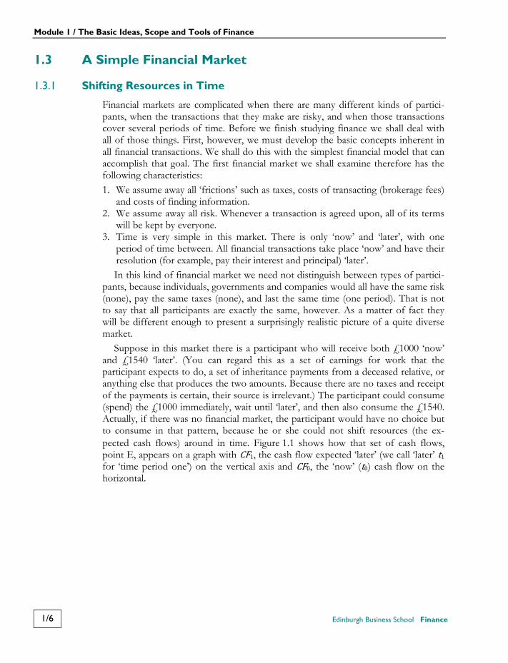
Suppose in this market there is a participant who will receive both £1000 ‘now’ and £1540 ‘later’. (You can regard this as a set of earnings for work that the participant expects to do, a set of inheritance payments from a deceased relative, or anything else that produces the two amounts. Because there are no taxes and receipt of the payments is certain, their source is irrelevant.) The participant could consume (spend) the £1000 immediately, wait until ‘later’, and then also consume the £1540. Actually, if there was no financial market, the participant would have no choice but to consume in that pattern, because he or she could not shift resources (the ex-pected cash flows) around in time. Figure 1.1 shows how that set of cash flows, point E, appears on a graph with CF1, the cash flow expected ‘later’ (we call ‘later’ t1 for ‘time period one’) on the vertical axis and CF0, the ‘now’ (t0) cash flow on the horizontal.
Module 1 / The Basic Ideas, Scope and Tools of Finance
Finance Edinburgh Business School 1/7
Figure 1.1 The financial exchange line
Suppose that the participant does not particularly like this pattern of consump-tion and prefers to consume somewhat more than £1000 at t0. He can accomplish that by borrowing some money at t0 with the promise to repay it with interest at t1. Suppose further that the balance of potential borrowers and lenders has resulted in a market interest rate of 10 per cent. With such a market interest rate, the participant could, for example, increase his t0 consumption to £1200 by borrowing £200 now and promising to repay that amount plus 10 per cent interest at t1. He would owe £200 × (1 + 10%), or £220 at t1, so at t1 he could consume £1540 minus £220, or £1320. The move from his original pattern (point E) to this new pattern (point A) is shown in Figure 1.1.
The financial market also allows participants to shift resources into the future by deferring current consumption. If the participant originally decides that £1000 of present consumption is too much, he could, for example, lend £300 of his t0 money and get in return an increase of £300 × (1.10) = £330 at t1. That transaction is shown as a move from E to B in Figure 1.1.
You may have noticed already that if we were to join all of the points we have discussed in Figure 1.1, they would form a straight line (we shall henceforth call this a financial exchange line, and for convenience we shall also use the letter i to stand for the interest rate). Actually, any transaction that a participant with this initial endowment might take by borrowing or lending at the market rate of interest will produce a result that lies on that straight line between the two axes. For
£7
00
£1
00
0
£1
20
0
£1870
£1540
£1320
F
B
E
A
P
£2
40
0
£2640
0 CF0
CF1
Module 1 / The Basic Ideas, Scope and Tools of Finance
1/8 Edinburgh Business School Finance
example, if all cash flows were transferred to t1, there would be £[1540 + (1000 × 1.10)], or £2640 for t1, and nothing for t0 (point F).1
On the other hand, if all cash flows were shifted to t0, the participant would have £1000 plus whatever he could borrow at t0 with a promise to repay £1540 at t1. How much is this? For each £1 we borrow at t0, we must repay £1 × (1 + i) at t1, so we can borrow (using CFt to mean ‘cash flow at time t’) where = (1 + )= (1 + ) Thus in our example: = £15401.10= £1400 The participant could borrow £1400 at t0 with the promise to pay £1540 at t1, the £1540 comprising £1400 of principal and £140 of interest. The maximum amount the participant could consume at t0 is thus £2400, consisting of the original £1000 cash flow, plus the £1400 which can be borrowed at t0 with the promise to repay £1540 at t1. This is point P in Figure 1.1, £2400 at t0 and £0 at t1.
Believe it or not we have just done a calculation and arrived at a result that is of the greatest importance and underlies many of the ideas of finance. Discovering that £1540 at t1 is worth £1400 at t0 is called finding the present value of the £1540. Present value is defined as the amount of money you must invest or lend at the present time so as to end up with a particular amount of money in the future. Here, you would necessarily invest £1400 at t0 at 10 per cent interest to end up with £1540 at t1, so £1400 is the present (t0) value of £1540 at t1. The person or institution that was willing to lend the participant £1400 must have done just that type of calculation.
Finding the present value of a future cash flow is often called discounting the cash flow. In the above example, £1400 is the ‘discounted value of the £1540’, or the ‘present value of the t1 £1540, discounted at 10 per cent per period’.
From the calculations above you can see the type of information that the present value gives us about the future cash flow it represents. For example, should the participant’s expectation of receiving t1 cash flow increase to greater than £1540, he could borrow more than £1400 at t0 (and vice versa for a smaller t1 expectation). Or if the t1 cash flow expectation becomes risky, the lender will require a return higher than 10 per cent to compensate for the risk being borne. (The risk here is that when t1 arrives, the full amount of the £1540 expectation does not appear.) If the interest rate
1 The market interest rate is thus really an ‘exchange rate’ between present and future resources. It tells us the price of t1 pounds in terms of t0 pounds. The exchange line in Figure 1.1 and the market interest rate are thus giving us the same basic information. It should not surprise you to hear that the steepness or slope of the exchange line (the ratio of exchanging t0 for t1 pounds) is determined by the market interest rate. The higher is the market interest rate, the more steep is the slope of the exchange line. In plain words, this says imply that the higher is the interest rate, the more pounds you must promise at t1 in order to borrow a pound at t0 – which you doubtless knew already!
Module 1 / The Basic Ideas, Scope and Tools of Finance
Finance Edinburgh Business School 1/9
increases, you can see that the present value, and thus the amount that the participant can borrow against it, declines. So the present value of a future cash flow is the amount that a willing and informed lender would agree to lend, getting in return a claim upon the future cash amount. The amount of the present value will depend upon the expected size and risk of the cash flow, and when it is expected to occur.
How much you can borrow by promising to pay an expected future amount is an important interpretation of present value, but by no means is it the only, or even the most important, interpretation. Present value is also an accurate representation of what the financial market does when it sets a price on a financial asset. For example, suppose that our participant does not wish to borrow money, but instead wishes to sell outright the expectation of receiving cash at t1. The participant can do this by issuing a security that endows its owner with the legal right to claim the t1 cash flow. This security could be a simple piece of paper with the agreement written upon it, or could be a very formal contract of the type issued by companies when they borrow money or issue shares.
For how much do you think the participant might sell such a security? Everyone thinking of buying will of course examine alternatives to buying this security. (Economists call such alternatives opportunity costs because they represent the ‘costs’ of doing this instead of something else, in the sense of an opportunity forgone.) They will discover that for each t0 £1 used to buy the security, £1.10 at t1 will be returned by other same-risk investments in the financial market (for example, lending at 10 per cent). That being the case, the participant will be able to sell the security for no more than £1400 (the present value of £1540 at t1 discounted at 10 per cent), because potential buyers need only lend £1400 to the financial market at t0 in order to get £1540 at t1, exactly what the security promises. And because of the competitive nature of financial markets, the security will not sell for less than £1400, because if it did it would provide a cash return the same as other alternatives, but at a lower present price. As potential buyers of the security begin bidding against each other, the security’s price must increase or decline to the point where its expected future cash flow costs the same as that future cash flow acquired by any other means.
Present value is thus the market value of a security when market interest rates or opportunity rates of return are used as discount rates. This is perhaps the most important application of the notion of present value.
This brings us to another important application of the present-value idea. We have seen that the present value of all of our participant’s present and future resources (cash flows) is £2400. This amount also has a special name in finance: it is known as present wealth. Present wealth is a useful concept in that it tells us the total value of a participant’s entire time-specified resources with a single number. It is even more important because it can be used as a benchmark or standard to judge whether someone is going to be better or worse off because of a proposed financial decision. But we shall need to introduce a few more ideas before we can develop that point as completely as it deserves.
One thing we can now see readily from Figure 1.1 is that one cannot change present wealth merely by transacting (borrowing and lending at the market rate) in
Module 1 / The Basic Ideas, Scope and Tools of Finance
1/10 Edinburgh Business School Finance
the financial market. Though borrowing and lending will move us up and down the financial exchange line, and thereby allow us to choose the time allocation of our present wealth that makes us most happy, such transactions cannot move the line and therefore cannot change our wealth. The reason is easy enough to deduce. In financial markets, by buying and selling securities (or borrowing and lending), the total amount of wealth that is associated with those securities is unchanged. So if one wishes to increase one’s wealth by buying and selling in those markets, one would be forced to find another participant who, doubtless inadvertently, would allow his wealth to be reduced. As we shall see soon, the odds of doing so are low.
1.3.2 Investing
If we cannot expect to change our wealth by transacting in financial markets, how can we get richer? The answer is by investing in real assets. This type of financial activity can change our present wealth because it is not necessary to find someone else to give us part of their wealth in order for ours to increase. Investing in real assets such as productive machinery, new production facilities, research, or a new product line to be marketed, because it creates new future cash flows that did not previously exist, can generate new wealth that was not there before.
Of course not all real-asset investments are wealth-increasing. Investments are not free; we must give up some resources in order to undertake an investment. If the present value of the amounts we give up is greater than the present value of what we gain from the investment, the investment will decrease our present wealth. Because that will allow us to consume less across time, it is a bad investment. Of course a good investment would produce more wealth than it uses, and would therefore be desirable.
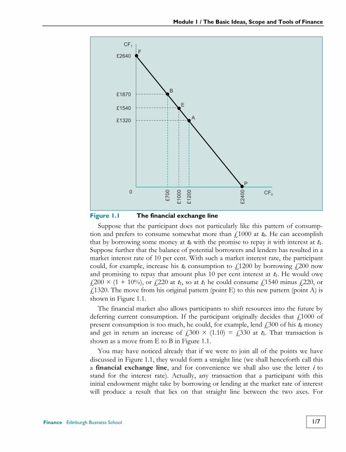
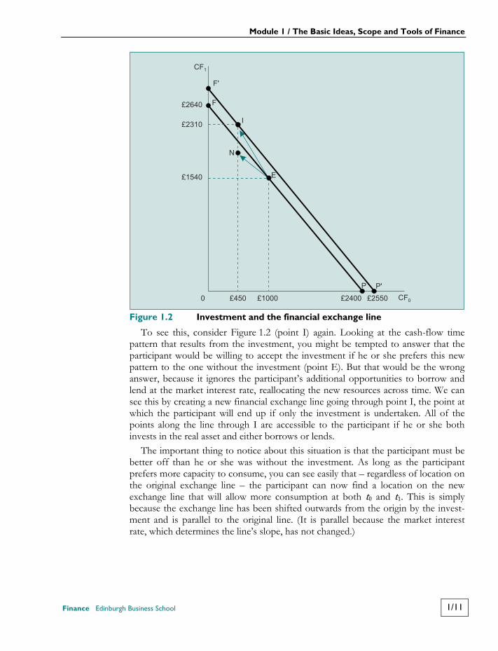
Figure 1.2 shows how real-asset investments work in our simple financial market. Suppose that our participant discovers an opportunity to invest £550 at t0 in a real asset that is expected to return £770 at t1. In Figure 1.2 this appears as a move from point E to point I. That investment would result in t1 resources of £2310 and t0 resources of £450. Should this opportunity be accepted or not? The answer is that it depends upon the effect on the participant’s present wealth.
Module 1 / The Basic Ideas, Scope and Tools of Finance
Finance Edinburgh Business School 1/11
Figure 1.2 Investment and the financial exchange line
To see this, consider Figure 1.2 (point I) again. Looking at the cash-flow time pattern that results from the investment, you might be tempted to answer that the participant would be willing to accept the investment if he or she prefers this new pattern to the one without the investment (point E). But that would be the wrong answer, because it ignores the participant’s additional opportunities to borrow and lend at the market interest rate, reallocating the new resources across time. We can see this by creating a new financial exchange line going through point I, the point at which the participant will end up if only the investment is undertaken. All of the points along the line through I are accessible to the participant if he or she both invests in the real asset and either borrows or lends.
The important thing to notice about this situation is that the participant must be better off than he or she was without the investment. As long as the participant prefers more capacity to consume, you can see easily that – regardless of location on the original exchange line – the participant can now find a location on the new exchange line that will allow more consumption at both t0 and t1. This is simply because the exchange line has been shifted outwards from the origin by the invest-ment and is parallel to the original line. (It is parallel because the market interest rate, which determines the line’s slope, has not changed.)
CF0
P'
F'
CF1
£2640
£2310
£1540
0 £450 £1000 £2400 £2550
N
E
I
F
P
Module 1 / The Basic Ideas, Scope and Tools of Finance
1/12 Edinburgh Business School Finance
We can calculate the amount of this parallel shift by seeing how far the line’s intercept has moved along the horizontal axis. As before, this means taking the present value of any position on the new line. Since we know point I already, we can use it: = (1 + )= £450 + £2310(1.10)= £2550
The outward shift in the exchange line is to £2550 at t0. But this is also the hori-zontal intercept of the new exchange line, which (from what we know about the discounted value of future resources) is our participant’s new present wealth. So we have also discovered that his or her present wealth will increase from its original level of £2400 to £2550 with the investment.
Remember that we are trying to connect the investment’s desirability to the par-ticipant’s change in present wealth. The last step in that process is easy: since any outward shift in the exchange line signals a good investment, and since any outward shift is an increase in present wealth, any investment that increases present wealth is a good one. That is simply another way of saying what we said earlier: investments are desirable when they produce more present value than they cost.
1.3.3 Net Present Value
Although you may have found it interesting to see how an investment is judged for desirability by calculating its effect on our participant’s present wealth, the technique is somewhat cumbersome. Fortunately, there is a much more direct method of testing the desirability of an investment, which gives the same answers as the present wealth calculation. This approach deals directly with the investment’s cash flows, and does not require that any particular participant’s resources be used in the calculation. In finance this technique is called net present value; it is simply the present value of the difference between an investment’s cash inflows and outflows.
Recall that our participant’s investment requires an outlay of £550 at t0, and returns £770 at t1. If we calculate the present value of the t1 cash inflow and subtract the (already present value of the) t0 outflow we get: PV inflow − PV outflow = (1 + ) −= £770(1.1) − £550= £700 − £550= £150
The difference between the present values of the cash inflows and outflows of
the investment is +£150. That number is the net present value of the investment. Net present value, or NPV as it is commonly known, is a very important concept
for a number of reasons. First, notice that the NPV of the investment, £150, is exactly equal to the change in the present wealth (£2550 − £2400) of our participant, were he
Module 1 / The Basic Ideas, Scope and Tools of Finance
Finance Edinburgh Business School 1/13
or she to undertake the investment. That is no accident. It is generally true that correctly calculated NPVs are always equal to the changes in present wealths of participants who undertake the investments. The NPV is thus an excellent substitute for our original laborious technique of calculating the change in present wealth of an investing participant. NPV gives us that number directly.
Why does NPV equal the increase in present wealth? We could use some algebra to show you, but a more important economic point can be made by considering the NPV as a reflection of how much the investment differs from its opportunity cost. Remember that our investor’s opportunity cost of undertaking the investment is the alternative of earning a 10 per cent return in the financial market. The investment costs £550 to undertake. If our participant had put that money in the financial market instead of the investment, he or she could have earned £550 × (1.1) = £605 at t1. Since the investment returned £770 at t1 the earnings were £770 – £605 = £165 more at t1 with the investment than with the next-best opportunity. The £165 is the excess return on the investment at t1. If we take the present value of that amount, = £165(1.1) = £150 we produce a number that we have seen before: the investment’s NPV. This gives us yet another important interpretation of NPV. It is the present value of the future amount by which the returns from the investment exceed the opportunity costs of the investor.
NPV is the most useful concept in finance. We shall encounter it in various im-portant financial decisions throughout the course, so it is most important that you appreciate its conceptual underpinnings, its method of calculation, and its varied applications. To review briefly what we have discovered about NPV: 1. The NPV of an investment is the present value of all of its present and future
cash flows, discounted at the opportunity cost of those cash flows. These oppor-tunity costs reflect the returns available on investing in an alternative of equal timing and equal risk.
2. The NPV of an investment is the change in the present wealth of the wise investor who chooses a positive NPV investment, and also of the unfortunate investor who chooses a negative NPV investment.
3. The NPV of an investment is the discounted value of the amounts by which the investment’s cash flows differ from those of its opportunity cost. When NPV is positive, the investment is expected to produce (in present value total) more cash across the future than the same amount of money invested in the comparable alternative.
1.3.4 Internal Rate of Return
Net present value is an excellent technique to use for investment decisions. But NPV is not the only investment decision technique that can allow us to make correct decisions. The internal rate of return (IRR) is another technique that can be used to make such decisions. It tells us how good or bad an investment is by calculating the average per-period rate of return on the money invested. Once
Module 1 / The Basic Ideas, Scope and Tools of Finance
1/14 Edinburgh Business School Finance
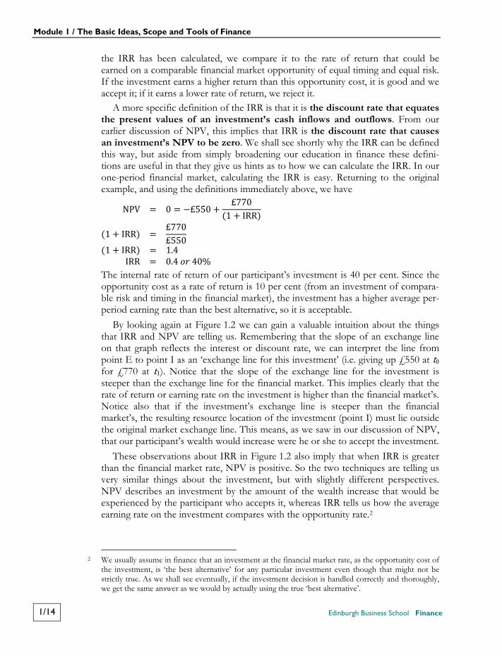
the IRR has been calculated, we compare it to the rate of return that could be earned on a comparable financial market opportunity of equal timing and equal risk. If the investment earns a higher return than this opportunity cost, it is good and we accept it; if it earns a lower rate of return, we reject it.
A more specific definition of the IRR is that it is the discount rate that equates the present values of an investment’s cash inflows and outflows. From our earlier discussion of NPV, this implies that IRR is the discount rate that causes an investment’s NPV to be zero. We shall see shortly why the IRR can be defined this way, but aside from simply broadening our education in finance these defini-tions are useful in that they give us hints as to how we can calculate the IRR. In our one-period financial market, calculating the IRR is easy. Returning to the original example, and using the definitions immediately above, we have NPV = 0 = −£550 + £770(1 + IRR)(1 + IRR) = £770£550(1 + IRR) = 1.4IRR = 0.4 40%
The internal rate of return of our participant’s investment is 40 per cent. Since the opportunity cost as a rate of return is 10 per cent (from an investment of compara-ble risk and timing in the financial market), the investment has a higher average per-period earning rate than the best alternative, so it is acceptable.
By looking again at Figure 1.2 we can gain a valuable intuition about the things that IRR and NPV are telling us. Remembering that the slope of an exchange line on that graph reflects the interest or discount rate, we can interpret the line from point E to point I as an ‘exchange line for this investment’ (i.e. giving up £550 at t0 for £770 at t1). Notice that the slope of the exchange line for the investment is steeper than the exchange line for the financial market. This implies clearly that the rate of return or earning rate on the investment is higher than the financial market’s. Notice also that if the investment’s exchange line is steeper than the financial market’s, the resulting resource location of the investment (point I) must lie outside the original market exchange line. This means, as we saw in our discussion of NPV, that our participant’s wealth would increase were he or she to accept the investment.
These observations about IRR in Figure 1.2 also imply that when IRR is greater than the financial market rate, NPV is positive. So the two techniques are telling us very similar things about the investment, but with slightly different perspectives. NPV describes an investment by the amount of the wealth increase that would be experienced by the participant who accepts it, whereas IRR tells us how the average earning rate on the investment compares with the opportunity rate.2
2 We usually assume in finance that an investment at the financial market rate, as the opportunity cost of
the investment, is ‘the best alternative’ for any particular investment even though that might not be strictly true. As we shall see eventually, if the investment decision is handled correctly and thoroughly, we get the same answer as we would by actually using the true ‘best alternative’.
Module 1 / The Basic Ideas, Scope and Tools of Finance
Finance Edinburgh Business School 1/15
The IRR and NPV techniques usually give the same answers to the question of whether or not an investment is acceptable. But they often give different answers to the question of which of two acceptable investments is the better. This is one of the major problems in finance, not so much because we do not know which one is correct but because many people seem to like the technique that gives the wrong answer! Obviously this deserves discussion, but we shall postpone that until we make the financial market a more realistic place, so the reasons for the disagree-ments between IRR and NPV can be explored more fully.
To review what we have discovered about the IRR technique: 1. IRR is the average per-period rate of return on the money invested in an
opportunity. 2. IRR is best calculated by finding the discount rate that would cause the NPV of
the investment to be zero. 3. To use IRR, we compare it with the return available on an equal-risk investment
of comparable cash-flow timing. If the IRR is greater than its opportunity cost, the investment is good, and we accept it; if it is not, we reject the investment.
4. IRR and NPV usually give us the same answer as to whether an investment is acceptable, but often different answers as to which of two investments is better. As a review of your understanding of some of the points we have made so far,
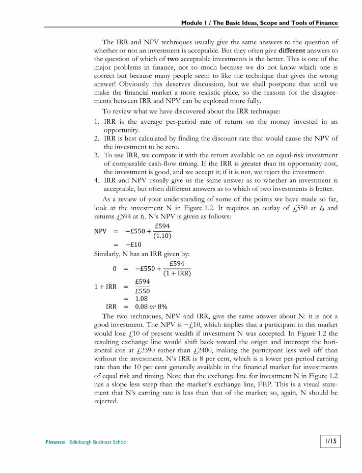
look at the investment N in Figure 1.2. It requires an outlay of £550 at t0 and returns £594 at t1. N’s NPV is given as follows: NPV = −£550 + £594(1.10)= −£10 Similarly, N has an IRR given by: 0 = −£550 + £594(1 + IRR)1 + IRR = £594£550= 1.08IRR = 0.08 8%
The two techniques, NPV and IRR, give the same answer about N: it is not a
good investment. The NPV is −£10, which implies that a participant in this market would lose £10 of present wealth if investment N was accepted. In Figure 1.2 the resulting exchange line would shift back toward the origin and intercept the hori-zontal axis at £2390 rather than £2400, making the participant less well off than without the investment. N’s IRR is 8 per cent, which is a lower per-period earning rate than the 10 per cent generally available in the financial market for investments of equal risk and timing. Note that the exchange line for investment N in Figure 1.2 has a slope less steep than the market’s exchange line, FEP. This is a visual state-ment that N’s earning rate is less than that of the market; so, again, N should be rejected.
Module 1 / The Basic Ideas, Scope and Tools of Finance
1/16 Edinburgh Business School Finance
1.3.5 A Simple Corporate Example
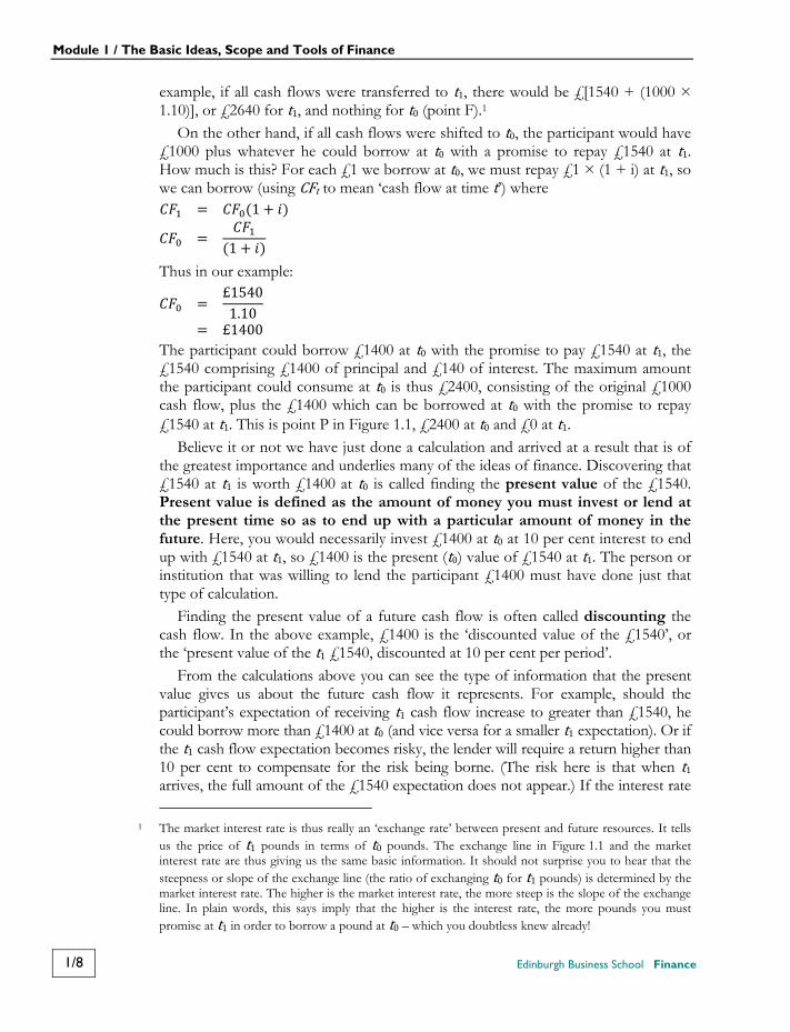
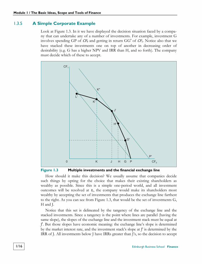
Look at Figure 1.3. In it we have displayed the decision situation faced by a compa-ny that can undertake any of a number of investments. For example, investment G involves spending GP of CF0 and getting in return GG' of CF1. Notice also that we have stacked these investments one on top of another in decreasing order of desirability (e.g. G has a higher NPV and IRR than H, and so forth). The company must decide which of these to accept.
Figure 1.3 Multiple investments and the financial exchange line
How should it make this decision? We usually assume that companies decide such things by opting for the choice that makes their existing shareholders as wealthy as possible. Since this is a simple one-period world, and all investment outcomes will be resolved at t1, the company would make its shareholders most wealthy by accepting the set of investments that produces the exchange line farthest to the right. As you can see from Figure 1.3, that would be the set of investments G, H and J.
Notice that this set is delineated by the tangency of the exchange line and the stacked investments. Since a tangency is the point where lines are parallel (having the same slope), the slopes of the exchange line and the investment stack must be equal at J'. But those slopes have economic meaning: the exchange line’s slope is determined by the market interest rate, and the investment stack’s slope at J' is determined by the IRR of J. All investments below J have IRRs greater than J’s, so the decision to accept
PGK0
P'
K"
L'
K'
J'
H'
G'
J H
CF1
CF0
Module 1 / The Basic Ideas, Scope and Tools of Finance
Finance Edinburgh Business School 1/17
the investments up to and including the one tangential to the new financial exchange line is the same thing as accepting investments until the IRR of the last one is just equal to (or above) the market interest rate. This is the process that will create the most wealth for shareholders, because it causes the company to accept all investments with average per-period earnings rates (IRRs) greater than what the company’s shareholders can earn on comparable investments in the financial market. (To accept investments until the next has a negative or zero NPV is, of course, to do the same thing.)
‘Not so fast,’ you say. ‘Suppose I were the type of person who preferred t0 to t1 consumption. If I were a shareholder of the company I would be happier if they stopped at investment H or G or even made none at all. Then I would have the highest capacity to consume at t0.’
That, of course, is not true. If the company undertakes no investment, your max-imum t0 consumption is P of CF0. Whereas if the company accepts all of the investments up to and including J, you can consume up to P' of CF0 simply by selling your shares at t0 after the market discovers the astuteness of the company’s investment decisions and adjusts the price of its shares. If you have an aversion to selling, nothing would prevent you from borrowing against those shares at t0 in our frictionless market and getting the same amount P' by that mechanism instead.
‘Fair enough,’ you say. ‘But my sister is also a shareholder of the same company, and her consumption preferences are exactly the reverse of mine. She likes nothing better than to increase her future consumption by reducing her current spending. How is the company going to solve the problem of pleasing both of us?’
The answer is that in a market such as this one, companies face no such problem because shareholders can easily solve it themselves. Your sister would simply avoid selling shares, and reinvest any dividends that the company paid her, either in more shares or in lending. The result would be that she delays present consumption until the future. In essence we are saying that a company in this market need not worry about its shareholders’ consumption preferences; the financial market will allow them to make whatever transactions are necessary to be content with their time pattern of resources. Shareholders with quite different preferences for patterns of consumption can thus be content to own the same company’s shares, and the company need not be concerned about the pattern it chooses in which to pay dividends. The sole task of the company is to maximise the present wealth of its shareholders. The shareholders can then adjust their individual patterns of re-sources by dealing in the financial market.
Suppose that the company mistakenly undertook to please your sister by invest-ing a greater amount at t0, and accepted all investments up to K′. From Figure 1.3 you can readily see that her t0 cash flow would decrease and her t1 increase, which is her preferred pattern. But notice also that were the company to maximise her present wealth by investing only to J′, she could in fact retain the same t0 consump-tion (0K) and increase her t1 consumption to KK′′, thereby increasing her satisfaction.
To review the important ideas we have discussed in this section:
Module 1 / The Basic Ideas, Scope and Tools of Finance
1/18 Edinburgh Business School Finance
1. We distinguished between financial and real asset investments, and argued that because of the competitiveness of financial markets it is (usually) necessary to choose real investments in order to expect wealth to increase by investing.
2. We developed the measure of investment desirability called net present value, as the present value of the amounts by which an investment’s cash flows exceed those of its opportunity cost. We also showed that NPV is equal to the change in the wealth of the participant accepting the investment, and that NPV measures the change in market value of the investor’s wealth.
3. We introduced the measure of investment desirability called internal rate of return, the average per-period earning rate of the money invested. When IRR exceeds the opportunity cost (as a rate) of an investment, the investment will have a positive NPV, and therefore be acceptable.
4. We illustrated how these ideas could apply to the investment decisions of a company in a simple financial market like the one described. The company would accept investments up to the point where the next investment would have a negative NPV or an IRR less than its opportunity cost. The company can ig-nore its shareholders’ preferences for particular patterns of cash flow across time because the financial market allows shareholders to reallocate those resources by borrowing and lending as they see fit. This lets the company concentrate on maximising the present wealth of its shareholders, the result of adhering to the investment evaluation techniques of NPV and IRR in this market. All of these ideas are important introductions to finance for people who will be
dealing with these decisions. As important is the general appreciation that we have gained for what a financial market does: 1. It lets people reallocate resources across time, which provides money for real
investment. 2. It gives very important signals, in terms of market rates of return or interest
rates, about the opportunity costs faced by investors. These rates are used as discount rates for making the real asset investment decisions that are so im-portant to an economy.
1.4 More Realistic Financial Markets The simple financial market we have dealt with to this point has allowed us to discover many important characteristics common to all financial markets. You will probably be surprised by the general applicability to ‘real world’ financial decisions of much that you have already learned. It is nevertheless true that our simple financial market cannot portray some of the features of actual markets and financial decisions that are important to learning finance, and so we shall now begin adding those other features.
1.4.1 Multiple-Period Finance
The financial market until now has been limited to single-period transactions; whenever a financial action was taken at t0, its final result occurred at t1, one period later. Actual financial markets, however, contain real and financial assets with
Module 1 / The Basic Ideas, Scope and Tools of Finance
Finance Edinburgh Business School 1/19
returns spanning more than a single period: you can leave your money in a bank for more than one interest period before taking it out; you can buy bonds that pay interest for decades before they stop (or ‘mature’); and you can invest in corporate equities (ordinary shares) that are expected to continue paying dividends for an indeterminately long period into the future. (Some have been paying for a hundred years or so already.) We must be able to address the questions of how such securi-ties are valued, and how financial decision makers deal with real asset choices when the returns from those real assets cover many periods.
With multiple-period assets generating returns across long periods of time, it must seem at first that real financial markets are terribly complex things with which to contend. And we would be telling less than the absolute truth if we said there are no complications introduced by multiple-period assets in the financial market. But it is true that these complexities introduce few new general concepts and are mostly involved in the calculations that are necessary to describe and value the returns that the assets produce.
Actually, there is one way of looking at multiple-period transactions in the finan-cial market that is almost identical to the way we described the single-period market. When we shifted resources across time in the single-period market, we multiplied by (1 + i) to move a period into the future (accruing interest), and divided by (1 + i) to move one period into the past (discounting). The (1 + i) is effectively an ‘exchange rate’ between t0 and t1 resources. In multiple-period transactions the same type of exchange rate applies to shifting resources between any two time points.
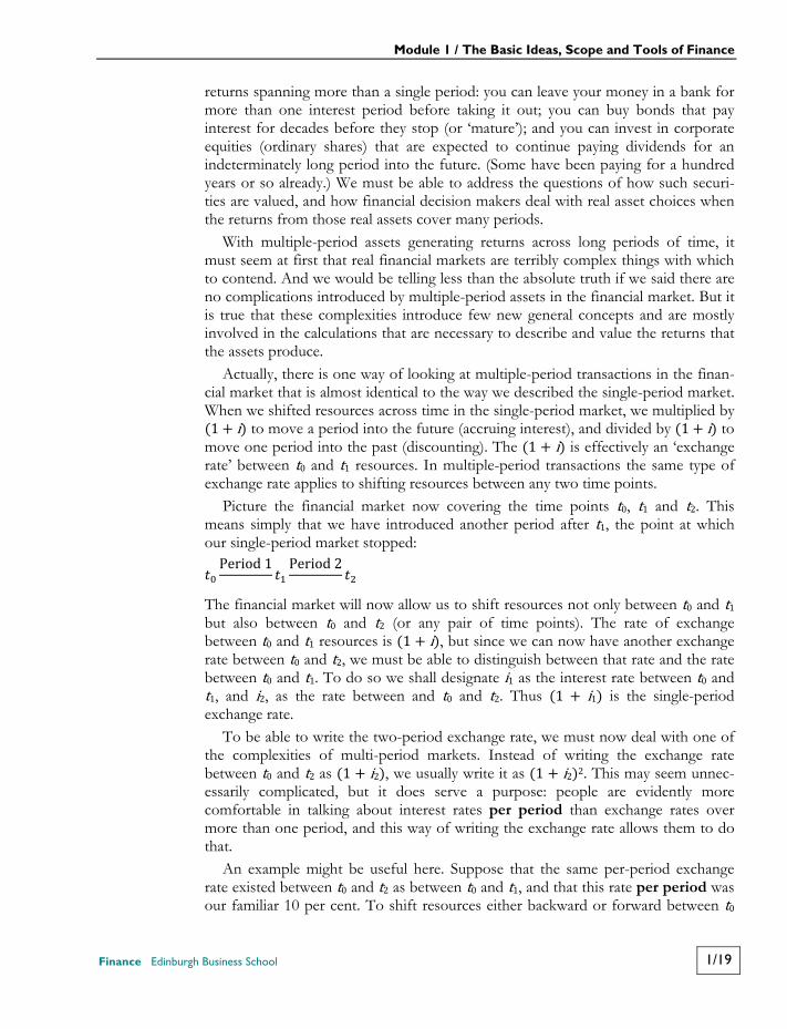
Picture the financial market now covering the time points t0, t1 and t2. This means simply that we have introduced another period after t1, the point at which our single-period market stopped: Period 1 Period 2 The financial market will now allow us to shift resources not only between t0 and t1 but also between t0 and t2 (or any pair of time points). The rate of exchange between t0 and t1 resources is (1 + i), but since we can now have another exchange rate between t0 and t2, we must be able to distinguish between that rate and the rate between t0 and t1. To do so we shall designate i1 as the interest rate between t0 and t1, and i2, as the rate between and t0 and t2. Thus (1 + i1) is the single-period exchange rate.
To be able to write the two-period exchange rate, we must now deal with one of the complexities of multi-period markets. Instead of writing the exchange rate between t0 and t2 as (1 + i2), we usually write it as (1 + i2)2. This may seem unnec-essarily complicated, but it does serve a purpose: people are evidently more comfortable in talking about interest rates per period than exchange rates over more than one period, and this way of writing the exchange rate allows them to do that.
An example might be useful here. Suppose that the same per-period exchange rate existed between t0 and t2 as between t0 and t1, and that this rate per period was our familiar 10 per cent. To shift resources either backward or forward between t0
Module 1 / The Basic Ideas, Scope and Tools of Finance
1/20 Edinburgh Business School Finance
and t1, the exchange rate 1.10 applies. But to shift resources between t0 and t2, we must travel through two periods at the rate 1.10 per period.
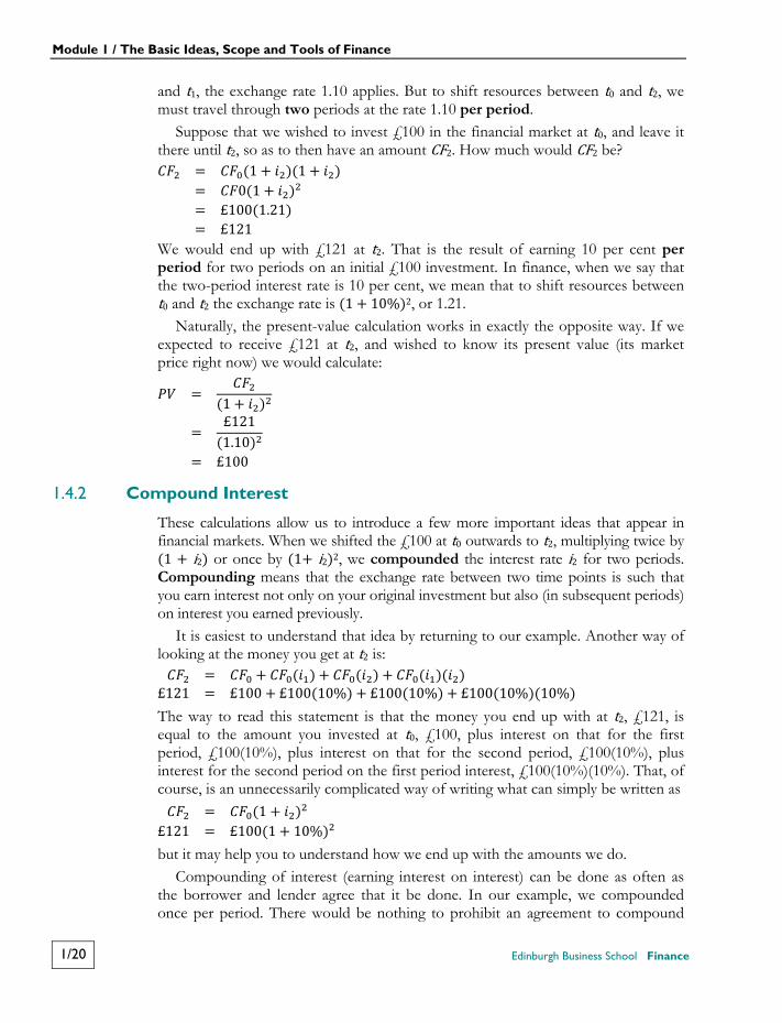
Suppose that we wished to invest £100 in the financial market at t0, and leave it there until t2, so as to then have an amount CF2. How much would CF2 be? = (1 + )(1 + )= 0(1 + )= £100(1.21)= £121 We would end up with £121 at t2. That is the result of earning 10 per cent per period for two periods on an initial £100 investment. In finance, when we say that the two-period interest rate is 10 per cent, we mean that to shift resources between t0 and t2 the exchange rate is (1 + 10%)2, or 1.21.
Naturally, the present-value calculation works in exactly the opposite way. If we expected to receive £121 at t2, and wished to know its present value (its market price right now) we would calculate: = (1 + )= £121(1.10)= £100
1.4.2 Compound Interest
These calculations allow us to introduce a few more important ideas that appear in financial markets. When we shifted the £100 at t0 outwards to t2, multiplying twice by (1 + i2) or once by (1+ i2)2, we compounded the interest rate i2 for two periods. Compounding means that the exchange rate between two time points is such that you earn interest not only on your original investment but also (in subsequent periods) on interest you earned previously.
It is easiest to understand that idea by returning to our example. Another way of looking at the money you get at t2 is: = + ( ) + ( ) + ( )( )£121 = £100 + £100(10%) + £100(10%) + £100(10%)(10%) The way to read this statement is that the money you end up with at t2, £121, is equal to the amount you invested at t0, £100, plus interest on that for the first period, £100(10%), plus interest on that for the second period, £100(10%), plus interest for the second period on the first period interest, £100(10%)(10%). That, of course, is an unnecessarily complicated way of writing what can simply be written as = (1 + )£121 = £100(1 + 10%) but it may help you to understand how we end up with the amounts we do.
Compounding of interest (earning interest on interest) can be done as often as the borrower and lender agree that it be done. In our example, we compounded once per period. There would be nothing to prohibit an agreement to compound
Module 1 / The Basic Ideas, Scope and Tools of Finance
Finance Edinburgh Business School 1/21
twice, three or even more times per period. If the interest rate stays the same, the money amounts would be different because of the number of times interest was compounded between time points.
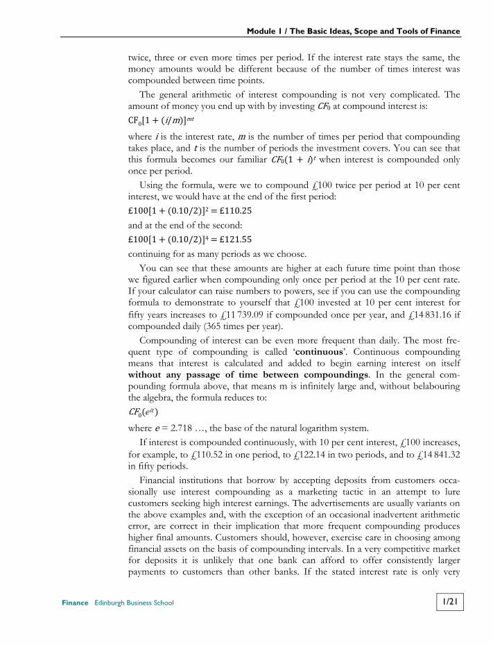
The general arithmetic of interest compounding is not very complicated. The amount of money you end up with by investing CF0 at compound interest is: CF0[1 + (i/m)]mt where i is the interest rate, m is the number of times per period that compounding takes place, and t is the number of periods the investment covers. You can see that this formula becomes our familiar CF0(1 + i)t when interest is compounded only once per period.
Using the formula, were we to compound £100 twice per period at 10 per cent interest, we would have at the end of the first period: £100[1 + (0.10/2)]2 = £110.25 and at the end of the second: £100[1 + (0.10/2)]4 = £121.55 continuing for as many periods as we choose.
You can see that these amounts are higher at each future time point than those we figured earlier when compounding only once per period at the 10 per cent rate. If your calculator can raise numbers to powers, see if you can use the compounding formula to demonstrate to yourself that £100 invested at 10 per cent interest for fifty years increases to £11 739.09 if compounded once per year, and £14 831.16 if compounded daily (365 times per year).
Compounding of interest can be even more frequent than daily. The most fre-quent type of compounding is called ‘continuous’. Continuous compounding means that interest is calculated and added to begin earning interest on itself without any passage of time between compoundings. In the general com-pounding formula above, that means m is infinitely large and, without belabouring the algebra, the formula reduces to: CF0(eit ) where e = 2.718 …, the base of the natural logarithm system.
If interest is compounded continuously, with 10 per cent interest, £100 increases, for example, to £110.52 in one period, to £122.14 in two periods, and to £14 841.32 in fifty periods.
Financial institutions that borrow by accepting deposits from customers occa-sionally use interest compounding as a marketing tactic in an attempt to lure customers seeking high interest earnings. The advertisements are usually variants on the above examples and, with the exception of an occasional inadvertent arithmetic error, are correct in their implication that more frequent compounding produces higher final amounts. Customers should, however, exercise care in choosing among financial assets on the basis of compounding intervals. In a very competitive market for deposits it is unlikely that one bank can afford to offer consistently larger payments to customers than other banks. If the stated interest rate is only very
Module 1 / The Basic Ideas, Scope and Tools of Finance
1/22 Edinburgh Business School Finance
slightly lower than one compounded less frequently, the difference may nevertheless offset any compounding benefit. Or some non-monetary dimension of service may be different.
We must always remember that financial market participants consume money resources, not interest rates or compounding intervals; they make their comparisons of desirability on the basis of money-measured values. They cannot be fooled into thinking, for example, that continuous compounding is necessarily better than no compounding, unless they are also informed of the interest rates to be compounded. Nor will they assume that lending money at a rate of 10.1 per cent is necessarily better than lending at 10 per cent, if the two rates are not identically compounded.
For the remainder of the course we shall adopt the common convention that, unless told otherwise, interest is compounded once per period.
1.4.3 Multiple-Period Cash Flows
Extending the financial market to cover any number of periods is now easily within our reach. Suppose that you expect to receive a cash flow at t3 and are curious about its present value. If you know that your average three-period opportunity cost is i3 per period, the present value of the t3 cash flow is: = (1 + )
The same general procedure will allow us to find the present value of a cash flow occurring at any future time point. Where t can be any time, the general method for finding the present value of any cash flow is: = (1 + ) Moving in the other direction, the future value of a present amount invested at the rate it for t periods is, of course, the invested amount multiplied by (1 + it)t.
The securities and assets in multiple-period financial markets often have more than a single cash flow expected for the future. Usually a corporate bond or an ordinary share (equity) is expected to pay several cash amounts as interest, principal or dividends at several times in the future. Similarly, a real asset investment, such as a new piece of machinery or going into a new line of business, almost always has cash flows expected for many periods. How does finance deal with valuing such cash flows?
We follow the same rules that we have used thus far, while merely combining the cash flow present values. For example, suppose that we are interested in the present value of a set (we call this a ‘stream’) of cash flows that comprises £100 at each of t1, t2 and t3, and our opportunity costs are all 10 per cent per period:
Module 1 / The Basic Ideas, Scope and Tools of Finance
Finance Edinburgh Business School 1/23
= (1 + ) + (1 + ) + (1 + )= £100(1.10) + £100(1.10) + £100(1.10)= £100(1.10) + £100(1.21) + £100(1.331)= £90.91 + £82.65 + £75.13= £248.69
The present value of the stream of cash flows is £248.69, being the sum of the present values of the future cash flows in the stream. Though the arithmetic of this example is quite rudimentary, the economic lesson it portrays is important. It tells us that the correct way to view the value of an asset that generates a stream of future cash flows is as the sum of the present values of each of the future cash flows associated with the asset.
1.4.4 Multiple-Period Investment Decisions
Earlier we introduced two investment decision-making techniques that are con-sistent with present wealth maximisation in financial markets. We shall now illustrate the basics of how these techniques, NPV and IRR, operate in multiple-period asset evaluations.
Calculating NPV when the investment decision will affect several future cash flows is no more difficult than any multiple-period present value calculation. We need simply to remember that NPV must include all present and future cash flows associated with the investment. For example, suppose that the stream we valued in the section immediately above is the set of future cash flows of an investment with a t0 cash outlay of £200. Combining all of the present values of the investment’s cash flows produces an NPV of £48.69, which is the net of £248.69 (the present value of future cash flows) minus £200 (the present value of the present cash flow): NPV = + (1 + ) + (1 + ) + (1 + )= −£200 + £100(1.10) + £100(1.10) + £100(1.10)= −£200 + £100(1.10) + £100(1.21) + £100(1.331)= −£200 + £90.91 + £82.65 + £75.13= +£48.69
Finding the IRR of a set of cash flows that extends across several future periods
is more complicated than calculating its NPV. Remember that IRR is the discount rate that causes the present value of all cash flows (NPV) to equal zero. In the example we are working on, the following equation for IRR must be solved: 0 = + (1 + IRR) + (1 + IRR) + (1 + IRR)= −£200 + £100(1 + IRR) + £100(1 + IRR) + £100(1 + IRR)
Module 1 / The Basic Ideas, Scope and Tools of Finance
1/24 Edinburgh Business School Finance
In terms of the mathematics involved, there is no general formula that will allow us to solve all such IRR equations. Instead, the way we solve for the IRR of a multiple-period cash flow stream is with a technique called ‘trial and error’. This means we choose some arbitrary discount rate for IRR in the above equation, and calculate NPV. We then examine the result to decide whether the rate we used was too high or too low, choose another rate that appears to be better than the one we just used, and again calculate NPV. We continue this process until we find the IRR (or as close an approximation to it as seems necessary) that creates an NPV equal to zero.
Suppose that we first try 15 per cent as a potential IRR: NPV = −£200 + £100(1.15) + £100(1.15) + £100(1.15)= +£28.32 A 15 per cent discount rate produces an NPV greater than zero, so 15 per cent is
not the IRR of the cash flows. Since the NPV is too large, we should probably choose a higher discount rate (since increases in the discount rate, being in the denominator, will cause a lower NPV for these cash flows). Let us try 25 per cent: NPV = −£200 + £100(1.25) + £100(1.25) + £100(1.25)= −£4.80
A 25 per cent discount rate yields a small but negative NPV, and so 25 per cent is too large. Nevertheless, we have discovered that the IRR of the cash flows is somewhere between 15 and 25 per cent because the former yields a positive and the latter a negative NPV. To find the true IRR, we continue this search process until we find the exact IRR, become convinced that the range we have found is suffi-ciently accurate for the decision at hand, or run out of patience.
The actual IRR for this example is 23.4 per cent per period, implying that, be-cause IRR exceeds the 10 per cent opportunity cost, the investment is acceptable. Actually, we could have decided that as soon as we saw a positive NPV at a 15 per cent discount rate, since we knew thereby that the IRR was greater than 15 per cent. With an opportunity cost of 10 per cent and an IRR greater than 15 per cent we have enough information to decide that the investment is desirable.
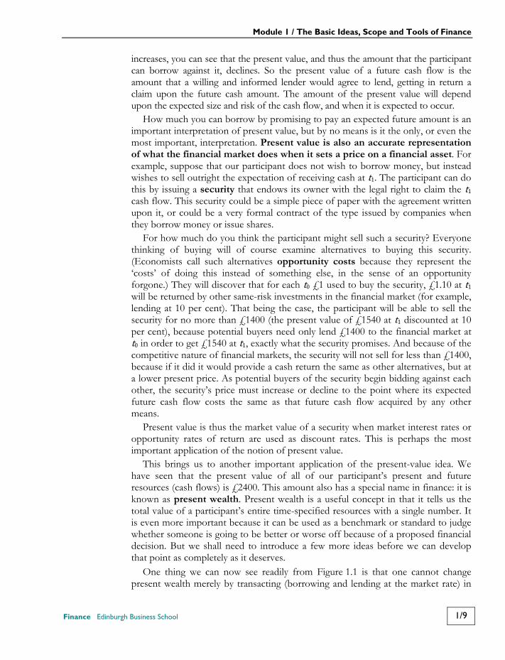
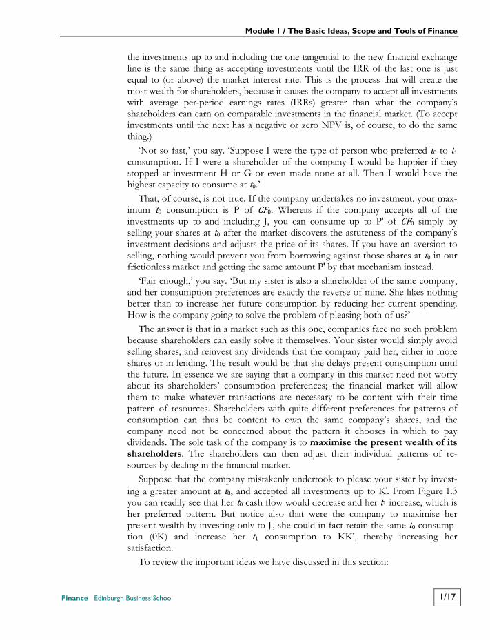
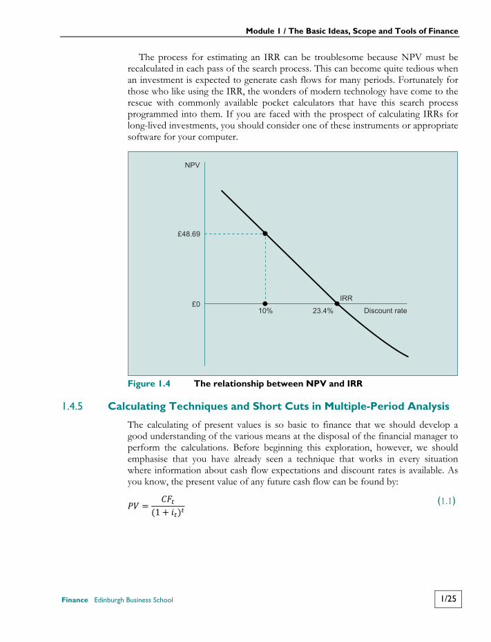
Figure 1.4 should be helpful in visualising the method of finding the IRR. Note that the vertical axis of the figure records NPV, and the horizontal axis plots the discount rates used to calculate NPV. The curve indicates that, in the example we are examining, as the discount rate increases, NPV declines. (This is a very common relationship between NPV and its discount rates. As long as cash outflows tend to be closer to the present than cash inflows from an investment, we usually see a curve that looks like this one.) The search for an IRR is easy to visualise in Figure 1.4. If your first try uses a rate less than 23.4 per cent, the NPV will be positive; if more, it will be negative. If you get a positive NPV, you should try a rate higher than the one you have used; if you get a negative NPV, you should try a lower one. Eventually you will narrow the search to a rate that creates an NPV nearly equal to zero, and that rate will be the IRR.
Module 1 / The Basic Ideas, Scope and Tools of Finance
Finance Edinburgh Business School 1/25
The process for estimating an IRR can be troublesome because NPV must be recalculated in each pass of the search process. This can become quite tedious when an investment is expected to generate cash flows for many periods. Fortunately for those who like using the IRR, the wonders of modern technology have come to the rescue with commonly available pocket calculators that have this search process programmed into them. If you are faced with the prospect of calculating IRRs for long-lived investments, you should consider one of these instruments or appropriate software for your computer.
Figure 1.4 The relationship between NPV and IRR
1.4.5 Calculating Techniques and Short Cuts in Multiple-Period Analysis
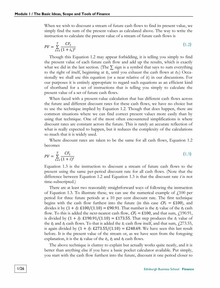
The calculating of present values is so basic to finance that we should develop a good understanding of the various means at the disposal of the financial manager to perform the calculations. Before beginning this exploration, however, we should emphasise that you have already seen a technique that works in every situation where information about cash flow expectations and discount rates is available. As you know, the present value of any future cash flow can be found by: = (1 + ) ﴾1.1﴿
NPV
£48.69
£010% 23.4%
IRR
Discount rate
Module 1 / The Basic Ideas, Scope and Tools of Finance
1/26 Edinburgh Business School Finance
When we wish to discount a stream of future cash flows to find its present value, we simply find the sum of the present values as calculated above. The way to write the instruction to calculate the present value of a stream of future cash flows is = ∑ (1 + ) ﴾1.2﴿
Though this Equation 1.2 may appear forbidding, it is telling you simply to find the present value of each future cash flow and add up the results, which is exactly what we did in the last section. (The ∑ sign is a symbol that says to sum everything to the right of itself, beginning at t1, until you exhaust the cash flows at tT.) Occa-sionally we shall use this equation (or a near relative of it) in our discussions. For our purposes it is entirely appropriate to regard such equations as an efficient kind of shorthand for a set of instructions that is telling you simply to calculate the present value of a set of future cash flows.
When faced with a present-value calculation that has different cash flows across the future and different discount rates for these cash flows, we have no choice but to use the technique implied by Equation 1.2. Though that does happen, there are common situations where we can find correct present values more easily than by using that technique. One of the most often encountered simplifications is where discount rates are constant across the future. This is rarely an accurate reflection of what is really expected to happen, but it reduces the complexity of the calculations so much that it is widely used.
Where discount rates are taken to be the same for all cash flows, Equation 1.2 becomes = ∑ (1 + ) ﴾1.3﴿
Equation 1.3 is the instruction to discount a stream of future cash flows to the present using the same per-period discount rate for all cash flows. (Note that the difference between Equation 1.2 and Equation 1.3 is that the discount rate i is not time-subscripted.)
There are at least two reasonably straightforward ways of following the instruction of Equation 1.3. To illustrate these, we can use the numerical example of £100 per period for three future periods at a 10 per cent discount rate. The first technique begins with the cash flow furthest into the future (in this case CF3 = £100), and divides it by (1 + i): £100/(1.10) = £90.91. That number is the t2 value of the t3 cash flow. To this is added the next-nearest cash flow, CF2 = £100, and that sum, £190.91, is divided by (1 + i): £190.91/(1.10) = £173.55. That step produces the t1 value of the t2 and t3 cash flows. To that is added the t1 cash flow itself, and that sum, £273.55, is again divided by (1 + i): £273.55/(1.10) = £248.69. We have seen this last result before. It is the present value of the stream or, as we have seen from the foregoing explanation, it is the t0 value of the t1, t2 and t3 cash flows.
The above technique is clumsy to explain but actually works quite neatly, and it is better than anything else if you have a basic pocket calculator available. Put simply, you start with the cash flow furthest into the future, discount it one period closer to
Module 1 / The Basic Ideas, Scope and Tools of Finance
Finance Edinburgh Business School 1/27
the present, add the cash flow from that closer time point, and discount that sum one period nearer to the present; you continue that process until all cash flows are included, and discounted back to t0.
Another commonly used technique of finding present values relies on present value tables. Present value tables are simply lists of actual values of Equation 1.1 and Equation 1.3, with 1 as the cash flow in the numerators of the equations, and with present values calculated for a wide range of time points, stream lengths and discount rates. Present value tables therefore give the present values per pound of future cash flow, either for a single cash flow (Equation 1.1) or a stream of constant cash flows discounted at constant discount rates (Equation 1.3). We have included a set of these tables in Appendix 1.
To illustrate the use of the tables, turn to Table A1.1 in Appendix 1, which shows the present value of £1 to be received at time point t. Note that in the column for a 10 per cent discount, the factors for the first three time points are indicated as 0.9091, 0.8264, and 0.7513 respectively. To find the present value of our £100 per period for three periods, we multiply each of these factors by the £100 cash flow occurring at its time point, and add up the result. The answer is, of course, £248.69 (actually the result is £0.01 less because of rounding).
Using present value tables for such calculations is unnecessary since the calcula-tor technique above has the same number of steps and does not use the tables. There are, however, instances where the tables are efficient. One obvious example is in calculating the present value of a single cash flow located far into the future when your calculator cannot perform exponentiation (i.e. raising numbers to powers). You would not enjoy dividing £100 by (1.10) twenty times if your calculator could not figure (1.10)20 directly. Table A1.1 tells you that £1/(1.10)20 is 0.1486, and there-fore that the value of £100 to be received at t20 is £14.86 at t0 with a discount rate of 10 per cent.
Another circumstance when the tables are useful is in finding the present value of annuities. A constant annuity is a set of cash flows that are the same amounts across future time points. Such a present value is calculated with our Equation 1.3, but with no subscript on the cash flows since they are all the same. Since Table A1.2 in Appendix 1 gives the present value of £1 per period for t periods, it implies a constant cash flow per period and is therefore an annuity table. To illustrate its use, note that under the column for 10 per cent discount, the three-period annuity factor is listed as 2.4869. It takes little effort to see that with £100 per period for three periods, we arrive at our familiar answer, £248.69. When annuities run for many periods, the use of this table rather than a calculator is wise (unless you own one of the sophisticated devices programmed to do such calculations directly).3
3 Cash flows can, of course, be invested at interest to produce future amounts of cash. Table A1.3
and Table A1.4 in Appendix 1 are the future value counterparts of Table A1.1 and Table A1.2 in the same Appendix. In addition to the tables and pocket calculators with built-in financial functions, all current personal computer spreadsheet programs have these (and many more) financial formulas able to be called up as automatic functions. You should not hesitate to use such spreadsheets instead of the tables or calculators if you feel comfortable doing so. Because of the increasingly common availability
Module 1 / The Basic Ideas, Scope and Tools of Finance
1/28 Edinburgh Business School Finance
We mentioned earlier that some of the assets commonly valued in finance have cash-flow expectations that extend very far into the future. When faced with cash flows of that nature, there is yet another technique of present value calculation that is often used in financial practice: the perpetuity. A perpetuity is a cash flow stream that is assumed to continue for ever. Perpetuity present values are used because they are so easy to calculate. The formula for the present value of a perpetuity is: = ﴾1.4﴿
To find the present value of a perpetuity one merely divides the (constant) per-period cash flow by the (constant) per-period discount rate. This means, for example, that £100 per period for ever at a discount rate of 10 per cent has a present value of £100/0.10 = £1000. (It is intuitively easy to see why this formula works. Another way of saying the same thing is that if you put £1000 in the bank at 10 per cent interest, you can take out £100 per year for ever.)
The ease of calculation of perpetuities is attractive. Not so attractive is the as-sumption that the cash-flow stream will continue for ever. Obviously, no asset is actually likely to continue producing cash flows for ever, but before you become offended that financial practitioners use a technique that makes such a ridiculous assumption, let us test whether or not the answers it gives are ridiculous.
Suppose that you are faced with valuing a stream of £100 cash flows with 10 per cent opportunity costs, and the stream is expected to continue very far into the future but you are not exactly sure how far. Were you to use an admittedly incorrect perpetuity value, it would be £100/0.10 = £1000. How large an error are you likely to be making by using that value?
Suppose that the cash flows are unlikely to last much beyond forty periods. With a discount rate of 10 per cent, £100 in the fortieth year has a present value of only £2.21 = £100/(1.10)40. As a matter of fact, the total present value of all cash flows from the fortieth year until the end of time is only (£100/0.10)/(1.10)40 = £22.10. This means that by using a perpetuity valuation, even if the stream actually ends in the fortieth year instead of continuing for ever, the value error is £22.10 out of £1000, or 2.21 per cent. As we shall see in our study of uncertainty, other errors in making cash-flow estimates are likely to be large enough so as to overshadow mistakes of this magnitude in present-value calculations. Of course, the size of the error is a function of when the actual cash flow would cease, and could be much larger than 2 per cent. For example, if the cash flow were to cease in the twentieth year, the error in using the £1000 perpetuity value would be £1000/(1.10)20 = £148.64, and a 14.9 per cent error may be too large to be tolerable.
Though perpetuity valuation can be convenient and may not err greatly in long-lived assets, Equation 1.4 also assumes that the cash flows will be constant for each future period. That is not very representative of actual patterns of cash flows that we see. Fortunately there is a slight modification of Equation 1.4 which can make it
of these spreadsheets (with the computers to use them) and their inherent power and flexibility, if you have not made the decision to begin using one, now might be a good time to consider doing so.
Module 1 / The Basic Ideas, Scope and Tools of Finance
Finance Edinburgh Business School 1/29
a bit more useful without significantly altering its simplicity. If we assume that the cash flows will continue for ever, but will grow or decline at a constant percentage rate during each period, the perpetuity formula becomes = ( − ) ﴾1.5﴿
where g is the constant per-period growth rate of the cash flow. For example, suppose that we must value a cash-flow stream that begins at the
end of this period with £100, but that will grow at a rate of 5 per cent per period every period thereafter (such that there will be a cash inflow of £105 at t2, of £110.25 at t3, and so forth, for ever). With a discount rate of 10 per cent, the value of the stream is: = £100(0.10 − 0.05) = £2000 (The ‘bank account’ intuition here is like that of the constant perpetuity, except that your withdrawals grow each year at 5 per cent.)
This ‘growth perpetuity’ present-value calculation is widely used for several fi-nancial applications, especially when investigating the values of long-lived organisations like large modern corporations. One note of caution, however: the equation obviously does not work when the discount rate i is less than or equal to the growth rate g. The implication that a cash flow, growing for ever at a rate nearly equal to its opportunity cost, has an infinitely high present value, is numerically correct, but not economically useful, because it could not reasonably be expected to happen.
Since this has been a rather long section, we should review the points we have developed in it. In discussing the various techniques that finance uses to perform discounting calculations we have discovered that: 1. There is a simple calculator-based technique that is very effective for valuing
cash-flow streams that run for only a few periods. 2. When the stream continues for several periods and has the same cash flow for
each period, annuity present-value tables (giving the present value of £1 per period) can be used.
3. When cash flows are well into the future, and the calculator being used cannot exponentiate, single-cash-flow present-value tables (‘present value of £1’) are useful.
4. Some financial pocket calculators can do all of the above with pre-programmed ease. The spreadsheet programs widely available on personal computers have financial functions that are even easier to use, more flexible and more powerful than sophisticated pocket calculators.
5. Perpetuities, either constant or growing (or even declining) by a constant percentage per period, can often be used as reasonable approximations for cash-flow streams from very long-lived assets.
Module 1 / The Basic Ideas, Scope and Tools of Finance
1/30 Edinburgh Business School Finance
With enough practice, some of which is provided by the exercises at the end of Module 1, you will quickly come to recognise the particular situation in which each technique is most efficient.
1.5 Interest Rates, Interest Rate Futures and Yields In this section we shall develop more fully some ideas about interest rates that we introduced in earlier sections. You probably feel as if you have heard enough about interest rates to last you a lifetime, but there are a few additional concepts involved in their use that we have been holding back until our multiple-period framework was complete. The first set of these ideas concerns itself with forward or future interest rates, and something called the ‘term structure’ of interest rates. In our discussion of these topics we shall also learn a few important things about the debt securities called bonds.
When we first discussed interest rates we said that the best way to understand them was as ratios or ‘rates of exchange’ used when shifting resources across time. We would now like to consider the idea that such exchanges or interest rates can take place not only between now and some future time point but also between any two time points, present or future. In other words, if there is an interest rate that applies between t0 and t2, there could also be one between t1 and t2, or between t2 and t6, or any other combination. Hearing this proposal, your reaction is probably that such rates may be conceptually fine, but (1) would be of little use because no one ever borrows or lends with such rates, and (2) like most academics we are unnecessarily trying to make an already complicated system even more complex.
We would be the first to admit that academics are often attracted to complexity for its own sake (it encourages the consumers of our product to think that we are uniquely able to produce it). But that is not the case with this interest-rate discus-sion. There are large and active markets today that do in fact effectively borrow and lend between future time points, and therefore cause such rates to exist and be observed. Such transactions are increasingly important in a wide range of financial decisions made by sophisticated modern organisations. Equally importantly, the concept of interest rates between future time points also allows us to understand much more about everyday securities (such as the bonds our governments issue) than we could without this idea.
To illustrate some of the important relationships in this market, suppose that five securities, A to E, are traded in this market and have future cash-flow expectations as listed in Table 1.1 for time points t1 to t3. Further, suppose that the securities’ cash flows are riskless, and that the per-period interest rates that would apply are 5 per cent for the first period (between t0 and t1), 6 per cent for the two-period rate (between t0 and t2), and 7 per cent for the three-period rate (between t0 and t3). Incidentally, in financial markets, interest rates that begin at the present and run to some future time point are called spot interest rates. So another way of saying what we have just said is that the one-period spot rate is 5 per cent, the two-period spot rate is 6 per cent, and the three-period spot rate is 7 per cent.
The set of all spot rates in a financial market is called the term structure of interest rates. With those rates, we can easily calculate the present values (or market
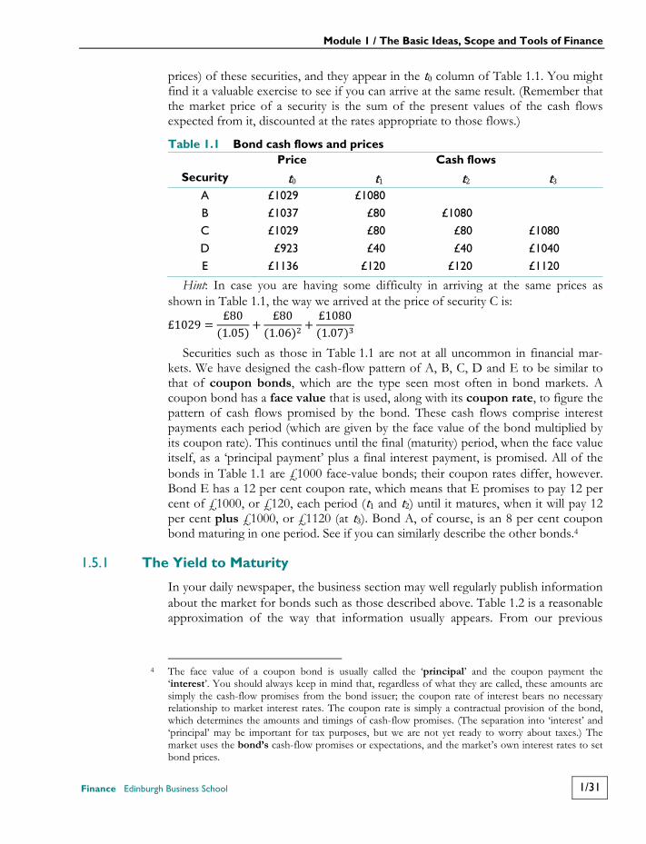
Module 1 / The Basic Ideas, Scope and Tools of Finance
Finance Edinburgh Business School 1/31
prices) of these securities, and they appear in the t0 column of Table 1.1. You might find it a valuable exercise to see if you can arrive at the same result. (Remember that the market price of a security is the sum of the present values of the cash flows expected from it, discounted at the rates appropriate to those flows.)
Table 1.1 Bond cash flows and prices Price Cash flows
Security t0 t1 t2 t3 A £1029 £1080
B £1037 £80 £1080
C £1029 £80 £80 £1080
D £923 £40 £40 £1040
E £1136 £120 £120 £1120
Hint: In case you are having some difficulty in arriving at the same prices as shown in Table 1.1, the way we arrived at the price of security C is: £1029 = £80(1.05) + £80(1.06) + £1080(1.07)
Securities such as those in Table 1.1 are not at all uncommon in financial mar-kets. We have designed the cash-flow pattern of A, B, C, D and E to be similar to that of coupon bonds, which are the type seen most often in bond markets. A coupon bond has a face value that is used, along with its coupon rate, to figure the pattern of cash flows promised by the bond. These cash flows comprise interest payments each period (which are given by the face value of the bond multiplied by its coupon rate). This continues until the final (maturity) period, when the face value itself, as a ‘principal payment’ plus a final interest payment, is promised. All of the bonds in Table 1.1 are £1000 face-value bonds; their coupon rates differ, however. Bond E has a 12 per cent coupon rate, which means that E promises to pay 12 per cent of £1000, or £120, each period (t1 and t2) until it matures, when it will pay 12 per cent plus £1000, or £1120 (at t3). Bond A, of course, is an 8 per cent coupon bond maturing in one period. See if you can similarly describe the other bonds.4
1.5.1 The Yield to Maturity
In your daily newspaper, the business section may well regularly publish information about the market for bonds such as those described above. Table 1.2 is a reasonable approximation of the way that information usually appears. From our previous
4 The face value of a coupon bond is usually called the ‘principal’ and the coupon payment the
‘interest’. You should always keep in mind that, regardless of what they are called, these amounts are simply the cash-flow promises from the bond issuer; the coupon rate of interest bears no necessary relationship to market interest rates. The coupon rate is simply a contractual provision of the bond, which determines the amounts and timings of cash-flow promises. (The separation into ‘interest’ and ‘principal’ may be important for tax purposes, but we are not yet ready to worry about taxes.) The market uses the bond’s cash-flow promises or expectations, and the market’s own interest rates to set bond prices.
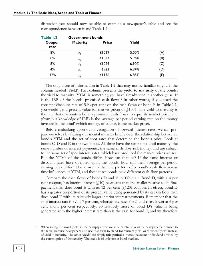
Module 1 / The Basic Ideas, Scope and Tools of Finance
1/32 Edinburgh Business School Finance
discussion you should now be able to examine a newspaper’s table and see the correspondence between it and Table 1.2.
Table 1.2 Government bonds Coupon
rate Maturity Price Yield
8% £1029 5.00% (A)
8% £1037 5.96% (B)
8% £1029 6.90% (C)
4% £923 6.94% (D)
12% £1136 6.85% (E)
The only piece of information in Table 1.2 that may not be familiar to you is the column headed ‘Yield’. That column presents the yield to maturity of the bonds; the yield to maturity (YTM) is something you have already seen in another guise. It is the IRR of the bonds’ promised cash flows.5 In other words, if you used the constant discount rate of 5.96 per cent on the cash flows of bond B in Table 1.1, you would get a present value (or market price) of £1037. The yield to maturity is the rate that discounts a bond’s promised cash flows to equal its market price, and (from our knowledge of IRR) is the ‘average per-period earning rate on the money invested in the bond’ (which money, of course, is the market price).
Before embarking upon our investigation of forward interest rates, we can pre-pare ourselves by flexing our mental muscles briefly over the relationship between a bond’s YTM and the set of spot rates that determine the bond’s price. Look at bonds C, D and E in the two tables. All three have the same time until maturity, the same number of interest payments, the same cash-flow risk (none), and are subject to the same set of spot interest rates, which have produced the market prices we see. But the YTMs of the bonds differ. How can that be? If the same interest or discount rates have operated upon the bonds, how can their average per-period earning rates differ? The answer is that the pattern of a bond’s cash flow across time influences its YTM, and these three bonds have different cash-flow patterns.
Compare the cash flows of bonds D and E in Table 1.1. Bond D, with a 4 per cent coupon, has interim interest (£40) payments that are smaller relative to its final payment than does bond E with its 12 per cent (£120) coupon. In effect, bond D has a greater proportion of its present value being generated by its t3 cash flow than does bond E with its relatively larger interim interest payments. Remember that the spot interest rate for t3 is 7 per cent, whereas the rates for t2 and t1 are lower at 6 per cent and 5 per cent respectively. So relatively more of bond D’s value is being generated with the higher interest rate than is the case for bond E, and we therefore
5 When seeing the word ‘yield’ in the newspaper you must be careful to read the newspaper’s footnote to
the table, because newspapers also use that term to stand for ‘current yield’ or ‘dividend yield’ instead of yield to maturity. The other ‘yields’ are simply this period’s interest payment or dividend divided by the current price of the security. That ratio is of little use in bond markets.
Module 1 / The Basic Ideas, Scope and Tools of Finance
Finance Edinburgh Business School 1/33
see a higher per-period earning rate or YTM for D than for E. See if you can convince yourself that bond C’s yield can be similarly explained.
The phenomenon we have described above has a name in finance; it is called the coupon effect on the yield to maturity. It gets this name because the size of the coupon of a bond determines the pattern of its cash flows, and thus how its YTM will reflect the set of spot rates that exists in the market. The YTM is mathematically a very complex average of the spot rates of interest, as weighted by the pattern of cash flows of a bond. Depending upon your attraction to matters mathematical, you will be either pleased or disappointed to hear that at this point it would not benefit us to pursue further this particular aspect of the YTM.
What we have learned about the yield to maturity should teach us to be very careful how we use it. For example, it would be most unwise to make comparisons among securities on the basis of their YTMs unless their patterns of cash flows (coupons, for bonds) were identical. The YTM, being a complex constant per-period average, might lead the uninitiated to think that the money invested in one bond was earning a better or worse rate than another bond in any given period, whereas it is clear that bonds of equal risk must earn the same rates during the same periods. The YTMs are expressing not only the earning rates but also the amounts invested in the bonds across time. In our example, bond E had a lower YTM than bond D because E’s higher interim cash interest payments meant that relatively less was invested at the later periods (which had the higher interest rates).
Occasionally you may see the yield curve referenced as synonymous with the term structure of interest rates. The former is the set of YTMs that exists in the market, usually for government coupon bonds. The latter is, as we know, the set of spot interest rates. From what you now know about interest rates, you should be uncomfortable with using the yield curve as a substitute for the term structure.
1.5.2 Forward Interest Rates
We are now ready to discuss the set of interest rates that begin at some time point other than t0 (now), and hence cannot be spot rates. As we mentioned earlier, these are called forward rates because of their location forward in time. Look at bond B in Table 1.1 and Table 1.2. The t0 investor in bond B spends £1037 in order to get £80 at t1 and £1080 at t2. The spot rates tell us that the £1037 t0 value of these cash flows can be regarded as:6 = (1 + ) + (1 + )= £80(1.05) + £1080(1.06)= £76 + £961= £1037
6 For simplicity of presentation we have selectively rounded off the cash flows, values and rates in this section. If you prefer numbers of higher accuracy, and if your calculator runs to several decimal places, we encourage you to investigate the more accurate results. To have the results consistent, you can assume that the spot rates, coupons and face amounts above are exact, and all other values and rates produced herein are rounded.
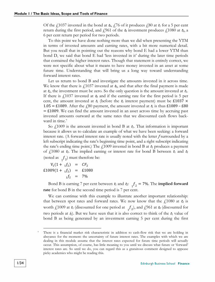
Module 1 / The Basic Ideas, Scope and Tools of Finance
1/34 Edinburgh Business School Finance
Of the £1037 invested in the bond at t0, £76 of it produces £80 at t1 for a 5 per cent return during the first period, and £961 of the t0 investment produces £1080 at t2, a 6 per cent return per period for two periods.
To this point we have done nothing more than we did when presenting the YTM in terms of invested amounts and earning rates, with a bit more numerical detail. But you recall that in pointing out the reasons why bond E had a lower YTM than bond D, we said that bond E had ‘less invested in it’ during the later time periods that contained the higher interest rates. Though that statement is entirely correct, we were not specific about what it means to have money invested in an asset at some future time. Understanding that will bring us a long way toward understanding forward interest rates.
Let us return to bond B and investigate the amounts invested in it across time. We know that there is £1037 invested at t0, and that after the final payment is made at t2, the investment must be zero. So the only question is the amount invested at t1. If there is £1037 invested at t0 and if the earning rate for the first period is 5 per cent, the amount invested at t1 (before the t1 interest payment) must be £1037 × 1.05 = £1089. After the £80 payment, the amount invested at t1 is thus £1089 – £80 = £1009. We can find the amount invested in an asset across time by accruing past invested amounts outward at the same rates that we discounted cash flows back-ward in time.7
So £1009 is the amount invested in bond B at t1. That information is important because it allows us to calculate an example of what we have been seeking: a forward interest rate. (A forward interest rate is usually noted with the letter ƒ surrounded by a left subscript indicating the rate’s beginning time point, and a right subscript indicating the rate’s ending time point.) The £1009 invested in bond B at t1 produces a payment of £1080 at t2. The implied earning or interest rate for bond B between t1 and t2 (noted as 21 ) must therefore be: V (1 + ) =£1009(1 + ) = £1080= 7%
Bond B is earning 7 per cent between t1 and t2: 21 = 7%. The implied forward rate for bond B in the second time period is 7 per cent.
We can continue with this example to illustrate another important relationship: that between spot rates and forward rates. We now know that the £1080 at t2 is worth £1009 at t1 (discounted for one period at 21 ), and £961 at t0 (discounted for two periods at i2). But we have seen that it is also correct to think of the t1 value of bond B as being generated by an investment earning 5 per cent during the first
7 There is a financial market risk characteristic in addition to cash-flow risk that we are holding in
abeyance for the moment: the uncertainty of future interest rates. The examples with which we are dealing in this module assume that the interest rates expected for future time periods will actually occur. This assumption, of course, has little meaning to you until we discuss what future or ‘forward’ interest rates are. So until we do, you can regard this as a gratuitous comment designed to appease picky academics who might be reading this.
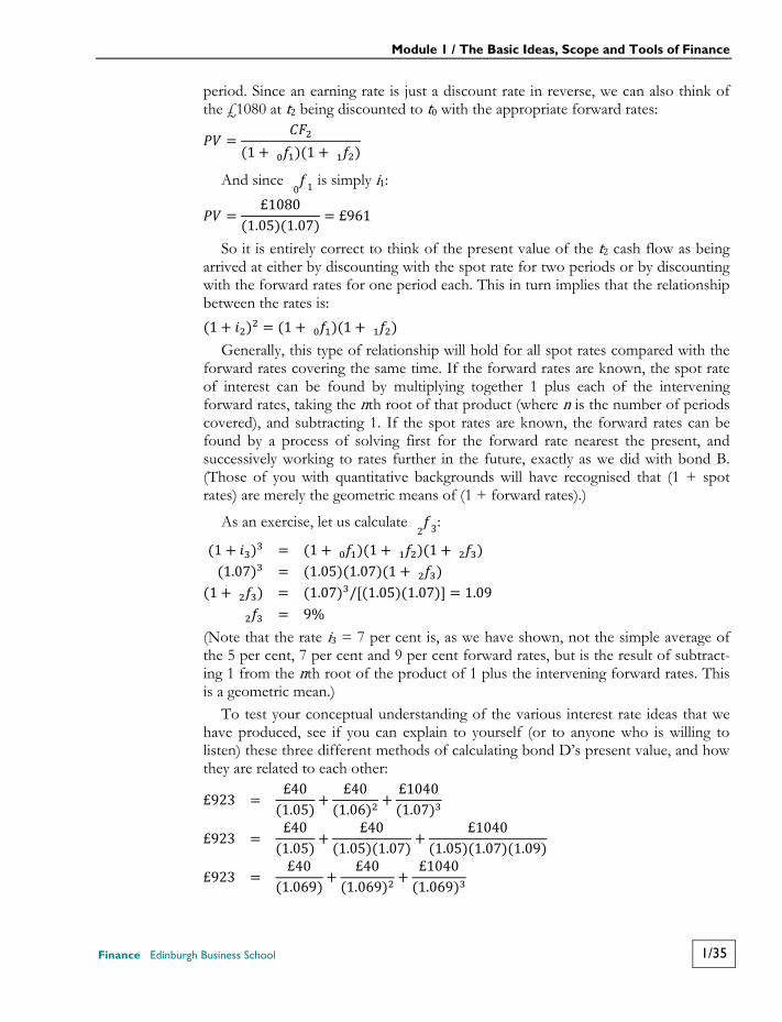
Module 1 / The Basic Ideas, Scope and Tools of Finance
Finance Edinburgh Business School 1/35
period. Since an earning rate is just a discount rate in reverse, we can also think of the £1080 at t2 being discounted to t0 with the appropriate forward rates: = (1 + )(1 + )
And since 10 is simply i1: = £1080(1.05)(1.07) = £961 So it is entirely correct to think of the present value of the t2 cash flow as being
arrived at either by discounting with the spot rate for two periods or by discounting with the forward rates for one period each. This in turn implies that the relationship between the rates is: (1 + ) = (1 + )(1 + )
Generally, this type of relationship will hold for all spot rates compared with the forward rates covering the same time. If the forward rates are known, the spot rate of interest can be found by multiplying together 1 plus each of the intervening forward rates, taking the nth root of that product (where n is the number of periods covered), and subtracting 1. If the spot rates are known, the forward rates can be found by a process of solving first for the forward rate nearest the present, and successively working to rates further in the future, exactly as we did with bond B. (Those of you with quantitative backgrounds will have recognised that (1 + spot rates) are merely the geometric means of (1 + forward rates).)
As an exercise, let us calculate 32 : (1 + ) = (1 + )(1 + )(1 + )(1.07) = (1.05)(1.07)(1 + )(1 + ) = (1.07) /[(1.05)(1.07)] = 1.09= 9% (Note that the rate i3 = 7 per cent is, as we have shown, not the simple average of the 5 per cent, 7 per cent and 9 per cent forward rates, but is the result of subtract-ing 1 from the nth root of the product of 1 plus the intervening forward rates. This is a geometric mean.)
To test your conceptual understanding of the various interest rate ideas that we have produced, see if you can explain to yourself (or to anyone who is willing to listen) these three different methods of calculating bond D’s present value, and how they are related to each other: £923 = £40(1.05) + £40(1.06) + £1040(1.07)£923 = £40(1.05) + £40(1.05)(1.07) + £1040(1.05)(1.07)(1.09)£923 = £40(1.069) + £40(1.069) + £1040(1.069)
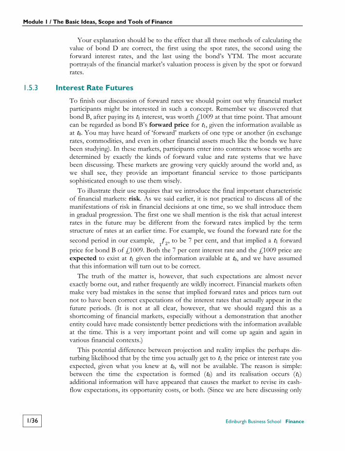
Module 1 / The Basic Ideas, Scope and Tools of Finance
1/36 Edinburgh Business School Finance
Your explanation should be to the effect that all three methods of calculating the value of bond D are correct, the first using the spot rates, the second using the forward interest rates, and the last using the bond’s YTM. The most accurate portrayals of the financial market’s valuation process is given by the spot or forward rates.
1.5.3 Interest Rate Futures
To finish our discussion of forward rates we should point out why financial market participants might be interested in such a concept. Remember we discovered that bond B, after paying its t1 interest, was worth £1009 at that time point. That amount can be regarded as bond B’s forward price for t1, given the information available as at t0. You may have heard of ‘forward’ markets of one type or another (in exchange rates, commodities, and even in other financial assets much like the bonds we have been studying). In these markets, participants enter into contracts whose worths are determined by exactly the kinds of forward value and rate systems that we have been discussing. These markets are growing very quickly around the world and, as we shall see, they provide an important financial service to those participants sophisticated enough to use them wisely.
To illustrate their use requires that we introduce the final important characteristic of financial markets: risk. As we said earlier, it is not practical to discuss all of the manifestations of risk in financial decisions at one time, so we shall introduce them in gradual progression. The first one we shall mention is the risk that actual interest rates in the future may be different from the forward rates implied by the term structure of rates at an earlier time. For example, we found the forward rate for the second period in our example, 21 , to be 7 per cent, and that implied a t1 forward price for bond B of £1009. Both the 7 per cent interest rate and the £1009 price are expected to exist at t1 given the information available at t0, and we have assumed that this information will turn out to be correct.
The truth of the matter is, however, that such expectations are almost never exactly borne out, and rather frequently are wildly incorrect. Financial markets often make very bad mistakes in the sense that implied forward rates and prices turn out not to have been correct expectations of the interest rates that actually appear in the future periods. (It is not at all clear, however, that we should regard this as a shortcoming of financial markets, especially without a demonstration that another entity could have made consistently better predictions with the information available at the time. This is a very important point and will come up again and again in various financial contexts.)
This potential difference between projection and reality implies the perhaps dis-turbing likelihood that by the time you actually get to t1 the price or interest rate you expected, given what you knew at t0, will not be available. The reason is simple: between the time the expectation is formed (t0) and its realisation occurs (t1) additional information will have appeared that causes the market to revise its cash-flow expectations, its opportunity costs, or both. (Since we are here discussing only
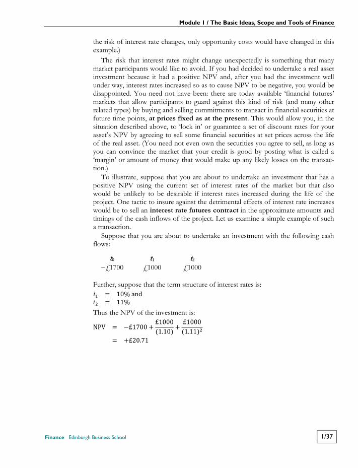
Module 1 / The Basic Ideas, Scope and Tools of Finance
Finance Edinburgh Business School 1/37
the risk of interest rate changes, only opportunity costs would have changed in this example.)
The risk that interest rates might change unexpectedly is something that many market participants would like to avoid. If you had decided to undertake a real asset investment because it had a positive NPV and, after you had the investment well under way, interest rates increased so as to cause NPV to be negative, you would be disappointed. You need not have been: there are today available ‘financial futures’ markets that allow participants to guard against this kind of risk (and many other related types) by buying and selling commitments to transact in financial securities at future time points, at prices fixed as at the present. This would allow you, in the situation described above, to ‘lock in’ or guarantee a set of discount rates for your asset’s NPV by agreeing to sell some financial securities at set prices across the life of the real asset. (You need not even own the securities you agree to sell, as long as you can convince the market that your credit is good by posting what is called a ‘margin’ or amount of money that would make up any likely losses on the transac-tion.)
To illustrate, suppose that you are about to undertake an investment that has a positive NPV using the current set of interest rates of the market but that also would be unlikely to be desirable if interest rates increased during the life of the project. One tactic to insure against the detrimental effects of interest rate increases would be to sell an interest rate futures contract in the approximate amounts and timings of the cash inflows of the project. Let us examine a simple example of such a transaction.
Suppose that you are about to undertake an investment with the following cash flows: t0 t1 t2 −£1700 £1000 £1000
Further, suppose that the term structure of interest rates is: = 10% and= 11% Thus the NPV of the investment is: NPV = −£1700 + £1000(1.10) + £1000(1.11)= +£20.71
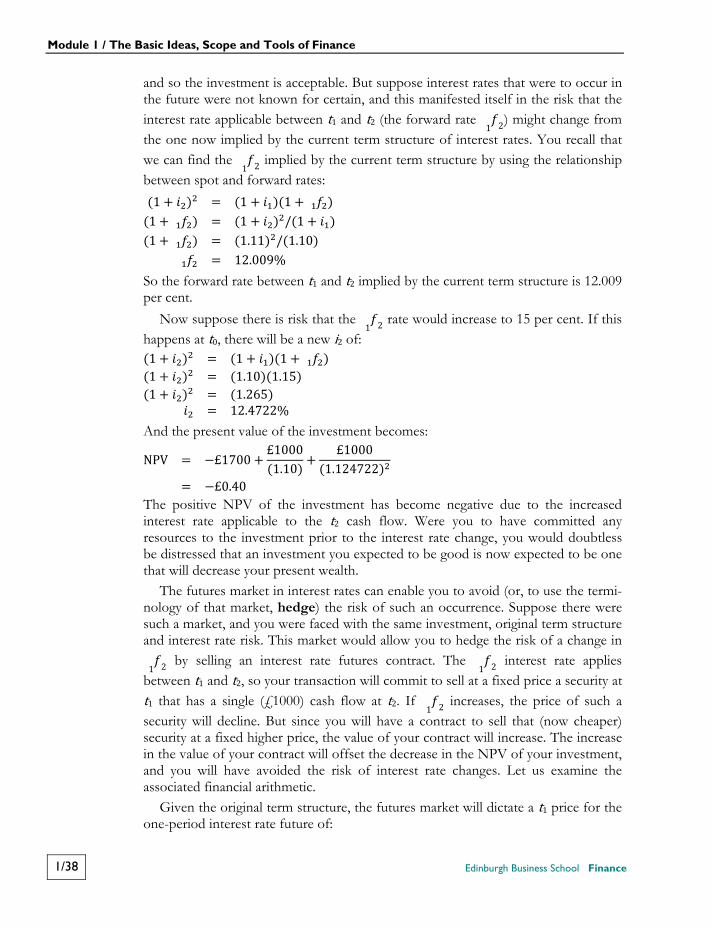
Module 1 / The Basic Ideas, Scope and Tools of Finance
1/38 Edinburgh Business School Finance
and so the investment is acceptable. But suppose interest rates that were to occur in the future were not known for certain, and this manifested itself in the risk that the interest rate applicable between t1 and t2 (the forward rate 21 ) might change from the one now implied by the current term structure of interest rates. You recall that we can find the 21 implied by the current term structure by using the relationship between spot and forward rates: (1 + ) = (1 + )(1 + )(1 + ) = (1 + ) /(1 + )(1 + ) = (1.11) /(1.10)= 12.009% So the forward rate between t1 and t2 implied by the current term structure is 12.009 per cent.
Now suppose there is risk that the 21 rate would increase to 15 per cent. If this happens at t0, there will be a new i2 of: (1 + ) = (1 + )(1 + )(1 + ) = (1.10)(1.15)(1 + ) = (1.265)= 12.4722% And the present value of the investment becomes: NPV = −£1700 + £1000(1.10) + £1000(1.124722)= −£0.40 The positive NPV of the investment has become negative due to the increased interest rate applicable to the t2 cash flow. Were you to have committed any resources to the investment prior to the interest rate change, you would doubtless be distressed that an investment you expected to be good is now expected to be one that will decrease your present wealth.
The futures market in interest rates can enable you to avoid (or, to use the termi-nology of that market, hedge) the risk of such an occurrence. Suppose there were such a market, and you were faced with the same investment, original term structure and interest rate risk. This market would allow you to hedge the risk of a change in 21 by selling an interest rate futures contract. The 21 interest rate applies between t1 and t2, so your transaction will commit to sell at a fixed price a security at t1 that has a single (£1000) cash flow at t2. If 21 increases, the price of such a security will decline. But since you will have a contract to sell that (now cheaper) security at a fixed higher price, the value of your contract will increase. The increase in the value of your contract will offset the decrease in the NPV of your investment, and you will have avoided the risk of interest rate changes. Let us examine the associated financial arithmetic.
Given the original term structure, the futures market will dictate a t1 price for the one-period interest rate future of:
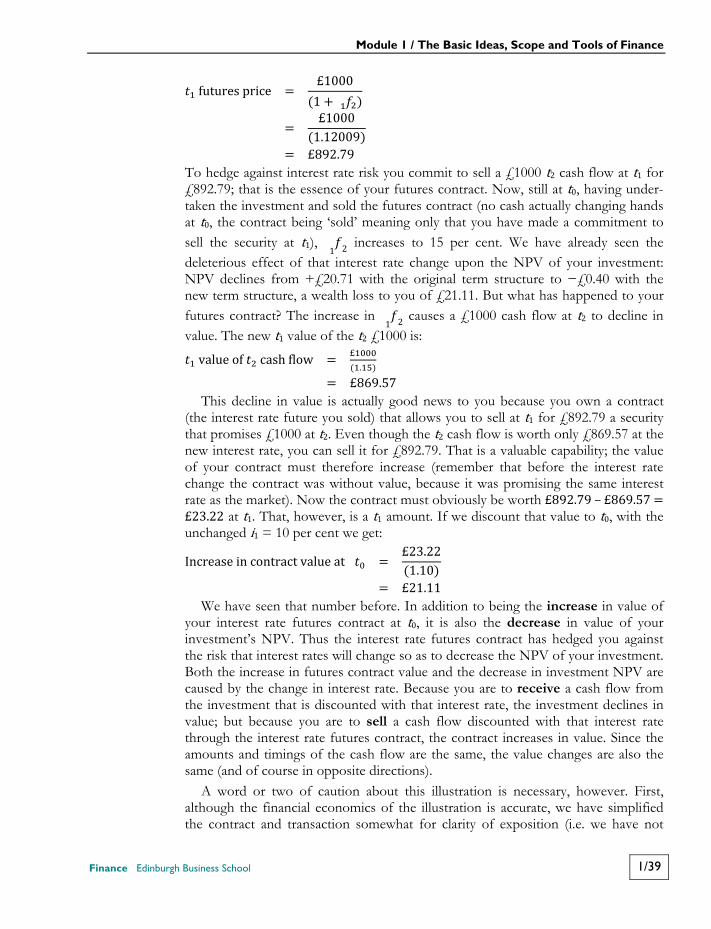
Module 1 / The Basic Ideas, Scope and Tools of Finance
Finance Edinburgh Business School 1/39
futures price = £1000(1 + )= £1000(1.12009)= £892.79
To hedge against interest rate risk you commit to sell a £1000 t2 cash flow at t1 for £892.79; that is the essence of your futures contract. Now, still at t0, having under-taken the investment and sold the futures contract (no cash actually changing hands at t0, the contract being ‘sold’ meaning only that you have made a commitment to sell the security at t1), 21 increases to 15 per cent. We have already seen the deleterious effect of that interest rate change upon the NPV of your investment: NPV declines from +£20.71 with the original term structure to −£0.40 with the new term structure, a wealth loss to you of £21.11. But what has happened to your futures contract? The increase in 21 causes a £1000 cash flow at t2 to decline in value. The new t1 value of the t2 £1000 is: value of cash flow = £( . )= £869.57
This decline in value is actually good news to you because you own a contract (the interest rate future you sold) that allows you to sell at t1 for £892.79 a security that promises £1000 at t2. Even though the t2 cash flow is worth only £869.57 at the new interest rate, you can sell it for £892.79. That is a valuable capability; the value of your contract must therefore increase (remember that before the interest rate change the contract was without value, because it was promising the same interest rate as the market). Now the contract must obviously be worth £892.79 – £869.57 = £23.22 at t1. That, however, is a t1 amount. If we discount that value to t0, with the unchanged i1 = 10 per cent we get: Increase in contract value at = £23.22(1.10)= £21.11
We have seen that number before. In addition to being the increase in value of your interest rate futures contract at t0, it is also the decrease in value of your investment’s NPV. Thus the interest rate futures contract has hedged you against the risk that interest rates will change so as to decrease the NPV of your investment. Both the increase in futures contract value and the decrease in investment NPV are caused by the change in interest rate. Because you are to receive a cash flow from the investment that is discounted with that interest rate, the investment declines in value; but because you are to sell a cash flow discounted with that interest rate through the interest rate futures contract, the contract increases in value. Since the amounts and timings of the cash flow are the same, the value changes are also the same (and of course in opposite directions).
A word or two of caution about this illustration is necessary, however. First, although the financial economics of the illustration is accurate, we have simplified the contract and transaction somewhat for clarity of exposition (i.e. we have not
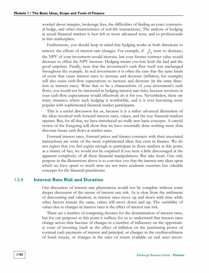
Module 1 / The Basic Ideas, Scope and Tools of Finance
1/40 Edinburgh Business School Finance
worried about margins, brokerage fees, the difficulties of finding an exact contractu-al hedge, and other characteristics of real-life transactions). The analysis of hedging in actual financial markets is best left to more advanced texts, and to professionals in that marketplace.
Furthermore, you should keep in mind that hedging works in both directions to remove the effects of interest rate changes. For example, if 21 were to decrease, the NPV of your investment would increase, but your futures contract value would decrease to offset the NPV increase. Hedging means you lose both the bad and the good surprises. Finally, note that the investment’s cash flow itself was unchanged throughout the example. In real investments it is often the case that the same kinds of event that cause interest rates to increase and decrease (inflation, for example) will also cause cash-flow expectations to increase and decrease (in the same direc-tion as interest rates). Were that to be a characteristic of your investment’s cash flows, you would not be interested in hedging interest rate risks, because revisions in your cash-flow expectations would effectively do it for you. Nevertheless, there are many instances where such hedging is worthwhile, and it is ever becoming more popular with sophisticated financial market participants.
This is a useful discussion for us, because it is a rather advanced illustration of the ideas involved with forward interest rates, values, and the way financial markets operate. But, for all that, we have introduced no really new basic concepts. A careful review of the foregoing will show that we have essentially done nothing more than discount future cash flows at market rates.
Forward interest rates, forward prices and futures contracts with their associated transactions are some of the more sophisticated ideas that exist in finance. We do not expect that you feel expert enough to participate in those markets at this point; as a matter of fact, we would not be surprised if you were a little discouraged at the apparent complexity of all these financial manipulations. But take heart. Our only purpose in the illustrations above is to convince you that the interest rate ideas upon which we have spent so much time are not mere academic exercises but valuable concepts for the financial practitioner.
1.5.4 Interest Rate Risk and Duration
Our discussion of interest rate phenomena would not be complete without some deeper discussion of the nature of interest rate risk. As is clear from the arithmetic of discounting and valuation, as interest rates move up and down with time while other factors remain the same, values will move down and up. The variability of values due to changes in interest rates is the effect of interest rate risk.
There are a number of competing theories for the determination of interest rates, but for our purposes at this point it suffices for us to understand that interest rates change across time because of changes in a number of influences on the opportuni-ty costs of investing (such as the effect of inflation on the purchasing power of eventual cash payments of interest and principal, or changes in the creditworthiness of bond issuers, or changes in the rates of return available on real asset invest-
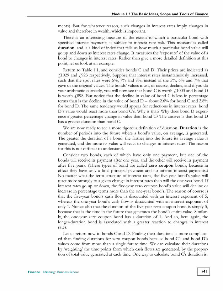
Module 1 / The Basic Ideas, Scope and Tools of Finance
Finance Edinburgh Business School 1/41
ments). But for whatever reason, such changes in interest rates imply changes in value and therefore in wealth, which is important.
There is an interesting measure of the extent to which a particular bond with specified interest payments is subject to interest rate risk. This measure is called duration, and is a kind of index that tells us how much a particular bond value will go up and down as interest rates change. It measures the ‘exposure’ of the value of a bond to changes in interest rates. Rather than give a more detailed definition at this point, let us look at an example.
Return to Table 1.1, and consider bonds C and D. Their prices are indicated as £1029 and £923 respectively. Suppose that interest rates instantaneously increased, such that the spot rates were 6%, 7% and 8%, instead of the 5%, 6% and 7% that gave us the original values. The bonds’ values must, of course, decline, and if you do your arithmetic correctly, you will now see that bond C is worth £1003 and bond D is worth £898. But notice that the decline in value of bond C is less in percentage terms than is the decline in the value of bond D – about 2.6% for bond C and 2.8% for bond D. The same tendency would appear for reductions in interest rates: bond D’s value would react more than bond C’s. Why is that? Why does bond D experi-ence a greater percentage change in value than bond C? The answer is that bond D has a greater duration than bond C.
We are now ready to see a more rigorous definition of duration. Duration is the number of periods into the future where a bond’s value, on average, is generated. The greater the duration of a bond, the farther into the future its average value is generated, and the more its value will react to changes in interest rates. The reason for this is not difficult to understand.
Consider two bonds, each of which have only one payment, but one of the bonds will receive its payment after one year, and the other will receive its payment after five years. (These types of bond are called zero coupon bonds, because in effect they have only a final principal payment and no interim interest payments.) No matter what the term structure of interest rates, the five-year bond’s value will react more strongly to a given change in interest rates than will the one-year bond. If interest rates go up or down, the five-year zero coupon bond’s value will decline or increase in percentage terms more than the one-year bond’s. The reason of course is that the five-year bond’s cash flow is discounted with an interest exponent of 5, whereas the one-year bond’s cash flow is discounted with an interest exponent of only 1. Notice also that the duration of the five-year zero coupon bond is simply 5, because that is the time in the future that generates the bond’s entire value. Similar-ly, the one-year zero coupon bond has a duration of 1. And so, here again, the longer-duration bond is associated with a greater reaction to changes in interest rates.
Let us return now to bonds C and D. Finding their durations is more complicat-ed than finding durations for zero coupon bonds because bond C’s and bond D’s values come from more than a single future time. We can calculate their durations by ‘weighting’ the time points from which cash flows are generated, by the propor-tion of total value generated at each time. One way to calculate bond C’s duration is:
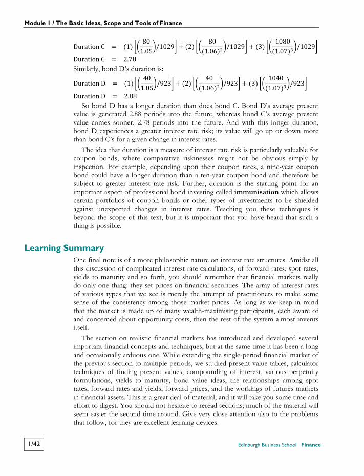
Module 1 / The Basic Ideas, Scope and Tools of Finance
1/42 Edinburgh Business School Finance
Duration C = (1) 801.05 /1029 + (2) 80(1.06) /1029 + (3) 1080(1.07) /1029Duration C = 2.78 Similarly, bond D’s duration is: Duration D = (1) 401.05 /923 + (2) 40(1.06) /923 + (3) 1040(1.07) /923Duration D = 2.88
So bond D has a longer duration than does bond C. Bond D’s average present value is generated 2.88 periods into the future, whereas bond C’s average present value comes sooner, 2.78 periods into the future. And with this longer duration, bond D experiences a greater interest rate risk; its value will go up or down more than bond C’s for a given change in interest rates.
The idea that duration is a measure of interest rate risk is particularly valuable for coupon bonds, where comparative riskinesses might not be obvious simply by inspection. For example, depending upon their coupon rates, a nine-year coupon bond could have a longer duration than a ten-year coupon bond and therefore be subject to greater interest rate risk. Further, duration is the starting point for an important aspect of professional bond investing called immunisation which allows certain portfolios of coupon bonds or other types of investments to be shielded against unexpected changes in interest rates. Teaching you these techniques is beyond the scope of this text, but it is important that you have heard that such a thing is possible.
Learning Summary One final note is of a more philosophic nature on interest rate structures. Amidst all this discussion of complicated interest rate calculations, of forward rates, spot rates, yields to maturity and so forth, you should remember that financial markets really do only one thing: they set prices on financial securities. The array of interest rates of various types that we see is merely the attempt of practitioners to make some sense of the consistency among those market prices. As long as we keep in mind that the market is made up of many wealth-maximising participants, each aware of and concerned about opportunity costs, then the rest of the system almost invents itself.
The section on realistic financial markets has introduced and developed several important financial concepts and techniques, but at the same time it has been a long and occasionally arduous one. While extending the single-period financial market of the previous section to multiple periods, we studied present value tables, calculator techniques of finding present values, compounding of interest, various perpetuity formulations, yields to maturity, bond value ideas, the relationships among spot rates, forward rates and yields, forward prices, and the workings of futures markets in financial assets. This is a great deal of material, and it will take you some time and effort to digest. You should not hesitate to reread sections; much of the material will seem easier the second time around. Give very close attention also to the problems that follow, for they are excellent learning devices.
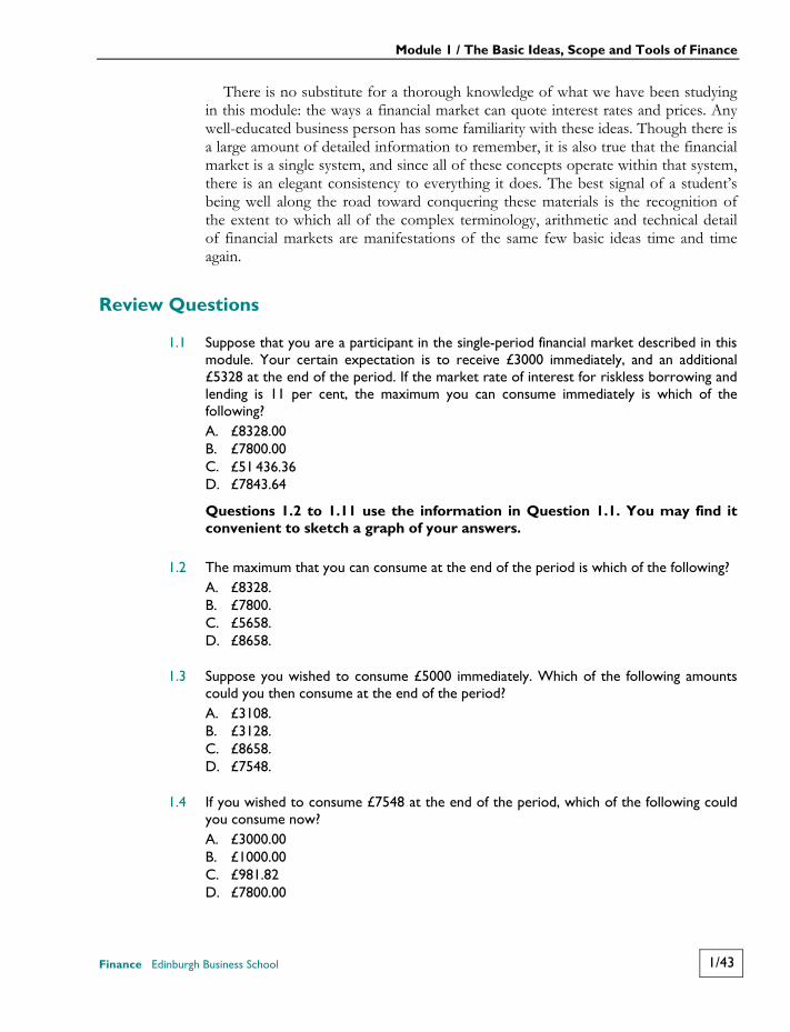
Module 1 / The Basic Ideas, Scope and Tools of Finance
Finance Edinburgh Business School 1/43
There is no substitute for a thorough knowledge of what we have been studying in this module: the ways a financial market can quote interest rates and prices. Any well-educated business person has some familiarity with these ideas. Though there is a large amount of detailed information to remember, it is also true that the financial market is a single system, and since all of these concepts operate within that system, there is an elegant consistency to everything it does. The best signal of a student’s being well along the road toward conquering these materials is the recognition of the extent to which all of the complex terminology, arithmetic and technical detail of financial markets are manifestations of the same few basic ideas time and time again.
Review Questions
1.1 Suppose that you are a participant in the single-period financial market described in this module. Your certain expectation is to receive £3000 immediately, and an additional £5328 at the end of the period. If the market rate of interest for riskless borrowing and lending is 11 per cent, the maximum you can consume immediately is which of the following? A. £8328.00 B. £7800.00 C. £51 436.36 D. £7843.64
Questions 1.2 to 1.11 use the information in Question 1.1. You may find itconvenient to sketch a graph of your answers.
1.2 The maximum that you can consume at the end of the period is which of the following? A. £8328. B. £7800. C. £5658. D. £8658.
1.3 Suppose you wished to consume £5000 immediately. Which of the following amounts could you then consume at the end of the period? A. £3108. B. £3128. C. £8658. D. £7548.
1.4 If you wished to consume £7548 at the end of the period, which of the following could you consume now? A. £3000.00 B. £1000.00 C. £981.82 D. £7800.00
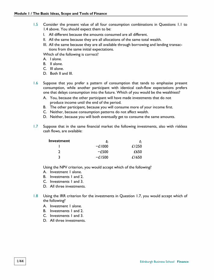
Module 1 / The Basic Ideas, Scope and Tools of Finance
1/44 Edinburgh Business School Finance
1.5 Consider the present value of all four consumption combinations in Questions 1.1 to 1.4 above. You should expect them to be: I. All different because the amounts consumed are all different. II. All the same because they are all allocations of the same total wealth. III. All the same because they are all available through borrowing and lending transac-
tions from the same initial expectations. Which of the following is correct? A. I alone. B. II alone. C. III alone. D. Both II and III.
1.6 Suppose that you prefer a pattern of consumption that tends to emphasise present consumption, while another participant with identical cash-flow expectations prefers one that delays consumption into the future. Which of you would be the wealthiest? A. You, because the other participant will have made investments that do not
produce income until the end of the period.
B. The other participant, because you will consume more of your income first. C. Neither, because consumption patterns do not affect wealth. D. Neither, because you will both eventually get to consume the same amounts.
1.7 Suppose that in the same financial market the following investments, also with riskless cash flows, are available:
Investment t0 t11 −£1000 £12502 −£500 £6503 −£1500 £1650
Using the NPV criterion, you would accept which of the following? A. Investment 1 alone. B. Investments 1 and 2. C. Investments 1 and 3. D. All three investments.
1.8 Using the IRR criterion for the investments in Question 1.7, you would accept which of the following? A. Investment 1 alone. B. Investments 1 and 2. C. Investments 1 and 3. D. All three investments.
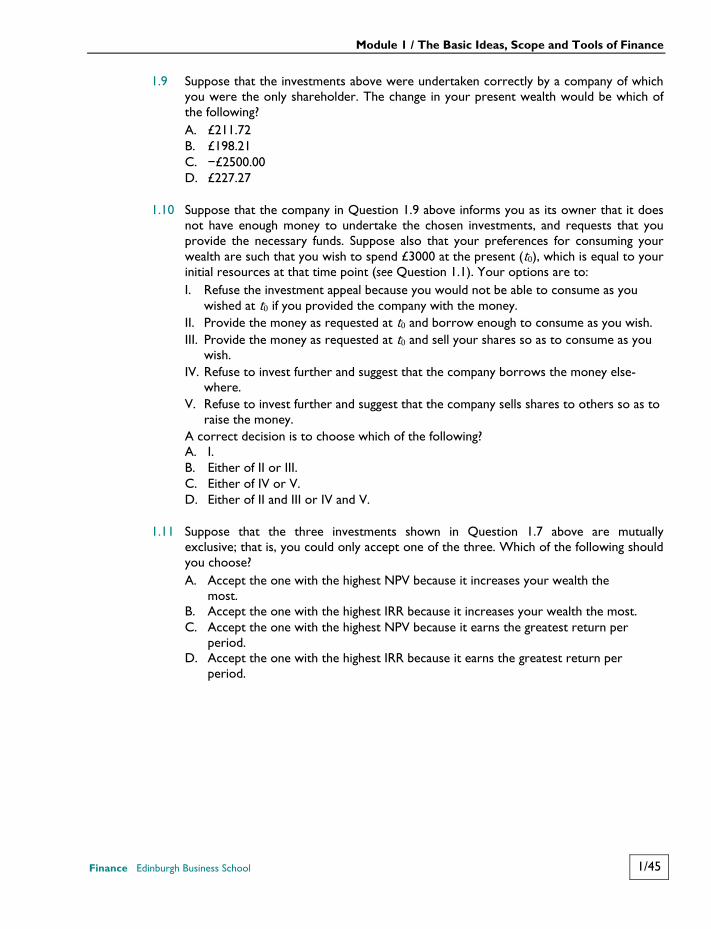
Module 1 / The Basic Ideas, Scope and Tools of Finance
Finance Edinburgh Business School 1/45
1.9 Suppose that the investments above were undertaken correctly by a company of which you were the only shareholder. The change in your present wealth would be which of the following? A. £211.72 B. £198.21 C. −£2500.00 D. £227.27
1.10 Suppose that the company in Question 1.9 above informs you as its owner that it does not have enough money to undertake the chosen investments, and requests that you provide the necessary funds. Suppose also that your preferences for consuming your wealth are such that you wish to spend £3000 at the present (t0), which is equal to your initial resources at that time point (see Question 1.1). Your options are to: I. Refuse the investment appeal because you would not be able to consume as you
wished at t0 if you provided the company with the money. II. Provide the money as requested at t0 and borrow enough to consume as you wish. III. Provide the money as requested at t0 and sell your shares so as to consume as you
wish. IV. Refuse to invest further and suggest that the company borrows the money else-
where. V. Refuse to invest further and suggest that the company sells shares to others so as to
raise the money. A correct decision is to choose which of the following? A. I. B. Either of II or III. C. Either of IV or V. D. Either of II and III or IV and V.
1.11 Suppose that the three investments shown in Question 1.7 above are mutually exclusive; that is, you could only accept one of the three. Which of the following should you choose? A. Accept the one with the highest NPV because it increases your wealth the
most.
B. Accept the one with the highest IRR because it increases your wealth the most. C. Accept the one with the highest NPV because it earns the greatest return per
period.
D. Accept the one with the highest IRR because it earns the greatest return per period.
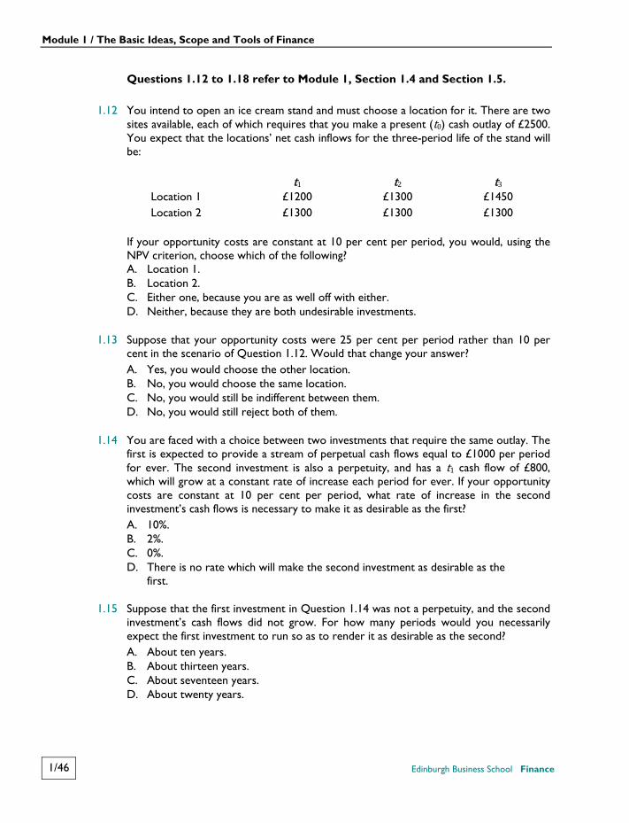
Module 1 / The Basic Ideas, Scope and Tools of Finance
1/46 Edinburgh Business School Finance
Questions 1.12 to 1.18 refer to Module 1, Section 1.4 and Section 1.5.
1.12 You intend to open an ice cream stand and must choose a location for it. There are two sites available, each of which requires that you make a present (t0) cash outlay of £2500. You expect that the locations’ net cash inflows for the three-period life of the stand will be:
t1 t2 t3 Location 1 £1200 £1300 £1450 Location 2 £1300 £1300 £1300
If your opportunity costs are constant at 10 per cent per period, you would, using the NPV criterion, choose which of the following? A. Location 1. B. Location 2. C. Either one, because you are as well off with either. D. Neither, because they are both undesirable investments.
1.13 Suppose that your opportunity costs were 25 per cent per period rather than 10 per cent in the scenario of Question 1.12. Would that change your answer? A. Yes, you would choose the other location. B. No, you would choose the same location. C. No, you would still be indifferent between them. D. No, you would still reject both of them.
1.14 You are faced with a choice between two investments that require the same outlay. The first is expected to provide a stream of perpetual cash flows equal to £1000 per period for ever. The second investment is also a perpetuity, and has a t1 cash flow of £800, which will grow at a constant rate of increase each period for ever. If your opportunity costs are constant at 10 per cent per period, what rate of increase in the second investment’s cash flows is necessary to make it as desirable as the first? A. 10%. B. 2%. C. 0%. D. There is no rate which will make the second investment as desirable as the
first.
1.15 Suppose that the first investment in Question 1.14 was not a perpetuity, and the second investment’s cash flows did not grow. For how many periods would you necessarily expect the first investment to run so as to render it as desirable as the second? A. About ten years. B. About thirteen years. C. About seventeen years. D. About twenty years.
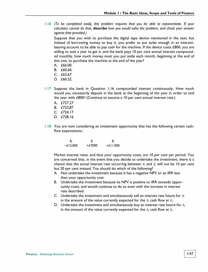
Module 1 / The Basic Ideas, Scope and Tools of Finance
Finance Edinburgh Business School 1/47
1.16 (To be completed easily, this problem requires that you be able to exponentiate. If your calculator cannot do that, describe how you would solve the problem, and check your answer against that provided.) Suppose that you wish to purchase the digital tape device mentioned in the text, but instead of borrowing money to buy it, you prefer to put aside enough in an interest-bearing account to be able to pay cash for the machine. If the device costs £800, you are willing to wait a year to get it, and the bank pays 10 per cent annual interest compound-ed monthly, how much money must you put aside each month, beginning at the end of this one, to purchase the machine at the end of the year? A. £66.00. B. £60.60. C. £63.67. D. £60.32.
1.17 Suppose the bank in Question 1.16 compounded interest continuously. How much would you necessarily deposit in the bank at the beginning of the year in order to end the year with £800? (Continue to assume a 10 per cent annual interest rate.) A. £727.27 B. £723.87 C. £724.17 D. £738.16
1.18 You are now considering an investment opportunity that has the following certain cash-flow expectations: t0 t1 t2
−£15 000 +£7000 +£11 000
Market interest rates, and thus your opportunity costs, are 10 per cent per period. You are concerned that, in the event that you decide to undertake the investment, there is a chance that the actual interest rate occurring between t1 and t2 will not be 10 per cent but 20 per cent instead. You should do which of the following? A. Not undertake the investment because it has a negative NPV or an IRR less
than your opportunity cost.
B. Undertake the investment because its NPV is positive or IRR exceeds oppor-tunity costs, and would continue to do so even with the increase in interest rate described.
C. Undertake the investment and simultaneously sell an interest rate future for t1 in the amount of the value currently expected for the t2 cash flow at t1.
D. Undertake the investment and simultaneously buy an interest rate future for t1 in the amount of the value currently expected for the t2 cash flow at t1.
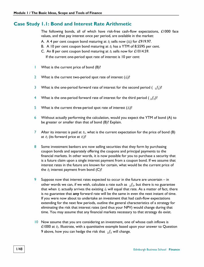
Module 1 / The Basic Ideas, Scope and Tools of Finance
1/48 Edinburgh Business School Finance
Case Study 1.1: Bond and Interest Rate Arithmetic The following bonds, all of which have risk-free cash-flow expectations, £1000 face values, and that pay interest once per period, are available in the market:
A. A 4 per cent coupon bond maturing at t2 sells now (t0) for £919.97. B. A 10 per cent coupon bond maturing at t2 has a YTM of 8.5595 per cent. C. An 8 per cent coupon bond maturing at t3 sells now for £1014.59.
If the current one-period spot rate of interest is 10 per cent:
1 What is the current price of bond (B)?
2 What is the current two-period spot rate of interest (i2)? 3 What is the one-period forward rate of interest for the second period ( )?
4 What is the one-period forward rate of interest for the third period ( )?
5 What is the current three-period spot rate of interest (i3)? 6 Without actually performing the calculation, would you expect the YTM of bond (A) to
be greater or smaller than that of bond (B)? Explain.
7 After its interest is paid at t1, what is the current expectation for the price of bond (B) at t1 (its forward price at t1)?
8 Some investment bankers are now selling securities that they form by purchasing coupon bonds and separately offering the coupons and principal payments to the financial markets. In other words, it is now possible for you to purchase a security that is a future claim upon a single interest payment from a coupon bond. If we assume that interest rates in the future are known for certain, what would be the current price of the t2 interest payment from bond (C)?
9 Suppose now that interest rates expected to occur in the future are uncertain – in other words we can, if we wish, calculate a rate such as , but there is no guarantee that when t2 actually arrives the existing i2 will equal that rate. As a matter of fact, there is no guarantee that any forward rate will be the same in even the next instant of time. If you were now about to undertake an investment that had cash-flow expectations extending for the next few periods, outline the general characteristics of a strategy for eliminating the risk that interest rates (and thus your NPV) would change during that time. You may assume that any financial markets necessary to that strategy do exist.
10 Now assume that you are considering an investment, one of whose cash inflows is £1000 at t3. Illustrate, with a quantitative example based upon your answer to Question 9 above, how you can hedge the risk that will change.
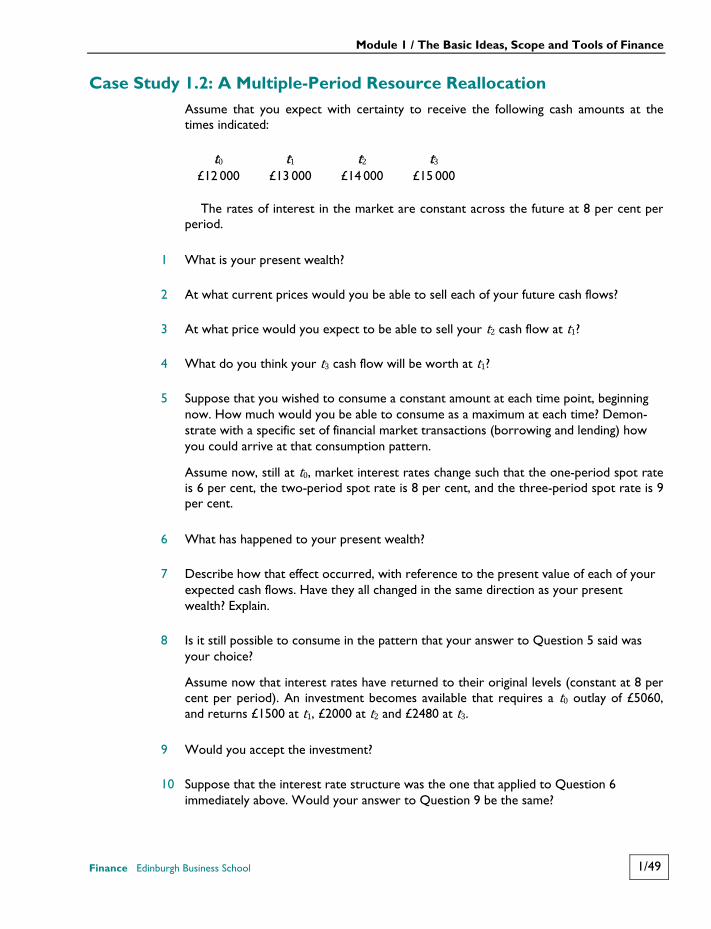
Module 1 / The Basic Ideas, Scope and Tools of Finance
Finance Edinburgh Business School 1/49
Case Study 1.2: A Multiple-Period Resource Reallocation Assume that you expect with certainty to receive the following cash amounts at thetimes indicated: t0 t1 t2 t3
£12 000 £13 000 £14 000 £15 000
The rates of interest in the market are constant across the future at 8 per cent perperiod.
1 What is your present wealth?
2 At what current prices would you be able to sell each of your future cash flows?
3 At what price would you expect to be able to sell your t2 cash flow at t1? 4 What do you think your t3 cash flow will be worth at t1? 5 Suppose that you wished to consume a constant amount at each time point, beginning
now. How much would you be able to consume as a maximum at each time? Demon-strate with a specific set of financial market transactions (borrowing and lending) how you could arrive at that consumption pattern.
Assume now, still at t0, market interest rates change such that the one-period spot rate is 6 per cent, the two-period spot rate is 8 per cent, and the three-period spot rate is 9 per cent.
6 What has happened to your present wealth?
7 Describe how that effect occurred, with reference to the present value of each of your expected cash flows. Have they all changed in the same direction as your present wealth? Explain.
8 Is it still possible to consume in the pattern that your answer to Question 5 said was your choice?
Assume now that interest rates have returned to their original levels (constant at 8 percent per period). An investment becomes available that requires a t0 outlay of £5060, and returns £1500 at t1, £2000 at t2 and £2480 at t3.
9 Would you accept the investment?
10 Suppose that the interest rate structure was the one that applied to Question 6 immediately above. Would your answer to Question 9 be the same?

Module 1 / The Basic Ideas, Scope and Tools of Finance
1/50 Edinburgh Business School Finance
11 Suppose that the cash flows for the investment at t1 and t3 were swapped. Would the relative desirability of the investment with the two interest rate structures be the same? Explain.