Finance and Economics Discussion SeriesDivisions of Research & Statistics and Monetary Affairs

Federal Reserve Board, Washington, D.C.

Systemic Risk Contributions

Xin Huang, Hao Zhou, and Haibin Zhu

2011-08

NOTE: Staff working papers in the Finance and Economics Discussion Series (FEDS) are preliminarymaterials circulated to stimulate discussion and critical comment. The analysis and conclusions set forthare those of the authors and do not indicate concurrence by other members of the research staff or theBoard of Governors. References in publications to the Finance and Economics Discussion Series (other thanacknowledgement) should be cleared with the author(s) to protect the tentative character of these papers.

Systemic Risk Contributions∗

Xin Huang†

Hao Zhou‡

Haibin Zhu§

First Draft: August 2010This Version: January 2011

Abstract

We adopt a systemic risk indicator measured by the price of insurance againstsystemic financial distress and assess individual banks’ marginal contributions to thesystemic risk. The methodology is applied using publicly available data to the 19bank holding companies covered by the U.S. Supervisory Capital Assessment Program(SCAP), with the systemic risk indicator peaking around $1.1 trillion in March 2009.Our systemic risk contribution measure shows interesting similarity to and divergencefrom the SCAP expected loss measure. In general, we find that a bank’s contributionto the systemic risk is roughly linear in its default probability but highly nonlinearwith respect to institution size and asset correlation.

JEL classification: G21, G28, G14.Keywords: Distress Insurance Premium, Systemic Risk, Macroprudential Regulation, LargeComplex Financial Institution, Too-Big-to-Fail, Too-Connected-to-Fail.

∗We would like to thank Viral Acharya, Tobias Adrian, Sean Campbell, Myron Kwast, Frank Packer,Nikola Tarashev, James Wilcox, Robert DeYoung, and seminar participants at the Federal Reserve, ChicagoBank Structure Conference, IMF Conference on Operationalizing Systemic Risk Monitoring, Fields InstituteFinancial Stability Forum, NUS Risk Management Conference, Bank of England and CAREFIN (Centre forApplied Research in Finance, University of Bocconi) Conference on Matching Stability and Performance,and Bank Research Conference at FDIC for their helpful commments. James Marrone provided excellentresearch assistance. We also thank Christopher Karlsten for editing assistance. The views presented hereare solely those of the authors and do not necessarily represent those of the Federal Reserve Board or theBank for International Settlements.

†Department of Economics, University of Oklahoma, Norman, Oklahoma, USA; phone: 1-405-325-2643;e-mail: xhuang@ou.edu.

‡Corresponding Author: Risk Analysis Section, Federal Reserve Board, Washington, D.C., USA;phone: 1-202-452-3360; e-mail: hao.zhou@frb.gov.

§Bank for International Settlements, Representative Office for Asia and the Pacific, Hong Kong; phone:852-2878-7145; e-mail: haibin.zhu@bis.org.

Systemic Risk Contributions

Abstract

We adopt a systemic risk indicator measured by the price of insurance against systemic

financial distress and assess individual banks’ marginal contributions to the systemic risk.

The methodology is applied using publicly available data to the 19 bank holding companies

covered by the U.S. Supervisory Capital Assessment Program (SCAP), with the systemic

risk indicator peaking around $1.1 trillion in March 2009. Our systemic risk contribution

measure shows interesting similarity to and divergence from the SCAP expected loss measure.

In general, we find that a bank’s contribution to the systemic risk is roughly linear in its

default probability but highly nonlinear with respect to institution size and asset correlation.

JEL classification: G21, G28, G14.

Keywords: Distress Insurance Premium, Systemic Risk, Macroprudential Regulation, Large

Complex Financial Institution, Too-Big-to-Fail, Too-Connected-to-Fail.

1 Introduction

The recent global financial crisis has led bank supervisors and regulators to rethink the

rationale of banking regulation. One important lesson is that the traditional approach to

ensuring the soundness of individual banks, as in Basel I and Basel II, needs to be supple-

mented by a system-wide macroprudential approach. The macroprudential perspective of

supervision focuses on the soundness of the banking system as a whole and the inter-linkages

among those systemically important banks. This perspective has become an overwhelming

theme in the policy deliberations among legislative committees, bank regulators, and aca-

demic researchers.1 As stated in the Financial Stability Board’s interim report in June 2010,

“Financial institutions should be subject to requirements commensurate with the risks they

pose to the financial system.”

However, implementing such a macroprudential perspective is not an easy task. The

operational framework needs to provide answers to three crucial questions. First, how should

the systemic risk in a financial system be measured? Second, how should the contributions

of individual banks (or financial institutions) to the systemic risk be measured? Third, how

can prudential requirements on individual banks, such as capital surcharges, taxes, or fees

for a financial stability fund, be designed so that they are connected with banks’ systemic

risk contributions?

Against such a background, this paper proposes a consistent framework that provides

direct answers to the first two questions, the results of which can be used as helpful inputs to

address the third question. Our systemic risk measure can be interpreted economically as the

insurance premium to cover distressed losses in a banking system, which is a concept of a risk-

neutral market price, assuming that such an insurance market exists and functions properly

(Huang, Zhou, and Zhu, 2009). Within the same framework, the systemic importance of

each bank (or bank group) can be properly defined as its marginal contribution to the

hypothetical distress insurance premium (DIP) of the whole banking system. This approach

1See, for instance, Brunnermeier et al. (2009), Financial Stability Forum (2009a,b), Panetta et al. (2009),and BCBS (2009), among others. The macroprudential perspective was proposed by Crocket (2000), Borio(2003), and Acharya (2009).

1

allows us to study the time variation and cross section of the systemic risk contributions

of U.S. large complex financial institutions (LCFIs). Our metric can be applied using only

publicly available information for large banking organizations.

Adopting such a consistent approach has advantages. Under such a framework, the

marginal contribution of each bank adds up to the aggregate systemic risk. As shown

in Tarashev, Borio, and Tsatsaronis (2009a), this additivity property is desirable from an

operational perspective because it allows the macroprudential tools to be implemented at

individual bank levels. In particular, prudential requirements can be linear transformations

of the marginal contribution measures if the measures are additive. One can also decompose

our systemic risk measures into different economic channels—for example, risk premium

versus actual default risk and credit risk versus liquidity risk. Finally, since our structural

framework uses default probabilities, liability sizes, and correlations directly as inputs to

capture the well publicized characteristics of systemic risk—leverage, too-big-to-fail, and too-

connected-to-fail—one can easily swap these inputs with supervisory confidential information

for practical policy analysis.

We applied this approach to the 19 bank holding companies (BHCs) covered by the U.S.

Supervisory Capital Assessment Program (SCAP)—commonly known as the “stress test”—

during the period from January 2004 to December 2009. However, unlike the SCAP, our

analysis did not rely on any confidential, supervisory, or proprietary information or data.

Our findings suggest that the systemic risk indicator stood at its peak around $1.1 trillion in

March 2009 and has since fallen to about $300 billion—the level reached in January 2008. A

bank’s contribution to the systemic risk indicator appears to be linearly related to its default

probability but highly nonlinear with respect to institution size and asset correlation. We

find that the increase in systemic risk of the U.S. banking sector during the 2007-09 financial

crisis was initially driven mainly by heightened default and liquidity risk premiums and later

by the deterioration in actual default risk.

More important, we can rank the systemic importance of LCFIs in the U.S. banking

sector. By our relative measure since the summer of 2007, Bank of America and Wells

Fargo’s contributions to systemic risk have risen, JPMorgan Chase has seen some decreases,

2

and Citigroup’s share has remained the largest. The relative contributions to systemic risk

from both consumer banks and regional banks seem to be increasing somewhat since 2009,

possibly because of the worsening situations in the commercial real estate and consumer

credit sectors, which typically lag the business cycles. Overall, our analysis suggests that

size is the dominant factor in determining the relative importance of each bank’s systemic

risk contribution, but size does not change significantly over time, at least within a reporting

quarter. The obvious time variations in the marginal contributions are driven mostly by

the risk-neutral default probability and equity return correlation. In essence, the systemic

importance of each institution is jointly determined by the size, default probability, and asset

correlation of all institutions in the portfolio.

Finally, our measure of the systemic importance of financial institutions noticeably re-

sembles the SCAP result. Based on the data through December 31, 2008, the 19 banks’

contributions to the systemic risk indicator are mostly in line with the SCAP estimate of

losses under an adverse economic scenario as released on May 9, 2009, with an R-square of

0.62. Goldman Sachs, Citigroup, and JPMorgan Chase, in particular, would be viewed as

contributing more to systemic risk by our method (from a risk premium perspective) than

by the SCAP results, while Bank of America and Wells Fargo would be viewed as more risky

by the SCAP results (from an expected loss perspective) than by our method. Note that

our systemic risk measure also contains a risk premium, while the SCAP estimate is based

on statistical expected loss.

One leading alternative—marginal expected shortfall (MES), by Acharya, Pedersen,

Philippon, and Richardson (2010), which is weighted by a bank’s tier 1 capital—is also

highly correlated with SCAP (R-square of 0.71). Relative to SCAP, MES considers Bank of

America, JPMorgan Chase, and Goldman Sachs more risky and Wells Fargo and Citigroup

less risky. The most notable reversals in ranking from our measure to MES are Bank of

America and Citigroup. Another alternative—conditional value at risk (CoVaR), by Adrian

and Brunnermeier (2009), which is translated into dollar amount—has a similar correlation

with SCAP (R-square of 0.63). Compared with SCAP, CoVaR ranks JPMorgan Chase,

MetLife, and Goldman Sachs as more risky but Citigroup and Bank of America as less risky.

3

Again, the most notable reversals from our measure to CoVaR are MetLife and Citigroup.

These ranking differences may reflect the fact that DIP is a risk-neutral-based pricing mea-

sure, while MES and CoVaR are statistical measures based on physical distributions. The

contrast between MES and CoVaR may be due to the fact that for heavy-tailed distributions,

the tail percentiles and expectations can diverge significantly.

Along similar lines, Lehar (2005), Chan-Lau and Gravelle (2005), and Avesani, Pascual,

and Li (2006) proposed alternative systemic risk indicators—default probabilities—based

respectively, on the credit default swap (CDS), option, or equity market. Recently, Cont

(2010) emphasizes a network-based systemic risk measure, while Kim and Giesecke (2010)

try to examine the term structure of a systemic risk measure. Billio, Getmansky, Lo, and

Pelizzon (2010) study five systemic risk measures based on a statistical analysis of equity

returns. All these indicators are useful supplements to balance sheet information, such

as the Financial Soundness Indicators used in the Financial Sector Assessment Program

(FSAP) by the International Monetary Fund (IMF). In addition, supervisors sometimes

implement risk assessments based on confidential banking information, such as the SCAP

implemented by the U.S. regulatory authorities in early 2009 and the Europe-wide stress

testing program sanctioned by the Committee of European Banking Supervisors (CEBS)

in July 2010. Finally, the recently enacted Dodd-Frank Wall Street Reform and Consumer

Protection Act (U.S. Congress, 2010) imposes a limit on a bank’s size, which is known as

the Volcker concentration limit and aims at containing the systemic risk of individual banks.

The remainder of the paper is organized as follows. Section 2 outlines the methodology.

Section 3 introduces the data, and Section 4 presents empirical results based on an illustrative

banking system that consists of 19 LCFIs in the United States. The last section concludes.

2 Methodology

This section describes the methodology used in the paper. The first part constructs a market-

based systemic risk indicator for a heterogeneous portfolio of financial institutions, and the

second part designs a measure to assess the contribution of each bank (or each group of

4

banks) to the systemic risk indicator.

2.1 Constructing the Systemic Risk Indicator

To construct a systemic risk indicator of a heterogeneous banking portfolio, we followed

the structural approach of Vasicek (1991) for pricing the portfolio credit risk, which is also

consistent with the Merton (1974) model for individual firm default. The systemic risk

indicator, a hypothetical insurance premium against catastrophic losses in a banking system,

was constructed from real-time publicly available financial market data (Huang, Zhou, and

Zhu, 2009). The two key default risk factors, the probability of default (PD) of individual

banks and the asset return correlations among banks, were estimated from CDS spreads and

equity price co-movements, respectively.

2.1.1 Risk-Neutral Default Probability

The PD measure used in this approach was derived from single-name CDS spreads. A

CDS contract offers protection against default losses of an underlying entity; in return, the

protection buyer agrees to make constant periodic premium payments. The CDS market

has grown rapidly in recent years, and the CDS spread is considered superior to the bond

spread or loan spreads as a measure of credit risk.2 The spread of a T -year CDS contract is

given by

si,t =(1 − Ri,t)

∫ t+T

te−rτ τqi,τdτ

∫ t+T

te−rτ τ

[

1 −∫ τ

tqi,udu

]

dτ, (1)

where Ri,t is the recovery rate, rt is the default-free interest rate, and qi,t is the risk-neutral

default intensity. The banks are indexed by i = 1, · · · , N . The above characterization

assumes that recovery risk is independent of interest rate and default risks.

Under the simplifying assumptions of a flat term structure of the risk-free rate and a flat

default intensity term structure, the one-year risk-neutral PDs of individual banks can be

derived from CDS spreads, as in Duffie (1999) and Tarashev and Zhu (2008a):

PDi,t =atsi,t

atLGDi,t + btsi,t

, (2)

2See Blanco, Brennan, and March (2005), Forte and Pena (2009), and Norden and Wagner (2008), amongothers.

5

where at ≡∫ t+T

te−rtτdτ , bt ≡

∫ t+T

tτe−rtτdτ , and LGDi,t = (1−Ri,t) is the loss-given-default.

Three elements are in the implied PD estimated from the CDS market: (1) the compen-

sation for expected default losses; (2) the default risk premium for bearing the default risk;

and (3) other premium components, such as liquidity or uncertainty risk compensations.

Our systemic risk indicator incorporates the combined effects of these three elements on the

price of insurance against distressed losses in the banking system.

One extension in this study is that we allowed for the LGD to vary, rather than assuming

it to be a constant, over time.3 For example, Altman and Kishore (1996) showed that

the LGD can vary over the credit cycle. To reflect the co-movement in the PD and LGD

parameters, we chose to use expected LGDs as reported by market participants who price

and trade the CDS contracts.

2.1.2 Asset Return Correlation

Systemic risk in a financial sector is in essence a joint default event of multiple large in-

stitutions, which is captured by the correlations of observable equity returns (Nicolo and

Kwast, 2002). At a more fundamental level, such a correlation structure may be driven by

the common movements in underlying firms’ asset dynamics (Vasicek, 1991). We measured

the asset return correlation by the equity return correlation (Hull and White, 2004), as the

equity market is the most liquid financial market and can incorporate new information on

an institution’s default risk in a timely way. The standard approach is to use the so-called

historical correlation, which is based on the past year of daily return data.

Let ρi,j denote the correlation between banks’ asset returns Ai,t and Aj,t, which is ap-

proximated by the correlation between banks’ equity returns, with i and j ∈ {1, · · · , N} and

N as the number of banks. To ensure the internal consistency of correlation estimates, we

assumed that asset returns are underpinned by F common factors Mt = [M1,t, · · · , MF,t]′

and N idiosyncratic factors Zi,t (Gordy, 2003):

∆ log(Ai,t) = BiMt +√

1 − B′

iBi · Zi,t , (3)

3A constant LGD, of close to 55%, as recommended in Basel II, is typically assumed by researchers.

6

where Bi ≡ [βi,1, · · · , βi,f , · · · , βi,F ] is the vector of common factor loadings, βi,f ∈ [−1, 1]

and∑F

f=1β2

i,f ≤ 1. Without loss of generality, all common and idiosyncratic factors were

assumed to be mutually independent and to have zero means and unit variances.

We estimated the loading coefficients βi,f (i = 1, · · · , N , f = 1, · · · , F ) by minimizing the

mean squared difference between the target correlations and the factor-driven correlations:4

minB1···BN

N∑

i=2

N∑

j<i

(

ρij − BiB′

j

)2. (4)

In practice, three common factors can explain up to 95 percent of the total variation in

our correlation sample estimates. More important, besides the “zero mean, unit variance”

normalization, this estimation method imposes no restriction on the distribution of the

common and idiosyncratic factors.

2.1.3 Hypothetical Distress Insurance Premium

Based on the inputs of the key credit risk parameters—PDs, LGDs, correlations, and liability

weights—the systemic risk indicator can be calculated by simulation as described in Gibson

(2004), Hull and White (2004), and Tarashev and Zhu (2008b). In short, to compute the

indicator, we first constructed a hypothetical debt portfolio that consisted of the total lia-

bilities (deposits, debts, and others) of all banks. The indicator of systemic risk, effectively

weighted by the liability size of each bank, is defined as the insurance premium that protects

against the distressed losses of this portfolio. Technically, it is calculated as the risk-neutral

expectation of portfolio credit losses that equal or exceed a minimum share of the sector’s

total liabilities.

To be more specific, let Li denote the loss of bank i’s liability with i = 1, · · · , N ; L =∑N

i=1Li is the total loss of the portfolio. Then the systemic risk of the banking sector, or

the distress insurance premium (DIP), is given by the risk-neutral expectation of the loss

exceeding a certain threshold level:

DIP = EQ [L|L ≥ Lmin] , (5)

4Andersen, Sidenius, and Basu (2003) propose an efficient algorithm to solve this optimization problem.

7

where Lmin is a minimum loss threshold or “deductible” value. The DIP formula can be

easily implemented with Monte Carlo simulation (Huang, Zhou, and Zhu, 2009).

Notice that the definition of this DIP is very close to the concept of expected shortfall

(ES) used in the literature (see, e.g., Acharya, Pedersen, Philippon, and Richardson, 2010)

in that both refer to the conditional expectations of portfolio credit losses under extreme

conditions. They differ slightly in the sense that the extreme condition is defined by the

percentile distribution in the case of ES but by a given threshold loss of the underlying

portfolio in the case of DIP. Also, the probabilities in the tail event underpinning ES are

normalized to sum to 1; these probabilities are not normalized for DIP. The value-at-risk

measure, or VaR—extended by Adrian and Brunnermeier (2009) into CoVaR—is also based

on the percentile distribution, but as shown by Inui and Kijima (2005), Yamai and Yoshiba

(2005), and Embrechts, Lambrigger, and Wuthrich (2009), ES is a coherent measure of risk

while VaR is not.5

2.2 Identifying Systemically Important Banks

For the purpose of macroprudential regulation, it is important not only to monitor the level of

systemic risk for the banking sector but also to understand the sources of risks in the financial

system, i.e., to measure the marginal contributions of each institution. This information is

especially useful considering the reform effort of the financial regulations across the globe,

with the main objective of charging additional capital for systemically important banks and

supporting a resolution regime for these banks. In the following paragraphs, we propose a

method to decompose the credit risk of the portfolio into the sources of risk contributions

associated with individual subportfolios (either a bank or a group of banks).

Following Kurth and Tasche (2003) and Glasserman (2005), for standard measures of risk,

including VaR, ES, and the DIP used in this study, the total risk can be usefully decomposed

into a sum of marginal risk contributions. Each marginal risk contribution is the expected

loss from that subportfolio, conditional on a large loss for the full portfolio. In particular,

5A coherent measure of risk should satisfy the axioms of monotonicity, subadditivity, positive homogeneity,and translation invariance (Inui and Kijima, 2005). In general, VaR is not subadditive.

8

if we define L as the loss variable for the whole portfolio and Li as the loss variable for

a subportfolio, the marginal contribution to our systemic risk indicator, the DIP, can be

characterized by

∂DIP

∂Li

≡ EQ[Li|L ≥ Lmin] . (6)

The additivity property of the decomposition results—i.e., the fact that the systemic

risk of a portfolio equals the marginal contribution from each subportfolio—is extremely

important from an operational perspective. Whereas the macroprudential approach focuses

on the risk of the financial system as a whole, in the end regulatory and policy measures are

introduced at the level of individual banks. Our approach, therefore, allows a systemic risk

regulator to easily link the regulatory capital assessment with risk contributions from each

institution.

A technical difficulty is that systemic distresses are rare events; and thus ordinary Monte

Carlo estimation is impractical for the purpose of calculation. Therefore, to improve the

efficiency and precision, we relied on the importance-sampling method developed by Glass-

merman and Li (2005) for simulating portfolio credit losses. For the 19-bank portfolio in

our sample, we used the mean-shifting method and generated 200,000 importance-sampling

simulations of default scenarios (default or not),6 and for each scenario we generated 100

simulations of LGDs.7 Based on these simulation results, we calculated the expected loss of

each subportfolio conditional on the total loss exceeding a given threshold.

2.2.1 Alternative Approaches

The body of literature on systemic risk measurement and management is rapidly growing;

some researchers are focusing on the interaction between the real economy and the financial

sector (see, e.g., Nicolo and Lucchetta, 2010), and others on financial sector default risk

6Importance sampling is a statistical method based on the idea of shifting the distribution of underlyingfactors to generate more scenarios with large losses. For details, see Glassmerman and Li (2005) and Heitfield,Burton, and Chomsisengphet (2006)

7We assumed that, on each day, the LGD follows a symmetric triangular distribution around its mean,LGDt, and in the range of [2 × LGDt − 1, 1]. This distribution was also used in Tarashev and Zhu (2008b)and Huang, Zhou, and Zhu (2009), mainly for computational convenience. Using an alternative distributionof LGD, such as a beta distribution, had almost no effect on our results.

9

(see, e.g., Kim and Giesecke, 2010). Three approaches are closely related to ours in terms of

focusing on identifying systemically important institutions and charging additional capital

based on banks’ marginal contributions.8

The most closely related approach is the CoVaR method proposed by Adrian and Brun-

nermeier (2009). CoVaR looks at the VaR of the whole portfolio conditional on the VaR of

an individual institution, defined implicitly as

Prob(

L ≥ CoVaRq|Li ≥ VaRiq

)

= q , (7)

where the expectation is taken under the objective measure. In other words, the focus

of CoVaR is to examine the spillover or correlation effect from one bank’s failure on the

whole system, but CoVaR underplays the importance of institutional size by design. By

comparison, our definition of DIP is along the same lines, but DIP focuses on the loss of a

particular bank (or bank group) conditional on the system being in distress.9 Nevertheless, a

major disadvantage of CoVaR is that it can be used only to identify systemically important

institutions but cannot appropriately aggregate the systemic risk contributions of individual

institutions.10

Another alternative is the MES proposed by Acharya, Pedersen, Philippon, and Richard-

son (2010). MES looks at the expected loss of each bank conditional on the whole portfolio

of banks performing poorly:

MESiq ≡ E (Li|L ≥ VaRq) , (8)

where the expectation is taken under the objective measure. Again, in comparison, MES is

similar to our DIP measure in that both focus on each bank’s potential loss conditional on the

system being in distress exceeding a threshold level, and both are coherent risk measures.

8Related methods in identifying systemically important institutions include the contingent claims ap-proach (Gray, Merton, and Bodie, 2007), extreme value theory (Zhou, 2009), equity volatility/correlation(Brownlees and Engle, 2010), and too-connected-to-fail (Chan-Lau, 2009), among others.

9The calculation method is also different in that Adrian and Brunnermeier (2009) employ a percentileregression approach rather than Monte Carlo simulation.

10It is important here to distinguish between the additivity property of the marginal contribution measuresand the (sub)additivity property of the systemic risk measures. For instance, VaR is not additive (norsubadditive), but the marginal contribution to VaR using our approach can be additive.

10

They differ slightly in the sense that the extreme condition is defined by the percentile

distribution in the MES setting but by a given threshold loss of the underlying portfolio in

the case of DIP. Also, the probabilities in the tail event underpinning MES are normalized

to sum to 1; these probabilities are not normalized for DIP. The more important difference is

that MES is calculated based on equity return data, while our DIP measure is based mainly

on the CDS data. Compared with equity return data, CDS data are better and purer sources

of default risk information.

A third alternative is the “Shapley value” decomposition approach by Tarashev, Borio,

and Tsatsaronis (2009a,b), which focuses on how to allocate among individual institutions

any appropriately defined notion of systemic risk. The Shapley value approach, constructed

in game theory, defines the contribution of each bank as a weighted average of its add-on effect

to each subsystem that includes this bank. The Shapley value approach derives systemic

importance at a different level from our approach. Under its general application, the Shapley

value approach tends to suffer from the curse of dimensionality problem in that, for a system

of N banks, there are 2N possible subsystems for which the systemic risk indicator needs

to be calculated.11 However, the Shapley value approach has the same desirable additivity

property and therefore can be used as a general approach for allocating systemic risk.

3 Data

We applied the methodology outlined previously, which relies only on publicly available

data, to the 19 bank holding companies (BHCs) covered by the U.S. Supervisory Capital

Assessment Program (SCAP) conducted in the spring of 2009. These BHCs all have year-

end 2008 assets exceeding $100 billion and collectively hold two-thirds of the assets and

more than half of the loans in the U.S. banking system (Federal Reserve Board, 2009a). The

SCAP is widely credited as a critical step for transparently revealing the riskiness of the U.S.

banking sector and clearly identifying the capital needs of major financial institutions. The

11In a specific application of the Shapley value approach, the systemic event can be defined at the levelof the entire system and refers to the same event when the subsystems are calculated. Under such anapplication, the Shapley value approach is equivalent to our method in terms of computation burden andresults.

11

subsequent recovery of broad financial markets from the distressed level and the successful

new issuance of equity capital and long-term bonds by major U.S. banks prove the usefulness

of the stress test in building the public confidence of the financial sector. Therefore, the 19

banks included in the SCAP represent an important sample, which serves as a benchmark

portfolio for comparing various measures of systemic risk.

Table 1 reports the list of banks included in this study and summary statistics of the

equities, liabilities, CDS spreads, and average correlations of individual banks. Figure 1

plots the time variation in key systemic risk input variables: PDs, correlations, and recovery

rates. Our sample data covered the period from January 2004 to December 2009 and were

calculated in weekly frequency. We retrieved weekly CDS spreads (together with the recovery

rates used by market participants) from Markit and computed equity return correlations from

equity price data (which started in January 2003) provided by CRSP.12

On average, the 19 BHCs have equity capital of $55 billion ($1 trillion in sum) and

a total liability of $556 billion ($10 trillion in sum), which compares with the U.S. GDP

level of $14.6 trillion in 2008. By the size of total liability, Bank of America, Citigroup,

JPMorgan Chase, and Wells Fargo are the largest. Over the three subperiods—January 1,

2004, to December 31, 2006; January 1, 2007, to September 15, 2008; and September 16,

2008, to December 31, 2009—the average CDS spreads rose sharply from 33 to 240 basis

points. Average correlations also rose from 44 percent to 62 percent. In our sample set,

KeyCorp, MetLife, Citigroup, and Morgan Stanley observe the highest CDS spreads, while

average correlations are the highest at JPMorgan Chase, Wells Fargo, Bank of America, and

U.S. Bancorp. These conflicting rankings based on liability size, CDS spread, and average

correlation indicate that systemic risk may be nonlinearly related to all three metrics, which

was indeed the focus of our proposed methodology in assessing such a systemic importance.

The risk-neutral PDs (Figure 1, top panel) were derived from CDS spreads using re-

covery rates as reported by market participants who contributed quotes on CDS spreads.

12Among the 19 U.S. BHCs, GMAC has no market-traded equity price. Instead we used an exchange-traded note—a 7.30 percent coupon public income note, maturing in 2031, with the ticker “GMA” for GMACLLC—to proxy for its asset returns. We also have a set of empirical results excluding GMAC, which areavailable upon request.

12

The weighted averages (weighted by the size of bank liabilities) are very low—less than 1

percent—before July 2007. With the developments of the financial crisis, the risk-neutral

PDs of the 19 SCAP banks increased quickly and reached a short-term high around 2 per-

cent in March 2008, when Bear Stearns was acquired by JPMorgan Chase. The second, and

highest, peak occurred in October 2008, shortly after the failure of Lehman Brothers. The

risk-neutral PD stayed at elevated levels—4 percent—for a while before coming back to the

pre-Lehman level of 2 percent in December 2009. From a cross-sectional perspective, these

major banks differed substantially in terms of credit quality, as reflected in the min-max

range of their CDS implied default probability, especially around the fourth quarter of 2008

with the maximum reaching above 14 percent.

The other key systemic risk factor, the asset return correlation (Figure 1, middle panel),

showed considerable variation around 50 percent before early 2007, then quickly elevated to

between 75 and 80 percent until the second half of 2009. Notice that the recovery rates (Fig-

ure 1, lower panel) are ex ante measures—i.e., expected recovery rates when CDS contracts

are priced—and hence can differ substantially from the ex post observations of a handful of

default events during our sample period. In addition, whereas we allowed for time-varying

recovery rates, they exhibited only small variation (between 33 and 40 percent) during the

sample period.13

4 Empirical Findings

We applied the methodology described in Section 2 and examined the systemic risk in the

U.S. banking system consisting of 19 banks covered by the SCAP, commonly known as the

“stress test.” Using these banks as an example, we first reported the systemic risk indicator

for these institutions as a group and then analyzed the systemic importance of individual

banks.

13The original recovery rate data had a significant sparseness problem in that a large portion of CDSquotes came without the corresponding recovery rates. Therefore, in this paper, we applied a Hodrick-Prescott (HP) filter to the recovery data and used the HP-filtered recovery rates to reflect the time variationin recovery rates and, at the same time, to avoid noisy movements in average recovery rates due to datareporting problems.

13

Our findings suggest that the systemic risk indicator stood at its peak around $1.1 trillion

in March 2009 and has since fallen to about $300 billion —the level reached in January 2008.

A bank’s contribution to the systemic risk indicator is roughly linearly related to its default

probability but highly nonlinear with respect to institution size and asset correlation. An

increase in systemic risk related to concentration risk (measured by correlation) seems to

have led to the onset of the 2007-09 financial crisis. Our measure of the systemic importance

of financial institutions correlates noticeably with the SCAP result, although the former is a

risk-neutral pricing measure and the latter is an objective statistical measure. In particular,

our systemic risk measure sharply contrasts with the other two leading alternatives, CoVaR

and MES, in ranking the systemically important institutions during the peak of the financial

crisis—the fourth quarter of 2008.

4.1 Systemic Risk Indicator

Figure 2 reports the time variation of the DIP, in which financial distress is defined as the

situation in which at least 10 percent of total liabilities in the banking system go into default.

The insurance cost is represented as a unit percentage cost in the upper panel and as a dollar

amount in the lower panel.

The systemic risk indicator for the U.S. banking system was very low at the beginning

of the financial and credit crises. For a long period before the collapse of two Bear Stearns

hedge funds in early August 2007, the DIP for the list of 19 SCAP banks was merely one-half

of 1 percentage point (or less than $5 billion). The indicator then moved up significantly,

reaching the first peak when U.S. bank regulators arranged for Bear Stearns to be acquired

by JPMorgan Chase on March 16, 2008. The situation then improved significantly in April

and May of 2008 owing to strong intervention by major central banks. Things changed

dramatically in September 2008 with the failure of Lehman Brothers. Market panic and

increasing risk aversion pushed up the price of insurance against distress in the banking

sector. The DIP shot up and hovered in the range of $500 billion to $ 900 billion. One week

before the stock market reached the bottom, the systemic risk indicator peaked around $1.1

trillion. Since the release of the SCAP result around early May 2009, the DIP has come

14

down quickly and returned to the pre-Lehman level of $300 billion to $400 billion.

Table 2 examines the determinants of the systemic risk indicator. The level of risk-neutral

PDs is a dominant factor in determining the level of the systemic risk indicator, explaining

on it own 94 percent of the variation in the DIP. On average, an increase of 1 percentage

point in the average PD raises the DIP by 1.7 percent. The level of correlation also matters

but to a lesser degree, and its effect is largely washed out once PD is included. This result

is perhaps due to the fact that PD and correlation moved closely for the sample banking

group during this special period, with a sample correlation coefficient of 0.66. In addition,

the recovery rate has the expected negative sign in the regression, as higher recovery rates

reduce the ultimate losses for a given default scenario. Interestingly, the dispersion in PDs

across the 19 banks has a significantly negative effect on the systemic risk indicator.14 This

outcome partly supports our view that incorporating heterogeneity in PDs is important in

measuring the system risk indicator.15

The results have two important implications. First, given the predominant role of average

PDs in determining the systemic risk indicator, a first-order approximation of the systemic

risk indicator could use the weighted average of PDs (or CDS spreads). This implication

can be confirmed by comparing the similar trends in average PDs (the top panel in Figure

1) and the DIP (Figure 2). Second, the average PD itself is only a good approximation but

is not sufficient in reflecting the intricate nonlinear relationship between the systemic risk

indicator and its input variables. Correlations and heterogeneity in the PD also matter. In

other words, diversification can reduce the systemic risk.

4.2 Risk Premium Decomposition

As mentioned in Section 2, the PDs implied from CDS spreads are a risk-neutral measure and

include information on not only the expected actual default losses of the banking system but

14Dispersion is represented as the standard deviation of the variable of interest for the sample banks ateach particular point in time. The correlation coefficient for a particular bank is defined as the averagepairwise correlation between this bank and other banks.

15In a study of 22 Asia-Pacific banks (Huang, Zhou, and Zhu, 2010), we found that the heterogeneitiesin both PDs and correlations significantly reduce the systemic risk, which is consistent with the fact thatAsia-Pacific banks are much more diverse than their U.S. counterparts.

15

also the default risk premium and liquidity risk premium components. It has been argued

that, during the crisis period, the risk premium component could be the dominant factor

in determining CDS spreads (see, e.g., Kim, Loretan, and Remolona, 2009). Given that

the systemic risk indicator is based on risk-neutral measures, an interesting question is how

much of its movement is attributable to the change in the “pure” credit quality (or actual

potential default loss) of the banks and how much is driven by market sentiments (change

in risk attitude, market panic, and so on) or a liquidity shortage.

We ran a regression analysis that examined the effect of actual default rates and risk

premium factors on the systemic risk indicator. In Table 3, objective default risk (or actual

default rates) is measured by average expected default frequencies (EDFs) of sample banks,

the default risk premium in the global market is proxied by the difference between spreads on

corporate bonds rated Baa and Aaa (see, e.g., Chen, Collin-Dufresne, and Goldstein, 2008),

and the liquidity risk premium is proxied by the spread of London interbank offered rates, or

LIBOR, over the overnight index swap rate, or OIS (see, e.g., Brunnermeier, 2009). Individ-

ually (regressions 1 to 3), each of the three factors has a significant effect on the systemic risk

indicator, with an expected positive sign. In particular, a 1 percentage point increase in the

real default probability, default risk premium, and liquidity risk premium will translate into

1.93, 3.07, and 2.52 percentage point increases, respectively, in the systemic risk indicator.

The default or credit risk premium has the highest univariate R-square of 76 percent. The

last regression includes all three factors, which remain statistically significant, and jointly

these driving factors seem to explain 87 percent of aggregate systemic risk variations.

Figure 3 quantifies the contribution of the actual default risk, default risk premium, and

liquidity risk premium in explaining the changes in the systemic risk indicator since July

2007. It vividly illustrates the time-varying importance of the three factors at different stages

of the global financial crisis. Until September 2009, most of the increase in the systemic risk

indicator came from the default premium component, while the liquidity premium component

shot up only around October 2008 and dominated more than half of the total systemic risk

indicator at that time. It was not until January 2009 that the real default risk began to

contribute significantly to the systemic risk indicator, and it remained at a heightened level

16

until the fourth quarter of 2009, even as the risk premium components had already started to

fall around May 2009. At the end of our sample period, it was mainly the actual default risk

that contributed to the riskiness of the banking system. Overall, the decomposition results

provide strong evidence that systemic risk in the U.S. banking sector stemmed not only from

a belated reassessment of real default risk but also from an early repricing of credit risk and

a sudden dry-up in market liquidity.

4.3 Marginal Contribution to Systemic Risk

The most relevant question is, what are the sources of vulnerabilities? In other words, which

banks are systemically more important or contribute the most to the increased vulnerability?

Our identification of systemically important institutions can be contrasted with other market-

based systemic risk measures (e.g., CoVaR and MES) and with confidential supervisory

information (e.g., the SCAP result). In addition, our measures of institutions’ systemic

importance change noticeably over time, especially during the financial crisis, and as such

can provide important monitoring tools for the market-based macroprudential or financial

stability regulation.

Using the methodology described in Section 2, we calculated the marginal contributions

of each group of banks to the systemic risk indicator, both in level terms and in percentage

terms. Figure 4 shows that, based on our measure after the summer of 2007, Bank of America

and Wells Fargo increased their systemic risk contributions, Citigroup remained the largest

contributor, and JPMorgan Chase decreased its marginal contribution. Recall that Wells

Fargo acquired Wachovia, and Bank of America acquired Merrill Lynch, during the height

of the financial crisis. Figure 4 also reports the systemic risk contributions of other banks,

which are grouped into four categories.16 The relative contributions to the systemic risk

indicator from both consumer banks and regional banks seem to have increased somewhat

since 2009, possibly because of the worsening situations in the commercial real estate and

16The four categories are as follows: (1) investment banks (Goldman Sachs and Morgan Stanley); (2)consumer banks (GMAC and American Express); (3) regional banks (U.S. Bancorp, Capital One, PNCFinancial, SunTrust, BB&T, Regions Financial, Fifth Third, and KeyCorp); and (4) processing banks (Bankof New York Mellon, State Street, and Northern Trust). Bank of America, Citigroup, JPMorgan Chase, andWells Fargo are listed as individual large complex financial institutions.

17

consumer credit sectors, which typically lag the business cycles.

Table 4 details each bank’s contribution to the systemic risk indicator on several specific

dates: August 2007 (start of crisis), March 2008 (acquisition of Bear Stearns by JPMorgan

Chase), September and October 2008 (broad market panic), March 2009 (equity market

bottom), May 2009 (release of SCAP result), and December 2009 (end of sample). Size is

clearly the dominant factor in determining the relative importance of each bank’s systemic

risk contribution, but size does not change significantly over time, at least within a reporting

quarter. The obvious time variation in the marginal contributions is driven mostly by the

risk-neutral PD and equity return correlation. In essence, the systemic importance of each

institution is nonlinearly determined by the size, PD, and asset correlation of all institutions

in the portfolio.

Table 5 examines the determinants of the marginal contribution to the systemic risk

indicator for each bank, using an ordinary least squares (OLS) regression on the panel data.

To control for bias, we used clustered standard errors grouped by banks as suggested by

Peterson (2009). The first regression shows that the weight, or the size effect, is the primary

factor in determining marginal contributions both in level terms and in relative terms. This

result is not surprising given the conventional “too-big-to-fail” concern and the fact that

bigger banks often have stronger interlinkage with the rest of the banking system.

Default probabilities also matter but to a lesser extent, and the significance almost dis-

appears in the relative-term regression. The sample correlation between the marginal con-

tribution and individual PDs in the level is 0.277, and in the relative term is only 0.027. In

comparison to the results in Table 2, we can see that weighted PD is a good first-order proxy

for systemic risk, but individual PDs are not first-order proxy for systemic risk contributions,

because correlations and other factors matter. The regressions in Table 5 show that corre-

lation is an important determinant of systemic risk contributions, both by itself (regression

1) and by interactive terms (regression 3). The coefficients are statistically significant in

level regressions, and to a lesser extent in relative-term regressions. The second and third

regressions also suggest that there are significant interactive effects between size and PD or

correlation, which have additional and significant explanatory power.

18

The above findings support the case for distinguishing between microprudential and

macroprudential perspectives of banking regulation: the failure of individual banks does

not necessarily contribute to the increase in systemic risk. Size, correlation and the inter-

actions between the determinants play important roles. Overall, the results suggest that

the marginal contribution is the highest for high-weight (hence large) banks that observe

increases in PDs or correlations.

The nonlinear effect documented in Table 5 is more visible in a hypothetical calibration

exercise examining the relationship between our systemic risk indicator and an institution’s

size (total liability), (risk-neutral) default probability, and (average) historical correlation

(Figure 6).17 The relationship looks roughly linear for default probability but highly non-

linear with respect to size and, to a lesser degree, correlation. In fact, when the bank size

is below 10 percent of the total portfolio, the slope of the systemic importance with respect

to size is very flat; but when the size is beyond 10 percent, the contribution to systemic risk

shoots up almost vertically. An intuitive reason is that, when a bank is too big, its failure

is considered a systemic failure by definition. This consideration may indicate a desirable

maximum size of the large complex financial institutions, which, by limiting the systemic

risk, could provide a societal benefit. The relationship between systemic importance and

correlation shows a similar nonlinear pattern but is less dramatic. In other words, systemic

importance is a joint effect of an institution’s size, leverage, and concentration and is highly

nonlinear.

Our finding of the dominant effect of bank size and its pronounced nonlinear effect on

a bank’s systemic risk contribution has important policy implications. In particular, the

financial regulation reform bill recently enacted by the U.S. Congress (2010) explicitly adopts

the so-called Volcker Rule concentration limit: “Any financial company is prohibited from

acquiring another company if, on consummation, the combined company’s total consolidated

liabilities would exceed 10 percent of the aggregate consolidated liabilities of all financial

17The hypothetical portfolios are based on 20 common banks, with an average LGD of 0.55 and a distressthreshold of 10 percent. For the effect of size (left panel), PD is 0.02 and correlation is 20 percent; for theeffect of PD (middle panel), PD changes from 0.005 to 0.1; for the effect of correlation (right panel), theloading coefficient in a one-factor model ranges between 0.2 and 0.96.

19

companies.” Our results indirectly support such a measure based on a calibration exercise

tailored to a system of 19 SCAP banks.

4.4 Alternative Systemic Risk Measures

As discussed earlier in Section 2, our marginal contribution measure is an alternative measure

related to the CoVaR measure suggested by Adrian and Brunnermeier (2009) and the MES

measure suggested by Acharya, Pedersen, Philippon, and Richardson (2010). The most

important difference is that our DIP-based measure of each bank’s systemic importance

is a risk-neutral pricing measure that is derived from both CDS and equity market data,

while CoVaR and MES are objective distribution-based statistical measures that rely only

on equity return information. Another important difference is that DIP and MES measure

each bank’s loss conditional on the system being in distress, while CoVaR measures the

system losses conditional on each bank being in distress. Finally, both CoVaR and MES

only implicitly take into account of the size, PD, and correlation of each bank, while for our

DIP measure, these characteristics are direct inputs into our systemic risk indicator.

We can further compare different measures of the systemic importance with the SCAP

estimate of losses under an adverse economic scenario as released in May 2009 by the Federal

Reserve Board (2009b).18 Figure 5, left panel, suggests that, based on the data through

December 31, 2008, the 19 banks’ contributions to our DIP systemic risk indicator are

largely in line with the SCAP estimate of losses, with an R-square of 0.62. Goldman Sachs,

Citigroup, and JPMorgan Chase, in particular, would be viewed as contributing much more

to systemic risk by our method from a market risk premium perspective than by the SCAP

results, while Bank of America and Wells Fargo would be viewed as more risky by the SCAP

from an expected default loss perspective than by our method. The middle panel shows that

MES weighted by tier 1 capital has a higher correlation with SCAP expected losses, with

an R-square of 0.71. Relative to SCAP, MES considers Bank of America, JPMorgan Chase,

and Goldman Sachs more risky and Wells Fargo and Citigroup less risky. The right panel

18SCAP is a leading example of combining both macroprudential and microprudential perspectives inbanking supervision and regulation (see, e.g., Hirtle, Schuermann, and Stiroh, 2009; International MonetaryFund, 2010).

20

shows that CoVaR in dollar terms has a similar correlation with the SCAP results, with

an R-square of 0.63. Compared with SCAP, CoVaR ranks JPMorgan Chase, MetLife, and

Goldman Sachs as more risky but Citigroup and Bank of America as less risky.19

Note that our systemic risk measure is a risk-neutral concept, while SCAP and MES

are based on statistical expected loss; consequently MES is supposed to have a stronger

connection with SCAP than with DIP. Although CoVaR is also a statistical measure, it

measures the system’s loss conditional on each bank being in distress, while MES and DIP

measure each bank’s loss conditional on the system being in distress, yet SCAP measures each

bank’s loss conditional on the macroeconomy in stress. Also, the tail percentile value (like

CoVaR) and tail expected value (like MES or SCAP) can diverge significantly in heavy-tailed

distributions. These differences in conditioning directions and tail measures may explain the

notable differences in the rankings of DIP, MES, and CoVaR versus those of SCAP.20

5 Conclusions and Policy Implications

In this paper, we advocate a methodology to measure the systemic importance of individual

banks and their marginal contributions to a distressed insurance premium that relies only

on publicly available information. We applied this methodology to the 19 banks covered

by the SCAP, or stress test program. Our results suggest that the elevated systemic risk

in the banking sector is driven initially by the rising default risk premium and later by the

heightened liquidity risk premium. But after the fourth quarter of 2008, both real default risk

and risk premiums were rising as the financial crisis turned into a severe economic recession.

A decomposition analysis shows that the marginal contributions of individual banks to the

systemic risk indicator are determined mostly by bank size, consistent with the “too-big-to-

fail” doctrine, although correlation and default probability also matter. Finally, our measure

19We obtained the MES data from the New York University Stern Volatility Lab athttp://vlab.stern.nyu.edu/welcome/risk, and the CoVaR data were kindly provided by Tobias Adrian. Weflipped the signs of CoVaR measures so that the higher the CoVaR, the more the bank contributes to thesystemic risk. This approach is consistent with other measures in the comparative study.

20The ex post weighting of the MES and CoVaR measures by size can raise a question about how tointerpret the resulting absolute magnitudes. As shown by the y-axes in Figure 5, the tier-1-capital-weightedMES has a scale of $6 billion, and CoVaR, translated to dollar terms, has a scale of $2 trillion. In comparison,both SCAP and DIP extend to $150 billion.

21

of the systemic importance of banks—as a market-based risk-neutral price—shows a clear

association with and interesting difference from the estimated SCAP loss as an objective

statistical measure.

Our results have several important policy implications. First, our analysis provides use-

ful inputs for the ongoing discussion of the imposition of capital surcharges on systemically

important financial institutions (SIFIs). The 2007-09 global financial crisis has led the in-

ternational community of supervisors and regulators to reform the regulatory framework to

ensure that a crisis on this scale never happens again (Financial Stability Board, 2010a). As

an important part of the global initiatives, there is a general consensus that SIFIs need to

set aside an additional capital buffer (Financial Stability Board, 2010b). In practice, Swiss

regulator announced a plan to impose total capital requirements as high as 19% on the two

largest Swiss banks, among which 6 percentage points are systemic surcharges. Similarly,

the Chinese regulator imposed a minimum capital adequate ratio of 11.5% for large banks,

in contrast to 10% for small and medium-sized banks.

However, it is still highly debatable regarding the definition of SIFIs and the calculation of

capital surcharge for SIFIs. In this paper, we show that the systemic importance of financial

institutions depends on their size, correlation and PD, which is highly consistent with the

shared views among regulators and supervisors (IMF-BIS-FSB, 2009). More importantly,

the additive property of our systemic risk contributions, as discussed in Section 2.2, makes

it feasible to directly map our measures into capital surcharges. Preliminary analysis shows

a high correlation between our systemic importance measures and the capital infusion into

the banking system by the US government in 2008-09. Further analysis is necessary to make

the mapping of our systemic risk contributions into capital surcharges more rigorous.

Second, although the proposed DIP measure is risk neutral, the framework can be easily

extended by replacing key inputs with the regulator’s confidential information or other input

variables for the purpose of policy analysis. For instance, one can replace the risk-neutral PDs

in our framework with objective measures of PDs and calculate the DIP on an incurred-cost

basis.21 This objective measure, by filtering out the risk premium components, can provide

21The EDF is one such product that produces objective measures of the expected default rates of in-

22

useful complimentary information for supervisors.

Third, our systemic risk indicator is designed as a real-time signal of the systemic risk in

a banking system, and cannot be interpreted directly as an early warning indicator. Indeed,

the DIP measure was low in 2007 and went up rapidly alongside the deepening of the crisis.

However, our measure has the potential to be used in early warning exercises. One way

is to use the above-mentioned decomposition analysis to examine to what degree the DIP

can be explained by the actual default risk versus the risk premium component. Very likely,

at the inception of a crisis, a market-based systemic risk indicator (such as DIP) tends to

be low because it is mainly driven by unusually low level of risk premia. So users should

be careful in interpreting the results. The other way is to incorporate our measure into an

early warning system, such as in the stress testing exercise as illustrated in Huang, Zhou,

and Zhu (2009).

dividual firms. However, it is widely acknowledged that EDFs for financial firms are less reliable, mainlybecause financial firms typically have much higher leverages than corporate firms. The higher leverage doesnot necessarily reflect higher default risk but will cause substantial bias in EDF estimates without properadjustment, which remains a challenging task.

23

References

Acharya, Viral V. (2009), “A Theory of Systemic Risk and Design of Prudential Bank

Regulation,” Journal of Financial Stability , forthcoming.

Acharya, Viral V., Lasse H. Pedersen, Thomas Philippon, and Matthew Richardson (2010),

“Measuring Systemic Risk,” Working Paper, NYU Stern Schook of Business.

Adrian, Tobias and Markus Brunnermeier (2009), “CoVaR,” Federal Reserve Bank of New

York Staff Reports.

Altman, Edward and Vellore Kishore (1996), “Almost Everything You Want to Know about

Recoveries on Default Bonds,” Financial Analysts Journal , vol. 52, 57–64.

Andersen, Leif, Jakob Sidenius, and Susanta Basu (2003), “All Your Hedges in One Basket,”

Risk , pages 67–72.

Avesani, Renzo, Antonio Garcia Pascual, and Jing Li (2006), “A New Risk Indicator and

Stress Testing Tool: A Multifactor Nth-to-Default CDS Basket,” IMF Working Paper.

BCBS (2009), “Comprehensive Responses to the Global Banking Crisis,” Press

Release by the Basel Committee on Banking Supervision, September 7,

http://www.bis.org/press/p090907.htm.

Billio, Monica, Mila Getmansky, Andrew W. Lo, and Loriana Pelizzon (2010), “Econometric

Measures of Systemic Risk in the Finance and Insurance Sectors,” NBER Working Paper

No. 16223.

Blanco, Roberto, Simon Brennan, and Ian W. March (2005), “An Empirical Analysis of

the Dynamic Relationship between Investment-Grade Bonds and Credit Default Swaps,”

Journal of Finance, vol. 60, 2255–2281.

Borio, Claudio (2003), “Towards a Macro-Prudential Framework for Financial Supervision

and Regulation?” BIS Working Papers.

Brownlees, Christian T. and Robert Engle (2010), “Volatility, Correlation and Tails for

Systemic Risk Management,” Working Paper, NYU Stern School of Business.

24

Brunnermeier, Markus, Andrew Crockett, Charles Goodhart, Avinash Persaud, and Hyun

Shin (2009), “The Fundamental Principles of Financial Regualtions,” Geneva Reports on

the World Economy.

Brunnermeier, Markus K. (2009), “Deciphering the 2007-08 Liquidity and Credit Crunch,”

Journal of Economic Perspectives , vol. 23, 77–100.

Chan-Lau, Jorge A. (2009), “Regulatory Capital Charges for Too-Connected-to-Fail Institu-

tions: A Practical Proposal,” IMF Working Paper.

Chan-Lau, Jorge A. and Toni Gravelle (2005), “The End: A New Indicator of Financial and

Nonfinancial Corporate Sector Vulnerability,” IMF Working Paper No. 05/231.

Chen, Long, Pierre Collin-Dufresne, and Robert S. Goldstein (2008), “On the Relation

between Credit Spread Puzzles and the Equity Premium Puzzle,” Journal of Economic

Perspectives , forthcoming.

Cont, Rama (2010), “Measuring Contagion and Systemic Risk in Financial Systems,” Work-

ing Paper, Columbia University.

Crocket, Andrew (2000), “Marrying the Micro- and Macro-prudential Dimensions of Finan-

cial Stbility,” Speech before the Eleventh International Conference of Banking Supervisors,

Basel.

Duffie, Darrall (1999), “Credit Swap Valuation,” Financial Analysts Journal , pages 73–87.

Embrechts, Paul, Dominik D. Lambrigger, and Mario V. Wuthrich (2009), “On Extreme

Value Theory, Aggregation and Diversification in Finance,” Working Paper, Department

of Mathematics, ETH Zurich.

Federal Reserve Board (2009a), “The Supervisory Capital Assessment Program: Design and

Implementation,” Public Document.

Federal Reserve Board (2009b), “The Supervisory Capital Assessment Program: Overview

of Results,” Public Document.

Financial Stability Board (2010a), “Progress since the Washington Summit in the Imple-

mentation of the G20 Recommendations for Strengthening Financial Stability,” Report of

the Financial Stability Board to G20 Leaders, 8 November 2010.

25

Financial Stability Board (2010b), “Reducing the Moral Hazard Posed by Systemically Im-

portant Financial Institutions,” Financial Stability Board Report, 20 October 2010.

Financial Stability Forum (2009a), “Reducing Procyclicality Arising from the Bank Capital

Framework,” Joint FSF-BCBS Working Group on Bank Capital Issues.

Financial Stability Forum (2009b), “Report of the Financial Stability Forum on Address-

ing Procyclicality in the Financial System,” Working Groups on Bank Capital Issues,

Provisioning, and Leverage and Valuation.

Forte, Santiago and Juan Ignacio Pena (2009), “Credit Spreads: An Empirical Analysis on

the Informational Content of Stocks, Bonds, and CDS,” Journal of Banking and Finance,

vol. 33, 2013–2025.

Gibson, Michael (2004), “Understanding the Risk of Synthetic CDOs,” Working Paper,

Federal Reserve Board.

Glasserman, Paul (2005), “Measuing Marginal Risk Contributions in Credit Portfolios,”

Journal of Computational Finance, vol. 9, 1–41.

Glassmerman, Paul and Jingyi Li (2005), “Importance Sampling for Portfolio Credit Risk,”

Management Science, vol. 51, 1643–1656.

Gordy, Michael B. (2003), “A Risk-Factor Model Foundation for Ratings-Based Bank Capital

Rules,” Journal of Financial Intermediation, vol. 12, 199–232.

Gray, Dale F., Robert C. Merton, and Zvi Bodie (2007), “Contingent Caims Approach to

Measuring and Managing Sovereign Credit Risk,” Journal of Investment Management ,

vol. 5, 1–24.

Heitfield, Eric, Steve Burton, and Souphala Chomsisengphet (2006), “Systematic and Id-

iosyncratic Risk in Syndicated Loan Portfolios,” Journal of Credit Risk , vol. 2, 3–31.

Hirtle, Beverly, Til Schuermann, and Kevin Stiroh (2009), “Macroprudential Supervision of

Financial Institutions: Lessons from the SCAP,” Staff Report no. 409, Federal Reserve

Bank of New York.

Huang, Xin, Hao Zhou, and Haibin Zhu (2009), “A Framework for Assessing the Systemic

Risk of Major Financial Institutions,” Journal of Banking and Finance, vol. 33, 2036–2049.

26

Huang, Xin, Hao Zhou, and Haibin Zhu (2010), “Assessing the Systemic Risk of a Hetero-

geneous Portfolio of Banks During the Recent Financial Crisis,” Working Paper, Federal

Reserve Board.

Hull, John and Alan White (2004), “Valuation of a CDO and an N-th to Default CDS

without Monte Carlo Simulation,” Journal of Derivatives , vol. 12, 8–23.

IMF-BIS-FSB (2009), “Guidance to Assess the Systemic Importance of Financial Instituti-

ions, Markets and Institutions: Initial Considerations – Background Paper,” Report of the

International Monetary Fund, the Bank for International Settlements and the Financial

Stability Report to the G20 financial ministers and central bank governors, October.

International Monetary Fund (2010), “Systemic Risk and the Redesign of Financial Regula-

tion,” Global Financial Stability Report Chapter 2.

Inui, Koji and Masaaki Kijima (2005), “On the Significance of Expected Shortfall as a

Coherent Risk Measure,” Journal of Banking and Finance, vol. 29, 853–864.

Kim, Baeho and Kay Giesecke (2010), “Systemic Risk: What Defaults Are Telling Us,”

Working Paper, Stanford University.

Kim, Don, Mico Loretan, and Eli Remolona (2009), “Contagion and Risk Premia in the

Amplification of Crisis: Evidence from Asian Names in the CDS Market,” BIS Working

Paper.

Kurth, Alexandre and Dirk Tasche (2003), “Credit Risk Contributions to Value-at-Risk and

Expected Shortfall,” Risk , vol. 16, 84–88.

Lehar, Alfred (2005), “Measuring Systemic Risk: A Risk Management Approach,” Journal

of Banking and Finance, vol. 29, 2577–2603.

Merton, Robert (1974), “On the Pricing of Corporate Debt: The Risk Structure of Interest

Rates,” Journal of Finance, vol. 29, 449–470.

Nicolo, Gianni De and Myron Kwast (2002), “Systemic Risk and Financial Consolidation:

Are They Related,” Journal of Banking and Finance, vol. 26, 861–880.

Nicolo, Gianni De and Marcella Lucchetta (2010), “Systemic Risk and the Macroeconomy,”

International Monetary Fund.

27

Norden, Lars and Wolf Wagner (2008), “Credit Derivatives and Loan Pricing,” Journal of

Banking and Finance, vol. 32, 2560–2569.

Panetta, Fabio, Paolo Angelini, Ugo Albertazzi, Francesco Columba, Wanda Cornacchia,

Antonio Di Cesare, Andrea Pilati, Carmelo Salleo, and Giovanni Santini (2009), “Financial

Sector Pro-Cyclicality: Lessons from the Crisis,” Banca D’Italia Occasional Papers.

Peterson, Mitchell (2009), “Estimating Standard Errors in Finance Panel Data Sets: Com-

paring Approaches,” Review of Financial Studies , vol. 22, 435–480.

Tarashev, Nikola, Claudio Borio, and Kostas Tsatsaronis (2009a), “Allocating Systemic Risk

to Individual Institutions: Methodology and Policy Applications,” BIS Working Paper.

Tarashev, Nikola, Claudio Borio, and Kostas Tsatsaronis (2009b), “The Systemic Importance

of Financial Institutions,” BIS Quarterly Review.

Tarashev, Nikola and Haibin Zhu (2008a), “The Pricing of Portfolio Credit Risk: Evidence

from the Credit Derivatives Market,” Journal of Fixed Income, vol. 18, 5–24.

Tarashev, Nikola and Haibin Zhu (2008b), “Specification and Calibration Errors in Measures

of Portfolio Credit Risk: The Case of the ASRF Model,” International Journal of Central

Banking , vol. 4, 129–174.

U.S. Congress (2010), “Dodd-Frank Wall Street Reform and Consumer Protection Act,”

Public Document H. R. 4173.

Vasicek, Oldrich A. (1991), “The Limiting Loan Loss Probability Distribution,” KMV Work-

ing Paper.

Yamai, Yasuhiro and Toshinao Yoshiba (2005), “Value-at-Risk versus Expected Shortfall: A

Practical Perspective,” Journal of Banking and Finance, vol. 29, 997–1015.

Zhou, Chen (2009), “Are Banks Too Big to Fail? Measuring Systemic Importance of Finan-

cial Institutions,” Working Paper, De Netherlandsche Bank.

28

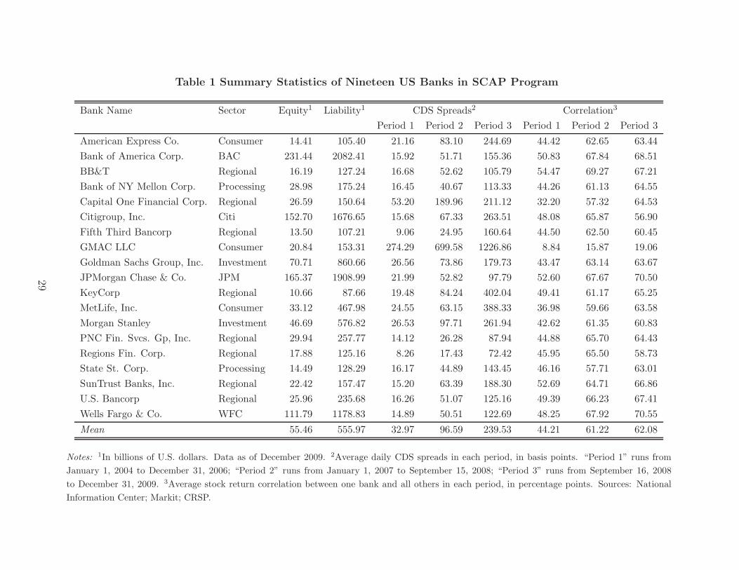
Table 1 Summary Statistics of Nineteen US Banks in SCAP Program

Bank Name Sector Equity1 Liability1 CDS Spreads2 Correlation3

Period 1 Period 2 Period 3 Period 1 Period 2 Period 3

American Express Co. Consumer 14.41 105.40 21.16 83.10 244.69 44.42 62.65 63.44

Bank of America Corp. BAC 231.44 2082.41 15.92 51.71 155.36 50.83 67.84 68.51

BB&T Regional 16.19 127.24 16.68 52.62 105.79 54.47 69.27 67.21

Bank of NY Mellon Corp. Processing 28.98 175.24 16.45 40.67 113.33 44.26 61.13 64.55

Capital One Financial Corp. Regional 26.59 150.64 53.20 189.96 211.12 32.20 57.32 64.53

Citigroup, Inc. Citi 152.70 1676.65 15.68 67.33 263.51 48.08 65.87 56.90

Fifth Third Bancorp Regional 13.50 107.21 9.06 24.95 160.64 44.50 62.50 60.45

GMAC LLC Consumer 20.84 153.31 274.29 699.58 1226.86 8.84 15.87 19.06

Goldman Sachs Group, Inc. Investment 70.71 860.66 26.56 73.86 179.73 43.47 63.14 63.67

JPMorgan Chase & Co. JPM 165.37 1908.99 21.99 52.82 97.79 52.60 67.67 70.50

KeyCorp Regional 10.66 87.66 19.48 84.24 402.04 49.41 61.17 65.25

MetLife, Inc. Consumer 33.12 467.98 24.55 63.15 388.33 36.98 59.66 63.58

Morgan Stanley Investment 46.69 576.82 26.53 97.71 261.94 42.62 61.35 60.83

PNC Fin. Svcs. Gp, Inc. Regional 29.94 257.77 14.12 26.28 87.94 44.88 65.70 64.43

Regions Fin. Corp. Regional 17.88 125.16 8.26 17.43 72.42 45.95 65.50 58.73

State St. Corp. Processing 14.49 128.29 16.17 44.89 143.45 46.16 57.71 63.01

SunTrust Banks, Inc. Regional 22.42 157.47 15.20 63.39 188.30 52.69 64.71 66.86

U.S. Bancorp Regional 25.96 235.68 16.26 51.07 125.16 49.39 66.23 67.41

Wells Fargo & Co. WFC 111.79 1178.83 14.89 50.51 122.69 48.25 67.92 70.55

Mean 55.46 555.97 32.97 96.59 239.53 44.21 61.22 62.08

Notes: 1In billions of U.S. dollars. Data as of December 2009. 2Average daily CDS spreads in each period, in basis points. “Period 1” runs from

January 1, 2004 to December 31, 2006; “Period 2” runs from January 1, 2007 to September 15, 2008; “Period 3” runs from September 16, 2008

to December 31, 2009. 3Average stock return correlation between one bank and all others in each period, in percentage points. Sources: National

Information Center; Markit; CRSP.

29

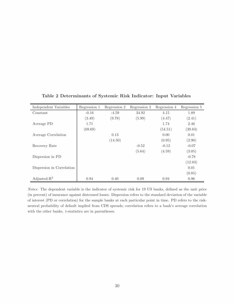
Table 2 Determinants of Systemic Risk Indicator: Input Variables

Independent Variables Regression 1 Regression 2 Regression 3 Regression 4 Regression 5

Constant -0.16 -4.59 34.92 4.15 1.89

(3.49) (9.78) (5.99) (4.47) (2.41)

Average PD 1.71 1.74 2.46

(69.69) (54.51) (39.83)

Average Correlation 0.13 0.00 0.01

(14.50) (0.95) (2.90)

Recovery Rate -0.52 -0.12 -0.07

(5.64) (4.59) (3.05)

Dispersion in PD -0.78

(12.83)

Dispersion in Correlation 0.01

(0.85)

Adjusted-R2 0.94 0.40 0.09 0.94 0.96

Notes: The dependent variable is the indicator of systemic risk for 19 US banks, defined as the unit price

(in percent) of insurance against distressed losses. Dispersion refers to the standard deviation of the variable

of interest (PD or correlation) for the sample banks at each particular point in time. PD refers to the risk-

neutral probability of default implied from CDS spreads; correlation refers to a bank’s average correlation

with the other banks. t-statistics are in parentheses.

30

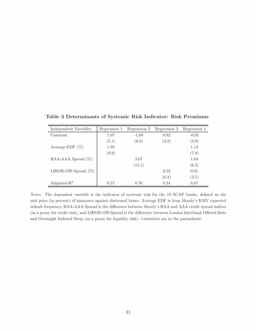
Table 3 Determinants of Systemic Risk Indicator: Risk Premiums

Independent Variables Regression 1 Regression 2 Regression 3 Regression 4

Constant 1.07 -1.68 0.92 -0.91

(5.1) (6.0) (3.2) (3.9)

Average EDF (%) 1.93 1.14

(9.8) (7.8)

BAA-AAA Spread (%) 3.07 1.64

(15.1) (6.2)

LIBOR-OIS Spread (%) 2.52 0.91

(6.2) (3.5)

Adjusted-R2 0.57 0.76 0.34 0.87

Notes: The dependent variable is the indicator of systemic risk for the 19 SCAP banks, defined as the

unit price (in percent) of insurance against distressed losses. Average EDF is from Moody’s KMV expected

default frequency, BAA-AAA Spread is the difference between Moody’s BAA and AAA credit spread indices

(as a proxy for credit risk), and LIBOR-OIS Spread is the difference between London Interbank Offered Rate

and Overnight Indexed Swap (as a proxy for liquidity risk). t-statistics are in the parenthesis.

31

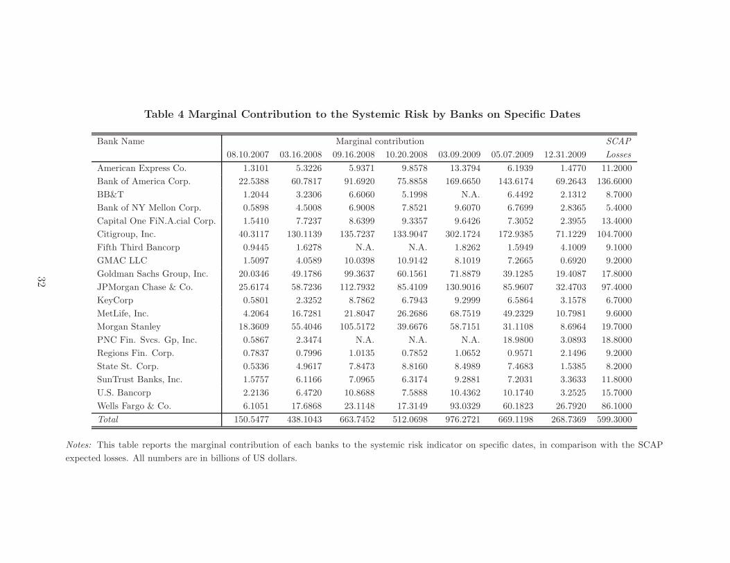
Table 4 Marginal Contribution to the Systemic Risk by Banks on Specific Dates

Bank Name Marginal contribution SCAP

08.10.2007 03.16.2008 09.16.2008 10.20.2008 03.09.2009 05.07.2009 12.31.2009 Losses

American Express Co. 1.3101 5.3226 5.9371 9.8578 13.3794 6.1939 1.4770 11.2000

Bank of America Corp. 22.5388 60.7817 91.6920 75.8858 169.6650 143.6174 69.2643 136.6000

BB&T 1.2044 3.2306 6.6060 5.1998 N.A. 6.4492 2.1312 8.7000

Bank of NY Mellon Corp. 0.5898 4.5008 6.9008 7.8521 9.6070 6.7699 2.8365 5.4000

Capital One FiN.A.cial Corp. 1.5410 7.7237 8.6399 9.3357 9.6426 7.3052 2.3955 13.4000

Citigroup, Inc. 40.3117 130.1139 135.7237 133.9047 302.1724 172.9385 71.1229 104.7000

Fifth Third Bancorp 0.9445 1.6278 N.A. N.A. 1.8262 1.5949 4.1009 9.1000

GMAC LLC 1.5097 4.0589 10.0398 10.9142 8.1019 7.2665 0.6920 9.2000

Goldman Sachs Group, Inc. 20.0346 49.1786 99.3637 60.1561 71.8879 39.1285 19.4087 17.8000

JPMorgan Chase & Co. 25.6174 58.7236 112.7932 85.4109 130.9016 85.9607 32.4703 97.4000

KeyCorp 0.5801 2.3252 8.7862 6.7943 9.2999 6.5864 3.1578 6.7000

MetLife, Inc. 4.2064 16.7281 21.8047 26.2686 68.7519 49.2329 10.7981 9.6000

Morgan Stanley 18.3609 55.4046 105.5172 39.6676 58.7151 31.1108 8.6964 19.7000

PNC Fin. Svcs. Gp, Inc. 0.5867 2.3474 N.A. N.A. N.A. 18.9800 3.0893 18.8000

Regions Fin. Corp. 0.7837 0.7996 1.0135 0.7852 1.0652 0.9571 2.1496 9.2000

State St. Corp. 0.5336 4.9617 7.8473 8.8160 8.4989 7.4683 1.5385 8.2000

SunTrust Banks, Inc. 1.5757 6.1166 7.0965 6.3174 9.2881 7.2031 3.3633 11.8000

U.S. Bancorp 2.2136 6.4720 10.8688 7.5888 10.4362 10.1740 3.2525 15.7000

Wells Fargo & Co. 6.1051 17.6868 23.1148 17.3149 93.0329 60.1823 26.7920 86.1000

Total 150.5477 438.1043 663.7452 512.0698 976.2721 669.1198 268.7369 599.3000

Notes: This table reports the marginal contribution of each banks to the systemic risk indicator on specific dates, in comparison with the SCAP

expected losses. All numbers are in billions of US dollars.

32

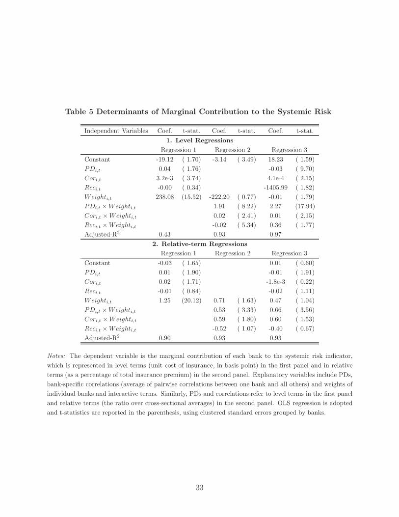
Table 5 Determinants of Marginal Contribution to the Systemic Risk

Independent Variables Coef. t-stat. Coef. t-stat. Coef. t-stat.

1. Level Regressions

Regression 1 Regression 2 Regression 3

Constant -19.12 ( 1.70) -3.14 ( 3.49) 18.23 ( 1.59)

PDi,t 0.04 ( 1.76) -0.03 ( 9.70)

Cori,t 3.2e-3 ( 3.74) 4.1e-4 ( 2.15)

Reci,t -0.00 ( 0.34) -1405.99 ( 1.82)

Weighti,t 238.08 (15.52) -222.20 ( 0.77) -0.01 ( 1.79)

PDi,t × Weighti,t 1.91 ( 8.22) 2.27 (17.94)

Cori,t × Weighti,t 0.02 ( 2.41) 0.01 ( 2.15)

Reci,t × Weighti,t -0.02 ( 5.34) 0.36 ( 1.77)

Adjusted-R2 0.43 0.93 0.97

2. Relative-term Regressions

Regression 1 Regression 2 Regression 3

Constant -0.03 ( 1.65) 0.01 ( 0.60)

PDi,t 0.01 ( 1.90) -0.01 ( 1.91)

Cori,t 0.02 ( 1.71) -1.8e-3 ( 0.22)

Reci,t -0.01 ( 0.84) -0.02 ( 1.11)

Weighti,t 1.25 (20.12) 0.71 ( 1.63) 0.47 ( 1.04)

PDi,t × Weighti,t 0.53 ( 3.33) 0.66 ( 3.56)

Cori,t × Weighti,t 0.59 ( 1.80) 0.60 ( 1.53)

Reci,t × Weighti,t -0.52 ( 1.07) -0.40 ( 0.67)

Adjusted-R2 0.90 0.93 0.93

Notes: The dependent variable is the marginal contribution of each bank to the systemic risk indicator,

which is represented in level terms (unit cost of insurance, in basis point) in the first panel and in relative

terms (as a percentage of total insurance premium) in the second panel. Explanatory variables include PDs,

bank-specific correlations (average of pairwise correlations between one bank and all others) and weights of

individual banks and interactive terms. Similarly, PDs and correlations refer to level terms in the first panel

and relative terms (the ratio over cross-sectional averages) in the second panel. OLS regression is adopted

and t-statistics are reported in the parenthesis, using clustered standard errors grouped by banks.

33

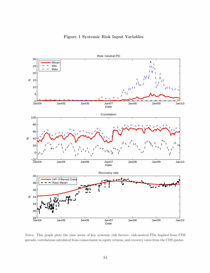
Figure 1 Systemic Risk Input Variables

Jan04 Jan05 Jan06 Jan07 Jan08 Jan09 Jan100

5

10

15

20

25

30

Date

%

Risk−neutral PD

MeanMinMax

Jan04 Jan05 Jan06 Jan07 Jan08 Jan09 Jan1028

30

32

34

36

38

40

Date

%

Recovery rate

HP−Filtered DataRaw Mean

Jan04 Jan05 Jan06 Jan07 Jan08 Jan09 Jan10−20

0

20

40

60

80

100

Date

%

Correlation

Notes: This graph plots the time series of key systemic risk factors: risk-neutral PDs implied from CDS

spreads, correlations calculated from comovement in equity returns, and recovery rates from the CDS quotes.

34

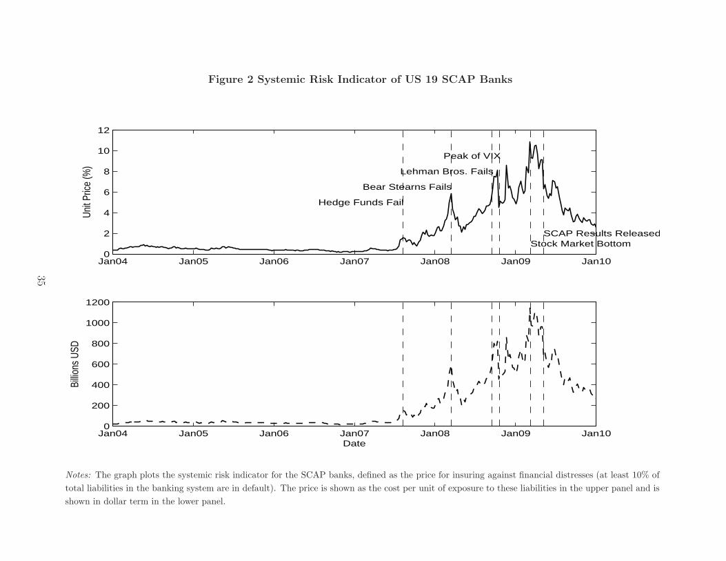
Figure 2 Systemic Risk Indicator of US 19 SCAP Banks

Jan04 Jan05 Jan06 Jan07 Jan08 Jan09 Jan100

2

4

6

8

10

12

Unit

Price

(%)

Hedge Funds Fail

Bear Stearns Fails

Lehman Bros. Fails

Peak of VIX

Stock Market BottomSCAP Results Released

Jan04 Jan05 Jan06 Jan07 Jan08 Jan09 Jan100

200

400

600

800

1000

1200

Billio

ns U

SD

Date

Notes: The graph plots the systemic risk indicator for the SCAP banks, defined as the price for insuring against financial distresses (at least 10% of

total liabilities in the banking system are in default). The price is shown as the cost per unit of exposure to these liabilities in the upper panel and is

shown in dollar term in the lower panel.

35

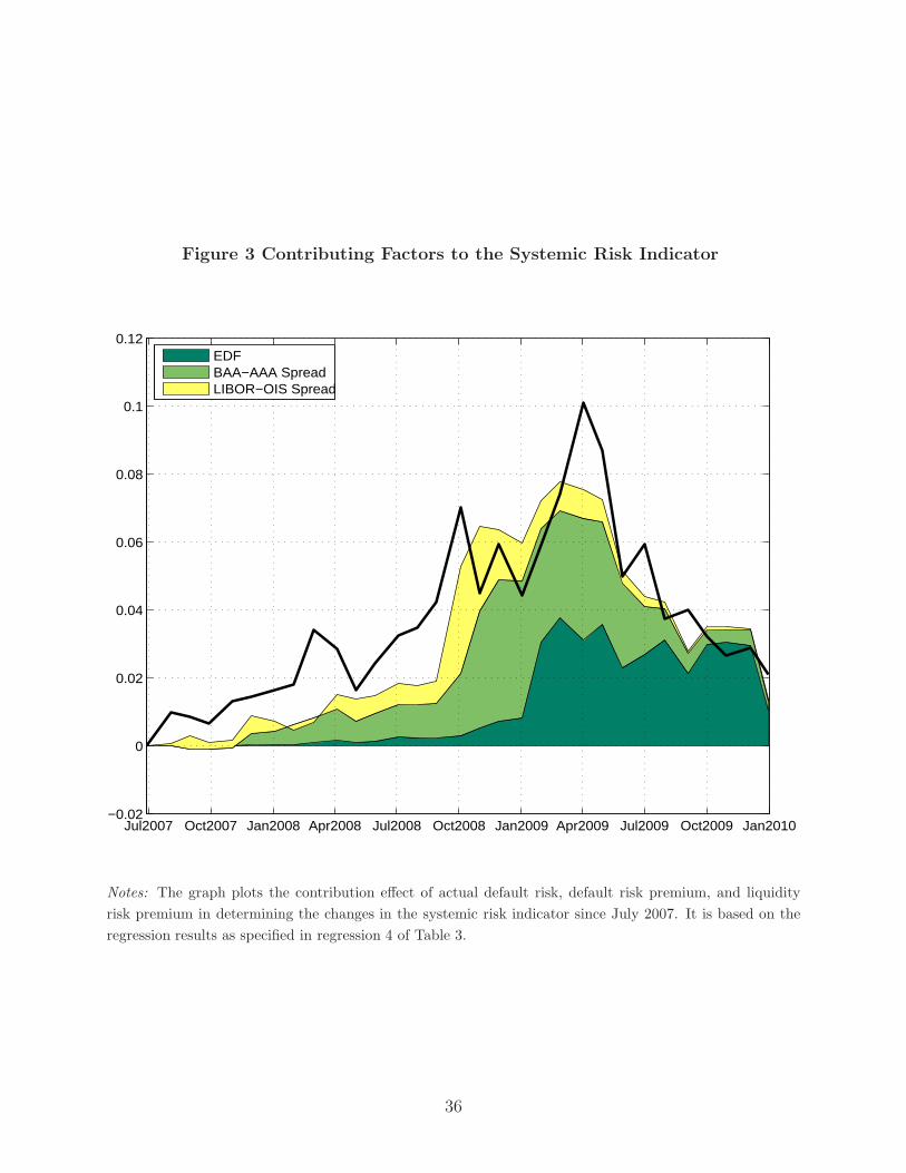
Figure 3 Contributing Factors to the Systemic Risk Indicator

Jul2007 Oct2007 Jan2008 Apr2008 Jul2008 Oct2008 Jan2009 Apr2009 Jul2009 Oct2009 Jan2010−0.02

0

0.02

0.04

0.06

0.08

0.1

0.12EDFBAA−AAA SpreadLIBOR−OIS Spread

Notes: The graph plots the contribution effect of actual default risk, default risk premium, and liquidity

risk premium in determining the changes in the systemic risk indicator since July 2007. It is based on the

regression results as specified in regression 4 of Table 3.

36

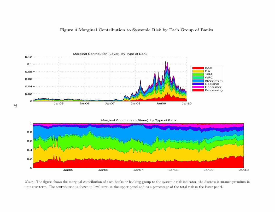
Figure 4 Marginal Contribution to Systemic Risk by Each Group of Banks

Jan05 Jan06 Jan07 Jan08 Jan09 Jan100

0.02

0.04

0.06

0.08

0.1

0.12Marginal Contribution (Level), by Type of Bank

BACCitiJPMWFCInvestmentRegionalConsumerProcessing

Jan05 Jan06 Jan07 Jan08 Jan09 Jan100

0.2

0.4

0.6

0.8

1Marginal Contribution (Share), by Type of Bank

Notes: The figure shows the marginal contribution of each banks or banking group to the systemic risk indicator, the distress insurance premium in

unit cost term. The contribution is shown in level term in the upper panel and as a percentage of the total risk in the lower panel.

37

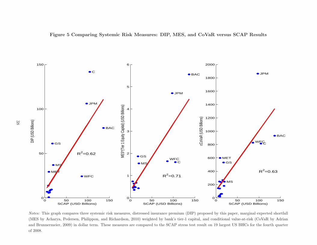
Figure 5 Comparing Systemic Risk Measures: DIP, MES, and CoVaR versus SCAP Results

0 50 100 1500

50

100

150

SCAP (USD Billions)

DIP

(USD

Billi

ons)

BAC

C

GS

JPM

MET

MS

WFC

R2=0.62

0 50 100 1500

1

2

3

4

5

6

SCAP (USD Billions)

MES*

(Tier

1 Eq

uity C

apita

l) (US

D Bi

llions

)

BAC

C

GS

JPM

MS

WFC

R2=0.71

0 50 100 1500

200

400

600

800

1000

1200

1400

1600

1800

2000

SCAP (USD Billions)cC

oVaR

(USD

Billi

ons)

BAC

C

GS

JPM

MET

MS

WFC

R2=0.63

Notes: This graph compares three systemic risk measures, distressed insurance premium (DIP) proposed by this paper, marginal expected shortfall

(MES by Acharya, Pedersen, Philippon, and Richardson, 2010) weighted by bank’s tier-1 capital, and conditional value-at-risk (CoVaR by Adrian

and Brunnermeier, 2009) in dollar term. These measures are compared to the SCAP stress test result on 19 largest US BHCs for the fourth quarter

of 2008.

38

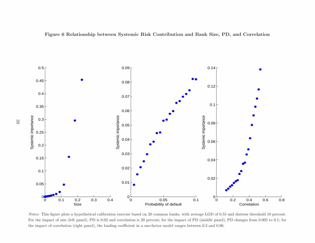
Figure 6 Relationship between Systemic Risk Contribution and Bank Size, PD, and Correlation

0 0.1 0.2 0.3 0.40

0.05

0.1

0.15

0.2

0.25

0.3

0.35

0.4

0.45

0.5

Size

Sys

tem

ic im

porta

nce

0 0.05 0.10

0.01

0.02

0.03

0.04

0.05

0.06

0.07

0.08

0.09

Probability of default

Sys

tem

ic im

porta

nce

0 0.2 0.4 0.6 0.80

0.02

0.04

0.06

0.08

0.1

0.12

0.14

CorrelationS

yste

mic

impo

rtanc

e

Notes: This figure plots a hypothetical calibration exercise based on 20 common banks, with average LGD of 0.55 and distress threshold 10 percent.

For the impact of size (left panel), PD is 0.02 and correlation is 20 percent; for the impact of PD (middle panel), PD changes from 0.005 to 0.1; for

the impact of correlation (right panel), the loading coefficient in a one-factor model ranges between 0.2 and 0.96.

39