Finance and Economics Discussion SeriesDivisions of Research & Statistics and Monetary Affairs

Federal Reserve Board, Washington, D.C.

Two Practical Algorithms for Solving Rational ExpectationsModels

Flint Brayton

2011-44

NOTE: Staff working papers in the Finance and Economics Discussion Series (FEDS) are preliminarymaterials circulated to stimulate discussion and critical comment. The analysis and conclusions set forthare those of the authors and do not indicate concurrence by other members of the research staff or theBoard of Governors. References in publications to the Finance and Economics Discussion Series (other thanacknowledgement) should be cleared with the author(s) to protect the tentative character of these papers.

Two Practical Algorithms for SolvingRational Expectations Models ∗

Flint Brayton

Federal Reserve Board

October 11, 2011

Abstract

This paper describes the E-Newton and E-QNewton algorithms for solvingrational expectations (RE) models. Both algorithms treat a model’s REterms as exogenous variables whose values are iteratively updated until they(hopefully) satisfy the RE requirement. In E-Newton, the updates are basedon Newton’s method; E-QNewton uses an efficient form of Broyden’s quasi-Newton method. The paper shows that the algorithms are reliable, fastenough for practical use on a mid-range PC, and simple enough that theirimplementation does not require highly specialized software. The evalua-tion of the algorithms is based on experiments with three well-known macromodels—the Smets-Wouters (SW) model, EDO, and FRB/US—using codewritten in EViews, a general-purpose, easy-to-use software package. Themodels are either linear (SW and EDO) or mildly nonlinear (FRB/US). Atest of the robustness of the algorithms in the presence of substantial nonlin-earity is based on modified versions of each model that include a smoothedform of the constraint that the short-term interest rate cannot fall below zero.In two single-simulation experiments with the standard and modified versionsof the models, E-QNewton is found to be faster than E-Newton, except forsolutions of small-to-medium sized linear models. In a multi-simulation ex-periment using the standard versions of the models, E-Newton dominatesE-QNewton.

∗email: Flint.Brayton@frb.gov. I thank John Roberts for helpful comments andMichael Kiley and Peter Chen for assistance with creating the EViews version of EDO.The views expressed in this paper are those of the author and do not necessarily representthe opinions of the Federal Reserve Board or its staff.

2

1. Introduction

This paper describes the E-Newton and E-QNewton algorithms for solv-

ing rational expectations (RE) models. Like the Fair-Taylor (FT) procedure

(Fair and Taylor, 1983), both algorithms treat a model’s RE terms as ex-

ogenous variables whose values are iteratively updated until they (hopefully)

satisfy the RE requirement.1 To improve solution speed and reliability, the

E-Newton algorithm replaces FT’s rudimentary updating mechanism with

one based on Newton’s method. In this respect, E-Newton is related to

the Newton-based stacked-time procedures that are now more widely used

than FT for solving nonlinear RE models.2 The expectations updates in the

E-QNewton algorithm use a quasi-Newton method. This paper shows that

the E-Newton and E-QNewton algorithms are not only practical and reliable,

but also that they are relatively simple to program and thus do not require

highly specialized software. For several years, solutions of the RE versions of

the Federal Reserve Board’s nonlinear FRB/US macroeconomic model have

been computed using code for the E-Newton algorithm written in EViews, a

general-purpose, easy-to-use software package. The E-QNewton algorithm,

which has been developed more recently, is also written in EViews.

The term rational expectations is used here to describe the condition in

which expectations of future values are identical to a model’s future solutions

in the absence of unexpected shocks. That is, there are no expectations

errors. For the algorithms described in this paper, the RE solution of a

model with m expectations variables for T periods involves finding the mT

expectations values that set a like number of expectations errors are zero. The

FT algorithm tackles this task with a simple mechanism that is equivalent

1The “E-” prefix attached to the names of the algorithms signifies the central role ofthe expectations estimates in the iteration process.

2Stacked-time algorithms, which impose the RE requirement by solving all time periodsin a simulation simultaneously, iterate on the values of all endogenous variables. Newtonversions of stacked time are described in Hollinger (1996) and Juillard (1996).

3

to updating at each iteration the estimate of each expected future value

in isolation, using only its own expectations error. In contrast, E-Newton

and E-QNewton update all mT expectations simultaneously, based on all

mT expectations errors and information on the relationship between the

expectations estimates and errors. In E-Newton this information takes the

form of the Jacobian matrix of first derivatives of the expectations errors

with respect to the expectations estimates. E-QNewton uses an approximate

Jacobian that is more easily calculated but less accurate than the Newton

Jacobian. The relative speed of the two algorithms in solving a particular RE

model depends on the model-specific cost trade-off between the accuracy of

the Jacobian and the number of iterations needed to achieve an RE solution.

E-Newton runs a set of impulse-response simulations (dynamic multipli-

ers) to compute the values of the derivatives that enter the Jacobian and

then inverts this matrix. These operations can be quite costly if the size of

the Jacobian, mT , is large, especially because the time required to invert a

matrix depends on the cube of its size. In fact, when an algorithm similar to

E-Newton was developed by Holly and Zarrop (1983) many years ago, these

costs were judged to be prohibitive for most RE models.3 Although the vast

advances in computation power over the past three decades have greatly di-

minished the importance of this judgment, the Jacobian costs in E-Newton

can nonetheless be substantial for larger RE models. In such cases, faster

solutions may be obtained with a quasi-Newton method, because it does

not require the explicit calculation of derivatives and can be set up to run

without inverting matrices. The E-QNewton algorithm uses a version of the

quasi-Newton method of Broyden (1965) that is described by Kelley (1995).

In E-QNewton, execution time is more sensitive to the number of solution

iterations than to the size of the Jacobian.

3Hall (1985) and Fisher (1992) discuss the efficiency and practicality of the Holly-Zarrop“penalty function” algorithm.

4

Newton and quasi-Newton methods are used to solve systems of equa-

tions that arise in many scientific disciplines. As this paper will show, the

efficiency of these methods when applied to solving RE models can be im-

proved by taking advantage of some characteristics that are common to many

models of this type. The cost of computing the E-Newton Jacobian can be

greatly reduced for many linear and mildly nonlinear RE models through the

use of shortcuts that take account of repetitive patterns in their derivatives.

In the E-QNewton algorithm, the accuracy of the approximate Jacobian can

be improved for most RE models by choosing a very specific initial approxi-

mation that is easily calculated.

Section 2 describes the E-Newton and E-QNewton algorithms. Section 3

briefly discusses the three well-known macro models that are used to evaluate

the performance of the algorithms: the Smets-Wouters (SW) model, EDO,

and FRB/US. SW and EDO are linear DSGE models; FRB/US is mildly

nonlinear. Each model is of medium size or larger. To test the algorithms

with models that are substantially nonlinear, an alternative version of each

model is created that includes a nonlinear but smooth approximation to the

constraint that the short-term interest rate cannot fall below zero.

The evaluation of the algorithms in section 4 is based on three simulation

experiments. The first is a one-time shock to each model’s interest rate

policy rule. The second is a shock that reduces output sufficiently to cause

the response of the short-term interest rate to be constrained by the zero

bound. The third experiment, which requires the execution of a set of RE

simulations, assumes that monetary policy responds to a shock by minimizing

a loss function.

The first two experiments suggest several conclusions. First, for single

simulations of linear RE models, E-Newton is likely to be faster for mod-

els of small-to-medium size (mT < 2000) and E-QNewton is likely to be

faster for larger models. Second, for nonlinear models, E-Newton tends to

5

be penalized relative to E-QNewton to the extent that the nonlinearity elim-

inates exploitable patterns among the derivatives in the Newton Jacobian.

In the specific case of the single-simulation experiment with the zero bound,

E-QNewton solves all of the models more rapidly than E-Newton. Third,

actual solution times support the claim that the algorithms are sufficiently

fast for practical use in many applications. With a mid-range PC, the fastest

execution time for each model in each experiment ranges from 0.3 seconds for

a stripped-down version of SW in the interest-rate experiment to 13.4 sec-

onds for the version of FRB/US in which all 27 of its expectations variables

have RE solutions in the zero-bound experiment.

The E-Newton algorithm has a substantial advantage over E-QNewton

on experiments that involve a large number of RE solutions, as long as the

same Jacobian can be used for each E-Newton solution. This Jacobian con-

dition is satisfied by each of the models in the third experiment, which is

designed so that the zero bound is not an issue. This optimal-policy simu-

lation, which entails 42 RE solutions for the linear models (SW and EDO)

and 131 RE solutions for FRB/US, executes between 2.2 and 18 times faster

with E-Newton than with E-QNewton, depending on the model.

For purposes of comparison, solutions of SW and EDO for the first two

experiments were also executed with the stacked-time algorithm in Dynare, a

specialized software language for RE models. The Octave-based Dynare solu-

tion times are similar to the best of each model’s E-Newton and E-QNewton

runs. Had they been run in Matlab, the Dynare solutions would likely have

been somewhat faster than the E-Newton and E-QNewton runs but not dra-

matically so. This suggests that many users may find the added solution time

of using the algorithms described here in a software language like EViews to

be more than offset by the many features available in such a general-purpose

environment that facilitate its use.

6

2. The Algorithms

This section of the paper, which may be skipped by the reader who is

less interested in technical details, has four parts. The first part summarizes

the algorithms. The second part examines in more detail the E-Newton

Jacobian and the shortcuts that can be used to speed up its construction.

The third part describes the E-QNewton approximate Jacobian and a pair of

transformations that enable it to be efficiently used. The last part discusses

convergence properties. Additional information on the algorithms is provided

in the Appendix.

2a. Overview

Consider a model of n equations in which f = [f1, . . . fn]′ is a vector-

valued function of n endogenous variables, yt = [y1,t, . . . yn,t]′.

f(yt−1, yt, yt+1) =

f1(yt−1, yt, yt+1)...

fn(yt−1, yt, yt+1)

= 0 (1)

For expositional simplicity, the model contains only a single lag and single

lead of y and exogenous variables are not shown. The lead term captures

the model’s RE expectations variables. The E-Newton and E-QNewton al-

gorithms (and FT, as well) replace yt+1 with an exogenous estimate of ex-

pectations, denoted by xt,

f(yt−1, yt, xt) = 0. (2)

The algorithms execute one or more iterations, each of which starts with a

solution of (2) for a given set of expectations estimates. The resulting values

of the RE expectations errors, et,

7

et = xt − yt+1. (3)

are then computed, taking as given the value of yt+1 obtained in solving (2).

Depending on the size of the errors, the solution of equations 2-3 may be

repeated with a different step length, in which the expectations estimates

are moved either back toward or farther from their values in the previous

iteration. Lastly, a set of revised expectations estimates is constructed for

use in the next iteration.

Some additional notation is needed to describe how the expectations es-

timates are revised in the last step of each iteration. Assume a solution for

t = 1, . . . , T , and stack the vectors of the expectations estimates and expec-

tations errors for all T time periods in x and e, respectively. If there are m

distinct expectations variables, e and x are vectors of length mT . The rela-

tionship between these two stacked vectors can be written in general terms

as

e = F (x), (4)

where the function F is a compact representation of the model’s structure,

also in stacked form.4 Using this representation, the condition that expecta-

tions are rational,

F (x) = 0, (5)

is the solution of a system of (possibly) nonlinear equations. Each evaluation

of F requires a simulation of the model given by equations 2-3.

4F also depends on the initial and terminal values of y.

8

The field of numerical analysis contains many algorithms for solving sys-

tems of nonlinear equations. Some of these algorithms characterize the ad-

justment of x at iteration i as the product of a step length, λi, and a direction,

di,

∆xi = λidi, (6)

where the direction in turn depends on the product of an updating matrix

U and the value of F in the previous iteration,

di = −Ui−1F (xi−1). (7)

The iterations of E-Newton and E-QNewton can be expressed in the form of

equations 6-7, differing only in how U is defined. The FT algorithm is the

special case in which U is the identity matrix.

When Newton’s method is used to solve a system of equations, the up-

dating matrix is the inverse of the Jacobian matrix of first derivatives (J =

(∂F/∂x)). In E-Newton specifically, J is the matrix of derivatives of the

expectations errors with respect to the expectations estimates.5

When quasi-Newton methods are used to solve systems of equations, the

updating matrix is the inverse of an approximate Jacobian (B) whose ele-

ments are based only on the implicit derivative information observed each

iteration in the movements of F and x. Quasi-Newton methods do not calcu-

late derivatives explicitly. Rather, starting from some initial estimate (B0),

they revise the approximate Jacobian each iteration so that it matches the

slope of F revealed in the previous iteration in the particular direction that

5Note the distinction between the RE Jacobian, J , which is associated with equation 5,and the structural Jacobian of the original RE model in equation 1. The iterations ofthe Newton-based stacked-time algorithm make use of a stacked form of the structuralJacobian.

9

x was adjusted. Many matrix updating formulas satisfy this condition. The

E-QNewton algorithm is based on the widely used method of Broyden (1965),

whose updating formula is the one that makes the smallest possible change

to the approximate Jacobian each iteration.6

2b. The E-Newton Jacobian

The most important and costly part of the E-Newton algorithm is the

computation and inversion of the Jacobian (J). The algorithm executes

impulse-response simulations (dynamic multipliers) of the model formed by

equations 2-3 to compute J . Although mT impulse-response simulations

may be needed for this purpose at each iteration (one for each expectations

variable in each simulation period), models that are linear or mildly nonlinear

require many fewer simulations.

The Jacobian of a linear RE model has a repetitive structure. This is

illustrated with a single-equation RE model in which the variable y depends

only on its first lead and first lag,

yt = αyt−1 + βyt+1 + ǫt. (8)

Define the operational model using xt to represent the expectations estimate

and et the expectations error.

yt = αyt−1 + βxt + ǫt (9)

et = xt − yt+1 (10)

Repeated substitution of (9) into (10) yields the following equation,

6The change in the approximate Jacobian is defined in terms of its norm: ||Bi−Bi−1||.

10

et =

xt −∑t−1

i=−1 αi+1(βxt−i + ǫt−i)− αt+1y0 t < T

xT − yT+1 t = T(11)

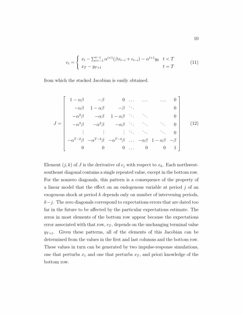
from which the stacked Jacobian is easily obtained.

J =

1− αβ −β 0 . . . . . . . . . 0

−αβ 1− αβ −β. . . 0

−α2β −αβ 1− αβ. . . . . . 0

−α3β −α2β −αβ. . . . . . . . . 0

......

.... . . . . . . . . 0

−αT−2β −αT−3β −αT−4β . . . −αβ 1− αβ −β

0 0 0 . . . 0 0 1

(12)

Element (j, k) of J is the derivative of ej with respect to xk. Each northwest-

southeast diagonal contains a single repeated value, except in the bottom row.

For the nonzero diagonals, this pattern is a consequence of the property of

a linear model that the effect on an endogenous variable at period j of an

exogenous shock at period k depends only on number of intervening periods,

k−j. The zero diagonals correspond to expectations errors that are dated too

far in the future to be affected by the particular expectations estimate. The

zeros in most elements of the bottom row appear because the expectations

error associated with that row, eT , depends on the unchanging terminal value

yT+1. Given these patterns, all of the elements of this Jacobian can be

determined from the values in the first and last columns and the bottom row.

These values in turn can be generated by two impulse-response simulations,

one that perturbs x1 and one that perturbs xT , and priori knowledge of the

bottom row.

11

A simple generalization of this single-equation Jacobian holds for all lin-

ear RE models in which expectations are formed at time t for outcomes at

t + 1. The Jacobians of such models, which consist of m2 blocks, each of

which is similar to (12), can be calculated with only 2m impulse response

simulations and priori knowledge of the bottom row of each Jacobian block.

For qualifying models, this shortcut greatly speeds up the computation of

the Jacobian.7

The cost of computing the Jacobian can also be reduced for models

that are mildly nonlinear. Although the Jacobian blocks of such models

do not have constant diagonals, the values along each diagonal may shift

relatively smoothly. Useful approximations to these Jacobian can usually be

constructed by calculating a subset of the columns with impulse-response

simulations and estimating the values in the other columns by linear inter-

polation along the diagonals.

2c. The E-QNewton approximate Jacobian

Define the step si as the change from the previous iteration of x and

zi as the resulting change of F . In the RE context, si is the change in

the expectations estimates and F is the change in the expectations errors.

With these definitions, the revision to the approximate Jacobian in Broyden’s

method can be expressed as,

Bi = Bi−1 +zi −Bi−1si

s′isis′i. (13)

Some intuition about this formula is obtained by noting that the revision to

7Some linear RE models contain expectations of outcomes dated more than one pe-riod in the future or form expectations only on the basis of lagged information. Thesemodifications alter the repetitive structure of the Jacobian blocks in specific ways. Withthe first modification, more than one diagonal above the main diagonal contains non-zeroentries, and more than one row at the bottom has entries that differ from the pattern inthe rows above. The assumption of lagged expectations modifies the right-hand columnsof the Jacobian blocks.

12

B depends on the vector (zi−Bi−1si), which measures how much the change

in F differs from what would have occurred if Bi−1 had in fact been the true

Jacobian.

Although it avoids the cost of computing explicit derivatives, the Broy-

den formula given by (13) has practical drawbacks in applications whose

approximate Jacobians are large and that require many iterations to solve:

To compute the adjustment direction each iteration, B needs to be inverted

and then multiplied by F (x). However, two transformations lead to a formula

that executes much more quickly in these cases. The first transformation uses

the Sherman-Morrison formula to convert (13) into an expression for directly

updating the inverse of the approximate Jacobian.

B−1i = B−1

i−1 +si −B−1

i−1zis′iB

−1i−1zi

(s′iB−1i−1). (14)

The second transformation recognizes that the expression B−1i F (xi) can be

expressed as a function of the product of the inverse of the initial approx-

imate Jacobian and F (xi), and the iteration histories of revisions to the

expectations estimates and step lengths.

B−1i F (xi) = G(s1, s2, . . . , si, λ1, λ2, . . . , λi)B

−10 F (xi) (15)

As long as i is not too large relative to mT and B−10 has a simple form, it

can be considerably faster to compute the adjustment direction using (15)

than by the two-step process of forming B−1i from (14) and multiplying the

result by F (xi).8

8The transformation embodied in (15) is taken from Kelley (1995, chapters 7-8). Thespecific form of the function G is presented in the Appendix. As shown in Appendixtable A1, the second transformation reduces solution time between 32 and 97 percent,depending on the model and the simulation experiment.

13

Before it starts, the E-QNewton algorithm requires an initial approxi-

mate Jacobian, B0. The conventional recommendation is to use the identity

matrix, a choice that, because it has the effect of eliminating all matrices

from (15), causes each iteration to execute very quickly. As a general mat-

ter, the choice of B0 has to balance two considerations: A simpler estimate

speeds up each iteration, while a more accurate estimate reduces the num-

ber of iterations required for convergence. For most of the models examined

here, a simplified, block-diagonal estimate of the Jacobian, calculated from

m impulse response simulations (one per RE variable), is usually a better

choice than the identity matrix. Because this matrix, Bbd0 , has an inverse

that can be easily computed and stored compactly in m TxT matrices, its

use increases computation time per iteration only modestly relative to that

for B0 = I. At the same time, the improvement in the accuracy of the ini-

tial approximate Jacobian is such that the benefit of fewer iterations greatly

outweighs the higher cost per iteration in most cases.

2d. Convergence and the step length

The adjustment of the expectations estimates each iteration is the prod-

uct of the step direction (d) and the step length (λ). Thus far, the detailed

discussion of the two algorithms has concentrated on the E-Newton Jacobian

and the E-QNewton approximate Jacobian, matrices that enter the compu-

tation of the direction. With regard to the step length, algorithms that use

the Newton or quasi-Newton directions always converge to the solutions of

linear models when λ=1.0.9 With this step length, E-Newton solutions re-

quire a single iteration, as long as the Jacobian is exactly computed, and

E-QNewton solutions require at most 2mT iterations.10

9This statement requires several qualifications. The Newton Jacobian or the quasi-Newton approximate Jacobian must be non-singular. The statement does not apply tothe E-Newton algorithm when it uses an inexact Jacobian. For an RE model that doesnot satisfy the Blanchard-Kahn conditions, the solution obtained may not be economicallymeaningful.

10The E-QNewton convergence results are based on Gay (1979), who proves that Broy-

14

A step length of 1.0 does not guarantee the convergence of E-Newton

or E-QNewton to the solution of a nonlinear RE model, unless the starting

point is close to the solution. For nonlinear models, the convergence proper-

ties of the pair of algorithms is improved if line-search procedures are used

to examine alternative step lengths, whenever the default length (λ = 1,

typically) yields an insufficient movement toward the RE solution. The ratio

of the sum of squared expectations errors in successive iterations,

g(xi) =e′iei

e′i−1ei−1

, (16)

provides a scalar measure of the iteration-by-iteration progress.

E-Newton uses the relatively simple Armijo line-search procedure in which

the step length starts at 1.0 and then is repeatedly shortened, if necessary, un-

til either g(xi) < (1−λiγ) or the maximum number of step-length iterations

is reached.11 In E-Newton, γ = .01, the step length shortening parameter is

0.5, and the maximum number of line-search iterations is ten.

For quasi-Newton methods, the decision of how intensively to search for

the best step length each iteration is more complex than in the Newton case,

because even an iteration that fails to make much or any progress toward

the RE solution is still likely to improve the accuracy of the approximate

Jacobian to be used in the next iteration. In particular, it may be more

efficient to move on to the next iteration than to try to refine the step length

in the current iteration, when the direction in which x is being adjusted is

likely to make little progress. For this reason, E-QNewton uses the non-

monotone step-length procedure of La Cruz, Martinez, and Raydan (LMR,

den’s method always converges to the solution of a linear system of equations when thestep length is 1.0, and that the required number of iterations never exceeds twice thenumber of equations.

11Kelley (1995, pp. 138-141) describes the conditions under which the Armijo procedureis globally convergent.

15

2005). This procedure tolerates temporary, limited increases in the sum of

squared expectations errors, g(xi) > 1, without searching for a better step

length, especially in the initial solution iterations, when the accuracy of the

approximate Jacobian and the adjustment direction is likely to be worst. In

addition, the LMR procedure tests both positive and negative step lengths,

a feature that is useful when the direction is so poor that no positive step

length reduces the sum of squared expectations errors.

Both E-Newton and E-QNewton have much better convergence properties

than FT. All of models considered here converge to their RE solutions in all of

the experiments for at least one of the E-Newton Jacobian options and for at

least one of the E-QNewton options for initializing the approximate Jacobian,

using the line-search algorithms just discussed when appropriate. In contrast,

the FT algorithm does not have a high rate of successful convergence for

these specific models, a result which can be shown using a simple condition

provided by this paper’s RE solution framework.12

For a linear model, the evolution of the expectations errors depends on

the Jacobian and the expectations estimates.

ei = ei−1 + J [xi − xi−1] (17)

= (I − λJ)ei−1 (18)

The derivation of (18) uses the version of (7) that holds under FT to sub-

stitute for the change in the expectations estimates. FT convergence of e to

zero thus requires that the eigenvalues of (I − λJ) lie inside the unit circle.

12For a summary of convergence problems that have been encountered when using FTto solve other RE macro models, see Juillard et. al. (1999), who report that nine of 13macro modelers surveyed had difficulties with FT and similar algorithms in cases where thestacked-time algorithm worked. Because they are both Newton methods, the convergenceproperties of E-Newton and stacked-time should be similar.

16

Related to this is a second condition that requires all of the eigenvalues of

(I−J) to be less than 1.0 for there to exist some λ > 0 that satisfies the first

condition.13 Of the linear models used in this paper, EDO satisfies the sec-

ond FT convergence condition but SW does not. For nonlinear models, FT

convergence requires that the second condition hold in some neighborhood

of the solution. This is satisfied by the simpler version of FRB/US but not

by the one in which all 27 of its expectations variables have RE solutions.

3. The Models

Three models are used to evaluate the E-Newton and E-QNewton algo-

rithms. One model is the well-known New-Keynesian DSGE of Smets and

Wouters (2007). The other two models are ones developed and used at the

Federal Reserve Board: EDO and FRB/US. EDO is a New-Keynesian DSGE

that is considerably larger than Smets-Wouters (SW).14 FRB/US, which is an

even larger model, also has New-Keynesian characteristics, but its structure

is estimated with fewer constraints than a DSGE framework would impose.15

Several versions of each model are employed. A small version of SW (SW-

small) eliminates the flexible-price concept of potential output, a change that

permits several equations to be dropped but requires that the interest-rate

equation be modified to depend on the log level of output rather than on

the output gap. One version of FRB/US assumes that all of its expecta-

tions variables have RE solutions (FRB/US-all); in a second version, only

those expectations that appear in asset-pricing equations have RE solutions

(FRB/US-mcap).16

13For other representations of the first FT convergence condition, see Fisher and HughesHallett (1988) and Armstrong, et. al. (1998). The relationship between convergenceconditions of the first and second type is described in Fisher and Hughes Hallett (1988).

14EDO is described in Chung, et.al. (2010) and Edge, et.al. (2008).15FRB/US is described in Brayton and Tinsley (1996) and Brayton, et.al. (1997a).16MCAP: Model-Consistent Asset Pricing.

17

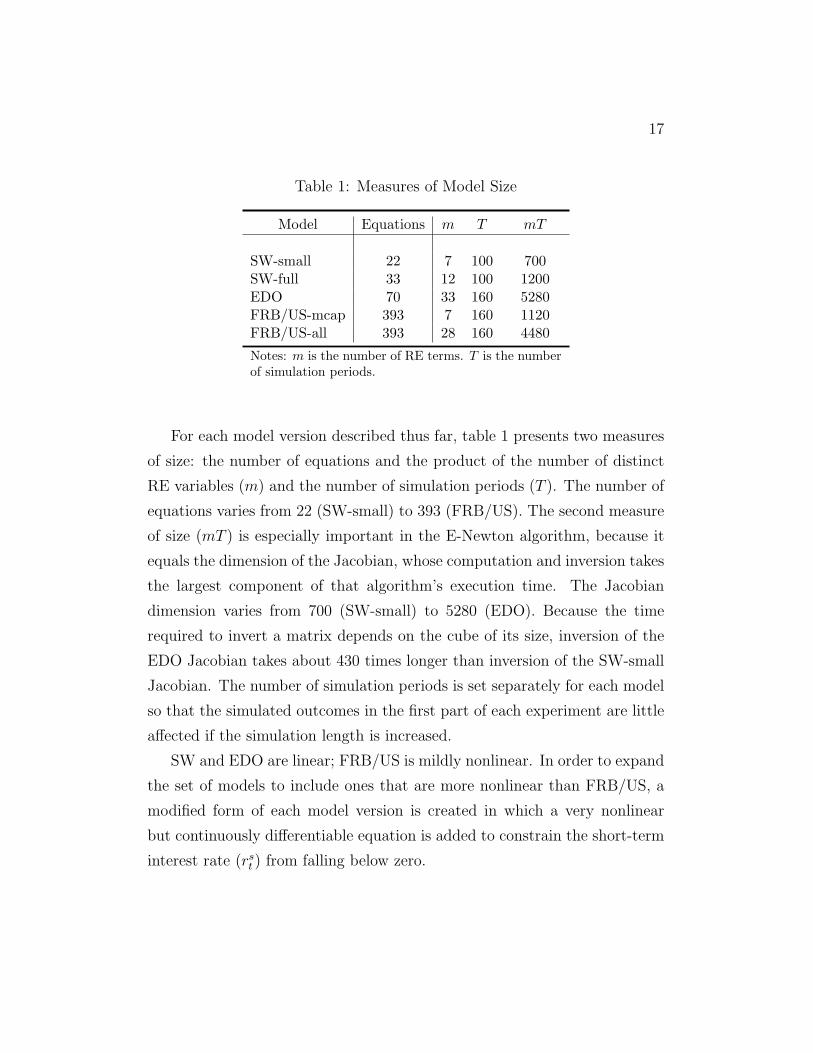
Table 1: Measures of Model Size

Model Equations m T mT

SW-small 22 7 100 700SW-full 33 12 100 1200EDO 70 33 160 5280FRB/US-mcap 393 7 160 1120FRB/US-all 393 28 160 4480

Notes: m is the number of RE terms. T is the numberof simulation periods.

For each model version described thus far, table 1 presents two measures

of size: the number of equations and the product of the number of distinct

RE variables (m) and the number of simulation periods (T ). The number of

equations varies from 22 (SW-small) to 393 (FRB/US). The second measure

of size (mT ) is especially important in the E-Newton algorithm, because it

equals the dimension of the Jacobian, whose computation and inversion takes

the largest component of that algorithm’s execution time. The Jacobian

dimension varies from 700 (SW-small) to 5280 (EDO). Because the time

required to invert a matrix depends on the cube of its size, inversion of the

EDO Jacobian takes about 430 times longer than inversion of the SW-small

Jacobian. The number of simulation periods is set separately for each model

so that the simulated outcomes in the first part of each experiment are little

affected if the simulation length is increased.

SW and EDO are linear; FRB/US is mildly nonlinear. In order to expand

the set of models to include ones that are more nonlinear than FRB/US, a

modified form of each model version is created in which a very nonlinear

but continuously differentiable equation is added to constrain the short-term

interest rate (rst ) from falling below zero.

18

.0

.1

.2

.3

.4

.5

.6

-.5 -.4 -.3 -.2 -.1 .0 .1 .2 .3 .4 .5

Unconstrained rate of interest

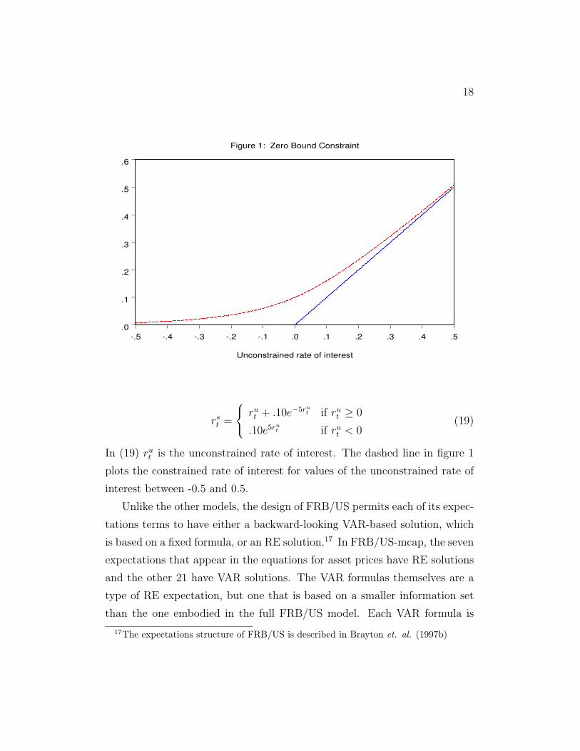
Figure 1: Zero Bound Constraint

rst =

rut + .10e−5rut if rut ≥ 0

.10e5rut if rut < 0

(19)

In (19) rut is the unconstrained rate of interest. The dashed line in figure 1

plots the constrained rate of interest for values of the unconstrained rate of

interest between -0.5 and 0.5.

Unlike the other models, the design of FRB/US permits each of its expec-

tations terms to have either a backward-looking VAR-based solution, which

is based on a fixed formula, or an RE solution.17 In FRB/US-mcap, the seven

expectations that appear in the equations for asset prices have RE solutions

and the other 21 have VAR solutions. The VAR formulas themselves are a

type of RE expectation, but one that is based on a smaller information set

than the one embodied in the full FRB/US model. Each VAR formula is

17The expectations structure of FRB/US is described in Brayton et. al. (1997b)

19

derived as part of the sector-by-sector estimation of FRB/US, which relies

on small models that combine one or a few structural equations with several

VAR relationships.18

4. Simulation Experiments

One of the purposes of this paper is to show that the E-Newton and

E-QNewton algorithms are fast enough to be of practical use for solving a

variety RE models. The evidence is based on a set of simulation experiments

that are run on a mid-range PC, one whose characteristics are more likely to

represent the computing resources available to a broad range of people who

solve, or would like to solve, RE macro models, than would the characteristics

of a state-of-the-art PC. 19 All simulations were run in EViews 7.2.20

In the simulations, convergence to an RE solution occurs when the ab-

solute value of every expectations error is less than 1e-05. In the E-Newton

runs that require more than one iteration, the Jacobian is computed initially

and then recomputed only after those iterations in which the sum of squared

expectations errors falls by less than 50 percent. In all runs that permit the

step length to be adjusted from its default value (1.0, typically), alternative

step lengths are evaluated only during those iterations in which the sum of

18Several aspects of expectations structure of FRB/US, including the VAR expectationsoption, require an RE solution approach that is more general than the one presented inequations 2-3. In this more general approach, the expectations estimates have separateendogenous and exogenous components, and the iterative updating procedure operates onthe latter, not on the expectations estimates themselves. This and related technical issuesare discussed in section A1 of the Appendix.

19The PC used for all simulation experiments contains an Intel Core 2 Duo E6750 2.67GHz chip and 4 GB of RAM. Some of the experiments were also executed on a PC witha newer Intel I7-2600 3.40 GHz chip. The experiments run about twice as fast on thissecond machine than on the first.

20Because the matrix inversion code in EViews 7 is able to distribute this task to multipleprocessing threads, the E-Newton algorithm runs substantially faster on PCs, like the oneused in these simulations, that can run more than one process simultaneously, especiallywhen the Jacobian is large. The advantage of having more than two processing threadsdoes not seem to be significant, however.

20

squared expectations errors falls by less than 10 percent at the default step

length. Reported execution times do not include the time needed to load

each model and its data.

The first simulation experiment (table 2) is a one-time, 100-basis-point

shock to the equation for the short-term rate of interest. Execution times

are reported for three E-Newton options and two E-QNewton options.

In the E-Newton solutions, all derivatives are directly computed in con-

structing the Jacobian under the “every” option; every 12th derivative is

directly computed and the others are interpolated under the “interp(12)”

shortcut; and only two derivatives are directly computed for each RE vari-

able under the “linear” shortcut. For the three RE model versions that are

linear, the “linear” and “every” options both compute the same (exact) Jaco-

bian. The “interp(12)” Jacobian is always an approximation, even for linear

models.21 The advantage of the “linear” shortcut for these models is sub-

stantial. A comparison of columns 1 and 3 reveals reductions in execution

time that range from 56 percent in EDO to 91 percent in SW-full. To a large

extent, the variation in these percentages reflects variation in the share of

execution time devoted to inverting the Jacobian, an operation that is not

affected by any of the options. A model whose mT is high (EDO) devotes

proportionally more execution time to matrix inversion than does a model

whose mT is low (SW). In the interest-rate simulations of the two FRB/US

versions, the nonlinearity of the model, while mild, is nonetheless substan-

tial enough that the resulting inaccuracy of the “linear” Jacobian causes

E-Newton to fail to converge. For this model, the “interp(12)” option is a

powerful shortcut, one that reduces execution time in this experiment by at

least 85 percent.

The interest-rate simulations that use the E-QNewton algorithm reveal

21Unlike the “linear” shortcut, the “interp(12)” option does not take account of theirregular derivative patterns in the bottom row of each Jacobian block.

21

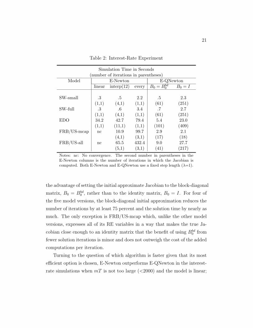
Table 2: Interest-Rate Experiment

Simulation Time in Seconds(number of iterations in parentheses)

Model E-Newton E-QNewtonlinear interp(12) every B0 = Bbd

0 B0 = I

SW-small .3 .5 2.2 .5 2.3(1,1) (4,1) (1,1) (61) (251)

SW-full .3 .6 3.4 .7 2.7(1,1) (4,1) (1,1) (61) (251)

EDO 34.2 42.7 79.4 5.4 23.0(1,1) (11,1) (1,1) (101) (409)

FRB/US-mcap nc 10.9 99.7 2.9 2.1(4,1) (3,1) (17) (18)

FRB/US-all nc 65.5 432.4 9.0 27.7(5,1) (3,1) (41) (217)

Notes: nc: No convergence. The second number in parentheses in theE-Newton columns is the number of iterations in which the Jacobian iscomputed. Both E-Newton and E-QNewton use a fixed step length (λ=1).

the advantage of setting the initial approximate Jacobian to the block-diagonal

matrix, B0 = Bbd0 , rather than to the identity matrix, B0 = I. For four of

the five model versions, the block-diagonal initial approximation reduces the

number of iterations by at least 75 percent and the solution time by nearly as

much. The only exception is FRB/US-mcap which, unlike the other model

versions, expresses all of its RE variables in a way that makes the true Ja-

cobian close enough to an identity matrix that the benefit of using Bbd0 from

fewer solution iterations is minor and does not outweigh the cost of the added

computations per iteration.

Turning to the question of which algorithm is faster given that its most

efficient option is chosen, E-Newton outperforms E-QNewton in the interest-

rate simulations when mT is not too large (<2000) and the model is linear;

22

E-QNewton is faster otherwise. In general, the E-Newton simulations exhibit

much more variation in solution time than do the the E-QNewton simula-

tions. This is clearest in the results for the three linear model versions. In

the simulations with the E-Newton “linear” option, the ratio of the longest

solution time to the shortest solution time is 114; the corresponding ratio

in the simulations with the E-QNewton B0 = Bbd0 option is only 11. This

difference is explained by time required to invert the E-Newton Jacobian,

which varies with the cube of mT . The E-QNewton solution times appear

to be not far from proportional to mT .

The second simulation experiment (table 3) focuses on how well the two

algorithms solve RE models that are substantially nonlinear. For this pur-

pose, a smooth approximation to the constraint that the short-term interest

rate cannot fall below zero is added to each model, and shocks are introduced

that reduce output by an amount sufficient to cause this nonlinearity to have

a large impact on the solution. The magnitude of the shocks is chosen so

that in each model the cumulative loss of output over the first 20 periods is

roughly twice as large as the increase in output that would occur if the signs

of the shocks were reversed. In the simulations, the number of periods that

the rate of interest, if unconstrained, would be less than zero ranges from

seven periods (SW-small and SW-full) to 25 periods (FRB/US-mcap).

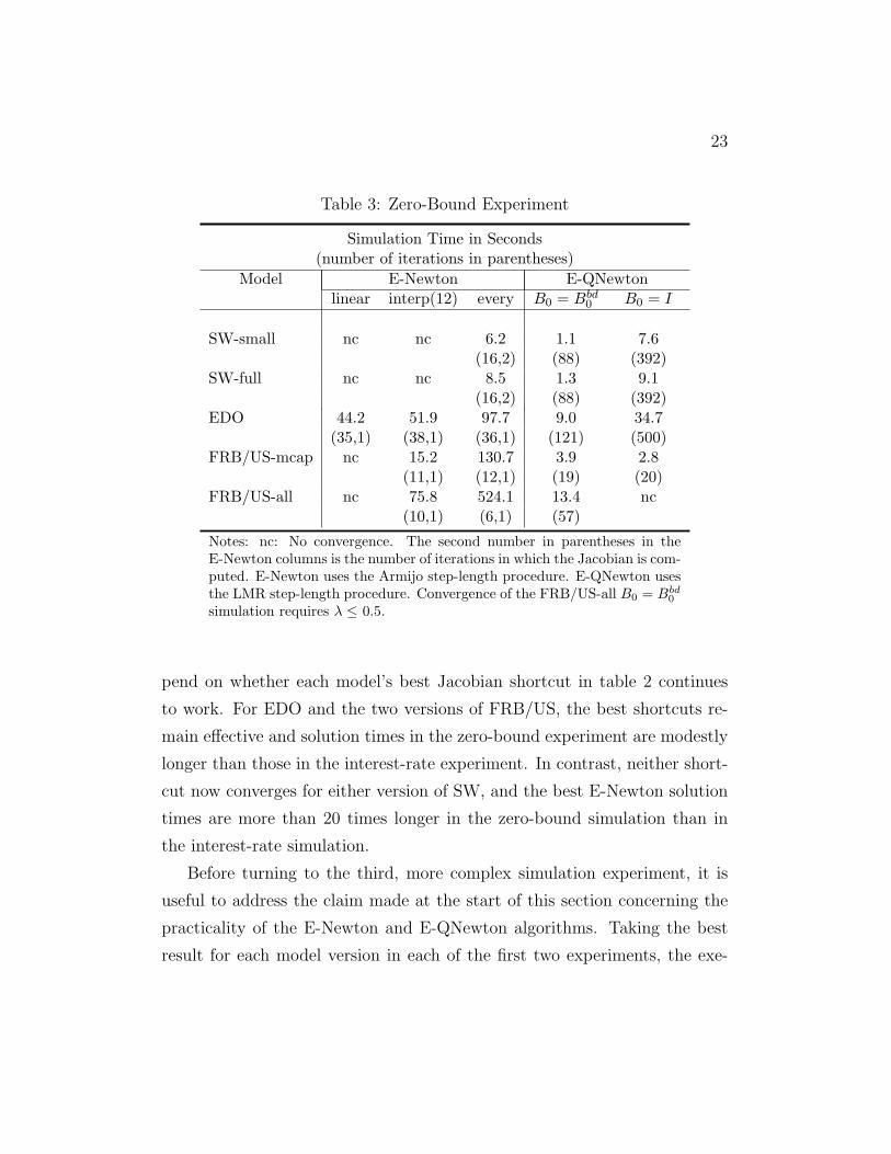
The E-QNewton algorithm completes all of the zero-bound simulations

much more rapidly than does E-Newton. For each model version, the best

E-QNewton solution takes only about 20 percent as long as the best E-Newton

solution. Even though the shocks are not the same, a rough gauge of the

effects on each algorithm of the substantial nonlinearity introduced in this

experiment can be made by comparing the execution times in table 3 with

those in table 2. On this basis, the zero-bound nonlinearity tends to increase

the E-QNewton execution times modestly and relatively uniformly for each

model version. The effects in the E-Newton runs are more variable and de-

23

Table 3: Zero-Bound Experiment

Simulation Time in Seconds(number of iterations in parentheses)

Model E-Newton E-QNewtonlinear interp(12) every B0 = Bbd

0 B0 = I

SW-small nc nc 6.2 1.1 7.6(16,2) (88) (392)

SW-full nc nc 8.5 1.3 9.1(16,2) (88) (392)

EDO 44.2 51.9 97.7 9.0 34.7(35,1) (38,1) (36,1) (121) (500)

FRB/US-mcap nc 15.2 130.7 3.9 2.8(11,1) (12,1) (19) (20)

FRB/US-all nc 75.8 524.1 13.4 nc(10,1) (6,1) (57)

Notes: nc: No convergence. The second number in parentheses in theE-Newton columns is the number of iterations in which the Jacobian is com-puted. E-Newton uses the Armijo step-length procedure. E-QNewton usesthe LMR step-length procedure. Convergence of the FRB/US-all B0 = Bbd

0

simulation requires λ ≤ 0.5.

pend on whether each model’s best Jacobian shortcut in table 2 continues

to work. For EDO and the two versions of FRB/US, the best shortcuts re-

main effective and solution times in the zero-bound experiment are modestly

longer than those in the interest-rate experiment. In contrast, neither short-

cut now converges for either version of SW, and the best E-Newton solution

times are more than 20 times longer in the zero-bound simulation than in

the interest-rate simulation.

Before turning to the third, more complex simulation experiment, it is

useful to address the claim made at the start of this section concerning the

practicality of the E-Newton and E-QNewton algorithms. Taking the best

result for each model version in each of the first two experiments, the exe-

24

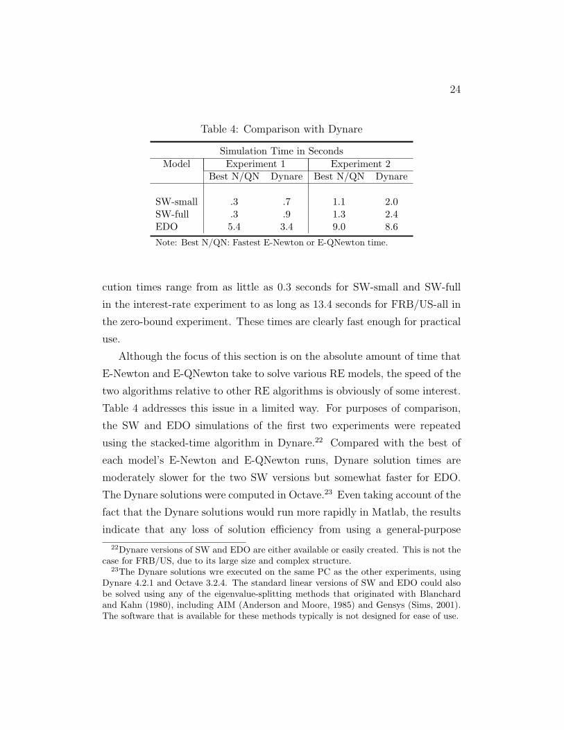
Table 4: Comparison with Dynare

Simulation Time in Seconds

Model Experiment 1 Experiment 2Best N/QN Dynare Best N/QN Dynare

SW-small .3 .7 1.1 2.0SW-full .3 .9 1.3 2.4EDO 5.4 3.4 9.0 8.6

Note: Best N/QN: Fastest E-Newton or E-QNewton time.

cution times range from as little as 0.3 seconds for SW-small and SW-full

in the interest-rate experiment to as long as 13.4 seconds for FRB/US-all in

the zero-bound experiment. These times are clearly fast enough for practical

use.

Although the focus of this section is on the absolute amount of time that

E-Newton and E-QNewton take to solve various RE models, the speed of the

two algorithms relative to other RE algorithms is obviously of some interest.

Table 4 addresses this issue in a limited way. For purposes of comparison,

the SW and EDO simulations of the first two experiments were repeated

using the stacked-time algorithm in Dynare.22 Compared with the best of

each model’s E-Newton and E-QNewton runs, Dynare solution times are

moderately slower for the two SW versions but somewhat faster for EDO.

The Dynare solutions were computed in Octave.23 Even taking account of the

fact that the Dynare solutions would run more rapidly in Matlab, the results

indicate that any loss of solution efficiency from using a general-purpose

22Dynare versions of SW and EDO are either available or easily created. This is not thecase for FRB/US, due to its large size and complex structure.

23The Dynare solutions wre executed on the same PC as the other experiments, usingDynare 4.2.1 and Octave 3.2.4. The standard linear versions of SW and EDO could alsobe solved using any of the eigenvalue-splitting methods that originated with Blanchardand Kahn (1980), including AIM (Anderson and Moore, 1985) and Gensys (Sims, 2001).The software that is available for these methods typically is not designed for ease of use.

25

software platform to run the algorithms described here, rather than using

specialized software designed for RE models, is not that large, and suggest

that for many users this cost may be more than offset by the features available

in the general-purpose environment that facilitate its use.

The final experiment assumes that each model’s monetary policymaker,

rather than following a simple policy rule, sets the short-term rate of interest

to minimize a loss function. For illustrative purposes, the loss function is a

weighted, discounted sum of squared differences of output and inflation from

their baseline values and of the rate of interest from its value in the previous

period. The loss function is minimized over the first 40 simulation periods.

The solution of this experiment requires a sequence of “outer” iterations, each

of which consists of 40 RE derivative solutions that compute the effects on

the arguments of the loss function of perturbations to the policy instrument

in each optimization period, followed by one or more RE solutions in which

the policy variable is set according to these derivatives and the values of the

loss function arguments.

The experiment repeats the output shocks of the second experiment, but

reverses their signs so that output expands initially and the zero bound is

not an issue. Because the Jacobian of a linear model is invariant to where

it is calculated, a single “linear” Jacobian is clearly sufficient to run all of

the necessary E-Newton RE simulations for the linear model versions. In

addition, the optimal-policy solution for these models requires a single outer

iteration. Although FRB/US is nonlinear, the nonlinearity is mild enough

that a single “interp(12)” Jacobian proves to be accurate enough to complete

all of the needed E-Newton RE simulations. The nonlinearity does, however,

increase to three the number of outer iterations needed for convergence to

the optimal-policy solution. That is, the derivatives of the arguments of the

loss function with respect to the policy instrument in each period have to be

computed three times.

26

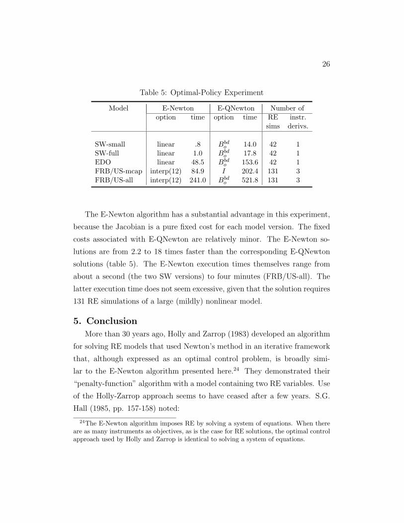
Table 5: Optimal-Policy Experiment

Model E-Newton E-QNewton Number ofoption time option time RE instr.

sims derivs.

SW-small linear .8 Bbdo 14.0 42 1

SW-full linear 1.0 Bbdo 17.8 42 1

EDO linear 48.5 Bbdo 153.6 42 1

FRB/US-mcap interp(12) 84.9 I 202.4 131 3FRB/US-all interp(12) 241.0 Bbd

o 521.8 131 3

The E-Newton algorithm has a substantial advantage in this experiment,

because the Jacobian is a pure fixed cost for each model version. The fixed

costs associated with E-QNewton are relatively minor. The E-Newton so-

lutions are from 2.2 to 18 times faster than the corresponding E-QNewton

solutions (table 5). The E-Newton execution times themselves range from

about a second (the two SW versions) to four minutes (FRB/US-all). The

latter execution time does not seem excessive, given that the solution requires

131 RE simulations of a large (mildly) nonlinear model.

5. Conclusion

More than 30 years ago, Holly and Zarrop (1983) developed an algorithm

for solving RE models that used Newton’s method in an iterative framework

that, although expressed as an optimal control problem, is broadly simi-

lar to the E-Newton algorithm presented here.24 They demonstrated their

“penalty-function” algorithm with a model containing two RE variables. Use

of the Holly-Zarrop approach seems to have ceased after a few years. S.G.

Hall (1985, pp. 157-158) noted:

24The E-Newton algorithm imposes RE by solving a system of equations. When thereare as many instruments as objectives, as is the case for RE solutions, the optimal controlapproach used by Holly and Zarrop is identical to solving a system of equations.

27

The real drawback of [the Holly-Zarrop] technique is . . . that it

severely limits the number of expectations terms that can ap-

pear in the model. Optimal control problems quickly become

intractable as the number of control variables rises and it would

be impossible to use this technique to solve a model with 20 or

more expectations variables.

Later, Fisher (1992, p. 56) concluded:

. . . it is clear that [Holly-Zarrop] methods are not efficient . . .

These observations reflect the limited capabilities of the computer hardware

that was available at the time.

Computer hardware is now cheap by the standards of the past, a devel-

opment that greatly extends the range of RE models for which Newton algo-

rithms like Holly-Zarrop and E-Newton are feasible and practical. Nonethe-

less, if execution speed were the only criteria for comparing solution proce-

dures, neither E-Newton nor E-QNewton would come out on top. Relative to

faster procedures, an important advantage of E-Newton and E-QNewton lies

in their simplicity, which enables them to be coded in software that is easy

to use. This advantage would not have been very important 20 or 30 years

ago, when the time penalty for choosing a user-friendly software product

might have translated into many extra minutes or even hours of execution

time.25 Today, the availability of much faster hardware means that the added

execution time is likely to be measured in seconds and thus less important.

This paper demonstrates the ability of a Newton algorithm that iterates

on a set of expectations estimates to solve several well-known RE models.

25Hollinger (1996) reports solution times using the stacked-time algorithm in Troll forseveral macro models, of which the 466-equation Multimod is closest in size to FRB/US.A 150-period solution of Multimod required 21 minutes on a relatively fast computer.

28

Compared with the Newton procedure developed by Holly and Zarrop, the

E-Newton algorithm presented here contains options that accelerate the com-

putation of the Jacobians of linear and mildly nonlinear RE models.

This paper also develops an RE solution algorithm based on the quasi-

Newton method of Broyden, an approach that appears not to have been

used before on this type of problem. The E-QNewton algorithm combines a

block-diagonal initial estimate of the approximate Jacobian, an economical

approach to updating the approximate Jacobian, and the option to use the

LMR step-length procedure with nonlinear models. E-QNewton solves the

reported single-simulation experiments more rapidly than E-Newton, except

when the model is linear and of small-to-medium size. E-Newton outperforms

E-QNewton on the experiment that involves a set of RE solutions in which

the Newton Jacobian is a one-time fixed cost.

29

Appendix

A.1 Setting up the RE problem

The rational expectations model f(yt−1, yt, yt+1) = 0 is split into two

models, one that has no leads of endogenous variables and one that has no

lags of endogenous variables. The former can be easily solved forward in time

and the latter can be easily solved backward in time.

The model without leads takes the original model and replaces the vector

yt+1 with a vector of expectations estimates, χt, that is based on information

available at t and has two components: the function k(yt−1, yt) of the model’s

endogenous variables and the exogenous vector xt.

f(yt−1, yt, χt) = 0

χt = k(yt−1, yt) + xt

(A1)

The model without lags contains the RE formulas for the expectations es-

timates, whose solutions in the second model are denoted by χ, and the

expectations errors, e.

χt =∑nx

i=1 µiχt+i +∑ny

i=0 νiyt+i

et = χt − χt

(A2)

Note that y is endogenous in (A1) but exogenous in (A2). The pair of models

simplifies to equations 2-3 when the equation for χt in the first model does

not have an endogenous component and the equation for χt in the second

model simplifies to χt = yt+1.

The more general form of A1-A2 is necessary to accomodate two charac-

teristics of the expectations structure of FRB/US that are absent in the other

models. First, the VAR-based expectations framework in FRB/US, although

designed as an alternative to rational expectations, has proved to be a good

starting point for the RE expectations estimates. The VAR-based formulas

30

are the endogenous expectations component in the RE versions of FRB/US.

Second, many FRB/US equations are written in such a way that their ex-

pectations terms correspond to infinite weighted sums of future values of

endogenous variables, not to a single future value. This form appears in the

model’s present value relationships for financial variables and in its decision-

rule representations of some nonfinancial equations. The latter, which are

derived from Euler equations, substitute for one or a few future values of

the dependent variable with infinite future sums of the other variables that

appear in the equation. Because the coefficients of the infinite sums decline

either geometrically or based on a mixture of several geometric parameters,

the sums collapse to the form shown in the lower line of A2. For financial

expectations, the upper summation limits, nx and ny, are one and zero,

respectively. For nonfinancial expectations, the limits are typically greater

than one but never larger than three.

The RE solution of equations A1-A2, which obtains when xt is chosen

such that et = 0 for t = 1, . . . , T , is written compactly as

F (x) = 0. (A3)

The stacked vector of expectations constants, x, has mT elements, where

m is the number of RE variables and T the number of simulation periods.

Convergence to the RE solution occurs at iteration i if the maximum absolute

expectations error, c(x), is less than γc.

c(xi) = max |F (xi)| = max |ei| < γc, (A4)

The ratio of the sum of squared expectations errors in the current and pre-

vious iterations,

g(xi) =e′iei

e′i−1ei−1

, (A5)

31

provides a scalar measure of the progress made toward the RE solution each

iteration.

A.2 The E-Newton algorithm

The organization of the E-Newton algorithm is sketched out below. Ji is

the Jacobian of F at xi, λi is the step length, and di is the step direction.

Parameter values are γj=0.5, γls=0.9, and γc=1e-05.

1. Initialize:

(a) set i = 0; choose y0, yT+1, x0

(b) compute J0

(c) d1 = −J−10 F (x0)

2. For i = 1,maxit

(a) i = i + 1

(b) xi = xi−1 + di

(c) exit if c(xi) < γc

(d) for nonlinear models, invoke Armijo line search if g(xi) > γls

(1) search for satisfactory λi 6= 1

(2) xi = xi−1 + λidi

(3) exit if c(xi) < γc

(e) compute Ji if g(xi) > γj; else Ji = Ji−1

(f) di+1 = −J−1i F (xi)

A.2a The E-Newton Jacobian

The E-Newton RE Jacobian (J), which is an mTxmT matrix, is com-

posed of m2 mxm submatrices.

J =

J11 · · · J1m...

. . ....

Jm1 · · · Jmm

(A6)

32

Submatrix Jjp contains all of the derivatives that involve expectations con-

stant j and expectations error p.

Jjp =

∂ep,1∂xj,1

· · · ∂ep,1∂xj,T

.... . .

...∂ep,T∂xj,1

· · ·∂ep,T∂xj,T

(A7)

The term∂ep,l∂xj,k

denotes the derivative of expectations error p in period l with

respect to expectations constant j in period k.

Impulse-response (IR) simulations are used to calculate the Jacobian.

Each IR simulation, which perturbs a particular xj,k, provides the informa-

tion needed to fill a single column of J . The number of IR simulations

executed each time the Jacobian is calculated depends on the setting of the

“jmeth” option. When “jmeth=every”, all mT IR simulations are run. The

setting “jmeth=linear” runs the 2m IR simulations needed to construct the

Jacobian of a standard, linear RE model. For use with mildly nonlinear mod-

els, the setting “jmeth=interp(r)” computes an approximate Jacobian from

m(p+ 1) IR simulations, where p is the integer part of (T + 1)/r.

The “jmeth=linear” option takes into account the repetitive structure

of the Jacobian of a standard linear RE model. When RE expectations are

based on information at time t for variables at t+1, each Jacobian submatrix

Jjp has the following simple form.

Jjp =

Q(T−1)xT

01x(T−1) φ1x1

(A8)

Q is a matrix in which every element along each diagonal has the same value,

0 is vector of zeros, and φ equals 1.0 if j = p and zero otherwise. The Jacobian

shown in equation 12 is a concrete example of this simple form. Only two

perturbation simulations are needed per RE variable to construct all the

33

Jacobian submatrices. To see this, recall that each simulation fills a matrix

column. Thus, a pair of simulations in which an expectations constant is

separately shocked in periods 1 and T is sufficient to determine all elements

of Q.

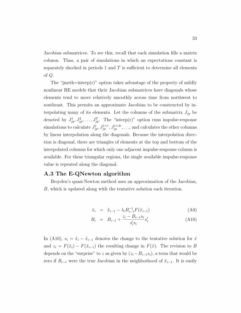
The “jmeth=interp(r)” option takes advantage of the property of mildly

nonlinear RE models that their Jacobian submatrices have diagonals whose

elements tend to move relatively smoothly across time from northwest to

southeast. This permits an approximate Jacobian to be constructed by in-

terpolating many of its elements. Let the columns of the submatrix Jjp be

denoted by J1jp, J

2jp, . . . , J

Tjp. The “interp(r)” option runs impulse-response

simulations to calculate J1jp, J

1+rjp , J1+2r

jp , . . ., and calculates the other columns

by linear interpolation along the diagonals. Because the interpolation direc-

tion is diagonal, there are triangles of elements at the top and bottom of the

interpolated columns for which only one adjacent impulse-response column is

available. For these triangular regions, the single available impulse-response

value is repeated along the diagonal.

A.3 The E-QNewton algorithm

Broyden’s quasi-Newton method uses an approximation of the Jacobian,

B, which is updated along with the tentative solution each iteration.

xi = xi−1 − λiB−1i−1F (xi−1) (A9)

Bi = Bi−1 +zi − Bi−1si

s′isis′i (A10)

In (A10), si = xi − xi−1 denotes the change to the tentative solution for x

and zi = F (xi) − F (xi−1) the resulting change in F (x). The revision to B

depends on the “surprise” to z as given by (zi−Bi−1si), a term that would be

zero if Bi−1 were the true Jacobian in the neighborhood of xi−1. It is easily

34

verified that replacing Bi−1 with the updated Jacobian approximation, Bi,

would have set the ”surprise” to zero.

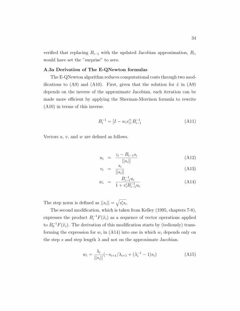
A.3a Derivation of The E-QNewton formulas

The E-QNewton algorithm reduces computational costs through two mod-

ifications to (A9) and (A10). First, given that the solution for x in (A9)

depends on the inverse of the approximate Jacobian, each iteration can be

made more efficient by applying the Sherman-Morrison formula to rewrite

(A10) in terms of this inverse.

B−1i = [I − wiv

′i]B

−1i−1 (A11)

Vectors u, v, and w are defined as follows.

ui =zi −Bi−1si

||si||(A12)

vi =si

||si||(A13)

wi =B−1

i−1ui

1 + v′iB−1i−1ui

(A14)

The step norm is defined as ||si|| =√

s′isi.

The second modification, which is taken from Kelley (1995, chapters 7-8),

expresses the product B−1i F (xi) as a sequence of vector operations applied

to B−10 F (xi). The derivation of this modification starts by (tediously) trans-

forming the expression for wi in (A14) into one in which wi depends only on

the step s and step length λ and not on the approximate Jacobian.

wi =λi

||si||(−si+1/λi+1 + (λ−1

i − 1)si) (A15)

35

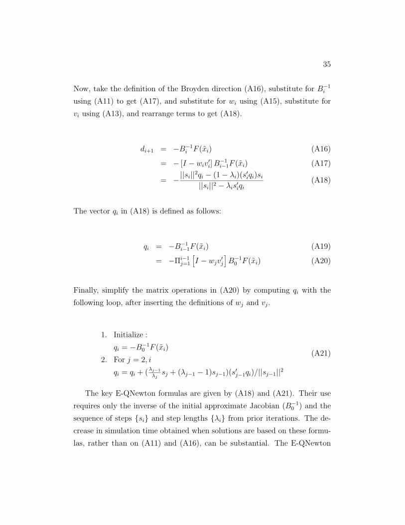
Now, take the definition of the Broyden direction (A16), substitute for B−1i

using (A11) to get (A17), and substitute for wi using (A15), substitute for

vi using (A13), and rearrange terms to get (A18).

di+1 = −B−1i F (xi) (A16)

= − [I − wiv′i]B

−1i−1F (xi) (A17)

= −||si||

2qi − (1− λi)(s′iqi)si

||si||2 − λis′iqi(A18)

The vector qi in (A18) is defined as follows:

qi = −B−1i−1F (xi) (A19)

= −Πi−1j=1

[

I − wjv′j

]

B−10 F (xi) (A20)

Finally, simplify the matrix operations in (A20) by computing qi with the

following loop, after inserting the definitions of wj and vj.

1. Initialize :

qi = −B−10 F (xi)

2. For j = 2, i

qi = qi + (λj−1

λjsj + (λj−1 − 1)sj−1)(s

′j−1qi)/||sj−1||

2

(A21)

The key E-QNewton formulas are given by (A18) and (A21). Their use

requires only the inverse of the initial approximate Jacobian (B−10 ) and the

sequence of steps {si} and step lengths {λi} from prior iterations. The de-

crease in simulation time obtained when solutions are based on these formu-

las, rather than on (A11) and (A16), can be substantial. The E-QNewton

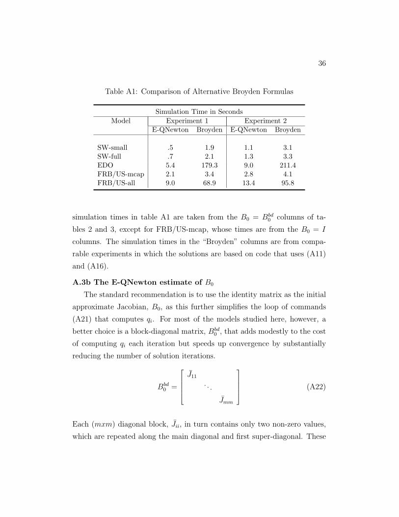
36

Table A1: Comparison of Alternative Broyden Formulas

Simulation Time in Seconds

Model Experiment 1 Experiment 2E-QNewton Broyden E-QNewton Broyden

SW-small .5 1.9 1.1 3.1SW-full .7 2.1 1.3 3.3EDO 5.4 179.3 9.0 211.4FRB/US-mcap 2.1 3.4 2.8 4.1FRB/US-all 9.0 68.9 13.4 95.8

simulation times in table A1 are taken from the B0 = Bbd0 columns of ta-

bles 2 and 3, except for FRB/US-mcap, whose times are from the B0 = I

columns. The simulation times in the “Broyden” columns are from compa-

rable experiments in which the solutions are based on code that uses (A11)

and (A16).

A.3b The E-QNewton estimate of B0

The standard recommendation is to use the identity matrix as the initial

approximate Jacobian, B0, as this further simplifies the loop of commands

(A21) that computes qi. For most of the models studied here, however, a

better choice is a block-diagonal matrix, Bbd0 , that adds modestly to the cost

of computing qi each iteration but speeds up convergence by substantially

reducing the number of solution iterations.

Bbd0 =

J11. . .

Jmm

(A22)

Each (mxm) diagonal block, Jii, in turn contains only two non-zero values,

which are repeated along the main diagonal and first super-diagonal. These

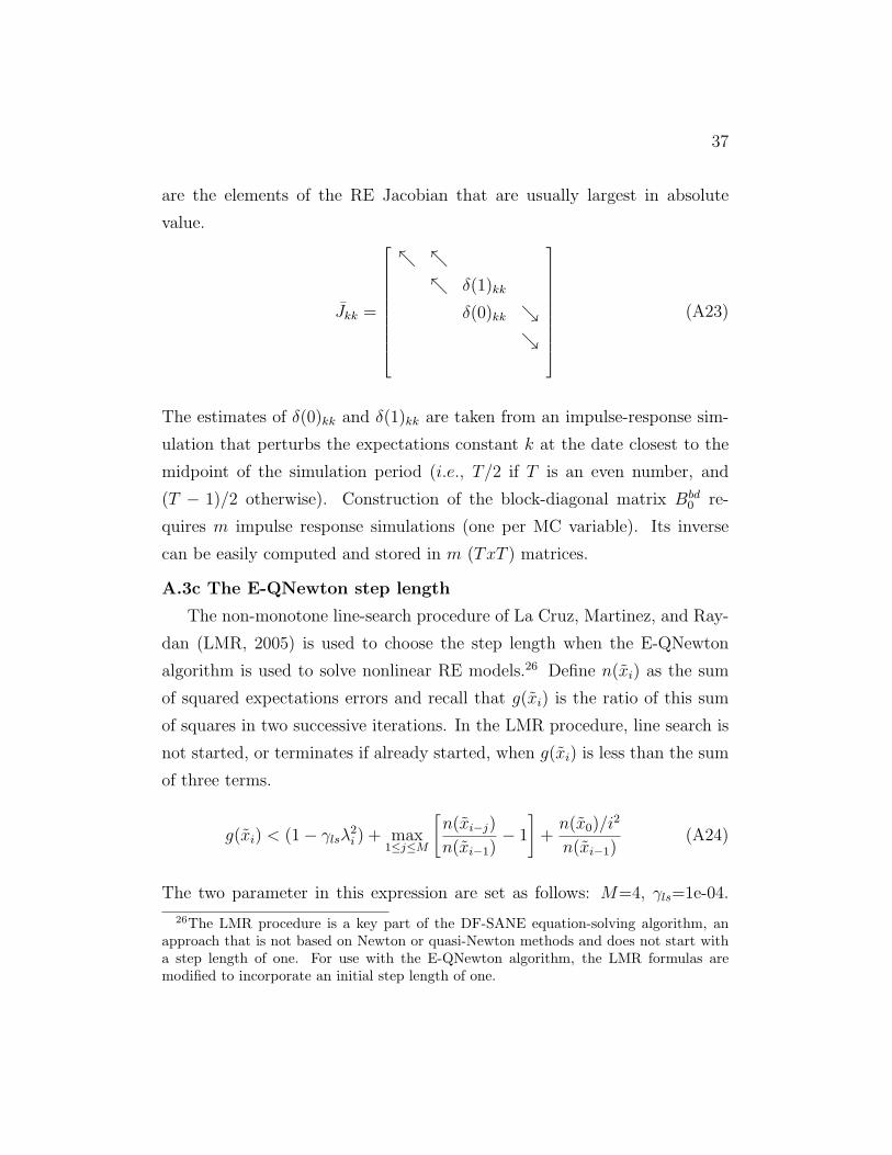
37

are the elements of the RE Jacobian that are usually largest in absolute

value.

Jkk =

տ տ

տ δ(1)kk

δ(0)kk ց

ց

(A23)

The estimates of δ(0)kk and δ(1)kk are taken from an impulse-response sim-

ulation that perturbs the expectations constant k at the date closest to the

midpoint of the simulation period (i.e., T/2 if T is an even number, and

(T − 1)/2 otherwise). Construction of the block-diagonal matrix Bbd0 re-

quires m impulse response simulations (one per MC variable). Its inverse

can be easily computed and stored in m (TxT ) matrices.

A.3c The E-QNewton step length

The non-monotone line-search procedure of La Cruz, Martinez, and Ray-

dan (LMR, 2005) is used to choose the step length when the E-QNewton

algorithm is used to solve nonlinear RE models.26 Define n(xi) as the sum

of squared expectations errors and recall that g(xi) is the ratio of this sum

of squares in two successive iterations. In the LMR procedure, line search is

not started, or terminates if already started, when g(xi) is less than the sum

of three terms.

g(xi) < (1− γlsλ2i ) + max

1≤j≤M

[

n(xi−j)

n(xi−1)− 1

]

+n(x0)/i

2

n(xi−1)(A24)

The two parameter in this expression are set as follows: M=4, γls=1e-04.

26The LMR procedure is a key part of the DF-SANE equation-solving algorithm, anapproach that is not based on Newton or quasi-Newton methods and does not start witha step length of one. For use with the E-QNewton algorithm, the LMR formulas aremodified to incorporate an initial step length of one.

38

The first term on the right hand side of (A24), which is always less than

1.0 at the selected value of γls, by itself leads the procedure to try to find

a step length that reduces the sum of squared expectations errors from one

iteration to the next. The remaining terms act to moderate this requirement.

The second term allows the {n(xi)} sequence to be locally increasing without

invoking line search. The third term, whose value goes to zero in the limit,

prevents rising values of n(xi) from starting line search in the initial iterations

of a solution.

The E-QNewton algorithm starts each iteration with λi = 1 and xi =

di + xi−1. The expression for di is given in (A18). If condition (A24) fails to

hold, the LMR procedure starts and computes a smaller positive step length

(λ+i ).

λ+i =

τminλ+i if αi < τminλ

+i

τmaxλ+i if αi > τmaxλ

+i

αi otherwise

(A25)

where

αi =λ+2

i n(xi−1)

n(xi−1 + λ+i di) + (2λ+

i − 1)n(xi−1)(A26)

When λ+i appears on the right hand side of either (A25) or (A26), it denotes

the value that was assigned to that parameter prior to the current step-length

iteration, which is 1.0 initially. If condition (A24) is satisfied at the new value

of λ+i , line search terminates. If the condition is not satisfied, a negative step

length (λ−i ) is computed using a set of analogous formulas. In this case, the

value of λ−i that appears on the right hand side of the formulas is initially

set to -1.0. If condition (A24) is satisfied at the new value of λ−i , line search

terminates. If the condition is not satisfied, line search continues with ever

smaller values of λ+i and λ−

i until the condition is satisfied or the maximum

39

number of line-search iterations is reached. The simulation experiments set

τmax=.5 and τmin=.1.

40

References

Armstrong, John, Richard Black, Douglas Laxton, and David Rose, 1998. “ARobust Method for Simulating Forward-Looking Models,” Journal of Eco-

nomic Dynamics and Control, 22, 489-501.

Anderson, Gary and George Moore. 1985, “A Linear Algebraic Procedure forSolving Linear Perfect Foresight Models,” Economics Letters, 17, 247-252.

Blanchard, Olivier and Charles Kahn. 1980, “The Solution of Linear Differ-ence Models Under Rational Expectations,” Econometrica, 48: 1305-1311.

Broyden, C.G. 1965, “A Class of Methods for Solving Nonlinear SimultaneousEquations,” Mathematics of Computation, 19: 577-593.

Brayton, Flint, Andrew Levin, Ralph Tryon, and John C. Williams. 1997a,“The Evolution of Macro Models at the Federal Reserve Board,” Carnegie-

Rochester Conference Series on Public Policy, 47: 43-81.

Brayton, Flint, Eileen Mauskopf, Dave Reifschneider, Peter Tinsley, andJohn Williams. 1997b, “The Role of Expectations in the FRB/US Macroe-conomic Model,” Federal Reserve Bulletin, April: 227-245.(http://www.federalreserve.gov/pubs/bulletin/1997/199704lead.pdf)

Brayton, Flint and Peter Tinsley. 1996, “A Guide to FRB/US: A Macroe-conomic Model of the United States,” Finance and Economics DiscussionSeries 1996-42, Federal Reserve Board, Washington, DC.(http://www.federalreserve.gov/pubs/feds/1996/199642/199642pap.pdf)

Chung, Hess, Michael Kiley, and Jean-Phillipe Laforte. 2010, “Documenta-tion of the Estimated, Dynamic, Optimization-Based (EDO) Model of theU.S. Economy: 2010 Version,” Finance and Economics Discussion Series2010-29, Federal Reserve Board, Washington, DC.(http://www.federalreserve.gov/pubs/feds/2010/201029/201029pap.pdf)

Edge, Rochelle, Michael Kiley and Jean-Phillipe Laforte. 2008, “An Esti-mated DSGE Model of the U.S. Economy with an Application to NaturalRate Measures,” Journal of Economic Dynamics and Control, 32(8): 2512-2535.

41

Fair, Ray and John Taylor. 1983, “Solution and Maximum Likelihood Es-timation of Dynamic Rational Expectations Models,” Econometrica, 51(4):1169-1185.

Fisher, Paul. 1992, Rational Expectations in Macroeconomic Models, KluwerAcademic Publishers, London.

Fisher, P.G. and A.J. Hughes Hallett. 1988, “Efficient Solution Techniquesfor Linear and Non-Linear Rational Expectations Models,” Journal of Eco-

nomic Dynamics and Control, 12: 635-657.

Gay, David. 1979, “Some Convergence Properties of Broyden’s Method,”SIAM Journal of Numerical Analysis, 16: 623-630.

Hall, S.G. 1985, “On the Solution of Large Economic Models with ConsistentExpectations,” Bulletin of Economic Research, 37: 157-161.

Hollinger, Peter. 1996, “The Stacked-Time Simulator in TROLL: A RobustAlgorithm for Solving Forward-Looking Models,” Second International Con-ference on Computing in Economics and Finance, Society of ComputationalEconomics. (http://www.unige.ch/ce/ce96/ps/hollinge.eps)

Holly, S. and M.B. Zarrop. 1983, “On Optimality and Time ConsistencyWhen Expectations are Rational,” European Economic Review, 20: 23-40.

Juillard, Michel. 1996, “DYNARE: A Program for the Resolution and Simu-lation of Dynamic Models with Forward Variables Through the Use of a Re-laxation Algorithm,” CEPREMAP Working Paper no. 9602, Paris, France.

Juillard, Michel, Douglas Laxton, Peter McAdam, and Hope Pioro. 1999,“Solution Methods and Non-Linear Forward-Looking Models,” in Analyses in

Macroeconomic Modelling, eds., Andrew Hughes Hallett and Peter McAdam,Kluwer.

Kelley, C.T. 1995, Iterative Methods for Linear and Nonlinear Equations,SIAM Publications, Philadelphia.

La Cruz, W., J.M. Martinez, and M. Raydan. 2005, “Spectral ResidualMethod Without Gradient Information for Solving Large-Scale NonlinearSystems of Equations,” Mathematics of Computation, 75: 1429-1448.

42

Sims, Christopher. 2001, “Solving Linear Rational Expectations Models,”Computational Economics, 20: 1-20.

Smets, Frank and Rafael Wouters. 2007, “Shocks and Frictions in US Busi-ness Cycles: A Bayesian DSGE Approach,” American Economic Review,97(3): 586-606.