Embed Size (px)
Citation preview
A Minor Project
on
Analysis of Mechanical Vibration in spring mass damper model and
Machining Processes A report submitted in partial fulfillment to the degree of
Bachelor of Technology
in
Mechanical Engineering
Submitted by
Ankur Shukla (2K12/ME/044)
Ankur Gupta (2K12/ME/043)
Aman Handa (2K12/ME/028)
Under the supervision of
Dr. R. C. Singh Shri Roop Lal
Mechanical Engineering Department,
Delhi Technological University, Delhi
Delhi Technological University
CERTIFICATE
This is to certify that the thesis entitled, “Analysis of mechanical
vibrations in machining processes” submitted by Ankur Shukla, Ankur Gupta
and Aman Handa in partial fulfillment of the requirement for the award
of Bachelor of Technology degree in Mechanical Engineering at Delhi
Technological University, Delhi is an authentic work carried out by them
under my supervision and guidance. To the best of my knowledge, the
matter embodied in the thesis has not been submitted to any other
University/Institute for the award of any Degree or Diploma.
Dr. R.C. Singh Shri. Roop Lal
Department of Mechanical Engineering Department of Mechanical Engineering
Delhi Technological University, Delhi Delhi Technological University, Delhi

ACKNOWLEDGEMENT
I wish to express my profound gratitude and indebtedness to Dr.
R.C. Singh and Shri Rooplal sir, Department of Mechanical
Engineering , Delhi Technological University, Delhi for introducing the present
topic and for their inspiring guidance , constructive criticism and
valuable suggestion throughout the project work. Last but not least,
my sincere thanks to all our friends who have patiently extended
all sorts of help for accomplishing this undertaking.
Ankur Shukla (2K12/ME/044)
Ankur Gupta (2K12/ME/043)
Aman Handa (2K12/ME/028)
Dept. of Mechanical Engineering,
DTU, Delhi-110042

Abstract
Vibration is a mechanical phenomenon in which oscillations occur about an equilibrium point. The
oscillations may be periodic such as the motion of a pendulum. In most of the engineering
applications, vibration is signifying to and fro motion, which is undesirable. In this study, we have
analyzed the basic form of vibration around the simple spring mass damper model. Both type of
vibration i.e. free and forced has been studied by us and typical time response is presented in this
study. Time response is a graphical representation of displacement produced by vibrations with
respect to change in time. We have represented time response based on previous differential equation
established for different type of vibration with and without damping. In this study, we have included
our experimentation results and results are compared with the results obtained using MATLAB to
plot the modal natural frequency curve. Module frequencies can be highly useful for vibrational
analysis and the resonance in structure.
More often, vibration is undesirable, wasting energy and creating unwanted sound – noise. So it is
necessary to isolate vibration from the machine parts. For isolating vibration, first we have to analyze
the vibration in the part. In this study we have represented a vibration analyzer which is able to
analyze the chatter vibration in the machining processes and parts and represent it in an easy to
understand form.
Chatter vibrations are present in almost all machining operations and they are major obstacles in
achieving desired productivity. The objective of this study to analyze the different type of vibration
in machining processes by presented vibration analyzer.

1 | M i n o r P r o j e c t R e p o r t
Contents
Title Page No.
Certificate (i)
Acknowledgement (ii)
Abstract (iii)
List of figures 2
Chapter 1 Introduction 3
1.1 Types of Vibration 4
1.2 Scope and objective of Work 6 Chapter 2 Literature review 7
Chapter 3 Numerical Formulation 10
3.1 Free vibration without damping 11
3.1.1 Vibration of a system from conservation of energy point of view 12
3.2 Free vibration with damping 12
3.3 Forced vibration without damping 14
3.4 Forced vibration with damping 16
3.4.1 Velocity and Acceleration Response 18
3.4.2 Resonance Frequencies 18
3.5 Two degree of freedom: Vibrations 19
3.5.1 System of three springs and two masses 19
3.6 Multiple degree of freedom: Vibrations 24
Chapter 4 Matlab Modeling 27
4.1 Simscape Model 28
4.2 Simulink Model 29
Chapter 5 Vibrational analyser 30
Chapter 6 Results 32
Chapter 7 Conclusion 42
References 44
Appendix 1 46

2 | M i n o r P r o j e c t R e p o r t
List of figures
Figure 1 Spring Mass Damper Model for free vibration Source: [16] ............................................................................. 11
Figure 2 Spring Mass Damper model for free vibration with damping Source : [16] ......................................................12
Figure 3 Spring Mass Damper model for Forced Vibration Source: [17] ........................................................................15
Figure 4 Spring Mass Damper model for Forced vibration with damping Source : [17] ..................................................16
Figure 5 Spring Mass Damper model for System of three springs and two masses Source : [17] ....................................19
Figure 6 Spring Mass Damper model for system of three springs and two masses with dampers Source : [16]................24
Figure 7 Simscape model of spring mass damper system ...............................................................................................28
Figure 8 Simulink model of Spring Mass Damper Vibration ..........................................................................................29
Figure 9 Displacement-Time Response of Free Vibration : Undamped ..........................................................................33
Figure 10 Velocity-Time Responce of Free Vibration: Undamped ...............................................................................34
Figure 11 Velocity-Time Responce of damped Free Vibration: Critically Damped .........................................................34
Figure 12 Displacement-Time Response of damped Free Vibration: Critically Damped .................................................35
Figure 13Velocity-Time Response of damped Free Vibration: Under Damped ...............................................................35
Figure 14 Displacement-Time Responce of damped Free Vibration: Under Damped ......................................................36
Figure 15 Displacement-Time Response of damped Free Vibration: Over Damped ........................................................36
Figure 16 Velocity-Time Response of damped Free Vibration: Over Damped ................................................................37
Figure 17 Displacement-Time Response of Forced Vibration: Undamped ......................................................................37
Figure 18 Velocity-Time Response Of Forced Vibration: Undamped .............................................................................38
Figure 19 Displacement-Time Response of damped Forced Vibration: Critically Damped .............................................38
Figure 20 Velocity-Time Response of damped Forced Vibration: Critically Damped ......................................................39
Figure 21 Displacement-Time Response of damped Forced Vibration: Over Damped ....................................................39
Figure 22 Velocity -Time Response of damped Forced Vibration: Over Damped ...........................................................40
Figure 23 Displacement-Time Response of damped Forced Vibration: Under Damped ..................................................40
Figure 24 Velocity -Time Response of damped Forced Vibration: Under Damped..........................................................41
3 | M i n o r P r o j e c t R e p o r t
cHApTer: 1
4 | M i n o r P r o j e c t R e p o r t
1. Introduction Vibration is signifying to and fro motion, which is undesirable. Galileo discovered the relationship
between the length of a pendulum and its frequency and observed the resonance of two bodies that
were connected by some energy transfer medium and tuned to the same natural frequency. Vibration
may results in the failure of machines or their critical components. The effect of vibration depends on
the magnitude in terms of displacement, velocity or accelerations, exciting frequency and the total
duration of the vibration. In this study, the vibration of a single -degree-of-freedom (SDOF), Two
degree of freedom system with and without damping.
Vibration is a mechanical phenomenon whereby oscillations occur about an equilibrium point. The
oscillations may be periodic such as the motion of a pendulum or random such as the movement of a
tire on a gravel road [16].
Vibration is undesirable, wasting energy and creating unwanted sound – noise. For example, the
vibrational motions of engines, electric motors, or any mechanical device in operation are typically
unwanted. Such vibrations can be caused by imbalances in the rotating parts, uneven friction, the
meshing of gear teeth, etc. Careful designs usually minimize unwanted vibrations [17].
In basic mechanics, we study single degree-of-freedom systems thoroughly. One might wonder why
so much attention should be given to such a simple problem. The single degree-of-freedom system is
so interesting to study because it gives us information on how a system’s characteristics are
influenced by different quantities. Moreover, one can model more complex systems, provided that
they have isolated resonances, as sums of simple single degree-of-freedom systems. So first we
studied about single degree of freedom vibration of every type. Then we formulate the differential
equation for two and multiple degree of freedom vibrations. We analyzed every situation by Matlab
program and plotted modal natural frequency curve.
1.1 Types of Vibration
Free vibration occurs when a mechanical system is set off with an initial input and then allowed to
vibrate freely. Examples of this type of vibration are pulling a child back on a swing and then letting
go or hitting a tuning fork and letting it ring. The mechanical system will then vibrate at one or more
of its "natural frequency" and damp down to zero [16].
Forced vibration is when a time-varying disturbance (load, displacement or velocity) is applied to a
mechanical system. The disturbance can be a periodic, steady-state input, a transient input, or a
random input. The periodic input can be a harmonic or a non-harmonic disturbance [16]. Examples
of these types of vibration include a shaking washing machine due to an imbalance, transportation
vibration (caused by truck engine, springs, road, etc.), or the vibration of a building during an
earthquake. For linear systems, the frequency of the steady-state vibration response resulting from
the application of a periodic, harmonic input is equal to the frequency of the applied force or motion,
with the response magnitude being dependent on the actual mechanical system.

5 | M i n o r P r o j e c t R e p o r t
Damping is an influence within or upon an oscillatory system that has the effect of reducing,
restricting or preventing its oscillations. In physical systems, damping is produced by processes that
dissipate the energy stored in the oscillation. Examples include viscous drag in mechanical systems,
resistance in electronic oscillators, and absorption and scattering of light in optical oscillators.
Damping not based on energy loss can be important in other oscillating systems such as those that
occur in biological systems [16].
The damping of a system can be described as being one of the following:
• Overdamped: The system returns (exponentially decays) to equilibrium without
oscillating.
• Critically damped: The system returns to equilibrium as quickly as possible without
oscillating.
• Underdamped: The system oscillates (at reduced frequency compared to the undamped case
with the amplitude gradually decreasing to zero.
• Undamped: The system oscillates at its natural resonant frequency (ωo).
For example, consider a door that uses a spring to close the door once open. This can lead to any of
the above types of damping depending on the strength of the damping. If the door is undamped it
will swing back and forth forever at a particular resonant frequency. If it is underdamped it will
swing back and forth with decreasing size of the swing until it comes to a stop. If it is critically
damped then it will return to closed as quickly as possible without oscillating. Finally, if it is
overdamped it will return to closed without oscillating but more slowly depending on how
overdamped it is. Different levels of damping are desired for different types of systems [16].
Metal cutting processes can entail three different types of mechanical vibrations that arise due to the
lack of dynamic stiffness of one or several elements of the system composed by the machine tool, the
tool holder, the cutting tool and the work piece material. These three types of vibrations are known
as free vibrations, forced vibrations and self-excited vibrations[1].
Free vibrations occur when the mechanical system is displaced from its equilibrium and is allowed to
vibrate freely. In a metal removal operation, free vibrations appear, for example, as a result of an
incorrect tool path definition that leads to a collision between the cutting tool and the workpiece.
Forced vibrations appear due to external harmonic excitations [2].. The principal source of forced
vibrations in milling processes is when the cutting edge enters and exits the workpiece. However,
forced vibrations are also associated, for example, with unbalanced bearings or cutting tools, or it can
be transmitted by other machine tools through the workshop floor. Free and forced vibrations can be
avoided, reduced or eliminated when the cause of the vibration is identified. Engineers have
developed several widely known methods to mitigate and reduce their occurrence. Self-excited
vibrations extract energy to start and grow from the interaction between the cutting tool and the

6 | M i n o r P r o j e c t R e p o r t
workpiece during the machining process. This type of vibration brings the system to instability and is
the most undesirable and the least controllable. For this reason, chatter has been a popular topic for
academic and industrial research [2].
1.3 Objective and Scope of work
In this study we analyzed very basic form of vibrations such as free, forced vibration with and
without damping. We have included our experimentation results and these results are compared with
results obtained via MATLAB, to plot the model natural frequency curve. In this study we have
represented a vibration analyser, which is able to analyse the chatter vibration in machining
processes and machine parts and represent it in an easy and understandable form. The objective to
conduct this study is to analyse the different type of vibration in machining processes by presented
vibration analyser.

7 | M i n o r P r o j e c t R e p o r t
cHApTer: 2

8 | M i n o r P r o j e c t R e p o r t
2. Literature Review
Vibration can be regarded as a branch of dynamics that deals with periodic and oscillatory motion.
Common example of vibration problems are the response of civil engineering structures to dynamic
loading, ambient condition and earthquakes, vibration of the unbalanced rotating machines and
vibration of power line due to wind excitations, and aircraft wings [11].
Usually, vibrations are due to elastic forces. Whenever a body is displaced from its equilibrium
position, work is done on the elastic constraint of the forces on the body and is stored as a strain
energy. Now, if body is released, the internal forces cause the body to move towards its equilibrium
position. If the motion is frictionless the strain energy stored in the body is converted into kinetic
energy during the period the body reaches the equilibrium position at which it has maximum kinetic
energy. The body passes through the mean position, the kinetic energy is utilized to overcome the
elastic forces and is stored in the form of strain energy, and so on [12] . For mathematical analysis of
a vibratory system, it is necessary to have a idealized model of the same which appropriately
represent the system [12]. The spring mass damper system is the idealized model for the vibration
analysis.
Vibrations are produced in machine having unbalanced masses. These vibrations will be transmitted
to the foundation upon which the machine is installed. This is usually undesirable. To diminish the
transmitted vibration, machines are usually mounted on spring or dampers, or on some other
vibration isolating material [12].
Jiao Chunwang, Liu Jie, Guo Dameng and Wang Qianqian [10] studied that It is of paramount
importance to acquire the response of many nonlinear forced vibration system. They developed a
new method to explore the approximate analytical solution of forced vibration system which is
named harmonic iteration method (HIM).
Phani Srikantha A., Woodhouse J. [9] studied parametric identification of viscous damping models
in the context of linear vibration theory. Frequency domain identification methods based on
measured frequency response functions (FRFs) are considered.
Vibrations in machining result from the lack of dynamic stiffness of some component of the machine
tool-tool holder cutting tool-work piece system. They can be divided into free, forced and
self-excited vibrations. If the system is well balanced, the second type of vibration is due to variable
chip thickness and the interrupted nature of the process. That means that they are always present.
Therefore, to prevent damage, the vibration level must be controlled. The most common self-excited
vibration is regenerative chatter [2].
Hao Jiang, Xinhua Long, and Guang Meng [13] said Cutting vibration is unavoidable during a
machining process and has great impact on the machined surface. With the increase of the demand
on the high quality of surface finish, the effects of cutting vibration on surface generation attract a lot
of attentions.
A great deal of research has been carried out on the chatter problem since the late 1950s, when
Tobias and Fishwick [3], Tlusty and Polacek [6]and Merrit [7] presented the first research results
focused on this phenomenon. Lots of significant advances have been made over the years. Advances
in computers, sensors and actuators have increased understanding of the phenomena, and developed
and improved strategies to solve the problem [2].
The advantages of detecting, identifying, avoiding, preventing, reducing, controlling or suppressing

9 | M i n o r P r o j e c t R e p o r t
chatter are obvious from the negative effects avoided: poor surface quality, unacceptable inaccuracy,
excessive noise and tool wear, machine tool damage, reduced material removal rate (MRR),
increased costs in terms of time, materials and energy, environmental impact and costs of recycling,
reprocessing or dumping non-valid final parts to recycling points [2].
Chatter vibrations are present in almost all cutting operations and they are major obstacles in
achieving desired productivity. Regenerative chatter is the most detrimental to any process as it
creates excessive vibration between the tool and the work piece, resulting in a poor surface finish,
high-pitch noise and accelerated tool wear which in turn reduces machine tool life, reliability and
safety of the machining operation [4].
Chatter was first identified as a limitation of machining productivity by Taylor [5], who carried out
extensive studies on metal cutting processes as early as in the 1800s. A 3/4 power law cutting force
model was derived and it was stated that chatter is the ‘‘most obscure and delicate of all problems
facing the machinist’’ [4].
Quintana and Ciurana [2] recently presented a state-of-the-art review of chatter in machining
processes and classified current methods which ensure chatter-free (stable) cutting conditions. The
process of chatter analysis, chatter stability prediction and chatter detection is highly complex which
needs to be investigated independently for different cutting processes like turning, milling and
drilling. The literature available till date on each of these processes is tremendous and it provides
motivation to the authors of this paper to produce a state-of-the-art review focusing on the turning
process alone.
When machining high precision mechanical parts, self-excited chatter vibrations must be absolutely
avoided since they cause unacceptable surface finish and dimensional errors. Such unstable
vibrational phenomena typically arise when the overall machining system stiffness is relatively low,
as in the case of internal turning operations performed with slender boring bars [8].
When machining high-precision mechanical components, the static and dynamic behavior of the
machining system during the cutting process plays a fundamental role, since it greatly affects the
obtained surface quality. Basically, machining system vibrations can be split into the sum of forced
and chatter vibrations. Forced vibrations are generated during a regular cutting process and they
cannot be completely avoided due to the compliance of the machining system [8].

10 | M i n o r P r o j e c t R e p o r t
cHApTer: 3

11 | M i n o r P r o j e c t R e p o r t
3. NUMERICAL FORMULATION
3.1 FREE VIBRATION WITHOUT DAMPING
Figure 1 Spring Mass Damper Model for free vibration Source: [16]
To start the investigation of the mass–spring–damper assumes the damping is negligible and that
there is no external force applied to the mass (i.e. free vibration). Most of the system exhibit simple
harmonic motion or oscillation. These systems are said to have elastic restoring forces. Such systems
can be modeled, in some situations, by a spring-mass schematic, as illustrated in Figure. This
constitutes the most basic vibration model of a machine structure and can be used successfully to de
scribe a surprising number of devices, machines, and structures. This system provides a simple
mathematical model that seems to be more sophisticated than the problem requires. This system is
very useful to conceptualize the vibration problem in different machine components.
The force applied to the mass by the spring is proportional to the amount the spring is stretched "x"
(we will assume the spring is already compressed due to the weight of the mass). The proportionality
constant, k, is the stiffness of the spring and has units of force/distance (e.g. lbf/in or N/m). The
negative sign indicates that the force is always opposing the motion of the mass attached to it:
Fs = -kx (3.1) The force generated by the mass is proportional to the acceleration of the mass as given by Newton’s
second law of motion :
∑ � = �� = �ẍ = ��2���2
The sum of the forces on the mass then generates this ordinary differential equation:
�ẍ + �� = 0 (3.2) Assuming that the initiation of vibration begins by stretching the spring by the distance of A and
releasing, the form of the solution of previous equation is found from substitution of an assumed
periodic motion as,
12 | M i n o r P r o j e c t R e p o r t
x(t) = A sin(ω t + ϕ) (3.3)
Where, ω = k/m is the natural frequency (rad/s), A= the amplitude Φ= phase shift,
A and Φ are constants of integration determined by the initial conditions.
If x0 is the specified initial displacement from equilibrium of mass m, and v0 is its specified initial
velocity, simple substitution allows the constants A and Φ to be obtained. The unique displacement
may be expressed as,
x(t) =��
ꙍ� sin ꙍnt+ x0cos ꙍnt (3.4)
3.1.1 Vibration of a system from conservation of energy point of view
Vibrational motion could be understood in terms of conservation of energy. In the above example the
spring has been extended by a value of x and therefore some potential energy (�
����) is stored in the
spring. Once released, the spring tends to return to its un-stretched state (which is the minimum
potential energy state) and in the process accelerates the mass. At the point where the spring has
reached its un-stretched state all the potential energy that we supplied by stretching it has been
transformed into kinetic energy (�
����) [16].
The mass then begins to decelerate because it is now compressing the spring and in the process
transferring the kinetic energy back to its potential. Thus oscillation of the spring amounts to the
transferring back and forth of the kinetic energy into potential energy. In this simple model the mass
will continue to oscillate forever at the same magnitude, but in a real system there is always damping
that dissipates the energy, eventually bringing it to rest [16].
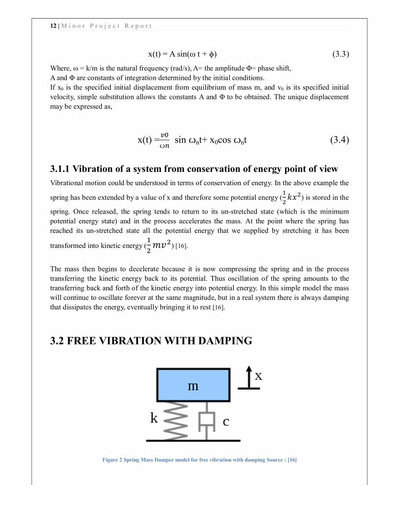
3.2 FREE VIBRATION WITH DAMPING
Figure 2 Spring Mass Damper model for free vibration with damping Source : [16]
13 | M i n o r P r o j e c t R e p o r t
When a "viscous" damper is added to the model that outputs a force that is proportional to the
velocity of the mass. The damping is called viscous because it models the effects of a fluid within an
object. The proportionality constant c is called the damping coefficient and has units of Force over
velocity (lbf s/ in or N s/m).
�� = −�� = −�ẋ = −���
�� (3.5)
Summing the forces on the mass results in the following ordinary differential equation:
�ẍ + �ẋ + �� = 0 (3.6)
The solution to this equation depends on the amount of damping. If the damping is small enough the
system will still vibrate, but eventually, over time, will stop vibrating. This case is called
underdamping – this case is of most interest in vibration analysis. If the damping is increased just to
the point where the system no longer oscillates the point of critical damping is reached (if the
damping is increased past critical damping the system is called overdamped). The value that the
damping coefficient needs to reach for critical damping in the mass spring damper model is:
C� = 2√�� (3.7)
To characterize the amount of damping in a system a ratio called the damping ratio (also known as
damping factor and % critical damping) is used. This damping ratio is just a ratio of the actual
damping over the amount of damping required to reach critical damping. The formula for the
damping ratio (ξ) of the mass spring damper model is:
� =�
�√�� (3.8)
For example, metal structures (e.g. airplane fuselage, engine crankshaft) will have damping factors
less than 0.05 while automotive suspensions in the range of 0.2–0.3.
The solution to the underdamped system for the mass spring damper model is the following:
�(�) = ����ꙍ� cos(�1 − ��ꙍ� − �]), (3.9)
Where ꙍ� = 2� ��
The value of X, the initial magnitude, and Φ the phase shift, are determined by the amount the spring
is stretched. The formulas for these values can be found in the references.
Damped and undamped natural frequencies:
14 | M i n o r P r o j e c t R e p o r t
The major points to note from the solution are the exponential term and the cosine function. The
exponential term defines how quickly the system “damps” down – the larger the damping ratio, the
quicker it damps to zero. The cosine function is the oscillating portion of the solution, but the
frequency of the oscillations is different from the undamped case.
The frequency in this case is called the "damped natural frequency", �� and is related to the
undamped natural frequency by the following formula:
�� = ���1 − �� (3.10)
The damped natural frequency is less than the undamped natural frequency, but for many practical
cases the damping ratio is relatively small and hence the difference is negligible. Therefore the
damped and undamped description are often dropped when stating the natural frequency (e.g. with
0.1 damping ratio, the damped natural frequency is only 1% less than the undamped) [16].
3.3 FORCED VIBRATION WITHOUT DAMPING
Force Applied to Mass. When the sinusoidal force F = F0 sin ωt is applied to the mass of the
undamped single degree of-freedom system , the differential equation of motion is
m�̈ + k� =��sinωt (3.11)
The solution of this equation is
� = A sin ��t + B cos ��t + ��/�
��� �/� �� sin ωt (3.12)
15 | M i n o r P r o j e c t R e p o r t
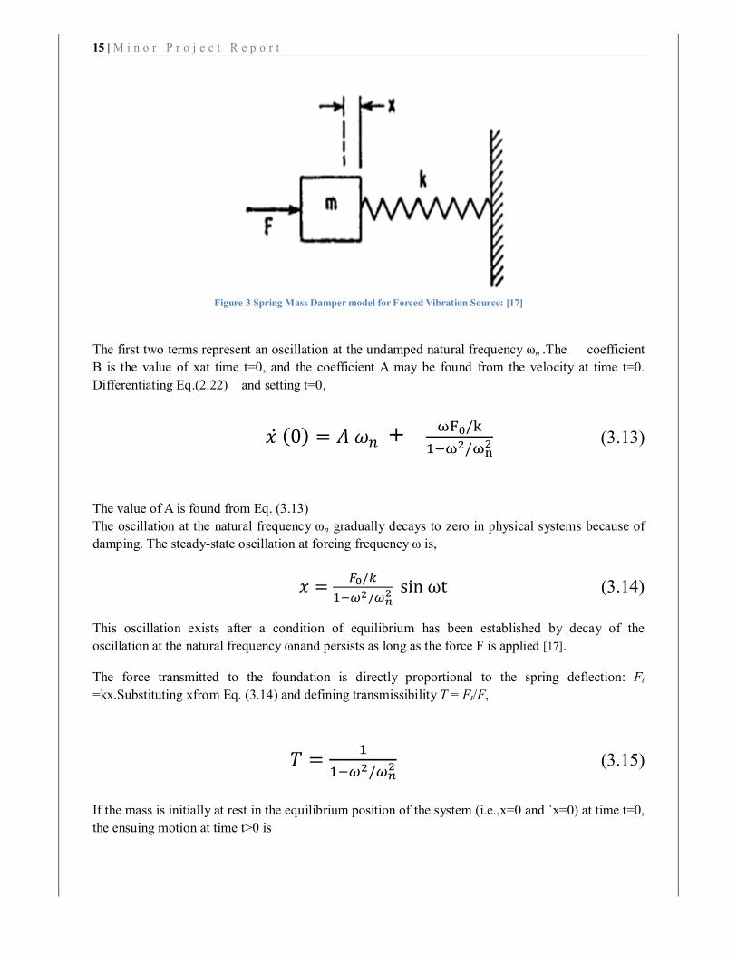
Figure 3 Spring Mass Damper model for Forced Vibration Source: [17]
The first two terms represent an oscillation at the undamped natural frequency ωn .The coefficient
B is the value of xat time t=0, and the coefficient A may be found from the velocity at time t=0.
Differentiating Eq.(2.22) and setting t=0,
� ̇ (0) = � �� + ���/�
����/��� (3.13)
The value of A is found from Eq. (3.13)
The oscillation at the natural frequency ωn gradually decays to zero in physical systems because of
damping. The steady-state oscillation at forcing frequency ω is,
� =��/�
��� �/� �� sin ωt (3.14)
This oscillation exists after a condition of equilibrium has been established by decay of the
oscillation at the natural frequency ωnand persists as long as the force F is applied [17].
The force transmitted to the foundation is directly proportional to the spring deflection: Ft
=kx.Substituting xfrom Eq. (3.14) and defining transmissibility T = Ft/F,
� =�
��� �/� �� (3.15)
If the mass is initially at rest in the equilibrium position of the system (i.e.,x=0 and ˙x=0) at time t=0,
the ensuing motion at time t>0 is

16 | M i n o r P r o j e c t R e p o r t
� =���
����
���
(sin ωt −�
� � sin �� t) (3.16)
For large values of time, the second term disappears because of the damping inherent in any physical
system, and Eq. (3.16) becomes identical to Eq. (3.14).
When the forcing frequency coincides with the natural frequency,ω= ωn and a condition of resonance
exists. Then Eq. (3.16) is indeterminate and the expression for x may be written as
� = −���
�� � ����� +
��
������� (3.17)
According to Eq. (3.17), the amplitude x increases continuously with time, reaching an infinitely
great value only after an infinitely great time [17].
3.4 FORCED VIBRATION WITH DAMPING
The vibration of a spring mass damper system subjected to an external force is examined. This
external force may be of the form step function, impulse function, harmonic or ramp function. In
most of the situation the forcing function F(t), is periodic and having the following
harmonic form [17]. The differential equation of motion for the single degree-of-freedom system with
viscous damping shown in Fig., when the excitation is a force F = F0 sin ωt applied to the mass is,
�ẍ + �ẋ + �� = �� sin ꙍ�� (3.18)
Figure 4 Spring Mass Damper model for Forced vibration with damping Source : [17]
17 | M i n o r P r o j e c t R e p o r t
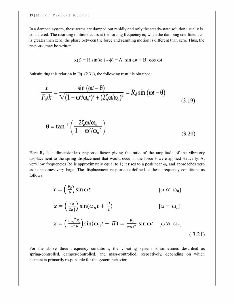
In a damped system, these terms are damped out rapidly and only the steady-state solution usually is
considered. The resulting motion occurs at the forcing frequency ω; when the damping coefficient c
is greater than zero, the phase between the force and resulting motion is different than zero. Thus, the
response may be written
x(t) = R sin(ω t - ϕ) = A1 sin ꙍt + B1 cos ꙍt
Substituting this relation in Eq. (2.31), the following result is obtained:
(3.19)
(3.20)
Here Rd is a dimensionless response factor giving the ratio of the amplitude of the vibratory
displacement to the spring displacement that would occur if the force F were applied statically. At
very low frequencies Rd is approximately equal to 1; it rises to a peak near ωn and approaches zero
as ω becomes very large. The displacement response is defined at these frequency conditions as
follows:
� = � ��
�� sin ꙍ� [ꙍ ≪ ꙍ�]
� = � ��
���� sin(ꙍ�� +
�
�) [ꙍ = ꙍ�]
� = � ꙍ�
���
ꙍ��� sin(ꙍ�� + �) =
��
�ꙍ� sin ꙍ� [ꙍ ≫ ꙍ�]
( 3.21)
For the above three frequency conditions, the vibrating system is sometimes described as
spring-controlled, damper-controlled, and mass-controlled, respectively, depending on which
element is primarily responsible for the system behavior.
18 | M i n o r P r o j e c t R e p o r t
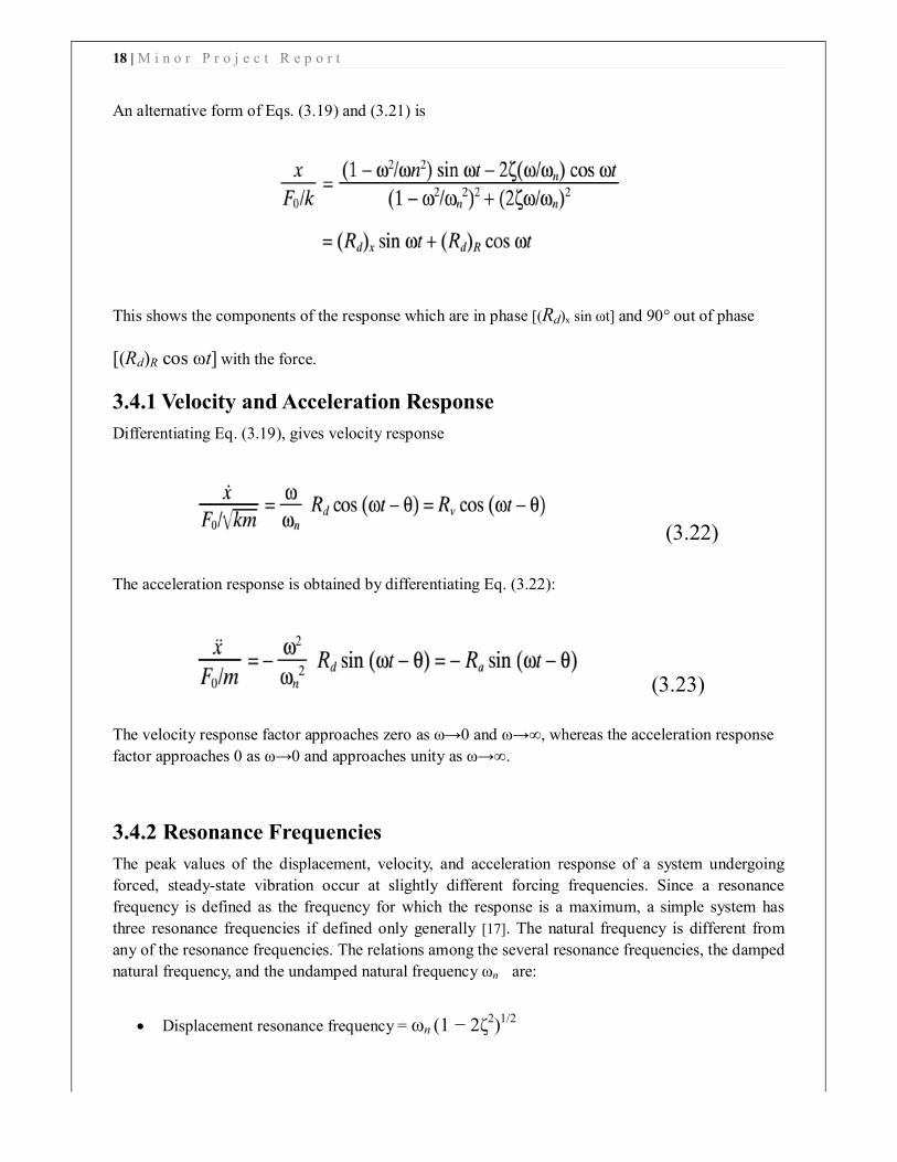
An alternative form of Eqs. (3.19) and (3.21) is
This shows the components of the response which are in phase [(Rd)x sin ωt] and 90° out of phase
[(Rd)R cos ωt] with the force.
3.4.1 Velocity and Acceleration Response
Differentiating Eq. (3.19), gives velocity response
(3.22)
The acceleration response is obtained by differentiating Eq. (3.22):
(3.23)
The velocity response factor approaches zero as ω→0 and ω→∞, whereas the acceleration response
factor approaches 0 as ω→0 and approaches unity as ω→∞.
3.4.2 Resonance Frequencies The peak values of the displacement, velocity, and acceleration response of a system undergoing
forced, steady-state vibration occur at slightly different forcing frequencies. Since a resonance
frequency is defined as the frequency for which the response is a maximum, a simple system has
three resonance frequencies if defined only generally [17]. The natural frequency is different from
any of the resonance frequencies. The relations among the several resonance frequencies, the damped
natural frequency, and the undamped natural frequency ωn are:
Displacement resonance frequency = ωn (1 − 2ζ2)1/2
19 | M i n o r P r o j e c t R e p o r t
Velocity resonance frequency = ωn
Acceleration resonance frequency = ωn/(1 − 2ζ2)1/2
Damped natural frequency = ωn(1 − ζ2)1/2
For the degree of damping usually embodied in physical systems, the difference among the three
resonance frequencies is negligible.
3.5 Two Degrees of Freedom: Vibration
3.5.1 System of Three Springs and Two Masses
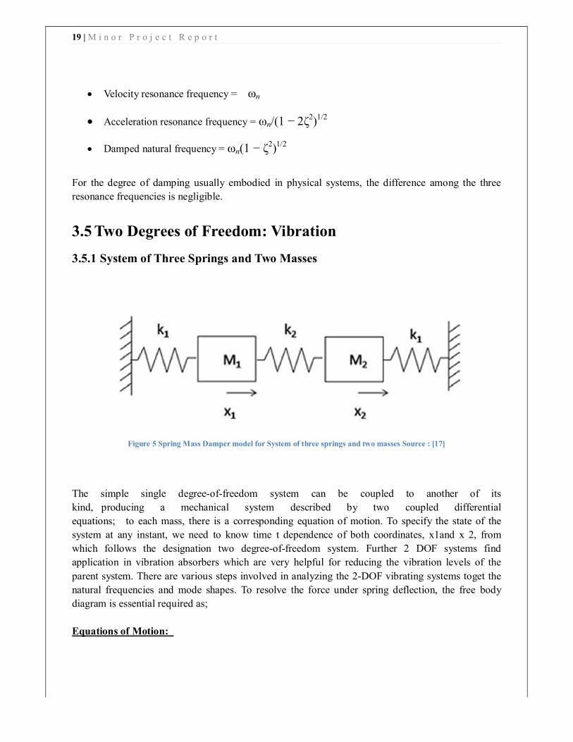
Figure 5 Spring Mass Damper model for System of three springs and two masses Source : [17]
The simple single degree-of-freedom system can be coupled to another of its
kind, producing a mechanical system described by two coupled differential
equations; to each mass, there is a corresponding equation of motion. To specify the state of the
system at any instant, we need to know time t dependence of both coordinates, x1and x 2, from
which follows the designation two degree-of-freedom system. Further 2 DOF systems find
application in vibration absorbers which are very helpful for reducing the vibration levels of the
parent system. There are various steps involved in analyzing the 2-DOF vibrating systems toget the
natural frequencies and mode shapes. To resolve the force under spring deflection, the free body
diagram is essential required as;
Equations of Motion:
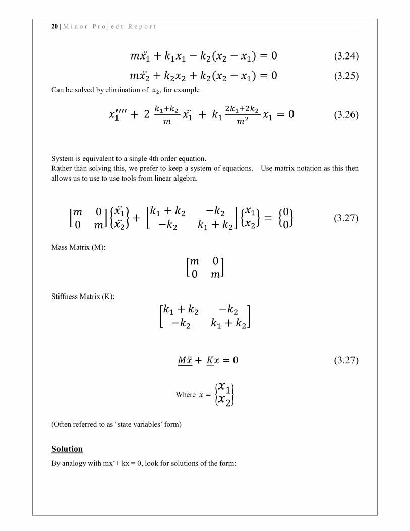
20 | M i n o r P r o j e c t R e p o r t
���̈ + ���� − ��(�� − ��) = 0 (3.24)
���̈ + ���� + ��(�� − ��) = 0 (3.25)
Can be solved by elimination of ��, for example
������ + 2
�����
��� ̈ + ��
�������
�� �� = 0 (3.26)
System is equivalent to a single 4th order equation.
Rather than solving this, we prefer to keep a system of equations. Use matrix notation as this then
allows us to use to use tools from linear algebra.
�� 00 �
� ���̈
��̈� + �
�� + �� −��
−�� �� + ��� �
��
��� = �
00
� (3.27)
Mass Matrix (M):
�� 00 �
�
Stiffness Matrix (K):
��� + �� −��
−�� �� + ���
��̈ + �� = 0 (3.27)
Where � = ��1�2
�
(Often referred to as ‘state variables’ form)
Solution
By analogy with mx¨+ kx = 0, look for solutions of the form:
21 | M i n o r P r o j e c t R e p o r t
���
��� = �
��
��� cos(ꙍ� − �)
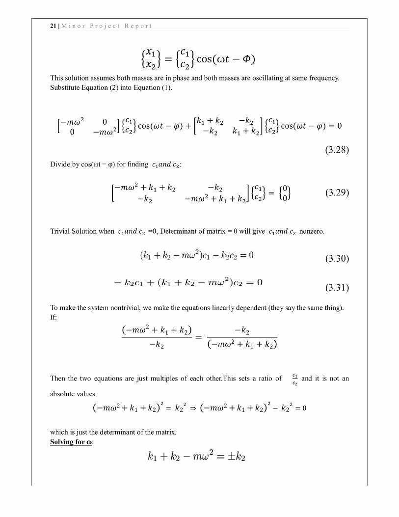
This solution assumes both masses are in phase and both masses are oscillating at same frequency.
Substitute Equation (2) into Equation (1).
�−��� 00 −���� �
��
��� cos(�� − �) + �
�� + �� −��
−�� �� + ��� �
��
��� cos(�� − �) = 0
(3.28)
Divide by cos(ωt − φ) for finding ����� ��:
�−��� + �� + �� −��
−�� −��� + �� + ��� �
��
��� = �
00
� (3.29)
Trivial Solution when ����� �� =0, Determinant of matrix = 0 will give ����� �� nonzero.
(3.30)
(3.31)
To make the system nontrivial, we make the equations linearly dependent (they say the same thing).
If:
(−��2 + �1 + �2)
−�2
= −�2
(−��2 + �1 + �2)
Then the two equations are just multiples of each other.This sets a ratio of ��
�� and it is not an
absolute values.
(−��2 + �1 + �2)�
= �2�
⇒ (−��2 + �1 + �2)�
− �2�
= 0
which is just the determinant of the matrix.
Solving for ω:
22 | M i n o r P r o j e c t R e p o r t
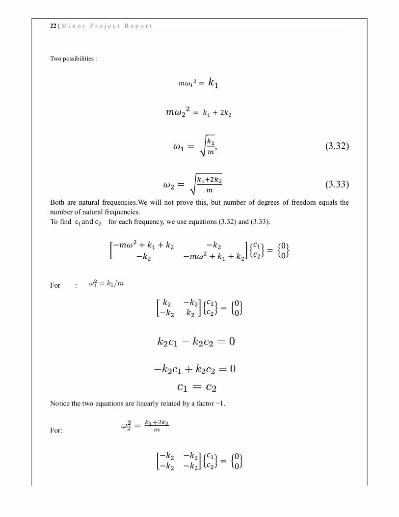
Two possibilities :
���� = �1
����
= �1 + 2�2
�� = ���
�, (3.32)
�� = �������
� (3.33)
Both are natural frequencies.We will not prove this, but number of degrees of freedom equals the
number of natural frequencies.
To find c�and c� for each frequency, we use equations (3.32) and (3.33).
�−��� + �� + �� −��
−�� −��� + �� + ��� �
��
��� = �
00
�
For :
��� −��
−�� ��� �
��
��� = �
00
�
Notice the two equations are linearly related by a factor −1.
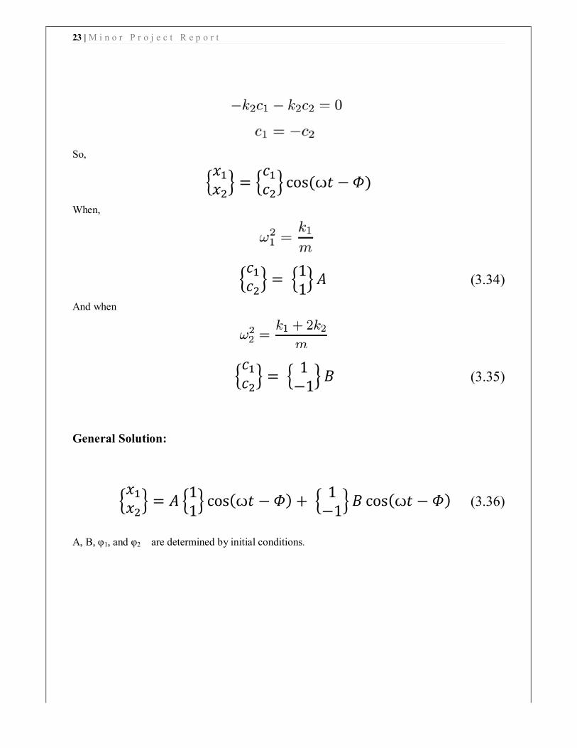
For:
�−�� −��
−�� −��� �
��
��� = �
00
�
23 | M i n o r P r o j e c t R e p o r t
So,
���
��� = �
��
��� cos(ꙍ� − �)
When,
���
��� = �
11
� � (3.34)
And when
���
��� = �
1−1
� � (3.35)
General Solution:
���
��� = � �
11
� cos(ꙍ� − �) + �1
−1� � cos(ꙍ� − �) (3.36)
A, B, φ1, and φ2 are determined by initial conditions.

24 | M i n o r P r o j e c t R e p o r t
3.6 Multiple Degrees of Freedom: Vibration The simple mass–spring damper model is the foundation of vibration analysis. The mass–spring–
damper model described above is called a single degree of freedom (SDOF) model since the mass is
assumed to only move up and down. In the case of more complex systems the system must be
discretized into more masses which are allowed to move in more than one direction – adding degrees
of freedom. The major concepts of multiple degrees of freedom (MDOF) can be understood by looking
at just a 2 degree of freedom model.
Figure 6 Spring Mass Damper model for system of three springs and two masses with dampers Source : [16]
The equations of motion of the 2DOF system are found to be:
This can be rewritten in matrix format:
A more compact form of this matrix equation can be written as:
25 | M i n o r P r o j e c t R e p o r t
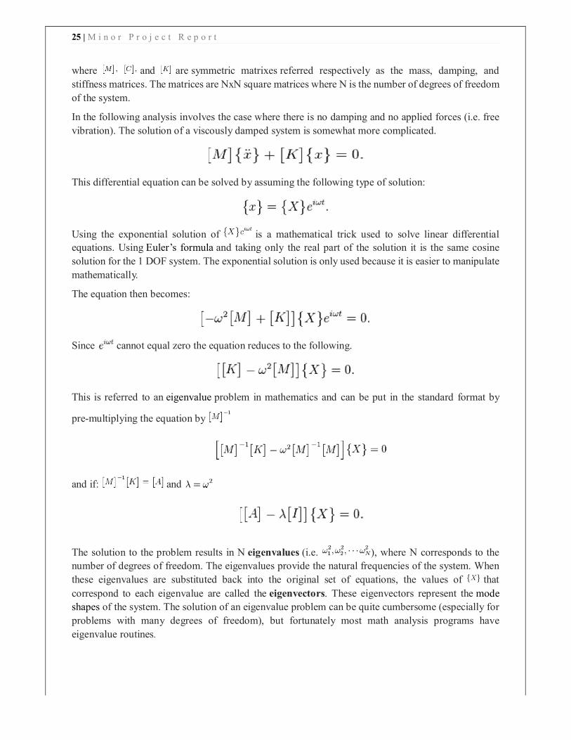
where and are symmetric matrixes referred respectively as the mass, damping, and
stiffness matrices. The matrices are NxN square matrices where N is the number of degrees of freedom
of the system.
In the following analysis involves the case where there is no damping and no applied forces (i.e. free
vibration). The solution of a viscously damped system is somewhat more complicated.
This differential equation can be solved by assuming the following type of solution:
Using the exponential solution of is a mathematical trick used to solve linear differential
equations. Using Euler’s formula and taking only the real part of the solution it is the same cosine
solution for the 1 DOF system. The exponential solution is only used because it is easier to manipulate
mathematically.
The equation then becomes:
Since cannot equal zero the equation reduces to the following.
This is referred to an eigenvalue problem in mathematics and can be put in the standard format by
pre-multiplying the equation by
and if: and
The solution to the problem results in N eigenvalues (i.e. ), where N corresponds to the
number of degrees of freedom. The eigenvalues provide the natural frequencies of the system. When
these eigenvalues are substituted back into the original set of equations, the values of that
correspond to each eigenvalue are called the eigenvectors. These eigenvectors represent the mode
shapes of the system. The solution of an eigenvalue problem can be quite cumbersome (especially for
problems with many degrees of freedom), but fortunately most math analysis programs have
eigenvalue routines.

26 | M i n o r P r o j e c t R e p o r t
27 | M i n o r P r o j e c t R e p o r t
cHApTer: 4
28 | M i n o r P r o j e c t R e p o r t
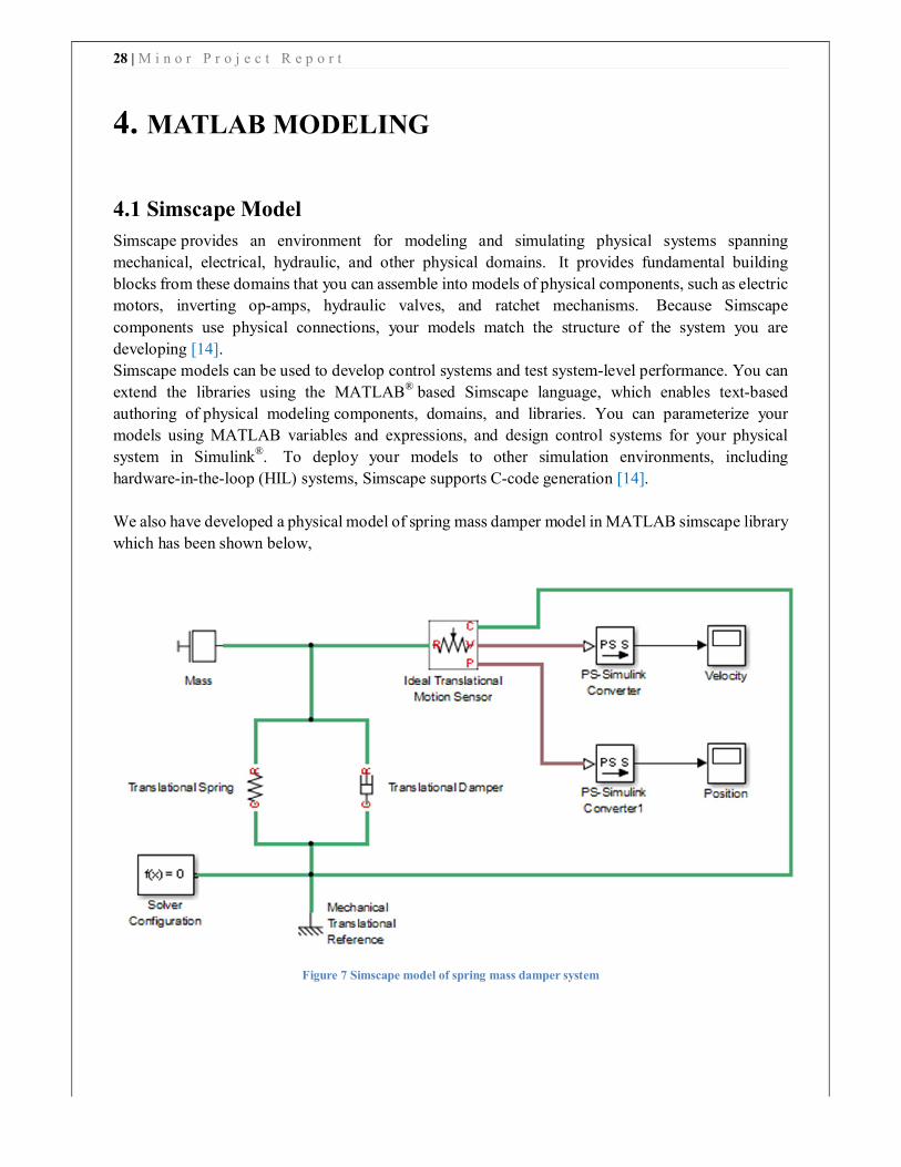
4. MATLAB MODELING
4.1 Simscape Model
Simscape provides an environment for modeling and simulating physical systems spanning
mechanical, electrical, hydraulic, and other physical domains. It provides fundamental building
blocks from these domains that you can assemble into models of physical components, such as electric
motors, inverting op-amps, hydraulic valves, and ratchet mechanisms. Because Simscape
components use physical connections, your models match the structure of the system you are
developing [14].
Simscape models can be used to develop control systems and test system-level performance. You can
extend the libraries using the MATLAB® based Simscape language, which enables text-based
authoring of physical modeling components, domains, and libraries. You can parameterize your
models using MATLAB variables and expressions, and design control systems for your physical
system in Simulink®. To deploy your models to other simulation environments, including
hardware-in-the-loop (HIL) systems, Simscape supports C-code generation [14].
We also have developed a physical model of spring mass damper model in MATLAB simscape library
which has been shown below,
Figure 7 Simscape model of spring mass damper system

29 | M i n o r P r o j e c t R e p o r t
4.2 Simulink Model
Simulink is a block diagram environment for multidomain simulation and Model-Based Design. It
supports simulation, automatic code generation, and continuous test and verification of embedded
systems [15].
Simulink provides a graphical editor, customizable block libraries, and solvers for modeling and
simulating dynamic systems. It is integrated with MATLAB®, enabling you to incorporate MATLAB
algorithms into models and export simulation results to MATLAB for further analysis [15].
We also have developed a Simulink model for differential eqation of vibration which is shown below,
Figure 8 Simulink model of Spring Mass Damper Vibration
30 | M i n o r P r o j e c t R e p o r t
cHApTer: 5

31 | M i n o r P r o j e c t R e p o r t
5. VIBRATIONAL ANALYSER (VIBXPERT II)
The best way of vibration analysis is that through the frequency analysis. The frequency analysis
involves a frequency spectrum which provides us with the detailed information of the signal sources
not able to be obtained from the time signal. It provides information on the vibrations caused due to
rotating parts and tooth meshing. Hence it plays a very valuable role in locating regions of
undesirable vibrations.
Frequency analysis process involves sending a signal through a filter and at the same time sweeping
the filter over the frequency range of filters; it is possible to get a measure of the signal level at
different frequencies which in turn gives us the frequency spectrum.
2 examples of monitoring:
Monitoring of a fan: The most likely fault to occur is unbalance, which will give an increase in the
vibration level at the speed of rotation. This will normally also be the highest level in the spectrum.
To see if unbalance is developing, it is therefore sufficient to measure the overall level at regular
intervals. The overall level will reflect the increase just as well as the spectrum.
Monitoring of a gearbox: Damaged or worn gears will show up as an increase in the vibration level
at the tooth meshing frequencies (shaft RPM number of teeth) and their harmonics. The levels at
these frequencies are normally much lower than the highest level in the frequency spectrum, so it is
necessary to use a full spectrum comparison to reveal a developing fault.
Presenting the data:
The data is presented in the form of linear scales with ranges dictated by the range of data but it does
not allow seeing some important data. Hence logarithmic scales are used.
VIBXPERT is a device that helps in vibrations analysis. It provides us with many key functions as:
1. Route based data collection.
2. Vibration diagnosis
3. Field balancing.
4. Multimeter
5. Data logging
6. Visual inspection
7. Print reports on USB stick.
8. Time waveform.
9. Amplitude spectrum.
10. Static shaft position (for balancing)
11. Long term recording
12. Printing of measurement reports.
We are using this analyser to analyse forced and cutting vibrations in different machining processes.
From obtained result we finally anlyse how to reduce these chatter vibrations.
32 | M i n o r P r o j e c t R e p o r t
cHApTer: 6
33 | M i n o r P r o j e c t R e p o r t
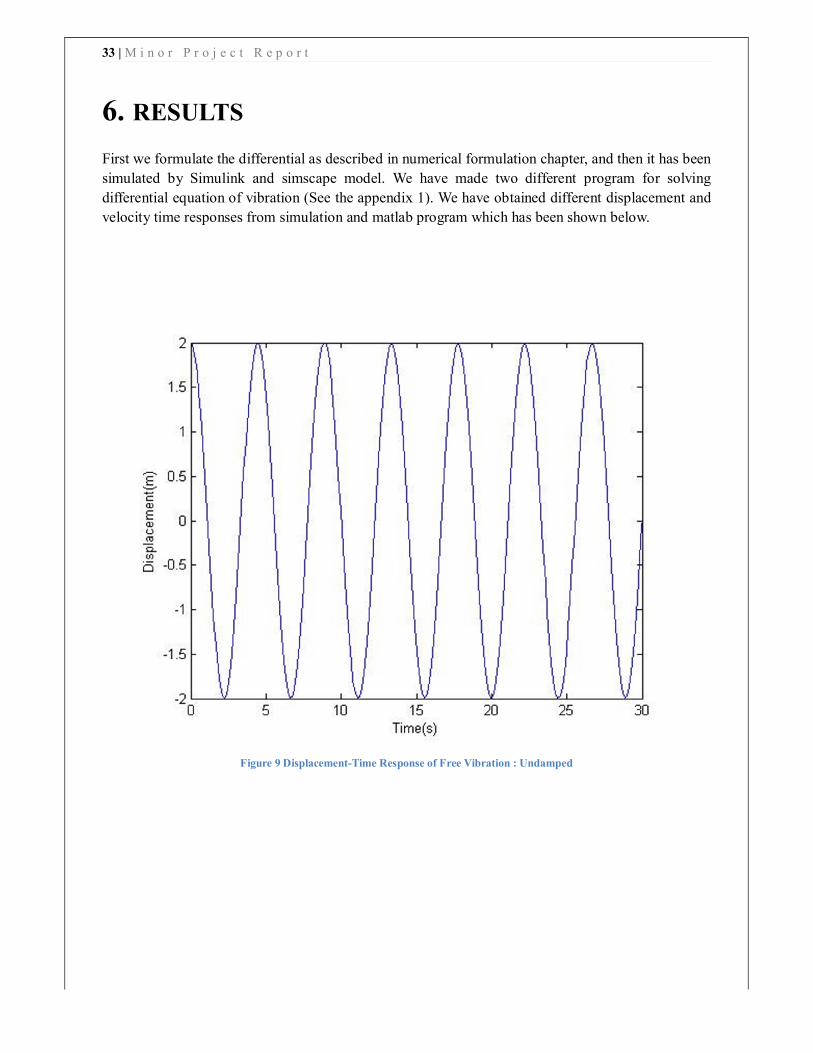
6. RESULTS
First we formulate the differential as described in numerical formulation chapter, and then it has been
simulated by Simulink and simscape model. We have made two different program for solving
differential equation of vibration (See the appendix 1). We have obtained different displacement and
velocity time responses from simulation and matlab program which has been shown below.
Figure 9 Displacement-Time Response of Free Vibration : Undamped

34 | M i n o r P r o j e c t R e p o r t
Figure 10 Velocity-Time Responce of Free Vibration: Undamped
Figure 11 Velocity-Time Responce of damped Free Vibration: Critically Damped
35 | M i n o r P r o j e c t R e p o r t
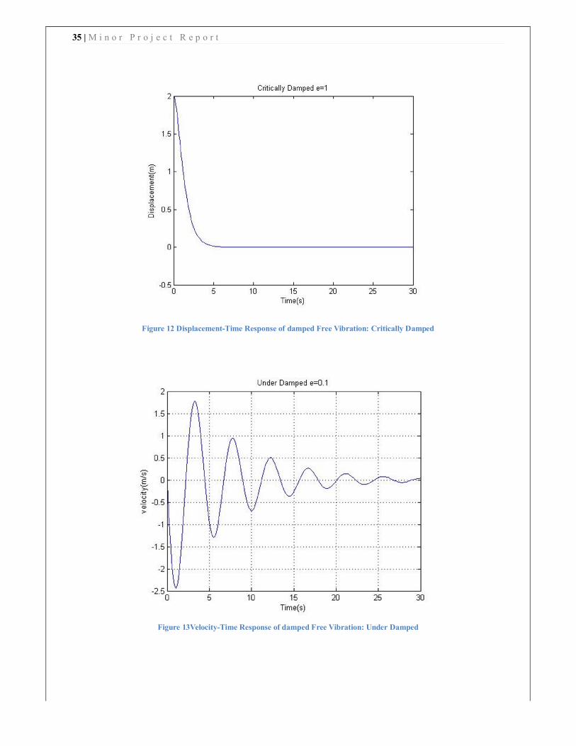
Figure 12 Displacement-Time Response of damped Free Vibration: Critically Damped
Figure 13Velocity-Time Response of damped Free Vibration: Under Damped

36 | M i n o r P r o j e c t R e p o r t
Figure 14 Displacement-Time Responce of damped Free Vibration: Under Damped
Figure 15 Displacement-Time Response of damped Free Vibration: Over Damped

37 | M i n o r P r o j e c t R e p o r t
Figure 16 Velocity-Time Response of damped Free Vibration: Over Damped
Figure 17 Displacement-Time Response of Forced Vibration: Undamped

38 | M i n o r P r o j e c t R e p o r t
Figure 18 Velocity-Time Response Of Forced Vibration: Undamped
Figure 19 Displacement-Time Response of damped Forced Vibration: Critically Damped
39 | M i n o r P r o j e c t R e p o r t
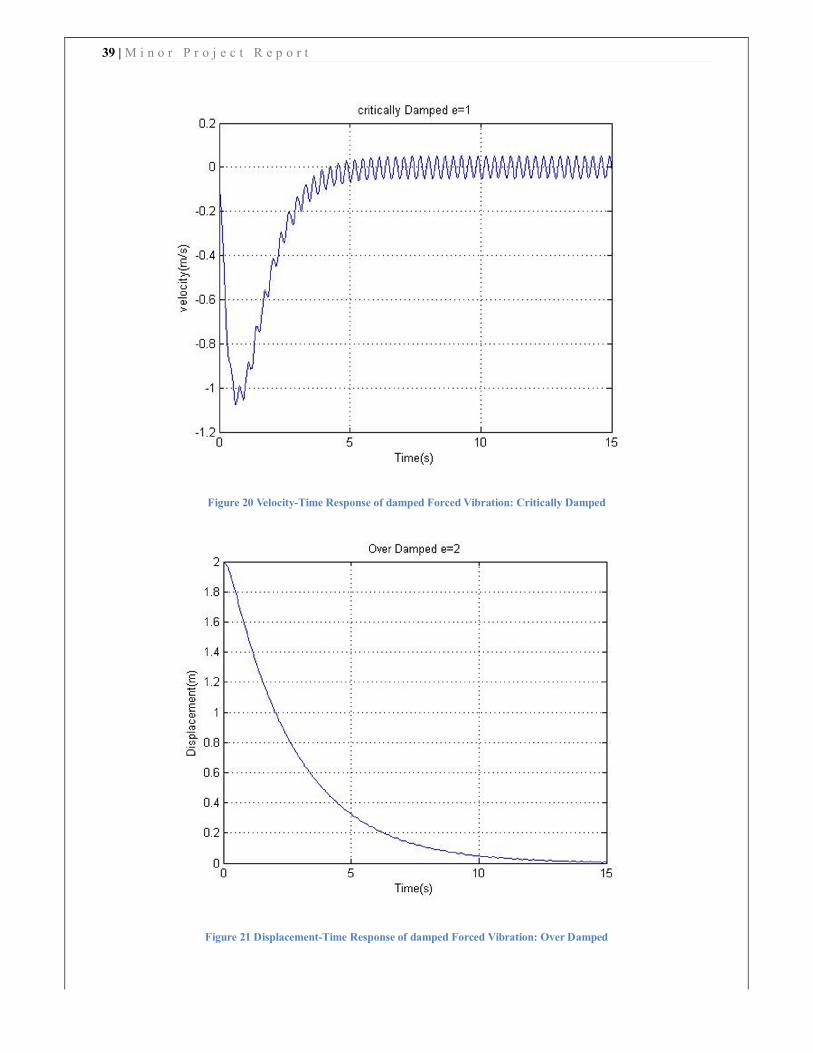
Figure 20 Velocity-Time Response of damped Forced Vibration: Critically Damped
Figure 21 Displacement-Time Response of damped Forced Vibration: Over Damped

40 | M i n o r P r o j e c t R e p o r t
Figure 22 Velocity -Time Response of damped Forced Vibration: Over Damped
Figure 23 Displacement-Time Response of damped Forced Vibration: Under Damped

41 | M i n o r P r o j e c t R e p o r t
Figure 24 Velocity -Time Response of damped Forced Vibration: Under Damped

42 | M i n o r P r o j e c t R e p o r t
cHApTer: 7
43 | M i n o r P r o j e c t R e p o r t
7. CONCLUSION
In this study, we examined different very basic type of vibration for spring mass damper system with
and without damping. The simulation model and differential equation were established and solved
using MATLAB for modal natural frequency and time response. Displacement and velocity time
response were obtained for different type of vibration. We can easily see the how different factor
affect the natural frequency.
In this study, we have studied the vibxpert vibrational analyser which can easily analyse vibration
produced in various machining processes and represent it in easy to understand form. We are using
this vibration analyser in analyzing different type of vibration produced in machining processes.

44 | M i n o r P r o j e c t R e p o r t
references

45 | M i n o r P r o j e c t R e p o r t
Bibliography
1. Tobias, S.A. Machine Tool Vibration. Spain : UMRO, 1961.
2. Chatter in machining process: A review. Guillem Quintana, Joquim Ciurana. 2011, International Journal of
Machine tools and Manufacture, pp. 363-376.
3. S.A. Tobais, W. Fishwick. Theory of regenerative machine tool chatter. s.l. : The Engineer, 1958.
4. A review of chatter vibration research in turning. M. Siddhpura, R. Paurobally. 1, s.l. : ELSEVIER, 2012,
International Journal of machine tools and manufacture, Vol. 61, pp. 27-47.
5. On the art of cutting metals. F.Taylor. 1907, Transactions of ASME , Vol. 28.
6. The stability of machine tools against self-excited vibrations in machining. J. Tlusty, M. Polacek. 1963,
International Research in Production Engineering, pp. 465–474.
7. Theory of self-excited machine-tool chatter-contribution to machine tool chatter research—1. Merrit, H.E. 1965,
ASME Journal of Engineering for Industry, pp. 447-454.
8. Robust Analysis of Stability in Internal Turning. Giovanni Totis, Marco Sortino. Udine, Italy : ELSEVIER,
2014. 24th DAAAM International Symposium on Intelligent Manufacturing and Automation. Vol. 69, pp.
1306-1315.
9. Viscous damping identification in linear vibration. S. Adhikari, J. Woodhouse. 2007, Journal of Sound and
Vibration , Vol. 303, pp. 475-500.
10. Jiao Chunwang, Liu Jie, Guo Dameng and Wang Qianqian. A New Method for Solving Nonlinear Forced
Vibration System Response. 2010.
11. Wahab, M. A. Dynamics and Vibration: An Introduction. s.l. : John Wiley & Sons Ltd., 2008.
12. Rattan, S.S. Theory of Machines. 3. New Delhi : McGraw Hill Education (India) Private Ltd., 2009.
13. Study of the correlation between surface generation and cutting vibrations in peripheral milling. Hao Jiang,
Xinhua Long, Guang Meng. Shanghai, China : s.n., 2008, journal of materials processing technology, Vol. 208, pp.
229-238.
14. Simulink: Simulation and model based design, MathsWorks [viewed by 16 oct 2014] Available from
https://in.mathworks.com/products/simulink/
15. Physical System Simulation, Mathswork [viewed by 16 oct 2014]. Available from
http://in.mathworks.com/products/simscape/
16. Vibration, Wikipedia : The free encyclopedia [viewed by 8 oct 2014] Available from
http://en.wikipedia.org/wiki/Vibration
17. Blake R. E. Basic Vibration theory, s.1: John Wiley & Sons Ltd., 2009.

46 | M i n o r P r o j e c t R e p o r t
Appendix 1

47 | M i n o r P r o j e c t R e p o r t
MATLAB Programme for analyzing free vibration characteristics time response:
For solution of equation (1.2) , at first we have to make a following function in MATLAB;
function rk = f(t,y)
rk = zeros(2,1);
k=10; %N/m
m=5; %Kg
rk(1)= y(2);
rk(2)= (-k/m)*y(1);
Here rk is a vector solution of our differential equation which is stored in function named f, k is the
stiffness of spring and m is mass. y(1) is displacement of mass at anytime t and y(2) is velocity of
mass. We can say,
y(1) = x(t);
y(2) = ��(�)
�� = v(t);
After making above function main script is given below;
clear all;
timerange= [0 30]; %sec
initialvalues = [2 0];
[t,y]=ode45(@f,timerange,initialvalues);
plot(t,y(:,1))
ylabel('Displacement(m)')
xlabel('Time(s)')
figure
plot(t,y(:,2))
ylabel('velocity(m/s)')
xlabel('Time(s)')
Here timerange is range of time for which we are going to plot the time response of spring mass
system which is from 0 to 30 seconds. Initialvalues function is defined for setting initial values of y(1)
and y(2) which are 2 and 0 m/s. ODE45 is differential solver function of matlab.
MATLAB Programme for analyzing damped free vibration characteristics time
48 | M i n o r P r o j e c t R e p o r t
response:
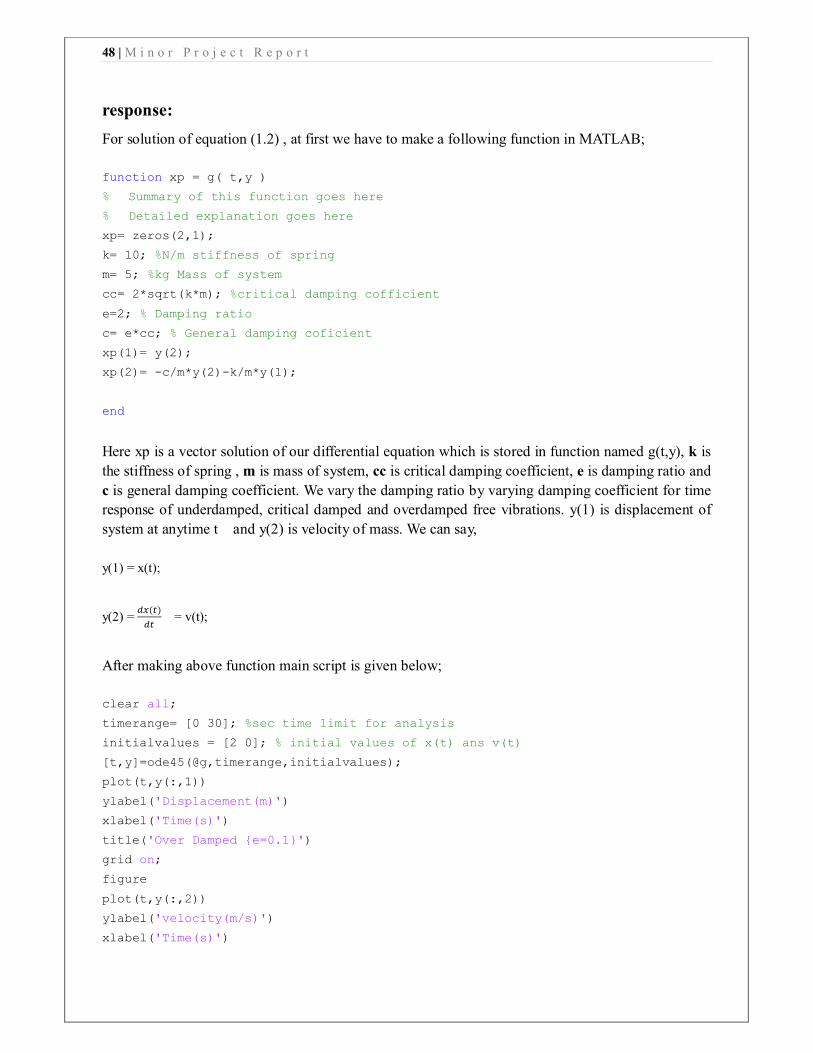
For solution of equation (1.2) , at first we have to make a following function in MATLAB;
function xp = g( t,y )
% Summary of this function goes here
% Detailed explanation goes here
xp= zeros(2,1);
k= 10; %N/m stiffness of spring
m= 5; %kg Mass of system
cc= 2*sqrt(k*m); %critical damping cofficient
e=2; % Damping ratio
c= e*cc; % General damping coficient
xp(1)= y(2);
xp(2)= -c/m*y(2)-k/m*y(1);
end
Here xp is a vector solution of our differential equation which is stored in function named g(t,y), k is
the stiffness of spring , m is mass of system, cc is critical damping coefficient, e is damping ratio and
c is general damping coefficient. We vary the damping ratio by varying damping coefficient for time
response of underdamped, critical damped and overdamped free vibrations. y(1) is displacement of
system at anytime t and y(2) is velocity of mass. We can say,
y(1) = x(t);
y(2) = ��(�)
�� = v(t);
After making above function main script is given below;
clear all;
timerange= [0 30]; %sec time limit for analysis
initialvalues = [2 0]; % initial values of x(t) ans v(t)
[t,y]=ode45(@g,timerange,initialvalues);
plot(t,y(:,1))
ylabel('Displacement(m)')
xlabel('Time(s)')
title('Over Damped {e=0.1}')
grid on;
figure
plot(t,y(:,2))
ylabel('velocity(m/s)')
xlabel('Time(s)')

49 | M i n o r P r o j e c t R e p o r t
title('Over Damped {e=0.1}')
grid on;
Here timerange is range of time for which we are going to plot the time response of spring mass
system which is from 0 to 30 seconds. Initialvalues function is defined for setting initial values of y(1)
and y(2) which are 2 and 0 m/s. ODE45 is differential solver function of matlab.


