Laboratory Skills

Experiment – A Trying Out ActionStep 1 Understand the principles involved in the procedure of the experiment

Step 2 Your skill in arranging and handling different measuring instruments

Step 3 Determination of errors in various measurements and planning/suggesting how

these contributions may be made of the same order so as to make the error in the

final result small

Step 4 A comprehensive view of the whole experiment with sufficient number of

observations, correct calculations, proper graphs and result

Problem Solving - An Effective Approach AidHint 1 Read the problem carefully

Hint 2 Understand what is given and what is required Write down the given data, with units, using the symbols What is the unknown and what is its symbol What is the connection between the unknown and the data

Hint 3 Watch the units You may need to make conversions

Hint 4 Think about your answer Whether it makes sense Is the sign correct Are the units appropriate

Hint 5 Reading the graph Note the units in which the variables are expressed Note the variables whether positive or negative A graph describes something that is happening and you should be able to

say what it is

Laboratory Skills

6.1(a) Band Gap Determination using Post Office Box

Aim

To find the band gap of the material of the given thermistor using post office box.

Apparatus Required

Thermistor, thermometer, post office box, power supply, galvanometer, insulating coil and glass beakers.

Principle and formulae

(1) Wheatstone’s Principle for balancing a network

PQ

=RS

Of the four resistances, if three resistances are known and one is unknown, the unknown resistance can be calculated.

(2) The band gap for semiconductors is given by,

Eg = 2k( 2. 303 loge RT

1T

)

where k = Boltzmann constant = 1.38 10 – 23 J /K

RT = Resistance at T K

Procedure

1. The connections are given as in the Fig. 6.1(a).1. Ten ohm resistances are taken in P and Q.

2. Then the resistance in R is adjusted by pressing the tap key, until the deflection in the galvanometer crosses zero reading of the galvanometer, say from left to right.

3. After finding an approximate resistance for this, two resistances in R, which differ by 1 ohm, are to be found out such that the deflections in the galvanometer for these resistances will be on either side of zero reading of galvanometer.

4. We know RT =

QP

× R = 1010

× R1 or (R1+1).This means that the resistance of the

thermistor lies between R1 and (R1+1). Then keeping the resistance in Q the same, the resistance in P is changed to 100 ohm.

5. Again two resistances, which differ by one ohm are found out such that the deflections in the galvanometer are on the either side of zero. Therefore the actual

resistance of thermistor will be between

R2

10 and

R2 + 110

.

6.2

Materials Science

Table 6.1(a).1 To find the resistance of the thermistor at different temperatures

Temp. of thermistorT = t+273

1T

Resistance in P

Resistance in Q

Resistance in R

Resistance of the thermistor

RT =

PQ R

2.303 log10 RT

K K-1 ohm ohm Ohm ohm ohm

Fig 6.1(a).1 Post Office Box - Circuit diagram Fig 6.1(a).2 Model Graph

Observation

From graph, slope = (dy / dx) = ……

Calculation

Band gap, Eg = 2k(dy / dx) =…..

6. Then the resistance in P is made 1000 ohms keeping same 10 ohms in Q. Again, two resistances R and (R+1) are found out such that the deflection in galvanometer changes its direction. Then the correct resistance.

=

RT =101000

( R )

(or)

6.3

Laboratory Skills

= R+1 = 0.01R (or) 0.01(R+1)

7. Thus, the resistance of the thermistor is found out accurately to two decimals, at room temperature. The lower value may be assumed to be RT (0.01R).

8. Then the thermistor is heated, by keeping it immersed in insulating oil. For every 10 K rise in temperature, the resistance of the thermistor is found out, (i.e) RT

’s are found out. The reading is entered in the tabular column.

Graph

A graph is drawn between

1T

in X axis and 2.303 log RT in Y axis where T is the temperature in K and RT is the resistance of the thermistor at TK. The graph will be as shown in the Fig.6.1(a).2.

Band gap (Eg)=2k slope of the graph = 2k (

dydx

)

where K = Boltzman’s constant.

Result

The band gap of the material of the thermistor = ………eV.

6.4

Materials Science

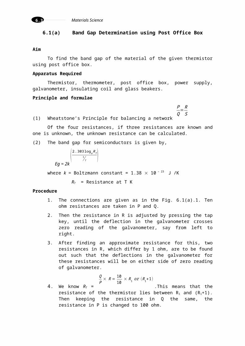
6.1(b) Resistivity Determination for a Semiconductor Wafer using Four Probe Method

AimTo determine the energy band gap of a semiconductor (Germanium) using four probe

method.Apparatus Required

Probes arrangement (it should have four probes, coated with zinc at the tips). The probes should be equally spaced and must be in good electrical contact with the sample), Sample (Germanium or silicon crystal chip with non-conducting base), Oven (for the variation of temperature of the crystal from room temperature to about 200°C), A constant current generator (open circuit voltage about 20V, current range 0 to 10mA), Milli-voltmeter (range from 100mV to 3V), Power supply for oven Thermometer.Formula The energy band gap, Eg., of semi-conductor is given by

Eg = 2k B

2 .3026 × log10 ρ1

T

in eV

where kB is Boltzmann constant equal to 8.6 × 10 – 5 eV / kelvin , and is the resistivity of the semi-conductor crystal given by

ρ =ρ0

f (W /S )where ρ0 = V

I×2 πs

; ρ = V

I(0 .213)

Here, s is distance between probes and W is the thickness of semi-conducting crystal. V and I are the voltage and current across and through the crystal chip.Procedure

1. Connect one pair of probes to direct current source through milliammeter and other pair to millivoltmeter.

2. Switch on the constant current source and adjust current I, to a described value, say 2 mA.

3. Connect the oven power supply and start heating.4. Measure the inner probe voltage V, for various temperatures.

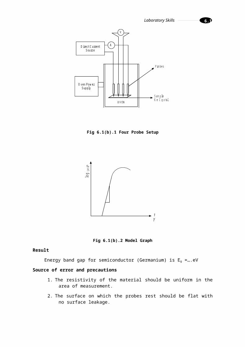
Graph

Plot a graph in (103

T ) and log10 as shown in Fig.6.1(b).2. Find the slope of the curve

ABBC

=log10 ρ

103

T . So the energy band gap of semiconductor (Germanium) is given by

Eg = 2 k×2 .3026 × log10 ρ

1/T

= 2×8 . 6×10−5×2. 3026× AB

CD×1000 eV=0. 396× AB

CDeV

6.5

Laboratory Skills

Table 6.1(b).1 To determine the resistivity of the semi-conductor for various temperatures:

Current (I) = …………mA

S.No.Temperature Voltage (V) Resistivity

(ohm. cm)10 – 3 / T

Log10in°C in K (Volts) (K)

Observations:

Distance between probes(s) = ……………………..mm

Thickness of the crystal chip (W) = ……………………mm

current (I) = ………………..mA

6.6

Materials Science

Fig 6.1(b).1 Four Probe Setup

Fig 6.1(b).2 Model Graph

Result

Energy band gap for semiconductor (Germanium) is Eg =….eV

Source of error and precautions

1. The resistivity of the material should be uniform in the area of measurement.

2. The surface on which the probes rest should be flat with no surface leakage.

3. The diameter of the contact between the metallic probes and the semiconductor crystal chip should be small compared to the distance between the probes.

6.7

Laboratory Skills

6.2 Determination of Hall Coefficient and carrier type for a Semi-conducting Material

Aim

To determine the hall coefficient of the given n type or p-type semiconductor

Apparatus Required

Hall probe (n type or p type), Hall effect setup, Electromagnet, constant current power supply, gauss meter etc.,

Formulae

i) Hall coefficient (RH) =

V H . tIH

× 10 8 cm3 C – 1

where VH = Hall voltage (volt)

t = Thickness of the sample (cm)

I = Current (ampere)

H = Magnetic filed (Gauss)

ii) Carrier density ( n ) =

1RH q

cm – 3

where RH = Hall coefficient (cm3 C – 1 )

q = Charge of the electron or hole (C)

iii) Carrier mobility ( ) = RH cm2V – 1 s – 1

where RH = Hall coefficient (cm3C – 1 )

= Conductivity (C V – 1 s – 1 cm – 1 )

Principle

Hall effect: When a current carrying conductor is placed in a transverse magnetic field, a potential difference is developed across the conductor in a direction perpendicular to both the current and the magnetic field.

6.8

Materials Science

Table 6.2.1 Measurement of Hall coefficient

Current in the Hall effect setup = ----------mA

Current in the constant current

power supply (A)

Magnetic field (H)(Gauss)

Hall Voltage (VH)(volts)

Hall coefficient (RH)cm3 C – 1

Observations and Calculations

(1) Thickness of the sample = t = cm

(2) Resistivity of the sample = = V C – 1 s cm

(3) Conductivity of the sample = = CV – 1 s – 1 cm – 1

(4) The hall coefficient of the sample = RH =

V H . tIH

× 10 8

= -------------

(5) The carrier density of the sample = n =

1RH q

= -------------

(6) The carrier mobility of the sample= RH

= ---------------

6.9

Laboratory Skills

Fig 6.2.1 Hall Effect Setup

Procedure

1. Connect the widthwise contacts of the hall probe to the terminals marked as ‘voltage’ (i.e. potential difference should be measured along the width) and lengthwise contacts to the terminals marked (i.e. current should be measured along the length) as shown in fig.

2. Switch on the Hall Effect setup and adjust the current say 0.2 mA.

3. Switch over the display in the Hall Effect setup to the voltage side.

4. Now place the probe in the magnetic field as shown in fig and switch on the electromagnetic power supply and adjust the current to any desired value. Rotate the Hall probe until it become perpendicular to magnetic field. Hall voltage will be maximum in this adjustment.

5. Measure the hall voltage and tabulate the readings.

6. Measure the Hall voltage for different magnetic fields and tabulate the readings.

7. Measure the magnetic field using Gauss meter

8. From the data, calculate the Hall coefficient, carrier mobility and current density.

Result

1. The Hall coefficient of the given semi conducting material =

2. The carrier density =

3. The carrier mobility =

6.10

Materials Science

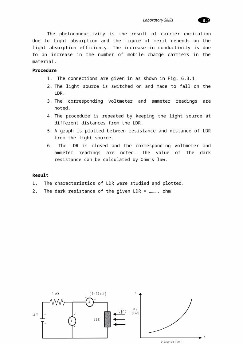
6.3. To study V-I Characteristics of a Light Dependent Resistor (LDR)

AimTo measure the photoconductive nature and the dark resistance of the given light

dependent resistor (LDR) and to plot the characteristics of the LDR.

Apparatus Required LDR, Resistor (1 k), ammeter (0 – 10 mA), voltmeter (0 – 10 V), light source, regulated

power supply.

Formula

By ohm’s law, V=IR (or) R=V

I ohmwhere R is the resistance of the LDR (i.e) the resistance when the LDR is closed. V and I

represents the corresponding voltage and current respectively.

PrincipleThe photoconductive device is based on the decrease in the resistance of certain

semiconductor materials when they are exposed to both infrared and visible radiation.

The photoconductivity is the result of carrier excitation due to light absorption and the figure of merit depends on the light absorption efficiency. The increase in conductivity is due to an increase in the number of mobile charge carriers in the material.

Procedure1. The connections are given in as shown in Fig. 6.3.1.2. The light source is switched on and made to fall on the LDR.3. The corresponding voltmeter and ammeter readings are noted.4. The procedure is repeated by keeping the light source at different distances from the

LDR.5. A graph is plotted between resistance and distance of LDR from the light source.6. The LDR is closed and the corresponding voltmeter and ammeter readings are noted.

The value of the dark resistance can be calculated by Ohm’s law.

Result1. The characteristics of LDR were studied and plotted.2. The dark resistance of the given LDR = …….. ohm

6.11

Laboratory Skills

Fig. 6.3.1 Circuit diagram Fig.6.3.2 Model graph

Observation

Voltmeter reading when the LDR is closed = …… V

Ammeter reading when the LDR is closed = ……. A

Dark resistance =

R=VI

= ……. ohm

Table 6.3.1 To determine the resistances of LDR at different distances

S.No

Distance

(cm)

Voltmeter reading

(V) volt

Ammeter reading

(I) mA

RR

k

6.12

Materials Science

6.4 Determination of Energy Loss in a Magnetic Material – B-H Curve

Aim

(i) To trace the B-H loop (hysteresis) of a ferrite specimen (transformer core) and

(ii) To determine the energy loss of the given specimen.

Apparatus Required

Magnetizing coil, CRO, given sample of ferrite etc.,

Principle

The primary winding on the specimen, when fed to low a.c. voltage (50 Hz), produces a magnetic field H of the specimen. The a.c. magnetic field induces a voltage in the secondary coil. The voltage across the resistance R1, connected in series with the primary is proportional to the magnetic field and is given to the horizontal input of CRO. The induced voltage in the secondary coil, which is proportional to dB/dt (flux density), is applied to the passive integrating circuit. The output of the integrator is now fed to the vertical input of the CRO. Because of application of a voltage proportional to H to the horizontal axis and a voltage proportional to B to the vertical axis, the loop is formed as shown in figure.

Formula

Energy loss =

N1

N 2×

R2

R1×

C2

AL× SV SH ׿ ¿

Area of loop Unit: Joules / cycle / unit vol.

where N1 = number of turns in the Primary

N2 = number of turns in the Secondary

R1 = Resistance between D to A or D to B or D to C

R2 = Resistance between upper S and V (to be measured by the student on B-H unit)

C2 = Capacitance

A = Area of cross section = w t (m)

L = Length of the specimen =2 (length + breadth) (m)

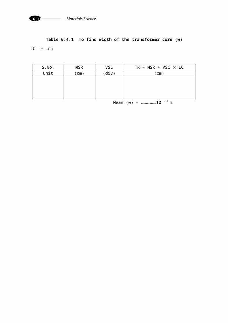
Table 6.4.1 To find width of the transformer core (w)

LC = …cm

S.No. MSR VSC TR = MSR + VSC LCUnit (cm) (div) (cm)

6.13

Laboratory Skills

Mean (w) = ………………10 – 2 m

6.14

Materials Science

Table 6.4.2 To find thickness of the transformer core (t)

LC =… cm

S.No. MSR VSC TR = MSR + VSC LCUnit (cm) (div) (cm)

Mean (t) = ………………10 – 2 m

Observations

N1 = Number of turns in the Primary = 200 turns

N2 = Number of turns in the Secondary = 400 turns

R2 = Resistance between upper S and V = 4.7 kilo-ohm

C2 = Capacitance = 4.7µF

A = Area of cross section (w t) =… m2

L = Length of the specimen = 2(length + breadth) = … m

w = Width of the transformer core =… m

t = Thickness of the specimen =… m

R1 = Resistance between D to A or D to B or D to C =

Sv = Vertical sensitivity of CRO =

SH = Horizontal sensitivity of CRO =

Fig 6.4.1 Experimental Arrangement

6.15

Laboratory Skills

Fig 6.4.2 Hysteresis Loop Fig 6.4.3 Top view of BH curve Unit

Table 6.4.3 To find breadth of the transformer core (w)

LC = …cm

S.No. MSR VSC TR = MSR + VSC X LCUnit (cm) (div) (cm)

Mean (b) = ………………10 – 2 m

Table 6.4.4 To find length of the transformer core (l)

LC =… cm

S.No. MSR VSC TR = MSR + VSC LCUnit (cm) (div) (cm)

Mean (l) = ………………10 – 2 m

Procedure

1. Choose appropriate resistance values by connecting terminal D to either A,B or C.

2. Connect the primary terminals of the specimen to P,P and secondary to S, S terminals.

3. Calibrate the CRO.

4. Adjust the CRO to work on external mode. The time is switched off. Adjust horizontal and vertical position controls such that the spot is at the centre of the CRO screen.

5. Connect terminal marked GND to the ground of the CRO.

6. Connect terminal H to the horizontal input of the CRO.

6.16

Materials Science

7. Connect terminal V to the vertical input of the CRO.

8. Switch ON the power supply of the unit. The hysteresis loop is formed.

9. Adjust the horizontal and vertical gains such that the loop occupies maximum area on the screen of the CRO. Once this adjustment is made, do not disturb the gain controls.

10. Trace the loop on a translucent graph paper. Estimate the area of loop.

11. Remove the connections from CRO without disturbing the horizontal and vertical gain controls.

12. Determine the vertical sensitivity of the CRO by applying a known AC voltage, say 6V (peak to peak). If the spot deflects x cm, for 6V the sensitivity = (6/x 10 – 2 volts / metre. Let it be Sv.

13. Determine the horizontal sensitivity of the CRO by applying a known AC voltage, say 6V (peak to peak). Let the horizontal sensitivity be SH volts / metre.

14. The energy loss is computed from the given formula.

Result

Energy loss of the transformer core is given as _____________ Joules/cycle/unit vol.

6.17

Laboratory Skills

6.5. Determination of Paramagnetic Susceptibility – Quincke’s Method

Aim

To measure the susceptibility of paramagnetic solution by Quincke’s tube method.

Apparatus Required

Quincke’s tube, Travelling microscope, sample (FeCl3 solution), electromagnet, Power supply, Gauss meter.

Principle

Based on molecular currents to explain Para and diamagnetic properties magnetic moment to the molecule and such substances are attracted in a magnetic filed are called paramagnetics. The repulsion of diamagnetics is assigned to the induced molecular current and its respective reverse magnetic moment.

The force acting on a substance, of either repulsion or attraction, can be measured with the help of an accurate balance in case of solids or with the measurement of rise in level in narrow capillary in case of liquids.

The force depends on the susceptibility , of the material, i.e., on ratio of intensity of magnetization to magnetizing field I/H. If the force on the substance and field are measured the value of susceptibility can be calculated.

Formula

The susceptibility of the given sample is found by the formula

=

2( ρ−σ )ghH2

kg m– 1 s– 2 gauss– 2

Where is the density of the liquid or solution (kg/m3)

is the density of air (kg/ m3)

g is the acceleration due to gravity (ms-2)

h is the height through which the column rises (m)

H is the magnetic field at the centre of pole pieces (Gauss)

6.18

Materials Science

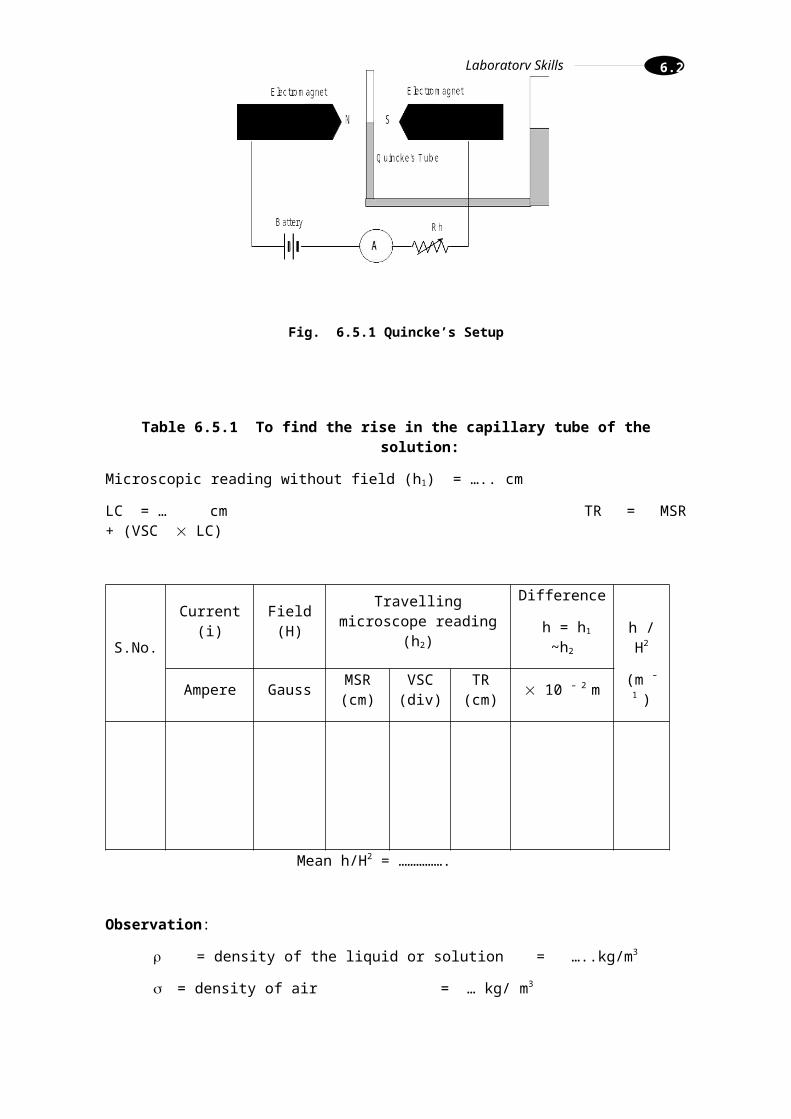
Fig. 6.5.1 Quincke’s Setup

Table 6.5.1 To find the rise in the capillary tube of the solution:

Microscopic reading without field (h1) = ….. cm

LC = … cm TR = MSR + (VSC LC)

S.No.Current (i) Field (H) Travelling microscope

reading (h2)Difference

h = h1 ~h2 h / H2

(m – 1 )Ampere Gauss MSR (cm)

VSC (div)

TR (cm) 10 – 2 m

Mean h/H2 = …………….

Observation:

= density of the liquid or solution = …..kg/m3

= density of air = … kg/ m3

Calculation:

The magnetic susceptibility of the given solution =

2( ρ−σ )ghH2

6.19

Laboratory Skills

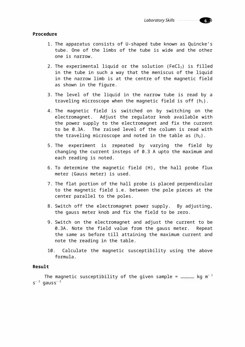
Procedure

1. The apparatus consists of U-shaped tube known as Quincke’s tube. One of the limbs of the tube is wide and the other one is narrow.

2. The experimental liquid or the solution (FeCl3) is filled in the tube in such a way that the meniscus of the liquid in the narrow limb is at the centre of the magnetic field as shown in the figure.

3. The level of the liquid in the narrow tube is read by a traveling microscope when the magnetic field is off (h1).

4. The magnetic field is switched on by switching on the electromagnet. Adjust the regulator knob available with the power supply to the electromagnet and fix the current to be 0.3A. The raised level of the column is read with the traveling microscope and noted in the table as (h2).

5. The experiment is repeated by varying the field by changing the current insteps of 0.3 A upto the maximum and each reading is noted.

6. To determine the magnetic field (H), the hall probe flux meter (Gauss meter) is used.

7. The flat portion of the hall probe is placed perpendicular to the magnetic field i.e. between the pole pieces at the center parallel to the poles.

8. Switch off the electromagnet power supply. By adjusting, the gauss meter knob and fix the field to be zero.

9. Switch on the electromagnet and adjust the current to be 0.3A. Note the field value from the gauss meter. Repeat the same as before till attaining the maximum current and note the reading in the table.

10. Calculate the magnetic susceptibility using the above formula.

Result

The magnetic susceptibility of the given sample = …………… kg m– 1 s– 2 gauss– 2

6.20

Materials Science

6.6. Dielectric Constant Measurement

Aim To determine the dielectric constant of the given sample at different temperatures.

Apparatus required The given sample, capacitance meter, dielectric sample cell, digital temperature indicator

etc.

Formula

1. The dielectric constant of the sample is given by,r = C / C0 (No unit)

where C = capacitance of the sample (farad) C0 = Capacitance of the air capacitor having the same area and

thickness as the sample (farad)

2. The capacitance of air capacitor is given by,

C0 =

ε0 Ad

( farad )

where 0 = permittivity of free space = 8.854 1012 farad / metre

A = area of the plates of the capacitor(A = r2 : r = radius of the sample)

d = thickness of the sample (or) distance between the plates (m)

Principle

The capacitance of a capacitor increases when it is filled with an insulating medium. The increase in the capacitance depends on the property of the medium, called dielectric constant (). It can be measured using either static or alternating electric fields. The static dielectric constant is measured with static fields or with low frequency ac fields. At higher frequencies, values of dielectric constant become frequency dependent. The dielectric constant varies with temperature also.

Procedure

1. The given dielectric sample inside the dielectric cell in its position without forming air gap between the plates of the sample holder.

2. Connect the thermocouple leads to a digital temperature indicator to measure the temperature of the dielectric cell

3. Also, connect the capacitance meter to the dielectric cell

4. Connect the heater terminals of the dielectric cell to ac mains through a dimmerstat.

5. At room temperature, measure the capacitance of the sample using capacitances meter.

6. Now switch on the heater and measure the capacitance of the sample at different temperature (in steps of 10°C starting from room temperature).

6.21

1000

2000

3000

4000

5000

6000

30 50 70 90 110 130 150

Temperature (Degree Celcius)

Die

lect

ric C

onst

ant

Laboratory Skills

Fig. 6.6.1 Dielectric Constant versus Temperature for barium titanate

Table 6.6.1 Determination of dielectric constant of the sample:

Sl.No. Temperature (°C) Capacitance (Farad)

Dielectric constant

(εr =CC0 )

Observation

The radius of the sample (r) = ………………….m

The thickness of the sample (d) =…………………..m

Calculation

The area of the plates of the capacitor = r2 =…….. m2

The capacitance of the air capacitor,

C =ε 0 A

d= . .. . .. .. . .. farad

6.22

Materials Science

The dielectric constant of the sample

ε n=CC0

7. Measure the thickness of the sample (d) using the micrometer screw attached in the sample cell

8. Measure the diameter of the sample using a vernier caliper and determine the radius of the sample

9. Calculate the capacitance of the air capacitor using, the relation

C0 =ε0 (πr 2)

d

10. Calculate the dielectric constant of the sample at different temperatures using the relation.

ε r = CC0

and tabulate the readings in the table

11. Plot a graph by taking temperature along X axis and dielectric constant along Y axis.

Result

The dielectric constants of the given sample at different temperature are measured and a graph is plotted between the temperature and dielectric constant.

6.23

Laboratory Skills

6.7 Calculation of Lattice Cell Parameters – X-ray Diffraction

Aim

The calculate the lattice cell parameters from the powder X-ray diffraction data.

Apparatus required

Powder X-ray diffraction diagram

Formula

For a cubic crystal1d2 =

(h2+k2+l2 )a2

For a tetragonal crystal

1d2 = {(h2+k2 )

a2 + l2

c2 }

For a orthorhombic crystal

1d2 = ( h2

a2 ) + ( k 2

b2 ) + ( l2

c2 )

The lattice parameter and interplanar distance are given for a cubic crystal as,

a = λ2 sin θ √h2+k2+l2

Å

d = a√h2+k2+ l2 Å

Where, a = Lattice parameterd = Interplanner distance

λ = Wavelength of the CuKα radiation (1.5405)h, k, l = Miller integers

Principle

Braggs law is the theoretical basis for X-ray diffraction.

(sin2 θ )hkl = ( λ2/4 a2 ) (h2+k2+l2 )

Each of the Miller indices can take values 0, 1, 2, 3, …. Thus, the factor (h2 + k2 + l2) takes the values given in Table 6.7.1.

6.24

Materials Science

Table 6.7.1 Value of h2 + k 2 + l2 for different planes

h, k, l h2 + k2 + l2 h, k, l h2 + k2 + l2

100110111200210211220221

12345689

300310311322320321400410

910111213141617

Fig.6.7.1 XRD pattern

The problem of indexing lies in fixing the correct value of a by inspection of the sin2 values.

Procedure:

From the 2 values on a powder photograph, the values are obtained. The sin2 values are

tabulated. From that the values of

1 × sin2θsin2θmin

,

2 × sin2 θsin2 θmin

,

3 × sin2θsin2θmin

are determined and are

tabulated. The values of

3 × sin2θsin2θmin

are rounded to the nearest integer. This gives the value of h2+k2+l .From these the values of h,k,l are determined from the Table.6.7.1.

From the h,k,l values, the lattice parameters are calculated using the relation

a = λ2 sin θ √h2+k2+l2

Å

d = a√h2+k2+ l2 Å

2

Inte

nsity

6.25

Laboratory Skills

Table 6.7.2 Value of h2 + k 2 + l2 for different planes

S. No 2 sin2 1 × sin2 θsin2 θmin

2 × sin2 θsin2 θmin

3 × sin2θsin2θmin

h2+k2+l2 hkl aÅ

dÅ

Table 6.7.3 Lattice determination

Lattice type Rule for reflection to be observed

Primitive P

Body centered I

Face centered F

None

hkl : h + k + l = 2 n

hkl : h, k, l either all odd or all even

Depending on the nature of the h,k,l values the lattice type can be determined.

Result:

The lattice parameters are calculated theoretically from the powder x-ray diffraction pattern.

6.26

Power supply IR source

Sample holder Photo-diode

Micro controllerDisplay device

Sensing circuit

Materials Science

6.8 Determination of Glucose Concentration using Sensor

Aim

To determine the glucose concentration in the solutions of different concentration using IR sensor.

Apparatus required

Infra red LED, Photodiode, Amplification circuit board, Microcontroller board of 16F877A , LCD, Power supply, Test Tube, Glucose – various concentrations like 10mg, 20mg, 30mg etc.

Principle

In this non invasive method, the infra red source and the detector work on the principle of transmission mode. Test tube with various glucose concentrations are placed in between an infrared light emitting diode and the photodiode. The infrared light source is transmitted through the test tube where there will be a change in optical properties of the light. Now the transmitted light is detected by the photodiode, which converts the light into electrical signal. This signal is sent to the microcontroller and output is displayed in the LCD.The experiment is repeated with different concentrations of glucose solutions and a graph is plotted between glucose concentration and voltage as indicated in Fig.6.8.2.

Fig.6.8.1 Schematic representation for determining glucose concentration

Fig.6.8.2 Variation of voltage with glucose concentration

Glucose concentration

Vol

tage

6.27

Laboratory Skills

Table 6.8.1 Variation of voltage with glucose concentration

S.No Glucose concentrations (mg)

Voltage obtained (V)

Result

The glucose concentrations have been determined and the variations of voltage with glucose concentration have been plotted.

6.28