Embed Size (px)
Citation preview

Natio al I dustrial Competitive ess through E ergy, E viro me t a d Eco omics NICE 3 Gra t No. DE-FG48-96R8-10598
Adva ced Process A alysis for Source Reductio i the Sulfuric Acid Petroleum Refi i g Alkylatio Process
Fi al Tech ical Report
by
Michael K. Rich Motiva E terprises
David McGee Louisia a Departme t of Natural Resources
Jack R. Hopper a d Carl L. Yaws Lamar U iversity
Derya B. Özyurt a d Ralph W. Pike Louisia a State U iversity
A joi t project with Louisia a Departme t of Natural Resources,
Motiva E terprises, a d Gulf Coast Hazardous Substa ce Research Ce ter
submitted to the
U. S. Departme t of E ergy
September 1, 2001
Gulf Coast Hazardous Substa ce Research Ce ter Lamar U iversity
Beaumo t, Texas 77710

TABLE F C NTENTS
ABSTRACT v
LIST OF TABLES vi
LIST OF FIGURES vii
CHAPTER 1. INTRODUCTION 1 Overview of Adva ced Process A alysis System 1 Flowsheet Simulatio 3 O -Li e Optimizatio 4 Chemical Reactor A alysis 6 Pi ch A alysis 7 Pollutio Assessme t 9 Alkylatio 10 Summary 11
CHAPTER 2. LITERATURE REVIEW 12
Reactio Mecha ism for Alkylatio of Isobuta e
Reactio Mecha ism for Alkylatio of Isobuta e
Adva ced Process A alysis System 12 I dustrial Applicatio s of O -Li e Optimizatio 13 Key Eleme ts of O -Li e Optimizatio 14 E ergy Co servatio 15 Pollutio Preve tio 16
Sulfuric Acid Alkylatio Process 22 Alkylatio i Petroleum I dustry 23 Commercial Sulfuric Acid Alkylatio Process 24 Theory of Alkylatio Reactio s 26
with Propyle e 30
with Butyle e a d Pe tyle e 30 I flue ce of Process Variables 34 Feedstock 36 Products 36 Catalysts 37
Summary 38
CHAPTER 3. METHODOLOGY 39 Flowsheeti g Program 40 O -Li e Optimizatio Program 43 Chemical Reactor A alysis Program 47 Heat Excha ger Network Program 48 Pollutio I dex Program 51 Summary 53
ii
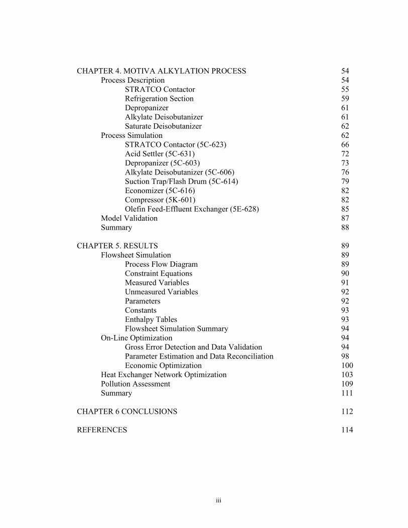
CHAPTER 4. MOTIVA ALKYLATION PROCESS 54 Process Descriptio 54
STRATCO Co tactor 55 Refrigeratio Sectio 59 Depropa izer 61 Alkylate Deisobuta izer 61 Saturate Deisobuta izer 62
Process Simulatio 62 STRATCO Co tactor (5C-623) 66 Acid Settler (5C-631) 72 Depropa izer (5C-603) 73 Alkylate Deisobuta izer (5C-606) 76 Suctio Trap/Flash Drum (5C-614) 79 Eco omizer (5C-616) 82 Compressor (5K-601) 82 Olefi Feed-Efflue t Excha ger (5E-628) 85
Model Validatio 87 Summary 88
CHAPTER 5. RESULTS 89 Flowsheet Simulatio 89
Process Flow Diagram 89 Co strai t Equatio s 90 Measured Variables 91 U measured Variables 92 Parameters 92 Co sta ts 93 E thalpy Tables 93 Flowsheet Simulatio Summary 94
O -Li e Optimizatio 94 Gross Error Detectio a d Data Validatio 94 Parameter Estimatio a d Data Reco ciliatio 98 Eco omic Optimizatio 100
Heat Excha ger Network Optimizatio 103 Pollutio Assessme t 109 Summary 111
CHAPTER 6 CONCLUSIONS 112
REFERENCES 114
iii

APPENDICES A ESTIMATION OF CONCENTRATIONS IN VARIOUS
SPECIES IN THE CATALYST PHASE A-1
B MODEL EQUATIONS (EQUALITY AND INEQUALITY CONSTRAINTS) A-13
C INPUT TO FLOWSHEET SIMULATION A-61 C.1 List of process u its A-63 C.2 List of process streams A-65 C.3 Measured values (i itial poi ts) A-69 C.4 U measured variables (i itial poi ts) A-72 C.5 Parameters A-105 C.6 Coefficie t values to calculate the e thalpy of gas phase A-107 C.7 Coefficie t values to calculate the e thalpy of liquid phase A-108 C.8 Co sta ts A-109
D OUTPUT FROM ON-LINE OPTIMIZATION A-111 D.1 Measured Variables A-111 D.2 U measured Variables A-129 D.3 Pla t Parameters A-331
E LIST OF STREAMS FROM THE ALKYLATION PROCESS MODEL USED FOR PINCH ANALYSIS A-343
F OUTPUT OF THE THEN PROGRAM A-345
G SEIP VALUES OF THE COMPONENTS IN THE ALKYLATION PROCESS A-351
H PROGRAM OUTPUTS A-352 H.1 Data Validatio Program (Do_data.lst) A-352 H.2 Parameter Estimatio Program (Do_para.lst) A-614 H.3 Eco omic Optimizatio Program (Do_eco .lst) A-881
I CALCULATION OF THE STEADY STATE OPERATION POINTS A-1141
J USER’S MANUAL A-1143
iv

ABSTRACT
Advanced Process Analysis System was successfully applied to the 15,000 BPD
alkylation plant at the Motiva Enterprises Refinery in Convent, Louisiana. Using the
flowsheeting, on-line optimization, pinch analysis and pollution assessment capabilities
of the Advanced Process Analysis System an average increase in the profit of 127% can
be achieved. Energy savings attained through reduced steam usage in the distillation
columns total an average of 9.4x10⁹ BTU/yr. A maximum reduction of 8.7% (67x109
BTU/yr) in heating and 6.0% (106x109 BTU/yr) in cooling requirements is shown to be
obtainable through pinch analysis. Also one of the main sources of the pollution from
the alkylation process, sulfuric acid consumption, can be reduced by 2.2 %.
Besides economic savings and waste reductions for the alkylation process,
which is one of the most important refinery processes for producing conventional
gasoline, the capabilities of an integrated system to facilitate the modeling and
optimization of the process has been demonstrated. Application to other processes could
generate comparable benefits.
The alkylation plant model had 1,579 equality constraints for material and
energy balances, rate equations and equilibrium relations. There were 50 inequality
constraints mainly accounting for the thermodynamic feasibility of the system. The
equality and inequality constraints described 76 process units and 110 streams in the
plant. Verification that the simulation described the performance of the plant was shown
using data validation with 125 plant measurements from the distributed control system.
There were 1,509 unmeasured variables and 64 parameters in the model.
v

List of Tables
Table 2.1. Ψsk,l Values used in Alkylation Process Model 20
Table 2.2 Reaction Mechanism and Material Balances for Sulfuric Acid Alkylation of Isobutane with Propylene 32
Table 2.3 Reaction Mechanism and Material Balances for Sulfuric Acid Alkylation of Isobutane with Butylene 33
Table 4.1 Summary of the contractor model (5C-623) 71
Table 4.2 Summary of the acid settler model (5C-631) 72
Table 4.3 Summary of the depropanizer model (5C-603) 75
Table 4.4 Summary of the deisobutanizer model (5C-606A) 77
Table 4.5 Summary of the suction trap/flash drum model (5C-614) 81
Table 4.6 Summary of the compressor model (5K-601) 85
Table 4.7 Summary of the exchanger model (5E-628) 86
Table 4.8 Plant vs. Model Data 87
Table 5.1 Summary of Alkylation Model 94
Table 5.2 Measured Variables for operation point #1 95
Table 5.3 Plant Parameters for operation point #1 99
Table 5.4 Alkylation Plant Raw Material/Utility Costs and Product Prices 102
Table 5.5 Calculated Profit after Data Validation (D.V.),
Parameter Estimation (P.E.) and Economic Optimization (E.O.)
Steps for six Different Operation Points (Steady States) 103
Table 5.6 Input and Output Streams in Alkylation Process 109
Table 5.7. Pollution Assessment Values for Alkylation Process
before (BEO) and after (AEO) the economic optimization. 110
vi

List of Figures
Figure 1.1 Framework of Advanced Process Analysis System 2
Figure 1.2 Simplified Structure of On-Line Optimization 5
Figure 1.3 Reactor Design Program Outline 6
Figure 1.4 Composite Curves for Hot Streams and Cold Streams 8
Figure 1.5 Grid Diagram 8
Figure 2.1 Relationship between key elements of on-line optimization 15
Figure 2.2 Sulfuric Acid Alkylation Process (Vichailak 1995) 24
Figure 2.3 STRATCO Effluent Refrigeration Reactor (Yongkeat, 1996) 25
Figure 3.1 ‘Onion Skin’ Diagram for Organization of a Chemical
Process and Hierarchy of Analysis 39
Figure 3.2 Example of Flowsim Screen for a Simple Refinery 42
Figure 4.1 Reactor and Refrigeration Sections of Alkylation Process 56
Figure 4.2 Depropanizer and Alkylate Deisobutanizer Sections of
Alkylation Process 57
Figure 4.3 Saturate Deisobutanizer Section of Alkylation Process 58
Figure 4.4 STRATCO Effluent Refrigeration Reactor 59
Figure 4.5 Process flow diagram, as developed with the Flowsheet
Simulation tool of Advanced Process Analysis System 65
Figure 4.6 Contactor 5C-623 66
Figure 4.7 Suction Trap Flash Drum (5C-614) 79
Figure 4.8 Economizer (5C-616) 82
Figure 4.9 Compressor (5K-601) 84
Figure 5.1 Grand Composite Curve for Alkylation Process 105
vii

Figure 5.2 Network Grid Diagram for Alkylation Process 107
Figure 5.3 Integrating columns (5C-601 and 5C-603) with the process:
Pressure shift for column 5C-601 only (left),
for both columns (right). 108
viii

CHAPTE 1
INT ODUCTION
This epo t documents the esults of applying the Advanced P ocess Analysis
System fo ene gy conse vation and pollution eduction in a comme cial, sulfu ic acid
catalyzed, alkylation plant at the Motiva Ente p ises Refine y in Convent, Louisiana.
The Advanced P ocess Analysis System was developed fo use by p ocess and plant
enginee s to pe fo m comp ehensive evaluations of p ojects in depth significantly
beyond thei cu ent capabilities. The st ategy has the advanced p ocess analysis
methodology identify sou ces of excess ene gy use and of pollutant gene ation. This
p og am has built on esults f om esea ch on sou ce eduction th ough technology
modification in eactions and sepa ations, ene gy conse vation (pinch analysis) and on-
line optimization (p ocess cont ol) by P ofesso s Hoppe and Yaws at Lama and
P ofesso Pike at Louisiana State Unive sity. The System uses the Lama chemical
eacto analysis p og am, the LSU on-line optimization and pinch analysis p og ams,
and the EPA pollution index methodology. Visual Basic was used to integ ate the
p og ams and develop an inte active Windows inte face whe e info mation is sha ed
th ough the Access database. This chapte gives an ove view of Advanced P ocess
Analysis System and an int oduction to the alkylation p ocess. These a e desc ibed in
g eate detail subsequent chapte s.
1.1 Overview of the Advanced Process Analysis System
The advanced p ocess analysis methodology identifies sou ces of excess ene gy
use and of pollutant gene ation was based on the f amewo k shown in Figu e 1.1. The
main components of this system a e flowsheet simulation, on-line optimization, eacto
analysis, pinch analysis, and pollution assessment. The flowsheet simulation p og am is
used
1

Pollution Index
Advanced Process Analysis System
On-Line Optimization
eactor Analysis
Pinch Analysis
Process Control
Process Modification
Flowsheet Simulation
Process pecification :
PFD, units, streams, physical properties
Key word index: Unit ID, tream ID, Component ID, Property ID
DataBase of APA :
PFD: units & streams Unit : local variables
parameters balance equations stream connection
treams: global variables Plant data Property: enthalpy function
density, viscosity
F : simulation data
OLO: optimal setpoints reconciled data estimated parameters
RA: reactor comparison best reactor for the process
PA: best heat exchanger network
PI: pollution information
On-Line Optimization
Reactor Analysis
Pinch Analysis
Pollution Index
Units, streams, physical property
imulation data
Units, streams, physical property plant data
Optimal setpoints, reconciled data, parameters
Temp., flow rates enthalpy function
Reactor comparison
Best heat exchanger network
Flow rates, composition
Temp., flow rates enthalpy function
Pollution information
Flowsheet imulation
Figu e 1.1: F amewo k of Advanced P ocess Analysis System
2

fo p ocess mate ial and ene gy balances. Online optimization gives an accu ate
desc iption of the chemical o efine y p ocess being evaluated. This p ocess
simulation is used fo offline studies using eacto analysis, pinch analysis and pollution
assessment, to achieve p ocess imp ovements that educe pollution and ene gy
consumption.
The Advanced P ocess Analysis System has been applied to two contact
p ocesses at the IMC Ag ico Company’s ag icultu al chemical complex. The esults of
the application of the System showed a potential annual inc ease in p ofit of 3% (o
$350,000) and a 10% eduction in sulfu dioxide emissions ove cu ent ope ating
conditions using the on-line optimization component of the System. The chemical
eacto analysis component showed that the eacto conve sion could be inc eased by
19% and that the eacto volume dec eased by 87% by using a eacto p essu e of 10.3
atm athe than the cu ent 1.3 atm. The pinch analysis component showed that the
minimum amount of cooling wate was being used, and the heat exchange netwo k
could be econfigu ed to educe the numbe of heat exchange s being used and educe
the total heat exchange a ea by 25%. The pollution assessment component of the
System identified the sulfu fu nace and conve te s as the pa ts of the p ocess to be
modified to minimize emissions. Details of these esults we e given in the thesis of
Keda Telang, 1998.
1.2 Flowsheet Simulation
The flowsheet simulation, Flowsim, is used to develop the p ocess model, and it
has a g aphical use inte face with inte active capabilities. P ocess units a e ep esented
as ectangula shapes whe eas the p ocess st eams a e ep esented as lines with a ows
between these units. Each p ocess unit and st eam included in the flowsheet must have a
3
name and a desc iption. P ocess info mation is divided into the following six catego ies:
equality const aints, inequality const aints, unmeasu ed va iables, measu ed va iables,
pa amete s and constants. All of this p ocess info mation is ente ed with the help of the
inte active, use -customized g aphic sc eens of Flowsim, and the info mation is sto ed
in an Access database fo use by the othe p og ams.
The info mation in the fi st five catego ies is fu the classified by associating it
with eithe a unit o a st eam in the flowsheet. Fo example, fo a unit that is a heat
exchange , the elevant info mation includes the mass balance and heat t ansfe
equations, limitations on the flow ates and tempe atu es if any, the heat t ansfe
coefficient pa amete and all the inte mediate va iables defined fo that exchange .
Fo a st eam, the info mation includes its tempe atu e, p essu e, total flow ate,
mola flow ates of individual components etc. Also, info mation not linked to any one
unit o st eam is called the ‘Global Data’. Fo example, the ove all daily p ofit of the
p ocess is aglobal unmeasu ed va iable.
The fo mulation of p ocess model fo the alkylation p ocess is desc ibed in
detail in the use s’ manual in Appendix J. The on-line optimization p og am uses the
p ocess model as const aint equations to maintain the p ocess ope ating at optimal set
points in the dist ibuted cont ol system
1.3 On-line Optimization
Online optimization is the use of an automated system which adjusts the
ope ation of a plant based on p oduct scheduling and p oduction cont ol to maximize
p ofit and minimize emissions by p oviding setpoints to the dist ibuted cont ol system.
This is illust ated in Figu e 1.2. Plant data is sampled f om the dist ibuted cont ol
system, and g oss e o s a e emoved f om it. Then, the data is econciled to be
4

consistent with the mate ial and ene gy balances of the p ocess. An economic model is
used to compute the p ofit fo the plant and the plant model is used to dete mine the
ope ating conditions, e.g. tempe atu es, p essu es, flow ates of the va ious st eams.
These a e va iables in the mate ial and ene gy balance of the plant model. The plant and
economic model a e togethe used with an optimization algo ithm to dete mine the best
ope ating conditions (e.g. tempe atu es, p essu es etc.) which maximizes the p ofit.
These optimal ope ating conditions a e then sent to the dist ibuted cont ol system to
p ovide setpoints fo the cont olle s.
Figu e 1.2: Simplified St uctu e of Online Optimization
Gross Error Detection and
Data Reconcilation
Optimization Algorithm Economic Model Plant Model
data
plant measurements
setpoints for
controllers
optimal operating conditions
reconciled
plant model parameters
Distributed Control ystem
sampled
plant data
Plant Model Parameter Estimation
setpoint targets
economic model parameters
5

1.4 Chemical eactor Analysis
The Chemical Reacto Analysis p og am is a comp ehensive, inte active
compute simulation fo th ee-phase catalytic gas-liquid eacto s and thei subsets, and
an outline is shown in Figu e 1.3. The p og am has been developed by P ofesso
Hoppe and his esea ch g oup at Lama Unive sity (Saleh et al., 1995). It has a wide
ange of applications such as oxidation, hyd ogenation, hyd odesulfu ization,
hyd oc acking and Fische -T opsch synthesis. This p og am inte actively guides the
enginee to select the best eacto design fo the eacting system based on the
cha acte istics of ten diffe ent types of indust ial catalytic gas-liquid eacto s which
includes catalyst pa ticle diamete and loading, diffusivities, flow egimes, gas-liquid
and liquid-solid mass t ansfe ates, gas and liquid dispe sions, heat t ansfe , holdup
among othe s. The p og am solves the conse vation equations and has checks fo the
validity of the design, e.g., not allowing a complete catalyst-wetting facto if the liquid
flow ate is not sufficient. A mo e detailed desc iption is in the use 's manual.
Reaction
Homogeneous Hete ogeneous
Gas Phase Liquid Phase Catalytic
PFR CSTR
Gas-Liquid
Gas Liquid Gas-Liquid CSTR Bubble Reacto Packed Bed
Batch Reacto Fixed Bed Reacto T ickle Bed
Fluidised Bed Reacto Fixed Bubble Bed CSTR Slu y Bubble Slu y
3-Phase Fluidised Bed
Figu e 1.3: The Reacto Design P og am Outline
6

1.5 Pinch Analysis
Pinch technology was developed in the late 1970's as a method fo the design of
heat exchange netwo ks, and it has since been extended to site ene gy integ ation
including distillation and utility systems, mass exchange s, and a numbe of othe
applications (Linnhoff, 1993; Gupta and Manousiouthakis, 1993). Pinch analysis
dete mines the best design fo sepa ations, ecycle and heat exchange netwo ks. It
employs th ee concepts: the composite cu ves, the g id diag am of p ocess st eams and
the pinch point; and these a e applied to minimize ene gy use in the p ocess.
Illust ations of composite cu ves and the g id diag am a e shown in Figu e 1.4 and
Figu e 1.5 espectively. The composite cu ves a e plots of tempe atu e as a function of
enthalpy f om the mate ial and ene gy balances fo the st eams that need to be heated,
called cold st eams, and those that need to be cooled, called hot st eams. F om the
composite cu ves of the hot and cold st eams, the potential fo ene gy exchange
between the hot and cold st eams can be dete mined, as well as the p ocess
equi ements fo exte nal heating and cooling f om utilities such as steam and cooling
wate . At one o mo e points the cu ves fo the hot and cold st eams may come ve y
close, the p ocess pinch; and this means the e is no su plus heat fo use at lowe
tempe atu es. The g id diag am has ve tical lines to ep esent the hot and cold st eams
with lengths co esponding to the tempe atu e ange with the hot st eams going f om
top left and the cold st eams f om bottom ight. With this a angement the heat
ecove y netwo k fo the p ocess design can be dete mined. A g and composite,
tempe atu e-enthalpy cu ve can be assembled f om the composite cu ves and the g id
diag am to help select utilities and app op iately place boile s, tu bines, distillation
columns, evapo ato s and fu naces. Also, the heat t ansfe su face a ea can be
7

dete mined with the co esponding capital cost fo both ene gy and cost minimization.
This methodology is inco po ated in compute p og am THEN which is inco po ated in
the Advanced P ocess Analysis System.
0
40
80
120
160
0 100 200 300 400 500
Q (W)
T (°C)
H1+H2
0
40
80
120
160
0 100 200 300 400 500
Q (W)
T (°C) C1+C2
Figu e 1.4: Composite Cu ves fo Hot St eams (on the left side) and Cold St eams (on the ight side) fo the Simple P ocess
4
3
2
1 1
2
H1
H2
C1
C2
Heate Coole Loop
1
2
Heat Exchange
Figu e 1.5: G id Diag am
in selecting utilities and app op iate placement of boile s, tu bines, distillation columns,
evapo ato s and fu naces.
8
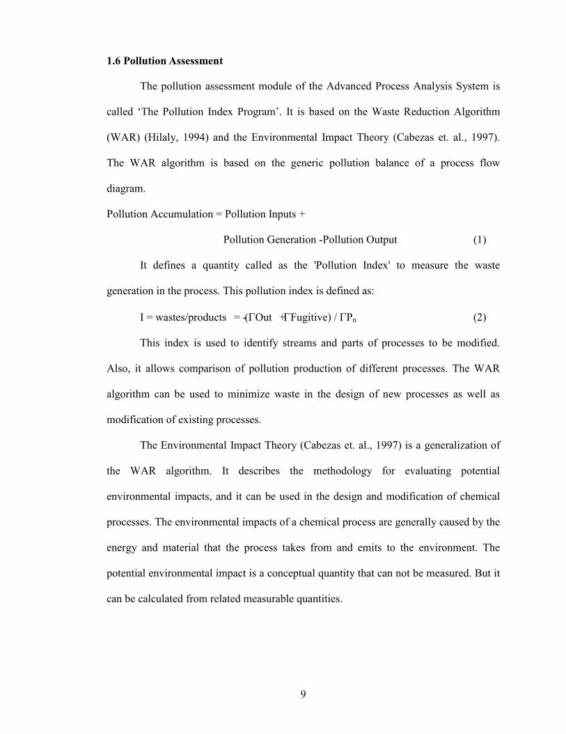
1.6 Pollution Assessment
The pollution assessment module of the Advanced P ocess Analysis System is
called ‘The Pollution Index P og am’. It is based on the Waste Reduction Algo ithm
(WAR) (Hilaly, 1994) and the Envi onmental Impact Theo y (Cabezas et. al., 1997).
The WAR algo ithm is based on the gene ic pollution balance of a p ocess flow
diag am.
Pollution Accumulation = Pollution Inputs +
Pollution Gene ation -Pollution Output (1)
It defines a quantity called as the 'Pollution Index' to measu e the waste
gene ation in the p ocess. This pollution index is defined as:
I = wastes/p oducts = -(ΓOut +ΓFugitive) / ΓPn (2)
This index is used to identify st eams and pa ts of p ocesses to be modified.
Also, it allows compa ison of pollution p oduction of diffe ent p ocesses. The WAR
algo ithm can be used to minimize waste in the design of new p ocesses as well as
modification of existing p ocesses.
The Envi onmental Impact Theo y (Cabezas et. al., 1997) is a gene alization of
the WAR algo ithm. It desc ibes the methodology fo evaluating potential
envi onmental impacts, and it can be used in the design and modification of chemical
p ocesses. The envi onmental impacts of a chemical p ocess a e gene ally caused by the
ene gy and mate ial that the p ocess takes f om and emits to the envi onment. The
potential envi onmental impact is a conceptual quantity that can not be measu ed. But it
can be calculated f om elated measu able quantities.
9

1.7 Alkylation
Alkylation is an impo tant pet oleum efining p ocess that is used to conve t
light isopa affins and light olefins into high octane numbe isopa affins. Isopa affins
containing a te tia y ca bon atom unde go catalytic alkylation with C3-C5 olefins to
p oduce highly b anched pa affins in the C7-C9 ange. This involves a composite of
consecutive and simultaneous eactions including polyme ization, disp opo tionation,
c acking and self-alkylation eactions (Co ma and Ma tinez, 1993). Comme cially,
isobutane is used fo the p ocess because isopentane and highe isopa affins have octane
numbe s that a e quite desi able.
Catalytic alkylation occu s in the p esence of sulfu ic (H2SO4) o hyd ofluo ic
acid (HF) catalysts, at mild tempe atu es and at sufficient p essu e to maintain the
hyd oca bons in the liquid state. With sulfu ic acid it is necessa y to ca y out the
eactions at 10 to 20°C (50 to 70°F) o lowe , to minimize oxidation- eduction
eactions, which esult in fo mation of ta s and p oduction of sulfu dioxide. When
hyd ofluo ic acid is the catalyst, eaction tempe atu e is usually limited to 35°C (100°F)
o lowe . The catalyst exists as a sepa ate phase, and the eactants and p oducts must be
t ansfe ed to and f om the catalyst (G use and Stevens 1960, Rosenwald 1978).
Comme cial alkylation plants use eithe sulfu ic acid (H2SO4) o hyd ofluo ic
acid (HF) as catalysts. About 20 yea s ago almost th ee times as much alkylate was
p oduced using H2SO4 as the catalyst as compa ed to p ocesses using HF. Since then the
elative impo tance of p ocesses using HF has inc eased substantially and cu ently
these p ocesses p oduce in the U.S. about 47% of the alkylate. Howeve , in the last five
yea s, mo e H2SO4 than HF type units have been built due to envi onmental and safety
conce ns. Recent info mation cla ifying the dange s of HF is causing efine ies that use
10

HF to econside the catalyst, o imp ove the safety of equipment and p ocedu es
(Alb ight 1990a, Cupit et al. 1961).
1.8 Summary
An ove view of the Advanced P ocess Analysis System was given and
successful applications to othe p ocesses we e desc ibed b iefly. Also, the cu ent
status of comme cial alkylation p ocesses was given.
In the next chapte a lite atu e su vey is given on cu ent status of the techniques
inco po ated in the Advanced P ocess Analysis System and alkylation p ocess chemist y
and ope ations. The thi d chapte of this epo t desc ibes the application of the
Advanced P ocess Analysis System to the alkylation p ocess. The fou th chapte gives
the desc iption of the development of the p ocess model of the alkylation p ocess using
Advanced P ocess Analysis System. The fifth chapte p esents the esults of the analysis
fo the p ocess.
11

�
CHAPTE 2��
LITE ATU E EVIEW
In�t is�c apter� t e�current�status�of� t e�met odology�and�literature�is�reviewed�
for� t e� met ods� used� in� t e� Advanced� Process� Analysis� System.� Also� t e� current�
understanding�of�t e�alkylation�process�and�its�tec nology�is�given.��
2.1 Advanced Process Analysis System
� Advanced� Process� Analysis� System,� based� on� t e� framework� given� in� Figure�
1.1,�includes�c emical�reactor�analysis,�process�flows eeting,�pinc �analysis�and�on!line�
optimization.� All� of� t ese� programs� use� t e� same� information� of� c emical� processes��
(material�and�energy�balances,�rate�equations�and�equilibrium�relations).��Consequently,�
an�advanced�and�integrated�approac �for�process�analysis�is�available�now.�
� T e�need�of�an�integrated�approac �to�process�analysis� as�been�given�by�Van�
Reeuwijk� et� al.� (1993)� w o� proposed� aving� a� team� of� computer� aided� process�
engineering� expert� and� a� process� engineer� wit � tec nology� knowledge� to� develop�
energy� efficient� c emical� processes.� A� process� engineer� software� environment� is�
described�by�Ballinger�et�al.�(1994)�called�‘epee’�w ose�goal�is� ave�to�a�user�interface�
to� create� and� manipulate� objects� suc � as� processes,� streams� and� components� wit �
s aring� of� data� among� process� engineering� applications� in� an� open� distributed�
environment.�T e�Clean�Process�Advisory�System�(CPAS)� as�been�described�by�Baker�
et� al.(1995)� as� a� computer� based� pollution� prevention� process� and� product� design�
system�t at�contains�ten�PC�software�tools�being�developed�by�an�industry!government!
university� team.� �T is� includes� tec nology�selection�and�sizing,�potential�and�designs,�
p ysical� property� data,� materials� locators� and� regulatory� guidance� information.� An�
article� by� S aney� (1995)� describes� t e� various� modeling� software� and� databases�
12�

�
available� for� process� analysis� and� design.� A� review� of� computer� aided� process�
engineering�by�Winter�(1992)�predicts�linking�various�applications�will�result�in�better�
quality� of� process� design,� better� plant� operations� and� increased� productivity.� It� also�
describes� t e� PRODABAS� concept,� w ic � focuses� on� capturing� information� from�
multiple�sources� into�a�common�multi!user� framework�for�analysis,�process�definition�
and�process� engineering�documentation� rat er� t an� t e�original� concept�of� a� common�
user�interface�and�datastore�linked�wit �a�range�of�applications�computing�tools.�
2.1.1 Industrial Applications of On-Line Optimization
� Boston,� et� al.,� (1993)� gave� a� wide� review� of� computer� simulation� and�
optimization�as�well�as�advanced�control� in�c emical�process� industries.�He�described�
t e� new� computing� power� for� process� optimization� and� control� t at� leads� to� ig er�
product�qualities�and�better�processes,�w ic �are�cleaner,�safer,�more�efficient,�and�less�
costly.�
� Lauks,�et�al.,�(1992)�reviewed�t e�industrial�applications�of�on!line�optimization�
reported�in�t e�literature�from�1983�to�1991�and�cited�nine�applications�–�five�et ylene�
plants,� a� refinery,�a�gas�plant,� a�crude�unit� and�a�power� station.�T e� results� s owed�a�
profitability� increase� of� 3%� or� $4M/year.� Also,� intangible� profits� from� a� better�
understanding�of�plant�be avior�were�significant.�
� Z ang�(1993)�conducted�a�study�of�on!line�optimization�for�Monsanto!�designed�
sulfuric� acid� plant� of� IMC� Agrico� at� Convent,� Louisiana.� Economic� optimization� can�
ac ieve� a�17%� increase� in�plant�profit� and�25%� reduction� in� sulfur�dioxide� emission.�
T e�plant�was�studied�by�C en�(1998),� in�developing� t e�optimal�way� to�conduct�on!
13�

�
line�optimization.�Also,�C en�(1998)�reported�a�number�of�ot er�successful�applications�
of�on!line�optimization�in�improving�c emical�processes.�
2.1.2 Key Elements of On-Line Optimization
� T e�objective�of�on!line�optimization�is� to�determine�optimal�process�setpoints�
based�on�plant’s� current�operating� and�economic� conditions.�As� s own� in�Figure�1.2,�
t e�key�elements�of�on!line�optimizations�are�(C en,�1998):�
! Gross�Error�Detection�
! Data�Reconciliation�
! Parameter�Estimation�
! Economic�Model�(Profit�Function)�
! Plant�Model�(Process�Simulation)�
! Optimization�Algorit m�
T e� procedure� for� implementing� on!line� optimization� involves� steady!state� detection,�
data�validation,�parameter�estimation,�and�economic�optimization.�
� T e� relations ip� between� t ese� key� elements� is� outlined� in� Figure� 2.1.� Bot �
plant� model� and� optimization� algorit ms� are� required� in� t e� t ree� steps� of� on!line�
optimization�–�data�validation,�parameter�estimation,�and�economic�optimization.�Plant�
model� serves� as� constraint� equations� in� t e� t ree� nonlinear� optimization� problems,�
w ic � are� solved� by� t e� optimization� algorit m.� For� data� validation,� errors� in� plant�
measurements�are�rectified�by�optimizing�a�likeli ood�function�subject�to�plant�model,�
and� a� test� statistic� is� used� to� detect� gross� errors� in� t e� measurements.� For� parameter�
estimation,� parameters� in� plant� model� are� estimated� by� optimizing� an� objective�
function,� suc � as� minimizing� t e� sum� of� squares� of� measurement� errors,� subject� to�
14�

�
constraints�in�t e�plant�model.�For�economic�optimization,�t e�plant�model�is�used�wit �
economic� model� to� maximize� plant� profit� and� provide� optimal� setpoints� for� t e�
distributed�control�system�to�operate.�
�
� Figure�2.1�Relations ip�between�key�elements�of�on!line�optimization�
2.1.3 Energy Conservation
Heat�Exc anger�Network�Synt esis�(HENS)�for�maximum� eat�recovery� is� t e�
key�to�energy�conservation�in�a�c emical�plant.�T e�problem�of�design�and�optimization�
of� eat� exc anger� networks� as� received� considerable� attention� over� t e� last� two�
decades�(A mad�et�al.,�1990,�Duran�et�al.,�1986,�Lin off�et�al.�1978,�1979,�1982).��
T e�problem�of�HENS�can�be�defined�as� t e�determination�of� a� cost!effective�
network� to� exc ange� eat� among� a� set� of� process� streams� w ere� any� eating� and�
cooling� t at� is� not� satisfied� by� exc ange� among� t ese� streams� must� be� provided� by�
external�utilities�(S enoy,�1995).�Attempts�at�solving�t is�problem� ave�been�based�on�
t e�following�approac es.�
Heuristic Approaches:�T e�HENS�problem�was�first�formulated�by�Masso�and�
Rudd� (1969).� At� t at� time,� t e� design� met ods� were� generally� based� on� euristic�
15�

�
approac es.�One�of�t e�commonly�used�rules�was�to�matc �t e� ottest�stream�wit �t e�
coldest�stream.�Several�ot er�met ods�were�based�on�tree�searc �tec niques�(Lee�et�al.,�
1970).�T is�generally�led�to�feasible�but�non!optimal�solutions.�
Pinch Analysis: Ho mann� (1971)� made� significant� contributions� to� t e�
development� of� t e� t ermodynamic� approac .� In� t e� late� 1970s,� Linn off� and�
Hindmars �(Linn off�et�al.,�1979)� first� introduced�Pinc �Analysis;�a�met od�based�on�
t ermodynamic�principles.�T ey�also�introduced�a�number�of�important concepts, w ic �
formed�t e�basis�for�furt er�researc .�T ese�concepts�were�reviewed�by�Gundersen�et�al.�
(1987),�and�summarized�by�Telang�(1998).�
Mathematical Programming: Developments� in� computer� ardware� and�
software� enabled� t e� development� of� met ods� based� on� mat ematical� programming.�
Paoulias�and�Grossman�(1983)�formulated�Maximum�Energy�Recovery�(MER)�problem�
as�a�linear�programming�(LP)�model�based�on�t e�transs ipment�model,�w ic �is�widely�
used�in�operations�researc .�T is�model�was�expanded�to�make�restricted� ot�and�cold�
stream�matc es�by�using�mixed�integer�linear�programming�(MILP)�formulation.���
� HEXTRAN,�SUPERTARGET�and�ASPEN�PINCH�are�some�of� t e�commonly�
used�commercial� eat�exc anger�design�programs.�
2.1.4 Pollution Prevention
� Cost� minimization� as� traditionally� been� t e� objective� of� c emical� process�
design.�However,�growing�environmental�awareness�now�demands�process�tec nologies�
t at� minimize� or� prevent� production� of� wastes.� T e� most� important� issue� in�
development� of� suc � tec nologies� is� a� met od� to� provide� a� quantitative� measure� of�
waste�production�in�a�process.��
16�

�
Waste eduction Algorithm:�Many�different�approac es�(Telang,�1998)� ave�
been� suggested� to� deal� wit � t is� problem.� One� of� t ese� is� t e� Waste� Reduction�
Algorit m�(WAR)�(Hilaly,�1994).�T e�WAR�algorit m�is�based�on�t e�generic�pollution�
balance�of�a�process�flow�diagram.�
Pollution�Accumulation�=�Pollution�Inputs�+�� ������Pollution�Generation�!�Pollution�Output� � � (2.1)�
� It� defines� a� quantity� called� as� t e� 'Pollution� Index'� to� measure� t e� waste�
generation�in�t e�process.�T is�pollution�index�is�defined�as:�
I�=�wastes/products�=�!�(ΓOut�+�ΓFugitive)�/�ΓPn� � � (2.2)�
T is� index� is� used� to� identify� streams� and� parts� of� processes� to� be� modified.�
Also,� it� allows� comparison� of� pollution� production� of� different� processes.� T e� WAR�
algorit m� can� be� used� to� minimize� waste� in� t e� design� of� new� processes� as� well� as�
modification�of�existing�processes.�
Environmental Impact Theory: T is� t eory� (Cabezas� et.� al.,� 1997)� is� a�
generalization� of� t e� WAR� algorit m.� It� describes� t e� met odology� for� evaluating�
potential�environmental� impacts,�and� it� can�be�used� in� t e�design�and�modification�of�
c emical� processes.� T e� environmental� impacts� of� a� c emical� process� are� generally�
caused� by� t e� energy� and� material� t at� t e� process� takes� from� and� emits� to� t e�
environment.��T e�potential�environmental�impact�is�a�conceptual�quantity�t at�can�not�
be�measured.�But�it�can�be�calculated�from�related�measurable�quantities.�
� T e�generic�pollution�balance�equation�of�t e�WAR�algorit m�is�now�applied�to�
t e�conservation�of�t e�Potential�Environmental�Impact�in�a�process.�T e�flow�of�impact�
I& ,�in�and�out�of�t e�process�is�related�to�mass�and�energy�flows�but�is�not�equivalent�to�
t em.�T e�conservation�equation�can�be�written�as�
17�

�
� dI sys
& & &= I n − Iout + Igen (2.3)� dt
�
w ere I sys � is� t e� potential� environmental� impact� content� inside� t e� process,� I& n � is� t e�
input� rate� of� impact,� I& out � is� t e� output� rate� of� impact� and� I& gen � is� t e� rate� of� impact�
generation� inside� t e� process� by� c emical� reactions� or� ot er� means.� At� steady� state,�
equation�2.3�reduces�to:��
& & &0 = I n − Iout + Igen � � � � � � � (2.4)�
Application� of� t is� equation� to� c emical� processes� requires� an� expression� t at�
relates� t e� conceptual� impact� quantity� I& � to� measurable� quantities.� T e� input� rate� of�
impact�can�be�written�as�
�& & &I = Ij = Mj
n xkj Ψ n ∑ ∑ ∑ k (2.5)� j j k
w ere� t e�subscript� ‘in’� stands�for� input�streams.�T e�sum�over� j� is� taken�over�all� t e�
input� streams.� For� eac � input� stream� j,� a� sum� is� taken� over� all� t e� c emical� species�
present� in�t at�stream.�Mj�is� t e�mass�flow�rate�of� t e�stream�j�and�t e�xkj� is�t e�mass�
fraction� of� c emical� k� in� t at� stream.� Ψk� is� t e� c aracteristic� potential� impact� of�
c emical�k.�
T e� output� streams� are� furt er� divided� into� two� different� types:� Product� and�
Non!product.� All� non!product� streams� are� considered� as� pollutants� wit � positive�
potential�impact�and�all�product�streams�are�considered�to� ave�zero�potential�impact.�
�
�
�
18�

�
T e�output�rate�of�impact�can�be�written�as:�
& & &Iout = ∑ Ij = ∑ Mjout ∑ xkj Ψ k
� (2.6)� j j k
w ere�t e�subscript�‘out’�stands�for�non!product�streams.�T e�sum�over�j�is�taken�over�
all� t e� non!product� streams.� For� eac � stream� j,� a� sum� is� taken� over� all� t e� c emical�
species.�
Knowing�t e�input�and�output�rate�of�impact�from�t e�equations�2.5�and�2.6,�t e�
generation�rate�can�be�calculated�using�equation�2.4.�Equations�2.5�and�2.6�need�values�
of� potential� environmental� impacts� of� c emical� species.� T e� potential� environmental�
impact�of�a�c emical�species�( Ψk )�is�calculated�using�t e�following�expression�
� � s � (2.7)� Ψ = ∑ Ψk l k l ,l
w ere,� t e�sum�is� taken�over� t e�categories�of�environmental� impact.�αl� is� t e�relative�
weig ting� factor� for� impact� of� type� l� independent� of� c emical� k.� Ψsk,l� l� (units� of�
Potential� Environmental� Impact/mass� of� c emical� k)� is� t e� potential� environmental�
impact� of� c emical� k� for� impact� of� type� l.� Values� of� Ψsk,l� for� a� number� of� c emical�
species� can� be� obtained� from� t e� report� on� environmental� life� cycle� assessment� of�
products� (Heijungs,� 1992).�Some�non!zero�values�of� Ψsk,l� for� t e� components�used� in�
t e�modeling�of�t e�alkylation�process�are�given�in�Table�2.1.�
T ere�are�nine�different�categories�of�impact.�T ese�can�be�subdivided�into�four�
p ysical�potential�impacts�(acidification,�green ouse�en ancement,�ozone�depletion�and�
p otoc emical�oxidant�formation),�t ree� uman�toxicity�effects�(air,�water�and�soil)�and�
two�ecotoxicity�effects�(aquatic�and�terrestrial).�T e�relative�weig ting�factor�αl�allows�
t e� above� expression� for� t e� impact� to� be� customized� to� specific� or� local� conditions.�
T e�suggested�procedure�is�to�initially�set�values�of�all�relative�weig ting�factors�αl�to�
19�

�
one,�and�t en�allow�t e�user�to�vary�t em�according�to�local�needs.�More�information�on�
impact� types� and� c oice� of� weig ting� factors� can� be� obtained� from� t e� report� on�
environmental�life�cycle�assessment�of�products�(Heijungs,�1992).�
Table�2.1.�Ψsk,l�Values�used�in�Alkylation�Process�Model�
Component�� Ecotoxicity� (aquatic)�
Ecotoxicity� (terrestrial)�
Human� Toxicity� (air)�
Human� Toxicity� (water)�
Human� Toxicity� (soil)�
P otoc emical� Oxidant� Formation�
C3 - 0.0305� 0� 9.06E!7� 0� 0� 1.1764� C4 = 0.0412� 0.3012� 0� 0.3012� 0.3012� 1.6460� iC4 0.1566� 0.2908� 8.58E!7� 0.2908� 0.2908� 0.6473� nC4 0.1890� 0.2908� 8.58E!7� 0.2908� 0.2908� 0.8425� iC5 0.0649� 0.2342� 0� 0.2342� 0.2342� 0.6082� nC5 0.3422� 0.2342� 5.53E!7� 0.2342� 0.2342� 0.8384� iC6 0.2827� 0.1611� 0� 0.1611� 0.1611� 1.022� H2SO4 0.0170� 0.1640� 0.2950� 0.1640� 0.1640� 0� �
To� quantitatively� describe� t e� pollution� impact� of� a� process,� t e� conservation�
equation�is�used�to�define�two�categories�of�Impact�Indexes.�T e�first�category�is�based�
on�generation�of�potential�impact�wit in�t e�process.�T ese�are�useful�in�addressing�t e�
questions�related�to�t e�internal�environmental�efficiency�of� t e�process�plant,� i.e.,� t e�
ability� of� t e� process� to� produce� desired� products� w ile� creating� a� minimum� of�
environmental�impact.�T e�second�category�measures�t e�emission�of�potential�impact�
by�t e�process.�T is�is�a�measure�of�t e�external�environmental�efficiency�of�t e�process�
i.e.� t e� ability� to� produce� t e� desired� products� w ile� inflicting� on� t e� environment� a�
minimum�of�impact.�
Wit in�eac �of�t ese�categories,�t ree�types�of�indexes�are�defined�w ic �can�be�
used�for�comparison�of�different�processes.�In�t e�first�category�(generation),�t e�t ree�
indexes�are�as�follows.�
20�

�
1) I&NP � T is� measures� t e� t e� total� rate� at� w ic � t e� process� generates� potential� gen
environmental� impact� due� to� nonproducts.� T is� can� be� calculated� � by�
subtracting� t e� input� rate� of� impact� ( I& n )� from� t e� output� rate� of� impact�
( I& ),�i.e.� I&NP �=� I& ! I& .��out gen out n
2) �� I$NP� T is�measures�t e�potential�impact�created�by�all�nonproducts�in�� gen
� manufacturing�a�unit�mass�of�all�t e�products.�T is�can�be�obtained�from��
� dividing�� I&NP �by�t e�rate�at�w ic �t e�process�outputs�products,�i.e.�� gen
NP−
I gen� I$NP
�=�� .� gen
∑P −
p
p
$ NP 3) Mgen � T is� is� a�measure�of� t e�mass� efficiency� of� t e� process,� i.e.,� t e� ratio�of����
mass� converted� to� an� undesirable� form� to� mass� converted� to� a� desirable�
I$ NPform.� T is� can� be� calculated� from� gen � by� assigning� a� value� of� 1� to� t e�
potential�impacts�of�all�non!products,�i.e.��
(out ) ( n)− − NP NP
∑M j ∑ xkj −∑M j ∑ xkj
$ NP j k j k� M �=� .� gen
∑ P −
p
p
T e�indexes�in�t e�second�category�(emission)��are�as�follows.�
I&NP 4) out � T is� measures� t e� t e� total� rate� at� w ic � t e� process� outputs� potential�
environmental�impact�due�to�nonproducts.�T is�is�calculated�using�equation�
(out ) NP NP2.6,�i.e.� I& �=� ∑M
−
j ∑ x Ψ .�out kj k
j k
21�

�
I$ NP � T is�measures�t e�potential�impact�emitted�in�manufacturing�a�unit�mass�of� 5) out
NP all�t e�products.�T is�is�obtained�from�dividing� I& out �by�t e�rate�at�w ic �t e�
NP−
NP I process�outputs�products,�i.e.� I$ out =�
out
− .�
∑Pp
p
$ NP 6) Mout � T is�is�t e�amount�of�pollutant�mass�emitted�in�manufacturing�a�unit�mass�
NPof�product.�T is�can�be�calculated�from� I$ out �by�assigning�a�value�of�1�to�t e�
potential�impacts�of�all�non!products,�i.e.��
(out )−
∑M j ∑ xkj
NP
$ NP j k� Mout =� .�
∑ P −
p
p
Indices�1�and�4�can�be�used�for�comparison�of�different�designs�on�an�absolute�
basis� w ereas� indices� 2,� 3,� 5� and� 6� can� be� used� to� compare� t em� independent� of� t e�
plant�size.�Hig er�values�of� indices�mean� ig er�pollution�impact�and�suggest� t at� t e�
plant� design� is� inefficient� from� environmental� safety� point� of� view.� Negative� values�
mean�t at�t e�input�streams�are�actually�more� armful�to�t e�environment�t an�t e�non!
products�if�t ey�are�not�processed.�
2.2 Sulfuric Acid Alkylation Process
Alkylation� offers� several� key� advantages� to� refiners,� including� t e� ig est�
average�quality�of�all�components�available�to�t e�gasoline�pool,�increased�amounts�of�
gasoline�per�volume�of�crude�oil�and� ig � eats�of�combustion.�Alkylates�permit�use�of�
internal�combustion�engines�wit � ig er�compression�ratios�and� ence�t e�potential�for�
22�

�
increased�miles�per� gallon.�Alkylates�burn� freely,� promote� long� engine� life,� and� ave�
low�levels�of�undesired�emissions�(Albrig t�1990a,�Corma�and�Martinez�1993).�
� T e� catalytic� alkylation� of� paraffins� involves� t e� addition� of� an� isoparaffin�
containing�tertiary� ydrogen�to�an�olefin.�T e�process�is�used�by�t e�petroleum�industry�
to�prepare� ig ly�branc ed�paraffins�mainly�in�t e�C7�to�C9�range�for�use�as� ig !quality�
fuels� for� spark� ignition� engines.� T e� overall� process� is� a� composite� of� complex�
reactions,�and�consequently�rigorous�control�is�required�of�operating�conditions�and�of�
catalyst�to�assure�predictable�results.�
2.2.1 Alkylation in the Petroleum Industry
Isoparaffin!olefin� alkylation� entails� t e�manufacture�of�branc ed�paraffins� t at�
distill�in�t e�gasoline�range�(up�to�ca.�200�oC).�Commercial�refinery�plants�operate�wit �
t e�C3�and�C4� ydrocarbon�streams;�alkylation�involving� ig �molecular�weig t�olefin�
or� isoparaffins� (over�C5)� are�not� attractive,� partly� because�of�numerous� side� reactions�
suc �as� ydrogen�transfer�(Rosenwald�1978).�
� Sulfuric� acid� concentration� is� maintained� at� about� 90%.� Operation� below� t is�
acid�concentration�generally�causes�polymerization.�Product�quality� is� improved�w en�
temperatures�are�reduced�to�t e�range�of�0!10�oC.�Cooling�requirements�are�obtained�by�
flas ing� of� unreacted� isobutane.� Some� form� of� eat� removal� is� essential� because� t e�
eat� of� reaction� is� approximately� 14� x� 105� J/kg� (600� Btu/lb.)� for� butenes.� In� order� to�
prevent�polymerization�of� t e�olefin,�an�excess�of� isobutane�is�c arged�to�t e�reaction�
zone.� Isobutane!to!olefin� molar� ratios� of� 6:1� to� 14:1� are� common.� More� effective�
suppression�of�side�reactions�is�produced�by�t e� ig er�ratios�(Vic ailak�1995).�
23�

�
� T e� alkylation� reaction� system� is� a� two!p ase� system� wit � a� low� solubility� of�
isobutane� in� t e�catalyst�p ase.� In�order� to�ensure�intimate�contact�of� t e�reactant�and�
t e� catalyst,� efficient� mixing� wit � fine� subdivision� must� be� provided.� Presence� of�
unsaturated� organic� diluent� in� t e� acid� catalyst� favors� t e� alkylation� reaction.� T e�
organic�diluent� as�been�considered�to�be�a�source�of�carbonium�ions�t at�promote�t e�
alkylation�reaction�(Rosenwald�1978).�
2.2.2 Commercial Sulfuric Acid Alkylation Process
More� t an� 60%� of� t e� worldwide� production� of� alkylate� using� a� sulfuric� acid�
catalyst�is�obtained�from�effluent�refrigeration�process�of�Stratco�Inc.�A�typical�process�
flow�diagram�is�as�s own�in�Figure�2.2.��
�
�
� Figure�2.2.�Sulfuric�Acid�Alkylation�Process�(Vic ailak�1995)�
24�

�
T e�Stratco� reactor�or� contactor,� s own� in�Figure�2.3,� is� a� orizontal�pressure�
vessel� containing� a� mixing� impeller,� an� inner� circulation� tube� and� a� tube� bundle� to�
remove�t e� eat�generated�by�t e�alkylation�reaction.�T e� ydrocarbon�and�acid�feeds�
are�injected�into�t e�suction�side�of�t e�impeller�inside�t e�circulation�tube.�T e�impeller�
rapidly�disperses�t e� ydrocarbon�feed�wit �t e�acid�catalyst�to�form�an�emulsion.�T e�
emulsion�is�circulated�by�t e�impeller�at� ig �rates�wit in�t e�contactor.��
�
�
Figure�2.3.�STRATCO�Effluent�Refrigeration�Reactor�(Yongkeat,�1996)��
�
Stratco� contactors� are� usually� sized� to� produce� 2,000� bbl/day� of� alkylate�
(Albrig t� 1990a).� Improvements� introduced� in� recent� years� include:� longer� coils� to�
increase� t e� overall� eat� transfer� coefficients;� improved� pump/agitator� system� and�
injection�devices�for� introducing�t e� ydrocarbon�feed�and�t e�acid�into�t e�contactor,�
w ic � in� turn� improves� alkylate� quality� and� lowers� refrigeration� costs.� T e�
pump/agitator� as� been� positioned� below� t e� centerline� in� order� to� minimize� partial�
settling�of�acid�at�t e�bottom�of�t e�contactor.��
A�part�of� t e� emulsion� is�continuously� removed�and�sent� to� t e� acid� settler�or�
decanter,� w ere� t e� acid� and� ydrocarbon� p ases� separate.� T en� in� a� flas � drum� t e�
ydrocarbon�p ase� is� flas ed� to� separate�C4� and� lig ter� components� from� t e� eavier�
25�

�
ydrocarbons.�T e�lig ter�components�are�sent� to�t e�contactor�as�refrigerants�and�are�
t en� recycled.� T e� eavier� components� are� sent� to� t e� deisobutanizer� column,� w ere�
alkylate�is�separated�from�unreacted�butane�and�isobutane.�T e�C3�content�in�t e�system�
is�decreased�by�sending�t e�lig ter�components�t roug �t e�depropanizer�column.�T e�
process�is�described�in�greater�detail�in�C apter�4.�
2.2.3 Theory of Alkylation eactions
Alkylation�of�isobutane�wit �C3!C5�olefins�involves�a�series�of�consecutive�and�
simultaneous� reactions� (Corma� and� Martinez� 1993).� Only� isoparaffins� containing� a�
tertiary� carbon� atom�are� found� to�undergo� catalytic� alkylation�wit �olefins.�Reactions�
and�products�are�readily�explained�by�t e�carbonium�ion�mec anism.�
� T e�principal� reactions� t at�occur� in�alkylation�are� t e�combinations�of�olefins�
wit �isoparaffins�as�follows:��
�����������CH3�����������������������CH3���������������������������CH3���������CH3� � |�����������������������������|���������������������������������|����������������|� CH3�!�C�=�CH2��+��CH3�!�CH�!�CH3��→��CH3�!�C�!�CH2�!�CH�!�CH3� �������������������������������������������������������������������������|�
���������������������������������������������������������������������������CH3� � isobutylene� � isobutane� ��������2,2,4�!�trimet ylpentane� ��������������������������������������������������������������������������������(isooctane)� � � ��������������������������������������������CH3�����������������������������CH3� ���������������������������������������������|���������������������������������|� CH2�=�CH�!�CH3��+��CH3�!�CH�!�CH3��→��CH3�!�CH�!�CH2�!�CH2�!�CH3� �������������������������������������������������������������������������������|� ������������������������������������������������������������������������������CH3� � ��propylene������������������isobutane�������������������������2,2�!�dimet ylpentane� �������������������������������������������������������������������������������������(iso eptane)� �
26�

�
Steps� in� t e� alkylation� reaction� mec anism� involving� carbonium� ions� are� s own�
below,�wit �typical�examples�to�illustrate�eac �reaction�step�(Cupit�1961).�(X�is�OSO3H�
or�F):�
1. T e� first� step� is� t e� addition� of� proton� to� olefin�molecule� to� form� a� tertiary� butyl�
cation:�
�������������C������������������������������X� �������������|���������������������������������|����������������������+������������������������������
C�!�C�=�C��+��HX�����C!�C�!�C�����C�!�C�!�C��+��X!��������������������������������������������(2.8)� �����������������������������������������|����������������������|� ����������������������������������������C��������������������C�
2. T en,�t e�tertiary�butyl�cation�is�added�to�t e�olefin�:��
������������������������������������������������������������������� ���C�
��������� ������C� � � �������|� � � C�–�C+��+� � �������|� � � ������C� � � � ��� � � � � � � � � � � � � � � � � � � � � � � � � �
����������������|�����������+� C�=�C�!�C�����������→��C�!�C�!�C�!�C�!�C�� � �����������(2.9)� ��������|�������������������������������|�����������|� �������C�����������������������������C���������C� � � � � ���C� � � ����������������|�����������+� C�!�C�=�C�!�C�����→��C�!�C�!�C�!�C�!�C������������������������������������(2.10)� � � ����������������|�����|� � � � ���C���C�
� � � ���C� � � � ����|�����������+� C�=�C�!�C�!�C�����→��C�!�C�!�C�!�C�!�C�!�C� � �����������(2.11)� � � � ����|� � � � ���C�
27�
�
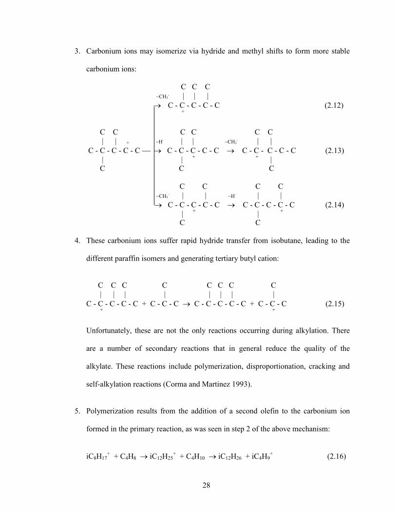
3. Carbonium� ions�may� isomerize�via� ydride�and�met yl� s ifts� to� form�more�stable���
carbonium�ions:�
�������������������������������������������������������C���C����C� ������������������������������������������~CH3
!�������|�����|������|� → C�!�C�!�C�!�C�!�C������������������������������������������������������(2.12)�
���������������������+�
� �������������C����C��������������������������������C���C������������������������������C����C� ��������������|������|�����+�����������������~H!���������|�����|����������������~CH3
!����������|������|� �C�!�C�!�C�!�C�!�C���→���C�!�C�!�C�!�C�!�C����→����C�!�C�!��C�!�C�!�C� ���������(2.13)�
��������������|����������������������������������������|�����+�������������������������������+��������|� �������������C��������������������������������������C�� � � � ����C� � ������������������������������������������������������C���������C� � ���������C���������C� ������������������������������������������~CH3
!��������|�����������|� �������~H!�����������|�����������|� � � � �����→���C�!�C�!�C�!�C�!�C����→����C�!�C�!�C�!�C�!�C� ���������(2.14)�
���������������������|�����+� � ����������|�����������+� ������������������������������C� � � ���������C� �
4. T ese� carbonium� ions� suffer� rapid� ydride� transfer� from� isobutane,� leading� to� t e�
different�paraffin�isomers�and�generating�tertiary�butyl�cation:�
� ������������C����C���C������������������C�� ��������C���C���C� � �����C� ������� �|������|�����|� ����������|�� ���������|�����|�����|� � ������|�
C�!�C�!�C�!�C�!�C��+��C�!�C�!�C��→��C�!�C�!�C�!�C�!�C��+��C�!�C�!�C��������������������(2.15)� �+� � � � � � � �� �����+�
� Unfortunately,� t ese� are� not� t e� only� reactions� occurring� during� alkylation.� T ere�
are� a� number� of� secondary� reactions� t at� in� general� reduce� t e� quality� of� t e�
alkylate.� T ese� reactions� include� polymerization,� disproportionation,� cracking� and�
self!alkylation�reactions�(Corma�and�Martinez�1993).�
� 5. Polymerization� results� from� t e� addition� of� a� second� olefin� to� t e� carbonium� ion�
formed�in�t e�primary�reaction,�as�was�seen�in�step�2�of�t e�above�mec anism:�
� iC8H17
+��+�C4H8��→�iC12H25 +��+�C4H10��→�iC12H26��+�iC4H9
+� � ����������(2.16)�
28�

�
T e�iC12H25 +�can�continue�to�react�wit �an�olefin�to�form�a�larger�isoalkyl�cation:�
� iC12H25
+��+�C4H8��→�iC16H33��+�iC4H10��→�iC16H34��+�iC4H9+� � ����������(2.17)�
� 6. Disproportionation�causes�t e�disappearance�of�two�molecules�of�alkylate�to�give�a�
lower�and�a� ig er�molecular�weig t�isoparaffin�t an�t e�initial�one:�
� 2iC8H18��→�iC7H16��+�C9H20� � � � � � ����������(2.18)�
� 7.��Larger�isoalkyl�cations�can�crack,�leading�to�smaller�isoalkyl�cations�and�olefins:�
�
→ �iC5H11 +��+�iC7H14�� � � � ����������(2.19)�
������������������������������������������������ ��������������������iC12H25
+��������� ������������������������������������������������������� �����������������������������������������→����iC6H13
+��+�iC6H12� � � � ����������(2.20)� � � �������iC6H13
+��→�iC5H11 +��+�iC5H10��+�iC6H12� � � � � ����������(2.21)�
���������������������� �������������������������������
8. Self!alkylation�accounts� for� t e�formation�of� trimet yl!pentanes�w en� isobutane� is�
alkylated�wit �olefins�ot er�t an�butanes.�At�t e�same�time,�saturated�paraffin�of�t e�
same�carbon�number�as�t e�olefin�is�obtained.�T e�reaction�sc eme�for�pentene,�for�
example�is�:�
��������������������+� � � � � � ������+� C�!�C�!�C�!�C��+�C�!�C�!�C�����C�!�C�!�C�!�C��+��C�!�C�!�C�� � ����������(2.22)� � �������|����������� ���|� � �������|� � ����|�� � ������C� � ��C� � ������C� � ���C� � � �+� C�!�C�!�C�����C�!�C�=�C��+�H+�� � � � � � ����������(2.23)� � �|� �����������|� ������C� ����������C�
� �
29�

�
� � � � ��������C� � ��+� � � ���������|� ���������+� �C�!�C�!�C�+�C�!�C�=�C��→��C�!�C�!�C�!�C�!�C� � ������������������ ����������(2.24)������� � ��|��������������������|�� ���������|� ���������|�� � �C� ����������C� ��������C���������C�� � T e�above�reactions�are�believed�to�be�fundamental�to�t e�alkylation�process�and�are�
used� to� explain� t e� formation� of� bot � primary� and� secondary� products.� Alt oug �
isobutane� and� butenes� were� used� as� examples,� t ese� reactions� also� applied� to� ot er�
isoparaffins�and�olefins.��
2.2.4 eaction Mechanism for Alkylation of Isobutane with Propylene
Langley�and�Pike� (1972)� studied� t e� sulfuric�acid�alkylation�of� isobutane�wit �
propylene� and� proposed� seventeen!reaction� mec anism� model� (Table� 2.2)� based� on�
Sc mering�carbonium�ion�mec anism�wit �modification� introduced� to�account�for� iC9�
and� iC10� formation.� Experimental� measurements� were� made� in� an� ideally� mixed,�
continuous�flow�stirred�tank�reactor�at�t e�temperature�range�18!57�oC.�T e�model�was�
found� to� be� valid� in� t e� range� of� 27!57� oC� using� 95%� sulfuric� acid� catalyst.� Lower�
concentration�of�sulfuric�acid�(around�90%)�resulted�in�increased�rates�of�formation�of�
iC9�and�iC10�and�decreased�rates�of�alkylate�formation.��
2.2.5 eaction Mechanism for Alkylation of Isobutane with Butylene and
Pentylene
Vic ailak�(1995)�extended�t e�mec anism�given�by�Langley�and�Pike�(1972)�to�
a�nineteen!reaction�mec anism�model�for�isobutane�wit �butylene�alkylation�and�twenty�
one!reaction� mec anism� model� for� isobutane� wit � pentylene� alkylation.� T e� reaction�
mec anism�model�for�alkylation�of�isobutane�wit �butylene�is�s own�in�Table�2.3.�T e�
reaction� rate� constants� (frequency� factor� and� activation� energy)� for� eac � reaction� of�
30�
�
t ese� mec anisms� t at� were� taken� to� be� identical� to� t e� reactions� in� t e� propylene�
mec anism.� A� list� of� t ese� rate� constants,� k� values,� are� given� in� Appendix� C.8.� T e�
results�from�t is�reaction�model�s owed�a�fair�agreement�(90%)�wit �t e�publis ed�data�
(Albrig t,� 1992,� Sric anac aikul,� 1996).� T e� reaction� mec anism� and� rate� constants�
s own� in� Table� 2.3� to� describe� t e� alkylation� reaction� were� used� for� t e� STRATCO�
reactors�in�t e�Motiva�plant�model.�
31�

� Table�2.2.�Reaction�Mec anism�and�Material�Balances�for�Sulfuric�Acid�Alkylation�of�Isobutane�wit � Propylene�(Langley,�1969)�
�
32�
� Initiation�reactions� � � � � (a)�Material�balance�on�reactants�and�� � � � � � � � ������Associated�consumption�rates.� �
= k1 + − + − + − 3C + HX →C 3 X � � � � − r = k [C X ][ C ] + k [ C X ][ C ] + �
C4 2 3 4 3 5 4
+ k + + +− − − −2C X + C →C + C X � � � � � k [ C X ][ C ] + k [ C X ][ C ] + �3 4 3 4 4 6 4 5 7 4
� � � � � � � � k [ C + X − ][ C ] + k [ C
+ X − ][ C ] + �
6 8 4 7 9 4
Primary�reactions� � � � � �� k [ C + X − ][ C ] �
8 10 4
+ = k + = + =− − −11 C4 X + C → C
7 X � � � − r = k [C ][HX ] + k [ C X ][C3] + �
3 C3= 1 3 11 4
− − −+ k + + = 5 C X + C → C + C X � � � ���� k [ C X ][C ] �7 4 7 4 15 7 3
Self-alkylation reactions
� � � � � � (b)�Product�formation�equations.�
+ k = +9 C X − → C + HX �� � �� r = k [C X − ][ C ] �
4 4 C3 2 3 4
+ = k + +− − −10 C X + C → C X � � � r = k [ C X ][ C �4 4 8 C5 3 5 4
+ k + +− − −6 C X + C → C + C X � � � r = k [ C X ][ C ] �8 4 8 4 C6 4 6 4
� � � � � � r = k [ C + X − ][ C ] �
C7 5 7 4
Destructive�alkylation�reactions� � � � r = k [ C + X − ][ C ] �
C8 6 8 4
+ k = +12 C X − → C + HX � � � r = k [ C X − ][ C ] �
7 7 C9 7 9 4
= + k = + +− − −13 C + C X → C + C X � � r = k [ C X ][ C ] �7 4 5 6 C10 8 10 4
= k +14 C5 + HX → C
5 X − �� � � (c)�Olefinic�intermediate�rate�equations.�
k + + = +− − − −3 C + X + C → C + C X � � r = 0 = k [ C X ] − k [ C ][ C X ] �5 4 5 4 C 4 = 9 4 10 4 4
− − − −+ k + = + +4 C6 X + C
4 → C + C4 X � � � r
5 = = 0 = k13[ C
7 ][ C4 X ] + k [ C10 X ] − �
6 C 17
+ = k + = = +− − −15 C X + C → C X ��������� � ������������������� k [ C ][HX ] − k [ C ][ C X ] �7 3 10 14 5 16 5 4
+ k + + = +− − − −8 C X + C → C + C X � � r = 0 = k [ C X ] − k [ C ][ C X ] �10 4 10 4 C7 = 12 7 13 7 4
− k 16 −= + +
C + C X → C X � � � (d)�Carbonium�ion�rate�equations.�5 4 9
+ k + = +− − −7 C X + C → C + C X � � � r = 0 = k [C ][HX ] − k [C X ][ C ] �9 4 9 4 C3+ X − 1 3 2 3 4
− − − −+ k = + + = +17 C X → C + C X � � � r = 0 = r − k [ C X ] − k [ C ][ C X ] − �10 5 5 C 4 + X − C 4 9 4 10 4 4
+ = = + � � � � � � � k [ C X − ][C ] − k [ C ][ C X − ] − �
11 4 3 13 7 4
� � � ������ � � � k [ C = ][ C
+ X − ] �
16 5 4
� � � � � � r = 0 = k [ C = ][HX ] + k [ C
+ X − ] − �
C5 + X − 14 5 17 10
� � � � � � � k [ C + X − ][ C ] �
3 5 4
+ − − � � � � � � r = 0 = k [ C
= ][ C X ] − k [ C
+ X ][ C ] �
C6 + X − 13 7 4 6 4
+ = + � � � � � � r = 0 = k [ C X − ][C ] − k [ C X − ][ C ] − �
C7 + X − 11 4 3 5 7 4
+ = + � � � � � � � k [ C X − ][C ] − k [ C X − ] �
15 7 3 12 7
= + + � � � � � � r = 0 = k [ C ][ C X − ] − k [ C X − ][ C ] �
C8 + X − 10 4 4 6 8 4
= + + � � � � � � r = 0 = k [ C ][ C X − ] − k [ C 9 X − [ C ] �
C9 + X − 16 5 4 7 4
+ = + � � � � � � r = 0 = k [ C X − ][C ] − k [ C X − ] − � �
C10 + X − 15 7 3 17 10
� � � � � � � � k [ C + X − ][ C ] �
8 10 4
�

� Table�2.3.�Reaction�Mec anism�and�Material�Balances�for�Sulfuric�Acid�Alkylation�of�Isobutane� wit �Butylene�(Vic ailak,�1995)�
�I�
�
P
S
�
�
D
�
�
�
�
�
33�
nitiation�reactions� � � � � (a)�Material�balance�on�reactants�and�� � � � � � � ������Associated�consumption�rates.� �
= k1 + − + + 4 + HX → 4 � � � − r = k [C X − ][ ]+ −C C X C k [ C X ][ C ]+ �
C4 2 4 4 3 5 4
− k 2 − − −+ + + +
C X + C →C + C X � � � ��������������� k [ C X ][ C ] + k [ C X ][ C ] + �4 4 4 4 4 6 4 5 7 4
� � � � � ��������������� k [ C + X − ][ C ] + k [ C
+ X − ][ C ] + �
6 8 4 7 9 4
− + − rimary�reactions� � � � � ��������������� k
8[ C
+ X ][ C ] + k
18[ C X ][ C ] �
10 4 11 4
+ = k + = + =− − −11 C X + C → C X � � � − r = k [C ][HX ] + k [ C X ][C ] + �4 4 8 C 4= 1 4 11 4 4
+ k + + =− − − + − = 6 C X + C → C + C X � � � ���������������� k [ C X ][C ] + k [ C X ][C ] �8 4 8 4 15 7 4 19 6 4
elf!alkylation�reactions� � � � (b)�Product�formation�equations.�
+ k = +9 C X − → C + HX �� � �� r = k [C X − ][ C ] �
4 4 C4 2 4 4
− = k + − −10 C + X + C → C X � � � r = k [ C
+ X ][ C ] �
4 4 8 C5 3 5 4
+ k + +− − −6 C X + C → C + C X � � � r = k [ C X ][ C ] �8 4 8 4 C6 4 6 4
� � � � � r = k [ C + X − ][ C ] �
C7 5 7 4
� � � � � r = k [ C + X − ][ C ] �
C8 6 8 4
estructive�alkylation�reactions� � � � r = k7[ C
9
+ X − ][ C ] �
C9 4
+ k = +12 C X − → C
8 + HX � � � � r10 = k
8[ C X − ][ C
4] �
8 C 10
= + k = +− − + −13 C + C X → C + C X �� � r = k [ C X ][ C ] �8 4 5 7 C11 18 11 4
= k +14 C5 + HX → C
5 X − �� � � (c)�Olefinic�intermediate�rate�equations�
+ − k + − + = +3 − − C X + C → C + C X � � � r = 0 = k [ C X ] − k [ C ][ C X ] � 5 4 5 4 C 4 = 9 4 10 4 4
+ − k + − = + +5 − − C X + C → C + C X � � � r = 0 = k [ C ][ C X ] + k [ C X ] − � 7 4 7 4 C5= 13 8 4 17 11
+ = k + = = +− − −15 C X + C → C X ��������� � ������������������� k [ C ][HX ] − k [ C ][ C X ] �7 4 11 14 5 16 5 4
+ k + + = +− − − −18 C X + C → C + C X �� � r = 0 = k [ C X ] − k [ C ][ C X ] �11 4 11 4 C8= 12 8 13 8 4
= + k +16 C + C X − → C X −
� � � (d)�Carbonium�ion�rate�equations.�5 4 9
+ k + = +− − −7 C X + C → C + C X � � � r = 0 = k [C ][HX ] − k [C X ][ C ] �9 4 9 4 C 4+ X − 1 4 2 4 4
+ − k = + − + − = + − C X → C + C X � � �������������� r = 0 = −r − k C X ] − k C ][ C X17 [ [ ] − �
11 5 6 C 4+ X − C 4 9 4 10 4 4
− − −+ = = + = + � � � � � � ������ k [ C X ][C ] − k [ C ][ C X ] − k [ C ][ C X ] �
11 4 4 13 8 4 16 5 4
� � � r = 0 = k [ C = ][HX ] − k [ C
+ X − ][ C ] �
C5+ X − 14 5 3 5 4
� � � � � � � � � � + + + − =
� � � r = 0 = k [ C X − ] − k C X
− ][ C ] − k C X ][ ] �[ [ C ���������������������
C 6+ X − 17 11 4 6 4 19 6 4
+ = ++ − k + − − − + − = 4 C
6 X + C → C6 + C X � � � r = 0 = k [ C X ][ C ] − k C X[ ][ C ] − k [
7][C
4 ] �4 4 C 7+ X − 13 4 8 5 7 4 15 C X
= + ++ − = k + − − − = 19 C X + C → C X � � � r = 0 = k [C ][ C X ] + k [ C X ][ C ] − �6 4 10 C8+ X − 11 4 4 10 4 4
+ − k + − + − + −8 C X + C → C + C X � � � � ������� k [ C X ][ C ] − k [ C X ] �10 4 10 4 6 8 4 12 8
= + + � � � � � r = 0 = k [ C ][ C X − ] − k [ C 9 X − [ C ] �
C9 + X − 16 5 4 7 4
+ − + − � � � � � r = 0 = k [ C X ][C
= ] − k C X ][[ C ] �
C10+ X − 19 6 4 8 10 4
− − −+ = + + � � � � � r = 0 = k [ C X ][C ] − k [ C X ][ C ] − k [ C X ] �
C11+ X − 15 7 4 18 11 4 17 11

�
2.2.6 Influence of Process Variables
T e� most� important� process� variables� are� reaction� temperature,� acid� strengt ,�
isobutane� concentration,� and� olefin� space� velocity.� C anges� in� t ese� variables� affect�
bot �product�quality�and�yield�(Gary�and�Handwerk,�1984).��
Reaction�Temperature�
� T e�reaction�temperature�in�sulfuric�acid�alkylation�is�usually�in�t e�range�of�32!
50� oF.� At� ig er� temperatures,� oxidation� reactions� become� important� and� acid�
consumption� increases� (Corma� and� Martinez,� 1993).� At� temperatures� above� 65� oF,�
polymerization� of� t e� olefins� becomes� significant� and� yields� are� decreased.� If� t e�
operation� takes� place� at� lower� temperatures,� t e� effectiveness� decreases� due� to� t e�
increase� in� t e�acid�viscosity�and� t e�decreased�solubility�of� ydrocarbons� in� t e�acid�
p ase�(Gary�and�Handwerk,�1984).��
Acid�Strengt �
Acid� strengt � as� varying� effects� on� alkylate� quality,� depending� on� t e�
effectiveness�of� t e� reactor�mixing�and� t e�water� content�of� t e� acid.� In� sulfuric� acid�
alkylation,� t e� best� quality� and� ig est� yields� are� obtained� wit � acid� strengt s� of� 93!
95%� by� weig t� of� acid,� 1!2%� of� water� and� t e� remainder� ydrocarbon� diluents.� T e�
water� content� in� t e� acid� lowers� its� catalytic� activity� by� about� 3!5� times� as� muc � as�
ydrocarbon� diluents,� t us,� an� 88%� acid� containing� 5%� water� is� muc � less� effective�
catalyst�t an�t e�same�strengt �acid�containing�2%�water.�At�concentrations� ig er�t an�
99%,�isobutane�reacts�wit �SO3,�and�below�85!88%�concentration,�t e�catalyst�becomes�
a� polymerization� rat er� t an� an� alkylation� catalyst.� Poor� mixing� in� a� reactor� requires�
ig er�acid�strengt �necessary�to�keep�acid�dilution�down.�Increasing�t e�acid�strengt �
34�
�
from� 89%� to� 93%� increases� t e� alkylate� quality� by� 1!2� octane� numbers� (Cupit� et.al.,�
1962).��
Isobutane�Concentration�
� Isobutane�concentration�in�t e�feed�to�t e�reactor�is�generally�expressed�in�terms�
of� isobutane/olefin� ratio.� T is� is� one� of� t e� most� important� process� variables� t at�
controls�acid�consumption,�yield�and�quality�of�t e�alkylate.�W en�t e�isobutane/olefin�
ratio� in� t e� feed� is� ig � (15:1),� t e� olefin� is� more� likely� to� react� wit � an� isobutane�
molecule� to� form� t e� desired� product� t an� to� undergo� butene!butene� polymerization.�
T us�undesired�reactions�are�minimized.� If� t is�ratio�is�kept� low�(<5:1),�production�of�
eavy� polymers� increases� due� to� polymerization� reactions,� and� t e� acid� consumption�
increases�(Corma�and�Martinez,�1993).�An�increase�in�t is�ratio�produces�a�decrease�in�
acid� consumption�w ile� increasing�bot � t e� yield� and� t e�quality�of� t e� alkylate.�T e�
external�isobutane�to�olefin�ratio�in�sulfuric�acid�plants�are�usually�in�t e�range�of�5:1�to�
15:1�(Gary�and�Handwerk,�1984).��
Olefin�Space�Velocity�
Olefin� space� velocity� is� defined� as� t e� volume� of� olefin� c arged� per� our�
divided�by�t e�volume�of�acid�in�t e�reactor.�
Volumetr c Flow Rate of Olef n � Olef n space veloc ty = �
Vol. Fract on of ac d n reactor *Volume of reactor
Lowering� t e� olefin� space� velocity� reduces� t e� amount� of� ig � boiling� ydrocarbons�
produced,� increase� t e� product� octane� and� lowers� acid� consumption� (Gary� and�
Handwerk,�1984).�Olefins�space�velocity�is�one�way�of�expressing�space!time,�anot er�
is�by�using�contact�time.�
35�

�
2.2.7 Feedstock
Olefins� and� isobutane� are� used� as� alkylation� feedstocks.� T e� c ief� sources� of�
olefins�are�catalytic�cracking�and�coking�operations.�Butenes�and�propenes�are�t e�most�
common�olefins�used�but�et ylene�and�pentenes�are�included�in�some�cases.�Olefins�can�
be�produced�by�de ydrogenation�of�paraffins�and�isobutane�is�cracked�commercially�to�
provide�alkylation�unit�feed.�
� Hydrocrackers�and�catalytic�crackers�produce�a�majority�of�t e�isobutane�used�in�
alkylation,� moreover� it� is� obtained� from� catalytic� reformers,� crude� distillation,� and�
natural� gas� processing.� In� some� cases,� normal� butane� is� isomerized� to� produce�
additional�isobutane�for�alkylation�unit�feed.�
2.2.8 Products
In� addition� to� t e� alkylate� stream,� t e� products� leaving� t e� alkylation� unit�
include� t e� propanes� and� normal� butane� t at� enter� wit � t e� saturated� and� unsaturated�
feed�streams�as�well�as�a�small�quantity�of�tar�produced�by�polymerization�reactions.�
� T e�product�streams�leaving�an�alkylation�unit�are:�
1. LPG�grade�propane�liquid�
2. Normal�butane��liquid�
3. C5+�Alkylate�
4. Spent�Acid�(wit �tar)�
Only�about�0.1�%�by�volume�of�olefin�feed�is�converted�into�tar.�T is�is�not�truly�a�tar�
but�a�t ick�dark�brown�oil�containing�complex�mixtures�of�conjugated�cyclopentadienes�
wit �side�c ains�(T omas,�1970).��
� �
36�

�
2.2.9 Catalysts
Concentrated� sulfuric� and� ydroflouric� acids� are� t e� only� catalysts� used�
commercially� today� for� t e� production� of� ig � octane� alkylate� gasoline� but� ot er�
catalysts� are� used� to� produce� et ylbenzene,� cumene� and� long� c ain� (C12� to� C16)�
alkylated�benzenes�(T omas,�1970).�
� T e� desirable� reactions� are� t e� formation� of� C8� carbonium� ions� and� t e�
subsequent�formation�of�alkylates.�T e�main�undesirable� reaction�is�polymerization�of�
olefins.� Only� strong� acids� can� catalyze� t e� alkylation� reaction� but� weaker� acids� can�
cause�polymerization�to�take�place.�T erefore�t e�acid�strengt s�must�be�kept�above�88�
%�by�weig t�H2SO4�or�HF�in�order� to�prevent�excessive�polymerization.�Sulfuric�acid�
containing�free�SO3�also�causes�undesired�side�reactions�and�concentrations�greater�t an�
99.3�%�H2SO4�are�not�generally�used�(T omas,�1970).�
� Isobutane� is� soluble� in� t e� acid� p ase� only� to� t e� extent� of� about� 0.1� %� by�
weig t�in�sulfuric�acid�and�about�3�%�in� ydroflouric�acid.�Olefins�are�more�soluble�in�
t e�acid�p ase�and�a�slig t�amount�of�polymerization�of� t e�olefins�is�desirable�as� t e�
polymerization�products�dissolve�in�t e�acid�and�increase�t e�solubility�of�isobutane�in�
t e�acid�p ase.�
� If�t e�concentration�of�t e�acid�becomes�less�t an�88�%,�some�of�t e�acid�must�
be� removed� and� replaced� wit � stronger� acid.� In� ydroflouric� acid� units,� t e� acid�
removed�is�redistilled�and�t e�polymerization�products�removed�as�t ick�dark�oil.�T e�
concentrated� HF� is� recycled� in� t e� unit� and� t e� net� consumption� is� about� 0.3� lb� per�
barrel�of�alkylate�produced�(Templeton�and�King,�1956).�
37�

�
� T e�sulfuric�acid�removed�must�be�regenerated�in�a�sulfuric�acid�plant�w ic �is�
generally�not�part�of�t e�alkylation�unit,�and�t e�acid�consumption�ranges�from�18�to�30�
lb�per�barrel�of�alkylate�produced.�Makeup�acid�is�usually�99.3�%�by�weig t�H2SO4.�
2.3 Summary�
� T is� c apter� reviewed� t e� literature� for� c emical� process� analysis� and� for� t e�
current� understanding� of� alkylation� process.� T e� next� c apter� describes� t e�
met odology� of� Advanced� Process� Analysis� System.� Subsequent� c apters� describe�
Motiva’s�Alkylation�process�and�t e�results�of�applying�t e�system�to�t is�process.��
38�

CHAPTE 3
METHODOLOGY
In t is c apter a detailed description is given for t e met odology used in t e
Advanced Process Analysis System. T e framework for t e Advanced Process Analysis
System was s own in Figure 1.1. T e main components of t is system are a
flows eeting program for process material and energy balances, an on-line optimization
program, a c emical reactor analysis program, a eat exc anger network design
program and a pollution assessment module. An overview of eac of t ese programs
was given in C apter 1.
C emical Reactor
Separation and Recycle
Heat Exc anger Network
Utilities
Figure 3.1: ‘Onion Skin’ Diagram for Organization of a C emical Process and
Hierarc y of Analysis.
T e Advanced Process Analysis System met odology to identify and eliminate
t e causes of energy inefficiency and pollutant generation is based on t e onion skin
diagram s own in Figure 3.1. Having an accurate description of t e process from online
optimization, an evaluation of t e best types of c emical reactors is done first to modify
and improve t e process. T en t e separation units are evaluated. T is is followed by
t e pinc analysis to determine t e best configuration for t e eat exc anger network
and determine t e utilities needed for t e process. Not s own in t e diagram is t e
39

pollution index evaluation, w ic is used to identify and minimize emissions. T e
following gives a detailed description of t e components of t e Advanced Process
Analysis System and ow t ey are used toget er to control and modify t e process to
maximize profit and minimize wastes and emissions.
3.1 Flowsheeting Program
T e first step towards implementing t e Advanced Process Analysis System is
t e development of t e process model, w ic is also known as flows eeting. T e
process model is a set of constraint equations, w ic represent a mat ematical model of
material and energy balances, rate equations and equilibrium relation for t e process.
Formulation of t e process model can be divided into two important steps.
Formulation of Constraints for Process Units: A process model can be
formulated eit er empirically or mec anistically. A mec anistic model makes use of
constraint equations depicting conservation laws (mass and energy balances),
equilibrium relations and empirical formulas. Advanced Process Analysis System uses
mec anistic models for analysis.
Mat ematically, constraints fall into two types: equality constraints and
inequality constraints. Equality constraints are material and energy balances or any
ot er exact relations ip in a process. Inequality constraints include demand for product,
availability of raw materials and capacities of process units.
Classification of Variables and Determination of Parameters: After t e
constraints are formulated, t e variables in t e process are divided into two groups:
measured and unmeasured variables. Measured variables are t e variables w ic are
directly measured from t e distributed control systems (DCS) and t e plant control
40

laboratory. T e remaining variables are t e unmeasured variables. For redundancy,
t ere must be more measured variables t an t e degree of freedom of t e equality
constraints.
Parameters in t e model can also be divided into two types: constant and time
varying parameters. Constant parameters do not c ange wit time and include reaction
activation energy, eat exc anger areas. Time-varying parameters include fouling
factors in eat exc angers and catalyst deactivation parameters. T ey c ange slowly
wit time and are related to t e degradation of performance of equipment.
Flowsim: T e program used for flows eeting in t e Advanced Process
Analysis System is called ‘Flowsim’. Flowsim provides a grap ical user interface wit
interactive capabilities. An example of t is interface is s own in Figure 3.2 for a simple
refinery, and t e comparable diagram for t e alkylation process is given in t e next
c apter, Figure 4.5. Process units are represented as rectangular s apes w ereas t e
process streams are represented as lines wit arrows between t ese units. Process units
and streams can be drawn by clicking t e corresponding icons on t e Flowsim window.
Eac process unit and stream in t e flows eet must ave a name and a description.
Process information is divided into t e following six categories; equality constraints,
inequality constraints, unmeasured variables, measured variables, parameters and
constants.
T e information in t e first five categories is furt er classified by associating it
wit eit er a unit or a stream in t e flows eet. For example, for a unit t at is a eat
exc anger, t e relevant information includes t e mass balance and eat transfer
41

equations, limitations on t e flowrates and temperatures if any, t e eat transfer
coefficient parameter and all t e intermediate variables defined for t at exc anger.
Figure 3.2 Example of Flowsim Screen for a Simple Refinery
For a stream, t e information includes its temperature, pressure, total flowrate,
molar flowrates of individual components etc. Information not linked to any one unit or
stream is called t e ‘Global Data’. For example, t e overall daily profit of t e process is
a global unmeasured variable because it is not related to any particular process unit or
stream.
42

T e sixt category of constants can be grouped into different sets based on t eir
p ysical significance. For example, constants related to eat exc angers can be placed
in one group and t ose related to reactors into anot er group.
Flowsim also as a sevent category of information called as t e ‘ent alpy
coefficients’. T is stores t e list of all t e c emical components in t e process and t eir
ent alpy coefficients for multiple temperature ranges. All of t is process information is
entered wit t e elp of t e interactive, user-customized grap ic screens of Flowsim.
T is concludes t e description of t e flows eeting part of t e Advanced Process
Analysis System. Appendix J is t e user’s manual, w ic gives a step-by-step
description of creating process models.
3.2 Online Optimization Program
Once t e process model as been developed using Flowsim, t e next step is to
conduct on-line optimization. On-line optimization is t e use of an automated system
w ic adjusts t e operation of a plant based on product sc eduling and production
control to maximize profit and minimize emissions by providing setpoints to t e
distributed control system. As s own in Figure 1.5, it includes t ree important steps:
combined gross error detection and data reconciliation, simultaneous data reconciliation
and parameter estimation and plant economic optimization. In combined gross error
detection and data reconciliation, a set of accurate plant measurements is generated
from data extracted from t e plant’s Distributed Control System (DCS). T is set of data
is used for estimating t e parameters in plant models. Parameter estimation is necessary
to ave t e plant model matc t e current performance of t e plant. T en economic
optimization is conducted to optimize t e economic model using t is current plant
43
model as constraints. T is generates set points for t e distributed control system to
move t e plant to optimal operating conditions.
Eac of t e above t ree-optimization problems in on-line optimization as a
similar mat ematical statement as following:
Optimi e: Objective function
Subject to: Constraints from plant model.
w ere t e objective function is a joint distribution function for data reconciliation, least
squares for parameter estimation and a profit function (economic model) for plant
economic optimization. T e constraint equations describe t e relations ip among
variables and parameters in t e process, and t ey are material and energy balances,
c emical reaction rates, t ermodynamic equilibrium relations, and ot ers.
To perform data reconciliation, t ere as to be redundancy in t e measurements,
i.e. t ere s ould be more measurements t an t e degrees of freedom in t e process
model. For redundancy, t e number of measurements to determine t e minimum
number of measured variables is given by t e degree of freedom, w ic is calculated
using t e following equation (Felder and Rousseau, 1986).
Degree of freedom = Total number of variables – Total number of equality
constraints + Number of independent chemical reactions.
Also, t e unmeasured variables ave to be determined by t e measured
variables, called observability. If an unmeasured variable can not be determined by a
measured variable, it is unobservable. T is is called t e ‘observability and redundancy
criterion’, w ic needs to be satisfied (C en, 1998).
Combined Gross Error Detection and Data econciliation: Process data
from distributed control system is subject to two types of errors, random errors and
44

gross errors. Gross errors must be detected and rectified before t e data is used to
estimate plant parameters. Combined gross error detection and data reconciliation
algorit ms can be used to detect and rectify gross errors in measurements for on-line
optimization. T ese algorit ms are: measurement test met od using normal distribution,
Tjoa-Biegler’s met od using contaminated Gaussian distribution, and robust statistical
met od using robust functions. T e t eoretical performance of t ese algorit ms as
been evaluated by C en, 1998.
Based on C en’s study, Tjao-Biegler’s met od or robust met od is used to
perform combined gross error detection and data reconciliation. It detects and rectifies
gross errors in plant data sampled from distributed control system. T is step generates a
set of measurements containing only random errors for parameter estimation. T en, t is
set of measurements is used for simultaneous parameter estimation and data
reconciliation using t e least-squares met od.
Simultaneous Data econciliation and Parameter Estimation: T e general
met odology for t is step is similar to t e met odology of combined gross error
detection and data reconciliation. T e difference is t at parameters in plant model are
considered as variables along wit process variables in simultaneous data reconciliation
and parameter estimation rat er t an being constants as in data reconciliation. Bot
process variables and parameters are simultaneously estimated. Based on C en’s study,
t e least squares algorit m is used to carry out combined gross error detection and data
reconciliation. T e data set produced by parameter estimation is free of any gross
errors, and t e updated values of parameters represent t e current state of t e process.
T ese parameter values are used in economic optimization.
45

Plant Economic Optimization: T e objective of plant economic optimization is
to generate a set of optimal operating setpoints for t e distributed control system. T is
set of optimal setpoints will maximize t e plant profit, satisfy t e current constraints in
plant model, meet t e requirements for t e demand of t e product and availability of
raw materials, and meet t e restriction on pollutant emission. Optimization can be
ac ieved by maximizing t e economic model (objective function) subject to t e process
constraints. T e objective function can be different depending on t e goals of
optimization. T e objectives can be to maximize plant profit, minimize energy use,
minimize undesired by-products, minimize waste/pollutant emission or a combination
of t ese objectives. T e result of economic optimization is a set of optimal values for all
t e measured and unmeasured variables in t e process. T ese are t en sent to t e
distributed control system (DCS) to provide setpoints for t e controllers.
On-line optimization program of Advanced Process Analysis System retrieves
t e process model and t e flows eet diagram from Flowsim. Additional information
needed to run online optimization includes plant data and standard deviation for
measured variables; initial estimates, bounds and scaling factors for bot measured and
unmeasured variables; and economic objective function. T e program t en constructs
t ree optimization problems s own in Figure 1.5 and uses GAMS (General Algebraic
Modeling System) to solve t em sequentially. Results of t ese t ree problems can be
viewed using t e grap ical interface of Flowsim. T is is illustrated in t e user’s manual
in Appendix J.
46

3.3 Chemical eactor Analysis Program
Having optimized t e process operating conditions for t e most current state of
t e plant, t e next step in Advanced Process Analysis System is to evaluate
modifications to improve t e process and reduce emission and energy consumption.
First, c emical reactors in t e process are examined. T e reactors are t e key units of
c emical plants. T e performance of reactors significantly affects t e economic and
environmental aspects of plant operation. T e formulation of constraints in t ese types
of units is very important and complicated owing to t e various types of reactors and
complex reaction kinetics. Unlike a eat exc anger w ose constraints are similar
regardless of types of equipment, t ere is a great variation in deriving t e constraints for
reactors.
T e c emical reactor analysis program of Advanced Process Analysis System is
a compre ensive, interactive computer simulation t at can be used for modeling various
types of reactors suc as plug flow, CSTR and batc reactors. T is is s own in Figure
1.3. Reaction p ases included are omogeneous gas, omogeneous liquid, catalytic
liquid, gas-liquid etc. T e options for energy models include isot ermal, adiabatic and
non-adiabatic.
T e kinetic data needed for t e reactor system includes t e number of reactions
taking place in t e reactor and t e number of c emical species involved. For eac
reaction, stoic iometry and reaction rate expressions also need to be supplied. P ysical
properties for c emical species can be retrieved from Flowsim.
Feed stream for t e reactor is obtained from Flowsim and its temperature,
pressure and flowrate are retrieved using t e results from on-line optimization. Finally,
47

t e dimensions of t e reactor and eat transfer coefficients are supplied. All of t is data
is used to simulate reactor conditions and predict its performance. Reactant
concentration, conversion, temperature and pressure are calculated as functions of
reactor lengt or space-time. T e results can be viewed in bot tabular and grap ical
form. T e user’s manual in Appendix J gives a step-by-step description of t e program.
As operating process conditions c ange, t e performance of reactors can vary to
a significant extent, also. T e reactor design program a wide range of different types of
reactors, w ic can be examined and compared to decide t e best reactor configuration
for economic benefits and waste reduction.
3.4 Heat Exchanger Network Program
T e optimization of c emical reactors is followed by eat exc anger network
optimization as s own in t e onion skin diagram in Figure 3.1. Most c emical processes
require eating and cooling of certain process streams before t ey enter anot er process
unit or are released into environment. T is eating or cooling requirement can be
satisfied by matc ing t ese streams wit one anot er and by supplying external source
of eating or cooling. T ese external sources are called as utilities, and t ey add to t e
operating cost of t e plant. T e Heat Exc anger Network program aims at minimizing
t e use of t ese external utilities by increasing energy recovery wit in t e process. It
also synt esizes a eat exc anger network t at is feasible and as a low investment
cost.
T ere are several ways of carrying out t e above optimization. Two of t e most
important ones are pinc analysis and mat ematical programming met ods. Pinc
analysis is based on t ermodynamic principles w ereas t e mat ematical met ods are
48

based on mass and energy balance constraints. T e Heat Exc anger Network Program
(abbreviated as THEN) is based on t e met od of pinc analysis.
T e first step in t e implementation of THEN is t e identification of all t e
process streams, w ic are important for energy integration. T ese streams usually
include streams entering or leaving eat exc angers, eaters and coolers. T e
flows eeting diagram of Flowsim is used in t e selection of t ese streams.
T e next step in t is optimization task involves retrieval of necessary
information related to t ese streams. Data necessary to perform eat exc anger network
optimization includes temperature, flowrate, film eat transfer coefficient and ent alpy
data. Ent alpy data can be in t e form of constant eat capacities for streams wit small
temperature variations. For streams wit large variations, it can be entered as
temperature-dependent ent alpy coefficients. Film eat transfer coefficients are needed
only to calculate t e areas of eat exc angers in t e new network proposed by THEN.
Temperature and flowrates of various process streams are automatically
retrieved from t e results of online optimization. T e setpoints obtained after t e plant
economic optimization are used as t e source data. P ysical properties suc as t e eat
capacities, ent alpy coefficients and film eat transfer coefficients are retrieved from
Flowsim.
T e t ird step in eat exc anger network optimization is t e classification of
streams into ot streams and cold streams. A ot stream is a stream t at needs to be
cooled to a lower temperature w ereas a cold stream is a stream t at needs to be eated
to a ig er temperature. Usually, streams entering a cooler or t e ot side of a eat
exc anger are ot streams w ereas streams entering t roug a eater or t e cold side of
49

a eat exc anger are cold streams. T e final step in t is problem requires t e
specification of minimum approac temperature. T is value is usually based on
experience.
Having completed all of t e above four steps, eat exc anger network
optimization is now performed using THEN. T ermodynamic principles are applied to
determine t e minimum amount of external supply of ot and cold utilities. Grand
Composite Curve is constructed for t e process, w ic s ows eat flows at various
temperature levels. A new network of eat exc angers, eaters and coolers is proposed,
w ic features t e minimum amount of external utilities. T is network drawn in a
grap ical format is called t e Network Grid Diagram. An example of a network grid
diagram is given in Figure 1.4. Detailed information about t e network can be viewed
using t e interactive features of t e user interface. T e user’s manual in Appendix J
provides a step-by-step description of t e program.
T e amount for minimum ot and cold utilities calculated by t e Heat
Exc anger Network Program is compared wit current amount of utilities being used in
t e process. If t e current amounts are greater t an t e minimum amounts, t e process
as potential for reduction in operating cost. T e network grid diagram synt esized by
THEN can be used to construct a eat exc anger network t at ac ieves t e target of
minimum utilities. Savings in operating costs are compared wit cost of modification of
t e existing network, and a decision is made about t e implementation of t e solution
proposed by THEN.
50

3.5 Pollution Assessment Program
T e final step in t e Advanced Process Analysis System is t e determination of
t e emissions from t e process and t e location w ere t ese pollutants are generated
wit in t e process. T e pollution assessment module of Advanced Process Analysis
System is called ‘T e Pollution Index Program’. It is based on t e Waste Reduction
Algorit m and t e Environmental Impact T eory as described in C apter 2. It defines a
quantity called as t e pollution index to provide a basis for measuring t e pollution
generated by t e process.
Environmental impact of a c emical process is caused by t e streams t at t e
process takes from and emits to t e environment. Only t ese input and output streams
are considered in performing pollution index analysis. Ot er streams, w ic are
completely internal to t e process, are excluded. In t e Pollution Index Program, t is
selection of input-output streams is automatically done based on t e plant information
entered in Flowsim.
T e next step in pollution index analysis is t e classification of output streams
into product and non-product streams. All streams w ic are eit er sold as product or
w ic are used up in a subsequent process in t e production facility are considered as
product streams. All ot er output streams, w ic are released into t e environment, are
considered as non-product streams. All non-product streams are considered as pollutant
streams w ereas all product streams are considered to ave zero environmental impact.
Pollution index of a stream is a function of its composition. T e composition
data for t e streams is retrieved from t e results of on-line optimization performed
earlier. T is can be eit er in terms of molar flowrates or fractions. Additional data
51
needed for pollution analysis is t e specific environmental impact potential values of
individual c emical species present in a stream. T ese values for various c emical
species are available in t e report on environmental life cycle assessment of products.
T e last piece of information required is t e relative weig ting factors for t e
process plant. According to t e Waste Reduction Algorit m, environmental impact of
c emical processes can be broadly classified into nine categories e.g. acidification,
p otoc emical oxidation etc. T e relative weig ting factors allow t e customization of
t e analysis to local conditions. T eir values depend on t e location of t e plant and its
surrounding conditions. For example, t e weig ting factor for p otoc emical oxidation
is ig er in areas w ic suffer from smog.
Having finis ed all of t e above prerequisite steps, t e pollution index program
is now called to perform t e analysis. Mass balance constraints are solved for t e
process streams involved, and equations of t e Environmental Impact T eory are used
to calculate t e pollution index values. Six types of pollution indices are reported for t e
process. T ree of t ese are based on internal environmental efficiency w ereas t e ot er
t ree are based on external environmental efficiency. Hig er t e values of t ese indices,
ig er is t e environmental impact of t e process.
T e pollution index program also calculates pollution indices for eac of t e
individual process streams. T ese values elp in identification of t e streams w ic
contribute more to t e overall pollution impact of t e process. Suitable process
modifications can be done to reduce t e pollutant content of t ese streams.
Every run of on-line optimization for t e process can be followed by pollution
index calculations. T e new pollution index values are compared wit t e older values.
52

T e comparison s ows ow t e c ange in process conditions affects t e environmental
impact. T us, t e pollution index program can be used in continuous on-line monitoring
of t e process.
3.6 Summary
To summarize, t e Flowsim program is used first to develop t e process model.
T e On-Line Optimization program is used to control t e process to maximize profit
and minimize pollutants, and in doing t is it as to continually update t e process
model to matc t e current state of t e plant. T is provides an accurate description of
t e process for off-line process modification analysis. T e C emical Reactor Analysis
program is used to determine t e best type of c emical reactors for t e process and to
optimize t eir performance. T e Heat Exc anger Network Program t en optimizes t e
eat recovery in t e system and minimizes t e amount of external utilities. Finally, t e
Pollution Index Program is called to carry out pollution analysis to measure t e
environmental impact of t e process and to direct c anges to reduce waste generation.
Subsequent c apters describe applying t is met odology in analyzing Motiva refinery
alkylation process.
53
CHAPTER 4
MOTIVA ALKYLATION PROCESS Advanced Process Analysis System was applied to a commercial alkylation
process at Motiva Refinery Complex in Convent, Louisiana. This chapter describes the
Motiva alkylation process and the simulation of the process developed with APAS.
Also, the validation of the process simulation is given, demonstrating that the
simulation predicts the performance of the plant.
4.1 Process Description
Motiva Alkylation process is a 15,000 BPD STRATCO Effluent Refrigerated
Alkylation Plant. The heart of the process is the STRATCO reactor or contactor, which
contacts the reactants in a high velocity propeller stream and removes heat from the
exothermic reaction.
In the STRATCO Effluent Refrigerated Alkylation process, light olefins
(propylene, butylenes) are reacted with isobutane in the presence of sulfuric acid
catalyst to form hydrocarbon, mainly in the iC7 to iC8 range, called alkylate. The
alkylate product is a mixture of gasoline boiling range branched hydrocarbons which is
blended with the refinery gasoline pool to increase the gasoline octane.
Process flow diagrams representing Motiva alkylation process are shown in
Figures 4.1, 4.2 and 4.3. These were prepared from P&ID’s of the plant. The reaction
section of the process is shown in Figure 4.1. The refrigeration, depropanizer and
deisobutanizer sections are shown in Figure 4.2. The saturate deisobutanizer section of
the alkylation process is shown in Figure 4.3.
The process has four reactor pairs and four acid settlers as shown in Figure 4.1.
In the reaction section there are three feed streams, the olefin feed (HC01), the
54

isobutane feed (HC03) and the recycled olefin/isobutane mixture (HC32). The olefin
feed contains the light olefins that are reacted with isobutane in the alkylation unit's
STRATCO stirred reactors. The isobutane stream is in excess to fully react with all of
the olefins being charged to the unit. The process units are described in this section.
4.1.1 STRATCO Contactor
The two feed streams (HC01 and HC03) are cooled by exchanging heat with the
net Contactor effluent stream (5E-628, 5E-628, 5E-630) from the suction trap/flash
drum (5C-614) as shown in Figure 4.1. The two streams are then combined and fed to
the STRATCO Contactors (5C-623 to 5C-630). The recycled olefin/isobutane stream is
fed to the Contactors separately (HC34, HC38, HC41, HC45).
The STRATCO Contactor, in which the alkylation reaction occurs, is a horizontal
pressure vessel containing a mixing impeller, an inner circulation tube and a tube
bundle to remove the heat generated by the alkylation reaction as shown in Figure 4.4.
The feed is injected into the suction side of the impeller inside the circulation tube. The
impeller rapidly disperses the hydrocarbon feed with acid catalyst to form an emulsion.
The emulsion is circulated by the impeller at high rates within the Contactor. The
sulfuric acid present within the reaction zone serves as a catalyst to the alkylation
reaction. The acid absorbs a small amount of hydrocarbon from side reactions and feed
contaminants which reduces the sulfuric acid concentration.
55

1
5E-628
5E-629, 630
5E-633
5C-614 Acid Settler 5C-631
Fresh Acid
5C-623
Acid Settler 5C-632
Acid Settler 5C-633
Acid Settler 5C-634
5C-629 5C-627
5C-625
Olefins Feed
HC01
C401
HC03 HC04
HC02
HC06 HC11 HC07
HC14 HC16
HC19
AC02
AC18
AC23
AC40
AC09
AC05
AC07
AC12 AC15
AC20
AC23
AC26
AC31
AC34 AC37
AC42
Spent Acid
AC45
HC23 HC22
HC27 HC25
HC28
HC29
HC30
R1
R3 R7
R10
R12 R16
R19
R20
R29
C403
C402
C301
HC32
HC38 HC34
HC45 HC41
2
3
5
4
HC31 M-2
S-2
M-1
3’
M-24
S-5
M-7
M-3
S-19 HC33
HC40
S-23
S-11
S-27
M-17 M-13
S-7
M-15
M-4
M-11
HC08 HC14
HC26 HC24
AC29
STRATCO Reactor
STFD
Isobutane
R2 R6
R11 R15
Figure 4.1. Reactor Section of the Alkylation Process
56

Figure 4.2. Refrigeration, Depropanizer and Deisobutanizer Sections of the Alkylation process
5C-622
Compressor 5E-634-639 , 5E-655, 656
Compressor KO Drum
Depropanizer Charge Drum
5C-618 5C-658
Depropanizer Charge
Caustic Settler
5E-641-644
5E-640
5C-616
Economizer Drum
5E-610-653
5E-611
5C-603
Depropanizer
5E-613
5C-604
To FCCU, Fuel Gas
5E-657, 658
5E-612
i-butane to Storage
5C-660
Fresh Caustic
5C-608
Mixer
Wash Water
5E-616
5E-617-620
5E-626
5E-696
5E-627, 647
5E-695
n-butane
Alkylate
5C-606
Alkylate Deisobutanizer
5C-607
5E-621-624
Fuel Gas
Alkaline Water
C301
C302
C303
C306 C307
C308
C309
C311
C310
C310 C312
C312B
C313
C314
C313A
C315
C316 C318
C319
C322
C321 C320
C325 C325
C327
C329
C328
C331
C332 Propane
LPG
C403
C404
C405
C406
C407
C408
C409 C410
Wash Water
C411
C405 C406
C407
C408
C409
C411
C410
C412 C415
C414
C415
C418
C419
IC4 from storage
C417
1
2
3
3’
4
5
Refrigerant Accumulator
5C-615
C329A
5
To IC4 Flush Pump
C425
C427 C405A
Discharge
5K-601
C314A
Discharge Water
6
7
S-34
S-23
C312A
C315
C317
M-33
S-41
C404 M-34
S-42
57

SC406
Accumulator
5C-601
5E-602
5C-602 Saturate DeIsobutanizer
Saturate DIB Reflux
SC402
SC403
SC404
SC407 SC408
SC410
5E-605 - 608
6
Saturate Saturate Feed 5E-601 i-butane to
storage SC401
SC411 SC409 SC412
5E-609A
SC413
5E-603 7
n-butane to storage
SC405
Figure 4.3. Saturate Deisobutanizer Section of the Alkylation Process
58

In order to maintain the desired spent acid strength (89.0 wt% H2SO4) in the last two of
the eight Contactors, fresh acid (98.5 wt% H2SO4) is continuously charged to the first
two Contactors, and an equivalent amount of 89.0 wt% spent acid is withdrawn from
the acid settler.
Figure 4.4. STRATCO Effluent Refrigeration Reactor (Yongkeat, 1996)
The hydrocarbon and acid are separated in four settlers 5C-631 to 5C-634 and
the acid-free hydrocarbon phase (HC22, HC23, HC25, HC27) flows from the top of the
acid settler through a backpressure control valve. Part of it goes into the tube side of the
contactor tube bundle (R1). The backpressure control valve is set at a pressure (60.0
psig) to maintain the contents of the settler in the liquid phase. As the hydrocarbon
stream passes through the control valve, its pressure is reduced to about 5.0 psig,
flashing a portion of the stream's lighter components, thereby, cooling the stream to a
temperature of about 30 °F. When the two-phase stream passes through the tube bundle,
additional vapor is generated as a result of absorbing heat generated by the alkylation
reaction.
4.1.2 Refrigeration Section
As shown in Figure 4.1, the second portion (HC29) of the hydrocarbon effluent
from the settler goes to the isobutane chiller (5E-633) and is used to reduce the
temperature of the isobutane feed stream. It then combines with the Contactor effluent
59

stream leaving the tube bundle and flows into the suction trap side of the suction
trap/flash drum (5C-614), where the liquid and vapor portions of this stream are
separated. The suction trap/flash drum is a two-compartment vessel with a common
vapor space. The net Contactor effluent is accumulated on one side of a separation
baffle and is pumped to the effluent treating section. The cold refrigerant condensate is
accumulated on the other side of the baffle. This effluent recycle stream consists mostly
of isobutane and is returned to the Contactor by the effluent recycle pump. The vapor
portions of both of these streams combine and flow to the suction of the refrigeration
compressor (5K-601) shown in Figure 4.2.
The compressor driven by an electric motor, increases the pressure of the
refrigerant vapor to allow condensing by cooling water. The vapor is condensed in two
steps to provide a higher concentration of propane in the depropanizer feed.
Liquid generated by the first bank of condensers (e.g. 5E-634-639) is separated
from the propane-rich vapor in the refrigerant accumulator (5C-615), further cooled by
the refrigerant cooler, and then flashed across a control valve. Vapor and liquid are
separated in an economizer (5C-616). The economizer vapor returns to an intermediate
stage of the compressor (5K-601) to be recompressed, while the liquid is returned to the
suction trap/flash drum (5C-614).
The remaining vapor portion of the compressor discharge stream (C310) flows
from the separator to the "total condenser" (5E-641-644). Liquid from the total
condenser is accumulated in the Depropanizer Charge Drum (5C-618), and ultimately
fed to the Depropanizer (5C-603) for stripping of propane before being sent to the
Alkylate Deisobutanizer (5C-606).
60

4.1.3 Depropanizer (5C-603)
The depropanizer feed stream is pumped from the charge drum to the
depropanizer feed caustic wash (5C-658) to neutralize acidic components. The
neutralized stream then flows to the depropanizer feed/bottoms exchanger (5E-610-5E-
653) before entering the tower, as shown in Figure 4.2.
The overhead propane vapor from the depropanizer (C325) is totally condensed
by cooling water and collected in the depropanizer reflux accumulator drum (5C-604).
A part of the liquid is refluxed to the column's top tray (C329), and the rest is further
cooled and sent to the LPG section (C328). The depropanizer bottoms product (C317)
temperature is reduced in the feed/bottoms exchanger (5E610-653). The stream then
enters a water-cooled exchanger (5E-611) before it is split into three portions, one each
for the Alkylate Deisobutanizer, the Contactor ( 3 ) and storage.
4.1.4 Alkylate Deisobutanizer (5C-606)
The net effluent from the suction trap/flash drum (5C-614) is heated in the
feed/effluent exchangers (5E-628; 5E-629, 5E-630) as shown in Figure 4.1 and then
treated with caustic to remove any traces of acid (5C-660 and 5C-608 in Figure 4.2).
The treated net effluent is fed to the alkylate deisobutanizer (DIB) tower (5C-606) to
strip isobutane from alkylate as shown in Figure 4.2. Two steam-fired thermosiphon
reboilers (5E-695, 5E-696) supply the majority of the heat to the lower portion of the
column by vaporizing liquid side draws (C411) from the column as well as the DIB
bottoms liquid (C408). A portion of the depropanizer bottoms is fed to the column as
the reflux (C322).
Normal butane is removed as a vapor side-draw (C412). The vapor is condensed
and cooled by cooling water (5E-627, 5E-647). The normal butane product (C415) can
61

be used for vapor pressure blending or sold. The rate of the normal butane product will
vary depending on the desired deisobutanizer alkylate product Reid Vapor Pressure
(RVP).
The overhead isobutane vapor is condensed by cooling water and accumulated
in the isobutane accumulator pot (5C-607). Make-up isobutane (C417) from storage is
added to the pot and the combined stream (C418) is sent to the Contactors to react with
the olefins ( 3’ ).
The deisobutanizer bottoms (C405) is the alkylate product. It is cooled by the
deisobutanizer feed/effluent exchanger (5E-616) and also a heat exchanger with cooling
water (5E-617-5E-620). The cooled alkylate (C407) is removed as a product and sent to
storage.
4.1.5 Saturate Deisobutanizer (5C-601)
Another source for isobutane is the saturate deisobutanizer (SatDIB) column (Figure
4.3), which strips isobutane from saturate feed coming from reformer unit of the
refinery (SC401). The saturate feed, containing mainly C4’s, flows to the SatDIB
feed/bottoms exchanger (5E-601) before entering the tower, as shown in Figure 4.3.
The overhead isobutane vapor is condensed by cooling water and a fraction of it (stream
SC413) is accumulated in the isobutane accumulator pot (5C-607, Figure 4.2). The
saturate deisobutanizer bottoms (SC403) are mainly n-butane product. It is cooled by
the SatDIB feed/bottoms exchanger (5E-601) and also by a heat exchanger with cooling
water (5E-603). The cooled n-butane (SC405) is sent to storage.
4.2 Process Simulation
This section describes the models of the various process equipments in the
alkylation process. The process flow diagram, as developed with Flowsim, the
62

flowsheet simulation tool of Advanced Process Analysis System, is shown in Figure
4.5.
The equipment in the plant can be categorized according to their functions as follows:
Reaction Zone:
• STRATCO Contactor
• Acid settler
Separation Zone:
• Depropanizer
• Alkylate Deisobutanizer
• Saturate Deisobutanizer
• Suction Trap Flash Drum
• Economizer
• Compressor
Heat Transfer Zone:
• Heat Exchangers
• Condensers
• Reboilers
Miscellaneous:
• Mixers
• Splitters
• Reflux Accumulators
The models are developed for each of these units and are given in this chapter.
63

The alkylation process involves mixtures of a variety of components. The
components and compositions of streams vary widely from one section to the other. For
record keeping, all the hydrocarbon streams in the plant are composed of the following
components:
1. C3- Propane and lower
2. C4= Butenes
3. iC4 iso-butane
4. nC4 normal-butane
5. iC5 iso-pentane
6. nC5 normal-pentane
7. iC6 iso-hexane
8. iC7 iso-heptane
9. iC8 iso-octane
10. iC9+ iso-nonane and higher
All the sulfuric acid streams in the plant are composed of:
11. H2SO4 sulfuric acid
12. Water and impurities
The streams carrying the reaction products from the contactors to the acid settlers
contain all of the twelve components.
64

Figure 4.5. Process flow diagram, as developed with the Flowsheet Simulation tool of Advanced Process Analysis System
65

4.2.1 STRATCO Contactor (5C-623)
The sulfuric acid alkylation reaction mechanism for pure propylene and pure
butylene feeds were shown in Tables 2.2 and 2.3. These are based on the Schmering
carbonium ion mechanism with modification introduced to account for iC9 and iC10
formation. The material balance on reactants and the product formation equations are
shown in the same tables. The parameters that affect the performance of the contactor
are:
1. Operating Temperature
2. Acid Strength
3. Isobutane Concentration
4. Olefin Space Velocity R2
HC07
R3
HC34
AC09
AC07
Figure 4.6: Contactor 5C-623
The contactor was modeled as of a Continuously Stirred Tank Reactor (CSTR)
with heat exchange. The intense mixing provided by the propellers ensures that there is
no spatial variation in concentration, temperature, or reaction rate throughout the vessel.
The composition and temperature of the exit stream were the same as those inside the
reactor.
Referring to Figures 4.1 and 4.6, the material and energy balance equations for
the contactor 5C-623 are as follows:
Description
Inlet streams: HC07 (isobutane- olefin mixture), HC34 (effluent recycle-mainly
isobutane), and AC07 (sulfuric acid catalyst)

Outlet streams: AC09
Coolant streams: R2 (in), R3 (out)
Material Balance
Overall:
Mass flowrate in – Mass flowrate out = 0 (4.1)
F + F + F − F = 0 (4.2)HC 07 HC 34 AC 07 AC 09
FR2 − FR3 = 0 (4.3)
where, FX is the total mass flow rate (metric ton/min) of stream X.
Component:
Mass flowrate in – Mass flowrate out + Mass generation rate = 0 (4.4)
i i i i a iF + F − F + r V MW = 0 (4.5)HC 07 HC34 AC 09 5C 623
ifor the hydrocarbon components. Here, r is the reaction rate of component i, in terms
of moles of i produced per unit time, per unit volume of the acid catalyst (metric ton
moles/(m3⋅min)), and MW i is the molecular weight of component i. The quantity
V5 aC 623 , shown in the material balance equations, is the volume of acid in the contactor,
and is typically 60 % of the total contactor volume.
Considering the degradation of the catalyst, the material balance equation for the acid
component can be written as
i i aF − F − R = 0 (4.6)AC 07 AC 09 5C 623
where, RaC is the rate of degradation of the acid (metric ton/min). The acid 5 623
degradation rate can be related to the volumetric flowrate of butylenes into the contactor
as follows (Graves 1999),
67

a C 4=R C 623 = 0.121Q (4.7)5 HC 07
The total mass flow rates are calculated as the sum of the component flow rates.
∑ FXi − FX = 0 (4.8)
The subscripts to the process variables like mass flow rates, specific enthalpies and
stream temperatures indicate the stream names, and their superscripts indicate the
component. The subscripts to the process parameters indicate the process unit they
represent.
The material in the contactor is a two-phase mixture, consisting of a
hydrocarbon phase and an acid phase. Since the reaction model assumes that all the
reactions occur in the acid phase, the concentrations shown in the reaction model
equations are those in the acid phase.
The olefin feed to the process is composed of about 45% lv butylenes (1-BUT +
C2B + T2B) and about 3.5% lv propylene among other paraffins. Because of the low
presence of propylene and the non-participation of paraffins in the alkylation reaction,
the reaction mechanism of alkylation of isobutane with pure butylene (Table 2.3) was
adopted. The reaction rate terms in Equation 4.5 is evaluated using corresponding
equations from Table 2.3. Appendix A shows the procedure followed for calculating the
concentrations of the contactor components in the acid phase.
Alkylation of isobutane with olefins is an exothermic reaction. The reaction
mixture must be maintained in a particular temperature range (0-10 °C) in order to
obtain the desired yields. Higher operating temperatures result in oxidation and
polymerization reactions, decreasing the yields. Lower temperatures result in decreased
68
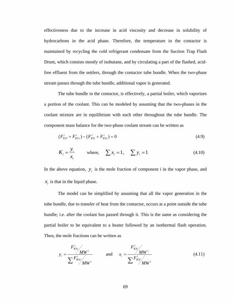
effectiveness due to the increase in acid viscosity and decrease in solubility of
hydrocarbons in the acid phase. Therefore, the temperature in the contactor is
maintained by recycling the cold refrigerant condensate from the Suction Trap Flash
Drum, which consists mostly of isobutane, and by circulating a part of the flashed, acid-
free effluent from the settlers, through the contactor tube bundle. When the two-phase
stream passes through the tube bundle, additional vapor is generated.
The tube bundle in the contactor, is effectively, a partial boiler, which vaporizes
a portion of the coolant. This can be modeled by assuming that the two-phases in the
coolant mixture are in equilibrium with each other throughout the tube bundle. The
component mass balance for the two-phase coolant stream can be written as
i i i i(F + F ) − (F + F ) = 0 (4.9)R2l R2v R3l R3v
yKi =i where, ∑ xi = 1, ∑ yi = 1 (4.10)
xi
In the above equation, yi is the mole fraction of component i in the vapor phase, and
xi is that in the liquid phase.
The model can be simplified by assuming that all the vapor generation in the
tube bundle, due to transfer of heat from the contactor, occurs at a point outside the tube
bundle; i.e. after the coolant has passed through it. This is the same as considering the
partial boiler to be equivalent to a heater followed by an isothermal flash operation.
Then, the mole fractions can be written as
i iFR3v FR3l MW i MW i
y = and xi = i (4.11)i FRi 3v FR3l
i ∑∑ MW MW i
69
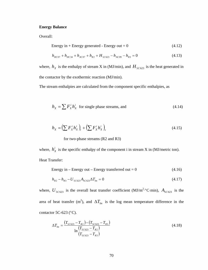
Energy Balance
Overall:
Energy in + Energy generated - Energy out = 0 (4.12)
hHC 07 + hHC34 + hAC 07 + hR2 + H 5C 623 − hAC 09 − hR3 = 0 (4.13)
where, h is the enthalpy of stream X in (MJ/min), and H is the heat generated inX 5C 623
the contactor by the exothermic reaction (MJ/min).
The stream enthalpies are calculated from the component specific enthalpies, as
hX =∑ FXi hX
i for single phase streams, and (4.14)
i i i ihX = (∑ FX hX )l + (∑ FX hX )v (4.15)
for two-phase streams (R2 and R3)
where, hXi is the specific enthalpy of the component i in stream X in (MJ/metric ton).
Heat Transfer:
Energy in – Energy out – Energy transferred out = 0 (4.16)
hR2 − hR3 −U 5C 623 A5C 623ΔTlm = 0 (4.17)
where, U 5C 623 is the overall heat transfer coefficient (MJ/m 2⋅°C⋅min), A5C 623 is the
area of heat transfer (m2), and ΔTlm is the log mean temperature difference in the
contactor 5C-623 (°C).
(T − T )− (T − T )5C 623 R2 5C 623 R3ΔTlm = (4.18)(T − T )5C 623 R2ln (T5C 623 − TR3 )
70
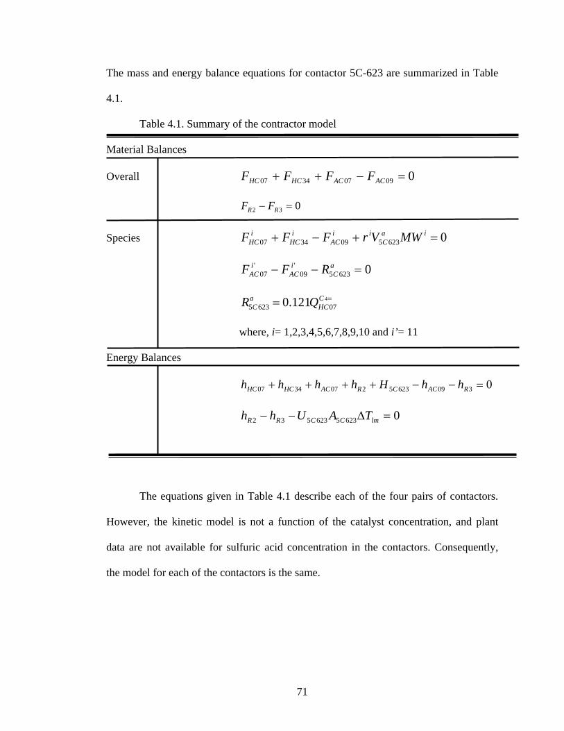
The mass and energy balance equations for contactor 5C-623 are summarized in Table
4.1.
Table 4.1. Summary of the contractor model
Material Balances
Overall FHC 07 + FHC 34 + FAC 07 − FAC 09 = 0
F − FR 2 R3 = 0
Species iFHC 07 i+ FHC34
i− FAC 09 i a i+ r V MW5C 623 = 0
i 'FAC 07 i '− FAC 09
a− R5C 623 = 0
a C 4=R = 0.121Q5C623 HC07
where, i= 1,2,3,4,5,6,7,8,9,10 and i’= 11
Energy Balances
h + h + h + h + H − h − h = 0HC07 HC34 AC 07 R2 5C 623 AC 09 R3
h − h −U A ΔT = 0R2 R3 5C 623 5C623 lm
The equations given in Table 4.1 describe each of the four pairs of contactors.
However, the kinetic model is not a function of the catalyst concentration, and plant
data are not available for sulfuric acid concentration in the contactors. Consequently,
the model for each of the contactors is the same.
71

4.2.2 Acid Settler (5C-631)
The acid settler separates the emulsion from the contactor into the acid and
hydrocarbon phases. One acid settler is provided to each pair of contactors. The inputs
to the settler are the effluents from the contactor pair and the outputs are the separated
acid and hydrocarbon streams.
The material and energy balance equations for the acid settler (5C-631) are as
shown in Table 4.2. The mass flow rate of each component coming in is equal to the
mass flow rate of each component leaving of the settler. Since there is no heat
transferred from or into the settler, the temperatures of the various input and output
streams can be assumed to be equal. We also assume that the separation of the two
phases in the settler is complete, so that there is no acid component in the output
hydrocarbon stream and vice-versa.
Table 4.2. Summary of the acid settler model
Material Balances
F i − F i = 0 i=1,2,3,4,5,7AC 09 HC 27
11 12F + F − F − F = 0AC 09 AC 09 AC 05 AC12
11 11F − s F = 0AC 05 C 631 AC 09
12 12F − s F = 0AC 05 C 631 AC 09
11 11x − x = 0AC 05 AC12
Energy Balances
T = T ; T = T ; T = TAC 09 HC 27 AC 09 AC12 AC 09 AC 05
72

4.2.3 Depropanizer (5C-603)
The Depropanizer was modeled using Smith-Brinkley Group method (Smith,
1963; Perry et al., 1984). This method can be applied to absorption, extraction
processes and distillation. The equation, which applies to the distillation process, is for
each component i,
N −M(1+ S )+ R(1− S )n,i nf = (4.19)N −M N −M M +1(1+ S )+ R(1− S ) + hS (1− S )n,i n n m
where R is the external-reflux ratio FC329/FC328 and f = (FiC317/Fi
C316), is the fraction of i
leaving in the bottoms product. The quantity S is the stripping factor (for each
component) and is defined for each group of stages in the column by Sn,i=KiV/L and
Sm,i=K'iV'/L'. K is the equilibrium ratio y/x for each component and V, L are the vapor
and liquid molar flow rates in the column. The Ki, V and L values are the effective
values for the top column section; K'i, V' and L' are the effective values for the section
below the feed stage. The quantity h depends on whether K or K' is used for the feed
stage. If the feed is mostly liquid, the feed stage is grouped with the lower stages and
K 'i L ⎛ 1− Sn ⎞hi = ⎜⎜ ⎟⎟ (4.20)KiL' ⎝1− Sm ⎠i
If the feed is mostly vapor,
L ⎛ 1− Sn ⎞hi = ⎜⎜ ⎟⎟ (4.21)L' 1− Sm ⎠⎝ i
The following four specifications for the column are necessary:
1. N, the total number of equilibrium stages
2. M, the number of stages below the feed stage
3. The reflux rate or the maximum vapor rate at some point in the column
73

4. The distillate rate D
Specification of D and L (or V), along with specifications of the feed stream
variables fixes the assumed phase rates in both sections of the column. Determination of
separation factors Sn and Sm then depends upon estimation of individual K values. If
ideal solutions are assumed, K values are functions of only temperature and column
specified pressure. Estimation of K values and, in turn, Sn and Sm values for each
component reduces to estimation of the effective temperature in each column section or
group of stages.
The effective temperature is assumed to be the arithmetic average for simplicity.
(T + T )N M +1Tn = (4.22)2
(T + T )M +1 1Tm = (4.23)2
The feed enters the column at the (M+1)th stage. The material and energy balance
equations for the depropanizer are shown in Table 4.3. The Saturate Deisobutanizer
column is modeled in a similar way.
74

Table 4.3. Summary of the depropanizer model
Material Balances
Overall F + F − F − F = 0C 316 C 329 C317 C 325
i i i iSpecies F + F − F − F = 0C 316 C 329 C317 C 325
where i=1,3,4,5
Smith- Brinkley Method Equations
K = f (P ,T )i C 603 n
K ' = f (P ,T )i C 603 m
K Fi C325S = n,i FC329
Ki 'V '
S = m,i 'L
N −M
f =(1+ S )+ R(1− S )n,i n,i
i N −M N −M M +(1+ S )+ R(1− S )+ h S (1− S 1 )n,i n,i i n,i m,i
F i C 317f = i iFC316
K 'i L ⎛ 1− Sn ⎞hi = ⎜⎜ ⎟⎟ K L' 1− Si ⎝ m ⎠i
where i=1,3,4,5,7
xi − xi = 0 , where i=1,3,4,5C 317 C 323
TC 317 − TC 323 = 0
75

4.2.4 Alkylate Deisobutanizer (5C-606)
The alkylate deisobutanizer column has two feed streams, two product streams,
two side streams and two reboilers, one of which is used as a side reboiler. One of the
feed streams is fed to the column, at the top tray, in place of the reflux. There was no
readily available short cut method to model such a distillation column as it is, therefore,
the column was divided into three reasonable sections (C-606A, C-606C and C-606D)
which can be modeled using Smith Brinkley Method and by employing equilibrium
stage assumption. General Smith-Brinkley Method is used for a classical distillation
column with recycle and reboiler streams, however the model of deisobutanizer requires
the derivation of the method for the rectifying and stripping sections separately.
Derivations can be found in (Smith, 1963) – Design of Equilibrium Stage Processes.
The equations for the alkylation deisobutanizer are given in Table 4.4.
76

Table 4.4. Summary of the deisobutanizer model
Material Balances
Overall
Species
F + F + F − F − F = 0C 404 C 432 C 322 C 414 C 430
F + F − F − F = 0C 430 C 427 C 431 C 425
F − F − F = 0C 426 C 428 C 405
F − F = 0C 427 C 431
F − F = 0C 425 C 430
i i i i iF + F + F − F − F = 0C 404 C 432 C 322 C 414 C 430
i i i iF + F − F − F = 0C 430 C 427 C 431 C 425
i i iF − F − F = 0C 426 C 428 C 405
where i=1,3,4,5
Smith- Brinkley Method Equations
Ki ,C 606 A = f (PC 606 A ,Tn,C 606 A )
'Ki,C606 A = f (PC 606 A ,Tm,C 606 A )
=Ki ,C 606C f (PC 606C ,TC 425 )
'Ki,C 606D = f (PC 606D ,Tm,C606D )
K ' V ' i ,C 606 A C 606 AS = m,i ,C 606 A 'LC 606 A
K Fi ,C 606 A C 414S = n,i ,C 606 A FC 322
K Fi,C 428 C 428=Sm,i ,C 606 D FC 426
77

Table 4.4. Summary of the deisobutanizer model (Cont’d)
Smith- Brinkley Method Equations
N −M S N −M(1− S )+ q (S − S ) +n,i,C 606 A i,C 606 A n,i,C 606 A n,i,C 606 A
F N −M Mq h S (1− S )i,C 606 A i,C 606 A n,i,C 606 A m,i,C 606 Af = i ,C 606 A N −M N −M M +1(1− S )+ h S (1− S )n,i,C 606 A i,C 606 A n,i ,C 606 A m,i ,C 606 A
F i C 430f = i,C 606 A i i i(F + F + F )C 404 C 322 C 432
F ⎛ 1− S ⎞C322 n,C606 Ah = ⎜ ⎟i,C 606 A ' ⎜ ⎟L 1− SC 606 A ⎝ m,C 606 A ⎠ i
' M −1DF K (S −1)+ F (S −1)M C 428 i ,C 606D m,i ,C 606D C 426 m,i ,C 606Dx = i ,C 606D 2F (S −1)C 426 m,i ,C 606D
where i=1,3,4,5,7
i i ixx K − xx = 0 , where i=1,3,4,5C 425 C 606C C 431
xi − xi = 0 , where i=1,3,4,5C 408 C 405
L' = F + q FC 606 A C 322 C 606 A C 404
V ' = FC 606 A C 432
T 431 − T = 0C C 425
78

x
4.2.5 Suction Trap/Flash Drum (5C-614)
The suction trap/flash drum (STFD) splits the hydrocarbon effluent from the
settlers based on volatility. It is a two-compartment vessel, with a common vapor space.
The net contactor effluent is accumulated on one side of the baffle and the cold
refrigerant condensate on the other. The vapors from the two compartments combine,
and flow out from the top.
The STFD is modeled as two C301 C302
separate units – suction trap and flash drum,
HC31 C311 with the vapor streams from the two units C401 HC32
combining in a mixer, as shown in Figure Suction Trap Flash Drum
4.7. The suction trap acts as the separating
Figure 4.7: STFD 5C-614vessel for the two-phase contactor from the
contactor tube bundles and from the isobutane chiller (5E-633). The liquid and vapor
streams leave the vessel as two separate streams. In the Flash drum, the cold condensate
from the economizer is flashed and separated. This unit is modeled as an equilibrium
stage with adiabatic flash. The material and energy balance equations for the two units
are as follows:
Suction Trap:
Overall material balance: (F + F ) − (F + F ) = 0 (4.24)HC 31l HC 31v C 401 C 301
F − F = 0 (4.25)HC 31l C 401
i i i iComponent material balance: (F + F )− (F + F )= 0 (4.26)HC31l HC31v C 401 C301
F i − F i = 0 (4.27)HC31l C 401
79
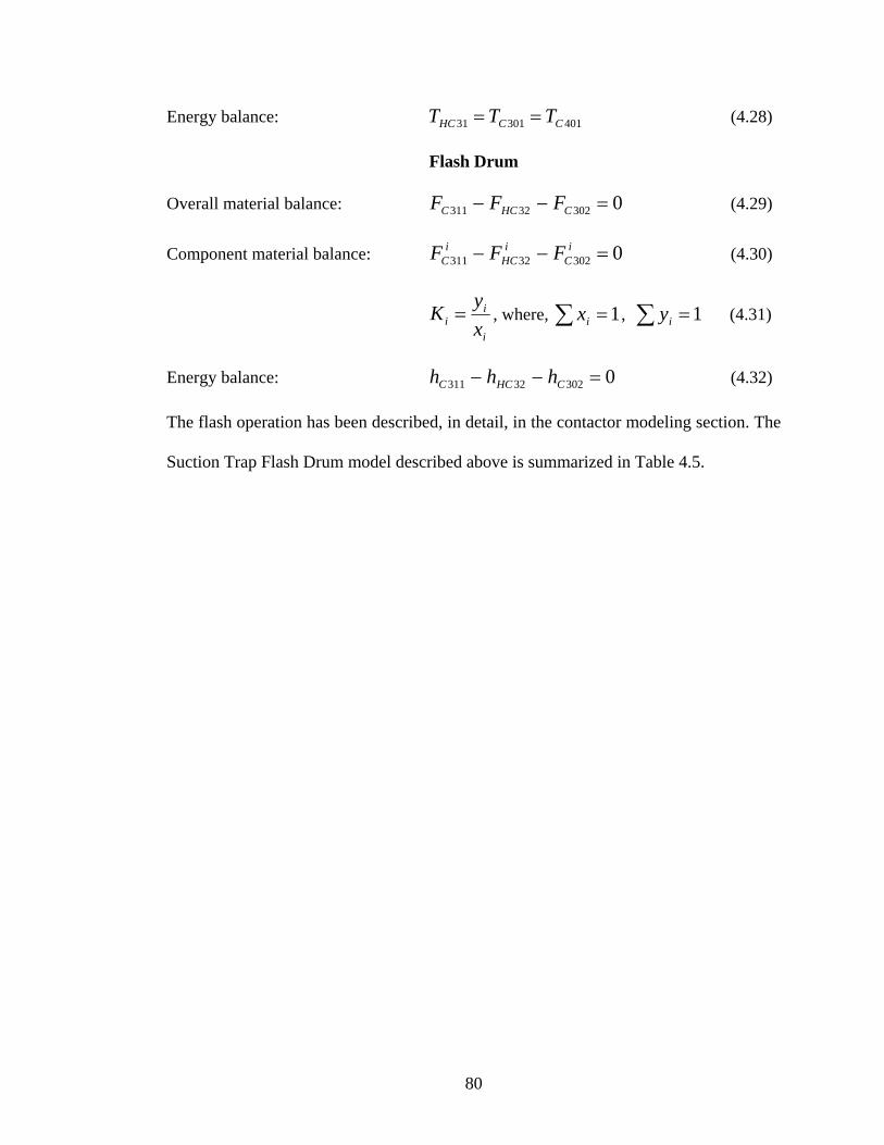
Energy balance: T = T = T (4.28)HC 31 C 301 C 401
Flash Drum
Overall material balance: F − F − F = 0 (4.29)C 311 HC 32 C 302
i i iComponent material balance: F − F − F = 0 (4.30)C311 HC32 C302
yKi = i , where, ∑ xi = 1, ∑ yi = 1 (4.31)xi
Energy balance: h − h − h = 0 (4.32)C 311 HC 32 C302
The flash operation has been described, in detail, in the contactor modeling section. The
Suction Trap Flash Drum model described above is summarized in Table 4.5.
80

Table 4.5. Summary of the suction trap/flash drum model
Material Balances
Overall
Species
(F + F ) − (F + F ) = 0HC 31l HC 31v C 401 C 301
F − F = 0HC 31l C 401
F − F − F = 0C 311 HC 32 C 302
i i i i(F + F )− (F + F )= 0HC31l HC31v C 401 C301
F i − F i = 0HC31l C 401
i i iF − F − F = 0 , where i=1,3,4,5,7C311 HC32 C302
yKi = i , where, ∑ xi = 1, ∑ yi = 1 xi
Energy Balances
T = T = THC 31 C 301 C 401
h − h − h = 0C 311 HC 32 C302
81

4.2.6 Economizer (5C-616)
The Economizer separates the vapor and liquid
phases generated when the liquid portion of the
propane-rich vapor, in the Depropanizer section, is
flashed. This unit is modeled the same way as the flash
C309
C311
C310
drum of STFD, i.e. assuming an adiabatic flash Figure 4.8. Economizer 5C-616
operation, where the two phases generated are in equilibrium with each other. The mass
and enthalpy balances are:
Overall material balance:
F − F − F = 0 (4.33)C309 C310 C 311
Component material balance:
i i iF − F − F = 0 (4.34)C309 C310 C311
yKi = i , where, ∑ xi = 1, ∑ yi = 1 (4.35)xi
In the above equation, Ki is the distribution coefficient or the K-factor, yi is the mole
fraction of component i in the vapor phase, and xi is that in the liquid phase.
Enthalpy balance:
h − h − h = 0 (4.36)C 309 C 310 C 311
where, hX is the enthalpy of stream X.
4.2.7 Compressor (5K-601)
The combined vapor stream from Suction Trap and the Flash Drum is rich in
propane, and is sent to the depropanizer section. The vapor is compressed in the
82

Refrigeration compressor (5K-601), to allow condensing by cooling water. The
compressor was assumed to operate under adiabatic conditions, and hence the
calculations were based on the following formulas (Perry et al., 1984):
Adiabatic head is expressed as
(k −1)⎡ ⎤k ⎛ p ⎞Had = RT1 ⎢
⎢⎜⎜
2 ⎟⎟
k − 1
⎥⎥ (4.37)
k − 1 ⎝ p1 ⎠⎢ ⎥⎦⎣
where Had = adiabatic head, ft; R = gas constant, (ft⋅lbf)/(lb⋅°R) = 1545/molecular
weight; T1 = inlet gas temperature, °R; p1 = absolute inlet pressure, lbf/in 2;
p2 = Absolute discharge pressure, lbf/in2, pk = ratio of specific heat capacities ( c cv ).
The work expended on the gas during compression is equal to the product of the
adiabatic head and the weight of the gas handled. Therefore, the adiabatic power is as
follows:
(k −1)⎡ ⎤WH k WRT ⎛ p ⎞ k
ad 1 ⎢ 2 ⎥hp = = ⎜⎜ ⎟⎟ − 1 (4.38)ad 550 k − 1 550 ⎢⎝ p1 ⎠ ⎥ ⎢ ⎥⎦⎣
(k −1)⎡ ⎤ −3 k ⎛ p ⎞
or hp = 4.36 ×10 Q1 p ⎢⎢⎜⎜
2 ⎟⎟
k − 1
⎥⎥ (4.39)ad k − 1 1
⎝ p1 ⎠⎢ ⎥⎦⎣
where hpad = power, hp; W = mass flow, lb/s; and Q1 = volume rate of gas flow,
ft3/min.
Adiabatic discharge temperature is:
83

(k −1) ⎛ p ⎞ k
T =T ⎜⎜ 2 ⎟⎟ (4.40)2 1 p⎝ 1 ⎠
C303
C310
C304
Figure 4.9: Compressor 5K-601
The constraint equations, for the compressor, are developed using the above formulas.
Overall material balance:
F + F − F = 0 (4.41)C 303 C 310 C304
Component material balance:
i i iF + F − F = 0 (4.42)C303 C310 C304
Enthalpy balance:
h + h + hp − h = 0 (4.43)C 303 C 310 ad C 304
(k −1) ⎛ p ⎞ k
T2 =T1 ⎜⎜ 2 ⎟⎟ (4.44)
p⎝ 1 ⎠
where hpad is the compressor as given in Equations (4.38, 4.39). The constraints of the
compressor are summarized in Table 4.6.
Table 4.6. Summary of the compressor model
84
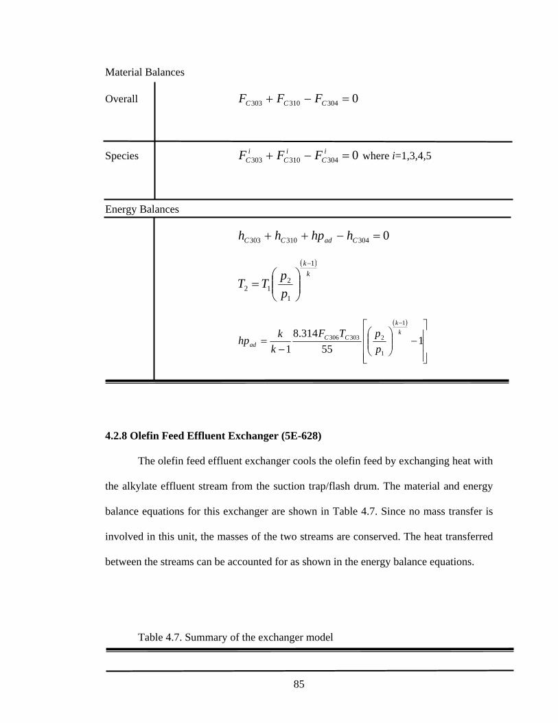
Material Balances
Overall F + F − F = 0C 303 C 310 C304
i i iSpecies F + F − F = 0 where i=1,3,4,5C303 C310 C304
Energy Balances
h + h + hp − h = 0C 303 C 310 ad C 304
(k −1) ⎛ p ⎞ k
T2 = T1 ⎜⎜ 2 ⎟⎟ p⎝ 1 ⎠
(k −1)⎡ ⎤ kk 8.314FC 306TC303 ⎢⎛ p2 ⎞ ⎥hp = ⎜⎜ ⎟⎟ −1ad k −1 55 ⎢⎝ p1 ⎠ ⎥
⎢ ⎥⎦⎣
4.2.8 Olefin Feed Effluent Exchanger (5E-628)
The olefin feed effluent exchanger cools the olefin feed by exchanging heat with
the alkylate effluent stream from the suction trap/flash drum. The material and energy
balance equations for this exchanger are shown in Table 4.7. Since no mass transfer is
involved in this unit, the masses of the two streams are conserved. The heat transferred
between the streams can be accounted for as shown in the energy balance equations.
Table 4.7. Summary of the exchanger model
85

Material Balances
F + F = 0Overall HC 01 HC02
F + F = 0C 401 C 402
xi + xi = 0Species HC01 HC02
xi + xi = 0C 401 C 402
where i= 1,2,3,4,5
Energy Balances
(h − h ) − (h − h ) = 0HC 02 HC01 C 401 C 402
(h − h ) −U A ΔT = 0HC 01 HC 02 5E 628 5E628 lm
(T − T )− (T − T )HC 02 C 401 HC 01 C 402ΔTlm = (T − T )HC 02 C 401ln (THC 01 − TC 402 )
86

4.3 Model Validation
The accuracy of the alkylation process model to predict the performance of the
plant has to be established. This model validation was performed by solving the data
validation problem using a set of plant data (steady state operation point #1) and then
comparing the results of the model with the plant data. For the 125 measured plant
variables, 88 were within the accuracy of the measurements. The remaining 37 variables
are shown in Table 4.8 for the plant data from the DCS, their reconciled value and the
standard measurement error ∈i (∈i = |yi -xi |/σi, where is σi the standard deviation of the
process variable). In consulting with the alkylation plant process engineers, it was
concluded that these 37 variables were within the range of possible process values. This
includes FC316, FC322, x5C417, xx5C412, xx7C414. The discrepancy in the variable
xx1C322 is a result of the model assumption that the propane purge from the drum 5C-
618 occurs infrequently. In summary, the model of the process accurately predicts its
performance and therefore can be used for on-line optimization.
Table 4.8. Plant vs. Model Data
Variable Name Plant Data (yi)
Reconciled Data from Data Validation
(xi)
Standard Measurement
Error (∈i)
FAC02 0.1125 0.1600 4.2235 FAC12 0.1259 0.1600 2.7085 FAC23 0.1253 0.1600 2.7653 FAC45 0.1040 0.1600 5.3846 FC308 2.1990 3.1032 4.1120 FC316 0.6581 1.8000 17.3515 FC322 0.4427 1.5619 25.2812 FC328 0.0942 0.0535 2.6399 FC403 3.8766 2.2834 4.1097 FC412 0.0324 0.0418 2.8968
FSC411 2.7287 1.3525 5.0436 FstmE612 0.1425 0.0889 3.7607
87

x1C417 0.0372 0.0255 3.1309 x2SC402 0.0136 0.0084 3.7929 x2SC408 0.0221 0.0002 9.9048 x3C325 0.0017 0.0000 10.0000
x3SC403 0.0103 0.0212 10.5665 x4C316 0.0580 0.0796 3.7155
x4SC408 0.0331 0.0088 7.3475 x5C316 0.0020 0.0060 19.8000 x5C417 0.0009 0.0295 286.2300 x5HC32 0.0096 0.0306 22.0134 x6SC402 0.0167 0.0666 29.8204 x6SC403 0.0250 0.0950 27.9946 x7HC32 0.0197 0.0497 15.2312 x7SC402 0.0022 0.0032 4.3956 x7SC408 0.0022 0.0000 10.0000 xx1C322 0.0027 0.1167 428.5338 xx1C414 0.0330 0.0800 14.2498 xx2HC01 0.4525 0.1291 7.1481 xx3C407 0.0003 0.0000 7.4194 xx3HC01 0.3558 0.0125 9.6498 xx4C407 0.1124 0.0853 2.4068 xx5C407 0.0803 0.1506 8.7555 xx5C412 0.0022 0.0581 255.6751 xx5C414 0.0021 0.0011 4.8325 xx7C414 0.0015 0.0080 44.4218
4.4 Summary
In this chapter, Motiva alkylation process and the system model for the process
was described. Also the validity of the model was demonstrated by comparing plant
data with model predictions. The complete model equations can be found in Appendix
B. The next chapter describes the results from the Advanced Process Analysis System.
88

CHAPTE 5
ESULTS
Thi chapter de cribe the optimization of Motiva Alkylation proce u ing Advanced Proce
Analy i Sy tem. The methodology of the y tem, a de cribed in Chapter 4, i to develop proce
model u ing Flow heet Simulation program, obtain optimal etpoint for the di tributed control
y tem u ing On-Line Optimization program, and then to perform off-line analy i u ing Pinch
Analy i and Pollution A e ment program . The Reactor Analy i program wa u ed to develop the
kinetic model for the alkylation reaction .
5.1 Flowsheet Simulation
Developing a proce model u ing Flow heet Simulation program involve drawing the
proce flow diagram, de cribing the proce u ing con traint equation , and pecifying mea ured and
unmea ured variable , con tant and parameter . Each of the e tep i explained with numerou
illu tration in the u er manual given in Appendix J.
5.1.1 Process Flow Diagram
Before u ing the program to enter proce detail , a model name and de cription have to be
pecified. The name ‘Alkyl’ wa u ed for the alkylation proce . All the information entered for the
proce will be a ociated with thi name. The next tep in u ing the program i drawing the proce
flow diagram, which i a vi ual repre entation of the proce . The program ha an interactive graphical
interface to facilitate ea y drawing and editing of the flow diagram. It provide a toolbar with button
to draw unit and tream , move and re ize them, and change their appearance. Each unit and tream
in the flow diagram ha a unique name and de cription.
The proce flow diagram for Motiva alkylation proce , a drawn in the Flow heet
Simulation program, i hown in Figure 4.5. Thi i the program equivalent of the flow diagram
hown in Figure 4.1 to 4.3. For each proce unit, the material and energy balance equation are
89

added a de cribed in the u er’ manual in Appendix J. Al o, rate equation and equilibrium relation
are added a are thermodynamic function and global data. The e make up the con traint equation for
on-line optimization. In addition, an economic model of the proce i included (See Section 5.2.3).
5.1.2 Constraint equations
A de cribed in Chapter 3, con traint fall into two type : equality con traint and inequality
con traint . Equality con traint depict con ervation law (material and energy balance ), equilibrium
relation and empirical formula . Inequality con traint include minimum approach temperature ,
demand for product, availability of raw material and capacitie of proce unit . Equality con traint
for the alkylation proce were developed in Chapter 4. For example, Table 4.1 how the equality
con traint for contactor 5C-623. Con traint can be entered into the program at pecific unit or tream
level, or at global level. Con traint that pertain to a pecific unit or tream, ay, i obutane ma
balance or temperature limit for contactor 5C-623, are entered by clicking on that unit or tream.
Con traint that pertain to multiple unit or tream , ay, the overall ma balance for the proce , are
entered at the global level. An optional caling factor can be pecified for equality and inequality
con traint . Refer to the program’ u er manual for a detailed explanation.
The Alkylation Proce Model, “Alkyl”, ha 1,579 equality con traint and 50 inequality
con traint (Appendix B) to de cribe 76 proce unit and 110 tream . The e are tored along with
other information of the proce , in the central databa e, which can be acce ed by all the program of
Advanced Proce Analy i Sy tem. The next tep in developing the proce model u ing Flow heet
Simulation program i to enter pecification : mea ured and unmea ured variable , plant parameter ,
con tant and enthalpy information. The following ection de cribe the e pecification for the
alkylation proce .
90
5.1.3 Measured Variables
A de cribed in Chapter 3, mea ured variable are proce variable who e value that can be
obtained from the plant’ di tributed control y tem. For the alkylation proce , information from the
di tributed control y tem wa reque ted by pecifying Tag Id of mea uring device elected from
proce and in trumentation diagram . The data corre ponding to the Tag Id were made available in
the form of Micro oft Excel file , which contained plant mea urement obtained at interval of one
minute over a period of two con ecutive day for five individual date (11/08-09/98, 11/22-23/98,
12/06-07/98, 12/13-14/98 and 12/27-28/98). The e file contained variable uch a flow rate ,
temperature and pre ure . Al o, concentration from laboratory analy i were made available for
tho e date .
A mentioned in Chapter 3, the On-Line Optimization program input plant data at teady
tate for calculating optimal etpoint . So, the data from di tributed control y tem wa analyzed for
teady tate vi ually by u ing MathCAD’ graphic capabilitie . Thi information i given in
Appendix I. Six (6) range are identified where for all of the mea ured variable the fluctuation are
minimal. They are given in Appendix I. The average value for the e teady tate were entered a
plant data in the Flow heet Simulation program (Appendix C.3). The proce model Alkyl ha 125
mea ured variable in the fir t two, 120 in the third, forth and fifth, and 113 in the la t teady tate data
et .
For each mea ured variable, the program tore all the information required to run all the
program of Advanced Proce Analy i Sy tem. The information that i required for GAMS (General
Algebraic Modeling Sy tem) to olve the optimization problem i name of the variable, plant data and
tandard deviation. Other information like initial point, caling factor, lower and upper bound value
91

are provided by the u er. The e value entered into Flow heet Simulation program are given in
Appendix C.3.
5.1.4 Unmeasured Variables
A the name ugge t , unmea ured variable are tho e proce variable who e value cannot
be obtained from the di tributed control y tem. Unmea ured variable pertaining to a pecific unit or
tream can be pecified in the Flow heet Simulation program opening the window for the unit or
tream. Tho e that pertain to multiple unit or tream , or to the entire proce , can be pecified a
global variable . The required information for pecifying an unmea ured variable i it name. Optional
information, like initial value, bound and caling factor, are defaulted by the program. The program’
u er manual provide a detailed de cription for thi tep. The alkylation proce model ha 1,509
unmea ured variable . Initial value for the e unmea ured variable entered into Flow heet Simulation
program are given in Appendix C.4.
5.1.5 Parameters
A mentioned in Chapter 3, parameter are tho e quantitie in a proce model, which change
lowly with time, and are related to the degradation of performance of equipment. Parameter include
coefficient of heat tran fer and fouling factor in heat exchanger , and cataly t deactivation
parameter . The information required for pecifying parameter in the Flow heet Simulation program
include it name, de cription, initial value, lower and upper bound , and unit . The program’ u er
manual de cribe thi tep in detail.
The alkylation proce ha overall heat tran fer coefficient and LMTD correction factor of
heat exchanger , reflux ratio of two di tillation column (5C-601 and 5C-603) and pre ure drop in
two heat exchanger (5E-634 and 5E-640) a parameter . The alkylation proce model ha 64
92

parameter and the plant parameter value entered into Flow heet Simulation program are given in
Appendix C.5.
5.1.6 Constants
Con tant are numeric quantitie in a proce model who e value do not change. For example,
area of a heat exchanger and molecular weight of a component are con tant . In the Flow heet
Simulation program, con tant are entered are tored in logical group called ‘con tant property’.
Con tant propertie can have name and de cription . For example, area of the heat exchanger in the
model Alkyl are tored together in a con tant property called ‘ calar_area ’, with a de cription of
‘Heat Exchanger Area ’. The program’ u er manual de cribe thi in detail, and the con tant u ed for
the alkylation proce are given in Appendix C.8.
5.1.7 Enthalpy Tables
An enthalpy table in Flow heet Simulation program can tore enthalpy coefficient of the
chemical component in the proce model. The e table are u ed in On-Line Optimization and Pinch
Analy i program . The enthalpy formula u ed here i :
Enthalpy = A0 + A1*T + A2*T2 + A3*T
3 + A4*T4 + A5*T
5
where, A0 to A5 are enthalpy coefficient and T i the temperature. Any con i tent et of unit can be
u ed here. The program’ u er manual de cribe entering thi information in detail. Enthalpy
coefficient value for ga and liquid pha e entered into Flow heet Simulation program are given in
Appendice C.6 and C.7.
93

5.1.8 Flowsheet Simulation Summary
The alkylation proce model developed u ing the Flow heet Simulation program i
ummarized in Table 5.1. The degree of the freedom in the model i 55.
Table 5.1. Summary of the Alkylation Proce model
Feature Quantity
Proce Unit 76
Proce Stream 110
Equality Con traint 1579
Inequality Con traint 50
Mea ured Variable 125
Unmea ured Variable 1509
Parameter 64
5.2 On-Line Optimization
A di cu ed in Chapter 2 and 3, On-Line Optimization u e the plant model developed in
Flow heet Simulation to calculate optimal etpoint for the di tributed control y tem. Thi involve
rectifying gro error of plant data ampled from di tributed control y tem u ing combined gro
error detection and data reconciliation, e timating proce parameter and reconciling plant data u ing
imultaneou data reconciliation and parameter e timation, and optimizing the operating etpoint
u ing the updating proce and economic model . The e three tep were hown in Figure 1.2.
5.2.1 Gross Error Detection and Data econciliation
Combined gro error detection and data reconciliation i the fir t tep in conducting on-line
optimization. A mentioned in Chapter 2 and 3, On-Line Optimization olve thi tep by creating a
non-linear optimization problem, where the proce model erve a the et of con traint , and the
objective function i one of the available method pecified by the u er. The program olve the
94

optimization problem by u ing GAMS. The program’ u er manual de cribe thi procedure in detail.
In thi tep the data i reconciled and gro error are detected and removed. Their value are replaced
by reconciled value , and thi give a et of data with only random error for u e in data reconciliation
and parameter e timation.
For the alkylation proce model, Robu t Function method wa elected a the objective
function and CONOPT2 wa et a the default olver for GAMS. The program gave an optimal
olution of 78.8 after 1,192 iteration for the operation point #1 of the ix teady ate operation point .
The other had comparable value . The reconciled data and the optimal etpoint for the mea ured
variable are given in the Table 5.2 for operation point #1. For a confidence level of 95% the critical
value i calculated a 3.53, i.e. if the tandard mea urement error (∈i = |yi -xi |/σi) i greater than 3.53 a
gro error i declared. U ing thi te t criterion 31 mea urement are identified a having gro error
a hown in Table 5.2. Appendix D.1 and D.2 document the reconciled value from data validation for
mea ured and unmea ured variable for the alkylation proce model. Appendix H.1 document the
complete GAMS output for the Data Validation tep.
Table 5.2. Mea ured Variable for operation point #1
Variabl Nam Plant Data Optimal S t Point R concil d Data From Param t r
Estimation
R concil d Data From Data Validation
Gross Error
|yi -xi |/σi
FAC02 0.1125 0.1600 0.1600 0.1600 4.2235
FAC12 0.1259 0.1600 0.1600 0.1600
FAC23 0.1253 0.1600 0.1600 0.1600
FAC34 0.1389 0.1600 0.1600 0.1600
FAC45 0.1040 0.1600 0.1600 0.1600 5.3846
FC308 2.1990 3.1197 3.0606 3.1032 4.1120
FC316 0.6581 1.7518 1.8000 1.8000 17.3515
FC320 0.1468 0.0459 0.1490 0.1497
FC322 0.4427 1.5684 1.5644 1.5619 25.2812
FC328 0.0942 0.0545 0.0547 0.0535
FC329 0.7724 0.7635 0.7655 0.7491
95

FC403 3.8766 2.3677 2.3223 2.2834 4.1097
FC407 1.1070 0.9348 0.9205 0.9145
FC412 0.0324 0.0420 0.0421 0.0418
FC417 0.2799 0.1439 0.2754 0.2748
FHC01 1.0155 0.8980 0.8569 0.8513
FHC32 1.8596 1.9569 1.8455 1.8690
FSC402 0.5223 0.4587 0.4916 0.4943
FSC405 0.3344 0.3148 0.3452 0.3463
FSC411 2.7287 1.3267 1.3499 1.3525 5.0436
FSC413 0.1445 0.1439 0.1464 0.1480
FstmE612 0.1425 0.0888 0.0889 0.0889 3.7607
PC302 102.3615 101.0000 102.8996 102.1638
PC310 264.5339 260.0000 264.1366 264.5758
PC601 618.4222 625.0000 625.0000 625.0000
PC603 1635.3720 1691.3731 1694.5308 1694.5255
QHC07 2.2343 1.9469 1.7391 1.8842
QHC11 1.8496 1.7391 1.7761 1.7391
QHC14 2.0061 1.7391 1.9149 1.7391
QHC16 2.0344 1.7391 1.7391 1.7391
QHC34 0.9205 1.1464 0.9354 0.9505
QHC38 0.5705 0.5352 0.5761 0.5791
QHC41 0.8344 0.8699 0.8465 0.8489
QHC45 0.8392 0.8518 0.8515 0.8720
TAC09 284.1800 280.0000 281.6669 282.0713
TAC12 284.5783 280.0000 281.6669 282.0713
TAC23 284.7406 280.0000 280.0000 281.4793
TAC31 282.9628 280.0000 281.1345 281.4267
TAC34 284.9250 280.0000 281.1345 281.4267
TAC42 287.1733 280.0000 283.3783 284.2594
TAC45 284.9372 280.0000 283.3783 284.2594
TC303 264.0644 280.6862 280.6987 281.4996
TC306 341.9278 349.4271 349.7839 349.8897
TC307 315.5806 328.4033 329.3628 328.9195
TC308 315.8461 328.4033 329.3628 328.9195
TC315 308.2378 307.3612 308.2378 308.6556
TC316 344.0172 345.2250 345.1410 345.1528
TC317 363.4556 359.0690 359.0000 359.0000
TC321 301.0450 300.0000 301.0948 301.1193
TC324 365.0522 359.0690 359.0000 359.0000
TC325 319.6617 322.5997 322.6861 322.6859
TC404 318.6700 305.2492 306.2880 307.0948
TC405 426.1200 410.0000 411.1033 410.0000
TC407 302.9500 303.5753 302.9500 302.9500
TC408 426.1200 405.0000 405.0000 405.0000
TC410 356.2411 363.3260 363.3927 363.0366
TC414 324.4561 337.0859 336.7854 336.7774
96

TC418 305.9128 307.1433 307.4867 308.4341
TC419 301.6367 304.5245 305.1181 305.9727
THC32 263.4350 261.9077 256.5978 256.4405
TSC402 314.6989 322.8886 324.6526 324.6567
TSC403 337.5928 336.6046 335.7424 335.7490
TSC405 301.2561 300.0000 301.2561 301.2561
TSC408 319.2900 318.7440 317.9076 317.9181
TSC413 298.6917 300.0000 300.0000 300.0000
x11AC12 0.9670 0.9687 0.9718 0.9695
x11AC23 0.9380 0.9424 0.9451 0.9432
x11AC34 0.9220 0.9162 0.9162 0.9169
x11AC45 0.9060 0.8900 0.8900 0.8906
x1C316 0.1408 0.1166 0.1184 0.1178
x1C325 0.9720 1.0000 1.0000 1.0000
x1C417 0.0372 0.0200 0.0253 0.0255
x1HC32 0.0258 0.0228 0.0235 0.0233
x1SC402 0.0143 0.0063 0.0142 0.0142
x1SC403 0.0001 0.0000 0.0000 0.0000
x1SC408 0.0475 0.0200 0.0477 0.0474
x2SC402 0.0136 0.0000 0.0084 0.0084 3.7929
x2SC403 0.0119 0.0000 0.0119 0.0119
x2SC408 0.0221 0.0000 0.0002 0.0002 9.9048
x3C316 0.7790 0.7851 0.7880 0.7886
x3C325 0.0017 0.0000 0.0000 0.0000 10.0000
x3C417 0.8699 0.9738 0.8137 0.8141
x3HC32 0.8187 0.7604 0.7708 0.7708
x3SC402 0.2910 0.3216 0.2959 0.2973
x3SC403 0.0103 0.0234 0.0212 0.0212 10.5665
x3SC408 0.8761 0.9739 0.9435 0.9436
x4C316 0.0580 0.0894 0.0795 0.0796 3.7155
x4C417 0.0609 0.0061 0.0514 0.0509
x4HC32 0.1054 0.1401 0.1255 0.1257
x4SC402 0.5934 0.5280 0.5601 0.5587
x4SC403 0.8540 0.7666 0.7940 0.7936
x4SC408 0.0331 0.0061 0.0086 0.0088 7.3475
x5C316 0.0020 0.0056 0.0060 0.0060 19.8000
x5C417 0.0009 0.0000 0.0295 0.0295 286.2300
x5HC32 0.0096 0.0288 0.0306 0.0306 22.0134
x5SC402 0.0503 0.0686 0.0516 0.0516
x5SC403 0.0758 0.1000 0.0734 0.0736
x5SC408 0.0001 0.0000 0.0000 0.0000
x6SC402 0.0167 0.0686 0.0666 0.0666 29.8204
x6SC403 0.0250 0.1000 0.0949 0.0950 27.9946
x6SC408 0.0001 0.0000 0.0000 0.0000
x7HC32 0.0197 0.0479 0.0496 0.0497 15.2312
x7SC402 0.0022 0.0069 0.0032 0.0032 4.3956
97

x7SC403 0.0046 0.0100 0.0046 0.0046
x7SC408 0.0022 0.0000 0.0000 0.0000 10.0000
xx1C322 0.0027 0.1133 0.1167 0.1167 428.5338
xx1C414 0.0330 0.0762 0.0798 0.0800 14.2498
xx1HC01 0.1088 0.0976 0.1111 0.1099
xx2HC01 0.4525 0.1296 0.1290 0.1291 7.1481
xx3C317 0.9430 0.7900 0.7930 0.7930
xx3C322 0.9430 0.7900 0.7930 0.7930
xx3C407 0.0003 0.0000 0.0000 0.0000 7.4194
xx3C412 0.0027 0.0021 0.0027 0.0027
xx3C414 0.8772 0.8081 0.8196 0.8196
xx3HC01 0.3558 0.0125 0.0125 0.0125 9.6498
xx4C317 0.0671 0.0899 0.0800 0.0800
xx4C322 0.0671 0.0899 0.0800 0.0800
xx4C407 0.1124 0.0851 0.0850 0.0853
xx4C412 0.9004 0.8771 0.8668 0.8549
xx4C414 0.0860 0.1067 0.0916 0.0914
xx4HC01 0.1085 0.1108 0.1064 0.1067
xx5C407 0.0803 0.1512 0.1514 0.1506 8.7555
xx5C412 0.0022 0.0568 0.0581 0.0581 255.6751
xx5C414 0.0021 0.0010 0.0011 0.0011 4.8325
xx7C414 0.0015 0.0080 0.0080 0.0080 44.4218
5.2.2 Parameter Estimation and Data econciliation
In thi tep the data i reconciled and parameter e timate are updated by olving the nonlinear
programming problem u ing the mea ured variable value from the previou tep. The program gave
an optimal olution of 113.8 after 1,490 iteration for the operation point #1 of the ix teady tate ,
and the e re ult are hown in Table 5.2 for the mea ured variable . The performance for the other five
teady tate operation point were imilar. The updated value of the parameter for the fir t teady
tate olution are li ted in Table 5.3. The value of 36 of the 64 parameter remained the ame wherea
the adju tment for the re t during parameter e timation are minimal. The e value along with the
error free, reconciled mea ured variable repre ent the current pecification of the proce plant,
which can be u ed to calculate the optimal operating etpoint . Appendix H.2 document the complete
GAMS output for the Parameter E timation tep.
98

Table 5.3. Plant Parameter for operation point #1
Plant Param t r Initial Valu Estimat d Valu
d ltaPE634 70.0000 70.0000
d ltaPE640 20.0000 20.0000
FE601 0.5000 0.5000
FE603 1.0000 1.0000
FE609A 0.5000 0.5000
FE610 1.0000 0.9340
FE611 0.5000 0.5218
FE616 0.5000 0.5000
FE617 1.0000 1.0000
FE621A 0.7220 0.7397
FE621B 1.0000 1.0000
FE626 0.5000 0.5000
FE627A 0.5000 0.5016
FE627B 0.5000 0.5257
FE628 0.5000 0.5000
FE629 0.5000 0.5000
FE634 1.0000 1.0000
FE640 0.5000 0.7569
FE641 0.5000 0.5000
hstmE602 2145.0000 2145.0000
hstmE612 2145.0000 2145.0000
hstmE695 1920.0000 1920.0000
hstmE696 2145.0000 2145.0000
PC606A 900.0000 900.0000
PC606C 890.0000 890.0000
PC606D 900.0000 900.0000
PE633 145.0000 145.0000
qC601 1.0000 1.0000
qC603 1.0000 0.9904
qC606A 0.5000 0.5000
RC601 9.1410 9.2210
RC603 14.0000 14.0000
sfC631 0.9770 0.9774
sfC632 0.9820 0.9815
sfC633 0.9910 0.9913
sfC634 0.9900 0.9893
Tcwin 290.0000 290.0000
UE601 0.0080 0.0080
UE602 0.0160 0.0160
UE603 0.0250 0.0251
UE605 0.0450 0.0498
UE609A 0.0400 0.0400
UE610 0.0830 0.0898
99

UE611 0.0990 0.1000
UE612 0.0130 0.0130
UE613 0.0200 0.0256
UE616 0.0100 0.0100
UE617 0.0520 0.0526
UE621A 0.1140 0.1140
UE621B 0.0780 0.0759
UE626 0.0100 0.0100
UE627A 0.0100 0.0100
UE627B 0.0100 0.0100
UE628 0.0100 0.0144
UE629 0.0100 0.0100
UE633 0.0160 0.0177
UE634 0.0210 0.0206
UE640 0.0100 0.0100
UE641 0.0840 0.0874
UE695A 0.0330 0.0329
UE695B 0.0390 0.0388
UE696A 0.0120 0.0122
UE696B 0.0100 0.0100
UE6XX 0.0310 0.0286
5.2.3 Economic Optimization
Maximizing profit wa u ed a the objective of economic optimization of the alkylation
proce model. The alkylation unit co t and price for ummer and winter condition are a hown in
Table 5.4. The objective function wa ba ed on the winter data ince the plant data available wa
mea ured in winter.
The economic model wa developed a follow :
Profit = Sale - Co t - Utilitie
Sale = Alkylate (C3, C4 and C4 Raffinate) produced * Price of alkylate
Co t = Σ Input * Co t
Utilitie = Σ Input * Utility Co t
100
where the Input for Co t include olefin (propylene and butylene), C4’ from the reformer (feed to the
Saturate Dei obutanizer column), i obutane and ulfuric acid and the Input for the Utilitie include
team, water and electricity.
Thi economic model wa u ed with operation point #1 in Appendix I, and the program gave
an optimal olution after 63 iteration . The profit for the proce wa calculated to be $29.11/min,
which i an increa e of 144% over the operating condition (#1). The profit from the current operating
condition wa evaluated u ing the reconciled data prior to economic optimization. Thi improvement
in the profit i cau ed by 8.5% reduction in co t and 2.2% increa e in ale . The economically
optimum olution had 5.5% more olefin charge, almo t 100% reduction in i obutane purcha e co t
(becau e of reduced i obutane flow rate), 7.2% reduction in aturate feed to the Saturate
Dei obutanizer column and 2.2% increa e in the alkylate. The alkylate quality did not change at the
economically optimal operation. Energy aving attained through reduced team u age in the
di tillation column total an average of 9.4x10⁹ BTU/yr. Thi amount corre pond to 0.16% reduction
in the utility co t and re ult in a aving of $5600 /yr.
The re ult for all of the ix ca e are hown in Table 5.5 where the increa e wa from 25% to
216%. Thi wide range of increa e in the optimal profit for ix different operation point i ob erved
becau e of even wider range exi ting in the plant data. The flow mea urement differ a much a
300% and ma fraction mea urement a much a 4000%, between operation point . Appendice
D.1 and D.2 document the optimal value for mea ured and unmea ured variable for the alkylation
model. Appendix H.3 document the complete GAMS output for thi tep.
Collectively, the e re ult how that by applying on-line optimization to the alkylation proce
with reconciled data and e timated parameter , the profit of the plant can be improved ignificantly.
101

Table 5.4. Alkylation Plant Raw Material/Utility Co t and Product Price
Feed and Product Stream Number
Co t and Price ($/bbl) Summer Winter
Feeds
Propylene HC01 11.79 10.44
Butylene HC01 18.00 16.56
I o-butane SC414 16.88 17.39
Products
N-butane SC405, C413 13.29 12.71
C3 Alkylate C407 24.49 22.30
C4 Alkylate C407 26.32 24.06
C4 Raffinate Alkylate C407 26.34 24.19
Cataly t and Utilitie Co t
H2SO4 (Stream AC02) $110/Ton
Electricity $0.04/KWH
50# Steam $2.50/M-Lb
250# Steam $3.60/M-Lb
600# Steam $4.40/M-Lb
102
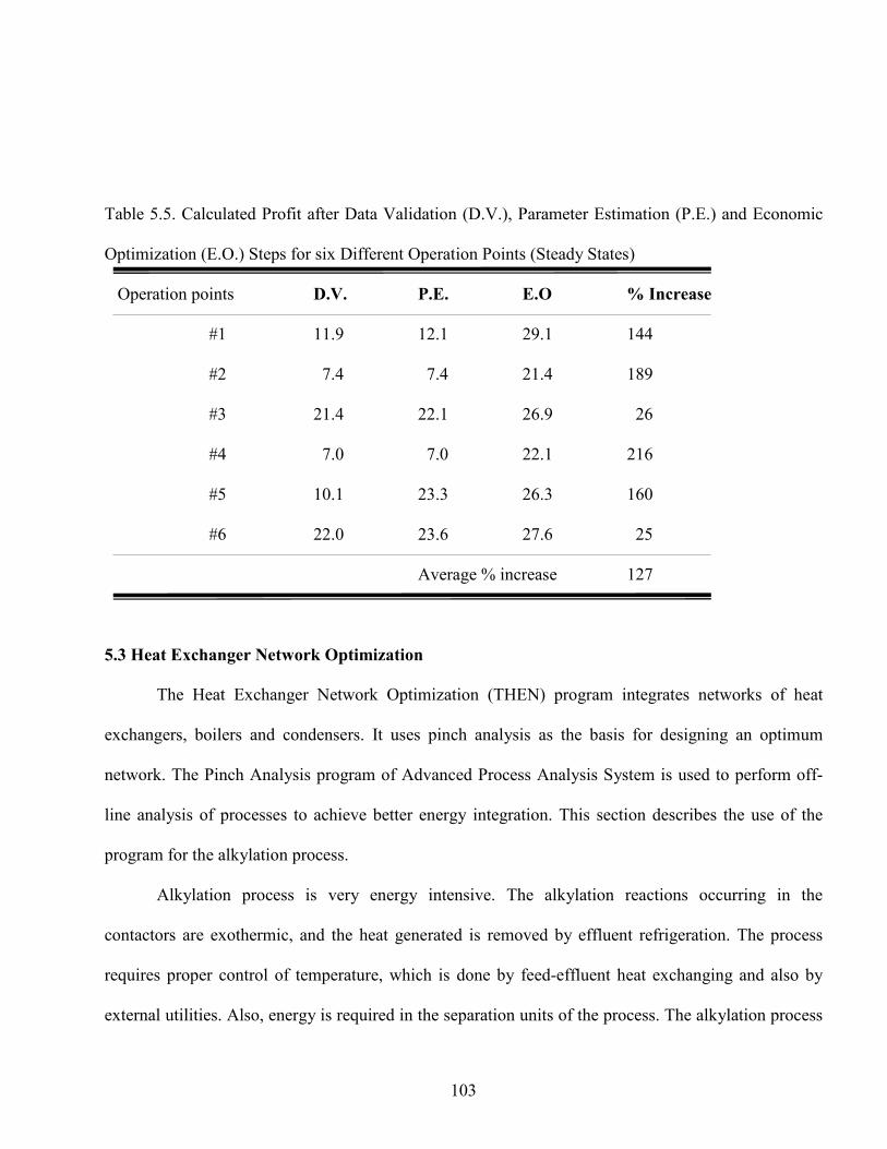
Table 5.5. Calculated Profit after Data Validation (D.V.), Parameter E timation (P.E.) and Economic
Optimization (E.O.) Step for ix Different Operation Point (Steady State )
Operation point D.V. P.E. E.O % Increase
#1 11.9 12.1 29.1 144
#2 7.4 7.4 21.4 189
#3 21.4 22.1 26.9 26
#4 7.0 7.0 22.1 216
#5 10.1 23.3 26.3 160
#6 22.0 23.6 27.6 25
Average % increa e 127
5.3 Heat Exchanger Network Optimization
The Heat Exchanger Network Optimization (THEN) program integrate network of heat
exchanger , boiler and conden er . It u e pinch analy i a the ba i for de igning an optimum
network. The Pinch Analy i program of Advanced Proce Analy i Sy tem i u ed to perform off-
line analy i of proce e to achieve better energy integration. Thi ection de cribe the u e of the
program for the alkylation proce .
Alkylation proce i very energy inten ive. The alkylation reaction occurring in the
contactor are exothermic, and the heat generated i removed by effluent refrigeration. The proce
require proper control of temperature, which i done by feed-effluent heat exchanging and al o by
external utilitie . Al o, energy i required in the eparation unit of the proce . The alkylation proce
103

model ha 28 heat exchanger , plu four pair of contactor . The heat exchange within the contactor
u ing the cold refrigerant conden ate through the tube bundle i not included in the pinch analy i
ince any new arrangement for the contactor will be impractical.
A di cu ed in Chapter 3, the fir t tep in u ing THEN i the identification of tream
important for heat integration. The e tream are the input and output tream to heat exchanging
unit . Appendix E contain the li t of tream from the model u ed for heat integration.
The econd tep i retrieving the required information for the elected tream, from the
optimization re ult . The data retrieved are temperature and flowrate a hown in the u er’ manual,
Appendix J. Energy calculation can be done either u ing con tant heat capacitie or pecifying
enthalpy coefficient for variable heat capacitie . To obtain average value for con tant heat capacitie ,
enthalpy of the tream hould be u ed and thi calculation i executed in the program a illu trated in
the u er’ manual. For variable heat capacitie , Appendice C.6 and C.7 contain the coefficient of the
equation u ed to evaluate the enthalpy for the component in the proce for ga and liquid pha e .
The temperature-dependent enthalpy equation u ed i a follow :
H = A0 + A1 T + A2 T2 + A3 T
3 + A4 T4 + A5 T
5 MJ/min (5.1)
From the enthalpy coefficient and tream compo ition , average enthalpy coefficient for tream are
calculated a :
Aavg = Σ AI xI (5.2)
where, AI and xI are the enthalpy coefficient and mole fraction of component I.
The third tep i cla ifying the tream a hot or cold tream . A mentioned in Chapter 3, a
hot tream i a tream that need to be cooled, and a cold tream i a tream that need to be heated.
The e are de ignated in the program a hown in the u er’ manual. Finally, the minimum approach
temperature for the network i cho en to be 13 K (See u er’ manual). Thi i to en ure ufficient
104

driving force between the tream in the network. The program u e thi information to conduct pinch
analy i for the alkylation proce by u ing the FORTRAN program THEN.
One of the re ult of the program i the Grand Compo ite Curve (GCC) hown in Figure 5.1.
Thi diagram how the temperature a a function of enthalpy for a compo ite of the tream . The
region of the GCC with a po itive lope how the proce egment that require energy, wherea the
region that ha negative lope how the egment that reject heat. The end point of the curve give
the minimum value of external heating and cooling required by the proce .
According to the Pinch Analy i the alkylation proce require a minimum of 1742 MJ/min
external heat and 4043 MJ/min of external cooling. From the data validation re ult , the current
external utility requirement are 1907 MJ/min of heat and 4300 MJ/min of cooling. The economic
optimization decrea e the heating requirement by 1% to 1888 MJ/min wherea the initial pinch
analy i reduce it another 7.7%. The cooling requirement can be reduced a much a 7.4% by u ing
pinch analy i from 4367 MJ/min after economic optimization. Thi i becau e the economic
optimization re ult in a 1.6% higher cooling requirement than the current value of 4300 MJ/min.
Figure 5.1 Grand Compo ite Curve for Alkylation Proce
105
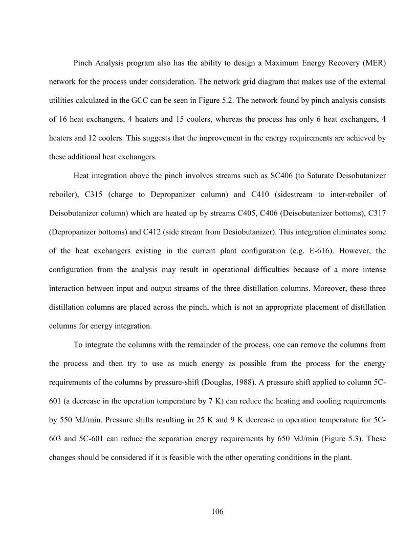
Pinch Analy i program al o ha the ability to de ign a Maximum Energy Recovery (MER)
network for the proce under con ideration. The network grid diagram that make u e of the external
utilitie calculated in the GCC can be een in Figure 5.2. The network found by pinch analy i con i t
of 16 heat exchanger , 4 heater and 15 cooler , wherea the proce ha only 6 heat exchanger , 4
heater and 12 cooler . Thi ugge t that the improvement in the energy requirement are achieved by
the e additional heat exchanger .
Heat integration above the pinch involve tream uch a SC406 (to Saturate Dei obutanizer
reboiler), C315 (charge to Depropanizer column) and C410 ( ide tream to inter-reboiler of
Dei obutanizer column) which are heated up by tream C405, C406 (Dei obutanizer bottom ), C317
(Depropanizer bottom ) and C412 ( ide tream from De iobutanizer). Thi integration eliminate ome
of the heat exchanger exi ting in the current plant configuration (e.g. E-616). However, the
configuration from the analy i may re ult in operational difficultie becau e of a more inten e
interaction between input and output tream of the three di tillation column . Moreover, the e three
di tillation column are placed acro the pinch, which i not an appropriate placement of di tillation
column for energy integration.
To integrate the column with the remainder of the proce , one can remove the column from
the proce and then try to u e a much energy a po ible from the proce for the energy
requirement of the column by pre ure- hift (Dougla , 1988). A pre ure hift applied to column 5C-
601 (a decrea e in the operation temperature by 7 K) can reduce the heating and cooling requirement
by 550 MJ/min. Pre ure hift re ulting in 25 K and 9 K decrea e in operation temperature for 5C-
603 and 5C-601 can reduce the eparation energy requirement by 650 MJ/min (Figure 5.3). The e
change hould be con idered if it i fea ible with the other operating condition in the plant.
106

From the Pinch Analy i , three loop and one path in the heat exchanger network can be
located. The e provide additional degree of freedom for further optimization of the y tem by
eliminating ome of the exchanger within the loop or on the path.
In ummary, Pinch Analy i provided an exten ive in ight for the optimization of the energy
con umption in the alkylation plant and howca ed the benefit of heat integration for the proce .
Figure 5.2. Network Grid Diagram for Alkylation Proce
107

400 400
350 350
300 300
280 280 0 400 800 1200 1600 2000 0 400 800 1200 1600 2000 MJ/min MJ/min
Figure 5.3. Integrating column (5C-601 and 5C-603) with the proce : Pre ure
hift for column 5C-601 only (left), for both column (right).
C601 C601
108

5.4 Pollution Assessment
Pollution A e ment program i u ed to a e the pollutant generated in the proce and
determine the location where they are generated. Thi information i u ed to modify the proce for
wa te minimization. Al o, a pollution index i evaluated for compari on of different proce e . In the
fir t tep of the program, input and output tream of the proce are pecified a hown in the u er’
manual, Appendix J.
The alkylation proce ha 10 input and output tream a li ted in Table 5.6. The e tream are
elected from Flow heet Simulation. The output tream are cla ified a product and non-product. For
example, pent acid (AC45) i a non-product wherea alkylate (C407) i a product tream. The
component pre ent in each of the e tream are pecified and the flow rate and compo ition of
tream are obtained from the re ult of On-Line Optimization program. The program’ u er manual
de cribe the e tep in detail.
Table 5.6. Input and Output Stream in Alkylation Proce .
Stream De cription Type Pollution Index
AC02 Fre h Acid Feed Input 0.808
HC01 Olefin Feed Input 1.622
SC414 Make-up I obutane Input 1.611
SC401 Sat-Dei obutanizer Feed Input 1.789
AC45 Spent Acid Non-Product 1.034
C320 To LPG Storage Product 0
C328 To Fuel Ga Product 0
C407 To Alkylate Storage Product 0
C413 To N-butane Storage Product 0
SC405 To N-butane Storage Product 0
109

A di cu ed in Chapter 3, pollution impact i calculated u ing pecific environmental impact
potential (SEIP) of the component in the tream . SEIP value of the component in alkylation
proce are li ted in Appendix G. Relative weighting factor for the nine categorie of impact were all
a umed to be one in the ab ence of actual value . U ing the SEIP value and relative weighting
factor the program calculate pollution indice for each input, product and non-product tream in the
proce , caling the effect of the tream to the environment. The e value are u ed to calculate the ix
pollution indice for the proce , which are li ted in Table 5.7, before (BEO) and after (AEO) the
economic optimization of the proce . Negative value mean that the input tream are actually more
harmful to the environment than the non-product if they are not proce ed through the alkylation
proce .
Table 5.7. Pollution A e ment Value for Alkylation Proce before (BEO) and after (AEO)
the economic optimization.
Index Type Value
(BEO) (AEO)
Total rate of impact generation -4.9120 -4.7966 impact/time
Specific impact generation -3.2860 -3.4584 impact/product
Pollution generation per unit product -0.9777 -0.9742 ma of pollutant/ma of product
Total rate of impact emi ion 1.0325 1.0337 impact/time
Specific impact emi ion 0.6897 0.7453 impact/product
Pollutant emi ion per unit product 0.1069 0.1154 ma of pollutant/ma of product
Pollution A e ment re ult how that the economic improvement that i achieved by the
economic optimization doe n’t come with a reduced environmental impact. The plant operating at the
optimal et point emit more pollutant ince the rate of impact generation i reduced, although
pecific component’ con umption might be le (e.g. ulfuric acid con umption i reduced by 2.2%).
110
5.5 Summary
Advanced Proce Analy i Sy tem wa applied to the Motiva alkylation plant. The proce
model wa developed u ing Flow heet Simulation program. On-Line Optimization wa u ed to
generate optimal et point for the di tributed control y tem. Pinch Analy i program wa u ed for
energy integration and to determine the minimum heating and cooling requirement . A pollution
a e ment of the plant wa made to determine the ource of the pollution generation.
111

CHAPTE 6
CONCLUSIONS
Alkl tion process is one of the most import nt refinery processes for producing
convention l g soline. This project demonstr tes process control nd modific tion
improvements to this process with Adv nced Process An lysis System th t employs
process flowsheeting, on-line optimiz tion, pinch n lysis nd pollution ssessment.
Also, the chemic l re ction n lysis p rt of the System w s used to determine the best
lkyl tion re ction kinetics.
Using the flowsheeting c p bility of the Adv nced Process An lysis System
simul tion of the lkyl tion process w s developed th t consist of 76 process units, 110
process stre ms, 1579 equ lity nd 50 inequ lity constr ints with 1634 v ri bles. The
simul tion w s v lid ted using pl nt d t nd d t reconcili tion to show th t the
simul tion predicted the perform nce of the pl nt within the ccur cy of the d t .
The n lysis of the pl nt d t resulted in detecting six ste dy st te oper tion
points. For e ch oper tion point gross errors were detected, d t were reconciled,
p r meters were upd ted nd economic lly optimum setpoints re determined for the
distributed control system.
The economic optimiz tion of the process for six oper tion points resulted in
25.4% to 215.4% incre se in the profit. As n ex mple; the profit for the process w s
c lcul ted to be $29.11/min, which is n incre se of 144.6% over the oper ting
condition (#1). This improvement in the profit is c used by 8.5% reduction in costs nd
2.2% incre se in s les. The economic lly optimum solution results in 5.5% more olefin
ch rge, lmost 100% reduction in isobut ne purch se cost, 7.2% reduction in s tur te
feed to the S tur te Deisobut nizer column nd 2.2% incre se in the lkyl te. The
112

lkyl te qu lity did not ch nge t the economic lly optim l oper tion. Energy s vings
tot l n ver ge of 9.4x10⁹ BTU/yr. This mount corresponds to 0.16% reduction in the
utility cost nd results in s ving of $5600 /yr. Another result obt ined from the
economic optimiz tion of the lkyl tion process is 2.2% reduction in the sulfuric cid
consumption.
According to the Pinch An lysis the lkyl tion process requires minimum of
1742 MJ/min extern l he t nd 4043 MJ/min of extern l cooling. From the d t
v lid tion results, the current extern l utility requirements re 1907 MJ/min of he t nd
4300 MJ/min of cooling. The economic optimiz tion decre ses the he ting requirement
by 1% to 1888 MJ/min where s the initi l pinch n lysis reduces it nother 7.7% (
tot l of 67x109 BTU/yr). The cooling requirement c n be reduced s much s 6% (
tot l of 106x109 BTU/yr). by using pinch n lysis . A further reduction in the energy
requirements c n be chieved by n ppropri te pressure shift pplied to distill tion
columns ccounting m ximum reduction of 650 MJ/min (268x109 BTU/yr).
Pollution ssessment of the lkyl tion pl nt reve led the extent nd loc tion of
the pollut nt emissions of the process. It h s lso shown th t the economic lly optim l
solution c n result in higher over ll pollution levels even if the consumption of the
sulfuric cid is reduced.
113

REFERENCES
Albright, L. F., 1990a, Modern Alkylate - 1:Alkylation will be key process in reformulated gasoline era, Oil and Gas Journal, 88, no. 46, 79-92
Baker, J. R., R. J. Hossli, M. M. Zanoni and P. P. Radeciki, 1995, A Demonstration Version of The Clean Process Advisory System, Paper No. 8a, AIChE Summer National Meeting, Boston
Ballinger, G. F., R. Banares-Alcantara, D. Costello and E. S. Fraga, 1994, epee: A Process Engineering Software Environment, Computers Chem. Engg., Vol. 18, Supp. P. S283-S287
Bernado N., M. Mazzotti, G. Storti, and M. Morbodelli, 1998 Multicomponent Distillation Design through Equilibrium Theory, Ind. Eng. Chem. Res., 37, 2250-2270
Brook, A., D. Kendrick, A. Meeraus, 1998, GAMS- A User’s Guide, Release 2.25, The Scientific Press
Cabezas, H., J. C. Bare and S. K. Mallick, 1997, Pollution Prevention with Chemical Process Simulators: The Generalized Waste Reduction Algorithm, Computers Chem. Engng., Vol. 21, Supp. p. S305-S310
Chen, X., 1998, The Optimal Implementation of On-Line Optimization for Chemical and Refinery Processes, Doctoral Dissertation, Louisiana State University, Baton Rouge, LA
Corma, A. and A. Martinez, 1993, Chemistry, Catalysts and Processes for Isoparaffin - Olefin Alkyalation: Actual situation and Future trends, Catalysis Reviews: Science and Engineering, 35, no. 4, 485-523
Cupit, C. R., J. E. Gwyn and E. C. Jernigan, 1961, Catalytic Alkylation, Petro/Chem Engineer, 33, no. 47
Cupit, C. R., J. E. Gwyn and E. C. Jernigan, 1962, Catalytic Alkylation, Petro/Chem Engineer, 34, no. 49
Douglas, M. James, 1988, Conceptual Design of Chemical Processes, McGraw-Hill, Inc.
Gary, H. James and H. E. Glenn, 1984, Petroleum Refining, Second Edition, Marcel Dekker, Inc.
Graves, D. C., 1999, Acid consumption and acid runaway on a sulfuric acid alkylation unit, Alkylation Seminar in Scottsdale, Arizona.
114
Gruse, W. A. and D. R. Stevens, 1960, Chemical Technology of Petroleum, Third Edition, McGraw-Hill, New York
Gundersen, T. and Naess, L., 1988, The Synthesis Of Cost Optimal Heat Exchanger Networks, Computers Chem. Engng., Vol. 12, No. 6, p. 503-530
Hegde, S. C., 1999, Simulations for Pollution Prevention, Master’s Thesis, Lamar University, Beaumont, TX
Heijungs, R. (Final Ed.); Guinee, J. B., Huppes, G., Lankreijer, R. M., Udo de Haes, H. A. and Sleeswijk, A. W., 1992, Environmental Life Cycle Assessment of Products Guide - October 1992, Centre of Environmental Science, Leiden
Hilaly, A. K. and Sikdar, S. K., 1994, Pollution Balance: A New Methodology for Minimizing Waste Production in Manufacturing Processes, J. Air and Waste Manage. Assoc., Vol. 44, p. 1303-1308
Hohmann, E. C., 1971, Optimum Networks for Heat Exchange, Ph.D. Dissertation, University of Southern California.
Kister, Distillation Design, McGraw-Hill Publishers
Langley, J. R., 1969, The Kinetics of Alkylation of Isobutane with Propylene Using Sulfuric Acid Catalyst, Doctoral Dissertation, Louisiana State University, Baton Rouge, LA
Langley, J. R. and R. W. Pike, 1972, The Kinetics of Alkylation of Isobutane with Propylene, AIChE Journal, 18, no. 4, 698-705
Lee, K.F., A. H. Masso and D. F. Rudd, 1970, Branch and Bound Synthesis of Integrated Process Design, Ind. Engng. Chem. Fundam., Vol. 9, p. 48-58
Linnhoff, B., D. R. Mason and I. Wardle, 1979, Understanding Heat Exchanger Networks, Computers Chem. Engng., Vol. 3, p. 295-302
Masso, A. H. and D. F. Rudd, 1969, The Synthesis of System Designs. II. Heuristic Structuring, AIChE Journal, Vol. 15, p. 10-17
McBride, B. J., S. Gordon, M. A. Reno, 1993, Coefficients for Calculating Thermodynamic and Transport Properties of Individual Species, NASA Technical Memorandum 4513
Perry, R. H., Green, D., Malony, J. O. (editors), 1984, Perry’s Chemical Engineers’ Handbook, Sixth Edition, McGraw-Hill International Publishers
Petrol.Refiner., 1952, 31 (9), 156-164
115

Rosenwald, R. H., 1978, Alkylation, Kirk-Othmer Encyclopedia of Chemical Technology, Third Edition, John Wiley & Sons, New York
Saleh, J. M., J. R. Hopper and R. E. Walker, 1995, Three-Phase, Catalytic Gas-Liquid Reactors: An Interactive Simulator, Paper No. 73d, AIChE Spring National Meeting, Houston.
Shaney, Agnes, 1995, Cleaner by Design, Chemical Engineering, Vol. 102, No. 7, p. 32.
Shenoy, U. V., 1995, Heat Exchanger Network Synthesis: Process Optimization by Energy and Resource Analysis, Gulf Publishing Co., Houston, Texas
Smith, B. D., 1963, Design of Equilibrium Stage Processes, McGraw-Hill Book Company, Inc., New York.
Telang, K., 1998, Advanced Process Analysis System, Master’s Thesis, Louisiana State University, Baton Rouge, LA
Templeton, P. C. and B. H. King, 1956, paper presented before the Western Petroleum Refiners Association, June 21-22
Thomas, C. L., 1970, Catalytic Processes and Proven Catalysts (McGraw Hill Book Company, New York), pp. 87-96
Van Reeuwijk, P. A., R. Zwart and M. E. J. Dreissen, 1994, CAPE in the Development of an Energy Efficient Chemical Process, Computers Chem. Engg., Vol. 18, Suppl. P. S161-S164
Vichailak, M., 1995, Pollution Prevention by Process Modification, D. E. Field Study, Lamar University, Beaumont, TX
Warren L. McCabe, Julian C. Smith, Peter Harriott, 1993, Unit Operations of Chemical Engineering, Fifth Edition, McGraw-Hill, Inc.
Winter, Peter, 1992, Computer Aided Process Engineering: The Evolution Continues, Chem. Engng. Prog., Vol. 88, No. 2, p. 76-83
Yaws, C. L., 1999, Chemical Properties Handbook, McGraw-Hill Handbooks, New York
Yongkeat, S, 1996, The sulfuric Alkylation of isobutane with light olefins, Master’s Dissertation, Lamar University, Beaumont, TX
Young, D. M., 1999, Personal Communication
116

117