FINAL REPORT

ON

A STUDY OF THE 1976-1980

NORTH DAKOTA RAINFALL ENHANCEMENT

PROJECT

By

Amos Eddy

December 1981

Done under the AMOS EDDY, INC. contract with theNorth Dakota Weather Modification Board

Dated September 1980

ABSTRACT

Evidence continues to increase supporting the conclusion

that cloud seeding in North Dakota produces an increase in

growing season rainfall which is significant both statistically

and economically. State average rainfall volume increases of

about 15% during the critical period from June 6 - July 11 are

found. This is produced by an increase in the number of

stations reporting rain in and downwind from the seeded areas,

combined with an increase in the average rain which falls in

each gage. No significant changes in the rainfall character­

istics are found beyond 12 hours downwind of the seeding.

Economic benefits for the state agricultural industry are of

the order of tens of millions of dollars annually.

i

TABLE OF CONTENTS

Page

ABSTRACT. . . . . . . . . . . . . . . . . . • . . . . • . . . • . . . . . . . . . . • . . . . . . i

A. INTRODUCTION. . . . . . . . . . . . • • • • • • • • • • . . . . . • . . . . . . . . . 2

B. ANALYSIS AND EVALUATION: THE PROBLEM............ 9

1. The Natural Variability............ 92. A Statistical Model of Rainfall.............. 18

C. ANALYSES AND EVALUATIONS: THE RESULTS... 21

1. One Day-A'LL Stations Analysis and EvaluationMethodologies. . . • . . • . . • . . • . . . . . . . . • . . . . . . . . . 21

2. Results...................................... 213. The Evaluation............................... 374. The Search for Treatments and Covariates..... 40

D. IMPACT........................................... 56

1. Drought In North Dakota......... 56

a. Soil Moisture............................ 61b. Evapotranspiration....................... 63c. Crop Moisture Index...................... 65d. Growing Season Soil Moisture and

Evapotranspiration............. 67e. Modelling The Data........... 67

2. Economic Impact.............................. 86

REFERENCES. . . . . . . • • . . . . . . . . . . . . . . . . . . . . . . . . . . . • . . . . . . 95

1

2

A. INTRODUCTION

The purpose of this report is to present an on-going

evaluation of the capability of the North Dakota Weather Modifi-

cation Board (NDWMB) cloud seeding activities to increase

rainfall where and when it is needed across the State.

Previous work done for the NDWMB by the author and his

colleagues considered the period up to 1976 and compared the

climatology of rainfall before seeding began (circa 1950) to

that which was reported after seeding of one sort or another

was undertaken somewhere in the State. The post 1950 rainfall

enhancement was assessed rather crudely using: a) some 59

National Weather Service (NWS) daily cooperative observer reports,

b) documentation as regards which counties were "in" and "out"

of the seeding activities each year, and c) the mid-tropospheric

wind reported at Bismarck each day to define downwind pro-

gression of a "seeding plume". A significant rainfall increase

associated with this "seeding" was found over most of the

State and the results are reported in detail by Eddy and Cooter

(1979) and Eddy, Cooter, and Cooter (1979).

Beginning in 1979, we used refined observation networks

and trajectory calculations to define:

a) exactly where, when, and how much seedingwas released into the atmosphere,

b) a special 500-600 gage network of rainfallobservations, and

c) a more sophisticated computer algorithmwhich makes use of all upper air data inand around the State to calculate the

3

downstream trajectories of the seedingmaterial (Heffter and Taylor, 1975).These latter trajectory calculations areperformed by Dr. E. R. Reinelt of theUniversity of Alberta in Edmonton. Thiswork is reported in detail by Eddy (1980).

During the past year we have concentrated on the 5-year

period from 1976 to 1980. The present report describes our

results concerning: a) rainfall increases (and decreases) in

and downstream from seeded areas, b) changes found in the

characteristics of this rainfall, c) the statistical signifi-

cance of these changes, d) variations in the thermodynamic and

kinematic structure of the atmosphere associated with these

changes, e) hypotheses Of expected changes found using a simple

cloud physics "cloud seeding" model, f) economic impacts of

the observed changes (rainfall increases), and g) a background

study of drought frequency and intensity across the State of

North Dakota, done to begin an assessment of the rainfall en-

hancement possibilities during such anomalous weather regimes.R

Figure 1 shows the long term (~O years) average annual

rainfall pattern for North Dakota. This is based on the

NWS COOP data set which ranges from a few stations in the early

years to well over 200 in more recent times. Figure 2 shows

the special rain gage network distribution by county for one of

our 5-year study years and Figure 3 shows the special network

distribution for another year in some detail. These stations

move to a certain extent from year to year; however, the basic

station density remains the same. Figures 4 and 5 show the

counties which have contracted for cloud seeding in each of these

5 years. These latter two figures show the position of our upper

air observing station at BIS (Bismarck).

,.~' ..~ ..: ': ........... ::...- .........."'e", ....

lq"

.c-

I!S"

," ~ ," : : .. n... . ,'; :: " .... ... .. \ . . 'O.... :"..... p,.: -, .... .... .. ...

:J . •", .\.

- ... .. ..: .", " : ... 'O."

':,,:':/:::.~:.... ."..' ~ ....

". '" " ..'O. .'O.'..... , ...: "~ .. :'O ..." "'., ..........., ,", '.:. . :. .. -.

I. . .'' .... .,. ".:-':'" ~." ".~ -~...""

Figure 1: Long-term annual precipitation over North Dakota. Mean = 16.8",spatial standard deviation of station long-term means = 2.04".Approximately 16% of the state receives over 19" (hatched area) and16% of the state receives under 15" (stipled area) during the"average" year.

!

Divide Burke I RenvilleI Rolette Towner Cavalier

\ Pembina

Bottineau

9 7 (~7 4 r; 5 E 4 ~

1.J

1t

Williams McHenry \ Walsh

l lpierce

f

Mountrail

Ramsey

6Ward '1 6

Benson .1.-

23 23 10 7~JNol.an \LArJ

Grand Fork.

\15

Me KenZie I I 12 6

~t McLeanJSheridan1wells

EdGY

ll37

\,

~ 26Traill

GriggS Steele

Dunn ~ G 15 Foster

~Mercer 5 3 5 8

l l! 9~

Golden Billings Bur!e H;)h Kidder Stutsman

Valley OliverBornes

ce s s V1

611 6 11 11 17 30 7 1

stork Morton

10 11

I

I

--.lsiape-S-Emmons

RansomRict.la nd

Heltlngerlooon La Moure

Grant \11 10 .-'\ Q 6 13 8

I 12 10 sargent

1Bowman AdamsSioux

\Me Intosh

Dickey

0 10 ~ 58 10 12

o

1978 RAUl GAUGE HETHORK DISTRIBUnDti BY COUnTY(APRIL 1 - SEPT. 30)

FIGURE 2

•..................................................................... .. ..-.- ....... '".-

I

a;

•

•

•

•

•

•

••

•

••

•

••

•

•

••

•••

•••

•

1

1

1

1

1

1

11

1

11 1

1 1

1

3

1

1

I

1

I I 11 I I

11 111

11I

1 1 I 11

I 1I

I

I1

I 11111 31

I1 1 I

1 II 1 11 1

I

1 1

11

1 I

1 IlJl1 I,

I I

11

1 I 1 1I 1 1

1

11I

II

11

1

I

1

1

1

11

I111

1

1

1

1

I,

I

21

I1

I1

1

1

12

I

I

I 1

111 I

1

I2

I2

I2I

I 1

11 1

I

1111

1

2 I

2 II211

11 I1

IIII I

I

1 1111 1'I

I I

I

1 I I1

1

1I

III

11

1

1 II

1

1

2I

I

II

II

1

111

1

I I

I

I

1 2

II

I

I

1

I

'.

I

I1

11

1 II 2

I

I

III 2~1211 1

2 I

1 I 1 I.. "",

1 I Ll 1

1

I

I1

I

2

1 II

1211

11

1

I

12 1

1

1

11 I

1

I II2 II I

II I III

2

1

1I

1I 12

III1

1

1

I Ir

I I I11

I11 11

II

II

1

1

I I II

I I 1I 1

I II I

I

III

I2

;;

1 2

21

1I

"

I

1

~ 1 '1~I I

I

111 2

1 1I 1 1

1

1

I

I 1

II

I III

II

2

1

•

21 I

I

I

I

I 1I I

I11I 1

I I1 1

I 12I

I

I

1

II

I2

••

••

•

••

••

•••

••

••

•

Fig. 3. The' 1977 North Dakota daily rainfall observing ne t wor-k (coop net not included).areas shown

Project

I IMCH.n~ I.-~__--llPierce

.....,

\

)Riddand

Trail!

i pemutnc

Walsh

Dickey

Ramsey

La Moure

GovohetTowner

Mc Intosh

RoletteBottineou

Oliver

Renville

Morton

8urke

Stork

Divide

WiJlioms

GoldenVolley

Figure 4: 1976 seeding project area. The location of the rawinsonde station (R/S) is at Bismarck (BlS).

Olvid.Burke Renville Bollineou Ro/ells Towner Cavalier

Woi,hRomsey

1t: Wi"d . :" .•. : ••. --:~ ,

Williams

IShefldon ! We1l5 I Eddy

Billinos

\.I ! FoslerI I b r.rinCls ASleele Trolll

1COBBorne!

sr c t sm en

I '------'t ~I Burte Inb I Rl d d er

Oliver

GaldonVolley

OJ

Sior k Morlan BIS

Grant 1 Ernrnc n s LOQan Lo Moure Rc n so m Ric",lond

. ) .

/L-. .",-·-I~

Sioux ( Me Inlosh

I

Dickey Safoe ni

~

\

Figure 5: Seeding project areas 1977, 1978, 1979, 1980 shown shaded. During 1977 only, GRIGGScounty was also in project area III. The location of the rawinsonde (R!S) stationis at Bismarck (BIS).

9

B. ANALYSIS AND EVALUATION: THE PROBLEM

There have been two major thrusts to this problem:

i) to what extent have the rainfallpatterns been changed by the cloudseeding?

and, ii) what is the probability that theseanalyzed changes are real and notsimply "produced" by the techniquesof analysis?

In this section we present the methodologies we have used

to provide answers to each of these questions.

1. The Natural Variability

In order to test the significance of the difference between

seeded and non-seeded rainfall in the most effective manner, it

is helpful to remove natural sources of variability from the data

sets. Two principal sources of such variability derive from,

a) the tendency of rainfall to come from clouds associated with

different types of synoptic-weather systems, and b) within each

of these types: for there to be more or less atmospheric

moisture available, more or less lifting of the air to condense

such moisture, and other continuously varying properties.of a

similar nature. This section describes our search for ways to

discover these two sources of variability in an objective manner.

The first source «a) above) we call clusters, stratifications,

treatments or non-homogeneities. The second source we refer to

as covariates. Figure 6 shows some features of the long term

rainfall variability in the statewide average (non-zero) rainfall.

Stations reporting zero rainfall were excluded in this case.

The widths of the distributions shown are very roughly proportioned

I I 1951 1951 1913 !1951 11913 1951 1951 '1951 [\Years To To To To I To To To To

1976 1976 1976 ,1976 1948 1976 1976 1976'lind

1 Dir.

Seeding!;.rea

H =

Figure 6.

in:·!, H-'- All I All INV!, H I All I SH I S\,/ I SHSW Winds Winds I SW Hinds

Seed

7574

.2Q <2.1 -2.2 ·23 -24 -2..5 ·2iS -1.7 -2U ·29 -30 ·~l -32 ·33 ·34

Rain (inches)

Some North Dakota climatology: mean rain on a rainy day.Reports of zero rainfall at a station not included. 59cooperative network stations used.

......o

11

to their expected variability. Notice that the mean value for

the 96,692 non-zero rain reports found before 1951 is signifi­

cantly greater than that obtained from the 58,274 non-zero

reports taken after 1951. Since cloud seeding began about

mid-century in North Dakota, one might conclude that it had

decreased the rainfall. Such, of course, was not the case and

such a conclusion represents one of many ways in which one can

misinterpret rainfall analyses. In fact, the frequency of

non-zero rain reports is much greater after 1951 than before and

the net annual rainfall turns out to be about the same in both

eras. What one might profitably consider based on this simple

analysis is the possibility of a time change in the manner in

which the atmosphere delivers its rain to the state. Long-term

natural variability is suggested.

Significant irregularly occurring natural variability is

suggested in Figure 35. Although this figure shows a soil mois­

ture budget which also incorporates temperature affects, it shows

that one should expect, AT IRREGULAR INTERVALS, persistent

weather systems which deliver less than average or greater than

average rainfall. These intervals can range from a few months

to several years. Of course, on top of this variability we have

the REGULAR annual cycles such as are shown in Figure 32. Fig­

ure 6 also suggests that wind direction is an indicator of ex­

pected rainfall amount. Figure 7 bears this out and adds the

information that this directional effect is a function of season

of the year. Does wind direction change imply a continuous

variation in rainfall within a synoptic type and consequently be

considered a covariate? Or, does a southwest wind imply one

elf:'

I-'ro

--------- ...

-~.~.~~.--~~_._-

-- ... -.--_.... --­

.... ... ,,-.,.--......----

·35

.!le

,-- .... ,I 'I \

I 'I \, ', .,

I ', \ ,, \

I 'I ', ,

I ', \I '

I 'I "

I 'I ', . ', ", ", ""r ",,,,,-

~ I' . ,,'2 -!':!..",.I"

~ .15'J,w

<

~ .30'-':2;.-<

"., .• 25zH

~

25 .20

'-<:

~

­,,"' .. " .",,10 i NW('". I 1 I 2 I 3 I 4 II 5 I 6 I 7 I 8 ' 91 ' 10 I 11 i 12 i 13 114 I 15 I 16 I 17 1118 I 19

It.AY JUNE' JULY AUGUS':C

Figure 7, North Dakota mean rain on a rainy day as a function of wind direction and month.

13

weather type and a north wind another; consequently, should we

account for discontinuous changes in the mean (expected value)

in our analyses based on wind direction? More information is

needed!

Figure 1 showed a northwest-southeast gradient from dry

to wet in the annual precipitation averages across the state.

Figure 8 shows about the same pattern for a time interval during

the year which includes the cloud seeding season. However, when

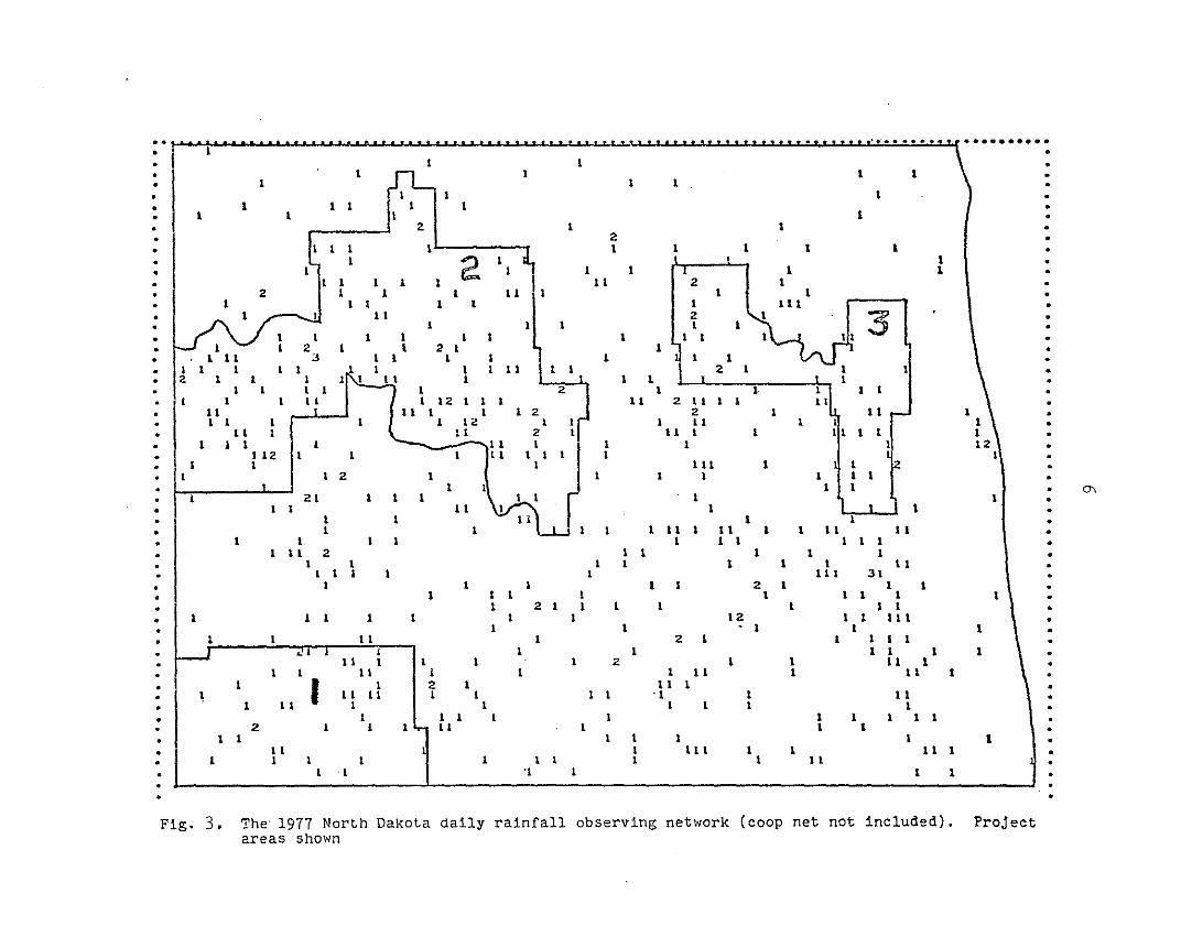
we check Figure 9 we find that the rainfall which occurs during

the critical June growing period imposes a much more chaotic or

random pattern on the general NW-SE trend. In fact, when Fig-

ure 9 is compared to Figures 4 or 5, one sees that the natural

long-term variability in space in the target areas and during

the critical few weeks of seeding activity is large enough to

be of some concern in our evaluation problem. It was for this

reason that we conducted our earlier analysis STATION by STATION

to obtain results such as those shown in Figure 10. In this

case we subtracted from each rainfall report (both seeded and

non-seeded) the long-term average value for the station at the

given time of year and for the given wind direction (COVARIATES),

in order to obtain DETRENDED rainfall values. We averaged the

detrended seeded rainfall values and from this we subtracted the

average of the detrended non-seeded rainfall values to obtain the

results shown. Another presentation of this same type of analysis

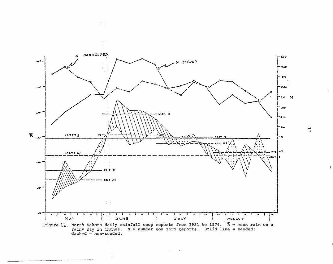
is given in Figure 11. This shows anotl1er type of variability

which permitted us to find a positive seeding effect only in tl1e

June and early July period.

f-'.c-

i

...

.... .. ....: .. ,. .".. .>-

~: : ~ ":- ....... , ..: ..".:" ~,'...... :

.. ".. .... ..... .... .... .. .. ' ... '.'t" .. to.. ",.".. ."............ : ..

.... .... ..­.. .. ,..".... ' ...

.. ' .. .'.. - a ... • ,

"I .. ",", ........~.. " .. .. .. " .."'.. .. ... .. " '-." .... .. .. ... .. ..", ' ; .... or: .... ... ~ .

.,. ., ...... I ~ "' .". ", ---........- .. ...,............",~:·"W'·"':f.'~.

, .

Figure 8: Long-term mean precipitation over North Dakota for period April 1 ­September 15. Mean = 12.3", spatial standard deviation of stationlong-term means = 1.47". Approximately 16% of the state receivesover 14" (hatched area) and 16% of the state receives under 11"(stipled area) during this 24-week period On the average.

®

~

~" " '•.

"," ~ ...... '..'.

':t~·~'~·,:::~:~·: ·':0'~.~:'.::':.I{ ,::: : .::.~I~'" " ... ",:, .. .. .. " .."" .. .. .. " ~ ( ..': •• < :.:,: •• '

.." .. ", ~ .. .' ...:,:.::.:::: .. , .

l-'V1

/.1a

Q ~

~t9

~

&

~

@D-'"..." ....-

~

~

Figure 9: Long-term mean precipitation over North Dakota for period June 6 ­July 11. Mean - 3.88". The stipled areas receive less than 3.5"and the hatched areas more than 4.5" during this 6-week period onthe average.

l~lt.

a·1H·l0,+50

B

AtC

l

\1 38

1·26;;·03276

Station!(odel

t-'

6' 0\5·15*··051

1 6 3

\

)

.1366·8*-007

, 5

1266'63*'051

82

345.52*.041

81

11 35"4*-'001

84 1256·57 ",-.os

1 0 0

13 ,1.3 *-.022

88

114 •6*-.061102

224alf

o

1467.·68*·044

48

1421·47l!·02'

53

814·05""013

'9 1304 • 95* • 016

78

1668·3;\-·011

100

113S .. 9 ~.~ .. 0 1 6

e 4

1 3 5j'·94*-OU6

1 17

1 9 5'.75*-.0.11 10'

2 3 6 • 8 1 *-. 0 24 a

20612.11*-0.124

17

1 347.44p.123

73

1299 1 6 .. It 5 ~ .' 1 1 ,

5'4*'028 111111·

1189.36~.116

451 5 a

"29,,'0:73 5

11 86"4*-·04

125 1337 .. 81*-.0-56

82

'715·07*·067

1 6 3

1 539 .. 55* .. o~s

21

1 0 36-431:,,02

87 .119124 6• 2 6¥..075

7. 2 3 11 · 0 6 2 9 035

.. -'" -~,-' ,, \

151 <127 I, .. 11 3 J! .. 0 S 5 ••6 .. It 6 *- .. 0 0 e I

70 # 78 ~. 'I '

-/ ~'I ,

I 'I •!

.17311' 53*-' 011

6 5

20 5169 12·051\·04

12·07* • 044 292 2 3

70 13.47*-.0.1122

1 3 0,'281\-'004

51

1 52, • 5* • 0 32

11 0

1 4 410'28,,'05'

124

£­182

1'212*'116

37

To230

15 213·8 ",-.008

"78

I

i

*1 9 ,

5511*'014

, 6

I

I1 2 6

8 .... r. ". 0 4. S 1 S -4

27 "641"0543 1

Figure 10. North Dakota seeding statistics 1951-1976. Station model:A = mean number seeded rainy days per season (June 6-July 11)B = Total number in seeded sampleC = (seeded - non-seeded) mean rain on a rainy day (inches)D = total number in non-seeded sample.

f--'.....,

N

1'00

1:00

;"00

r--..........,- ',- ./

"'...... "'-':;-,,'"~

..,z./ N -;';/:"1>",1>

.1'--,// -0..... ......

'\ J /7--...../ ~/'....-~v..... <'

''':57:5' S

N Non SerE;;>!;]>

,,~tJ"" "

'"--......"'\

'\.u"

I~~I

....

..,

...

I tx",

h"

.",-'"'' I" ,\\'~ ~,o.

..>r '\\\,:~.v ; vy:~ -, ../. . _>1('~\\"" .::;-~",,=,--... 1'00

___ "",., I" --'0',,;; ..., ~,. ,______ f' - ,. -~' -, A .'

.&

.,,-_________ '\ ,_"'" '" ...t- r'• ,.. " ..\~/.. \ I

I \\\ r: ----- . ", t r ::'" ," ~ L-e ...\

~__ 6:,1'1:'"-\ .,: ,,,.. 't":,:C: :; :"~:C±'-IH'.t; "",,,"'-V '" ,,; 1\ ,~.«"" ,if)-"" ----0" ~ V " V\Y' 'v '

'''1 ' j -. I > I • I !r I , I , J • J 'I 1 ,. J " I 'L I " I .. j .r J .. I .. ( I~MA.Y .:rUN!: :rUL..Y ACG"u..ST

Figure 11. North Dakota daily rainfall coop reports from 1951rainy day in inches. N = number non zero reports.dashed = non-seeded.

to 1976. R= ~ean rain on aSolid line = seeded;

18

2. A Statistical Model Of Rainfall

The rainfall observations on which we base our analysis

and evaluation are made once per day at 0700 in the morning

local time. Thus, our basic experimental time unit is one day.

The distribution across the state of our gage network makes our

basic experimental space unit about 100 mi 2 • Since a consider­

able amount of the rainfall in the state comes from cloud systems

which are smaller than this space-time mesh size we will have to

rely more heavily on the statistics of many cases than would be

necessary if we could analyze the rain producers cloud by cloud.

Furthermore, since we are assessing a non-randomized

operational program we must rely on the NATURAL RANDOMIZATION

produced by variations in seeding location and wind direction

to produce our seeded and non-seeded samples. This means that

we must wait longer to obtain our adequate sample than would be

the case had randomized cloud seeding been used. The sample

size required to make a definitive evaluation is implied by

Figure 12.

We want to group into clusters the observations made for

each separate population, or synoptic weather type. Then we

need enough observations of covariates and rainfall within each

weather type to enable us to reduce the natural variability and

average out the noise to the point where the expected difference

between seeded rainfall and non-seeded rainfall stands out

clearly. Since these expected differences can themselves vary

from one weather situation to another, we need the assistance

of quantitative cloud physicists to help stratify our data sets.

19

A RAINFALL MODEL

RESPONSEVARIABLES

RAINFALL

RADARREFLECTIVITIES

CTT

= AT

TREATMENTS

SEPARATEPOPULATIONS

NONHOMOGENEITIES

DIFFERENTSEEDINGTREATMENTS

DIFFERENTCLOUD TYPES

SYNOPTICWEATHER TYPES

STATIONLOCATION

+

COVARIATES

COMMONINFLUENCES

WI'I'HIN­POPULATIONVARIABILITY

CBT

AMBIENTSTABILITY

WINDDIRECTION

+

NOISE

FIGURE 12

20

Once we find the needed TREATMENTS and COVARIATES, we proceed

as follows. From each rainfall observation (both seeded and

non-seeded) we subtract the treatment effect and the covariate

effect. This leaves us with two sets of noisy residuals: one

set for the seeded rainfall and one for the non-seeded rainfall.

If we have done our job right, the noise should be random and

tend to be averaged out as our sample size increases. If the

seeding effect is systematic and NOT random it will show up as a

progressively more distinct difference between the averages of

the seeded and the non-seeded samples the more reports we obtain.

The next section will show the progress we have made in this

direction over the past year.

21

C. ANALYSES AND EVALUATIONS: THE RESULTS

As discussed in section A, our principal work over the

past year has centered around the comparison of seeded with

non-seeded rainfall on a day by day basis for the five years

from 1976 to 1980 inclusive. The following section will

present the results from analyses using three data sets:

i) the 500-600 special rain gagenetwork across North Dakota(e.g. Figure 3),

ii) the seeding information pro­vided by the logs of the pilots,

iii) air trajectory information fromthe rawinsonde network in andaround the state.

The succeeding section illustrates our approach in

searching for weather types and covariates. It uses output from

the first section plus:

1) One-dimensional cloud model outputstatistics on the atmospheric thermo­dynamic and kinematic structure overNorth Dakota inferred from the BISMARCK,North Dakota rawinsonde observations.This (GPCM) cloud physics algorithm alsoestimates changes in the convectiveactivity which should result from cloudseeding based on an objective (butsimplistic) hypothesis.

1. "One Day - All Stations" Analyses And Evaluation Methodologies

Figure 13 has been abstracted from a computer printout show-

ing seeding locations and air trajectories for one day in the

North Dakota data set. The details of this procedure are described

extensively in Eddy (1980). Briefly, the aircraft used on this

day injected silver iodide in two main geographical-time clusters

Figure 13: Two seeding areas and downwind plumes found for one 24-hour period(0700 LST-0700 LST) over North Dakota. The centroid of the larger areawas found at 5,000 ft. and 2100 LST. The centroid of the smaller areawas at 6,000 ft. and 0700 LST. Rain gage reports for the same 24-hourperiod will be flagged to show the sector in which they are located.

NN

23

and we hypothesize that the wind bore this seeding material and

the cloud systems toward the northeast as shown. Rain gage re­

ports under the target areas were coded for the day as being in

sector 1. The gages in the areas downwind from these target

areas as far as the three-hour lines of demarcation (marked

2400 LST for the northern track and 1000 LST for the southern)

were coded as being in sector 2. Gages in sectors 3 and 4 were

similarly flagged. All gages lying outside any seeded sector

were flagged with a zero. Mean daily rainfalls and intensity

distributions were then calculated for each sector as well as

for the combination of all seeded sectors and finally for all

gages combined. We are now able to compare the seeded and non­

seeded rainfall averages as well as the distributions of intensi­

ties for the day.

At this juncture we are making the tacit assumptions that

(FOR THIS DAY) the entire state is in the same weather regime

(synoptic situation) and that the covariate values are the same

for the seeded as for the non-seeded rainfall. These assump­

tions are the counterparts in this all-space-at-one-time analysis,

of the trend removal assumptions described above (Figure 10) in

our previous all-time-at·-one-point analysis. The main confound­

ing influence on each day in our present analysis is the natural

variability across the state. This must be reduced by combining

many days with different wind directions and seeding areas. Be­

fore bringing about this combination we concern ourselves with

the possibility that the "seeding effect" itself may be greater

on days showing large statewide average rainfall than it is for

24

days with small statewide average rainfall. Because of this

possibility we transform the difference (d) between the seeded

rainfall, Rs and the non-seeded rainfall R according to thens

following formula:

d = (Rs

The precise formula for doing this is given on page 48.

It is these "d" values which we combine to assess the significance

of the seeding effect; whereas, it is the combined daily increase

(or decrease) which we use to assess the economic impacts.

2. Results

Table 1 shows the general overall statewide results for the

5-year period under study. This table implies the same kind of

results as were shown in Figure 11: the most effective rainfall

enhancement derived from seeding in North Dakota is to be found

during the six-week period from June 6-July 11. Table 2, however,

implies further that rainfall increases of lesser statistical

significance can be produced outside this period.

Another facet of the problem studied concerned daily rain-

fall intensity distributions in the non-seeded and seeded areas.

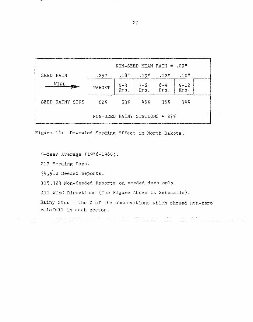
As can be seen in Figure 14, the gages in the seeded areas

tended to have higher daily rainfall values than did the gages

in the non-seeded areas. This could have occurred by there being

more rain per storm cell OR by there being more cells per day in

the seeded areas than outside these areas. The latter possi-

bility seems to be indicated by Table 3 which showed a higher pro-

portion of the gages reporting non-zero rainfall in the seeded

areas than was found in the non-seeded areas.

25

TABLE 1

--~-----------------------_._--

STATEWIDE ANNUAL AVERAGE VALUES (5-YEAR MEANS (1976-1980»

All Seeded Days During Season Total = 6.66"

Portion Attributed To Seeding During Season = .89"

Mean Percent Increase (Using All Seeded Days) = 15.4%

Mean Total Rain June 6-July 11

Portion From Seeding June 6-July 11

Mean Percent Increase June 6-July 11

= .50"

= 14 .. 2%

NOTE: In the above the 6.66" considers seeded days only;

whereas the 4.02" is all rain during the period of

major impact on spring wheat. Thus, the percent

increase on seeded days only during the June 6-July 11

period will be somewhat greater than 14.2%.

26

TABLE 2

,Tune 6 - July 11 For All Seeded Days in Year

Actual Rain 6R Actual Rain 6R NUl1 Seed Days. --

1976 3.67 .80 5.86 1. 34 70

1977 5.08 .67 7.20 .89 53

1978 5.59 .18 6.66 .51 47

1979 2.96 .29 6.12 .79 63

1980 2.79 .57 7.47 .94 63

11ean 4.02 .50 6.66 .89 60

14.2% Increase 15.4% Increase

For All 36 Days For Seeded Days Only

SUMMARY OF NORTH DAKOTA 5-YEAR RAINFALL MODIFICATION ACTIVITIES

27

NON-SEED MEAN RAIN = .09"

10"12"19"18"25" . . .

TARGET 0-3 3-6 6-9 9-12Hrs. Hrs. Hrs. Hr s .

SEED RAIN

WIND

SEED RAINY STNS 62% 53% 46% 36% 34%

NON-SEED RAINY STATIONS = 27%

Figure 14: Downwind Seeding Ef'fect in North Dakota.

5-Year Average (1976-1980).

217 Seeding Days.

34,912 Seeded Reports.

115,323 Non-Seeded Reports on seeded days only.

All Wind Directions (The Figure Above Is Schematic).

Rainy Stns = the % of the observations which showed non-zerorainfall in each sector.

TABLE 3

RATIOS OF NON ZERO RAIN COUNTS TO TOTAL COUNTS

(ON SEEDED DAYS ONLY)

NonAll Seed SeedRain Rain Rain Target 0-3 hrs 3-6 hrs 6-9 hrs 9-12 hrs 12-15 hrs_..... -

1976 .28 .23 .41 .52 .42 .32 .27 .41 .22

1977 .38 .31 .56 .67 .58 .54 .38 .32 .32

1978 .35 .28 .57 .75 .59 .47 .23 .34 .27

1979 .28 .24 .44 .58 .48 .41 .39 .27 .16•

1980 .35 .30 .55 . 60 .56 .55 .51 .37 .18

Mean .328 .272 .506 .624 .526 .458 .356 .342 .230 ro(X)

29

Lastly, the downwind effect was, in general, positive

(increased rainfall), with no seeding influence detected more

than 12 hours downstream from the target areas.

The year to year breakdown of the composite results

shown in Figure 14 are given in Table 4.

Another important piece of evidence to support a seeding

effect concerns changes in the rainfall intensities shown by

gage cbservations. Table 3 implied such a shift toward higher

24-hour rainfall amounts falling in seeded gages than in non­

seeded gages. Table 5 gives supporting evidence. Figure 15

shows this effect graphically for the 5-year period.

It is important to realize that seeded days tend to

produce more rainfall naturally than do non-seeded days, and, in

fact the distribution of rainfall on non-seeded days is differ­

ent from that of non-seeded rainfall on seeded days. Table 6

shows this result.

Why are non-seeded days different from seeded days?

Is the synoptic weather situation basically different? Many

of our non-seeded days occur in April and May before the field

programs begin; consequently, it is logical to suppose that the

spring rain producers differ from those of summer. It is also

the case that in spring the clouds are colder and the moisture

supply less (two reasonable covariates).

We have discovered that these differences in rainfall

intensity distributions produced by seeding tend to disappear as

the systems move downwind, and in fact disappear after about

12 hours. Figures 17-21 show this result.

30

TABLE 4

STATE tlEAN DAILY RAIN IN INCHES

(SEEDED DAYS ONLY)

Non Seed Seeded MeanAll Rain Rain Rain d Value Nd S.D. (d)

1976 .08 .06 .13 1.18 50 .14

1977 .13 .10 .23 .87 42 .15

1978 .14 .10 .24 1.13 36 .17

1979 .09 .08 .16 :1.14 40 .16

1980 .n .09 .22 .95 42 .15

Mean .110 .086 .196 1. 05 210 .07

NTOT 150235 115323 34912

Target 0-3 hrs 3-6 hrs 6-9 hrs 9-12 hrs 12-15 hrs

1976 .20 .10 .09 .08 .13 .04

1977 .25 .22 .28 .12 .09 .06

1978 .35 .23 .21 .11 .12 .02

1979 .24 .16 .14 .13 .06 .06

1980 .21 .21 .25 .18 .08 .07

Mean .25 .18 .19 .12 .10 .05

NTOT 8271 13470 8334 3174 1139 318

31

.01 - . 1 .1 - .5 .5 - 1.0 1.0 - MAX N

1976 30.0 48.6 15.3 5.9 4,589

1977 18.2 53.1 19.8 8.7 4,055

1978 14.6 52.9 22.1 10.2 2,894

1979 26.1 50.7 13.7 9.3 2,302

1980 22.2 50.3 18.6 8.8 3 781

Weighted 22.6 51.1 18.0 8.1 17,621Mean

Table 5a: Percent frequency of seeded rainfall - all sectors ­by year and intensity class .

.01 - .1 .1 - .5 . 5 - 1.0 1. 0 - MAX N

1976 35.96 46.20 14.05 3.79 6,682

1977 25.33 52.65 16.65 5.37 6,384

1978 28.12 44.38 17.79 9.72 4,261

1979 31.83 46.94 13.08 8.14 5,466

1980 27.91 51. 53 14.97 5.59 8.388

Weighted 30.00 49.00 15.00 6.00 31,181Mean

Table 5b: Percent frequency of non-seeded rainfall on seededdays by year and intensity class.

50

40(/)zoHE-<

~ 30[iI(/)

111o"" 20

10

32

1:'- - - - - - ••* •• .. ••.-.... .... .. .., ,-..... .. ..,; .. ;.... :," :.4:':... ., ...."

: ... I :. .... .,:. .....

.01" . 1 " .5" 1.0" MAX .

DAILY RAINFALL IN A RAIN GAGE

Percent frequencies in 4 rainfall intensity categories.

SOLID = seeded rainfall

DASHED = non-seeded rainfall

HATCHED areas show higher frequencies in seeded areas

STIPLED area shows lower frequency in seeded areas

Figure 15: All 5 years. All seeded sectors; non-seededrainfall on seeded days only.

33

TABLE 6

RAINFALL FREQUENCIES FOR ALL DAYS

APRIL 15 - SEPTEMBER 30, 1976 - 1980

Daily Rain All Non-SeededIntensity Non-Seeded Seeded Rain on

(inches) Rain Rain Seeded Days

O<R<.l .325 .226 .30

.1~R<.5 .500 .511 .49

.5<R<1.0 .131 .180 .15

1. O<R .044 .081 .06

N 74977 17621 31181

The seeded rain is also broken down as a function of downwindsector.

50

40(f)

z0H 30Eo<«:>p;::rx:I 20(f)

o:l0

"" 10

~34

..Total Sector 1 Count

.. = 5,023" f .. " ........,'-'o'.- .•• ~ .•

100" ,. • ...........

.• t,.. ·t,•• •.....< ' ... -t... '.....

111111/////1,

VI/I/ ,,11111

I.01" .1" .5" 1.0" MAX

50

40(f)

z0HEo< 30«:>p;::rx:I

20(f)

o:l0

"" 10

Figure 16: All 5 years. Target area.

a f/lll/.

a Total Sector 2 Count

= 7,072..

...~: .. '.~'.,: :~ ::':. ... .. " ~" ......

I.01" .1" .5" 1.0" MAX

Figure 17: All 5 years. 0-3 Hours.

Percent frequencies in 4 rainfall intensity categories.

Hatched areas show higher frequencies in seeded areas.

Stipled area shows lower frequency in seeded areas.

Note: Non-seeded rain on seeded days only.

50

Cfl40z

0H10-<<Ol;P- 30~roilCflen

200

""-

10

35

l-...... 1. • '. .' ..

I- Total Sector 3 Count

= 3,858

',; eo':..... ~ . \ '," .; \'...:~.: ': ••. ~~ .J..•• .:... ' ' .... '" .

11'11,

. 'IIIIIIIII/'

.01" .1" . 5" 1.0" MAX

50

Cfl 40z0H10-< 30<Ol;P-o::roilCfl 20en0

""-10

Figure 18: All 5 years. 3-6 Hours.

t- " '"Total Sector 4 Count

I-= 1,164

~;',l:~::.~::..-:.~.~.~.

III'ff'

I-

.01" .1" . 5 " 1. 0" MAX

Figure 19: All 5 years. 6-9 Hours.

Percent frequencies in 4 rainfall intensity categories.

Hatched areas show higher frequencies in seeded areas.

Stipled area shows lower frequency in seeded areas.

Note: Non-seeded rain on seeded days only.

50

~ 40oHE-<«:~ 30

""Cfl(Qo 20

10

36

I-

'" . Total Sector 5 Count

= 399l-

I"

I-

':....' ..... " . ,.01" .1" .5" 1.0" MAX

50

Cfl 40z0HE-<«: 30~""Cfl(Q 200

""10

Figure 20: All 5 years. 9-12 hours.

rill..Total Sector 6 Count

I-66=

I-

". :.' ", :- ',~ . . ,.':

:.'::::", :.. ':', .: :". t:::1

.01" .1" . 5" 1.0" MAX

Figure 21: All 5 years. 12-15 Hours.

Percent frequencies in 4 rainfall intensity categories.

Hatched areas show higher frequencies in seeded areas.

Stipled area shows lower frequency in seeded areas.

Note: Non-seeded rain on seeded days only.

37

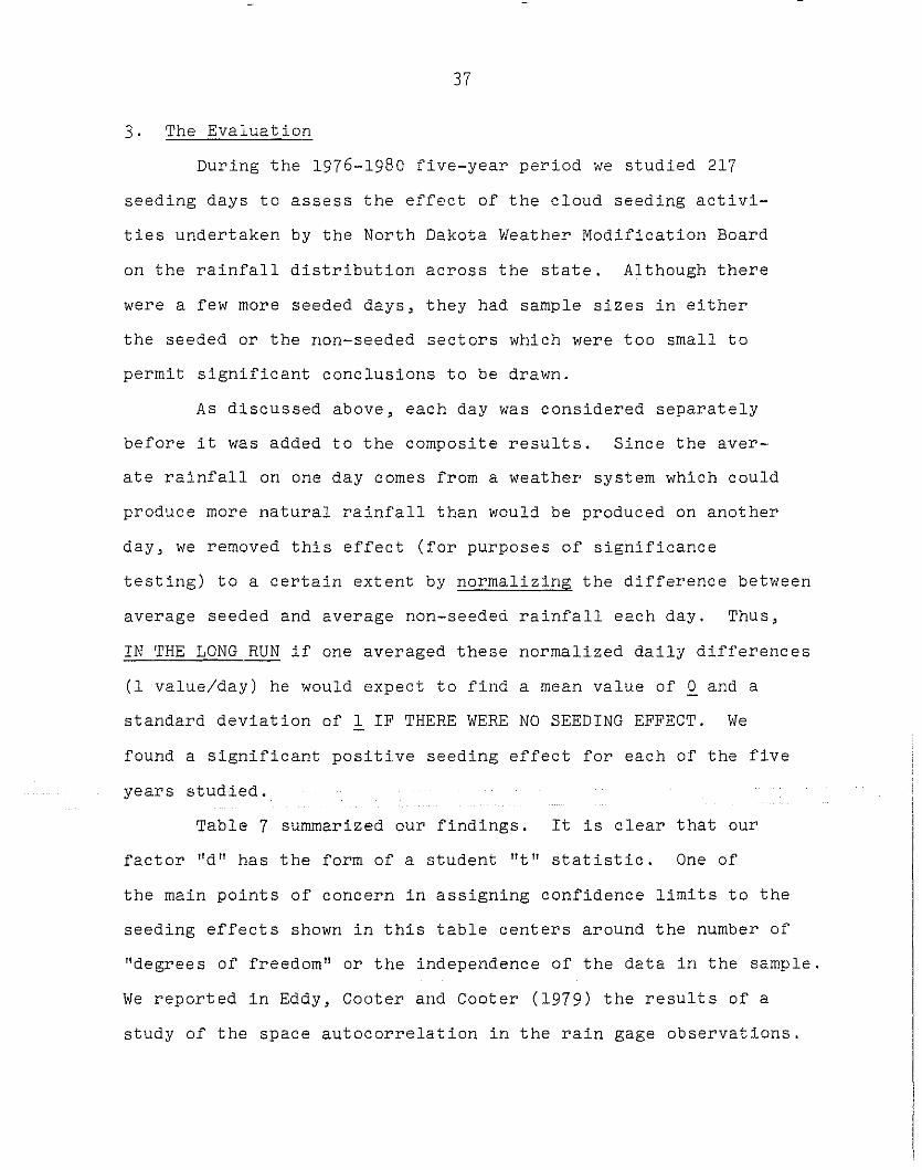
3. The Evaluation

During the 1976-1980 five-year period we studied 217

seeding days to assess the effect of the cloud seeding activi­

ties undertaken by the North Dakota Weather Modification Board

on the rainfall distribution across the state. Although there

were a few more seeded days, they had sample sizes in either

the seeded or the non-seeded sectors which were too small to

permit significant conclusions to be drawn.

As discussed above, each day was considered separately

before it was added to the composite results. Since the aver­

ate rainfall on one day comes from a weather system which could

produce more natural rainfall than would be produced on another

day, we removed this effect (for purposes of significance

testing) to a certain extent by normalizing the difference between

average seeded and average non-seeded rainfall each day. Thus,

IN THE LONG RUN if one averaged these normalized daily differences

(1 value/day) he would expect to find a mean value of 0 and a

standard deviation of 1 IF THERE WERE NO SEEDING EFFECT. We

found a significant positive seeding effect for each of the five

years studied.

Table 7 summarized our findings. It is clear that our

factor "d" has the form of a student nt"~ statistic. One of

the main points of concern in assigning confidence limits to the

seeding effects shown in this table centers around the number of

"degrees of freedom" or the independence of the data in the sample.

We reported in Eddy, Cooter and Cooter (1979) the results of a

study of the space autocorrelation in the rain gage observations.

38

TABLE 7

STATISTICS FROM DAILY VALUES COMPARING SEEDED RAINFALLSTATEWIDE AVERAGE TO NON-SEEDED

RAINFALL STATEWIDE AVERAGE

Xl X2 X3X4 X

5X6 X7

X8

1976 70 54 1.10 .14 6 7 .65 .43

1977 53 43 .85 .15 9 9 .50 .33

1978 47 36 1.13 .17 8 5 .67 .44

1979 63 42 1. 09 .15 8 6 .64 .42

1980 63 42 .95 .15 12 7 .56 .37

5-YEARS 296 217 1. 02 .07 43 34 .60 .39

Xl = Total number seeded days.

X2 = Number seeded days with over 7 non-zero rain reports ineach of seeded and non-seeded areas.

X3

= d = (R -R )/o(R -R ).s ns s nsX4 = Standard deviation of d = 1/(X

2)1/2.

X5

= Number of negative d values "observed" .

X6 = Number negative d values "expected" ifd 'U N(O,l).

X7

= d/1. 69 (adjusted for space autocorrelation).

X8 = X7/1.52 (adjusted now for both time and space autocorrelation).

39

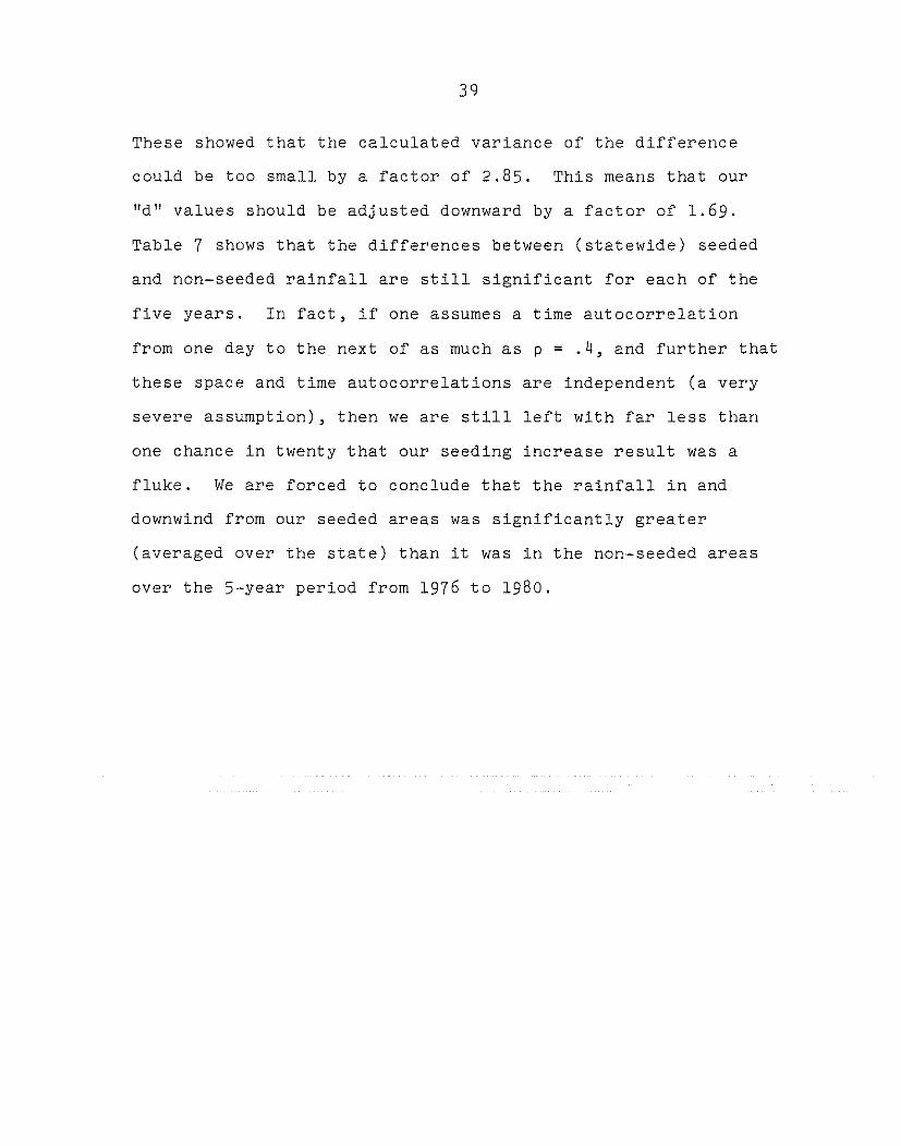
These showed that the calculated variance of the difference

could be too small by a factor of 2.85. This means that our

I'd l l values should be adjusted downward by a factor of 1.69.

Table 7 shows that the differences between (statewide) seeded

and non-seeded rainfall are still significant for each of the

five years. In fact, if one assumes a time autocorrelation

from one day to the next of as much as p = .4, and further that

these space and time autocorrelations are independent (a very

severe assumption), then we are still left with far less than

one chance in twenty that our seeding increase result was a

fluke. We are forced to conclude that the rainfall in and

downwind from our seeded areas was significantly greater

(averaged over the state) than it was in the non-seeded areas

over the 5-year period from 1976 to 1980.

40

4. The Search For Treatments And Covariates

As was discussed in section B above, this is a problem

which looks to several meteorological subdisciplines for a

solution. We have looked at time trends in the climate and

space trends across the state in the daily weather. These were

discussed by Eddy, Cooter and Cooter (1979). The differences

in the cloud physics of the rain processes among air mass

thunderstorms, squall lines, warm frontal rain and cold lows

still need to be quantified. Although this should also be done

from a synoptic climatology point of view, the method we have

chosen to use is an analysis of the thermodynamic and kinematic

structure of the ambient atmosphere over North Dakota during a

particular day, performed on the Bismarck rawinsonde (R/S).

We use a set of computer algorithms developed by Hirsch (1971)

of the South Dakota School of Mines and Technology and

expanded by Dave Matthews of the Bureau of Reclamation. The

Great Plains Cloud Model (GPCM) is a I-dimensional algorithm

which estimates convective clouds which should develop in a given

environment (R/S) provided a trigger mechanism is available.

The surface temperature rise required to set off the instability

is estimated and the consequent natural cloud growth is "predicted".

Further: a modified cloud growth is also "predicted" assuming the

introduction of a specified amount of silver iodide in a speci-

fied manner with a postulated cloud physics process.

41

It is the use of sets of GPCM output for purposes of

stratifying our seeded rainfall increases (or decreases) and for

purposes of looking for covariates upon which we report here.

Tables 8711 show the selection of variables from which we can

choose for our purpose.

Table 12 lists a small sample of eleven ways in which

we have classified each of our 5 years (1976-1980) of data.

Firstly we will define the terms found in that table.

CTT = natural cloud top temperature (Table 10).

CBT = cloud base temperature (Table 8).

TIME = the time it would take a parcel of air to risefrom the base to the top of a natural cloud.This has been estimated using the cloud thickness,the maximum vertical velocity given by the GPCMmodel and a parabolic shape to the verticalvelocity profile (Table 10).

mean rain over all gages lying inareas of the state on a given day500-600 gage special network).

the non-seeded(from NDWMB

= mean rain over all gages in a target area or any­where downwind on a given day (from NDWMB 500-600gage special network).

d = a normalized value of (Rs R ) (Equation 1, p. 48).ns

H = the increase in cloud depth because of silver iodideseeding as predicted by the GPCM (Table 10).

= the maximum updraft speed predicted for thenatural cloud (Table 10).

DIR5 00

= 500 mb wind direction (Table 11).

R 11 = State mean rainfall for a day (from the NDWMBa 500-600 gage special network).

• 42

The mixing depth used in computing theconvective condensation level (CCL) in mb

Cloud base height (km)

Cloud base temperature toe)

Surface convective temperature (OC)

Surface temperature rise required to reachconvective temperature (OC)

Sub-cloud mixing ratio (g/kg)

Environmental mixing ratio; SFC-200 mb (g/kg)

Height of lowest inversion (m)

Mean lapse rate (OC/IOO meters)0-50, 0-100, 100-150, 150-200, 400-500,500-600 millibars above surface

Mean mixing ratio (g/kg); same levels as forXLAPS

Numeric code to

If IABORT = 0If IABORT = 1

If IlI-BORT = 2

If IABORT = 999

indicate if cloud growth

growth was possibleexcessive heating was required toreach convective temperature andgrowth was deemed impossible.the rawinsonde data did not extendto the 200 mb level and the modelwas unable to determine growth.the sounding data were not available.

Table 8: GPCM Output Variables.

• 43

THE WIND SHEARS BELOH ARE FOR NINE ATf10SPHERIC SL!\BS:0-50JO-IOOJ IOO-ISOJ ISO-200J 400-S00J SOO-600J 300-500J

300-700 AND 300-800 MB ABOVE GROUND LEVEL

U Component shear (meters per second)

V Component shear (meters per second)

Directional shear (degrees)

U Component shear (per second)

V Component shear (per second)

T Component shear (per second)

Table 9: GPCM (Analyzer) OutputVariables.

• 44

THE NEXT SIX TAPE RECORDS CONTAIN DAT/l, FORNATURAL AND MODIFIED CLOUDS \'lITH

VAR.IOUS UPDRAFT RADI I

RADIUS (1) = 0.5 kmRADIUS (2) = 1.0 kmRADIUS (3) = 1.5 kmRADIUS (4) = 2.0 kmRADIUS (5) = 3.0 kmRADIUS (6) = 10.0 km

Model cloud radius (km)

Cloud top height (km)Note: For these and the following variables,

J = 1 indicates the natural cloud,J = 2 indicates the modified cloud.

Speed of maximum cloud updraft (m/sec)

Height of maximum updraft (km)

Temperature at the maximum updraft height (OC)

Maximum reflectivity (dB)

Height of the maximum reflectivity (km)

Efficiency of precipitation (%)

Efficiency of condensation (%)

Predicted rainfall (inches)

Natural cloud depth (km)

Modified cloud depth (km)

Cloud top temperature (OC)

Total QC COLD (g/kg)

Total QH COLD (g/kg)

Table 10; GPCM Output Variab~es.

• 45

THE tlEXT SIX RECORDS CONTAIN DAn FOR THEVARIOUS r1ANDATORY PRESSURE LEVELS:200, 300, 400, 500, 700 AND 850 MB

LEVELS, IN THAT ORDER

Pressure in millibars

Height of pressure surface in meters

Temperature at the pressure level (OC)

Dew point depression (Oe)

Relative humidity (%)

Potential temperature (K)

Equivalent potential temperature (K)

Wet-bulb temperature (K)

Saturation wet-bulb temperature (K)

Wind direction (degrees)

Wind speed (meters per second)

Saturation deficit (grams per cubic meter)

Precipitable water SFC - 850 rob

Precipitable water SFe - 700 rob

Precipitable water SFC - 500 rob

Total precipitable water

Height of the ooe isotherm (meters)

Height of the -5°C isotherm (meters)

Height of the -10°C isotherm (meters)

Height of the -15°C isotherm (meters)

Mean mixing ratio of the lowest 100 mb (g/kg)

Lifted index - 100 rob adiabatic

Lifted index - 50 mb layer mean values

Total totals index

George's K-index

Severe weather threat (SWEAT) index

Table 111 GPCM (Analyzer) Output Variables.

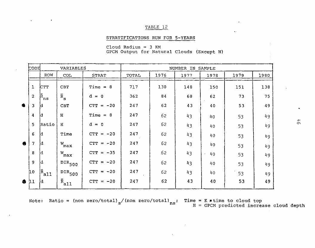
TABLE 12

STRATIFICATIONS RUN FOR 5-YEARS

Cloud Radius = 3 KMGPCM Output for Natural Clouds (Except H)

•

•

•

::ODE VARIABLES NUMBER IN SAMPLE

ROW COL STRAT TOTAL 1976 1977 1978 1979 1980

1 :TT CBT Time = 8 717 130 148 150 151 138

2 Rns Rs d = 0 362 84 68 62 73 I 75

1I3 d CBT CTT = -20 247 62 43 40 53 49I

Time = 8I

4 d H I 247 62 I 43 40 53 49

5 Ratio H I d = 0 247 62 43 40 53 49

6 d Time CTT = -20 247 62 43 40 53 49

7 d W CTT = -20 247 62 43 I 40 53 49max

8 d W CTT = -35 247 62 43 40 53 49I 9

max

d DIR500 CTT = -20 247 62 43 40 53 49

flO RaIl DIR50 0

CTT = -20 247 I 62 43 40,

53 49

fll d RaIl CTT == -20 247 62 43 40I

53 49

•

.c­0"\

Note: Ratio = (non zero/total) /(non zero/total)s ns Time =H =

K "time to cloud topGPCM predicted increase cloud depth

47

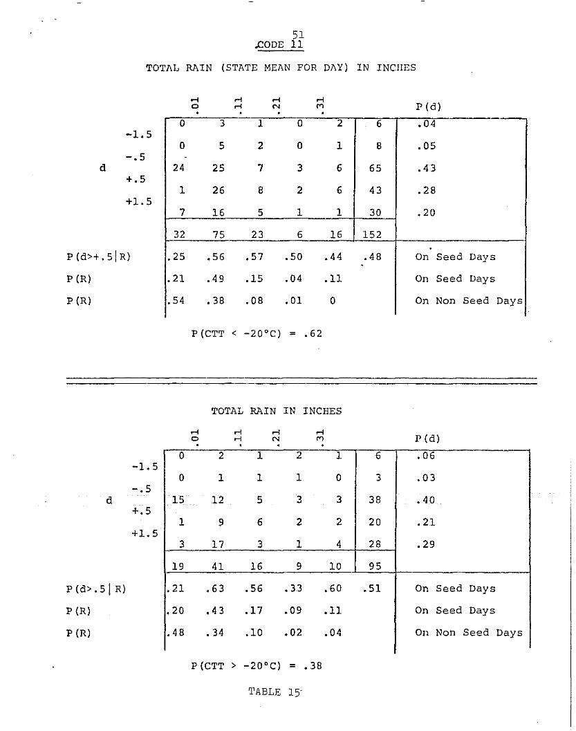
Next we turn our attention to Table 12, codes 3, 7,

and 11. The 5-year composite results of these tabulations are

shown in Tables 13, 14, and 15. These tables all make use of

the GPCM analyses of 5 years of daily 1200z RIS data at Bismarck

during the seeding period each year. (We use April I-Sept. 30);

however, when ~ is used then only seeded days are considered.s

We will describe our system by using code 3 (Table 13)

as an example. The page contains two main tables and the

numbers within each are counts of days in that particular

"slott'. The total count in Table 13 = 247 (152 + 95); this

means that our data set consiste~ of 247 days when we found

values for Rs ' Rn s ' CBT and CTT during the 5-year period.

These 247 days are split into 152 days when the (GPCM predicted

natural) CTT was less than -20°C and 95 days when the (GPCM

predicted natural) CTT was warmer than or equal to -20°C (see

Table 12, column 4, row (code) 3.

In each of the two tables the days are split (columns)

into five CBT categories as shown. Also in each of the two

tables the columns are split (rows) into five normalized-rainfall-

increments (~-~ IoCR" ..~ )).s ns s ns

The sixth column and the sixth

row are sums of the tabular row values and column values

respectively. Estimated conditional and simple probabilities

are also shown.

RS - RNS( 2 2)J./2NsSs + NNSSNS .

WHERE S2 = nN

L1=1

- 2(R

I- R)

AND

RSI = A RAIN REPORT IN A SEEDED SECTOR

RNSI = A RAIN REPORT IN THE NON-SEEDED AREA

A RAIN REPORT = THE·24-HOUR RAINFALL BETWEEN0700 LST AND 0700 LST

EQUATION 1

•

-'="D:>

-1.5

-.5d

+.5

+1.5

P(d~+.5ICBT)

P(CBT)

P(CBT)

,?ODE 349

CLOUD BASE TEMPERATURE °C

InIn In • LI). • N •f'- N r- P (d)I I + +

0 0 0 3 3 6 .04.,

0 . 0 0 2 6 8 .05

1 1 7 19 37 65 .43

0 0 4 12 27 43 .28

0 0 3 12 15 30 .20

1 1 14 48 88 152

0 0 .50 .50 .48 .48 On Seed Days

.01 .01 .09 .32 .58 On Seed Days

On Non Seed Days

P(CTT < -20°C) = .62

CLOUD BASE TE~PEP~TURE °C

In.r­I

LI1•

NI

LI1.N+

.r­+ P (d)

-1. 5

-.5d

+.5

+1.5

P(d>+.5!CBT)

P (CBT)

P(CBT)

0 0 0 1 5 6 .06

0 0 0 0 3 3 .03

0 1 3 17 17 38 .40

0 0 3 5 12 20 .21

0 1 2 13 12 28 .29

0 2 8 36 49 95

- .50 .63 .50 .49 .51 On Seed Days

0 .02 .08 .38 .52 On Seed Days

On Non Seed Days

P(CTT > -20) = .38

TABLE 13

CODE 7 5G

MAX VERT HOTION IN MiS

l' (d)

-1.5

-.5d

+.5

+1.5

P (d>+. 51 Hmax

)

P (Hma)

P (Wma x )

-1.5

-.5d

+.5

+1.5

P(d>+.5IH)m

0 0 1 1 4 6 .04

0 0 0 0 8 8 .05.

0 1 4 10 50 65 .43

0 0 1 4 38 43 .28

0 0 1 6 23 30 .20

0 1 7 21 123 152

_. 0 .29 .48 .50 .48 On Seed Days

0 .01 .05 .14 .81 On Seed Days

On Non Seed Days

P(CTT < -20°C) = .62

MAX VERT MOTION IN MIS

P (d)

3" 3 0 0 0 6 .06

1 1 1 0 0 3 .03

7 16 10 2 3 38 .40

3 4 6 6 1 20 .21

7 12 7 2 0 28 .29

21 36 24 10 4 95

.48 .44 .54 .8 .25 .51 On Seed Days

.22 .38 .25 .11 .04 On Seed Days

On Non Seed Days

P(CTT > -20°C) = .38

TA13LE 14

51.cODE 11

TOTl\L RAIN (STATE MEl\N FOR Dl\Y) IN INCHES

.-i .-i .-i .-i0 .-i N M• . . P (d)

-1.5

-.5d

+.5

+1.5

P (d>+. 51 R)

P (R)

P (R)

0 3 1 0 2 6 .04

0 5 2 0 1 8 .05.

24 25 7 3 6 65 .43

1 26 8 2 6 43 .28

7 16 5 1 1 30 .20

32 75 23 6 16 152

.25 .56 .57 .50 .44 .48 On Seed Days-

.21 .49 .15 .04 .11 On Seed Days

.54 .38 .08 .01 0 On Non Seed Days

P(CTT < -20°C) = .62

TOTAL RAIN IN INCHES

.-io. .-i

.-i. .-iN. P (d)

-1.5

-.5d

+.5

+1.5

P(d>.5! R)

P (R)

P (R)

0 2 1 2 1 6 .06

0 1 1 1 0 3 .03

15 12 5 3 3 38 .40

1 9 6 2 2 20 .21

3 17 3 1 4 28 .29

19 41 16 9 10 95. -.21 .63 .56 .33 .60 .51 On Seed Days

.20 .43 .17 .09 .11 On Seed Days

.48 .34 .10 .02 .04 On Non Seed Days

P(CTT > -20°C) = .38

TABLE 15-

52

Tentative inferences

Table 13: d, CBT, CTT:

1) rainfall increases associated with seeding pre­dominate rainfall decreases no matter what thecloud top temperature and no matter what thecloud base temperature,

2) there are twice as many cold cloud tops aswarm cloud tops in this data set,

and3) by far the most clouds in this North Dakota

data set have base temperatures warmer than+2.5°C.

Table 14: d, W , CTT; additional inferences:max1) warm cloud tops are associated with slow

maximum vertical motions and cold cloud topswith fast vertical motions,

and2) in the case of the warm cloud tops, the posi­

tive d values (Eqn. 1) seem not to be associatedwith any particular vertical motion, althoughthere is a tendency to peak around 11-12 m/s;while in the case of the cold cloud tops, thepositive d values (seeding rainfall increase)tend to cluster around the fast updrafts.COULD THE SEEDING OF LARGE (TALL=COLD TOP)CLOUDS TO REDUCE HAIL, ALSO BE INCREASING RAIN?

Table 15.: d, Ra ll , CTT; additional inferences:

a) most of the daily mean rainfall for this NorthDakota data set is less than 1/4 inch with thepeak (mode) around 1/10 inch. This seems to beindependent of the CTT,

andb) with warm cloud tops, the seeding is more likely

to produce rainfall increases in synoptic situa­tions delivering less than .2 inches (statewideaverage); whereas, for cold cloud tops, therainfall increases are likely to occur with aslightly higher statewide average rainfall.

53

In the above analyses, the R/S observation used was

1200z on the same date as the rain report. This means that the

upper air sounding was timed to occur at the end of the 24-hour

on which the rain fell, as indeed was the rain measurement

itself. The following tables present the analysis results for

1980 code 7 (d, Wma x' CTT) to provide a comparison between

the 1200z R/S as used and the sOl\l1ding 12 hours earlier at OOOOz.

This earlier sounding would haVe been tak~n near suppertime dur­

ing the time of the maximum (on the average) convective activi­

ties which produced the measured rainfall.

Although the sample size in Table 16 is small, the con­

clusions drawn as regards the seeding rainfall increases as a

function of maximum (natural) vertical motion and (natural) cloud

top temperature remain unchanged. The main consequence of this

change in R/S timing is to lose part of our data set if we choose

the afternoon sounding.

The above is only a sample of the planned analyses.

Future stratifications will be guided to a major extent by the

Todd-Howell hypotheses concerning the cloud physics of pre­

cipitation enhancement.

One very important aspect of the above results must be

underscored: the GPCM itself acts as a stratifier of weather

types. There is a considerable amount of rainfall which is not

of the convective type and which would show up in the model out­

put as IABORT = 0 or 1. Thus the day involved would not show

W MiS Wma x MiSmax RIS at 0000 GMT 1980

rl tr\(Y) t-- rl rl rl tr\

I(Y) t-- rl rl

0 0 0 0 1 0 0 0 0 0-1. 5 I -1. 5

0 0 0 0 1 I 0 0 0 0 0-.5 -.5

d 0 0 1 3 2 d I 0 2 3 0 0•+.5 +.5

0 0 1 0 4 I 2 0 0 0 0+1. 5 I +1. 5

0 0 0 0 2 I 1 4 0 0 0

CTT L.T. -20°C CTT G.E. -20°C

\J1.<0-

W MiS Wma x MiSmax

R/S at 1200 GMT 1980rl tr\ rl tr\

(Y) t-- rl rl (Y) t-- rl rl

0 0 0 1 1 I 2 0 0 0 0-1. 5 I -1.5

0 0 0 0 1 I 1 0 0 0 0-.5 -.5

d 0 0 1 3 12 d I 2 3 2 0 1+.5 +.5

0 0 0 0 9 I 0 0 0 1 0+1.5 I +1.5

0 0 1 1 3 I 2 2 0 0 0

CTT L.T. -20°C CTT G.E. -20°C

Table 16: Code 7 Cd, Wma x' CTT).

55

up in the above analysis. This "stratification by default"

must be done in a more positive sense------possibly by using

variables such as positive vorticity advection.

Although there is still a good way to go before the

clusters and covariates can be specified objectively, the job

can be done and the results will be valuable.

56

D. IMPACT

This section of our report is presented in two segments.

Segment 1 discusses an approach to the analysis of agricultural

drought in North Dakota which was developed by the author and

Ellen Cooter in 1978 and the relevant portions of that report

are presented in the following pages. We have considered spring

wheat for illustrative purposes and both precipitation and

temperature effects are integrated through the use of a simple

hydrologic accounting system. The purpose is to illustrate the

manner in which the agricultral community across the state can

expect those climate parameters which most affect their industry

to vary naturally over many years. Figure 22 shows that the

state is vulnerable to both short-term and long-term drought

and it is for this reason that we have begun to define those

climate variables responsible in order eventually to assess the

value of weather modification in reducing the impact of these

naturally occurring disasters.

Segment 2 deals with the economic impact on the state of

rainfall enhancement over the 1976-1980 period. Dr. Cooter has

used 14 crops for his analysis and drawn on several sources of

expertise in the State of North Dakota for his information on

local agricultural economics.

57

Areas vulnerable to drought

SOURCE: United States Department at the Interior, Geological Survey, 1970The National atlas of the United States of America"

nGURE 22

Humid Cllmalo wl1hWAlorSUlphj!o, ovonOuting PoriOd! 0' Los,lhOl>AveraC/1l Ploclpllll<lion

58

1. Drought In North Dakota

Time series of daily values of precipitation, maximum

temperature and minimum temperature were obtained from the

National Climate Center for 55 National Weather Service

stations across North Dakota. Data from all stations in each

of the nine flimate Qivisions were averaged over a week in

the case of temperatures, and daily averages were summed for

a week in the case of precipitation. Figures 23 and 24 give

examples of short portions of these weekly by CD average

values for mean temperature and for precipitation taken from

CD9. Drought characteristics must be deduced from some

combination of pairs of such superficially incredibly dis­

similar series.

As another drought indicator, we obtained Hard Red

Spring (HRS) yield data for each year between 1929 and 1975

for each of our 9 Climate Divisions in North Dakota.

The decision was made to investigate three methods of

combining the temperature and precipitation data for the pur­

pose of assessing drought conditions. All three have been

developed by W. C. Palmer and were reported by him in 1965

and 1968.

Soil moisture (SM) and evapotranspiration (ET) come

from using Palmer's 1965 system for integrating the basic

variables on a weekly basis instead of the monthly interval

he chose for his own studies. The crop moisture index (CMI)

basically follows the procedure used currently to produce the

charts published by the USDA/NOAA weekly Crop and Weather

Bulletin.

Fi~ure 23: Weekly North Dakota CD 9 (SE) Temperature Detail (1934r1942).Tick MarkaBegin Year.

V1

'"

t-

90[-----r-------------~I i

60

o

~

JIoo'-'

1'.; 30 .~ !J.ilE-!

193 193YEAR

1940 1942

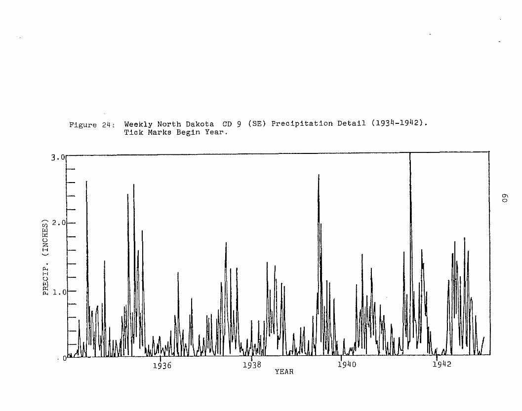
Figure 24: Weekly North Dakota CD 9 (SE) Precipitation Detail (1934-1942).Tick Marks Begin Year.

3. 0'1 - - - - - - - - - - - - - - - - - - - - - - - ....-- - - - -I I

-;;)2.0~::r:o:z:H

0\o

~

p,Ho~p.,

t-

ollle y ! I IIUUVYh d vt/v"iVlIBIIU IO'I-V·oj· 1/U.-.III 1\1lJk1'~Oll lr lin IYV I "WIll] 'I\~ N! I 'W I

, I I

YEAR

61

a. Soil Moisture

Soil moisture (SM) for this study was calculated using

a hydrologic accounting system similar to the one reported by

Palmer (1965). Soil moisture is previous storage plus pre­

cipitation (P) minus evapotranspiration (ET) up to a set

maximum (Table 17). Excess P is runoff. A surface layer can

supply up to one inch to ET, but only a fraction of demand

beyond that will be supplied by the underlying layer. Evapo-

transpiration is that part of a potential evapotranspiration

(PET) which is satisfied. Thornthwaite (1968) gives:

PETi = CC1.6(5.555 6(Ti-3 2)/B)A)HOURS/12)/2.5 4/C30/7)

where = weekly/CD average temperature in of.CPET=O when T < 32),

Ti = long term weekly/CD average temperature of,

HOURS = number of daylight hours,

7/30 = transformation from monthly values used byThornthwaite to weekly values used in thisstudy,

B = heat index computed from long term record

= Cl/4)52L

i=l«T._32)/5)1.5 1 4

lwhere Ti is set = 32

if it is climatologi­

cally < 32,

A = .49239 + .01792B - .0000771B 2 + .000000675B'.

At this point it should be mentioned that our present use

of soil moisture is as a predictor variable in a linear regression

62

equation and hence it is the deviations of this variable

about its linear trend (essentially its long-term mean) which

is important. Thus, small differences between the calculated

PET long-term mean and the "true" value of its long-term mean

will make no significant difference to our end results. The

main consequence of such a difference will show up as a small

decrease in the time constant of soil water depletion, but will

make very little difference in the ability of our procedure to

detect major drought signatures.

The average soil available water capacity (AWC) of each

crop district has been obtained by Palmer and is in current use

by the National Weather Service. We obtained these values from

Lyle Denny of the National Weather Service as tabulated below.

CRD NORTH DAKOTA

1 6

2 7

3 7

4 8

5 8

6 8

7 8

8 8

9 8

Table 17: Available Water Capacity (AWC)Values In Inches.

63

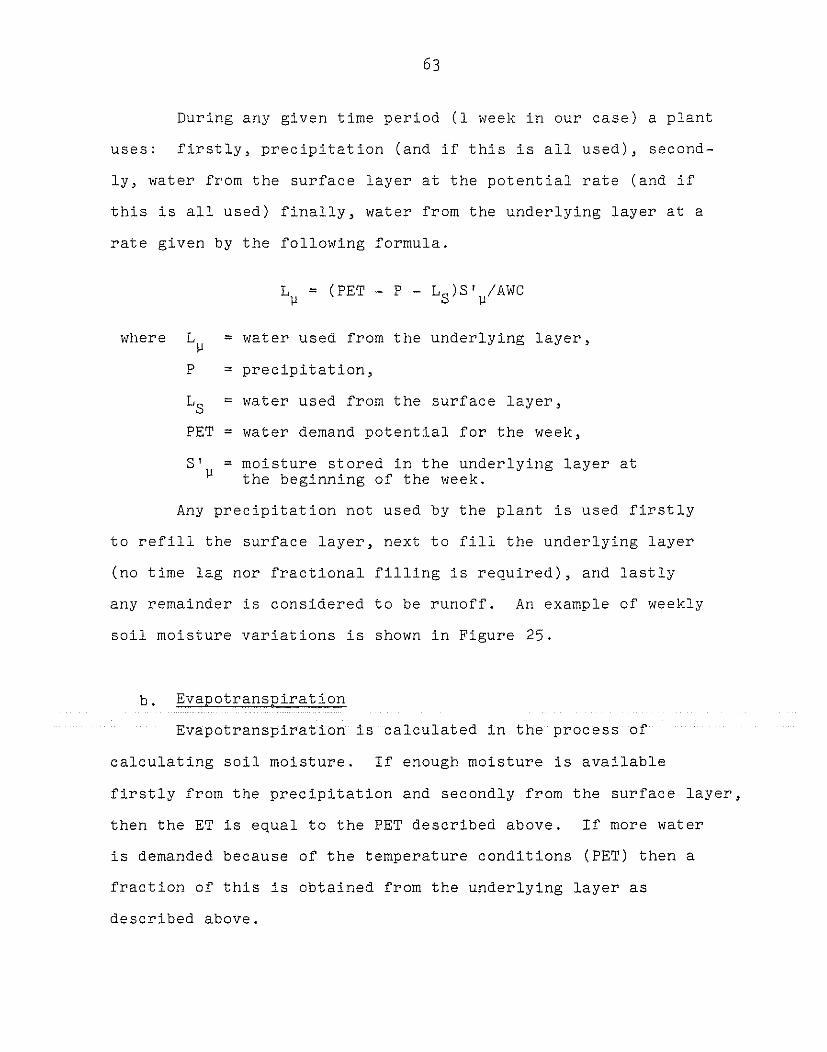
During any given time period (1 week in our case) a plant

uses: firstly, precipitation (and if this is all used), second-

ly, water from the surface layer at the potential rate (and if

this is all used) finally, water from the underlying layer at a

rate given by the following formula.

where L = water used from the underlying layer,jJ

P = precipitation,

LS = water used from the surface layer,

PET = water demand potential for the week,

S' u = moisture stored in the underlying layer atthe beginning of the week.

Any precipitation not used by the plant is used firstly

to refill the surface layer, next to fill the underlying layer

(no time lag nor fractional filling is required), and lastly

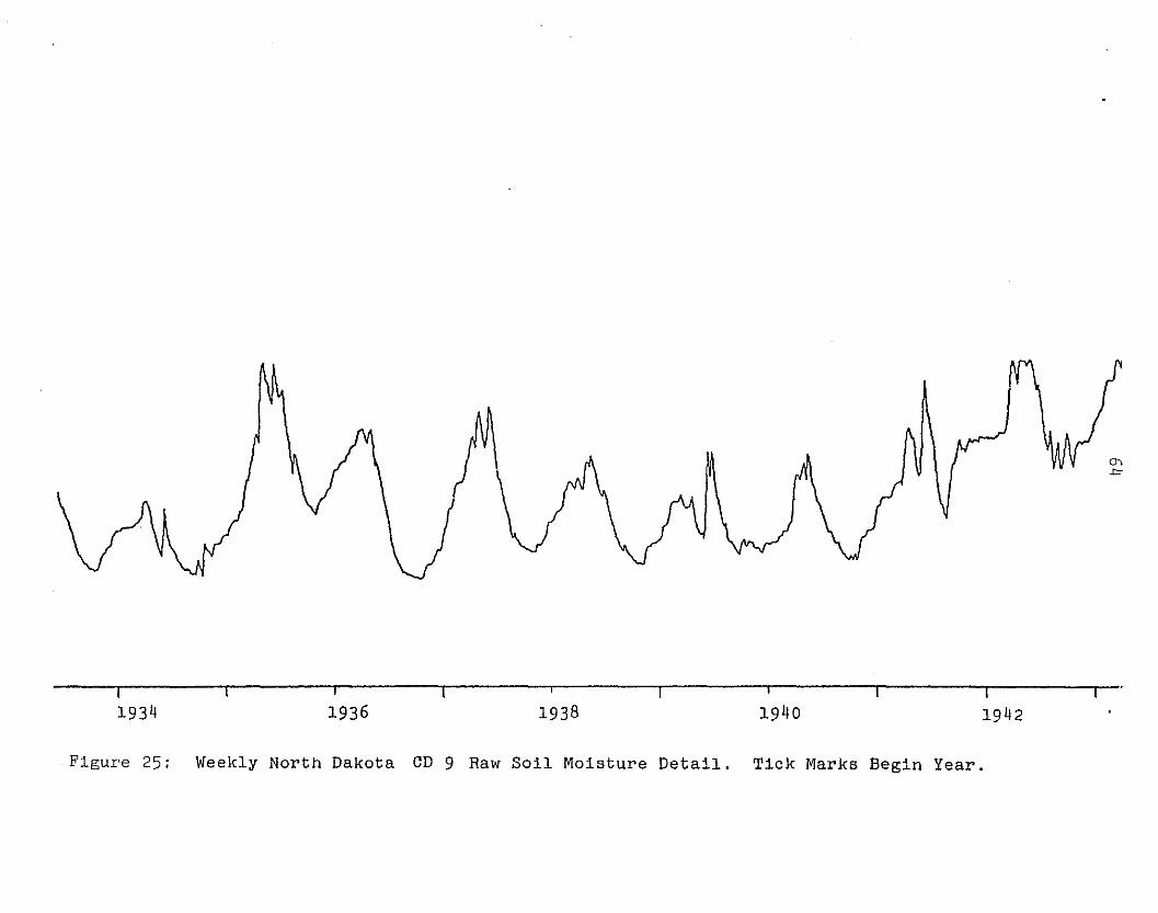
any remainder is considered to be runoff. An example of weekly

soil moisture variations is shown in Figure 25.

b. Evapotranspiration

Evapotranspiration is calculated in the process of

calculating soil moisture. If enough moisture is available

firstly from the precipitation and secondly from the surface layer,

then the ET is equal to the PET described above. If more water

is demanded because of the temperature conditions (PET) then a

fraction of this is obtained from the underlying layer as

described above.

I I r~--~ I I ~--~-I u ~~~-- I U -----1 I I

1934 1936 1938 1940 1942

Figure 25; Weekly North Dakota CD 9 Raw Soil Moisture Detail. Tick Marks Begin Year.

65

It is clear that ET can vary directly with the precipi-

tat ion (under fairly peculiar temperature fluctuations) while

the 3M remains constant. A nine-year portion taken from a

typical weekly ET series is given in Figure 26.

c. Crop Moisture Index

The CMI reported by Palmer (1968) combines soil moisture,

evapotranspiration, recharge and runoff. The algorithm ~ use

follows: where i designates a given week:

= 0 if 3M = 0

+where

= -1 when i=l

= 0 when i=l

and H = Gi

_1 if 0 < G < .5i",l

= .5 if .5 < Gi

_l

< 1.0

= .5Gi_

lif 1 < G

i_

l

= 0 if

+The formula advocated by Palmer accentuates ET slightly more; i.e.,Y - 6 8[ -1/2 1/21 - . 7 Y1-l + 1. ET1 a - PET1 a ].

u L '--~

I

l u

0\0\

J I I - ----T ~- ~ ~ I

1934 1936 1938II l ----I ~ ~-·~··I

1940 1942

Figure 26: Weekly North Dnkotn CD 9 (BE) Evapotrnnapiratlon Detail (1934-1~42),Tick Marks Begin Year.

PET i =N

(liN) Lj=l

67

N = number of years in data series

AWC = available water capacity (see Table 17).

Short examples of weekly CMI are given in Figures 27 and 28

to illustrate the contrast between the two methods of calculating

crop moisture index. Our method accentuates dry periods slightly.

d. Growing Season Soil Moisture and Evapotranspiration

In order to obtain reasonable representative values for the

total amount of SM and ET influencing the growing season, weekly

values of these variables were summed each year for weeks 21-28

inclusive.

e. Modelling the Data

The object of modelling our derived variable series here

is to find an attribute which can be depended upon to indicate

the occurrence of drought as a sporadically recurring phenom-

enon. If we are planning to look for prolonged excursions of

the data from its mean value, we must first be sure that the

mean value is not changing significantly with time. We did not

find statistically significant linear trends in soil moisture,

evapotranspiration nor crop moisture index in the weekly value

time series.

The next step was to examine the distribution of the weekly

values about the 63-year mean for the series.

Figure 27: Weekly North Dakota CD 1 (NW) Crop Moisture Index Detail (1934-1942)(after Palmer). Tick marks begin year.

+2.0 I i

(/JiLl::r.:'-'zH

+1.0

o

-1.0 I

0-.co

I\ I

1942• •

1940III

~- 19381936-2.0 I « I

Figure 28: Weekly North Dakota CD 1 (NW) Crop Moisture Index Detail (193~~19~2)

(this study). Tick marks begin year.

+2.0 I I

[J)

[tioZH

193I J

1938 19~O 1942

YEAR

o-,\D

70

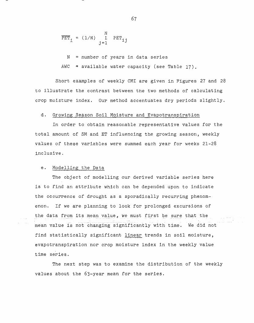
The histograms shown in Figures 29, 30, and 31 contain

a wealth of information about the character of the data. At

this point, attention is drawn to the histogram in each figure

marked RAW. The frequency count in each category has been

standardized to 1000 and plotted as heavy dots against a back-

ground showing a Gaussian distribution. Both the mean value for

the RAW data series is given and the RMS value about this mean.

A measure of the variation of the actual observed data frequencies

(Oi) about the appropriate non-standardized Gaussian value (Ei)

is given labelled X2 , where:

In some cases this value varies as CHISQUARE with 9 degrees

of freedom (x 2 . 01 , 9 ~ 22).

Consider the soil moisture first. The plots for North

Dakota show no terrible non-gaussian deformities, although the X2

values suggest that one may be present.

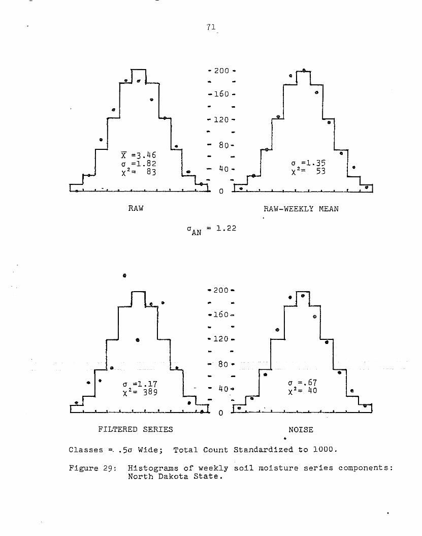
Next we examine the raw evapotranspiration. Figures 26

and 30 show immediately that we will have a problem. Not only

do we have runs of zero values in the winter, but the wintertime

variations are zero and so this type of derived variable is

heteroscedastic or non-stationary with respect to the variance.

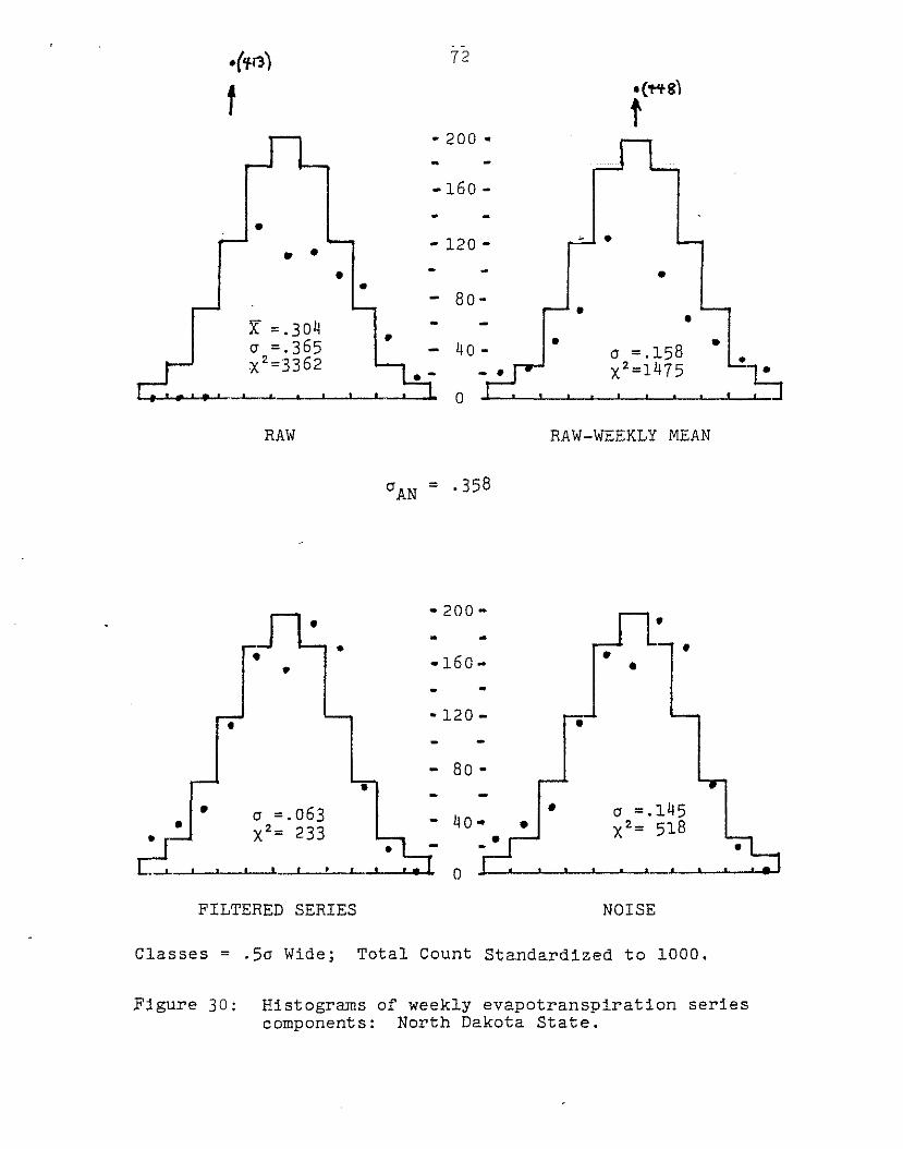
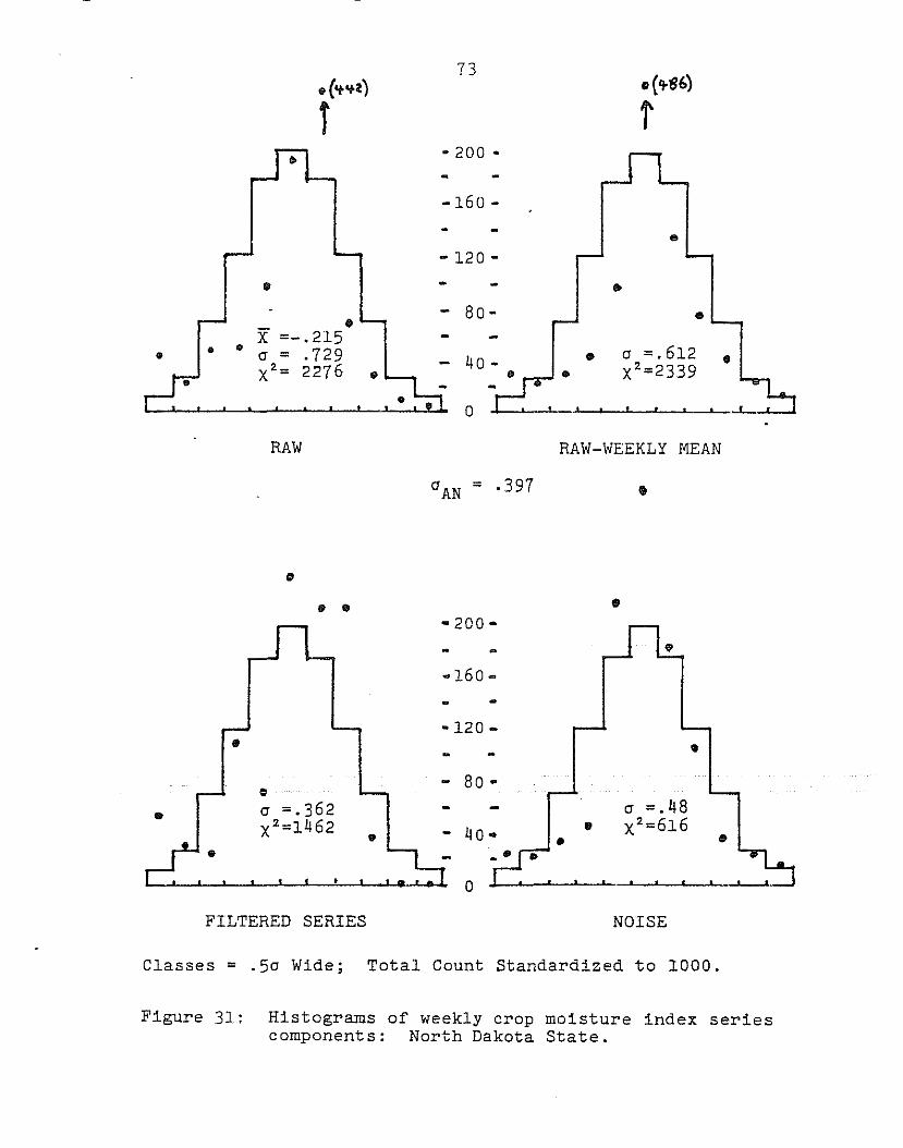
The crop moisture index (CMI) was investigated using the

North Dakota data and the distribution function aspects of the

results are shown in Figure 31.

·200 -

--160 - "

""

- 120- "

"" - 80-

X =3.46 "a =1.82

40 -a =1.35

X2= 83 X2= 53 ••

0

RAW RAW-WEEKLY MEAN

°AN = 1.22

"

"

"

""

"

a

- 200-

" - ..-160-

--120 -

- 80 -

- 40"

•

•.. .

FILTERED SERIES•

NOISE

Classes =.. 50 Wide; Total Count Standardized to 1000.

Figure 29: Histograms of weekly soil moisture series components:North Dakota State.

.('f(;) 72

f • ('1"1-8)

t- 200 -

--160 -

-"- 120- - •

" ""- 80- •

X =.30 11 ••CI =.365 40 - •

CI =.158 "XZ=3362

XZ=1475 •

0

RAW RAW-WEEKLY MEAN

ClAN = .358

- 200-

-•" •• -160 -• •-

-120 - ••

- 80 -•

" =.063 " CI =.1 115CI

" Xz= 233 " Xz= 518•

0

FILTERED SERIES NOISE

Classes = .5a Wide; Total Count Standardized to 1000.

Pigure 30; Histograms of weekly evapotranspiration seriescomponents: North Dakota State.

•

e

a =.612X2 =233 9

•

e

•o

73.('t...~)

T·200 •

-160 -

- 120-

lil

- 80-•X =-.215• • .729• a =

40 -X2 = 2276 •

RAW RAW-WEEKLY MEAN

•

• •- 200"

-160 -

•

lil-120 -

•

•lil

•

o

- 40"

- 80-

•

oa =.362X2 =1 462

••

FILTERED SERIES NOISE

Classes = .5a Wide; Total Count Standardized to 1000.

Figure 31; Histograms of weekly crop moisture index seriescomponents: North Dakota State.

74

Although the statistically most satisfying series to

work with would be the temperature, one of the least satisfying

is the precipitation (see Figure 24, for example) and a drought

deals with a lack of water. We must use some combination of

supply (precipitation) and demand (temperature induced evapo-

transpiration) .

Much of the above problem with skewness in our data

series can be removed by removing an annual cycle of weekly

averages.

We will consider this by analyzing the following model

for the derived data series.

x = u + a + s + S

where X = the "observed" data value (actuallythe average over a week and a CD)

u = the mean

a = an annual cycle component

s = a component we shall call our signatureseri.es

s = noise.

We shall perform our partitioning in such a way that,

cr 2 ~ u 2 + cr 2 + cr 2 + cr 2X ass

The curves derived from the raw data to represent the

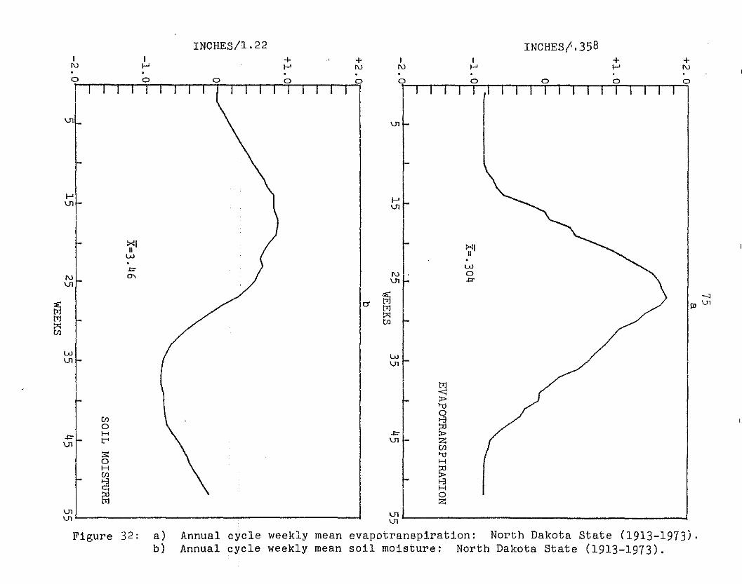
term, a, are shown in Figures 32, and 33, for CMI, ET and SM.

It is interesting that the soil moisture and evapotranspiration

curves are about 3 months out of phase with one another. The 52

o

+ro

--JllJVl

+I-'

oo

INCHES!'.358

o

If-'

><1II

wo

""'"

wVl

ItrJ<:;I>'U0t-3::u

~1-;I>z(j)'1jH

~t-3H0Z,

VIVl

0' .~trJ::>:(j)

Vl

Iro

oo

+I\}

+I-'

oo

INCHES/l. 22II-'.o

(j)oHt-'

:s:oH(j)

~[;l

II\}.o

Vl

wVl

.l="V1

~I I

~tTl

G

Figure 32: a)b)

Annual cycle weekly mean evapDtranspiration: North Dakota state (1913-1973).Annual cycle weekly mean soil moisture: North Dakota State (1913-1973).

+2.0 I I

-1. 0

+1. 0t-ov

'"

--;j

0"\

CROP MOISTURE INDEX-.215

o

."­til

!::JoZH

-2.0 I I J I I I I I ) I I I

5 15 25WEEKS

35 1t5 55

Figure 33: Annual cycle weekly mean crop moisture index:North Dakota State (1915-1971).

77

values for "a" on each of these curves are given by

1 Na j = I Yi j, j = 1, 2, ... 52N i=l

where N = number of years in the data set.

Note that these annual cycles were obtained from normal-

ized data so the numbers along the ordinate must be multiplied

by the standard deviation and then the result added to the mean

to obtain the true scale in inches.

After removing the annual cycle of weekly mean values

from each of the series we were left with data distributed as

shown in the RAW-WEEKLY MEAN histograms shown in the upper

right of Figures 29 - 31 inclusive. The skewness problem has

been reduced, but not eliminated.

At this point we would like to filter our remaining data

components to try to discover slowly varying deviations from

the mean which could be indicators of phenomena such as droughts.

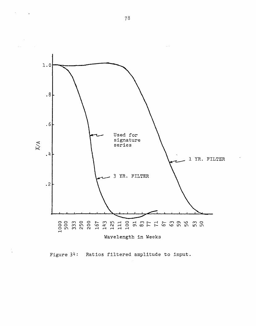
Two low pass filters were tested for this purpose. Figure 34

shows their response functions. These filters were designed

following the procedure of Lanczos (1956). The manner in which

they operate on the time series is shown in Figures 34, 35,

and 36.

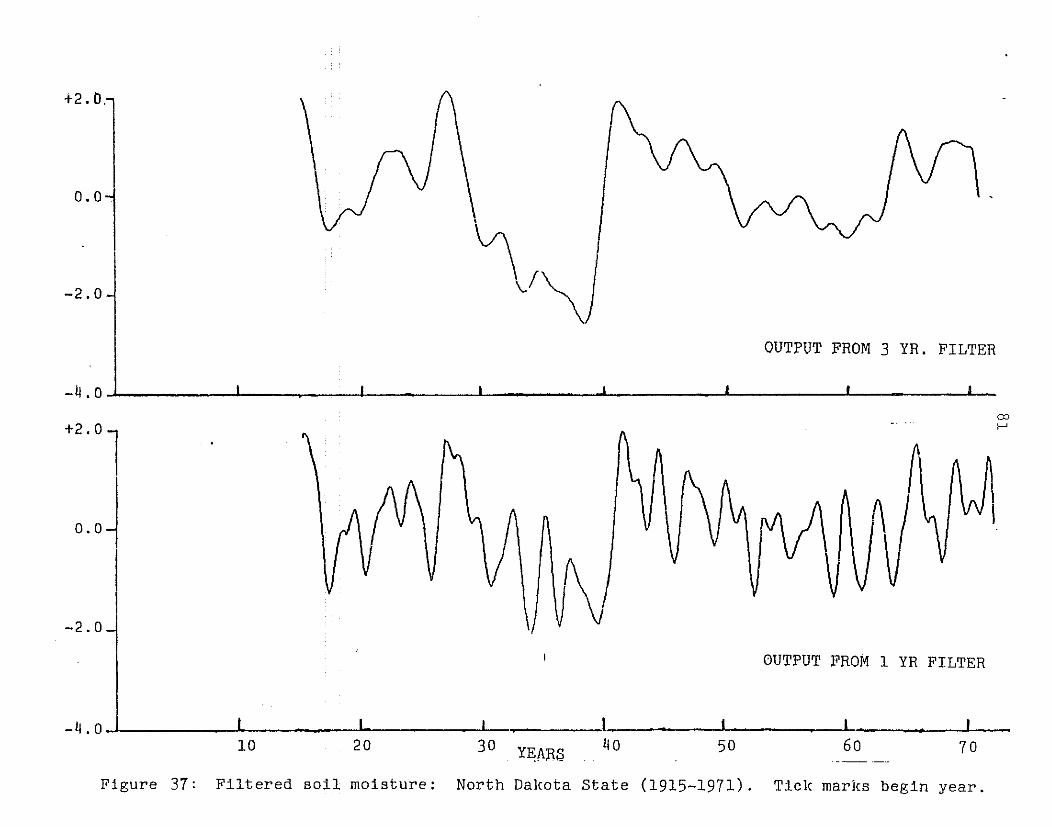
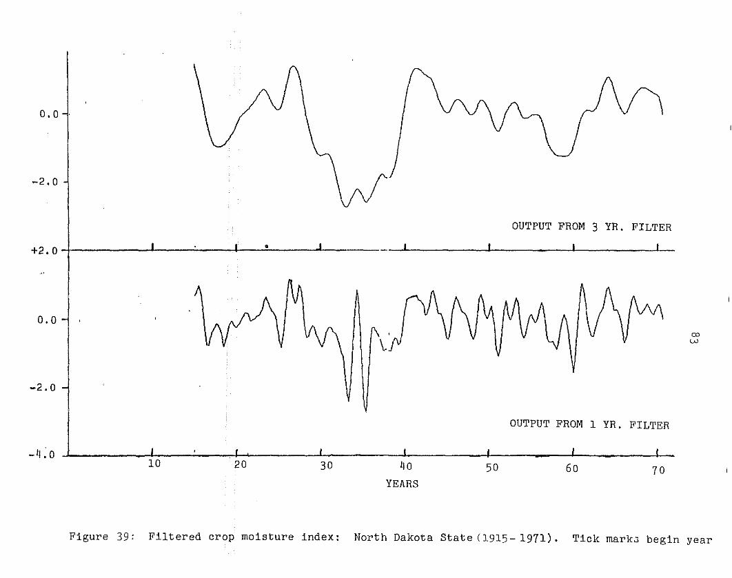
We are now able to show the DROUGHT SIGNATURES which can

be obtained using climatological time series of soil moisture,

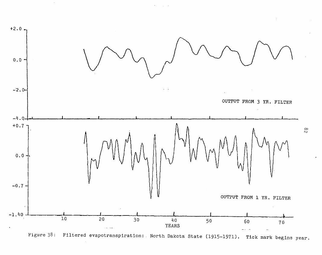
evapotranspiration and crop moisture index. Figures 35, 36, 37, 38

and 39 show that long lasting droughts are shown best using the

3-year filter and short intense droughts are highlighted by the

I-year filter.

78

.4

. 6

1 YR. FILTER

Used forsignatureseries

3 YR. FILTER

.8

.2

1. 01-0:::--------

00 ('r) 00 t-, en l{"\ l"""i 0 M ('Y")t- r-i r:- ('T"'JO\\O (Y)OOO(Y)l{"\O\O~Nl"""iO~Wt-r:-\O\Ol{"\l{"\l{"\l{"\

o Lr\ (Y) N N r-i r-l r-f r1 H.-i

Wavelength in Weeks

Figure 34: Ratios filtered amplitude to input.

.....,\0

i93q I 1936 I --{938 I 19QO I 1~42 I

Figure 35: Weekly plus 3 year filtered N.D. State soil moisture (Raw-weekly) detail (193Q-19Q2).Tick marks begin year.

coa-.

~ I \ ./ "\ -- / \ I :~

.......--:::<::------

.-----.,---- - I" -- --1- I

i93 11 1,936 1938I ·r I --T -- I

19 110 1942YEARS

Figure 36: 1 year filtered plus 3 year filtered ND State soil moisture detail (l934~1942).Tick marks begin year.

~f~0.0 .

+2. O.

-2.0

OUTPUT FROM 3 YR. FILTER

_~ • 0 I I I I I I I I

+2.0

0.0

-2.0 1\AJ\

00f-'

OUTPUT FROM 1 YR FILTER

10 20 30 YEARS

Figure 37: Filtered Boil moisture: North Dakota State (1915-1971). Tick marks begin year.

+2.0 •

0.0 ~

-"2.0

OUT~UT FROM 3 YR. FILTER

OJro

OUTPUT FROM 1 YR. FILTER

O. 0 -;,

_ il. Q..j J I I I I I I I

+0. 7 ~ •

-0.7

10 20 30 ~O

YEARS50 60 70

~igure 38: Filtered evapotranspiration: . North Dakota State (1915-1971). Tick mark begins year.

0.0

-2.0 vVOUTPUT FROM 3 YR. FILTER

L--__~__._L_ ..~~__ L_____ I• ••I I J+2.0 I

0.0

-2.0

CDW

OUTPUT FROM 1 YR. FILTER

10 20 30 ~o

YEARS50 60 70

Figure 39: Filtered crop moisture index: North Dakota State (1915- 1971). Tick markJ begin year

84

Soil Moisture

The longest, driest period found in the state average

of any of the four areas occurred with a 97-week run (SM < -2.5a)

from early June 1938 to mid-April 1940 in North Dakota. In

fact, the rarest event in the entire length of the soil moisture

signature series was a run of 347 weeks with SM < -1.5a from

mid-December 1933 to early August 1940 in this northern wheat

growing state. Figure 40 shows that the consequence of this

on H.R.S. wheat production was to cut the yield to half what

could have been expected had "average" soil moisture conditions

prevailed at the time.

Evapotranspiration

Here, the greatest departure below average was a run

(ET < -2.25a) of 78 weeks from early November 1933 to early May

1935. A run of 217 weeks with ET < -1.5a occurred between

mid-April 1933 and early June 1937.

Crop Moisture Index

The driest period in the CMI signature series was a

50-week run below -2.25a between early September 1933 and late

August 1934. The rarest event of any series of any parameter

occurred with a 357 week run (CMI < -1.5a) from late December

1932 to late October 1939 in the North Dakota state average

signature series of the crop moisture index.

In order to estimate the number of times in a given period

(say 20 years, or 100 years) that the people of North Dakota

could expect a drought of a given severity and duration to occur,

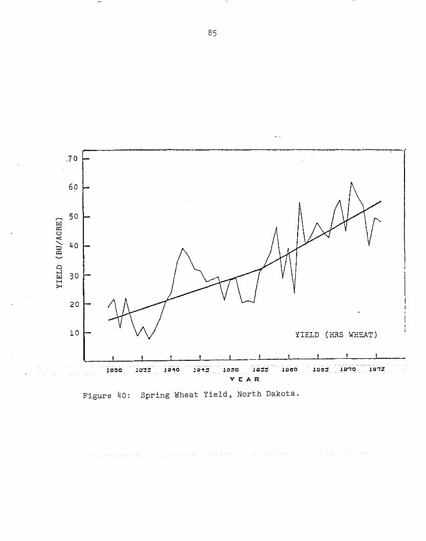
85

Joe:! llnO

YIELD (~~S wrlEAT)

JOBO10:l0 JQ:l:l

Vf:AR

191019::10

,....---------'-------------_._--,.,_ .

10

60

.70

~ 50I::la:;0«:<, 40::>ca~

Cl...:I

30I::lH><

20

Figure 40: Spring Wheat Yield, North Dakota.

86

we simulated the "signature series" stochastic component using

a red noise model. Since the properties of such a model are

known, we were able to hypothesize drought recurrences based

on these simulations.

The long drought of the 1930s showed up with the

expected intensity and coherency. Such a run was found only

two times in thirty simulated 60-year series. Thus the fre-

quency with which North Dakota can expect to endure a drought

like that of the 1930s is about twice in thirty 60-year time

spans. This would also happen about once in thirty 30-year

time spans. This comes to about once in 900 years [provided,

of course, the underlying basic climatology doesn't change

over such a period].

The analysis which we have shown here suggests that the

value of rainfall enhancement with respect to preventing ex-

cessive soil moisture depletion should be assessed from two

points of view: for

i) reducing the regular dry portion of theannual cycle,

and ii) reducing the irregular or stochastic runsof drought whose frequency of occurrence canbe predicted even though the timing cannot.

2. Economic Impact: W.S. Cooter

Techniques analogous to those presented in Eddy, Cooter,

and Cooter (1979) and Cooter (1980) will now be applied to the

analysis of the economic impacts associated with operational

weather modification activities in the state of North Dakota

during the period 1976-1980. The discussion will provide an

87

analysis geared to the impacts for each of the five years in

question and a set of impacts representing average yearly con­

ditions over the whole period. As in the previous studies, the

first step is to take estimates of crop reporting district

level precipitation changes attributed to weather modification

over a critical period running from Julian Day 157-192 (June 6

to July 11 except in leap years) and then estimate yield and

production responses for a set of crops. The dollar value of

these production changes is then aggregated over the state.

Using input-output techniques, sets of indirect economic re­

sponses are estimated. Finally, benefit-to-cost ratios are

estimated both in terms of the direct impacts to agricultural

production and in terms of the total direct and indirect

impacts to the state economy.

A vital part of the analysis is the set of crop yield

response models. Models developed earlier (see Cooter, 1980)

for oats, barley, durum wheat, other spring wheat, and tame hay

are used in the present study. In addition, models for the

following crops were adapted from the ARE study (Added Rainfall

Effects Study Team, 1974): soybeans, sugarbeets, potatoes,

flaxseed, sunflowers, corn grain, wild hay, native pasture, and

corn silage. The ARE models were developed for a set of 4 study

areas. The yield response coefficients needed to be realigned

to a crop reporting district (CRD) logic. To accomplish this,

the coefficients for given ARE areas were distributed over all

the counties within the areas. The counties were then regrouped

88

by CRD's. To obtain CRD coefficients, the county coefficients

were weighted according to the harvested or utilized acreages

for the crops. Average acreage figures over the period 1973­

1977 for all crops other than wild hay and native pasture were

obtained from the North Dakota Crop and Livestock Reporting

Service (1979). Figures for wild hay and native pasture were

obtained from the 1974 Census of Agriculture (U.S. Bureau of

the Census (1977». The county yield response coefficients

were then put in linear combinations, using factors of the form

(county acreages/CRD acreages) as weights, to produce a set of

CRD models. In Table 18 the yield response coefficients are

summarized. In Table 19 the CRD harvested or utilized acreages

are summarized.

Using information provided by Dr. J. Johnson, Department

of Agricultural Economics, North Dakota State University, prices

for the various crops were obtained. Average prices over the

period 1976-1980 were used. Using information provided by the

Cleveland County, Oklahoma office of the USDA Cooperative

Extension Service, it was ascertained that corn silage ~as about

1/3 the feed value of tame hay. The unit price of corn silage

was therefore estimated as 1/3 that of tame hay. These price

data are summarized in Table 20.

Using techniques described elsewhere in the present

report, a set of CRD precipitation change estimates for the

36-day critical period were obtained for each of the years

1976-1980. The increases or decreases were found statewide

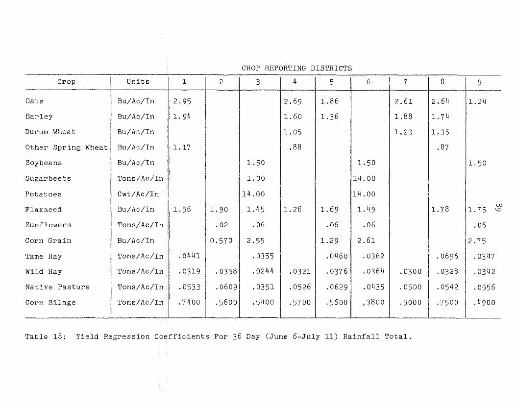
CROP REPORTING DISTRICTS

OJ

Crop Units 1 2 3 4 5 6 7 8 9

Oats Bu/Ac/In 2.95 2.69 1. 86 2.61 2.64 1. 24

Barley Bu/Ac/In 1. 94 1. 60 1.36 1.88 1. 74

Durum Wheat Bu/Ac/In 1. 05 1. 23 1. 35

Other Spring Wheat Bu/Ac/In 1.17 .88 .87

Soybeans Bu/Ac/In 1. 50 1. 50 1. 50

Sugarbeets Tons/Ac/In 1. 00 14.00

Potatoes Cwt/Ac/In 14.00 14.00

Flaxseed Bu/Ac/In 1. 56 1. 90 1.45 1.26 1. 69 1.49 1. 78 1.75

Sunflowers Tons/Ac/In .02 .06 .06 .06 .06

Corn Grain Bu/Ac/In 0.570 2.55 1. 29 2.61 2.75

Tame Hay Tons/Ac/In .0441 .0355 .0460 .0362 .0696 .0347

Wild Hay Tons/Ac/In .0319 .0358 .0244 .0321 .0376 .0364 .0300 .0328 .0342

Native Pasture Tons/Ac/In .0533 .0609 .0351 .0526 .0629 .0435 .0500 .0542 .0556

Corn Silage Tons/Ac/In .7400 .5600 .5400 .5700 .5600 ~3800 .5000 .7500 .4900

Table 18: Yield Regression Coefficients For 36 Day (June 6-July 11) Rainfall Total.

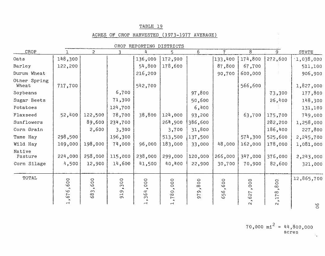
TABLE 19

ACRES OF CROP HARVESTED (1973-1977 AVERAGE)

CROP REPORTING DISTRICTSSTATE987634521CROP~~.~~ ~ ~ ~ , ~ -

Oats 148,300 136,000 172,900 133,400 1174,800 272,600 '1,038,000

Barley 122,200 54,800 178,600 87,800 67,700 511,100

Durum Wheat 216,200 90,700 600,000 906,900

Other SpringWheat 717,700 542,700 566,600 1,827,000

Soybeans 6,700 97,800 73,300 177,800

Sugar Beets 71 ,300 50,600 26,400 1118,300

Potatoes 124,700 6,400 131,100

Flaxseed 52,400 122,500 78,700 I 38,800 124,000 93,200 63,700 175,700 7 49,000

Sunflowers 89,600 234,700 264,900 386,600 282,200 1,258,000

Corn Grain 2,600 3,300 3,700 31,800 186,400 227,800

Tame Hay 298,500 196,300 513,500 137,500 574,300 525,600 2,245,700

Wild Hay 109,000 198,000 74,000 96,000 183,000 33,000 48,000 162,000 178,000 1,081,000

NativePasture 224,000 258,000 115,000 238,000 299,000 120,000 266,000 347,000 376,000 2,243,000

Corn Silage 4,500 12,900 14,600 41,500 40,400 22,900 30,700 70,900 82,600 321,000

TOTAL a a a a a a a a a 12,865,700a a a a a a a a a\D \D (Y) a a co \D a co, , , , , , , , ,\D (Y) 0'1 ~ 0. 0'1 \D t-, cor-. co r-l \D co t'-- If"\ N t'--\D \D 0'1 (Y) c-. 0'1 \D \D r-l, , , , ,r-l r-l r-l N N \D

a

70,000 mi 2 = 44,800,000acres

91

'I'ABLE 20

CROP

Oats ($/Bu)Barley ($/Bu)Durum Wheat ($/Bu)Other Spring Wheat ($/Bu)Soy Beans ($/Bu)

Sugar Beets ($/Ton)

Potatoes ($/Cwt)Flax Seed ($/Bu)Sunflowers ($/Ton)

Corn Grain ($/Bu)Tame Hay ($/Ton)

Wild Hay ($/Ton)Native Pasture ($/Ton)Corn Silage ($/Ton)

PRICE

1. 502.203.60

3.256.50

25.00

4.256.40

10.00

2.40

55.0045.0045.00

18.33

STATEDOLLAR IMPACTS*

1,202,885714,445

1,511,103

1,947,707673,026

1,965,9925,205,688

3,328,151

340,537440,128

2,357,2502,109,463

662,4921,272,899

TOTAL DIREC'I'

TOTAL (INCLUDING MULTIPLIER EFFECT)

23,731,728

71,409,872

Average annual economic impactDakota resulting from rainfall

1976-1980 for the crops shown.averages for the period.

(dollar increases) over Northenhancement during the periodPrices shown were approximate

*NOTE: The varia.tions in rainfall increase downwind fromthe target area have not been considered at this

point. When this adjustment is made, the dollarimpacts will vary accordingly.

92

each day and averaged to one value. This value for the day was

then apportioned to each CRD based on the proportion of the

CRD which was in any seeded sector. Future work will take into

account the diminishing downwind effect of the seeding and

hence reapportion the economic benefits across the state.

Using the precipitation impact and acreage information,

estimates of crop production responses were obtained. Using

these production responses and the commodity prices, estimates

of the value of the production changes were estimated. These

values are also shown in Table 20.

The information is now in hand for the input-output

analysis. The production value changes for the various crops

were aggregated into two state level categories: (1) crops

that would stimulate the crop processing sector (oats, barley,

durum wheat, other spring wheat, soybeans, sugarbeets, potatoes,

flaxseed, sunflowers, and corn grain); and (2) crops that

would stimulate the livestock sector (tame hay, wild hay,

native pasture, and corn silage). For each category, a stemming

from effect was estimated. The total direct impact would also

lead to a household consumption effect. The total direct and

indirect impact would be the sum of the total direct impacts,

and the household consumption effect. The relations among

these various effects are summarized below:

Dc = direct production value impacts forcategory (1) crops

Dl

= direct production value impacts forcategory (2) crops

SFE = 0 2285*Dc . c

93

= crop processing sectorstemming from effect

livestock sectorstemming from effect

SFEt = SFEc + SFEl = total stemming from effect

DE = Dc + Dl = total direct effect

HCE = 1.4921*DE = household consumption effect

TE = DE + SFEt + HCE = total impact.

For average condition over the whole period, these

effects are summarized in Table 21.

TABLE 21

AVERAGE STATEWIDE IMPACTS OVER 1976-1980 PERIODATTRIBUTED TO RAINFALL INCREASES FROM CLOUD SEEDING

Total Direct Impacts 23,731,728

Agricultural Processing "Stemming From" Effect....... 3,861,908

Livestock "Stemming From" Effect..................... 8,406,156

Household Consumption Effect. . . . . . . . . . . . . . . . . . . . . . . .. 35,410,096

'rOTAL EFFECT.............. 71,409,872. , ,~ ",

94

As was mentioned earlier, these figures will undergo

an adjustment when the diminishing downwind effect is in­

corporated into the economics. This will show smaller pro­

duction increases in the eastern part of the state and larger

production increases in and immediately downwind from the

seeded areas.

95

REFERENCES

Added Rainfall Effects Study Team, 1974: The Effects ofAdded Rainfall During the Growing Season in North Dakota:Final Report. North Dakota Research Report Number 52,Fargo, North Dakota, Agricultural Experiment Station,North Dakota State University.

Cooter, William S., 1980: Further Applications of Input­Output Analysis in Assessing the Effects of OperationalCloud Seeding Activities on the North Dakota Economy,AMOS EDDY, INC., Norman, Oklahoma.

Eddy, Amos, Ellen Cooter and William Cooter, 1979: AnEvaluation of Operational Cloud Seeding in North Dakota:An Exploratory Analysis. Final Contract Report toNorth Dakota Weather Modification Board, June 1979, AMOSEDDY, INC., Norman, Oklahoma.

Eddy, Amos and Ellen Cooter, 1979: The Evaluation ofOperational Cloud Seeding in North Dakota, Final Reportto North Dakota Weather Modification Board, January 1979,43 pp.

-r-r-rr-rx-r-r-r--vr-r-r-? 1978: A Drought Probability Model for theU.S.A. Northern Plains, Final Report to the Charles F.Kettering Foundation Grant No. ST 77 6.

Eddy, Amos, 1980: A Detailed Analysis of Rainfall andCloud Seeding Material for the 1977 Season Over NorthDakota, Final Report to the North Dakota Weather Modifi­cation Board by AMOS EDDY, INC.

Heffter, J. L., and A. D. Taylor, 1975: A Regional-ContinentalSc~le Transport, Diffusion, and. Deposition Model; Part 1:Trajectory Model, NOAA Tech. Memo ERL ARL-50.

Lanczos, C., 1956: Applied Analysis, Prentice Hall, 539 pp.

Palmer, W.C., 1965: Meteorological Drought, USWB, ResearchPaper No. 45, Office of Climatology, Washington, D.C.

_____--_~--, 1968: Keeping Track of Crop Moisture Conditions,Nationwide: The New Crop Moisture Index, Weatherwise.

North Dakota Crop and Livestock Reporting SerVice, 1979: NorthDakota Crop and Livestock Statistics. Agricultural StatisticsNumber 42. Fargo, North Dakota Agricultural Experiment Sta­tion, North Dakota State University.

96

Hirsch, J., 1971: Computer Modeling of Cumulus Clouds DuringProject Cloud Catcher, Institute of Atmospheric Science,South Dakota School of Mines and Technology, Report #71-7,61 pp. NTIS #PB281028/AS.

Thornthwaite, C.W., 1948: An Approach Toward a RationalClassification of Climate, Geogr. Rev., 38, pp 85-94.

United States Bureau of the Census, 1977: 1974 Census ofAgriculture: Vol. I, Part 34; North Dakota State and CountyData. Government Printing Office, Washington, D.C.