Embed Size (px)
Citation preview
arX
iv:h
ep-e
x/06
0203
5v1
20
Feb
2006
Final Report of the Muon E821 Anomalous Magnetic Moment
Measurement at BNL
G.W. Bennett2, B. Bousquet10, H.N. Brown2, G. Bunce2, R.M. Carey1, P. Cushman10,
G.T. Danby2, P.T. Debevec8, M. Deile13, H. Deng13, W. Deninger8, S.K. Dhawan13,
V.P. Druzhinin3, L. Duong10, E. Efstathiadis1, F.J.M. Farley13, G.V. Fedotovich3,
S. Giron10, F.E. Gray8, D. Grigoriev3, M. Grosse-Perdekamp13, A. Grossmann7,
M.F. Hare1, D.W. Hertzog8, X. Huang1, V.W. Hughes13†, M. Iwasaki12, K. Jungmann6,7,
D. Kawall13, M. Kawamura12, B.I. Khazin3, J. Kindem10, F. Krienen1, I. Kronkvist10,
A. Lam1, R. Larsen2, Y.Y. Lee2, I. Logashenko1,3, R. McNabb10,8, W. Meng2, J. Mi2,
J.P. Miller1, Y. Mizumachi11, W.M. Morse2, D. Nikas2, C.J.G. Onderwater8,6, Y. Orlov4,
C.S. Ozben2,8, J.M. Paley1, Q. Peng1, C.C. Polly8, J. Pretz13, R. Prigl2, G. zu Putlitz7,
T. Qian10, S.I. Redin3,13, O. Rind1, B.L. Roberts1, N. Ryskulov3, S. Sedykh8,
Y.K. Semertzidis2, P. Shagin10, Yu.M. Shatunov3, E.P. Sichtermann13, E. Solodov3,
M. Sossong8, A. Steinmetz13, L.R. Sulak1, C. Timmermans10, A. Trofimov1, D. Urner8,
P. von Walter7, D. Warburton2, D. Winn5, A. Yamamoto9 and D. Zimmerman10
(Muon (g − 2) Collaboration)
1Department of Physics, Boston University, Boston, MA 02215
2Brookhaven National Laboratory, Upton, NY 11973
3Budker Institute of Nuclear Physics, 630090 Novosibirsk, Russia
4Newman Laboratory, Cornell University, Ithaca, NY 14853
5Fairfield University, Fairfield, CT 06430
6 Kernfysisch Versneller Instituut, Rijksuniversiteit Groningen,
NL-9747 AA, Groningen, The Netherlands
7 Physikalisches Institut der Universitat Heidelberg, 69120 Heidelberg, Germany
8 Department of Physics, University of Illinois at Urbana-Champaign, Urbana, IL 61801
9 KEK, High Energy Accelerator Research Organization, Tsukuba, Ibaraki 305-0801, Japan
10Department of Physics, University of Minnesota, Minneapolis, MN 55455
11 Science University of Tokyo, Tokyo, 153-8902, Japan
† Deceased.
1
12 Tokyo Institute of Technology, 2-12-1 Ookayama, Meguro-ku, Tokyo, 152-8551, Japan
13 Department of Physics, Yale University, New Haven, CT 06520
(Dated: February 3, 2008)
Abstract
We present the final report from a series of precision measurements of the muon anomalous
magnetic moment, aµ = (g − 2)/2. The details of the experimental method, apparatus, data
taking, and analysis are summarized. Data obtained at Brookhaven National Laboratory, us-
ing nearly equal samples of positive and negative muons, were used to deduce aµ(Expt) =
11 659 208.0(5.4)(3.3) × 10−10, where the statistical and systematic uncertainties are given, re-
spectively. The combined uncertainty of 0.54 ppm represents a 14-fold improvement compared to
previous measurements at CERN. The standard model value for aµ includes contributions from
virtual QED, weak, and hadronic processes. While the QED processes account for most of the
anomaly, the largest theoretical uncertainty, ≈ 0.55 ppm, is associated with first-order hadronic
vacuum polarization. Present standard model evaluations, based on e+e− hadronic cross sections,
lie 2.2 - 2.7 standard deviations below the experimental result.
2

Contents
I. Introduction 5
II. Experimental Method 7
A. Overview 7
B. Beamline 11
C. Inflector 15
D. Muon storage ring magnet 18
E. Electric quadrupoles 19
F. Pulsed kicker magnet 24
G. Field measurement instrumentation 26
H. Detector systems, electronics and data acquisition 29
1. Electromagnetic calorimeters 29
2. Special detector systems 33
3. Waveform digitizers and special electronics 34
III. Beam Dynamics 36
A. Overview 36
B. Fast rotation 37
C. Coherent betatron oscillations 41
D. Muon losses 43
E. Electric-field and pitch correction 47
IV. Data Analysis 48
A. Determination of ωp and ωp 49
1. Absolute calibration probe 49
2. Trolley probe and plunging probe relative calibration 51
3. Measurement of azimuthal field average with trolley probes 53
4. Field tracking with the fixed probes 56
5. Average of the field over muon distribution and time 56
6. Results and systematic errors 60
B. Analysis of ωa 60
3
1. Data preparation and pulse-fitting procedure 62
2. Energy calibration and stability 66
3. Correction for multi-particle pileup 67
4. Elimination of fast rotation 70
5. Multi-parameter fitting 72
6. The ratio-fitting method 77
7. The asymmetry-weighting method 78
8. Internal and mutual consistency 78
9. Systematic errors in ωa 83
10. Consideration of a muon EDM 84
C. Final aµ result 85
V. The Standard Model Value of the Anomaly 87
VI. Discussion and Conclusions 91
VII. Acknowledgments 93
References 94
4
I. INTRODUCTION
The muon magnetic moment is related to its intrinsic spin by the gyromagnetic ratio gµ:
~µµ = gµ
( q
2m
)~S, (1)
where gµ = 2 is expected for a structureless, spin-12
particle of mass m and charge q =
±e. Radiative corrections (RC), which couple the muon spin to virtual fields, introduce an
anomalous magnetic moment defined by
aµ =1
2(gµ − 2). (2)
The leading RC is the lowest-order (LO) quantum electrodynamic process involving the
exchange of a virtual photon, the “Schwinger term,” [1] giving aµ(QED; LO) = α/2π ≈1.16× 10⁻³. The complete standard model value of aµ , currently evaluated to a precision of
approximately 0.6 ppm (parts per million), includes this first-order term along with higher-
order QED processes, electroweak loops, hadronic vacuum polarization, and other higher-
order hadronic loops. The measurement of aµ , carried out to a similar precision, is the
subject of this paper. The difference between experimental and theoretical values for aµ is a
valuable test of the completeness of the standard model. At sub-ppm precision, such a test
explores physics well above the 100 GeV scale for many standard model extensions.
The muon anomalous magnetic moment was measured in a series of three experiments
at CERN and, most recently in our E821 experiment at Brookhaven National Laboratory
(BNL). In the first CERN measurement [2] muons were injected into a 6-m long straight
magnet where they followed a drifting spiral path, slowly traversing the magnet because
of a small gradient introduced in the field. The muons were stopped in a polarimeter
outside the magnet and a measurement of their net spin precession determined aµ with an
uncertainty of 4300 ppm. The result agreed with the prediction of QED for a structureless
particle. The second CERN experiment [3] used a magnetic ring to extend the muon storage
time. A primary proton beam was injected directly onto a target inside the storage ring
where produced pions decayed to muons, a small fraction of which fell onto stable orbits.
The muon precession frequency was determined by a sinusoidal modulation in the time
distribution of decay positrons, measured by detectors on the opposite side of the ring
from the injection point. The result to 270 ppm agreed with QED only after the theory
5
had been recalculated [4]. The CERN-III experiment [5] used a uniform-field storage ring
and electric quadrupoles to provide vertical containment for the muons having the “magic”
momentum of 3.1 GeV/c. At this momentum, the muon spin precession is not affected by
the electric field from the focusing quadrupoles. Additionally, pions were injected directly
into the ring, which resulted in a higher stored muon fraction and less background than
proton injection. The CERN-III experiment achieved a precision of 10 ppm for each muon
polarity. CPT symmetry was assumed, and the results were combined to give a 7.3 ppm
measurement, which agreed with theory. The result served as the first confirmation of the
predicted 60 ppm contribution to aµ from hadronic vacuum polarization.
The present BNL experiment follows the general technique pioneered by CERN-III, but
features many innovative improvements. A continuous superconducting magnet, having high
field uniformity, is used instead of a lattice of discrete resistive magnets. A direct current,
rather than pulsed, inflector magnet permits the ring to be filled at 33 ms intervals, the
bunch extraction interval from the AGS. Muons are injected directly into the storage ring,
which increases the storage efficiency and reduces the intense hadron-induced background
“flash.” A pulsed kicker places the muons onto stable orbits and centers them in the storage
region. The electrostatic quadrupoles permit operation at about twice the field gradient
of the CERN experiment. The transverse aperture of the storage region is circular rather
than rectangular, in order to reduce the dependence of the average field seen by a muon
on its trajectory. The magnetic field is mapped using an array of NMR probes, mounted
on a trolley that can be pulled through the vacuum chamber. Waveform digitizers provide
a time record of energy deposition in calorimeters. The records are used to determine
electron energies and times and to correct for multi-particle overlap–“pileup.” (Note: In
this manuscript, we use electron to represent either the positron or electron in the generic
µ→ eνν decay chain.)
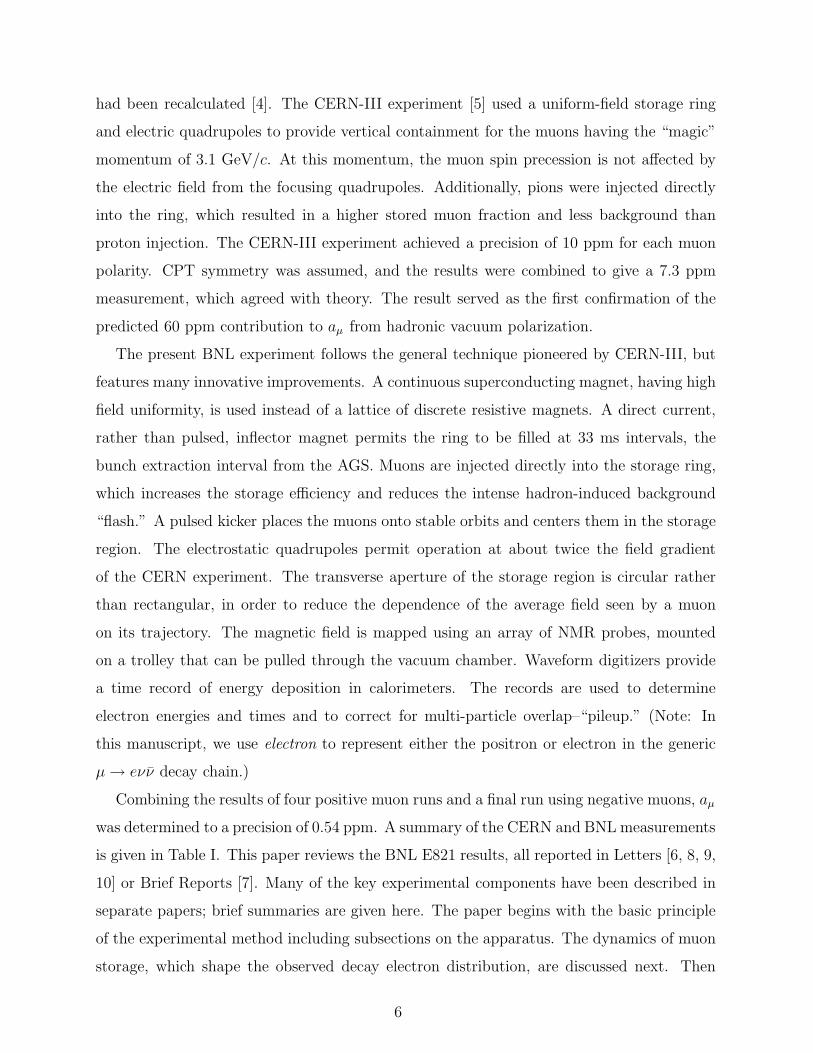
Combining the results of four positive muon runs and a final run using negative muons, aµ
was determined to a precision of 0.54 ppm. A summary of the CERN and BNL measurements
is given in Table I. This paper reviews the BNL E821 results, all reported in Letters [6, 8, 9,
10] or Brief Reports [7]. Many of the key experimental components have been described in
separate papers; brief summaries are given here. The paper begins with the basic principle
of the experimental method including subsections on the apparatus. The dynamics of muon
storage, which shape the observed decay electron distribution, are discussed next. Then
6
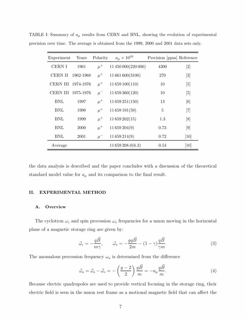
TABLE I: Summary of aµ results from CERN and BNL, showing the evolution of experimental
precision over time. The average is obtained from the 1999, 2000 and 2001 data sets only.
Experiment Years Polarity aµ × 1010 Precision [ppm] Reference
CERN I 1961 µ+ 11 450 000(220 000) 4300 [2]
CERN II 1962-1968 µ+ 11 661 600(3100) 270 [3]
CERN III 1974-1976 µ+ 11 659 100(110) 10 [5]
CERN III 1975-1976 µ− 11 659 360(120) 10 [5]
BNL 1997 µ+ 11 659 251(150) 13 [6]
BNL 1998 µ+ 11 659 191(59) 5 [7]
BNL 1999 µ+ 11 659 202(15) 1.3 [8]
BNL 2000 µ+ 11 659 204(9) 0.73 [9]
BNL 2001 µ− 11 659 214(9) 0.72 [10]
Average 11 659 208.0(6.3) 0.54 [10]
the data analysis is described and the paper concludes with a discussion of the theoretical
standard model value for aµ and its comparison to the final result.
II. EXPERIMENTAL METHOD
A. Overview
The cyclotron ωc and spin precession ωs frequencies for a muon moving in the horizontal
plane of a magnetic storage ring are given by:
~ωc = − q ~B
mγ, ~ωs = −gq
~B
2m− (1 − γ)
q ~B
γm. (3)
The anomalous precession frequency ωa is determined from the difference
~ωa = ~ωs − ~ωc = −(g − 2
2
)q ~B
m= −aµ
q ~B
m. (4)
Because electric quadrupoles are used to provide vertical focusing in the storage ring, their
electric field is seen in the muon rest frame as a motional magnetic field that can affect the
7
spin precession frequency. In the presence of both ~E and ~B fields, and in the case that ~β
is perpendicular to both ~E and ~B, the expression for the anomalous precession frequency
becomes
~ωa = − q
m
[aµ~B −
(aµ − 1
γ2 − 1
) ~β × ~E
c
]. (5)
The coefficient of the ~β× ~E term vanishes at the “magic” momentum of 3.094 GeV/c, where
γ = 29.3. Thus aµ can be determined by a precision measurement of ωa and B. At this
magic momentum, the electric field is used only for muon storage and the magnetic field
alone determines the precession frequency. The finite spread in beam momentum and vertical
betatron oscillations introduce small (sub ppm) corrections to the precession frequency.
The longitudinally polarized muons, which are injected into the storage ring at the magic
momentum, have a time-dilated muon lifetime of 64.4 µs. A measurement period of typically
700 µs follows each injection or “fill.” The net spin precession depends on the integrated
field seen by a muon along its trajectory. The magnetic field used in Eq. 5 refers to an
average over muon trajectories during the course of the experiment. The trajectories of the
muons must be weighted with the magnetic field distribution. To minimize the precision
with which the average particle trajectories must be known, the field should be made as
uniform as possible.
Because of parity violation in the weak decay of the muon, a correlation existsbetween
the muon spin and decay electron direction. This correlation allows the spin direction to
be measured as a function of time. In the rest frame of the muon—indicated by starred
quantities—the differential probability for the electron to emerge with a normalized energy
y = E∗/Emax (Emax = 52.8 MeV) at an angle θ∗ with respect to the muon spin is [11]
dP (y, θ∗)
dy dΩ= (1/2π)n∗(y)[1 − α∗(y) cos θ∗] with (6)
n∗(y) = y2(3 − 2y) and (7)
α∗(y) =q
e
2y − 1
3 − 2y. (8)
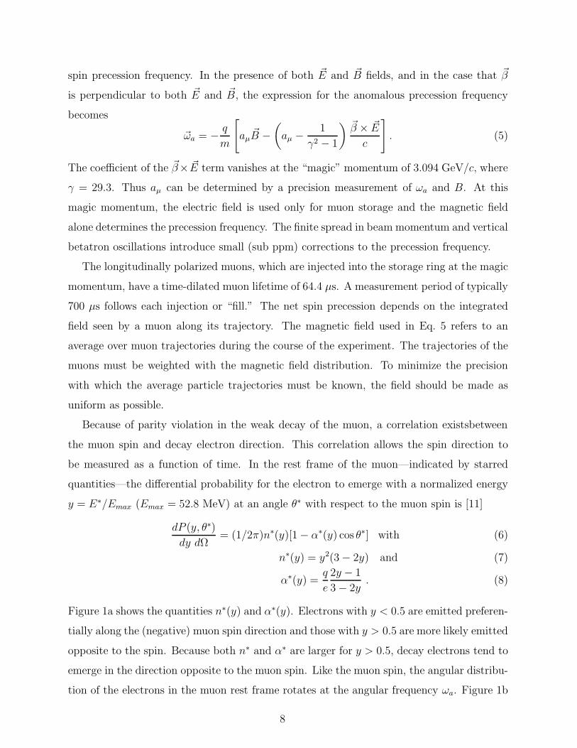
Figure 1a shows the quantities n∗(y) and α∗(y). Electrons with y < 0.5 are emitted preferen-
tially along the (negative) muon spin direction and those with y > 0.5 are more likely emitted
opposite to the spin. Because both n∗ and α∗ are larger for y > 0.5, decay electrons tend to
emerge in the direction opposite to the muon spin. Like the muon spin, the angular distribu-
tion of the electrons in the muon rest frame rotates at the angular frequency ωa. Figure 1b
8
y0 0.1 0.2 0.3 0.4 0.5 0.6 0.7 0.8 0.9 1
Rel
ativ
e N
um
ber
(n
) o
r A
sym
met
ry (
A)
-0.2
0
0.2
0.4
0.6
0.8
1
n(y)
A(y)(y)α*
n (y)*
(a) Center-of-mass frame
y0 0.1 0.2 0.3 0.4 0.5 0.6 0.7 0.8 0.9 1
No
rmal
ized
nu
mb
er (
N)
or
Asy
mm
etry
(A
)
-0.2
0
0.2
0.4
0.6
0.8
1N
A
NA2
(b) Lab frame
FIG. 1: Relative number and asymmetry distributions versus electron fractional energy y in the
muon rest frame (left panel) and in the laboratory frame (right panel). The differential figure-of-
merit product NA2 in the laboratory frame illustrates the importance of the higher-energy electrons
in reducing the measurement statistical uncertainty.
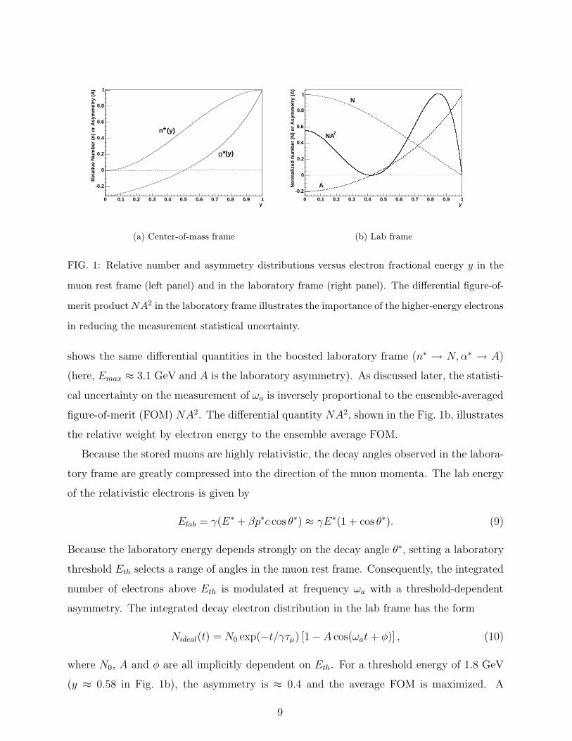
shows the same differential quantities in the boosted laboratory frame (n∗ → N,α∗ → A)
(here, Emax ≈ 3.1 GeV and A is the laboratory asymmetry). As discussed later, the statisti-
cal uncertainty on the measurement of ωa is inversely proportional to the ensemble-averaged
figure-of-merit (FOM) NA2. The differential quantity NA2, shown in the Fig. 1b, illustrates
the relative weight by electron energy to the ensemble average FOM.
Because the stored muons are highly relativistic, the decay angles observed in the labora-
tory frame are greatly compressed into the direction of the muon momenta. The lab energy
of the relativistic electrons is given by
Elab = γ(E∗ + βp∗c cos θ∗) ≈ γE∗(1 + cos θ∗). (9)
Because the laboratory energy depends strongly on the decay angle θ∗, setting a laboratory
threshold Eth selects a range of angles in the muon rest frame. Consequently, the integrated
number of electrons above Eth is modulated at frequency ωa with a threshold-dependent
asymmetry. The integrated decay electron distribution in the lab frame has the form
Nideal(t) = N0 exp(−t/γτµ) [1 − A cos(ωat+ φ)] , (10)
where N0, A and φ are all implicitly dependent on Eth. For a threshold energy of 1.8 GeV
(y ≈ 0.58 in Fig. 1b), the asymmetry is ≈ 0.4 and the average FOM is maximized. A
9
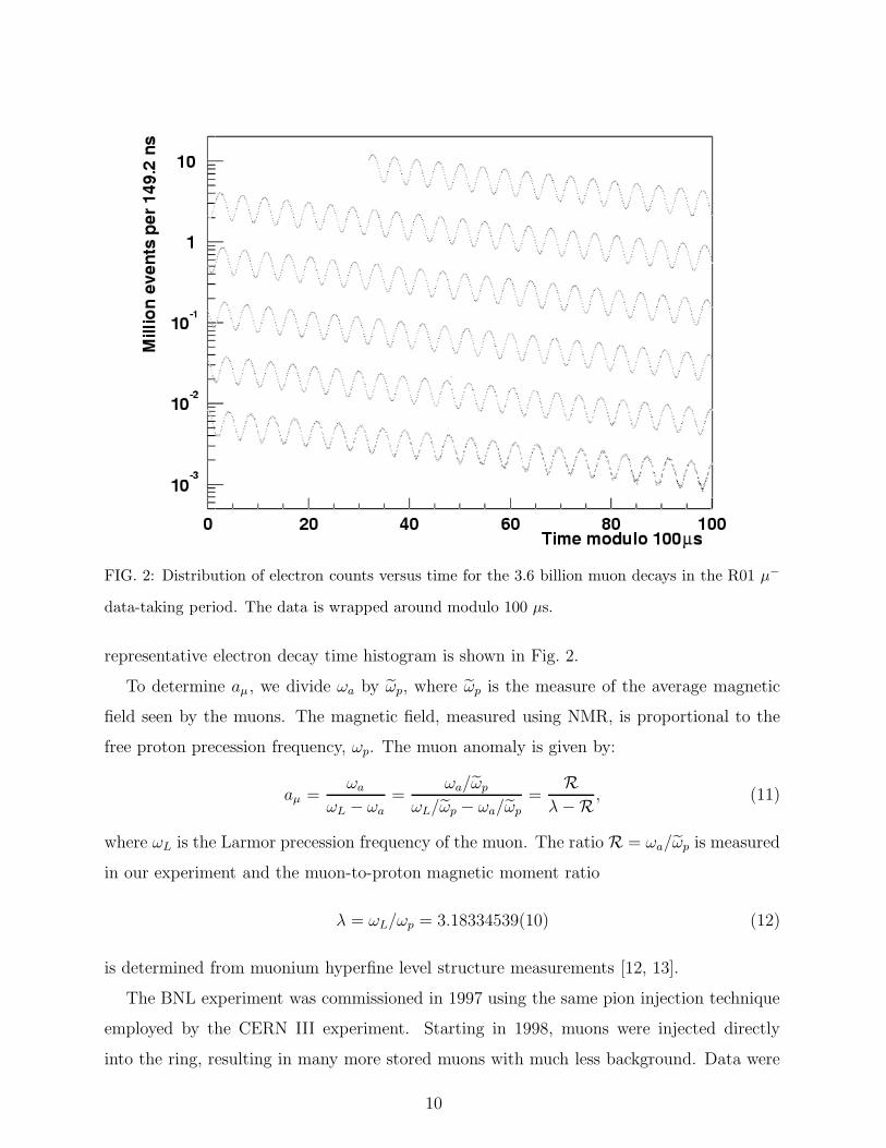
FIG. 2: Distribution of electron counts versus time for the 3.6 billion muon decays in the R01 µ−
data-taking period. The data is wrapped around modulo 100 µs.
representative electron decay time histogram is shown in Fig. 2.
To determine aµ , we divide ωa by ωp, where ωp is the measure of the average magnetic
field seen by the muons. The magnetic field, measured using NMR, is proportional to the
free proton precession frequency, ωp. The muon anomaly is given by:
aµ =ωa
ωL − ωa
=ωa/ωp
ωL/ωp − ωa/ωp
=R
λ−R , (11)
where ωL is the Larmor precession frequency of the muon. The ratio R = ωa/ωp is measured
in our experiment and the muon-to-proton magnetic moment ratio
λ = ωL/ωp = 3.18334539(10) (12)
is determined from muonium hyperfine level structure measurements [12, 13].
The BNL experiment was commissioned in 1997 using the same pion injection technique
employed by the CERN III experiment. Starting in 1998, muons were injected directly
into the ring, resulting in many more stored muons with much less background. Data were
10
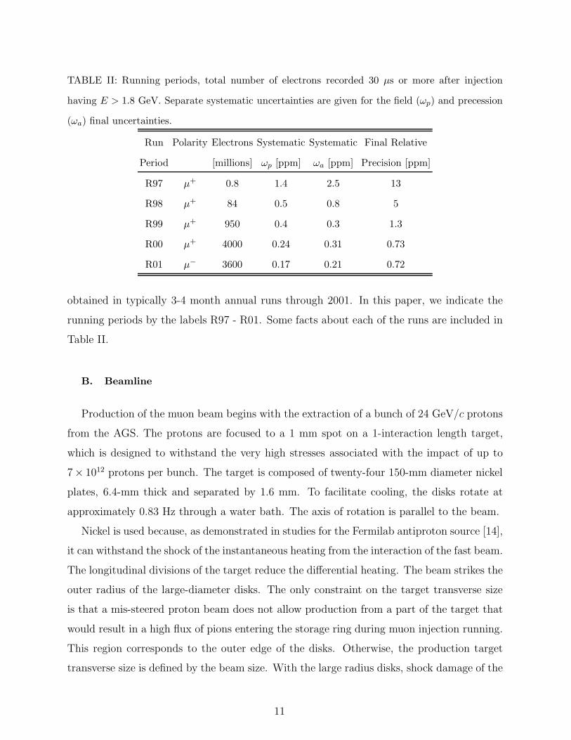
TABLE II: Running periods, total number of electrons recorded 30 µs or more after injection
having E > 1.8 GeV. Separate systematic uncertainties are given for the field (ωp) and precession
(ωa) final uncertainties.
Run Polarity Electrons Systematic Systematic Final Relative
Period [millions] ωp [ppm] ωa [ppm] Precision [ppm]
R97 µ+ 0.8 1.4 2.5 13
R98 µ+ 84 0.5 0.8 5
R99 µ+ 950 0.4 0.3 1.3
R00 µ+ 4000 0.24 0.31 0.73
R01 µ− 3600 0.17 0.21 0.72
obtained in typically 3-4 month annual runs through 2001. In this paper, we indicate the
running periods by the labels R97 - R01. Some facts about each of the runs are included in
Table II.
B. Beamline
Production of the muon beam begins with the extraction of a bunch of 24 GeV/c protons
from the AGS. The protons are focused to a 1 mm spot on a 1-interaction length target,
which is designed to withstand the very high stresses associated with the impact of up to
7× 10¹² protons per bunch. The target is composed of twenty-four 150-mm diameter nickel
plates, 6.4-mm thick and separated by 1.6 mm. To facilitate cooling, the disks rotate at
approximately 0.83 Hz through a water bath. The axis of rotation is parallel to the beam.
Nickel is used because, as demonstrated in studies for the Fermilab antiproton source [14],
it can withstand the shock of the instantaneous heating from the interaction of the fast beam.
The longitudinal divisions of the target reduce the differential heating. The beam strikes the
outer radius of the large-diameter disks. The only constraint on the target transverse size
is that a mis-steered proton beam does not allow production from a part of the target that
would result in a high flux of pions entering the storage ring during muon injection running.
This region corresponds to the outer edge of the disks. Otherwise, the production target
transverse size is defined by the beam size. With the large radius disks, shock damage of the
11
target is distributed over the disk circumference as the disks rotate. Still, it was necessary
to replace the target after each running period, typically following an exposure of 5 × 10¹⁹
protons, or when nickel dust was observed in the target water cooling basin.
Pions are collected from the primary target at zero angle and transferred into a secondary
pion-muon decay channel, designed to maximize the flux of polarized muons while minimiz-
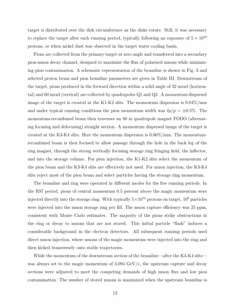
ing pion contamination. A schematic representation of the beamline is shown in Fig. 3 and
selected proton beam and pion beamline parameters are given in Table III. Downstream of
the target, pions produced in the forward direction within a solid angle of 32 mrad (horizon-
tal) and 60 mrad (vertical) are collected by quadrupoles Q1 and Q2. A momentum-dispersed
image of the target is created at the K1-K2 slits. The momentum dispersion is 0.04%/mm
and under typical running conditions the pion momentum width was δp/p ∼ ±0.5%. The
momentum-recombined beam then traverses an 80 m quadrupole magnet FODO (alternat-
ing focusing and defocusing) straight section. A momentum dispersed image of the target is
created at the K3-K4 slits. Here the momentum dispersion is 0.06%/mm. The momentum-
recombined beam is then focused to allow passage through the hole in the back leg of the
ring magnet, through the strong vertically focusing storage ring fringing field, the inflector,
and into the storage volume. For pion injection, the K1-K2 slits select the momentum of
the pion beam and the K3-K4 slits are effectively not used. For muon injection, the K3-K4
slits reject most of the pion beam and select particles having the storage ring momentum.
The beamline and ring were operated in different modes for the five running periods. In
the R97 period, pions of central momentum 0.5 percent above the magic momentum were
injected directly into the storage ring. With typically 5×10¹² protons on target, 108 particles
were injected into the muon storage ring per fill. The muon capture efficiency was 25 ppm,
consistent with Monte Carlo estimates. The majority of the pions strike obstructions in
the ring or decay to muons that are not stored. This initial particle “flash” induces a
considerable background in the electron detectors. All subsequent running periods used
direct muon injection, where muons of the magic momentum were injected into the ring and
then kicked transversely onto stable trajectories.
While the momentum of the downstream section of the beamline—after the K3-K4 slits—
was always set to the magic momentum of 3.094 GeV/c, the upstream capture and decay
sections were adjusted to meet the competing demands of high muon flux and low pion
contamination. The number of stored muons is maximized when the upstream beamline is
12
D5U line
D3,
D4
Q2
Q1
D6
D1,D2
V line
AGS
VD3
VD4
Beam Stop
Inflector
Pion Decay Channel
Pion Production Target
K1−K2
K3−
K4
2 Ringg −
U V line−
FIG. 3: Plan view of the pion/muon beamline. The pion decay channel is 80 m and the ring
diameter is 14.1 m.
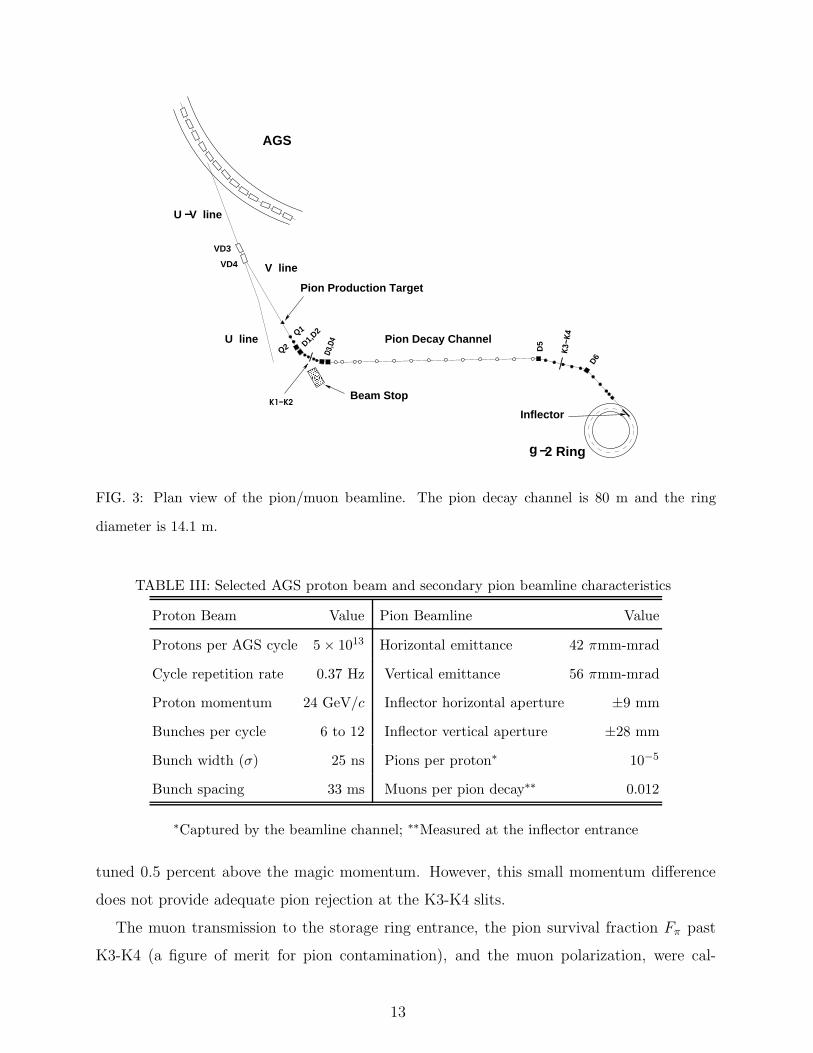
TABLE III: Selected AGS proton beam and secondary pion beamline characteristics
Proton Beam Value Pion Beamline Value
Protons per AGS cycle 5 × 10¹³ Horizontal emittance 42 πmm-mrad
Cycle repetition rate 0.37 Hz Vertical emittance 56 πmm-mrad
Proton momentum 24 GeV/c Inflector horizontal aperture ±9 mm
Bunches per cycle 6 to 12 Inflector vertical aperture ±28 mm
Bunch width (σ) 25 ns Pions per proton∗ 10−5
Bunch spacing 33 ms Muons per pion decay∗∗ 0.012
∗Captured by the beamline channel; ∗∗Measured at the inflector entrance
tuned 0.5 percent above the magic momentum. However, this small momentum difference
does not provide adequate pion rejection at the K3-K4 slits.
The muon transmission to the storage ring entrance, the pion survival fraction Fπ past
K3-K4 (a figure of merit for pion contamination), and the muon polarization, were cal-
13
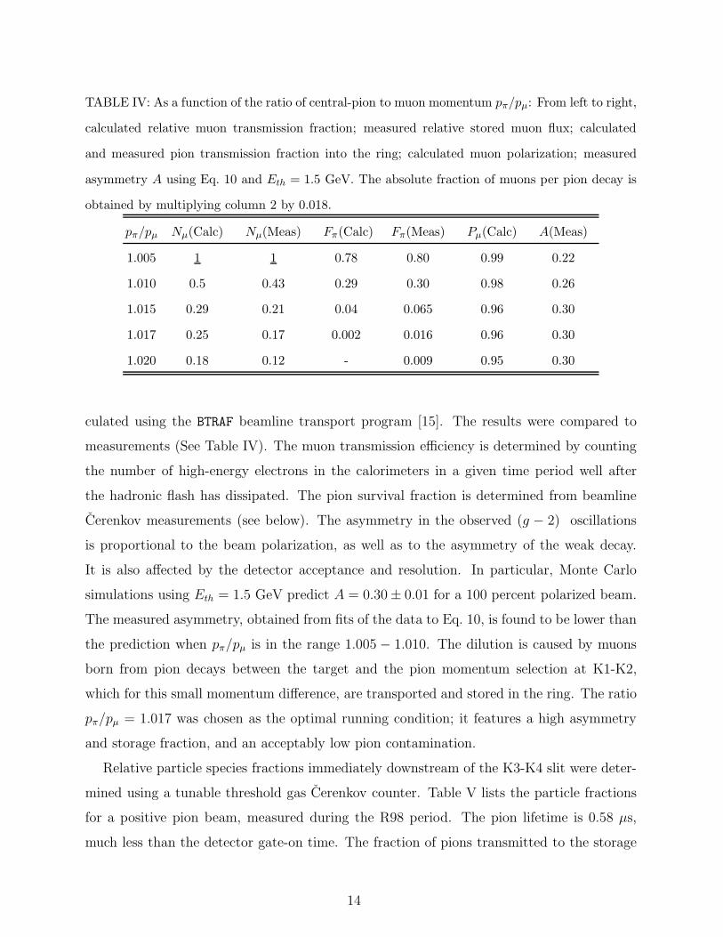
TABLE IV: As a function of the ratio of central-pion to muon momentum pπ/pµ: From left to right,
calculated relative muon transmission fraction; measured relative stored muon flux; calculated
and measured pion transmission fraction into the ring; calculated muon polarization; measured
asymmetry A using Eq. 10 and Eth = 1.5 GeV. The absolute fraction of muons per pion decay is
obtained by multiplying column 2 by 0.018.
pπ/pµ Nµ(Calc) Nµ(Meas) Fπ(Calc) Fπ(Meas) Pµ(Calc) A(Meas)
1.005 1 1 0.78 0.80 0.99 0.22
1.010 0.5 0.43 0.29 0.30 0.98 0.26
1.015 0.29 0.21 0.04 0.065 0.96 0.30
1.017 0.25 0.17 0.002 0.016 0.96 0.30
1.020 0.18 0.12 - 0.009 0.95 0.30
culated using the BTRAF beamline transport program [15]. The results were compared to
measurements (See Table IV). The muon transmission efficiency is determined by counting
the number of high-energy electrons in the calorimeters in a given time period well after
the hadronic flash has dissipated. The pion survival fraction is determined from beamline
Cerenkov measurements (see below). The asymmetry in the observed (g − 2) oscillations
is proportional to the beam polarization, as well as to the asymmetry of the weak decay.
It is also affected by the detector acceptance and resolution. In particular, Monte Carlo
simulations using Eth = 1.5 GeV predict A = 0.30± 0.01 for a 100 percent polarized beam.
The measured asymmetry, obtained from fits of the data to Eq. 10, is found to be lower than
the prediction when pπ/pµ is in the range 1.005 − 1.010. The dilution is caused by muons
born from pion decays between the target and the pion momentum selection at K1-K2,
which for this small momentum difference, are transported and stored in the ring. The ratio
pπ/pµ = 1.017 was chosen as the optimal running condition; it features a high asymmetry
and storage fraction, and an acceptably low pion contamination.
Relative particle species fractions immediately downstream of the K3-K4 slit were deter-
mined using a tunable threshold gas Cerenkov counter. Table V lists the particle fractions
for a positive pion beam, measured during the R98 period. The pion lifetime is 0.58 µs,
much less than the detector gate-on time. The fraction of pions transmitted to the storage
14
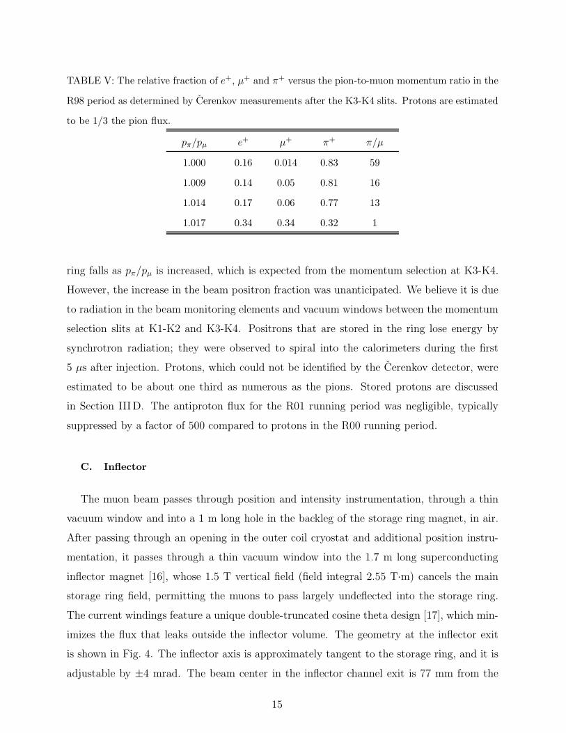
TABLE V: The relative fraction of e+, µ+ and π+ versus the pion-to-muon momentum ratio in the
R98 period as determined by Cerenkov measurements after the K3-K4 slits. Protons are estimated
to be 1/3 the pion flux.
pπ/pµ e+ µ+ π+ π/µ
1.000 0.16 0.014 0.83 59
1.009 0.14 0.05 0.81 16
1.014 0.17 0.06 0.77 13
1.017 0.34 0.34 0.32 1
ring falls as pπ/pµ is increased, which is expected from the momentum selection at K3-K4.
However, the increase in the beam positron fraction was unanticipated. We believe it is due
to radiation in the beam monitoring elements and vacuum windows between the momentum
selection slits at K1-K2 and K3-K4. Positrons that are stored in the ring lose energy by
synchrotron radiation; they were observed to spiral into the calorimeters during the first
5 µs after injection. Protons, which could not be identified by the Cerenkov detector, were
estimated to be about one third as numerous as the pions. Stored protons are discussed
in Section IIID. The antiproton flux for the R01 running period was negligible, typically
suppressed by a factor of 500 compared to protons in the R00 running period.
C. Inflector
The muon beam passes through position and intensity instrumentation, through a thin
vacuum window and into a 1 m long hole in the backleg of the storage ring magnet, in air.
After passing through an opening in the outer coil cryostat and additional position instru-
mentation, it passes through a thin vacuum window into the 1.7 m long superconducting
inflector magnet [16], whose 1.5 T vertical field (field integral 2.55 T·m) cancels the main
storage ring field, permitting the muons to pass largely undeflected into the storage ring.
The current windings feature a unique double-truncated cosine theta design [17], which min-
imizes the flux that leaks outside the inflector volume. The geometry at the inflector exit
is shown in Fig. 4. The inflector axis is approximately tangent to the storage ring, and it is
adjustable by ±4 mrad. The beam center in the inflector channel exit is 77 mm from the
15
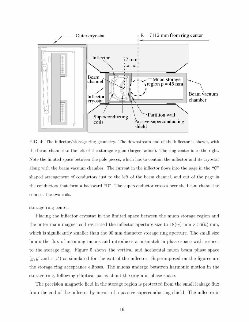
FIG. 4: The inflector/storage ring geometry. The downstream end of the inflector is shown, with
the beam channel to the left of the storage region (larger radius). The ring center is to the right.
Note the limited space between the pole pieces, which has to contain the inflector and its cryostat
along with the beam vacuum chamber. The current in the inflector flows into the page in the “C”
shaped arrangement of conductors just to the left of the beam channel, and out of the page in
the conductors that form a backward “D”. The superconductor crosses over the beam channel to
connect the two coils.
storage-ring center.
Placing the inflector cryostat in the limited space between the muon storage region and
the outer main magnet coil restricted the inflector aperture size to 18(w) mm × 56(h) mm,
which is significantly smaller than the 90 mm diameter storage ring aperture. The small size
limits the flux of incoming muons and introduces a mismatch in phase space with respect
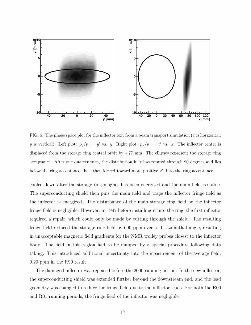
to the storage ring. Figure 5 shows the vertical and horizontal muon beam phase space
(y, y′ and x, x′) as simulated for the exit of the inflector. Superimposed on the figures are
the storage ring acceptance ellipses. The muons undergo betatron harmonic motion in the
storage ring, following elliptical paths about the origin in phase space.
The precision magnetic field in the storage region is protected from the small leakage flux
from the end of the inflector by means of a passive superconducting shield. The inflector is
16
y [mm]-40 -20 0 20 40
y’ [
mra
d]
-10
-5
0
5
10
x [mm]-40 -20 0 20 40 60 80 100 120
x’ [
mra
d]
-10
-5
0
5
10
FIG. 5: The phase space plot for the inflector exit from a beam transport simulation (x is horizontal;
y is vertical). Left plot: py/pz = y′ vs. y. Right plot: px/pz = x′ vs. x. The inflector center is
displaced from the storage ring central orbit by +77 mm. The ellipses represent the storage ring
acceptance. After one quarter turn, the distribution in x has rotated through 90 degrees and lies
below the ring acceptance. It is then kicked toward more positive x′, into the ring acceptance.
cooled down after the storage ring magnet has been energized and the main field is stable.
The superconducting shield then pins the main field and traps the inflector fringe field as
the inflector is energized. The disturbance of the main storage ring field by the inflector
fringe field is negligible. However, in 1997 before installing it into the ring, the first inflector
required a repair, which could only be made by cutting through the shield. The resulting
fringe field reduced the storage ring field by 600 ppm over a 1 azimuthal angle, resulting
in unacceptable magnetic field gradients for the NMR trolley probes closest to the inflector
body. The field in this region had to be mapped by a special procedure following data
taking. This introduced additional uncertainty into the measurement of the average field,
0.20 ppm in the R99 result.
The damaged inflector was replaced before the 2000 running period. In the new inflector,
the superconducting shield was extended further beyond the downstream end, and the lead
geometry was changed to reduce the fringe field due to the inflector leads. For both the R00
and R01 running periods, the fringe field of the inflector was negligible.
17
D. Muon storage ring magnet
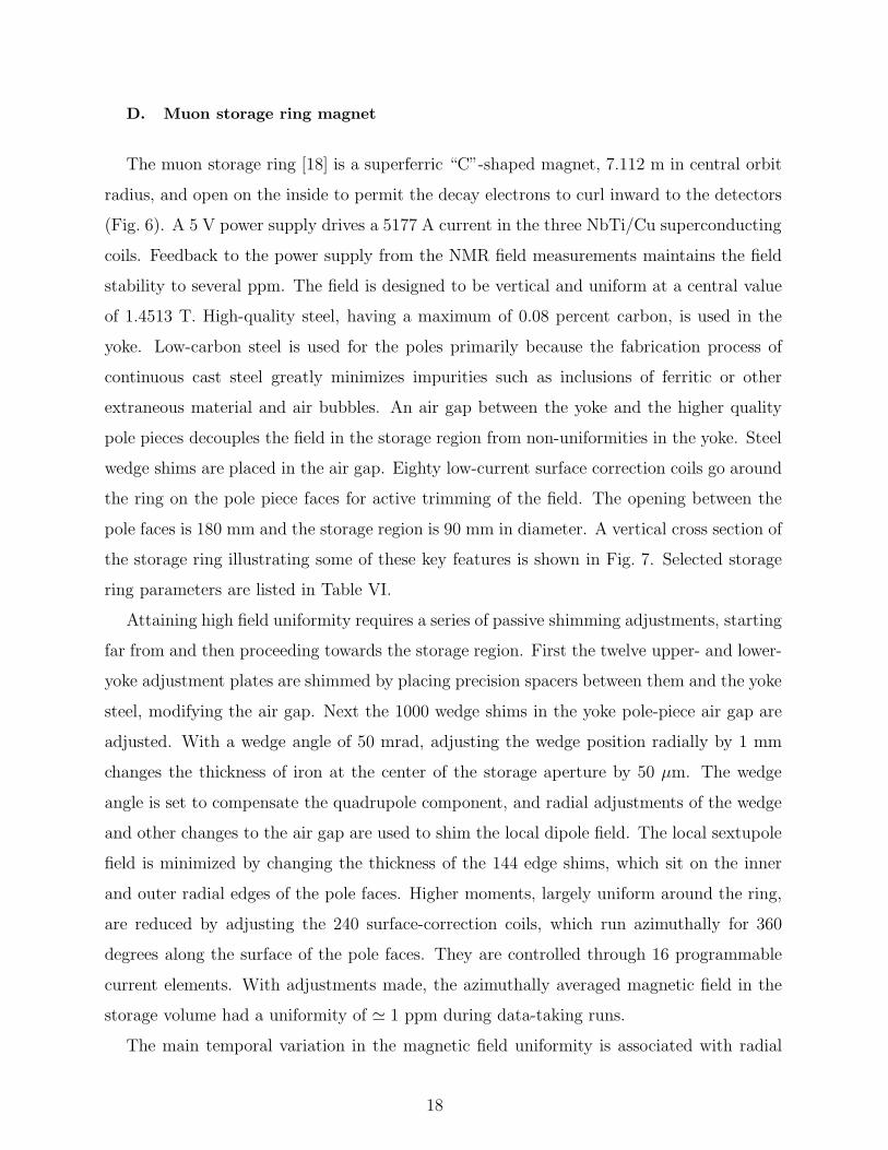
The muon storage ring [18] is a superferric “C”-shaped magnet, 7.112 m in central orbit
radius, and open on the inside to permit the decay electrons to curl inward to the detectors
(Fig. 6). A 5 V power supply drives a 5177 A current in the three NbTi/Cu superconducting
coils. Feedback to the power supply from the NMR field measurements maintains the field
stability to several ppm. The field is designed to be vertical and uniform at a central value
of 1.4513 T. High-quality steel, having a maximum of 0.08 percent carbon, is used in the
yoke. Low-carbon steel is used for the poles primarily because the fabrication process of
continuous cast steel greatly minimizes impurities such as inclusions of ferritic or other
extraneous material and air bubbles. An air gap between the yoke and the higher quality
pole pieces decouples the field in the storage region from non-uniformities in the yoke. Steel
wedge shims are placed in the air gap. Eighty low-current surface correction coils go around
the ring on the pole piece faces for active trimming of the field. The opening between the
pole faces is 180 mm and the storage region is 90 mm in diameter. A vertical cross section of
the storage ring illustrating some of these key features is shown in Fig. 7. Selected storage
ring parameters are listed in Table VI.
Attaining high field uniformity requires a series of passive shimming adjustments, starting
far from and then proceeding towards the storage region. First the twelve upper- and lower-
yoke adjustment plates are shimmed by placing precision spacers between them and the yoke
steel, modifying the air gap. Next the 1000 wedge shims in the yoke pole-piece air gap are
adjusted. With a wedge angle of 50 mrad, adjusting the wedge position radially by 1 mm
changes the thickness of iron at the center of the storage aperture by 50 µm. The wedge
angle is set to compensate the quadrupole component, and radial adjustments of the wedge
and other changes to the air gap are used to shim the local dipole field. The local sextupole
field is minimized by changing the thickness of the 144 edge shims, which sit on the inner
and outer radial edges of the pole faces. Higher moments, largely uniform around the ring,
are reduced by adjusting the 240 surface-correction coils, which run azimuthally for 360
degrees along the surface of the pole faces. They are controlled through 16 programmable
current elements. With adjustments made, the azimuthally averaged magnetic field in the
storage volume had a uniformity of ≃ 1 ppm during data-taking runs.
The main temporal variation in the magnetic field uniformity is associated with radial
18
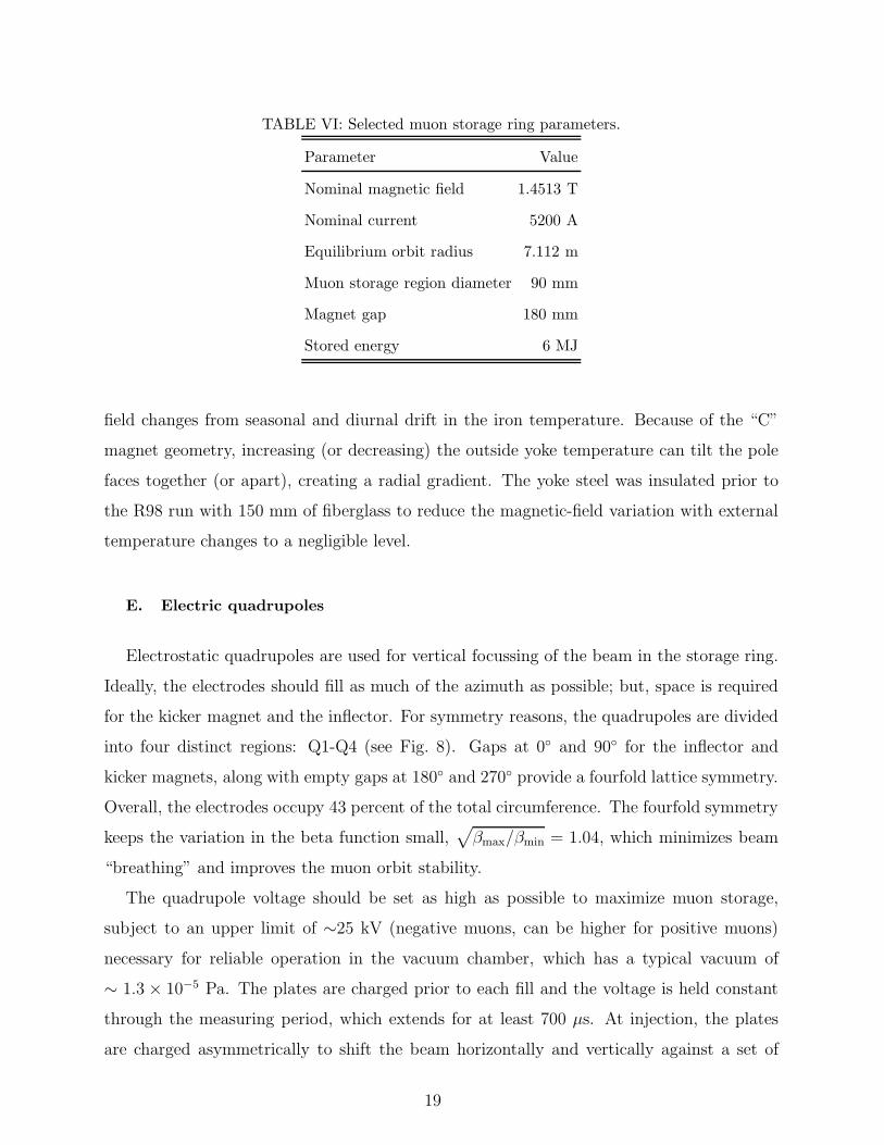
TABLE VI: Selected muon storage ring parameters.
Parameter Value
Nominal magnetic field 1.4513 T
Nominal current 5200 A
Equilibrium orbit radius 7.112 m
Muon storage region diameter 90 mm
Magnet gap 180 mm
Stored energy 6 MJ
field changes from seasonal and diurnal drift in the iron temperature. Because of the “C”
magnet geometry, increasing (or decreasing) the outside yoke temperature can tilt the pole
faces together (or apart), creating a radial gradient. The yoke steel was insulated prior to
the R98 run with 150 mm of fiberglass to reduce the magnetic-field variation with external
temperature changes to a negligible level.
E. Electric quadrupoles
Electrostatic quadrupoles are used for vertical focussing of the beam in the storage ring.
Ideally, the electrodes should fill as much of the azimuth as possible; but, space is required
for the kicker magnet and the inflector. For symmetry reasons, the quadrupoles are divided
into four distinct regions: Q1-Q4 (see Fig. 8). Gaps at 0 and 90 for the inflector and
kicker magnets, along with empty gaps at 180 and 270 provide a fourfold lattice symmetry.
Overall, the electrodes occupy 43 percent of the total circumference. The fourfold symmetry
keeps the variation in the beta function small,√βmax/βmin = 1.04, which minimizes beam
“breathing” and improves the muon orbit stability.
The quadrupole voltage should be set as high as possible to maximize muon storage,
subject to an upper limit of ∼25 kV (negative muons, can be higher for positive muons)
necessary for reliable operation in the vacuum chamber, which has a typical vacuum of
∼ 1.3 × 10⁻⁵ Pa. The plates are charged prior to each fill and the voltage is held constant
through the measuring period, which extends for at least 700 µs. At injection, the plates
are charged asymmetrically to shift the beam horizontally and vertically against a set of
19
FIG. 6: A 3D engineering rendition of the E821 muon storage ring. Muons enter the back of
the storage ring through a field-free channel at approximately 10 o’clock in the figure. The three
kicker modulators at approximately 2 o’clock provide the short current pulse, which gives the
muon bunch a transverse 10 mrad kick. The regularly spaced boxes on rails represent the electron
detector systems.
centered circular collimators—the scraping procedure. Approximately 5 − 15 µs later, the
plate voltages are symmetrized to enable long-term muon storage. The operating voltages,
field indices (which are proportional to the quadrupole gradient), the initial asymmetric
scraping time, and the total pulse length are given in Table VII.
A schematic representation of a cross section of the electrostatic quadrupole electrodes [19]
is shown in Fig. 9. The four trolley rails are at ground potential. Flat, rather than hyperbolic,
electrodes are used because they are easier to fabricate. With flat electrodes, electric-field
multipoles 8, 12, 16, · · · in addition to the quadrupole are allowed by the four-fold symmetry
(see Fig. 9). Of these, the 12- and 20-pole components are the largest. The ratio of the
width (47 mm) of the electrode to the distance between opposite plates (100 mm) is set
to minimize the 12-pole component. Beam dynamics simulations indicated that even the
20
Shim plateThrough bolt
Iron yoke
slotOuter coil
Spacer Plates
1570 mm
544 mm
Inner upper coil
Poles
Inner lower coil
To ring center
Muon beam
Upper push−rod
1394 mm
360 mm
FIG. 7: Cross sectional view of the “C” magnet.
largest of the resulting multipoles, a 2 percent 20-pole component (at the circular edge of
the storage region), would not cause problems with muon losses or beam instabilities at the
chosen values of the field indices. The scalloped vacuum chamber introduces small 6- and
10-pole multipoles into the field shape.
The quadrupoles are charged for ≤ 1.4 ms of data taking during each fill of the ring.
Cycling the quadrupoles prevents the excessive buildup of electrons around the electrodes,
electrons which are produced by field emission and gas ionization and subsequently trapped
in the electric and magnetic fields near the quadrupoles. Trapping was particularly severe
during the R01 running period when negative muons were injected into the ring. The con-
tinuous motion of the electrons—cyclotron motion in the dipole magnetic field, magnetron
motion along ~E × ~B, and axial oscillations along the vertical axis—ionizes the residual gas
and eventually produces a spark, which discharges the plates.
Slight modifications of the magnetron motion were used to quench the electron trapping.
In the original design, electrons undergoing magnetron motion were trapped in horizontal
21
12
3
4
5
6
7
8
9
10
11
121314
15
16
17
18
19
20
21
22
23
24
212
1
21
21
21180 Fiber
monitor
garageTrolley
chambersTraceback
270 Fibermonitor
K1
K2
K3
Q1
C
C
InflectorC
CalibrationNMR probe
C
CC
C
Q4
CQ2
Q3
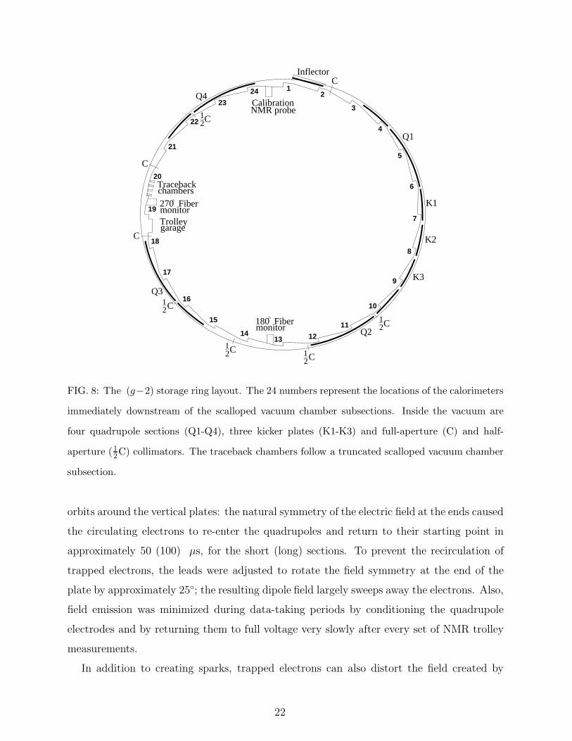
FIG. 8: The (g−2) storage ring layout. The 24 numbers represent the locations of the calorimeters
immediately downstream of the scalloped vacuum chamber subsections. Inside the vacuum are
four quadrupole sections (Q1-Q4), three kicker plates (K1-K3) and full-aperture (C) and half-
aperture (12C) collimators. The traceback chambers follow a truncated scalloped vacuum chamber
subsection.
orbits around the vertical plates: the natural symmetry of the electric field at the ends caused
the circulating electrons to re-enter the quadrupoles and return to their starting point in
approximately 50 (100) µs, for the short (long) sections. To prevent the recirculation of
trapped electrons, the leads were adjusted to rotate the field symmetry at the end of the
plate by approximately 25; the resulting dipole field largely sweeps away the electrons. Also,
field emission was minimized during data-taking periods by conditioning the quadrupole
electrodes and by returning them to full voltage very slowly after every set of NMR trolley
measurements.
In addition to creating sparks, trapped electrons can also distort the field created by
22
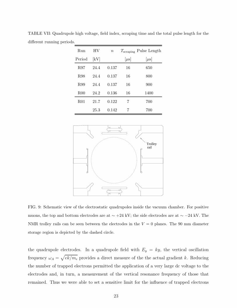
TABLE VII: Quadrupole high voltage, field index, scraping time and the total pulse length for the
different running periods.
Run HV n Tscraping Pulse Length
Period [kV] [µs] [µs]
R97 24.4 0.137 16 650
R98 24.4 0.137 16 800
R99 24.4 0.137 16 900
R00 24.2 0.136 16 1400
R01 21.7 0.122 7 700
25.3 0.142 7 700
Trolleyrail
FIG. 9: Schematic view of the electrostatic quadrupoles inside the vacuum chamber. For positive
muons, the top and bottom electrodes are at ∼ +24 kV; the side electrodes are at ∼ −24 kV. The
NMR trolley rails can be seen between the electrodes in the V = 0 planes. The 90 mm diameter
storage region is depicted by the dashed circle.
the quadrupole electrodes. In a quadrupole field with Ey = ky, the vertical oscillation
frequency ωA =√ek/me provides a direct measure of the the actual gradient k. Reducing
the number of trapped electrons permitted the application of a very large dc voltage to the
electrodes and, in turn, a measurement of the vertical resonance frequency of those that
remained. Thus we were able to set a sensitive limit for the influence of trapped electrons
23
on the electric-field configuration as well as a limit on the magnetic fields that they must
also produce.
F. Pulsed kicker magnet
Direct muon injection requires a pulsed kicker [20] to place the muon bunch into the phase
space acceptance of the storage ring. The center of the circular orbit for muons entering
through the inflector channel is offset from that of the storage ring and, left alone, muons
would strike the inflector exit after one revolution and be lost. A kick of approximately
10 mrad (∼ 0.1 T·m) applied one quarter of a betatron wavelength downstream of the
inflector exit is needed to place the injected bunch on an orbit concentric with the ring
center. The ideal kick would be applied during the first revolution of the bunch and then
turned off before the bunch returns on its next pass.
The E821 kicker makes use of two parallel current sheets with cross-overs at each end
so that the current runs in opposite directions in the two plates. The 80-mm high kicker
plates are 0.75-mm thick aluminum, electron-beam welded to aluminum rails at the top
and bottom, which support the assembly and serve as rails for the 2-kg NMR trolley. The
entire assembly is 94-mm high and 1760-mm long. This plate-rail assembly is supported
on Macorr insulators that are attached to Macorr plates with plastic hardware forming a
rigid cage, which is placed inside of the vacuum chamber. OPERA [21] calculations indicated
that aluminum would minimize the residual eddy currents following the kicker pulse, and
measurements showed that the presence of this aluminum assembly would have a negligible
effect on the storage ring precision magnetic field.
The kicker is energized by an LCR pulse-forming network (PFN), which consists of a
single capacitor, resistor, and the loop formed by the kicker plates. The capacitor is charged
by a resonant circuit and the current pulse is created when the capacitor is shorted to ground
at the firing of a deuterium thyratron. The total inductance of the PFN is L = 1.6 µH,
which effectively limits both the peak current and the minimum achievable pulse width. The
resistance is R = 11.9 Ω and the capacitance is C = 10.1 nF. For the damped LCR circuit,
the oscillation frequency is fd = 1.08× 10⁶ Hz and the decay time is τd = 924 ns. The peak
current is given by I0 = V0/(2πfdL), where V0 is the initial voltage on the capacitor. The
resulting current pulse has a base width of ∼ 400 ns, which is long compared to the 149 ns
24
cyclotron period. Therefore, the positive kick acts on the muon bunch in the first, second,
and third turns of the storage ring.
The kicker consists of three identical sections, each driven by a separate PFN; this division
keeps the inductance of a single assembly at a reasonable value. In each circuit, an initial
voltage of ∼ 90 kV on the capacitor results in a current-pulse amplitude of approximately
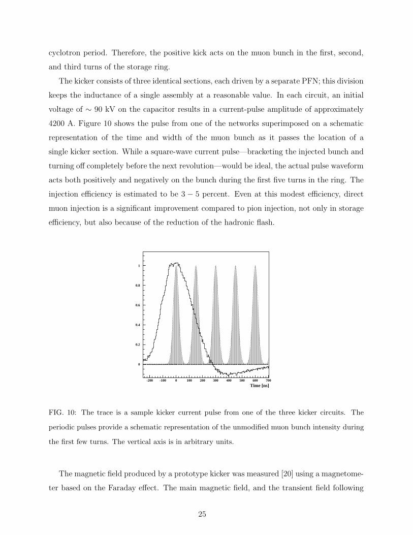
4200 A. Figure 10 shows the pulse from one of the networks superimposed on a schematic
representation of the time and width of the muon bunch as it passes the location of a
single kicker section. While a square-wave current pulse—bracketing the injected bunch and
turning off completely before the next revolution—would be ideal, the actual pulse waveform
acts both positively and negatively on the bunch during the first five turns in the ring. The
injection efficiency is estimated to be 3 − 5 percent. Even at this modest efficiency, direct
muon injection is a significant improvement compared to pion injection, not only in storage
efficiency, but also because of the reduction of the hadronic flash.
Time [ns]
0
0.2
0.4
0.6
0.8
1
-200 -100 0 100 200 300 400 500 600 700
FIG. 10: The trace is a sample kicker current pulse from one of the three kicker circuits. The
periodic pulses provide a schematic representation of the unmodified muon bunch intensity during
the first few turns. The vertical axis is in arbitrary units.
The magnetic field produced by a prototype kicker was measured [20] using a magnetome-
ter based on the Faraday effect. The main magnetic field, and the transient field following
25
s]µTime [-8 -6 -4 -2 0 2 4 6 8 10 12
B [
µT]
-10
-8
-6
-4
-2
0
2
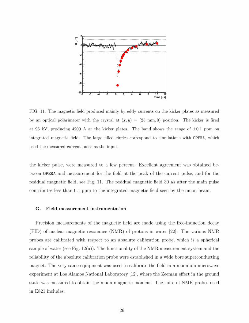
FIG. 11: The magnetic field produced mainly by eddy currents on the kicker plates as measured
by an optical polarimeter with the crystal at (x, y) = (25 mm, 0) position. The kicker is fired
at 95 kV, producing 4200 A at the kicker plates. The band shows the range of ±0.1 ppm on
integrated magnetic field. The large filled circles correspond to simulations with OPERA, which
used the measured current pulse as the input.
the kicker pulse, were measured to a few percent. Excellent agreement was obtained be-
tween OPERA and measurement for the field at the peak of the current pulse, and for the
residual magnetic field, see Fig. 11. The residual magnetic field 30 µs after the main pulse
contributes less than 0.1 ppm to the integrated magnetic field seen by the muon beam.
G. Field measurement instrumentation
Precision measurements of the magnetic field are made using the free-induction decay
(FID) of nuclear magnetic resonance (NMR) of protons in water [22]. The various NMR
probes are calibrated with respect to an absolute calibration probe, which is a spherical
sample of water (see Fig. 12(a)). The functionality of the NMR measurement system and the
reliability of the absolute calibration probe were established in a wide bore superconducting
magnet. The very same equipment was used to calibrate the field in a muonium microwave
experiment at Los Alamos National Laboratory [12], where the Zeeman effect in the ground
state was measured to obtain the muon magnetic moment. The suite of NMR probes used
in E821 includes:
26
• A calibration probe with a spherical water sample (Fig. 12(a)), that provides an ab-
solute calibration between the NMR frequency for a proton in a water sample to that
of a free proton [23]. This calibration probe is employed at a plunging station located
at a region inside the storage ring, where special emphasis was put on achieving high
homogeneity of the field.
• A plunging probe (Fig. 12(b)), which can be inserted into the vacuum in the plunging
station at positions matching those of the trolley probe array. The plunging probe is
used to transfer calibration from the absolute calibration probe to the trolley probes.
• A set of 378 fixed probes placed above and below the storage ring volume in the walls
of the vacuum chamber. These probes have a cylindrical water sample oriented with
its axis along the tangential direction (Fig. 12(c)). They continuously monitor the
field during data taking.
• Seventeen probes mounted inside a trolley that can be pulled through the storage ring
to measure the field (Fig. 13). The probes on board the trolley are identical in design
and shape to the fixed probes (Fig. 12(c)).
Initially the trolley and fixed probes contained a water sample. Over the course of the
experiment, between run periods, the water samples in many of the probes were replaced
with petroleum jelly. The jelly has several advantages over water: low evaporation, favorable
relaxation times at room temperature, a proton NMR signal almost comparable to that from
water, and a chemical shift (and thus the NMR frequency) having a negligible temperature
coefficient.
The free-induction decay signals are obtained after pulsed excitation, using narrow-band
duplexing, multiplexing, and filtering electronics [22]. The signals from all probes are mixed
with a standard frequency fref = 61.74 MHz corresponding to a reference magnetic field
Bref . The reference frequency is obtained from a synthesizer, which is phase-locked to the
base clock of the LORAN C broadcast frequency standard [24], accurate to 10−11. In a
typical probe, the nuclear spins of the water sample are excited by an rf pulse of 5 W and
10 µs length applied to the resonance circuit. The coil Ls and the capacitance Cs form a
resonant circuit at the NMR frequency with a quality factor of typically 100. The coil Lp
serves to match the impedances of the probe assembly and the cable. The rf pulse produces
27
spherical sample holder
1 cm
cable
tuning capacitors
pyrex tubeteflon adaptor
aluminumpure water
teflon holder
copper
.
(a) Absolute calibration probe
copperaluminum
.
teflon
12 mm
ssp
80 mm
L LC
cable
(b) Plunging probe
s
s
p CLcable
aluminum aluminum
100 mm
8 mm
teflon
L 42H O + CuSO.
(c) Trolley and fixed probe
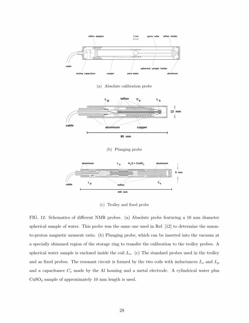
FIG. 12: Schematics of different NMR probes. (a) Absolute probe featuring a 10 mm diameter
spherical sample of water. This probe was the same one used in Ref. [12] to determine the muon-
to-proton magnetic moment ratio. (b) Plunging probe, which can be inserted into the vacuum at
a specially shimmed region of the storage ring to transfer the calibration to the trolley probes. A
spherical water sample is enclosed inside the coil Ls. (c) The standard probes used in the trolley
and as fixed probes. The resonant circuit is formed by the two coils with inductances Ls and Lp
and a capacitance Cs made by the Al housing and a metal electrode. A cylindrical water plus
CuSO4 sample of approximately 10 mm length is used.
28
a linearly polarized rf field ~H in coil Ls, orthogonal to the dipole field. The rf pulse rotates
the macroscopic magnetization in the probe by 90. The NMR signal from the precessing
magnetization at the frequency fNMR is picked up by the coil Ls of the same resonance
circuit and transmitted back through a duplexer to the input of a low-noise preamplifier. It
is then mixed with fref to obtain the intermediate frequency fFID. We set fref smaller than
fNMR for all probes so that fFID is approximately 50 kHz. The typical FID signal decays
exponentially and the time between the first and last zero crossing—the latter defined by
when the amplitude has decayed to about 1/3 of its initial value [22]—is of order 1 ms.
The interval is measured with a resolution of 50 ns and the number of crossings in this
interval is counted. The ratio gives the frequency fFID for a single measurement, which can
be converted to the magnetic field Breal at the location of the probe’s active volume through
the relation
Breal = Bref
(1 +
Breal − Bref
Bref
)= Bref
(1 +
fFID
fref
). (13)
The analysis procedure, which is used to determine the average magnetic field from the raw
NMR data, is discussed in Section IVA.
H. Detector systems, electronics and data acquisition
1. Electromagnetic calorimeters
Twenty-four electromagnetic calorimeters are placed symmetrically around the inside of
the storage ring, adjacent to the vacuum chamber, which has a scalloped shape to permit
decay electrons to exit the vacuum through a flat face cutout upstream of each calorimeter
(see Fig. 8). The calorimeters are used to measure the decay electron energy and time of
arrival. They are constrained in height by the magnet yoke gap. The width and depth were
chosen to optimize the acceptance for high-energy electrons, and minimize the low-energy
electron acceptance. Each calorimeter is 140 mm high by 230 mm wide and has a depth
of 13 radiation lengths (150 mm). The 24 calorimeters intercept approximately 65 percent
of the electrons having energy greater than 1.8 GeV. The acceptance falls with decreasing
electron energy.
Because of the high rate (few MHz) at early times following injection,fast readout and
excellent pulse separation (in time) are necessary characteristics of the design. They are
29
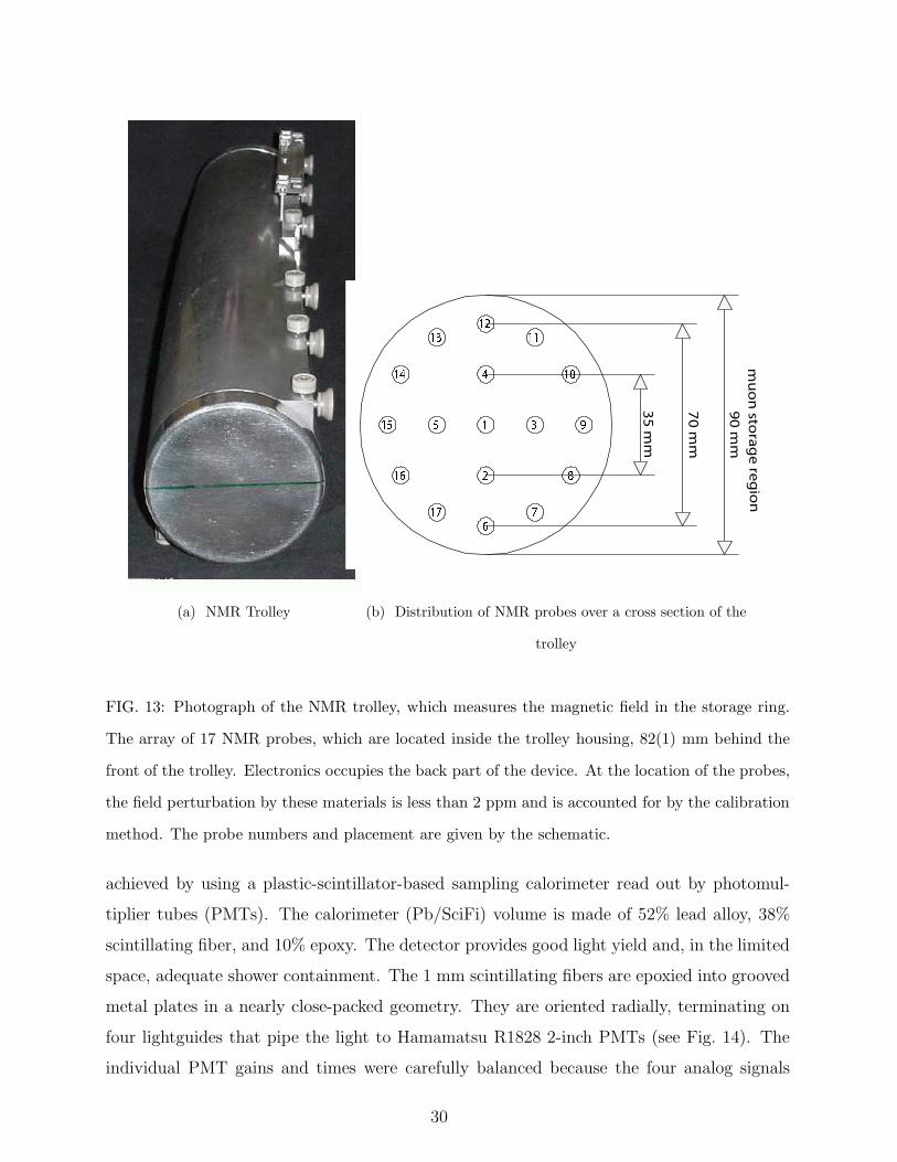
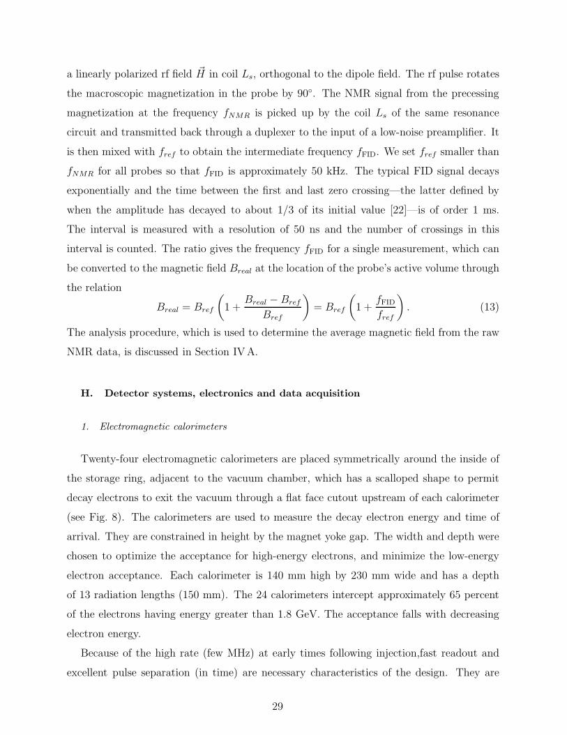
(a) NMR Trolley (b) Distribution of NMR probes over a cross section of the
trolley
FIG. 13: Photograph of the NMR trolley, which measures the magnetic field in the storage ring.
The array of 17 NMR probes, which are located inside the trolley housing, 82(1) mm behind the
front of the trolley. Electronics occupies the back part of the device. At the location of the probes,
the field perturbation by these materials is less than 2 ppm and is accounted for by the calibration
method. The probe numbers and placement are given by the schematic.
achieved by using a plastic-scintillator-based sampling calorimeter read out by photomul-
tiplier tubes (PMTs). The calorimeter (Pb/SciFi) volume is made of 52% lead alloy, 38%
scintillating fiber, and 10% epoxy. The detector provides good light yield and, in the limited
space, adequate shower containment. The 1 mm scintillating fibers are epoxied into grooved
metal plates in a nearly close-packed geometry. They are oriented radially, terminating on
four lightguides that pipe the light to Hamamatsu R1828 2-inch PMTs (see Fig. 14). The
individual PMT gains and times were carefully balanced because the four analog signals
30
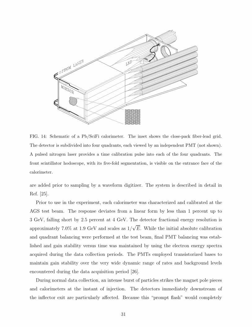
FIG. 14: Schematic of a Pb/SciFi calorimeter. The inset shows the close-pack fiber-lead grid.
The detector is subdivided into four quadrants, each viewed by an independent PMT (not shown).
A pulsed nitrogen laser provides a time calibration pulse into each of the four quadrants. The
front scintillator hodoscope, with its five-fold segmentation, is visible on the entrance face of the
calorimeter.
are added prior to sampling by a waveform digitizer. The system is described in detail in
Ref. [25].
Prior to use in the experiment, each calorimeter was characterized and calibrated at the
AGS test beam. The response deviates from a linear form by less than 1 percent up to
3 GeV, falling short by 2.5 percent at 4 GeV. The detector fractional energy resolution is
approximately 7.0% at 1.9 GeV and scales as 1/√E. While the initial absolute calibration
and quadrant balancing were performed at the test beam, final PMT balancing was estab-
lished and gain stability versus time was maintained by using the electron energy spectra
acquired during the data collection periods. The PMTs employed transistorized bases to
maintain gain stability over the very wide dynamic range of rates and background levels
encountered during the data acquisition period [26].
During normal data collection, an intense burst of particles strikes the magnet pole pieces
and calorimeters at the instant of injection. The detectors immediately downstream of
the inflector exit are particularly affected. Because this “prompt flash” would completely
31
saturate the PMTs, they are gated off prior to injection and turned back on some tens of
microseconds later, depending on the location of the calorimeter with respect to the inflector
exit. The output of a PMT was suppressed by a factor of 106 by exchanging the bias on
dynodes 4 and 7. When the dynodes are reset, the gain returned to better than 99 percent
of its steady-state value in approximately 1 µs.
The prompt flash creates an enormous number of neutrons, many of which are thermalized
and captured inside the Pb/SciFi calorimeters. Capture gamma rays can knock out electrons,
which traverse the scintillating fibers. The generated light gives an elevated background
pedestal that diminishes with the time dependence: ≈ t−1.3 for t > 5 µs. The effective decay
time was minimized by doping detectors in the first half of the ring—where the capture rate
is highest—with a natural boron carbide powder. The 10B component (20 percent) has a
high thermal-neutron capture cross section.
To monitor the detectors, a 300 ps uv (λ = 337 nm) pulse from a nitrogen laser is di-
rected through a splitter system into an outside radial corner of each of the quadrants of
all calorimeters. The uv pulse is absorbed by a sample of scintillating fibers. These fibers
promptly emit a light pulse having the same fluorescence spectrum as produced by a passing
charged particle. The calibration pulse propagates through the entire optical and electronic
readout system. A reference photodiode and PMT—located well outside the storage ring—
also receive a fixed fraction of the light from the laser pulse. The laser was fired every other
fill, in parallel with the beam data, during 20-minute runs scheduled once per 8-hour shift.
Firings alternated among four points in time with respect to beam injection. These points
were changed for each laser run, providing a map of any possible gain or timing changes.
Timing shifts were found to be limited to less than 4 ps from early-to-late times, corre-
sponding to an upper limit of 0.02 ppm systematic uncertainty in ωa. No overall trends were
seen in the laser-based gain change data. Observed gain changes were generally a few tenths
of a percent, without a preferred sign. Unfortunately, the scatter in the these calibration
measurements is much greater than is allowed by statistics, and the mechanism responsible
has not been identified. Consequently, the laser-based gain stability (see Section IVB2)
could be established to no better than a few tenths of a percent. Ultimately, monitoring the
endpoints of the electron energy spectra provided a better measurement of gain stability.
32
2. Special detector systems
Hodoscopes consisting of five horizontal bars of scintillator—the front scintillating detec-
tors (FSDs)—are attached to the front face of the calorimeters (Fig. 14). The FSDs are
used to measure the rate of “lost muons” from the storage ring and to provide a vertical
profile of electrons on the front face of the calorimeters. The FSD signals are also used as
a check on the pulse times reconstructed from the calorimeter waveforms. The individual
scintillators are 235 mm long (radial), 28 mm high and 10 mm thick. They are coupled
adiabatically to 28-mm diameter Hamamatsu R6427 PMTs, located below the storage ring
magnet midplane. The PMT bases are gated off at injection, following a scheme similar to
that used in the calorimeter PMT bases. (Eventually, over the run periods, about half of the
FSD stations were instrumented with PMTs.) An FSD signal is recognized by a leading-edge
discriminator and is recorded by a multi-hit time-to-digital converter (MTDC).
An xy hodoscope with 7 mm segmentation is mounted on the front face of five calorime-
ters. These position-sensitive detectors (PSDs) have 20 horizontal and 32 vertical scintillator
sticks read out by wavelength-shifting fibers and a Philips multi-anode phototube (later re-
placed by a multi-channel DEP hybrid photodiode). The MTDC recorded event time and
custom electronics coded the xy profile, providing information on albedo and multiplicity
versus time. In some cases, a calorimeter was equipped with both PSD and FSD, providing
efficiency checks of each. The vertical profiles of both FSD and PSD provide sensitivity to
the presence of an electric dipole moment, which would tilt the precession plane of the muon
spin.
Depending on the average AGS intensity for each running period, either a thin scintillator
or Cerenkov counter is located in the beamline, just outside the muon storage ring. This
“T0” counter records the arrival time and intensity (time) profile of a muon bunch from the
AGS. Injected pulses not exceeding a set integrated current in T0 are rejected in the offline
analysis because they do not provide a good reference start time for the fill and because
they are generally associated with bad AGS extraction.
Scintillating-fiber beam-monitors (FBM), which are rotated into the storage region under
vacuum, were used to observe directly the beam motion in the storage ring during special
systematic study runs. Separate FBMs measure the horizontal and vertical beam distribu-
tions. Each FBM is composed of seven fibers centered within the muon storage region to
33
±0.5 mm. The 90-mm long fibers are separated by 13 mm. One end is mated to a clear
fiber, which carries the light out of the vacuum chamber to PMTs mounted on top of the
storage ring magnet. The PMTs are sampled continuously for about 10 µs using 200 MHz
waveform digitizers. The beam lifetime with the fiber beam monitors in the storage region
is about one half the 64 µs muon decay lifetime.
The scalloped vacuum chamber is truncated at one location and a 360 µm-thick mylar
window (72 mm wide by 110 mm high) replaces the aluminum flat exit face to allow electrons
to pass through a minimum of scattering material. A set of four rectangular drift chambers—
the traceback system [27]—is positioned between this window and calorimeter station #20.
Each chamber consists of three layers of 8-mm diameter straw drift tubes oriented vertically
and radially. An electron that exits the window and passes through the four chambers
is tracked by up to 12 vertical and 12 radial measurements. Although decay electrons
are not always emitted tangentially, their radial momenta are sufficiently small so that an
extrapolation of the track back to the point of tangency with the central muon orbit yields
a measurement of the actual muon decay position, as well as its vertical decay angle. The
former is helpful in establishing the average positions and therefore the average field felt by
the muons.
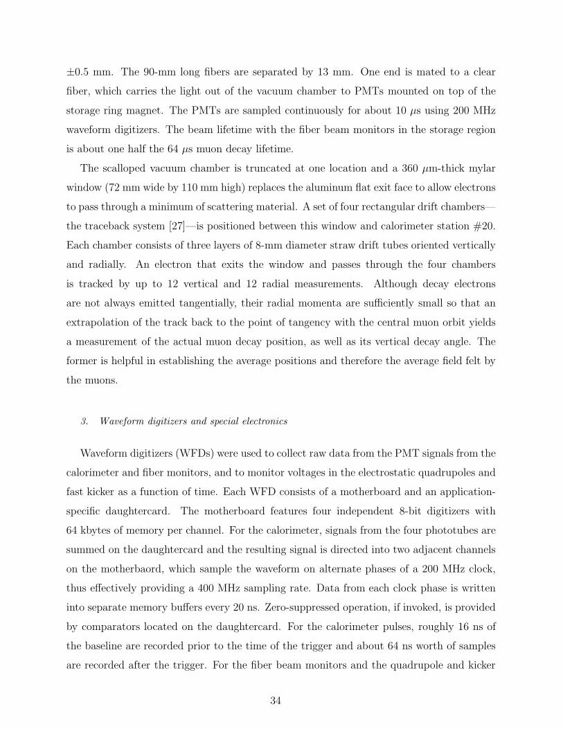
3. Waveform digitizers and special electronics
Waveform digitizers (WFDs) were used to collect raw data from the PMT signals from the
calorimeter and fiber monitors, and to monitor voltages in the electrostatic quadrupoles and
fast kicker as a function of time. Each WFD consists of a motherboard and an application-
specific daughtercard. The motherboard features four independent 8-bit digitizers with
64 kbytes of memory per channel. For the calorimeter, signals from the four phototubes are
summed on the daughtercard and the resulting signal is directed into two adjacent channels
on the motherbaord, which sample the waveform on alternate phases of a 200 MHz clock,
thus effectively providing a 400 MHz sampling rate. Data from each clock phase is written
into separate memory buffers every 20 ns. Zero-suppressed operation, if invoked, is provided
by comparators located on the daughtercard. For the calorimeter pulses, roughly 16 ns of
the baseline are recorded prior to the time of the trigger and about 64 ns worth of samples
are recorded after the trigger. For the fiber beam monitors and the quadrupole and kicker
34
Time (ns)0 10 20 30 40 50 60 70 80
Pu
lse
hei
gh
t (A
DC
un
its)
0
20
40
60
80
100
120
140
160
Time (ns)0 10 20 30 40 50 60 70 80
Pu
lse
hei
gh
t (A
DC
un
its)
0
20
40
60
80
100
120
140
FIG. 15: Examples of waveform digitizer samples from a calorimeter. The two WFD phases are
alternately shaded. The left panel shows a simple, single pulse, while the right panel has two
overlapping pulses separated by 7.5 ns.
voltage readout, four different versions of the daughtercards were used. Sampling rates
varied: 200 MHz for the fiber monitors and kicker, 2 MHz for the quad voltage monitor.
These WFDs were operated without zero suppression.
The time words written to memory in each of the two phases have a fixed but arbitrary
offset in any data-collection cycle. To resolve the ambiguity, a 150 ns triangular pulse is
directed into a fifth analog input on each daughtercard immediately prior to each fill. By
reconstructing this “marker pulse,” the unknown offset is determined unambiguously, and
the data streams can then be combined in the offline reconstruction program. Typical
calorimeter pulses, with samples from the two phases interleaved, are shown in Fig. 15.
The clock signals for the WFD, MTDC and NMR are all derived from the same frequency
synthesizer, which is synchronized to the Loran C time standard [24]. There is no correlation
between the experiment clock and the AGS clock that determines the time of injection. This
effectively randomizes the electronic sampling times relative to the injection times at the
∼ 5 ns time scale, greatly reducing possible systematic errors associated with odd-even
effects in the WFDs.
35
III. BEAM DYNAMICS
A. Overview
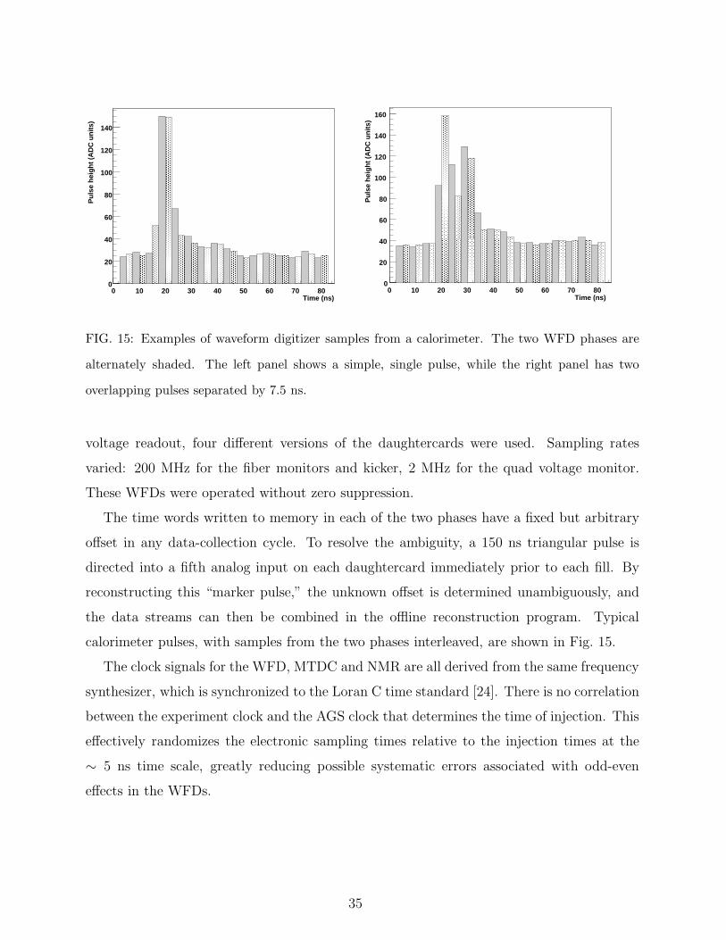
The muon storage ring uses the electrostatic quadrupoles to obtain weak vertical fo-
cussing [28, 29]. The field index is given by:
n =R0
vB0
∂Ey
∂y, (14)
where R0 is the central orbit radius, B0 is the dipole magnetic field, and v is the muon
speed. The coordinate system is shown in Fig. 16. High voltage of ±24 kV applied to the
quadrupole plates gives an n value of 0.137, which is the field index that was used in the
R97-99 periods. The R00 period used n = 0.135 and the R01 running was split into “low-”
and “high-n” sub-periods with n = 0.122 and 0.142, respectively. The field index value
determines the stored muon beam betatron motion, which in turn can perturb the electron
time distribution, as discussed in Section IIIC.
For an ideal weak-focusing ring, where the quadrupole field is constant in time and
uniform in azimuth, the horizontal and vertical tunes are given by νx =√
(1 − n) and
νy =√n. Consider the motion of a particular muon having momentum p compared to the
magic momentum p0. Its horizontal and vertical betatron oscillations are described by
x = xe + Ax cos(νxφ+ φ0x) (15)
y = Ay cos(νyφ+ φ0y). (16)
Here φ = s/R0, where s is the azimuthal distance around the ring and Ax and Ay are
amplitudes of the oscillations about the equilibrium orbit (xe) and the horizontal midplane,
respectively, with xe given by
xe = R0
(p− p0
p0(1 − n)
). (17)
The maximum accepted horizontal and vertical angles are defined by the 45 mm radius of
the storage volume, rmax, giving
θhmax =
rmax
√1 − n
R0
(18)
θvmax =
rmax
√n
R0. (19)
36
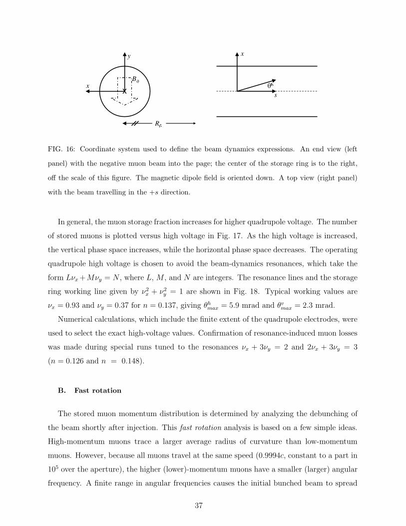
FIG. 16: Coordinate system used to define the beam dynamics expressions. An end view (left
panel) with the negative muon beam into the page; the center of the storage ring is to the right,
off the scale of this figure. The magnetic dipole field is oriented down. A top view (right panel)
with the beam travelling in the +s direction.
In general, the muon storage fraction increases for higher quadrupole voltage. The number
of stored muons is plotted versus high voltage in Fig. 17. As the high voltage is increased,
the vertical phase space increases, while the horizontal phase space decreases. The operating
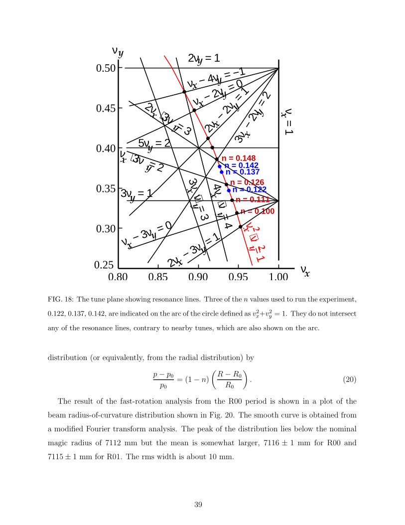
quadrupole high voltage is chosen to avoid the beam-dynamics resonances, which take the
form Lνx +Mνy = N , where L, M , and N are integers. The resonance lines and the storage
ring working line given by ν2x + ν2
y = 1 are shown in Fig. 18. Typical working values are
νx = 0.93 and νy = 0.37 for n = 0.137, giving θhmax = 5.9 mrad and θv
max = 2.3 mrad.
Numerical calculations, which include the finite extent of the quadrupole electrodes, were
used to select the exact high-voltage values. Confirmation of resonance-induced muon losses
was made during special runs tuned to the resonances νx + 3νy = 2 and 2νx + 3νy = 3
(n = 0.126 and n = 0.148).
B. Fast rotation
The stored muon momentum distribution is determined by analyzing the debunching of
the beam shortly after injection. This fast rotation analysis is based on a few simple ideas.
High-momentum muons trace a larger average radius of curvature than low-momentum
muons. However, because all muons travel at the same speed (0.9994c, constant to a part in
105 over the aperture), the higher (lower)-momentum muons have a smaller (larger) angular
frequency. A finite range in angular frequencies causes the initial bunched beam to spread
37
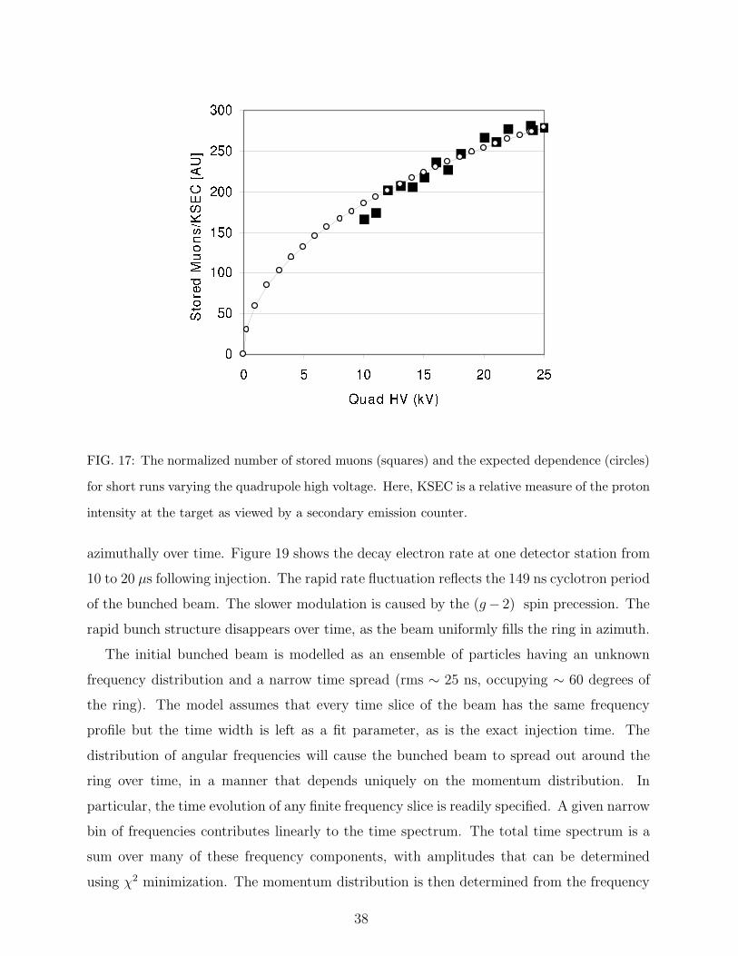
FIG. 17: The normalized number of stored muons (squares) and the expected dependence (circles)
for short runs varying the quadrupole high voltage. Here, KSEC is a relative measure of the proton
intensity at the target as viewed by a secondary emission counter.
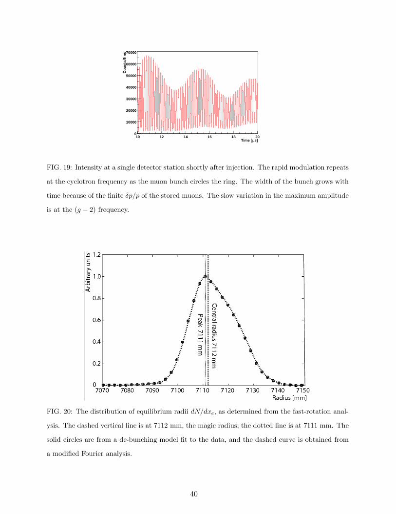
azimuthally over time. Figure 19 shows the decay electron rate at one detector station from
10 to 20 µs following injection. The rapid rate fluctuation reflects the 149 ns cyclotron period
of the bunched beam. The slower modulation is caused by the (g− 2) spin precession. The
rapid bunch structure disappears over time, as the beam uniformly fills the ring in azimuth.
The initial bunched beam is modelled as an ensemble of particles having an unknown
frequency distribution and a narrow time spread (rms ∼ 25 ns, occupying ∼ 60 degrees of
the ring). The model assumes that every time slice of the beam has the same frequency
profile but the time width is left as a fit parameter, as is the exact injection time. The
distribution of angular frequencies will cause the bunched beam to spread out around the
ring over time, in a manner that depends uniquely on the momentum distribution. In
particular, the time evolution of any finite frequency slice is readily specified. A given narrow
bin of frequencies contributes linearly to the time spectrum. The total time spectrum is a
sum over many of these frequency components, with amplitudes that can be determined
using χ2 minimization. The momentum distribution is then determined from the frequency
38
n = 0.100
xy
2ν = 1y
2ν −
2ν =
1
x
y3ν
− 2ν
= 2
xy
ν − 2ν = 0
xy
3ν +ν = 3x
y
4ν + ν = 4x
y
ν = 1x
5ν = 2y
3ν = 1y
ν − 3ν = 0
xy
2ν − 3ν = 1
x
y
xy
ν + 3ν = 2
xy
2ν + 3ν = 3
xy
22
ν + ν = 1
0.90 0.95 1.000.850.25
0.80
0.50
0.30
0.35
0.40
0.45
ν
νx
y
n = 0.142n = 0.148
n = 0.126n = 0.137
n = 0.111n = 0.122
ν − 4ν = −1
FIG. 18: The tune plane showing resonance lines. Three of the n values used to run the experiment,
0.122, 0.137, 0.142, are indicated on the arc of the circle defined as v2x+v2
y = 1. They do not intersect
any of the resonance lines, contrary to nearby tunes, which are also shown on the arc.
distribution (or equivalently, from the radial distribution) by
p− p0
p0= (1 − n)
(R −R0
R0
). (20)
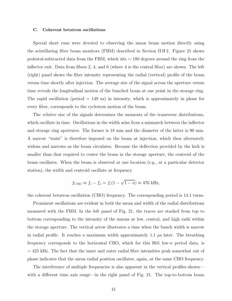
The result of the fast-rotation analysis from the R00 period is shown in a plot of the
beam radius-of-curvature distribution shown in Fig. 20. The smooth curve is obtained from
a modified Fourier transform analysis. The peak of the distribution lies below the nominal
magic radius of 7112 mm but the mean is somewhat larger, 7116 ± 1 mm for R00 and
7115 ± 1 mm for R01. The rms width is about 10 mm.
39
s]µTime [10 12 14 16 18 20
Co
un
ts/5
ns
0
10000
20000
30000
40000
50000
60000
70000
FIG. 19: Intensity at a single detector station shortly after injection. The rapid modulation repeats
at the cyclotron frequency as the muon bunch circles the ring. The width of the bunch grows with
time because of the finite δp/p of the stored muons. The slow variation in the maximum amplitude
is at the (g − 2) frequency.
FIG. 20: The distribution of equilibrium radii dN/dxe, as determined from the fast-rotation anal-
ysis. The dashed vertical line is at 7112 mm, the magic radius; the dotted line is at 7111 mm. The
solid circles are from a de-bunching model fit to the data, and the dashed curve is obtained from
a modified Fourier analysis.
40
C. Coherent betatron oscillations
Special short runs were devoted to observing the muon beam motion directly using
the scintillating fiber beam monitors (FBM) described in Section IIH 2. Figure 21 shows
pedestal-subtracted data from the FBM, which sits ∼ 180 degrees around the ring from the
inflector exit. Data from fibers 2, 4, and 6 (where 4 is the central fiber) are shown. The left
(right) panel shows the fiber intensity representing the radial (vertical) profile of the beam
versus time shortly after injection. The average size of the signal across the aperture versus
time reveals the longitudinal motion of the bunched beam at one point in the storage ring.
The rapid oscillation (period = 149 ns) in intensity, which is approximately in phase for
every fiber, corresponds to the cyclotron motion of the beam.
The relative size of the signals determines the moments of the transverse distributions,
which oscillate in time. Oscillations in the width arise from a mismatch between the inflector
and storage ring apertures. The former is 18 mm and the diameter of the latter is 90 mm.
A narrow “waist” is therefore imposed on the beam at injection, which then alternately
widens and narrows as the beam circulates. Because the deflection provided by the kick is
smaller than that required to center the beam in the storage aperture, the centroid of the
beam oscillates. When the beam is observed at one location (e.g., at a particular detector
station), the width and centroid oscillate at frequency
fCBO ≈ fc − fx = fc(1 −√
1 − n) ≈ 476 kHz,
the coherent betatron oscillation (CBO) frequency. The corresponding period is 14.1 turns.
Prominent oscillations are evident in both the mean and width of the radial distributions
measured with the FBM. In the left panel of Fig. 21, the traces are stacked from top to
bottom corresponding to the intensity of the muons at low, central, and high radii within
the storage aperture. The vertical arrow illustrates a time when the bunch width is narrow
in radial profile. It reaches a maximum width approximately 1.1 µs later. The breathing
frequency corresponds to the horizontal CBO, which for this R01 low-n period data, is
∼ 425 kHz. The fact that the inner and outer radial fiber intensities peak somewhat out of
phase indicates that the mean radial position oscillates, again, at the same CBO frequency.
The interference of multiple frequencies is also apparent in the vertical profiles shown—
with a different time axis range—in the right panel of Fig. 21. The top-to-bottom beam
41
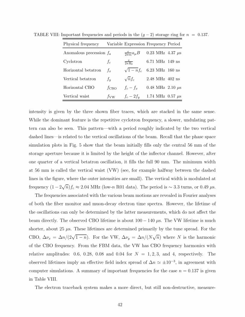
TABLE VIII: Important frequencies and periods in the (g − 2) storage ring for n = 0.137.
Physical frequency Variable Expression Frequency Period
Anomalous precession fae
2πmaµB 0.23 MHz 4.37 µs
Cyclotron fcv
2πR06.71 MHz 149 ns
Horizontal betatron fx
√1 − nfc 6.23 MHz 160 ns
Vertical betatron fy√
nfc 2.48 MHz 402 ns
Horizontal CBO fCBO fc − fx 0.48 MHz 2.10 µs
Vertical waist fVW fc − 2fy 1.74 MHz 0.57 µs
intensity is given by the three shown fiber traces, which are stacked in the same sense.
While the dominant feature is the repetitive cyclotron frequency, a slower, undulating pat-
tern can also be seen. This pattern—with a period roughly indicated by the two vertical
dashed lines—is related to the vertical oscillations of the beam. Recall that the phase space
simulation plots in Fig. 5 show that the beam initially fills only the central 56 mm of the
storage aperture because it is limited by the height of the inflector channel. However, after
one quarter of a vertical betatron oscillation, it fills the full 90 mm. The minimum width
at 56 mm is called the vertical waist (VW) (see, for example halfway between the dashed
lines in the figure, where the outer intensities are small). The vertical width is modulated at
frequency (1−2√n)fc ≈ 2.04 MHz (low-n R01 data). The period is ∼ 3.3 turns, or 0.49 µs.
The frequencies associated with the various beam motions are revealed in Fourier analyses
of both the fiber monitor and muon-decay electron time spectra. However, the lifetime of
the oscillations can only be determined by the latter measurements, which do not affect the
beam directly. The observed CBO lifetime is about 100− 140 µs. The VW lifetime is much
shorter, about 25 µs. These lifetimes are determined primarily by the tune spread. For the
CBO, ∆νx = ∆n/(2√
1 − n). For the VW, ∆νy = ∆n/(N√n) where N is the harmonic
of the CBO frequency. From the FBM data, the VW has CBO frequency harmonics with
relative amplitudes: 0.6, 0.28, 0.08 and 0.04 for N = 1, 2, 3, and 4, respectively. The
observed lifetimes imply an effective field index spread of ∆n ≃ ±10−3, in agreement with
computer simulations. A summary of important frequencies for the case n = 0.137 is given
in Table VIII.
The electron traceback system makes a more direct, but still non-destructive, measure-
42
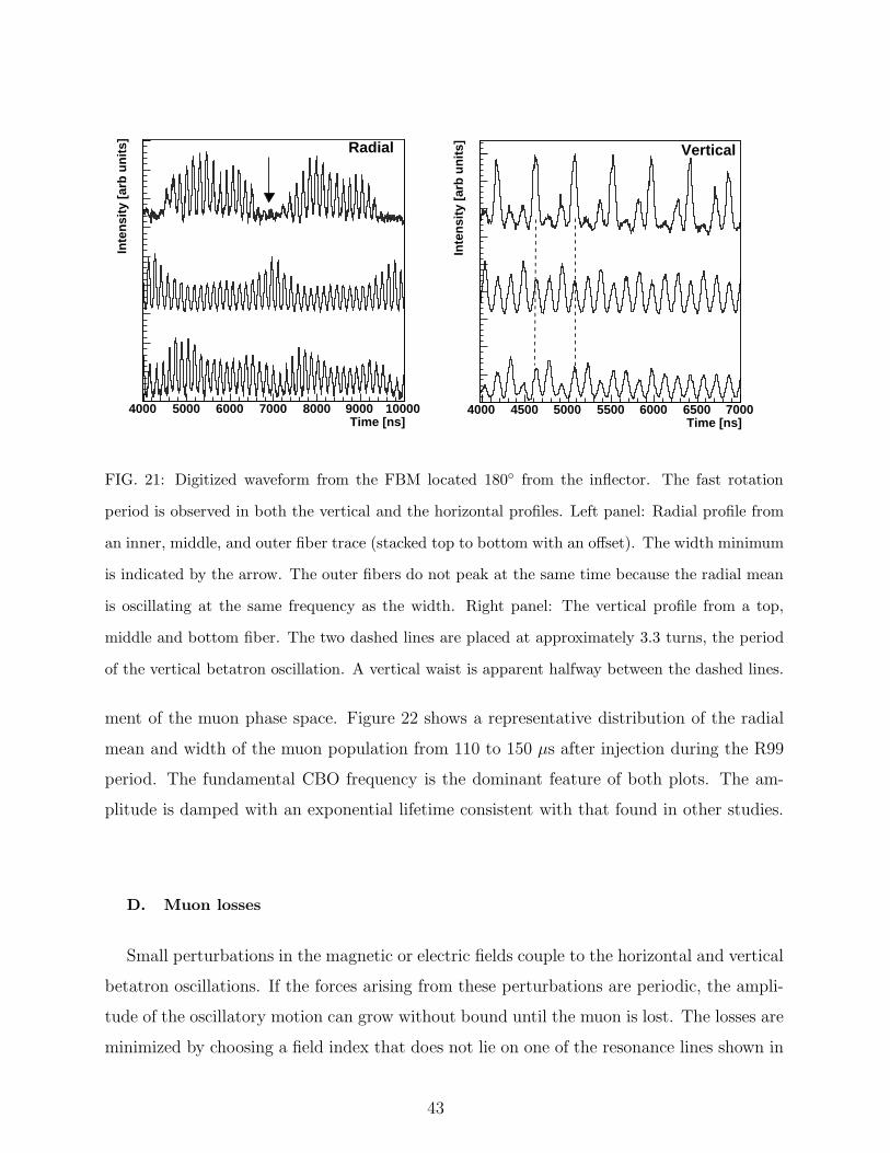
Time [ns]4000 5000 6000 7000 8000 9000 10000
Inte
nsi
ty [
arb
un
its] Radial
Time [ns]4000 4500 5000 5500 6000 6500 7000
Inte
nsi
ty [
arb
un
its] Vertical
FIG. 21: Digitized waveform from the FBM located 180 from the inflector. The fast rotation
period is observed in both the vertical and the horizontal profiles. Left panel: Radial profile from
an inner, middle, and outer fiber trace (stacked top to bottom with an offset). The width minimum
is indicated by the arrow. The outer fibers do not peak at the same time because the radial mean
is oscillating at the same frequency as the width. Right panel: The vertical profile from a top,
middle and bottom fiber. The two dashed lines are placed at approximately 3.3 turns, the period
of the vertical betatron oscillation. A vertical waist is apparent halfway between the dashed lines.
ment of the muon phase space. Figure 22 shows a representative distribution of the radial
mean and width of the muon population from 110 to 150 µs after injection during the R99
period. The fundamental CBO frequency is the dominant feature of both plots. The am-
plitude is damped with an exponential lifetime consistent with that found in other studies.
D. Muon losses
Small perturbations in the magnetic or electric fields couple to the horizontal and vertical
betatron oscillations. If the forces arising from these perturbations are periodic, the ampli-
tude of the oscillatory motion can grow without bound until the muon is lost. The losses are
minimized by choosing a field index that does not lie on one of the resonance lines shown in
43
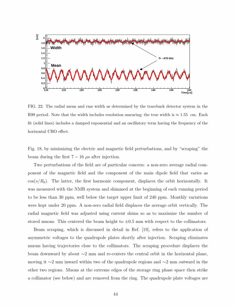
Time 110 115 120 125 130 135 140 145 150
[cm
]
0
0.2
0.4
0.6
0.8
1
1.2
1.4
1.6
1.8
2
Width
Mean
s]µ[
f= ~470 kHz
FIG. 22: The radial mean and rms width as determined by the traceback detector system in the
R99 period. Note that the width includes resolution smearing; the true width is ≈ 1.55 cm. Each
fit (solid lines) includes a damped exponential and an oscillatory term having the frequency of the
horizontal CBO effect.
Fig. 18, by minimizing the electric and magnetic field perturbations, and by “scraping” the
beam during the first 7 − 16 µs after injection.
Two perturbations of the field are of particular concern: a non-zero average radial com-
ponent of the magnetic field and the component of the main dipole field that varies as
cos(s/R0). The latter, the first harmonic component, displaces the orbit horizontally. It
was measured with the NMR system and shimmed at the beginning of each running period
to be less than 30 ppm, well below the target upper limit of 240 ppm. Monthly variations
were kept under 20 ppm. A non-zero radial field displaces the average orbit vertically. The
radial magnetic field was adjusted using current shims so as to maximize the number of
stored muons. This centered the beam height to ±0.5 mm with respect to the collimators.
Beam scraping, which is discussed in detail in Ref. [19], refers to the application of
asymmetric voltages to the quadrupole plates shortly after injection. Scraping eliminates
muons having trajectories close to the collimators. The scraping procedure displaces the
beam downward by about ∼2 mm and re-centers the central orbit in the horizontal plane,
moving it ∼2 mm inward within two of the quadrupole regions and ∼2 mm outward in the
other two regions. Muons at the extreme edges of the storage ring phase space then strike
a collimator (see below) and are removed from the ring. The quadrupole plate voltages are
44
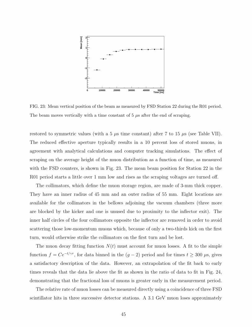
Time [ns]0 10000 20000 30000 40000 50000
Mea
n [
mm
]-2
-1
0
1
2
FIG. 23: Mean vertical position of the beam as measured by FSD Station 22 during the R01 period.
The beam moves vertically with a time constant of 5 µs after the end of scraping.
restored to symmetric values (with a 5 µs time constant) after 7 to 15 µs (see Table VII).
The reduced effective aperture typically results in a 10 percent loss of stored muons, in
agreement with analytical calculations and computer tracking simulations. The effect of
scraping on the average height of the muon distribution as a function of time, as measured
with the FSD counters, is shown in Fig. 23. The mean beam position for Station 22 in the
R01 period starts a little over 1 mm low and rises as the scraping voltages are turned off.
The collimators, which define the muon storage region, are made of 3-mm thick copper.
They have an inner radius of 45 mm and an outer radius of 55 mm. Eight locations are
available for the collimators in the bellows adjoining the vacuum chambers (three more
are blocked by the kicker and one is unused due to proximity to the inflector exit). The
inner half circles of the four collimators opposite the inflector are removed in order to avoid
scattering those low-momentum muons which, because of only a two-thirds kick on the first
turn, would otherwise strike the collimators on the first turn and be lost.
The muon decay fitting function N(t) must account for muon losses. A fit to the simple
function f = Ce−t/γτ , for data binned in the (g − 2) period and for times t ≥ 300 µs, gives
a satisfactory description of the data. However, an extrapolation of the fit back to early
times reveals that the data lie above the fit as shown in the ratio of data to fit in Fig. 24,
demonstrating that the fractional loss of muons is greater early in the measurement period.
The relative rate of muon losses can be measured directly using a coincidence of three FSD
scintillator hits in three successive detector stations. A 3.1 GeV muon loses approximately
45
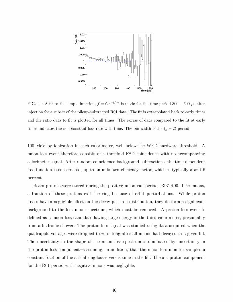
Time [ µs]100 200 300 400 500 600
Dat
a / F
it
0.985
0.99
0.995
1
1.005
1.01
1.015
1.02
FIG. 24: A fit to the simple function, f = Ce−t/γτ is made for the time period 300 − 600 µs after
injection for a subset of the pileup-subtracted R01 data. The fit is extrapolated back to early times
and the ratio data to fit is plotted for all times. The excess of data compared to the fit at early
times indicates the non-constant loss rate with time. The bin width is the (g − 2) period.
100 MeV by ionization in each calorimeter, well below the WFD hardware threshold. A
muon loss event therefore consists of a threefold FSD coincidence with no accompanying
calorimeter signal. After random-coincidence background subtractions, the time-dependent
loss function is constructed, up to an unknown efficiency factor, which is typically about 6
percent.
Beam protons were stored during the positive muon run periods R97-R00. Like muons,
a fraction of these protons exit the ring because of orbit perturbations. While proton
losses have a negligible effect on the decay positron distribution, they do form a significant
background to the lost muon spectrum, which must be removed. A proton loss event is
defined as a muon loss candidate having large energy in the third calorimeter, presumably
from a hadronic shower. The proton loss signal was studied using data acquired when the
quadrupole voltages were dropped to zero, long after all muons had decayed in a given fill.
The uncertainty in the shape of the muon loss spectrum is dominated by uncertainty in
the proton-loss component—assuming, in addition, that the muon-loss monitor samples a
constant fraction of the actual ring losses versus time in the fill. The antiproton component
for the R01 period with negative muons was negligible.
46
E. Electric-field and pitch correction
The magnetic field is adjusted so that the magic momentum p0 (see Eq. 5) is at the center
of the aperture. The (g − 2) precession ωa of muons at this radius is not affected by the
electric field, which is, in any case, zero at the center of the quadrupoles. However, muons of
higher or lower momentum are subject to a linearly rising field and deviate from the magic
momentum, so their (g − 2) frequency is reduced. We apply a correction for this effect. As
the muons oscillate about their equilibrium radii xe, they experience a mean radial electric
field 〈Er〉 = n(βB0/R0)xe. Differentiating Eq. 5 with respect to p, and averaging over the
muon ensemble gives ⟨δωa
ωa
⟩= −2β2n(1 − n)
⟨(xe
Ro
)2⟩
(21)
where 〈x2e〉 is obtained from the fast rotation analysis. While the radial distribution un-
certainty is based on data, it is checked against the simulation. Both methods agree on
the mean-square width to a precision of 5 percent. This uncertainty is added in quadra-
ture with the uncertainty in the mean muon radial position with respect to the electro-
static quadrupoles δR = ±0.5 mm (±0.01 ppm in aµ), and with the uncertainty in the
mean vertical position of the beam ±1 mm (±0.02 ppm in aµ). As a quantitative exam-
ple, the R01 electric-field correction to the precession frequency for the low-n subperiod is
(+0.47±0.05) ppm.
The pitch correction [30] accounts for the fact that vertical betatron motion decreases
slightly the magnetic field felt by the stored muons in their rest frame. When the orbit
is inclined at angle ψ to the horizontal, to sufficient accuracy ωa is reduced by the factor
(1 − 12ψ2). If ψm is the angular amplitude of the vertical oscillation, the average over the
ensemble of muons is (1 − 14〈ψ2
m〉). Here 〈ψ2m〉 = n〈y2〉/R2
0, where 〈y2〉 is the mean-squared
vertical spread of the stored muons, which was measured by the traceback system, confirming
results from the tracking simulation.
The correction to the measured ωa due to vertical betatron oscillations is calculated
for each n value setting. The systematic error is estimated as the difference between the
correction calculated from the simulated and measured muon distributions (±0.03 ppm)
added in quadrature with the uncertainty in the mean muon radial position with respect to
the electrostatic quadrupoles and the uncertainty in the mean vertical position of the beam.
47
For the R01 low-n sub-period, the correction is (+0.27±0.04) ppm.
A tracking program, simulating the muon spin precession in the storage ring—including
the correct azimuthal quadrupole electric field, confirmed the validity of the analytic electric-
field and pitch corrections. The equations given in Ref. [31] were used for the orbit and the
spin motion. The validity of the electric-field and pitch-correction expressions are verified
to 0.01 ppm in aµ .
IV. DATA ANALYSIS
The calculation of aµ requires the determination of the muon spin precession frequency,
ωa, and the average magnetic field seen by the muons, ωp. “Precession” and “field” data
are recorded separately and analyzed independently by different groups in the collabora-
tion. To prevent bias, each analyzer adds a secret offset to any frequency result presented
publicly. When all the analyses of a given type—precession or field—are deemed internally
consistent, the individual offsets are replaced by a common offset, to facilitate comparisons
between different analyses. Only when all the analyses of each type are in agreement, and
all systematic investigations finished, are the final offsets removed. Then aµ is calculated
from the true ωa and ωp results.
Two independent determinations of ωp were made per running period. The NMR tools,
described in Section IIG, were used to provide the measurements as follows. Every 3-4
days, the field distribution in the storage volume is mapped by the NMR trolley. The time-
dependence of the field is measured using the fixed-probe NMR system, which samples and
records the magnetic field around the ring at approximately 0.1 Hz. Special calibration
measurements are made before and after the data-taking periods at a fixed location inside
the ring vacuum, where the field uniformity is especially good, to transfer the absolute
calibration to the plunging probe and to the trolley probes. The calibration of trolley
probes against the plunging probe demonstrates the stability of the trolley probe over the
run period.
Four or five independent determinations of ωa were made per running period. The prin-
cipal data are the waveform digitizer records for each calorimeter station, from which decay
electron times and energies are extracted. Events above an energy threshold are included
in electron time distributions, such as the one shown in Fig. 2. The precession frequency
48
is extracted from a χ2 minimization fitting procedure, where the fit function is based on
Eq. 10, plus small perturbations from known physical effects.
The data-taking was organized in short (≈ 45 min) runs, during which the macroscopic
conditions remained stable. A database was used to mark each run for special characteristics,
such as laser calibration, field index and scraping time, special radial magnetic-field settings
and other systematic tests. Approximately 1000 - 1300 good production runs remain per
data-taking period after complete commissioning of the apparatus and excluding special
runs for systematic studies. The vast majority of runs took place under ideal operating
conditions. However, whole runs were removed if they failed a Kolmogorov-Smirnov test
that was designed to compare each run against a standard data set; this test was aimed
specifically to search for hardware problems that may have gone unnoticed. One special
virtue of the method is that it does not rely on any information associated with the precession
frequency. Runs were also discarded if the power supplies for the surface correction coils
were not stable. Before being included in the final data sample, each fill within a run was
checked against a set of quality standards: injection bunch intensity and shape must not
vary substantially; no AGS extraction misfires; no quadrupole sparks or missing quadrupole
traces from the data stream; no kicker misfirings; no detector electronics malfunctions; no
memory overflows in the onboard electronics; and, no missing marker pulses.
A. Determination of ωp and ωp
Two independent analyses of the magnetic field were made for each of the data-taking
periods. The methodology was similar for all analyses. Consistent results were obtained for
all run periods. The description below focuses on one of the analyses for the R00 data-taking
period.
1. Absolute calibration probe
The determination of aµ requires a measurement of the free-proton precession frequency,
ωp(= 2πfp), in the storage ring magnetic field. However, the free induction decay (FID)
signals observed with the trolley NMR probes were not those from free protons, but protons
in water with a CuSO4 additive that shortened the relaxation time of the FID signal. In
49
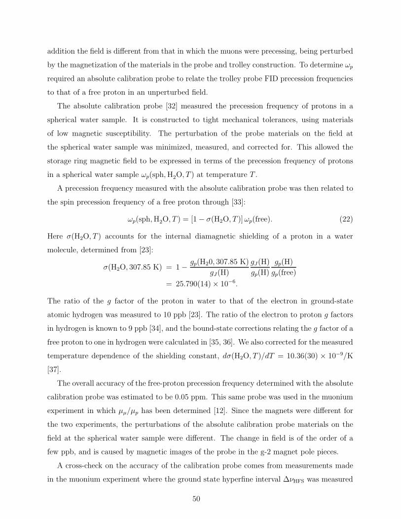
addition the field is different from that in which the muons were precessing, being perturbed
by the magnetization of the materials in the probe and trolley construction. To determine ωp
required an absolute calibration probe to relate the trolley probe FID precession frequencies
to that of a free proton in an unperturbed field.
The absolute calibration probe [32] measured the precession frequency of protons in a
spherical water sample. It is constructed to tight mechanical tolerances, using materials
of low magnetic susceptibility. The perturbation of the probe materials on the field at
the spherical water sample was minimized, measured, and corrected for. This allowed the
storage ring magnetic field to be expressed in terms of the precession frequency of protons
in a spherical water sample ωp(sph,H2O, T ) at temperature T .
A precession frequency measured with the absolute calibration probe was then related to
the spin precession frequency of a free proton through [33]:
ωp(sph,H2O, T ) = [1 − σ(H2O, T )]ωp(free). (22)
Here σ(H2O, T ) accounts for the internal diamagnetic shielding of a proton in a water
molecule, determined from [23]:
σ(H2O, 307.85 K) = 1 − gp(H20, 307.85 K)
gJ(H)
gJ(H)
gp(H)
gp(H)
gp(free)
= 25.790(14) × 10−6.
The ratio of the g factor of the proton in water to that of the electron in ground-state
atomic hydrogen was measured to 10 ppb [23]. The ratio of the electron to proton g factors
in hydrogen is known to 9 ppb [34], and the bound-state corrections relating the g factor of a
free proton to one in hydrogen were calculated in [35, 36]. We also corrected for the measured
temperature dependence of the shielding constant, dσ(H2O, T )/dT = 10.36(30) × 10−9/K
[37].
The overall accuracy of the free-proton precession frequency determined with the absolute
calibration probe was estimated to be 0.05 ppm. This same probe was used in the muonium
experiment in which µµ/µp has been determined [12]. Since the magnets were different for
the two experiments, the perturbations of the absolute calibration probe materials on the
field at the spherical water sample were different. The change in field is of the order of a
few ppb, and is caused by magnetic images of the probe in the g-2 magnet pole pieces.
A cross-check on the accuracy of the calibration probe comes from measurements made
in the muonium experiment where the ground state hyperfine interval ∆νHFS was measured
50
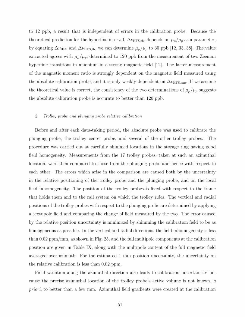
to 12 ppb, a result that is independent of errors in the calibration probe. Because the
theoretical prediction for the hyperfine interval, ∆νHFS,th, depends on µµ/µp as a parameter,
by equating ∆νHFS and ∆νHFS,th, we can determine µµ/µp to 30 ppb [12, 33, 38]. The value
extracted agrees with µµ/µp, determined to 120 ppb from the measurement of two Zeeman
hyperfine transitions in muonium in a strong magnetic field [12]. The latter measurement
of the magnetic moment ratio is strongly dependent on the magnetic field measured using
the absolute calibration probe, and it is only weakly dependent on ∆νHFS,exp. If we assume
the theoretical value is correct, the consistency of the two determinations of µµ/µp suggests
the absolute calibration probe is accurate to better than 120 ppb.
2. Trolley probe and plunging probe relative calibration
Before and after each data-taking period, the absolute probe was used to calibrate the
plunging probe, the trolley center probe, and several of the other trolley probes. The
procedure was carried out at carefully shimmed locations in the storage ring having good
field homogeneity. Measurements from the 17 trolley probes, taken at such an azimuthal
location, were then compared to those from the plunging probe and hence with respect to
each other. The errors which arise in the comparison are caused both by the uncertainty
in the relative positioning of the trolley probe and the plunging probe, and on the local
field inhomogeneity. The position of the trolley probes is fixed with respect to the frame
that holds them and to the rail system on which the trolley rides. The vertical and radial
positions of the trolley probes with respect to the plunging probe are determined by applying
a sextupole field and comparing the change of field measured by the two. The error caused
by the relative position uncertainty is minimized by shimming the calibration field to be as
homogeneous as possible. In the vertical and radial directions, the field inhomogeneity is less
than 0.02 ppm/mm, as shown in Fig. 25, and the full multipole components at the calibration
position are given in Table IX, along with the multipole content of the full magnetic field
averaged over azimuth. For the estimated 1 mm position uncertainty, the uncertainty on
the relative calibration is less than 0.02 ppm.
Field variation along the azimuthal direction also leads to calibration uncertainties be-
cause the precise azimuthal location of the trolley probe’s active volume is not known, a
priori, to better than a few mm. Azimuthal field gradients were created at the calibration
51
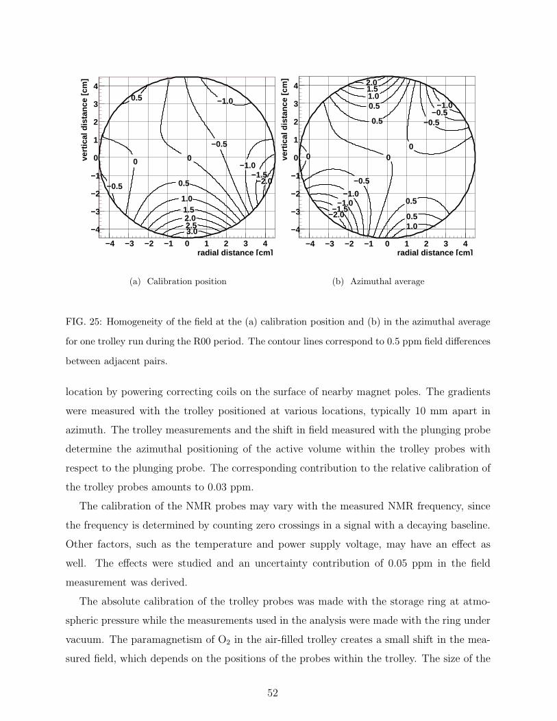
radial distance [cm]−4 −3 −2 −1 0 1 2 3 4
vert
ical
dis
tanc
e [c
m]
−4
−3
−2
−1
0
1
2
3
4
−2.0−1.5
−1.0
−1.0
−0.5
−0.5
00
0.5
3.0
0.5
1.01.52.02.5
(a) Calibration position
radial distance [cm]−4 −3 −2 −1 0 1 2 3 4
vert
ical
dis
tanc
e [c
m]
−4
−3
−2
−1
0
1
2
3
4
−2.0−1.5
−1.0
−1.0
−0.5
−1.0
−0.5
−0.5
000
0.5
0.5
0.5
1.0
1.01.52.0
0.5
(b) Azimuthal average
FIG. 25: Homogeneity of the field at the (a) calibration position and (b) in the azimuthal average
for one trolley run during the R00 period. The contour lines correspond to 0.5 ppm field differences
between adjacent pairs.
location by powering correcting coils on the surface of nearby magnet poles. The gradients
were measured with the trolley positioned at various locations, typically 10 mm apart in
azimuth. The trolley measurements and the shift in field measured with the plunging probe
determine the azimuthal positioning of the active volume within the trolley probes with
respect to the plunging probe. The corresponding contribution to the relative calibration of
the trolley probes amounts to 0.03 ppm.
The calibration of the NMR probes may vary with the measured NMR frequency, since
the frequency is determined by counting zero crossings in a signal with a decaying baseline.
Other factors, such as the temperature and power supply voltage, may have an effect as
well. The effects were studied and an uncertainty contribution of 0.05 ppm in the field
measurement was derived.
The absolute calibration of the trolley probes was made with the storage ring at atmo-
spheric pressure while the measurements used in the analysis were made with the ring under
vacuum. The paramagnetism of O2 in the air-filled trolley creates a small shift in the mea-
sured field, which depends on the positions of the probes within the trolley. The size of the
52
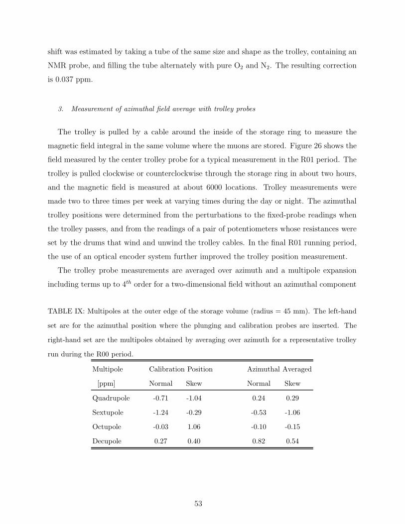
shift was estimated by taking a tube of the same size and shape as the trolley, containing an
NMR probe, and filling the tube alternately with pure O2 and N2. The resulting correction
is 0.037 ppm.
3. Measurement of azimuthal field average with trolley probes
The trolley is pulled by a cable around the inside of the storage ring to measure the
magnetic field integral in the same volume where the muons are stored. Figure 26 shows the
field measured by the center trolley probe for a typical measurement in the R01 period. The
trolley is pulled clockwise or counterclockwise through the storage ring in about two hours,
and the magnetic field is measured at about 6000 locations. Trolley measurements were
made two to three times per week at varying times during the day or night. The azimuthal
trolley positions were determined from the perturbations to the fixed-probe readings when
the trolley passes, and from the readings of a pair of potentiometers whose resistances were
set by the drums that wind and unwind the trolley cables. In the final R01 running period,
the use of an optical encoder system further improved the trolley position measurement.
The trolley probe measurements are averaged over azimuth and a multipole expansion
including terms up to 4th order for a two-dimensional field without an azimuthal component
TABLE IX: Multipoles at the outer edge of the storage volume (radius = 45 mm). The left-hand
set are for the azimuthal position where the plunging and calibration probes are inserted. The
right-hand set are the multipoles obtained by averaging over azimuth for a representative trolley
run during the R00 period.
Multipole Calibration Position Azimuthal Averaged
[ppm] Normal Skew Normal Skew
Quadrupole -0.71 -1.04 0.24 0.29
Sextupole -1.24 -0.29 -0.53 -1.06
Octupole -0.03 1.06 -0.10 -0.15
Decupole 0.27 0.40 0.82 0.54
53
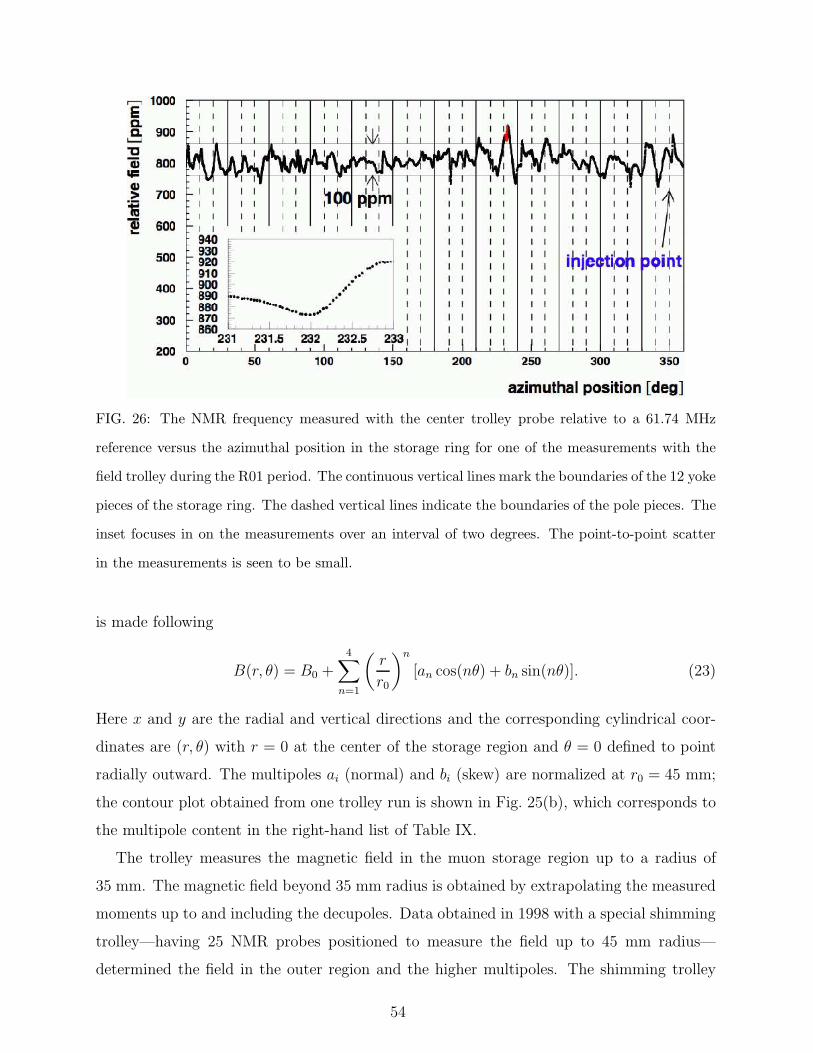
FIG. 26: The NMR frequency measured with the center trolley probe relative to a 61.74 MHz
reference versus the azimuthal position in the storage ring for one of the measurements with the
field trolley during the R01 period. The continuous vertical lines mark the boundaries of the 12 yoke
pieces of the storage ring. The dashed vertical lines indicate the boundaries of the pole pieces. The
inset focuses in on the measurements over an interval of two degrees. The point-to-point scatter
in the measurements is seen to be small.
is made following
B(r, θ) = B0 +4∑
n=1
(r
r0
)n
[an cos(nθ) + bn sin(nθ)]. (23)
Here x and y are the radial and vertical directions and the corresponding cylindrical coor-
dinates are (r, θ) with r = 0 at the center of the storage region and θ = 0 defined to point
radially outward. The multipoles ai (normal) and bi (skew) are normalized at r0 = 45 mm;
the contour plot obtained from one trolley run is shown in Fig. 25(b), which corresponds to
the multipole content in the right-hand list of Table IX.
The trolley measures the magnetic field in the muon storage region up to a radius of
35 mm. The magnetic field beyond 35 mm radius is obtained by extrapolating the measured
moments up to and including the decupoles. Data obtained in 1998 with a special shimming
trolley—having 25 NMR probes positioned to measure the field up to 45 mm radius—
determined the field in the outer region and the higher multipoles. The shimming trolley
54
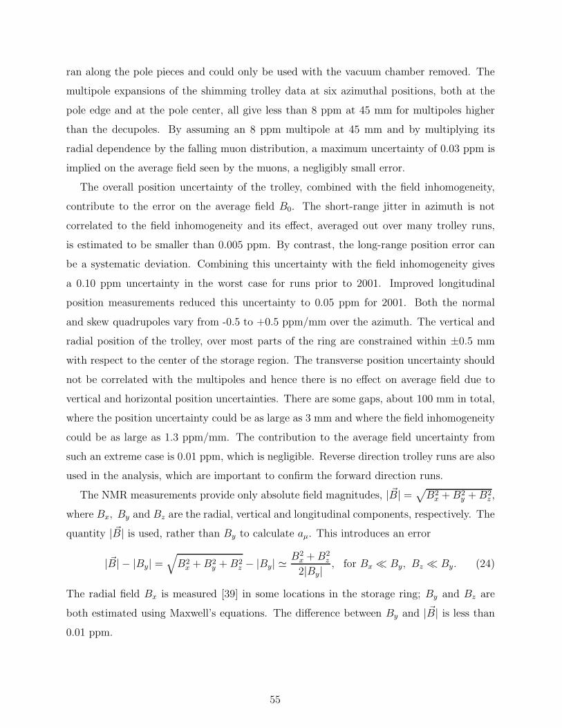
ran along the pole pieces and could only be used with the vacuum chamber removed. The
multipole expansions of the shimming trolley data at six azimuthal positions, both at the
pole edge and at the pole center, all give less than 8 ppm at 45 mm for multipoles higher
than the decupoles. By assuming an 8 ppm multipole at 45 mm and by multiplying its
radial dependence by the falling muon distribution, a maximum uncertainty of 0.03 ppm is
implied on the average field seen by the muons, a negligibly small error.
The overall position uncertainty of the trolley, combined with the field inhomogeneity,
contribute to the error on the average field B0. The short-range jitter in azimuth is not
correlated to the field inhomogeneity and its effect, averaged out over many trolley runs,
is estimated to be smaller than 0.005 ppm. By contrast, the long-range position error can
be a systematic deviation. Combining this uncertainty with the field inhomogeneity gives
a 0.10 ppm uncertainty in the worst case for runs prior to 2001. Improved longitudinal
position measurements reduced this uncertainty to 0.05 ppm for 2001. Both the normal
and skew quadrupoles vary from -0.5 to +0.5 ppm/mm over the azimuth. The vertical and
radial position of the trolley, over most parts of the ring are constrained within ±0.5 mm
with respect to the center of the storage region. The transverse position uncertainty should
not be correlated with the multipoles and hence there is no effect on average field due to
vertical and horizontal position uncertainties. There are some gaps, about 100 mm in total,
where the position uncertainty could be as large as 3 mm and where the field inhomogeneity
could be as large as 1.3 ppm/mm. The contribution to the average field uncertainty from
such an extreme case is 0.01 ppm, which is negligible. Reverse direction trolley runs are also
used in the analysis, which are important to confirm the forward direction runs.
The NMR measurements provide only absolute field magnitudes, | ~B| =√B2
x +B2y +B2
z ,
where Bx, By and Bz are the radial, vertical and longitudinal components, respectively. The
quantity | ~B| is used, rather than By to calculate aµ. This introduces an error
| ~B| − |By| =√B2
x +B2y +B2
z − |By| ≃B2
x +B2z
2|By|, for Bx ≪ By, Bz ≪ By. (24)
The radial field Bx is measured [39] in some locations in the storage ring; By and Bz are
both estimated using Maxwell’s equations. The difference between By and | ~B| is less than
0.01 ppm.
55
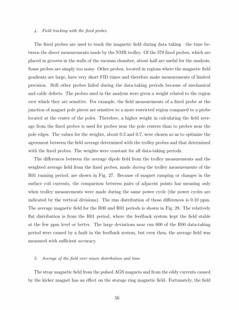
4. Field tracking with the fixed probes
The fixed probes are used to track the magnetic field during data taking—the time be-
tween the direct measurements made by the NMR trolley. Of the 378 fixed probes, which are
placed in grooves in the walls of the vacuum chamber, about half are useful for the analysis.
Some probes are simply too noisy. Other probes, located in regions where the magnetic field
gradients are large, have very short FID times and therefore make measurements of limited
precision. Still other probes failed during the data-taking periods because of mechanical
and cable defects. The probes used in the analysis were given a weight related to the region
over which they are sensitive. For example, the field measurements of a fixed probe at the
junction of magnet pole pieces are sensitive to a more restricted region compared to a probe
located at the center of the poles. Therefore, a higher weight in calculating the field aver-
age from the fixed probes is used for probes near the pole centers than to probes near the
pole edges. The values for the weights, about 0.3 and 0.7, were chosen so as to optimize the
agreement between the field average determined with the trolley probes and that determined
with the fixed probes. The weights were constant for all data-taking periods.
The differences between the average dipole field from the trolley measurements and the
weighted average field from the fixed probes, made during the trolley measurements of the
R01 running period, are shown in Fig. 27. Because of magnet ramping or changes in the
surface coil currents, the comparison between pairs of adjacent points has meaning only
when trolley measurements were made during the same power cycle (the power cycles are
indicated by the vertical divisions). The rms distribution of those differences is 0.10 ppm.
The average magnetic field for the R00 and R01 periods is shown in Fig. 28. The relatively
flat distribution is from the R01 period, where the feedback system kept the field stable
at the few ppm level or better. The large deviations near run 600 of the R00 data-taking
period were caused by a fault in the feedback system, but even then, the average field was
measured with sufficient accuracy.
5. Average of the field over muon distribution and time
The stray magnetic field from the pulsed AGS magnets and from the eddy currents caused
by the kicker magnet has an effect on the storage ring magnetic field. Fortunately, the field
56
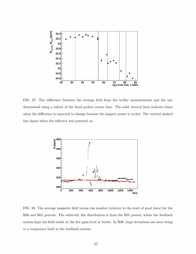
day from Feb. 1 200120 30 40 50 60 70 80 90
[p
pm
]0,
fp-B
0,tr
olle
yB
24.6
24.8
25
25.2
25.4
25.6
25.8
26
26.2
26.4
FIG. 27: The difference between the average field from the trolley measurements and the one
determined using a subset of the fixed probes versus time. The solid vertical lines indicate times
when the difference is expected to change because the magnet power is cycled. The vertical dashed
line shows when the inflector was powered on.
Run0 200 400 600 800 1000 1200 1400
B [
pp
m]
800
810
820
830
840
850
FIG. 28: The average magnetic field versus run number (relative to the start of good data) for the
R00 and R01 periods. The relatively flat distribution is from the R01 period, where the feedback
system kept the field stable at the few ppm level or better. In R00, large deviations are seen owing
to a temporary fault in the feedback system.
57
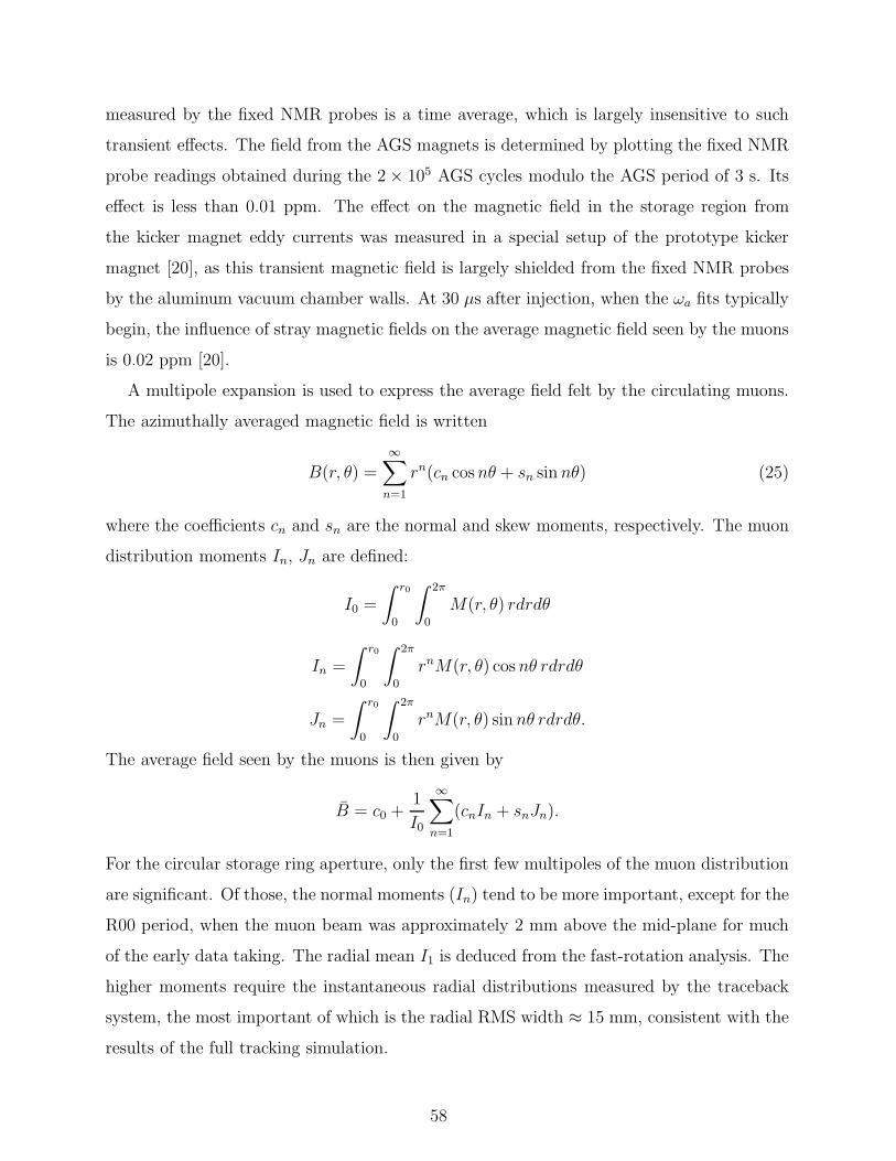
measured by the fixed NMR probes is a time average, which is largely insensitive to such
transient effects. The field from the AGS magnets is determined by plotting the fixed NMR
probe readings obtained during the 2 × 10⁵ AGS cycles modulo the AGS period of 3 s. Its
effect is less than 0.01 ppm. The effect on the magnetic field in the storage region from
the kicker magnet eddy currents was measured in a special setup of the prototype kicker
magnet [20], as this transient magnetic field is largely shielded from the fixed NMR probes
by the aluminum vacuum chamber walls. At 30 µs after injection, when the ωa fits typically
begin, the influence of stray magnetic fields on the average magnetic field seen by the muons
is 0.02 ppm [20].
A multipole expansion is used to express the average field felt by the circulating muons.
The azimuthally averaged magnetic field is written
B(r, θ) =
∞∑
n=1
rn(cn cosnθ + sn sin nθ) (25)
where the coefficients cn and sn are the normal and skew moments, respectively. The muon
distribution moments In, Jn are defined:
I0 =
∫ r0
0
∫ 2π
0
M(r, θ) rdrdθ
In =
∫ r0
0
∫ 2π
0
rnM(r, θ) cos nθ rdrdθ
Jn =
∫ r0
0
∫ 2π
0
rnM(r, θ) sin nθ rdrdθ.
The average field seen by the muons is then given by
B = c0 +1
I0
∞∑
n=1
(cnIn + snJn).
For the circular storage ring aperture, only the first few multipoles of the muon distribution
are significant. Of those, the normal moments (In) tend to be more important, except for the
R00 period, when the muon beam was approximately 2 mm above the mid-plane for much
of the early data taking. The radial mean I1 is deduced from the fast-rotation analysis. The
higher moments require the instantaneous radial distributions measured by the traceback
system, the most important of which is the radial RMS width ≈ 15 mm, consistent with the
results of the full tracking simulation.
58
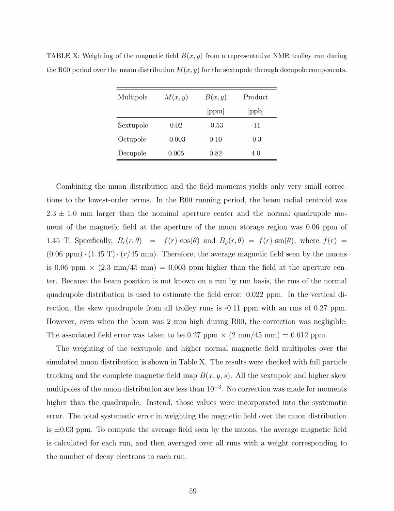
TABLE X: Weighting of the magnetic field B(x, y) from a representative NMR trolley run during
the R00 period over the muon distribution M(x, y) for the sextupole through decupole components.
Multipole M(x, y) B(x, y) Product
[ppm] [ppb]
Sextupole 0.02 -0.53 -11
Octupole -0.003 0.10 -0.3
Decupole 0.005 0.82 4.0
Combining the muon distribution and the field moments yields only very small correc-
tions to the lowest-order terms. In the R00 running period, the beam radial centroid was
2.3 ± 1.0 mm larger than the nominal aperture center and the normal quadrupole mo-
ment of the magnetic field at the aperture of the muon storage region was 0.06 ppm of
1.45 T. Specifically, Br(r, θ) = f(r) cos(θ) and By(r, θ) = f(r) sin(θ), where f(r) =
(0.06 ppm) · (1.45 T) · (r/45 mm). Therefore, the average magnetic field seen by the muons
is 0.06 ppm × (2.3 mm/45 mm) = 0.003 ppm higher than the field at the aperture cen-
ter. Because the beam position is not known on a run by run basis, the rms of the normal
quadrupole distribution is used to estimate the field error: 0.022 ppm. In the vertical di-
rection, the skew quadrupole from all trolley runs is -0.11 ppm with an rms of 0.27 ppm.
However, even when the beam was 2 mm high during R00, the correction was negligible.
The associated field error was taken to be 0.27 ppm × (2 mm/45 mm) = 0.012 ppm.
The weighting of the sextupole and higher normal magnetic field multipoles over the
simulated muon distribution is shown in Table X. The results were checked with full particle
tracking and the complete magnetic field map B(x, y, s). All the sextupole and higher skew
multipoles of the muon distribution are less than 10−3. No correction was made for moments
higher than the quadrupole. Instead, those values were incorporated into the systematic
error. The total systematic error in weighting the magnetic field over the muon distribution
is ±0.03 ppm. To compute the average field seen by the muons, the average magnetic field
is calculated for each run, and then averaged over all runs with a weight corresponding to
the number of decay electrons in each run.
59
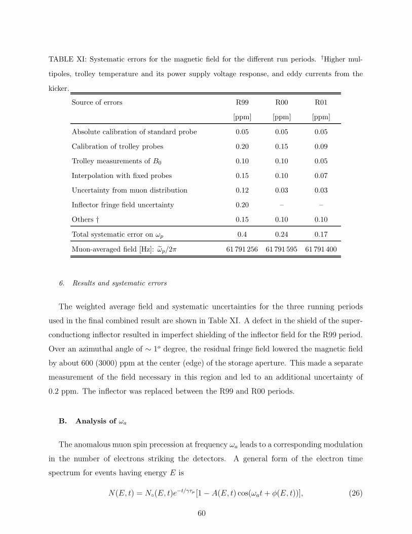
TABLE XI: Systematic errors for the magnetic field for the different run periods. †Higher mul-
tipoles, trolley temperature and its power supply voltage response, and eddy currents from the
kicker.
Source of errors R99 R00 R01
[ppm] [ppm] [ppm]
Absolute calibration of standard probe 0.05 0.05 0.05
Calibration of trolley probes 0.20 0.15 0.09
Trolley measurements of B0 0.10 0.10 0.05
Interpolation with fixed probes 0.15 0.10 0.07
Uncertainty from muon distribution 0.12 0.03 0.03
Inflector fringe field uncertainty 0.20 – –
Others † 0.15 0.10 0.10
Total systematic error on ωp 0.4 0.24 0.17
Muon-averaged field [Hz]: ωp/2π 61 791 256 61 791 595 61 791 400
6. Results and systematic errors
The weighted average field and systematic uncertainties for the three running periods
used in the final combined result are shown in Table XI. A defect in the shield of the super-
conductiong inflector resulted in imperfect shielding of the inflector field for the R99 period.
Over an azimuthal angle of ∼ 1o degree, the residual fringe field lowered the magnetic field
by about 600 (3000) ppm at the center (edge) of the storage aperture. This made a separate
measurement of the field necessary in this region and led to an additional uncertainty of
0.2 ppm. The inflector was replaced between the R99 and R00 periods.
B. Analysis of ωa
The anomalous muon spin precession at frequency ωa leads to a corresponding modulation
in the number of electrons striking the detectors. A general form of the electron time
spectrum for events having energy E is
N(E, t) = N(E, t)e−t/γτµ [1 −A(E, t) cos(ωat+ φ(E, t))], (26)
60
where explicit energy and time dependencies for the normalization, asymmetry and phase
are included. The replacement E → Eth is a convenient simplification of Eq. 26 when the
spectra include all events above energy threshold Eth. An example of a histogram of the
decay electron data from the R01 period was presented in Fig. 2. The anomalous spin
precession frequency ωa, having period τa = 2π/ωa ≈ 4.365 µs, is the prominent feature.
The asymmetry A(Eth, t) is ≈ 0.4, as the threshold energy in this histogram is 1.8 GeV. The
time-dilated muon lifetime is γτµ ≈ 64.4 µs.
The only kinematic cut applied in the ωa analysis is the energy of a given event; it
is therefore important to establish the dependence of the fit parameters on energy. For
example, N(E) (integrated over all decay times, t) is a gradually falling distribution in the
ideal case, having an endpoint at 3.1 GeV (see Fig. 1b). Because of the size of the detectors
and their placement around the storage ring, their acceptance is a strong function of energy.
At 1.8 GeV, it is approximately 65 percent and the acceptance drops with decreasing energy
because low-energy electrons, having small bending radii, can curl between detector stations.
At higher energies, the acceptance rises slowly until, close to 3.1 GeV, the bending radii are
nearly equal to the storage ring radius. These electrons strike the outer radial edge of a
calorimeter, where they are poorly measured because of incomplete shower containment.
Obstacles inside the storage aperture that are in the path of decay electrons (quadrupole
and kicker plates, the vacuum chamber wall) can initiate partial showering, with the result
that a higher-energy electron appears in the detectors as a lower-energy event. The observed
energy spectrum is shown in the inset to Fig. 32. In the ideal case, the asymmetry A is also
a monotonically increasing function of energy, starting at -0.2 for E = 0 and rising to +1 at
3.1 GeV. It crosses 0 at approximately 1.1 GeV. Because of upstream showering and finite
energy resolution, the measured asymmetry differs from expectation.
The phase φ(E) represents the average muon spin angle as a function of energy at t = 0.
It is maximally correlated to ωa in the fitting procedure. In the ideal case, the energy
dependence is trivial. The phase angle is constant for E above the nominal threshold.
The actual shape is explained by two geometrical considerations, both of which depend on
energy. The time assigned to a decay electron corresponds to the arrival at the detector, not
to the decay. High-energy electrons are assigned times later after the decay than low-energy
electrons because their average path length to the detector is longer. In addition, the detector
acceptance is slightly greater when the electron decay angle is inward—toward the center of
61
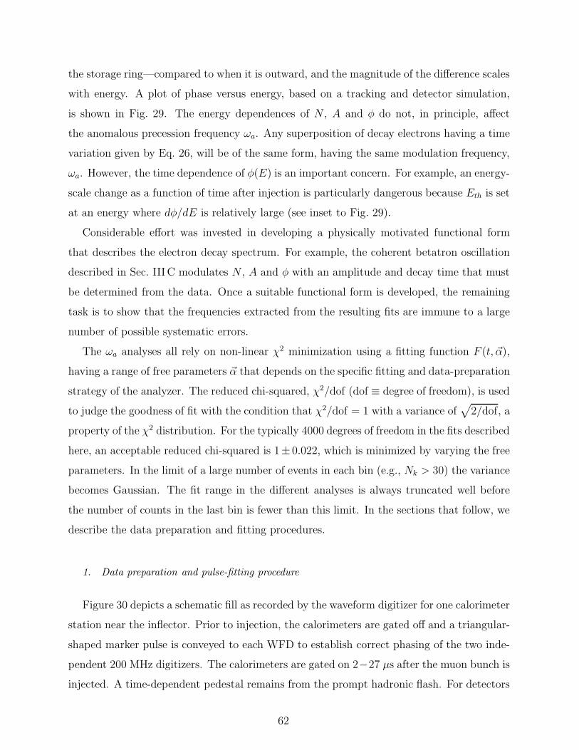
the storage ring—compared to when it is outward, and the magnitude of the difference scales
with energy. A plot of phase versus energy, based on a tracking and detector simulation,
is shown in Fig. 29. The energy dependences of N , A and φ do not, in principle, affect
the anomalous precession frequency ωa. Any superposition of decay electrons having a time
variation given by Eq. 26, will be of the same form, having the same modulation frequency,
ωa. However, the time dependence of φ(E) is an important concern. For example, an energy-
scale change as a function of time after injection is particularly dangerous because Eth is set
at an energy where dφ/dE is relatively large (see inset to Fig. 29).
Considerable effort was invested in developing a physically motivated functional form
that describes the electron decay spectrum. For example, the coherent betatron oscillation
described in Sec. IIIC modulates N , A and φ with an amplitude and decay time that must
be determined from the data. Once a suitable functional form is developed, the remaining
task is to show that the frequencies extracted from the resulting fits are immune to a large
number of possible systematic errors.
The ωa analyses all rely on non-linear χ2 minimization using a fitting function F (t, ~α),
having a range of free parameters ~α that depends on the specific fitting and data-preparation
strategy of the analyzer. The reduced chi-squared, χ2/dof (dof ≡ degree of freedom), is used
to judge the goodness of fit with the condition that χ2/dof = 1 with a variance of√
2/dof, a
property of the χ2 distribution. For the typically 4000 degrees of freedom in the fits described
here, an acceptable reduced chi-squared is 1± 0.022, which is minimized by varying the free
parameters. In the limit of a large number of events in each bin (e.g., Nk > 30) the variance
becomes Gaussian. The fit range in the different analyses is always truncated well before
the number of counts in the last bin is fewer than this limit. In the sections that follow, we
describe the data preparation and fitting procedures.
1. Data preparation and pulse-fitting procedure
Figure 30 depicts a schematic fill as recorded by the waveform digitizer for one calorimeter
station near the inflector. Prior to injection, the calorimeters are gated off and a triangular-
shaped marker pulse is conveyed to each WFD to establish correct phasing of the two inde-
pendent 200 MHz digitizers. The calorimeters are gated on 2−27 µs after the muon bunch is
injected. A time-dependent pedestal remains from the prompt hadronic flash. For detectors
62
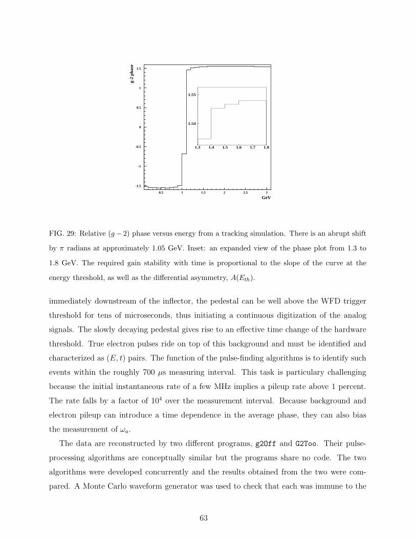
GeV
g-2
phas
e
-1.5
-1
-0.5
0
0.5
1
1.5
0.5 1 1.5 2 2.5 3
1.54
1.55
1.3 1.4 1.5 1.6 1.7 1.8
FIG. 29: Relative (g − 2) phase versus energy from a tracking simulation. There is an abrupt shift
by π radians at approximately 1.05 GeV. Inset: an expanded view of the phase plot from 1.3 to
1.8 GeV. The required gain stability with time is proportional to the slope of the curve at the
energy threshold, as well as the differential asymmetry, A(Eth).
immediately downstream of the inflector, the pedestal can be well above the WFD trigger
threshold for tens of microseconds, thus initiating a continuous digitization of the analog
signals. The slowly decaying pedestal gives rise to an effective time change of the hardware
threshold. True electron pulses ride on top of this background and must be identified and
characterized as (E, t) pairs. The function of the pulse-finding algorithms is to identify such
events within the roughly 700 µs measuring interval. This task is particulary challenging
because the initial instantaneous rate of a few MHz implies a pileup rate above 1 percent.
The rate falls by a factor of 104 over the measurement interval. Because background and
electron pileup can introduce a time dependence in the average phase, they can also bias
the measurement of ωa.
The data are reconstructed by two different programs, g2Off and G2Too. Their pulse-
processing algorithms are conceptually similar but the programs share no code. The two
algorithms were developed concurrently and the results obtained from the two were com-
pared. A Monte Carlo waveform generator was used to check that each was immune to the
63
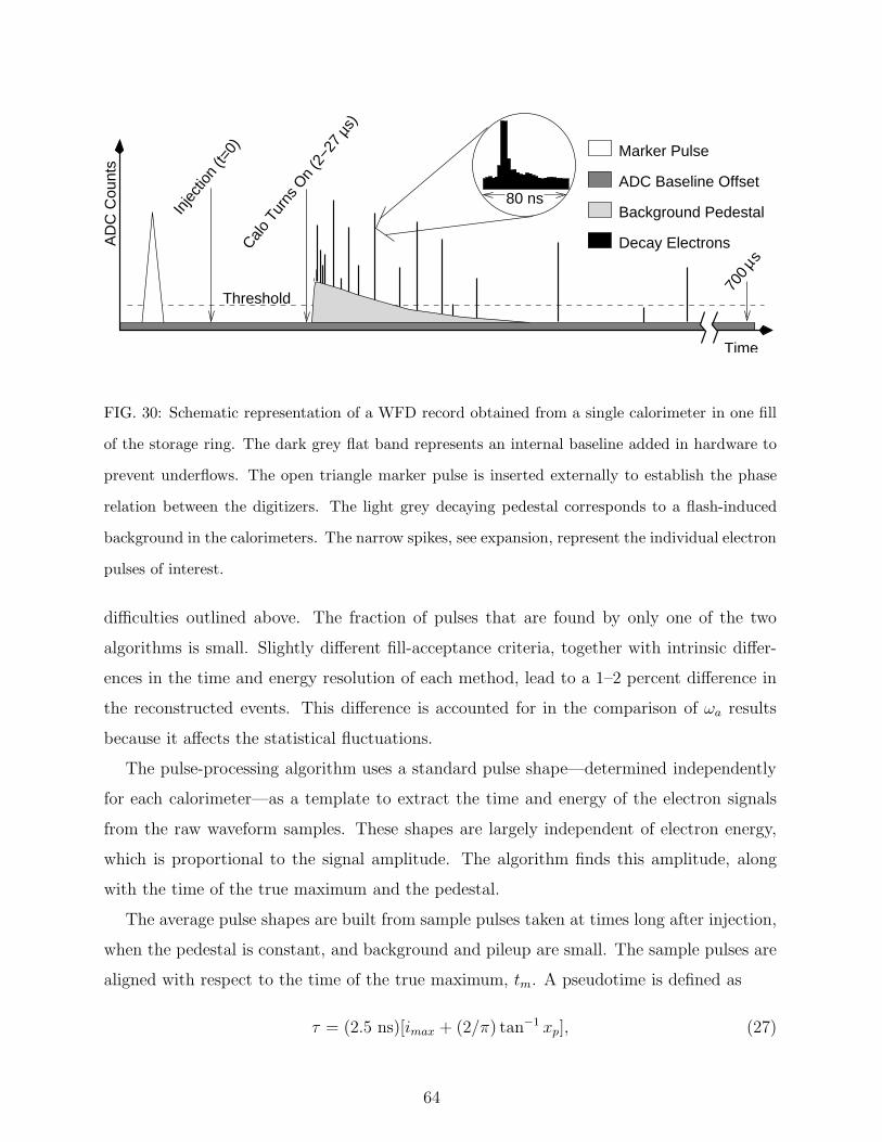
µ
AD
C C
ount
s
80 ns
Marker Pulse
ADC Baseline Offset
Background Pedestal
Decay Electrons
Time
Inje
ctio
n (t=
0)Cal
o Tu
rns
On
(2−2
7 s
)
µ70
0 s
Threshold
FIG. 30: Schematic representation of a WFD record obtained from a single calorimeter in one fill
of the storage ring. The dark grey flat band represents an internal baseline added in hardware to
prevent underflows. The open triangle marker pulse is inserted externally to establish the phase
relation between the digitizers. The light grey decaying pedestal corresponds to a flash-induced
background in the calorimeters. The narrow spikes, see expansion, represent the individual electron
pulses of interest.
difficulties outlined above. The fraction of pulses that are found by only one of the two
algorithms is small. Slightly different fill-acceptance criteria, together with intrinsic differ-
ences in the time and energy resolution of each method, lead to a 1–2 percent difference in
the reconstructed events. This difference is accounted for in the comparison of ωa results
because it affects the statistical fluctuations.
The pulse-processing algorithm uses a standard pulse shape—determined independently
for each calorimeter—as a template to extract the time and energy of the electron signals
from the raw waveform samples. These shapes are largely independent of electron energy,
which is proportional to the signal amplitude. The algorithm finds this amplitude, along
with the time of the true maximum and the pedestal.
The average pulse shapes are built from sample pulses taken at times long after injection,
when the pedestal is constant, and background and pileup are small. The sample pulses are
aligned with respect to the time of the true maximum, tm. A pseudotime is defined as
τ = (2.5 ns)[imax + (2/π) tan−1 xp], (27)
64
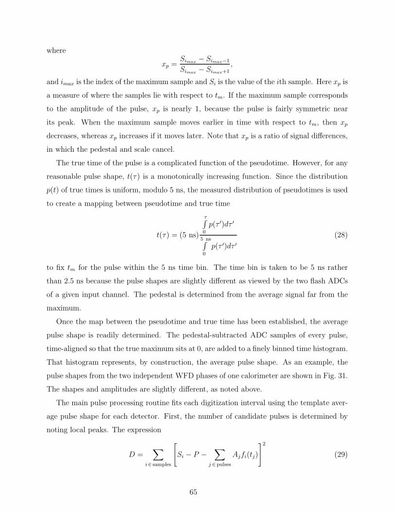
where
xp =Simax
− Simax−1
Simax− Simax+1
,
and imax is the index of the maximum sample and Si is the value of the ith sample. Here xp is
a measure of where the samples lie with respect to tm. If the maximum sample corresponds
to the amplitude of the pulse, xp is nearly 1, because the pulse is fairly symmetric near
its peak. When the maximum sample moves earlier in time with respect to tm, then xp
decreases, whereas xp increases if it moves later. Note that xp is a ratio of signal differences,
in which the pedestal and scale cancel.
The true time of the pulse is a complicated function of the pseudotime. However, for any
reasonable pulse shape, t(τ) is a monotonically increasing function. Since the distribution
p(t) of true times is uniform, modulo 5 ns, the measured distribution of pseudotimes is used
to create a mapping between pseudotime and true time
t(τ) = (5 ns)
τ∫0
p(τ ′)dτ ′
5 ns∫0
p(τ ′)dτ ′(28)
to fix tm for the pulse within the 5 ns time bin. The time bin is taken to be 5 ns rather
than 2.5 ns because the pulse shapes are slightly different as viewed by the two flash ADCs
of a given input channel. The pedestal is determined from the average signal far from the
maximum.
Once the map between the pseudotime and true time has been established, the average
pulse shape is readily determined. The pedestal-subtracted ADC samples of every pulse,
time-aligned so that the true maximum sits at 0, are added to a finely binned time histogram.
That histogram represents, by construction, the average pulse shape. As an example, the
pulse shapes from the two independent WFD phases of one calorimeter are shown in Fig. 31.
The shapes and amplitudes are slightly different, as noted above.
The main pulse processing routine fits each digitization interval using the template aver-
age pulse shape for each detector. First, the number of candidate pulses is determined by
noting local peaks. The expression
D =∑
i∈ samples
[Si − P −
∑
j ∈ pulses
Ajfi(tj)
]2
(29)
65
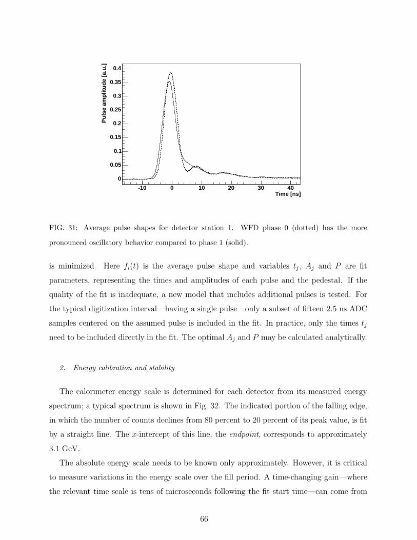
Time [ns]-10 0 10 20 30 40
Pu
lse
amp
litu
de
[a.u
.]
0
0.05
0.1
0.15
0.2
0.25
0.3
0.35
0.4
FIG. 31: Average pulse shapes for detector station 1. WFD phase 0 (dotted) has the more
pronounced oscillatory behavior compared to phase 1 (solid).
is minimized. Here fi(t) is the average pulse shape and variables tj, Aj and P are fit
parameters, representing the times and amplitudes of each pulse and the pedestal. If the
quality of the fit is inadequate, a new model that includes additional pulses is tested. For
the typical digitization interval—having a single pulse—only a subset of fifteen 2.5 ns ADC
samples centered on the assumed pulse is included in the fit. In practice, only the times tj
need to be included directly in the fit. The optimal Aj and P may be calculated analytically.
2. Energy calibration and stability
The calorimeter energy scale is determined for each detector from its measured energy
spectrum; a typical spectrum is shown in Fig. 32. The indicated portion of the falling edge,
in which the number of counts declines from 80 percent to 20 percent of its peak value, is fit
by a straight line. The x-intercept of this line, the endpoint, corresponds to approximately
3.1 GeV.
The absolute energy scale needs to be known only approximately. However, it is critical
to measure variations in the energy scale over the fill period. A time-changing gain—where
the relevant time scale is tens of microseconds following the fit start time—can come from
66
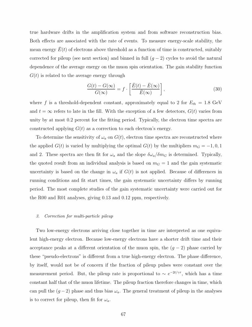
true hardware drifts in the amplification system and from software reconstruction bias.
Both effects are associated with the rate of events. To measure energy-scale stability, the
mean energy E(t) of electrons above threshold as a function of time is constructed, suitably
corrected for pileup (see next section) and binned in full (g − 2) cycles to avoid the natural
dependence of the average energy on the muon spin orientation. The gain stability function
G(t) is related to the average energy through
G(t) −G(∞)
G(∞)= f ·
[E(t) − E(∞)
E(∞)
], (30)
where f is a threshold-dependent constant, approximately equal to 2 for Eth = 1.8 GeV
and t = ∞ refers to late in the fill. With the exception of a few detectors, G(t) varies from
unity by at most 0.2 percent for the fitting period. Typically, the electron time spectra are
constructed applying G(t) as a correction to each electron’s energy.
To determine the sensitivity of ωa on G(t), electron time spectra are reconstructed where
the applied G(t) is varied by multiplying the optimal G(t) by the multipliers mG = −1, 0, 1
and 2. These spectra are then fit for ωa and the slope δωa/δmG is determined. Typically,
the quoted result from an individual analysis is based on mG = 1 and the gain systematic
uncertainty is based on the change in ωa if G(t) is not applied. Because of differences in
running conditions and fit start times, the gain systematic uncertainty differs by running
period. The most complete studies of the gain systematic uncertainty were carried out for
the R00 and R01 analyses, giving 0.13 and 0.12 ppm, respectively.
3. Correction for multi-particle pileup
Two low-energy electrons arriving close together in time are interpreted as one equiva-
lent high-energy electron. Because low-energy electrons have a shorter drift time and their
acceptance peaks at a different orientation of the muon spin, the (g − 2) phase carried by
these “pseudo-electrons” is different from a true high-energy electron. The phase difference,
by itself, would not be of concern if the fraction of pileup pulses were constant over the
measurement period. But, the pileup rate is proportional to ∼ e−2t/γτ , which has a time
constant half that of the muon lifetime. The pileup fraction therefore changes in time, which
can pull the (g− 2) phase and thus bias ωa. The general treatment of pileup in the analyses
is to correct for pileup, then fit for ωa.
67
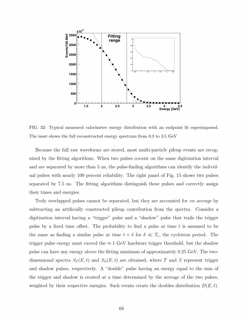
Energy [GeV]1.5 2 2.5 3 3.5 4 4.5
Even
ts/1
00 M
eV
0
500
1000
1500
2000
2500
3000
3500
4x10
Fittingrange
Calorimeter energy [GeV]0.5 1 1.5 2 2.5 3 3.5
N(E
) [a
rb.
un
its
]
0
0.2
0.4
0.6
0.8
1
FIG. 32: Typical measured calorimeter energy distribution with an endpoint fit superimposed.
The inset shows the full reconstructed energy spectrum from 0.3 to 3.5 GeV
Because the full raw waveforms are stored, most multi-particle pileup events are recog-
nized by the fitting algorithms. When two pulses coexist on the same digitization interval
and are separated by more than 5 ns, the pulse-finding algorithms can identify the individ-
ual pulses with nearly 100 percent reliability. The right panel of Fig. 15 shows two pulses
separated by 7.5 ns. The fitting algorithms distinguish these pulses and correctly assign
their times and energies.
Truly overlapped pulses cannot be separated, but they are accounted for on average by
subtracting an artificially constructed pileup contribution from the spectra. Consider a
digitization interval having a “trigger” pulse and a “shadow” pulse that trails the trigger
pulse by a fixed time offset. The probability to find a pulse at time t is assumed to be
the same as finding a similar pulse at time t + δ for δ ≪ Tc, the cyclotron period. The
trigger pulse energy must exceed the ≈ 1 GeV hardware trigger threshold, but the shadow
pulse can have any energy above the fitting minimum of approximately 0.25 GeV. The two-
dimensional spectra ST (E, t) and SS(E, t) are obtained, where T and S represent trigger
and shadow pulses, respectively. A “double” pulse having an energy equal to the sum of
the trigger and shadow is created at a time determined by the average of the two pulses,
weighted by their respective energies. Such events create the doubles distribution D(E, t).
68
Finally, the pileup distribution is
P (E, t) = D(E, t) − ST (E, t) − SS(E, t). (31)
The spectrum of counts can now be corrected for pileup by subtracting this distribu-
tion. In doing so, care must be taken to properly evaluate the errors because some of the
events used to construct the pileup spectrum are part of the uncorrected spectrum already,
depending on the energy cut. To sufficient precision, the uncertainty for a bin in the pileup-
subtracted histogram at time t is described by σ2(t) = (1+k exp(−t/γτµ))F (t), where F (t)
is the functional form describing the pileup-free data and k is determined from the data
itself.
A pileup-free spectrum is created from normalized difference spectra. Figure 33 illus-
trates the uncorrected energy distribution (upper curve), which extends well beyond the
3.1 GeV natural maximum because of pileup events. The artificially constructed pileup
energy distribution is also shown (lower curve). It matches the raw distribution at the high-
est energies, confirming that pileup has been correctly constructed from the raw spectrum.
Below 2.5 GeV, the constructed pileup spectrum is “negative” because two lower-energy
electrons are removed and misinterpreted as a single higher-energy electron; in this figure,
the absolute value is plotted.
The pileup systematic uncertainty falls into three categories: efficiency, phase, and unseen
pileup. The pileup efficiency is established by creating a pileup event spectrum and adding
it to the raw spectrum. A pileup multiplier, mpu, is used to construct modified electron time
distributions with varying pileup fractions. These spectra are fit to determine δωa/δmpu.
Equality of the electron energy spectra early (high rate) and late (low rate) in the fill
indicates that pileup is corrected; an uncertainty of 8 percent on this correction is assigned.
The systematic uncertainty on ωa from pileup subtraction efficiency is 0.036 ppm. The
pileup phase reflects the error due to the uncertainty in the phase of the constructed pileup
spectrum. Simulations determine the limits of the phase difference, and the amplitude
of pileup subtraction, combined with the phase difference, yields an uncertainty in ωa of
0.038 ppm. Finally, a 0.026 ppm uncertainty is assigned to the effect of those very-low-energy
pulses, unnoticed by the pulse-finding algorithm, which are not included in the constructed
pileup spectra. The combined pileup uncertainty on ωa is 0.08 ppm, where the efficiency
and phase uncertainties are correlated and add linearly and the unseen pileup uncertainty
69
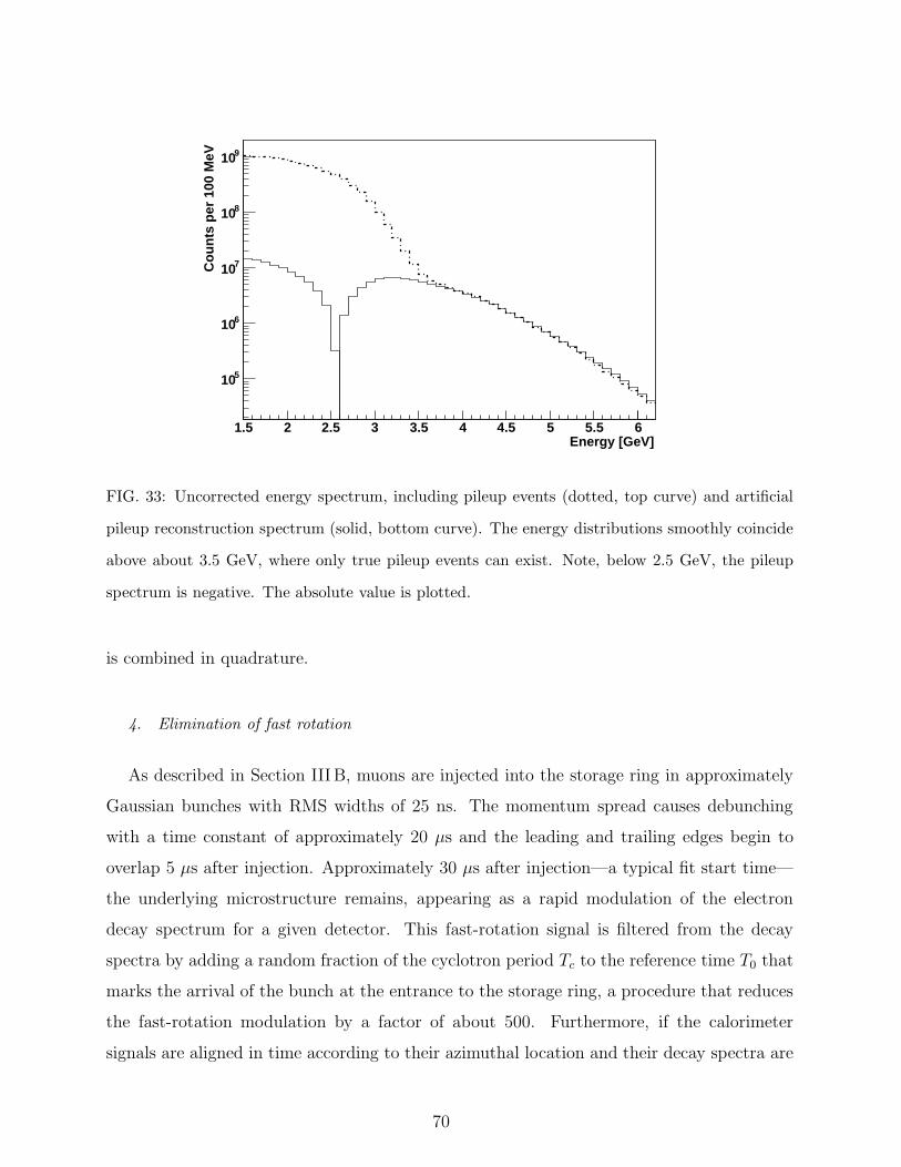
Energy [GeV]1.5 2 2.5 3 3.5 4 4.5 5 5.5 6
Co
un
ts p
er 1
00 M
eV
510
610
710
810
910
FIG. 33: Uncorrected energy spectrum, including pileup events (dotted, top curve) and artificial
pileup reconstruction spectrum (solid, bottom curve). The energy distributions smoothly coincide
above about 3.5 GeV, where only true pileup events can exist. Note, below 2.5 GeV, the pileup
spectrum is negative. The absolute value is plotted.
is combined in quadrature.
4. Elimination of fast rotation
As described in Section IIIB, muons are injected into the storage ring in approximately
Gaussian bunches with RMS widths of 25 ns. The momentum spread causes debunching
with a time constant of approximately 20 µs and the leading and trailing edges begin to
overlap 5 µs after injection. Approximately 30 µs after injection—a typical fit start time—
the underlying microstructure remains, appearing as a rapid modulation of the electron
decay spectrum for a given detector. This fast-rotation signal is filtered from the decay
spectra by adding a random fraction of the cyclotron period Tc to the reference time T0 that
marks the arrival of the bunch at the entrance to the storage ring, a procedure that reduces
the fast-rotation modulation by a factor of about 500. Furthermore, if the calorimeter
signals are aligned in time according to their azimuthal location and their decay spectra are
70
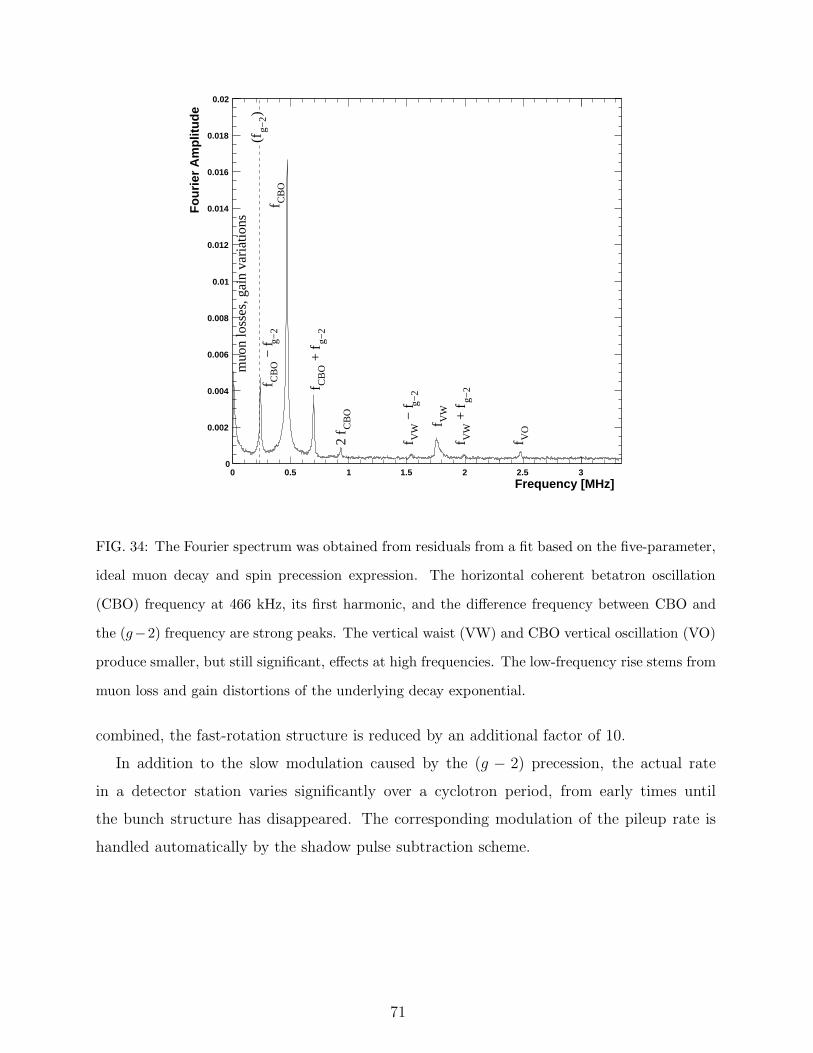
0
0.002
0.004
0.006
0.008
0.01
0.012
0.014
0.016
0.018
0.02
0 0.5 1 1.5 2 2.5 3
Frequency [MHz]
Fo
uri
er A
mp
litu
de
f CB
O
f CB
O +
f
(f
)
g−2
g−2
f CB
O −
f g−2
muo
n lo
sses
, gai
n va
riatio
ns
2 f C
BO
f VW
f VO
f VW
− f g−
2
f VW
+ f
g−2
FIG. 34: The Fourier spectrum was obtained from residuals from a fit based on the five-parameter,
ideal muon decay and spin precession expression. The horizontal coherent betatron oscillation
(CBO) frequency at 466 kHz, its first harmonic, and the difference frequency between CBO and
the (g−2) frequency are strong peaks. The vertical waist (VW) and CBO vertical oscillation (VO)
produce smaller, but still significant, effects at high frequencies. The low-frequency rise stems from
muon loss and gain distortions of the underlying decay exponential.
combined, the fast-rotation structure is reduced by an additional factor of 10.
In addition to the slow modulation caused by the (g − 2) precession, the actual rate
in a detector station varies significantly over a cyclotron period, from early times until
the bunch structure has disappeared. The corresponding modulation of the pileup rate is
handled automatically by the shadow pulse subtraction scheme.
71
5. Multi-parameter fitting
The electron decay spectra prepared as described above, fit with the naive five-parameter
function in Eq. 10, results in a very poor χ2/dof. Fourier analysis of the residuals reveals
identifiable oscillatory features and slow changes to the overall spectral shape. Figure 34
shows the Fourier transform of the residuals of such a fit to the R01 data. While the
fit removes ωa from the residuals, strong peaks at the horizontal CBO frequency, its first
harmonic, and at the sum and difference between the CBO and ωa frequencies are evident.
Additionally, small peaks associated with the vertical CBO (VO) and the vertical waist
(VW) are seen at higher frequencies. The low-frequency rise is ascribed to distortions to
the exponential envelope from muon loss and gain changes. These physical terms motivate
development of a multi-parameter fitting function. A general form, which includes all known
and relevant physical perturbations, and assumes an energy threshold Eth, can be written
N(t) =N0
γτµe−t/γτµ · Λ(t) · V (t) · B(t) · C(t) · [1 − A(t) cos(ωa t+ φ(t)] (32)
with
Λ(t) = 1 − Aloss
∫ t
0
L(t′)e−t′/γτµdt′ (33)
V (t) = 1 − e−t/τV WAV W cos(ωV W t+ φV W ) (34)
B(t) = 1 − Abre−t/τbr (35)
C(t) = 1 − e−t/τcboA1 cos(ωcbo t+ φ1) (36)
A(t) = A(1 − e−t/τcboA2 cos(ωcbo t+ φ2)
)(37)
φ(t) = φ0 + e−t/τcboA3 cos(ωcbo t+ φ3). (38)
While the additional terms are necessary to obtain an acceptable χ2, they are not strongly
correlated to ωa.
Equation 33 describes Λ(t), which is derived from L(t), which in turn is derived from the
muon loss monitor data, as illustrated in Fig. 35. Muon loss introduces a slowly changing
modification to the normal exponential decay. To determine the absolute rate of muon losses,
the acceptance of the detection system must be established by the Monte Carlo simulation.
With an estimated acceptance of a few percent, results from the fits indicate an approximate
fractional loss rate of 10−3 per lifetime.
72
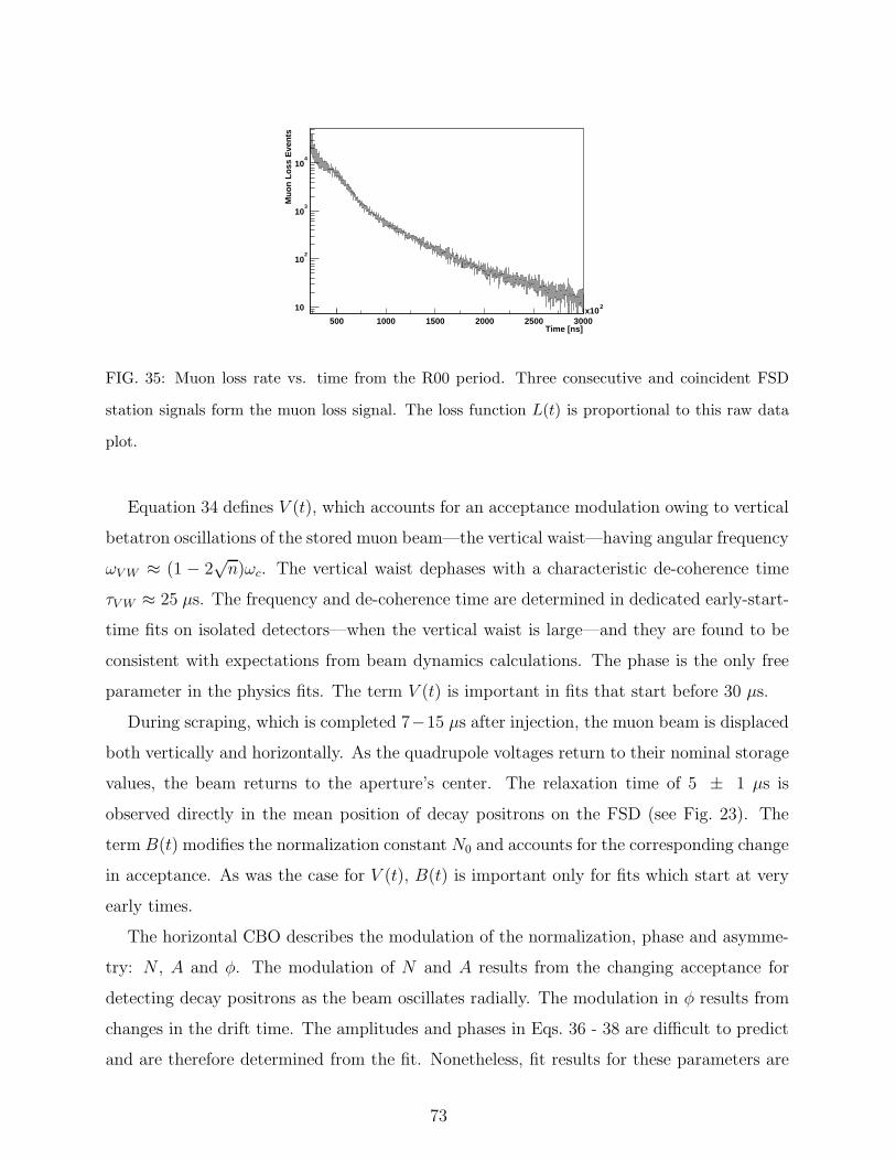
Time [ns]500 1000 1500 2000 2500 3000
2x10
Mu
on
Lo
ss E
ven
ts
10
102
103
104
FIG. 35: Muon loss rate vs. time from the R00 period. Three consecutive and coincident FSD
station signals form the muon loss signal. The loss function L(t) is proportional to this raw data
plot.
Equation 34 defines V (t), which accounts for an acceptance modulation owing to vertical
betatron oscillations of the stored muon beam—the vertical waist—having angular frequency
ωV W ≈ (1 − 2√n)ωc. The vertical waist dephases with a characteristic de-coherence time
τV W ≈ 25 µs. The frequency and de-coherence time are determined in dedicated early-start-
time fits on isolated detectors—when the vertical waist is large—and they are found to be
consistent with expectations from beam dynamics calculations. The phase is the only free
parameter in the physics fits. The term V (t) is important in fits that start before 30 µs.
During scraping, which is completed 7−15 µs after injection, the muon beam is displaced
both vertically and horizontally. As the quadrupole voltages return to their nominal storage
values, the beam returns to the aperture’s center. The relaxation time of 5 ± 1 µs is
observed directly in the mean position of decay positrons on the FSD (see Fig. 23). The
term B(t) modifies the normalization constant N0 and accounts for the corresponding change
in acceptance. As was the case for V (t), B(t) is important only for fits which start at very
early times.
The horizontal CBO describes the modulation of the normalization, phase and asymme-
try: N , A and φ. The modulation of N and A results from the changing acceptance for
detecting decay positrons as the beam oscillates radially. The modulation in φ results from
changes in the drift time. The amplitudes and phases in Eqs. 36 - 38 are difficult to predict
and are therefore determined from the fit. Nonetheless, fit results for these parameters are
73
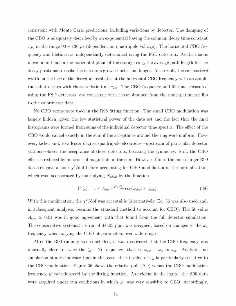
consistent with Monte Carlo predictions, including variations by detector. The damping of
the CBO is adequately described by an exponential having the common decay time constant
τcbo in the range 90 − 130 µs (dependent on quadrupole voltage). The horizontal CBO fre-
quency and lifetime are independently determined using the FSD detectors. As the muons
move in and out in the horizontal plane of the storage ring, the average path length for the
decay positrons to strike the detectors grows shorter and longer. As a result, the rms vertical
width on the face of the detectors oscillates at the horizontal CBO frequency with an ampli-
tude that decays with characteristic time τcbo. The CBO frequency and lifetime, measured
using the FSD detectors, are consistent with those obtained from the multi-parameter fits
to the calorimeter data.
No CBO terms were used in the R98 fitting function. The small CBO modulation was
largely hidden, given the low statistical power of the data set and the fact that the final
histograms were formed from sums of the individual detector time spectra. The effect of the
CBO would cancel exactly in the sum if the acceptance around the ring were uniform. How-
ever, kicker and, to a lesser degree, quadrupole electrodes—upstream of particular detector
stations—lower the acceptance of those detectors, breaking the symmetry. Still, the CBO
effect is reduced by an order of magnitude in the sum. However, fits to the much larger R99
data set gave a poor χ2/dof before accounting for CBO modulation of the normalization,
which was incorporated by multiplying Nideal by the function
C ′(t) = 1 + Acboe−t2/τ2
cbo cos(ωcbot+ φcbo). (39)
With this modification, the χ2/dof was acceptable (alternatively, Eq. 36 was also used and,
in subsequent analyses, became the standard method to account for CBO). The fit value
Acbo ≃ 0.01 was in good agreement with that found from the full detector simulation.
The conservative systematic error of ±0.05 ppm was assigned, based on changes to the ωa
frequency when varying the CBO fit parameters over wide ranges.
After the R00 running was concluded, it was discovered that the CBO frequency was
unusually close to twice the (g − 2) frequency; that is, ωcbo − ωa ≈ ωa. Analytic and
simulation studies indicate that in this case, the fit value of ωa is particularly sensitive to
the CBO modulation. Figure 36 shows the relative pull (∆ω) versus the CBO modulation
frequency if not addressed by the fitting function. As evident in the figure, the R00 data
were acquired under run conditions in which ωa was very sensitive to CBO. Accordingly,
74
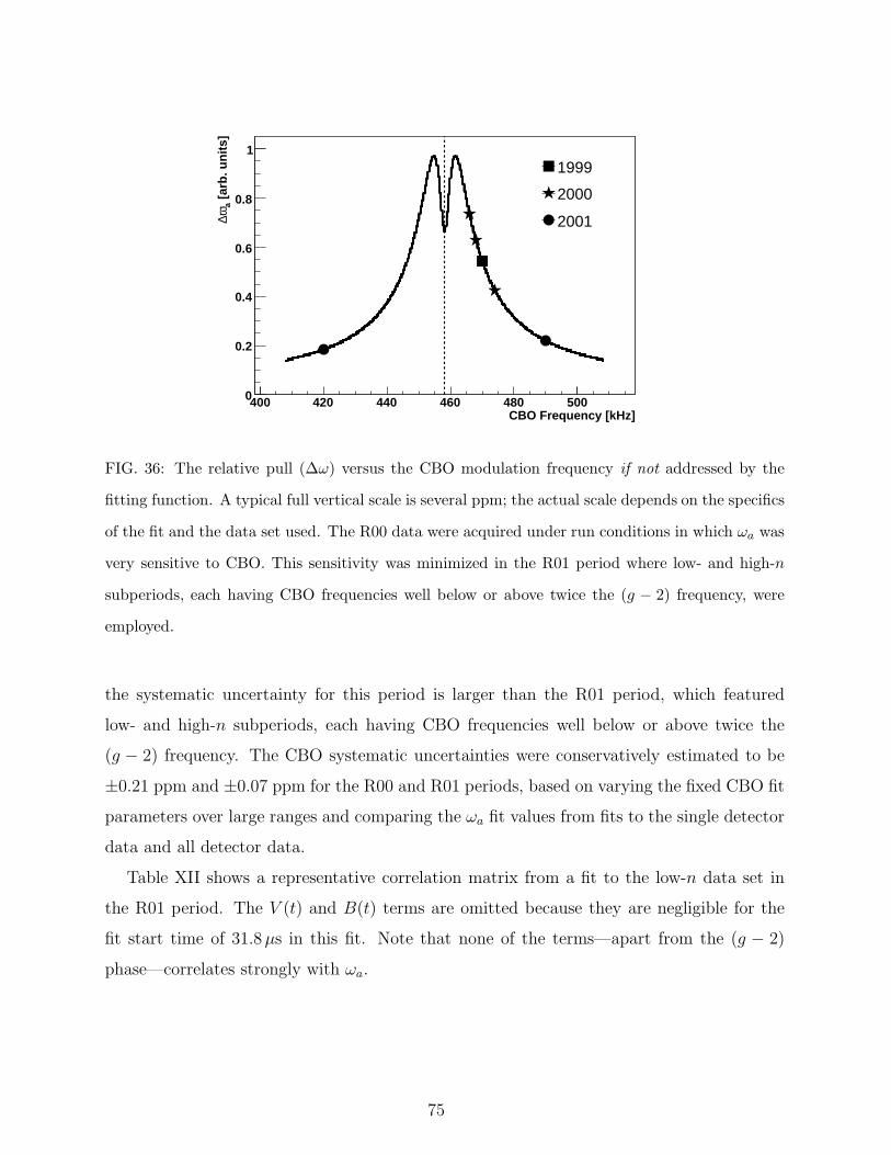
CBO Frequency [kHz]400 420 440 460 480 500
[ar
b. u
nit
s]a
ω∆
0
0.2
0.4
0.6
0.8
1
1999
2000
2001
FIG. 36: The relative pull (∆ω) versus the CBO modulation frequency if not addressed by the
fitting function. A typical full vertical scale is several ppm; the actual scale depends on the specifics
of the fit and the data set used. The R00 data were acquired under run conditions in which ωa was
very sensitive to CBO. This sensitivity was minimized in the R01 period where low- and high-n
subperiods, each having CBO frequencies well below or above twice the (g − 2) frequency, were
employed.
the systematic uncertainty for this period is larger than the R01 period, which featured
low- and high-n subperiods, each having CBO frequencies well below or above twice the
(g − 2) frequency. The CBO systematic uncertainties were conservatively estimated to be
±0.21 ppm and ±0.07 ppm for the R00 and R01 periods, based on varying the fixed CBO fit
parameters over large ranges and comparing the ωa fit values from fits to the single detector
data and all detector data.
Table XII shows a representative correlation matrix from a fit to the low-n data set in
the R01 period. The V (t) and B(t) terms are omitted because they are negligible for the
fit start time of 31.8µs in this fit. Note that none of the terms—apart from the (g − 2)
phase—correlates strongly with ωa.
75
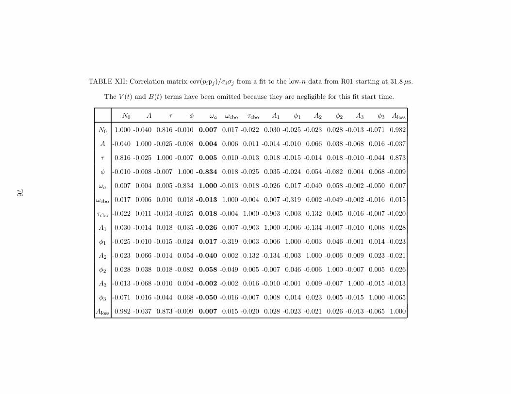
TABLE XII: Correlation matrix cov(pipj)/σiσj from a fit to the low-n data from R01 starting at 31.8 µs.
The V (t) and B(t) terms have been omitted because they are negligible for this fit start time.
N0 A τ φ ωa ωcbo τcbo A1 φ1 A2 φ2 A3 φ3 Aloss
N0 1.000 -0.040 0.816 -0.010 0.007 0.017 -0.022 0.030 -0.025 -0.023 0.028 -0.013 -0.071 0.982
A -0.040 1.000 -0.025 -0.008 0.004 0.006 0.011 -0.014 -0.010 0.066 0.038 -0.068 0.016 -0.037
τ 0.816 -0.025 1.000 -0.007 0.005 0.010 -0.013 0.018 -0.015 -0.014 0.018 -0.010 -0.044 0.873
φ -0.010 -0.008 -0.007 1.000 -0.834 0.018 -0.025 0.035 -0.024 0.054 -0.082 0.004 0.068 -0.009
ωa 0.007 0.004 0.005 -0.834 1.000 -0.013 0.018 -0.026 0.017 -0.040 0.058 -0.002 -0.050 0.007
ωcbo 0.017 0.006 0.010 0.018 -0.013 1.000 -0.004 0.007 -0.319 0.002 -0.049 -0.002 -0.016 0.015
τcbo -0.022 0.011 -0.013 -0.025 0.018 -0.004 1.000 -0.903 0.003 0.132 0.005 0.016 -0.007 -0.020
A1 0.030 -0.014 0.018 0.035 -0.026 0.007 -0.903 1.000 -0.006 -0.134 -0.007 -0.010 0.008 0.028
φ1 -0.025 -0.010 -0.015 -0.024 0.017 -0.319 0.003 -0.006 1.000 -0.003 0.046 -0.001 0.014 -0.023
A2 -0.023 0.066 -0.014 0.054 -0.040 0.002 0.132 -0.134 -0.003 1.000 -0.006 0.009 0.023 -0.021
φ2 0.028 0.038 0.018 -0.082 0.058 -0.049 0.005 -0.007 0.046 -0.006 1.000 -0.007 0.005 0.026
A3 -0.013 -0.068 -0.010 0.004 -0.002 -0.002 0.016 -0.010 -0.001 0.009 -0.007 1.000 -0.015 -0.013
φ3 -0.071 0.016 -0.044 0.068 -0.050 -0.016 -0.007 0.008 0.014 0.023 0.005 -0.015 1.000 -0.065
Aloss 0.982 -0.037 0.873 -0.009 0.007 0.015 -0.020 0.028 -0.023 -0.021 0.026 -0.013 -0.065 1.000
76
6. The ratio-fitting method
An alternative analysis of ωa first randomly sorts the electron time spectra into four equal
subsets, labelled n1(t) through n4(t). Each is similar to the standard N(t) distribution. The
four subsets are then recombined in the ratio
r(t) =n1
(t+ 1
2T
)+ n2
(t− 1
2T
)− n3(t) − n4(t)
n1
(t+ 1
2T
)+ n2
(t− 1
2T
)+ n3(t) + n4(t)
(40)
to produce a spectrum as shown in Fig. 37. Here, T = 2π/ωa is a (very good) estimate of
the spin precession period. In preparing the ratio histograms, gain corrections are applied
to the data and pileup and fast rotation are removed. The ratio histograms can then be fit
well by a three-parameter function, which accounts for the amplitude, frequency and phase
of the spin precession:
r3(t) = A cos(ωa t+ φ) +1
16
(T
γτµ
)2
. (41)
The final term arises from the exponential decay when shifting the subsets forward or back-
ward in time by T/2. Equation 41 describes well the ratio histograms formed when data
from all detectors are combined. In the R01 analysis, it was used successfully to fit the
detector-combined data from both n-value data sets.
However, Eq. 41 is inadequate in fitting individual detector data subsets, or those of a
given field index, as was done in an independent analysis of the R01 data. The ratio function
must be expanded to incorporate the CBO modulation of the normalization, asymmetry and
phase, as described for the multi-parameter fitting. Therefore, Eq. 41 is replaced by the more
general nine-parameter function
r9(t) =2f0(t) − f+(t) − f−(t)
2f0(t) + f+(t) + f−(t)(42)
where
f0(t) = C(t) · (1 + A(t) cos(ωat+ φ(t)) (43)
and
f±(t) = C(t′)e∓T/(2γτµ) · [1 + A(t′) cos(ωat+ φ(t′))] (44)
with C(t), A(t) and φ(t) defined in Eqs. 36, 37, and 38, and with t′ = t±T/2. This expression
is sufficient to obtain good fits to individual data subsets.
77
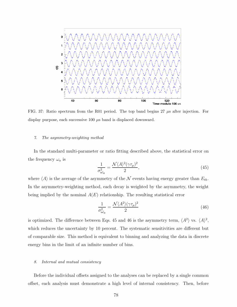
FIG. 37: Ratio spectrum from the R01 period. The top band begins 27 µs after injection. For
display purpose, each successive 100 µs band is displaced downward.
7. The asymmetry-weighting method
In the standard multi-parameter or ratio fitting described above, the statistical error on
the frequency ωa is1
σ2ωa
=N〈A〉2(γτµ)2
2, (45)
where 〈A〉 is the average of the asymmetry of the N events having energy greater than Eth.
In the asymmetry-weighting method, each decay is weighted by the asymmetry, the weight
being implied by the nominal A(E) relationship. The resulting statistical error
1
σ2ωa
=N〈A2〉(γτµ)2
2(46)
is optimized. The difference between Eqs. 45 and 46 is the asymmetry term, 〈A2〉 vs. 〈A〉2,which reduces the uncertainty by 10 percent. The systematic sensitivities are different but
of comparable size. This method is equivalent to binning and analyzing the data in discrete
energy bins in the limit of an infinite number of bins.
8. Internal and mutual consistency
Before the individual offsets assigned to the analyses can be replaced by a single common
offset, each analysis must demonstrate a high level of internal consistency. Then, before
78
the common offset is removed, the results of the different analyses are examined for mutual
consistency.
Internal consistency demands:
• a reduced χ2 equal to unity within the expected statistical spread;
• no pronounced structures in the fit residuals, both in the time and frequency domains;
• that the fit results must be independent of any specific subset of data, within expected
statistical and systematic errors.
The optimal set of parameters is obtained by minimizing χ2, defined as
χ2 =∑
bins
[Ni − F (ti, ~α)]2
σ2i
. (47)
The error σi must account for pileup subtraction. In some analyses it was calculated
during the pileup correction procedure, as a combination of the contents of the bin and the
amount subtracted from that bin. In others, it was approximated as (1 + k e−t/γτ )F (ti, ~α).
The latter method was inspired by the observation that without pileup subtraction, σ2i =
F (ti, ~α), that is the best estimate of the error squared at any point is given by the fit value
itself. The factor (1 + k e−t/γτ ) reflects a small correction because of the pileup subtraction.
The quality of the fits is tested by splitting the data into subsets, especially those that
enhance or reduce particular systematic uncertainties. In estimating the impact of statistical
fluctuations in the comparison of subset fits, the data overlap and change in analyzing power
(notably the asymmetry) has to be taken into account.
Data subset comparisons include:
• Start time: As the fit start times increase, the effects of short time-constant (< γτ)
perturbations—V (t), B(t), fast rotation, pileup, gain changes—disappear. Therefore
the stability of results versus start time is one of the most sensitive measures of a good
fitting function.
• Run conditions: Fits are carried out on individual runs or sets of runs having special
experimental conditions. Examples include variations in n values, quadrupole scraping
voltage or timing, and radial magnetic field. Data from each of the 12 bunches in an
AGS cycle were considered separately and compared.
79
• Electron energy: Data are sorted into discrete energy bins (typically 200 MeV wide)
or into sets having different low-energy thresholds. Fits to these data sets are naturally
quite sensitive to the details of energy scale and pileup corrections.
• Detector: Fits are carried out on data from individual detectors, on detector groups,
and on the sum of all detectors. This division is particularly sensitive to a correct
treatment of CBO and of the early-time background, which are highly dependent on
position around the ring.
Figure 38 is a representative set of important fit subset tests for one of the R00 multi-
parameter analyses. Individual fits all had acceptable reduced χ2. The top left panel shows
the stability of the precession frequency versus start time of the fit. The sideways “parabolic”
band defines the expected range of successive results, given the initial fit value and the steady
diminution of the data set. The outer envelope represents the statistical uncertainty on any
individual fit. The top right panel shows the ωa results for data binned in 200 MeV energy
bands, for a fixed start time. This distribution is flat, as expected. The bottom left panel
shows the result as a function of detector station around the ring [40]. Data were divided
into subsets indexed by both detector number and energy band. The consistency of the ωa
values can be verified by calculating the mean of the ensemble and plotting the deviation of
each individual fit, normalized by the respective statistical error. The result, shown in the
bottom right panel, is a Gaussian of width 1, as expected.
The expected spread in fitting results for data sets that partially overlap depends on the
size of the data samples, as well as on the difference in analyzing power—the asymmetry
and the phase of the (g − 2) modulation—giving
σdiff =
√
σ22 − σ2
1
(2A1
A2cos (φ1 − φ2) − 1
). (48)
Here, the larger data set is indicated by subscript 1 and the smaller, fully-contained subset,
by subscript 2. Data sets having different energy thresholds will have a different analyzing
power. In the case that the analyzing powers are the same (A1 ≃ A2 and φ1 ≃ φ2), Eq. 48
reduces to
σdiff ≃√σ2
2 − σ21 , (49)
a result that is applicable to nearly all of the consistency tests, and is the basis of the
envelope shown in Fig. 38.
80
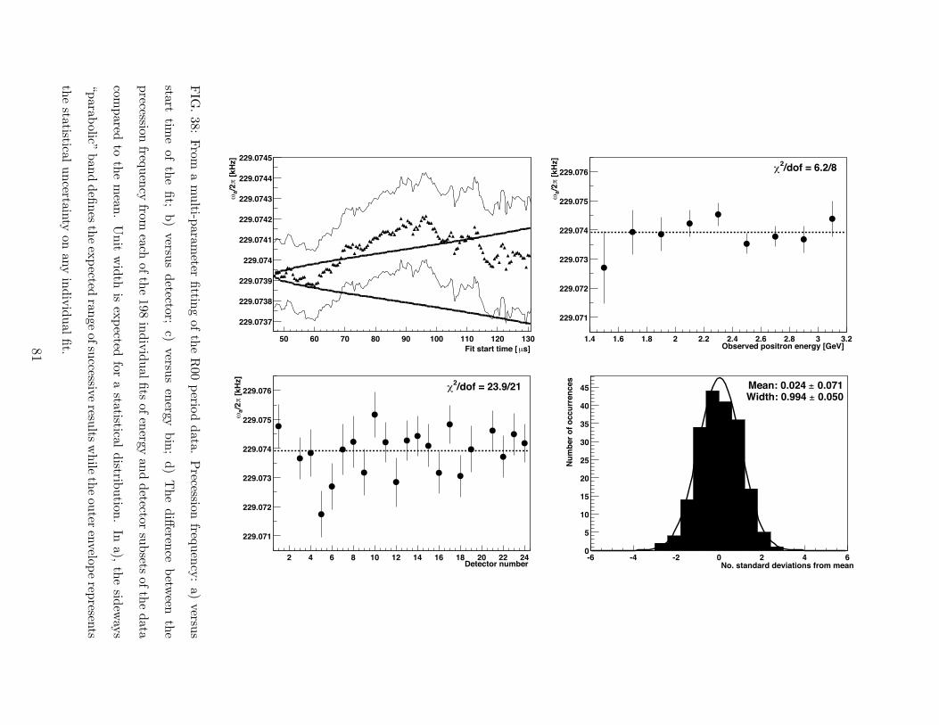
Observed positron energy [GeV]1.4 1.6 1.8 2 2.2 2.4 2.6 2.8 3 3.2
[kH
z]
!/2
a"
229.071
229.072
229.073
229.074
229.075
229.076/dof = 6.2/8
2#
s]!Fit start time [
50 60 70 80 90 100 110 120 130
[kH
z]
!/2
a"
229.0737
229.0738
229.0739
229.074
229.0741
229.0742
229.0743
229.0744
229.0745
Detector number2 4 6 8 10 12 14 16 18 20 22 24
[kH
z]
!/2
a"
229.071
229.072
229.073
229.074
229.075
229.076 /dof = 23.9/212#
(i)$>/a" - <a(i)"
-6 -4 -2 0 2 4 6
Nu
mb
er
of
occu
rren
ces
0
5
10
15
20
25
30
35
40
45 0.071"Mean: 0.024 0.050"Width: 0.994
No. standard deviations from mean
FIG
.38:
From
am
ulti-p
arameter
fittin
gof
the
R00
perio
ddata.
Precession
frequen
cy:
a)versu
s
starttim
eof
the
fit;
b)
versus
detector;
c)versu
sen
ergybin
;d)
The
diff
erence
betw
eenth
e
precession
frequen
cyfrom
eachof
the
198in
div
idual
fits
ofen
ergyan
ddetector
subsets
ofth
edata
compared
toth
em
ean.
Unit
wid
this
expected
fora
statisticaldistrib
ution
.In
a),th
esid
eway
s
“parab
olic”ban
ddefi
nes
the
expected
range
ofsu
ccessiveresu
ltsw
hile
the
outer
envelop
erep
resents
the
statisticaluncertain
tyon
any
indiv
idual
fit.81
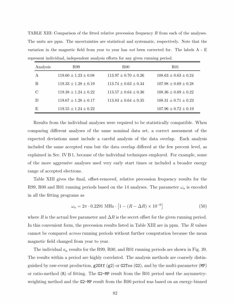
TABLE XIII: Comparison of the fitted relative precession frequency R from each of the analyses.
The units are ppm. The uncertainties are statistical and systematic, respectively. Note that the
variation in the magnetic field from year to year has not been corrected for. The labels A - E
represent individual, independent analysis efforts for any given running period.
Analysis R99 R00 R01
A 119.60 ± 1.23 ± 0.08 113.97 ± 0.70 ± 0.26 108.63 ± 0.63 ± 0.24
B 119.33 ± 1.28 ± 0.19 113.74 ± 0.63 ± 0.34 107.98 ± 0.69 ± 0.28
C 119.38 ± 1.24 ± 0.22 113.57 ± 0.64 ± 0.36 108.36 ± 0.69 ± 0.22
D 119.67 ± 1.28 ± 0.17 113.83 ± 0.64 ± 0.35 108.31 ± 0.71 ± 0.23
E 119.55 ± 1.24 ± 0.22 107.96 ± 0.72 ± 0.19
Results from the individual analyses were required to be statistically compatible. When
comparing different analyses of the same nominal data set, a correct assessment of the
expected deviations must include a careful analysis of the data overlap. Each analysis
included the same accepted runs but the data overlap differed at the few percent level, as
explained in Sec. IVB1, because of the individual techniques employed. For example, some
of the more aggressive analyses used very early start times or included a broader energy
range of accepted electrons.
Table XIII gives the final, offset-removed, relative precession frequency results for the
R99, R00 and R01 running periods based on the 14 analyses. The parameter ωa is encoded
in all the fitting programs as
ωa = 2π · 0.2291 MHz ·[1 − (R− ∆R) × 10−6
](50)
where R is the actual free parameter and ∆R is the secret offset for the given running period.
In this convenient form, the precession results listed in Table XIII are in ppm. The R values
cannot be compared across running periods without further computation because the mean
magnetic field changed from year to year.
The individual aµ results for the R99, R00, and R01 running periods are shown in Fig. 39.
The results within a period are highly correlated. The analysis methods are coarsely distin-
guished by raw-event production, g2Off (g2) or G2Too (G2), and by the multi-parameter (MP)
or ratio-method (R) of fitting. The G2-MP result from the R01 period used the asymmetry-
weighting method and the G2-MP result from the R00 period was based on an energy-binned
82
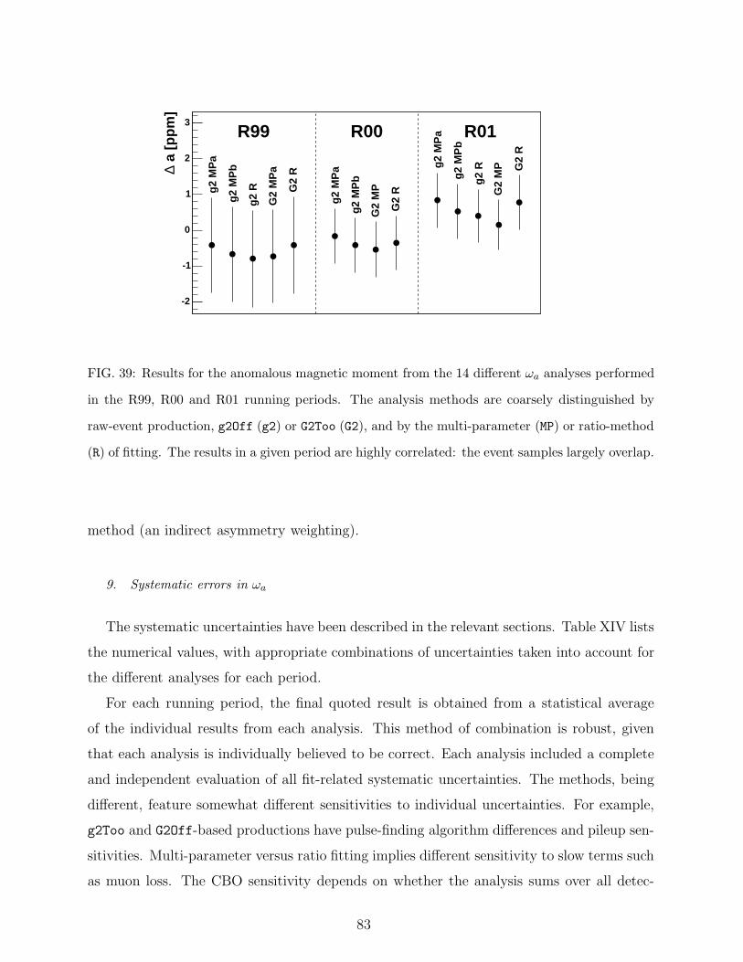
a [
pp
m]
∆
-2
-1
0
1
2
3
g2
MP
a
g2
MP
b
g2
R
G2
MP
a
G2
R
g2
MP
a
g2
MP
b
G2
MP
G2
R
g2
MP
a
g2
MP
b
g2
R
G2
MP G
2 R
R99 R00 R01
FIG. 39: Results for the anomalous magnetic moment from the 14 different ωa analyses performed
in the R99, R00 and R01 running periods. The analysis methods are coarsely distinguished by
raw-event production, g2Off (g2) or G2Too (G2), and by the multi-parameter (MP) or ratio-method
(R) of fitting. The results in a given period are highly correlated: the event samples largely overlap.
method (an indirect asymmetry weighting).
9. Systematic errors in ωa
The systematic uncertainties have been described in the relevant sections. Table XIV lists
the numerical values, with appropriate combinations of uncertainties taken into account for
the different analyses for each period.
For each running period, the final quoted result is obtained from a statistical average
of the individual results from each analysis. This method of combination is robust, given
that each analysis is individually believed to be correct. Each analysis included a complete
and independent evaluation of all fit-related systematic uncertainties. The methods, being
different, feature somewhat different sensitivities to individual uncertainties. For example,
g2Too and G2Off-based productions have pulse-finding algorithm differences and pileup sen-
sitivities. Multi-parameter versus ratio fitting implies different sensitivity to slow terms such
as muon loss. The CBO sensitivity depends on whether the analysis sums over all detec-
83
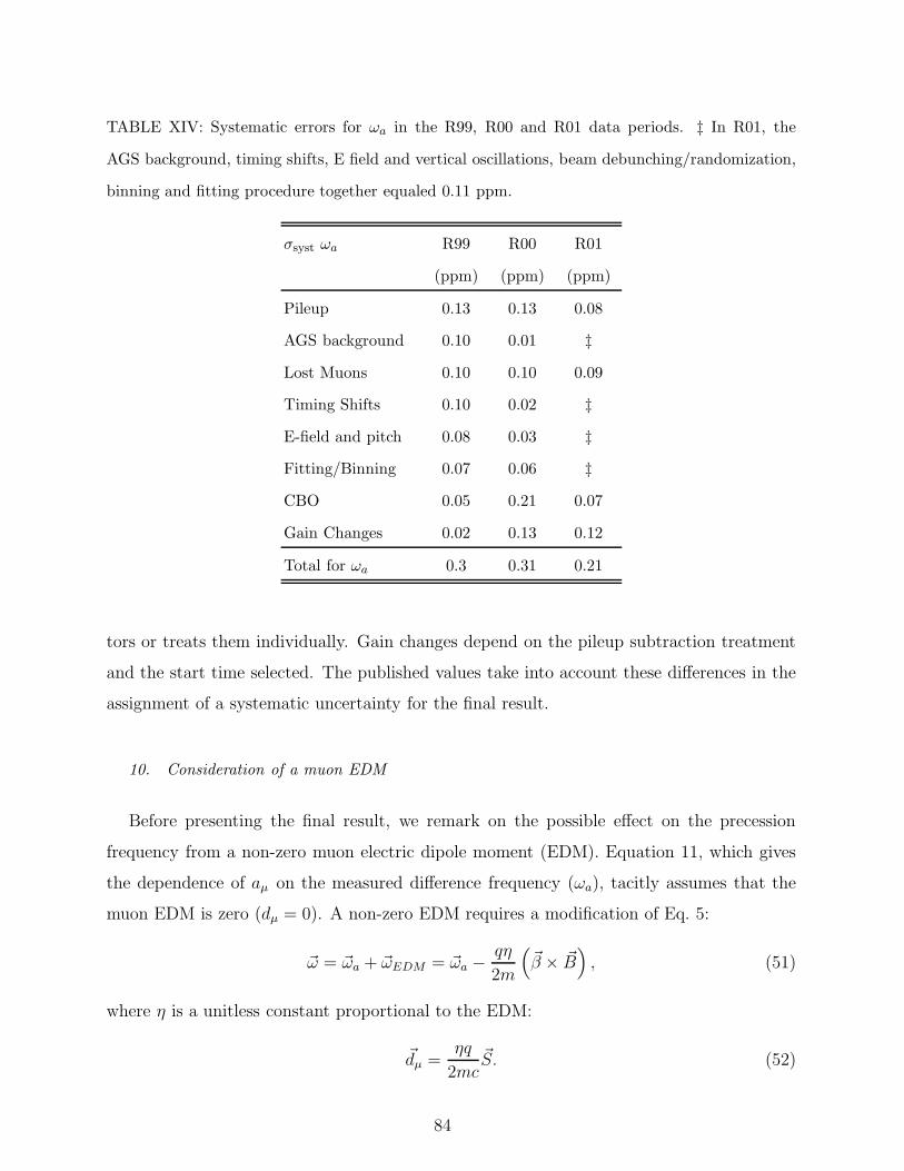
TABLE XIV: Systematic errors for ωa in the R99, R00 and R01 data periods. ‡ In R01, the
AGS background, timing shifts, E field and vertical oscillations, beam debunching/randomization,
binning and fitting procedure together equaled 0.11 ppm.
σsyst ωa R99 R00 R01
(ppm) (ppm) (ppm)
Pileup 0.13 0.13 0.08
AGS background 0.10 0.01 ‡
Lost Muons 0.10 0.10 0.09
Timing Shifts 0.10 0.02 ‡
E-field and pitch 0.08 0.03 ‡
Fitting/Binning 0.07 0.06 ‡
CBO 0.05 0.21 0.07
Gain Changes 0.02 0.13 0.12
Total for ωa 0.3 0.31 0.21
tors or treats them individually. Gain changes depend on the pileup subtraction treatment
and the start time selected. The published values take into account these differences in the
assignment of a systematic uncertainty for the final result.
10. Consideration of a muon EDM
Before presenting the final result, we remark on the possible effect on the precession
frequency from a non-zero muon electric dipole moment (EDM). Equation 11, which gives
the dependence of aµ on the measured difference frequency (ωa), tacitly assumes that the
muon EDM is zero (dµ = 0). A non-zero EDM requires a modification of Eq. 5:
~ω = ~ωa + ~ωEDM = ~ωa −qη
2m
(~β × ~B
), (51)
where η is a unitless constant proportional to the EDM:
~dµ =ηq
2mc~S. (52)
84
The interaction of the EDM with the motional electric field (in the muon rest frame)
induces a radial component in the spin precession vector, which is otherwise purely vertical.
The spin precession plane is tilted radially by angle δ:
δ ≈ η
2aµ
=dµ
1.1 × 10⁻¹⁶ e cm. (53)
Independent of its sign, an EDM increases the measured precession frequency,
ωmeas = ωa
√1 + δ2. (54)
A precession plane tilt causes an oscillation at ωmeas in the vertical direction of the decay
electrons and thus in the mean vertical position at the calorimeters. The vertical oscillation
reaches extrema when the spin points inward or outward radially, 90 out of phase with the
usual (g − 2) oscillation.
The vertical electron hit distribution on the FSDs was examined for oscillations having
this phase relation. Additionally, the traceback wire chambers were used to look for oscilla-
tions in the vertical decay angle of the electrons. Both methods find null results. The final
analysis of the EDM studies from our experiment is being completed and we expect to achieve
a limit of a few times 10−19 e cm. The details will be described in a separate paper [41].
However, to set the scale of the potential effect, a non-zero EDM at 2.0 × 10⁻¹⁹e cm would
cause a systematic increase to aµ by 1.6 ppm. A more sensitive limit is obtained by invoking
muon-electron universality and the linear scaling relation expected for many standard model
extensions: dµ ≈ (mµ/me)de. With the current electron EDM limit, de < 1.6 × 10⁻²⁷ e cm,
linear scaling implies a muon upper limit below 3.2 × 10⁻²⁵ e cm. An EDM of this mag-
nitude is too small to affect the ωa measured in this experiment. Therefore, we adopt the
assumption that the measured anomalous precession frequency alone determines aµ .
C. Final aµ result
The final aµ result is obtained by combining the individual aµ results from all running
periods, which are listed in Table I. All E821 results are plotted in Figure 40 together with
the final average.
Recall that the relation
aµ =R
λ−R
85
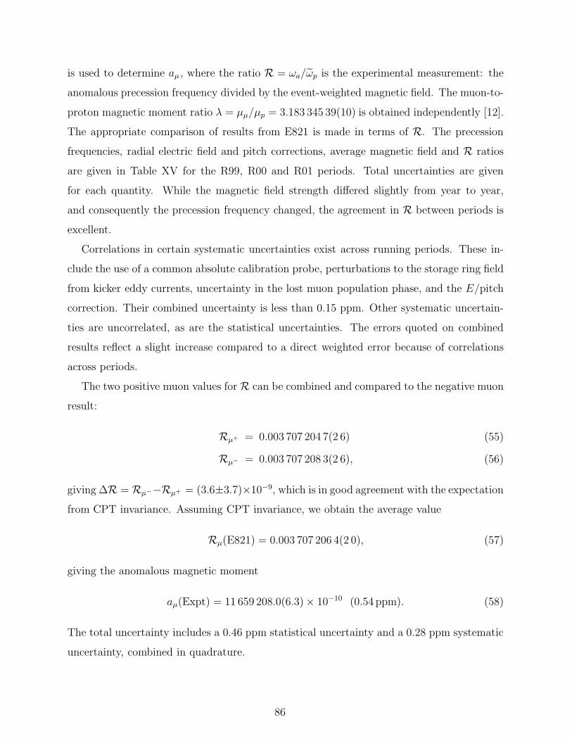
is used to determine aµ , where the ratio R = ωa/ωp is the experimental measurement: the
anomalous precession frequency divided by the event-weighted magnetic field. The muon-to-
proton magnetic moment ratio λ = µµ/µp = 3.183 345 39(10) is obtained independently [12].
The appropriate comparison of results from E821 is made in terms of R. The precession
frequencies, radial electric field and pitch corrections, average magnetic field and R ratios
are given in Table XV for the R99, R00 and R01 periods. Total uncertainties are given
for each quantity. While the magnetic field strength differed slightly from year to year,
and consequently the precession frequency changed, the agreement in R between periods is
excellent.
Correlations in certain systematic uncertainties exist across running periods. These in-
clude the use of a common absolute calibration probe, perturbations to the storage ring field
from kicker eddy currents, uncertainty in the lost muon population phase, and the E/pitch
correction. Their combined uncertainty is less than 0.15 ppm. Other systematic uncertain-
ties are uncorrelated, as are the statistical uncertainties. The errors quoted on combined
results reflect a slight increase compared to a direct weighted error because of correlations
across periods.
The two positive muon values for R can be combined and compared to the negative muon
result:
Rµ+ = 0.003 707 204 7(2 6) (55)
Rµ− = 0.003 707 208 3(2 6), (56)
giving ∆R = Rµ−−Rµ+ = (3.6±3.7)×10−9, which is in good agreement with the expectation
from CPT invariance. Assuming CPT invariance, we obtain the average value
Rµ(E821) = 0.003 707 206 4(2 0), (57)
giving the anomalous magnetic moment
aµ(Expt) = 11 659 208.0(6.3)× 10−10 (0.54 ppm). (58)
The total uncertainty includes a 0.46 ppm statistical uncertainty and a 0.28 ppm systematic
uncertainty, combined in quadrature.
86
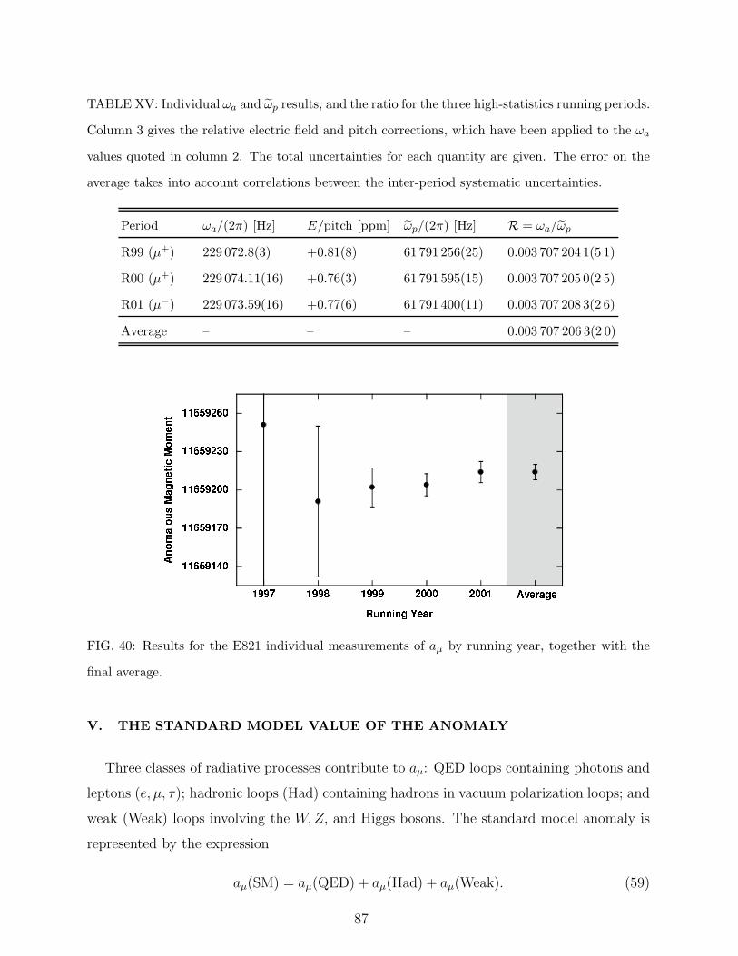
TABLE XV: Individual ωa and ωp results, and the ratio for the three high-statistics running periods.
Column 3 gives the relative electric field and pitch corrections, which have been applied to the ωa
values quoted in column 2. The total uncertainties for each quantity are given. The error on the
average takes into account correlations between the inter-period systematic uncertainties.
Period ωa/(2π) [Hz] E/pitch [ppm] ωp/(2π) [Hz] R = ωa/ωp
R99 (µ+) 229 072.8(3) +0.81(8) 61 791 256(25) 0.003 707 204 1(5 1)
R00 (µ+) 229 074.11(16) +0.76(3) 61 791 595(15) 0.003 707 205 0(2 5)
R01 (µ−) 229 073.59(16) +0.77(6) 61 791 400(11) 0.003 707 208 3(2 6)
Average – – – 0.003 707 206 3(2 0)
FIG. 40: Results for the E821 individual measurements of aµ by running year, together with the
final average.
V. THE STANDARD MODEL VALUE OF THE ANOMALY
Three classes of radiative processes contribute to aµ: QED loops containing photons and
leptons (e, µ, τ); hadronic loops (Had) containing hadrons in vacuum polarization loops; and
weak (Weak) loops involving the W,Z, and Higgs bosons. The standard model anomaly is
represented by the expression
aµ(SM) = aµ(QED) + aµ(Had) + aµ(Weak). (59)
87
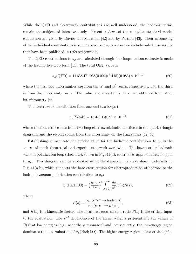
While the QED and electroweak contributions are well understood, the hadronic terms
remain the subject of intensive study. Recent reviews of the complete standard model
calculation are given by Davier and Marciano [42] and by Passera [43]. Their accounting
of the individual contributions is summarized below; however, we include only those results
that have been published in refereed journals.
The QED contributions to aµ are calculated through four loops and an estimate is made
of the leading five-loop term [44]. The total QED value is
aµ(QED) = 11 658 471.958(0.002)(0.115)(0.085)× 10−10 (60)
where the first two uncertainties are from the α4 and α5 terms, respectively, and the third
is from the uncertainty on α. The value and uncertainty on α are obtained from atom
interferometry [44].
The electroweak contribution from one and two loops is
aµ(Weak) = 15.4(0.1)(0.2) × 10−10 (61)
where the first error comes from two-loop electroweak hadronic effects in the quark triangle
diagrams and the second comes from the uncertainty on the Higgs mass [42, 45].
Establishing an accurate and precise value for the hadronic contributions to aµ is the
source of much theoretical and experimental work worldwide. The lowest-order hadronic
vacuum polarization loop (Had; LO), shown in Fig. 41(a), contributes approximately 60 ppm
to aµ . This diagram can be evaluated using the dispersion relation shown pictorially in
Fig. 41(a-b), which connects the bare cross section for electroproduction of hadrons to the
hadronic vacuum polarization contribution to aµ :
aµ(Had; LO) =(αmµ
3π
)2∫ ∞
4m2π
ds
s2K(s)R(s), (62)
where
R(s) ≡ σtot(e+e− → hadrons)
σtot(e+e− → µ+µ−), (63)
and K(s) is a kinematic factor. The measured cross section ratio R(s) is the critical input
to the evaluation. The s−2 dependence of the kernel weights preferentially the values of
R(s) at low energies (e.g., near the ρ resonance) and, consequently, the low-energy region
dominates the determination of aµ(Had; LO). The higher-energy region is less critical [46].
88
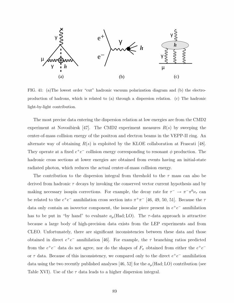
(c)(b)(a)
γ
µh
γ
−e
+e
h
γ
h
µ
γ
γ
FIG. 41: (a)The lowest order “cut” hadronic vacuum polarization diagram and (b) the electro-
production of hadrons, which is related to (a) through a dispersion relation. (c) The hadronic
light-by-light contribution.
The most precise data entering the dispersion relation at low energies are from the CMD2
experiment at Novosibirsk [47]. The CMD2 experiment measures R(s) by sweeping the
center-of-mass collision energy of the positron and electron beams in the VEPP-II ring. An
alternate way of obtaining R(s) is exploited by the KLOE collaboration at Frascati [48].
They operate at a fixed e+e− collision energy corresponding to resonant φ production. The
hadronic cross sections at lower energies are obtained from events having an initial-state
radiated photon, which reduces the actual center-of-mass collision energy.
The contribution to the dispersion integral from threshold to the τ mass can also be
derived from hadronic τ decays by invoking the conserved vector current hypothesis and by
making necessary isospin corrections. For example, the decay rate for τ− → π−π0ντ can
be related to the e+e− annihilation cross section into π+π− [46, 49, 50, 51]. Because the τ
data only contain an isovector component, the isoscalar piece present in e+e− annihilation
has to be put in “by hand” to evaluate aµ(Had; LO). The τ -data approach is attractive
because a large body of high-precision data exists from the LEP experiments and from
CLEO. Unfortunately, there are significant inconsistencies between these data and those
obtained in direct e+e− annihilation [46]. For example, the τ branching ratios predicted
from the e+e− data do not agree, nor do the shapes of Fπ obtained from either the e+e−
or τ data. Because of this inconsistency, we compared only to the direct e+e− annihilation
data using the two recently published analyses [46, 52] for the aµ(Had; LO) contribution (see
Table XVI). Use of the τ data leads to a higher dispersion integral.
89
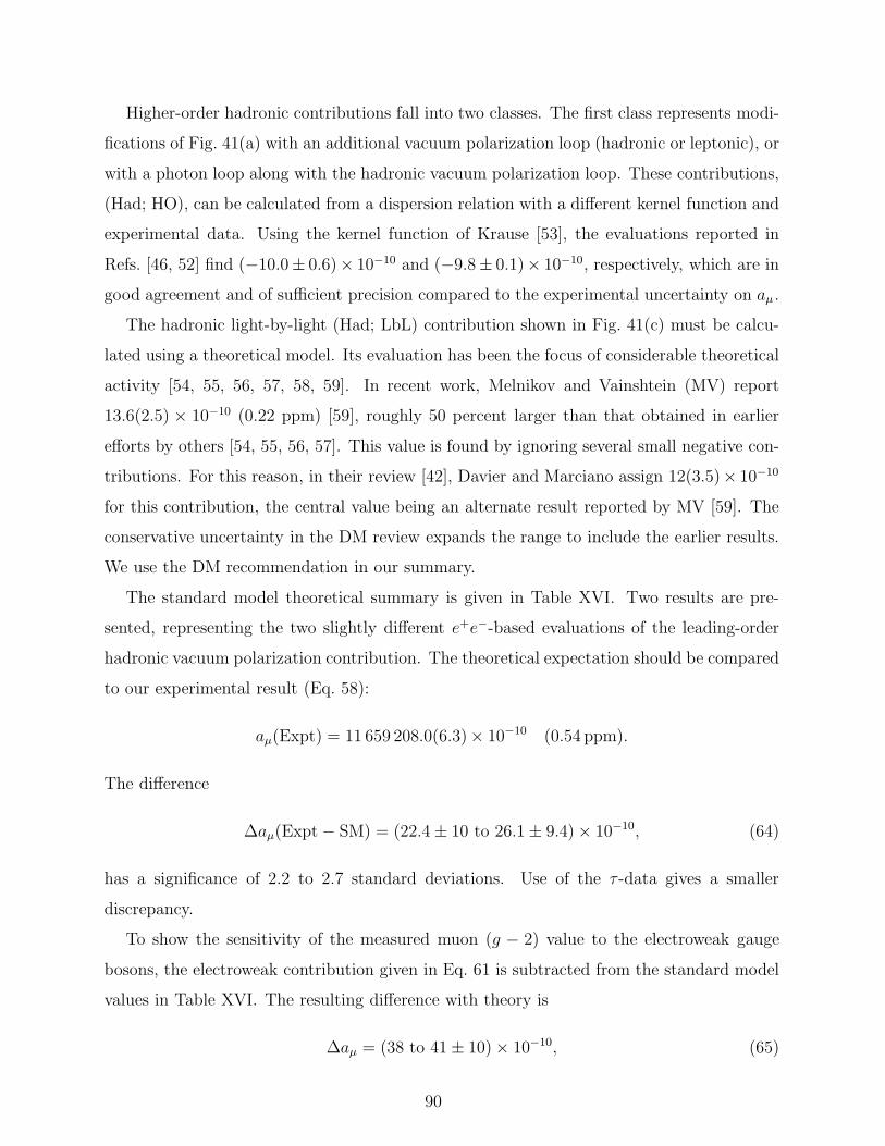
Higher-order hadronic contributions fall into two classes. The first class represents modi-
fications of Fig. 41(a) with an additional vacuum polarization loop (hadronic or leptonic), or
with a photon loop along with the hadronic vacuum polarization loop. These contributions,
(Had; HO), can be calculated from a dispersion relation with a different kernel function and
experimental data. Using the kernel function of Krause [53], the evaluations reported in
Refs. [46, 52] find (−10.0± 0.6)× 10−10 and (−9.8± 0.1)× 10−10, respectively, which are in
good agreement and of sufficient precision compared to the experimental uncertainty on aµ .
The hadronic light-by-light (Had; LbL) contribution shown in Fig. 41(c) must be calcu-
lated using a theoretical model. Its evaluation has been the focus of considerable theoretical
activity [54, 55, 56, 57, 58, 59]. In recent work, Melnikov and Vainshtein (MV) report
13.6(2.5) × 10−10 (0.22 ppm) [59], roughly 50 percent larger than that obtained in earlier
efforts by others [54, 55, 56, 57]. This value is found by ignoring several small negative con-
tributions. For this reason, in their review [42], Davier and Marciano assign 12(3.5)× 10−10
for this contribution, the central value being an alternate result reported by MV [59]. The
conservative uncertainty in the DM review expands the range to include the earlier results.
We use the DM recommendation in our summary.
The standard model theoretical summary is given in Table XVI. Two results are pre-
sented, representing the two slightly different e+e−-based evaluations of the leading-order
hadronic vacuum polarization contribution. The theoretical expectation should be compared
to our experimental result (Eq. 58):
aµ(Expt) = 11 659 208.0(6.3)× 10−10 (0.54 ppm).
The difference
∆aµ(Expt − SM) = (22.4 ± 10 to 26.1 ± 9.4) × 10−10, (64)
has a significance of 2.2 to 2.7 standard deviations. Use of the τ -data gives a smaller
discrepancy.
To show the sensitivity of the measured muon (g − 2) value to the electroweak gauge
bosons, the electroweak contribution given in Eq. 61 is subtracted from the standard model
values in Table XVI. The resulting difference with theory is
∆aµ = (38 to 41 ± 10) × 10−10, (65)
90
TABLE XVI: Contributions to the standard model value for aµ. The error in ppm refers to the
full value of aµ. The errors listed for (Had; LO) are the quadrature of those from the data and
from radiative corrections. The higher-order hadronic contribution does not include the hadronic
light-by-light term, which is listed separately. In computing the total, the higher-order hadronic is
taken from the same reference as the lowest-order hadronic.
Contribution Value Error Error Reference
[10−10] [ppm]
QED 11 658 471.958 0.143 0.012 [44]
Had; LO 696.3 7.2 0.62 [46]
Had; LO 692.4 6.4 0.55 [52]
Had; HO -10.0 0.6 0.05 [46]
Had; HO -9.8 0.1 0.01 [52]
Had; LBL 12 3.5 0.3 [42]
Weak 15.4 0.22 0.02 [42]
Total 11 659 185.7 8.0 0.69 [46]
11 659 182.0 7.3 0.62 [52]
or a 3.7 to 4.3 standard deviation discrepancy when the electroweak contribution is left out.
The standard model value of the muon’s magnetic anomaly is entirely the result of radia-
tive corrections from intermediate states formed from a wide range of known particles. It
is also sensitive to speculative effects beyond the standard model such as additional gauge
bosons, muon or gauge boson substructure or the existence of extra dimensions. Its value
is potentially quite sensitive to the presence of as yet undiscovered particles associated with
many generic manifestations of supersymmetry [42, 60].
VI. DISCUSSION AND CONCLUSIONS
Experiment E821 at Brookhaven is formally complete. All of the data are analyzed
for aµ and these independent muon anomalous magnetic moment evaluations have been
reported [8, 9, 10]. Our combined result—based on nearly equal samples of positive and
negative muons—represents a 14-fold improvement on the CERN-III experiment [5] of the
91
mid-1970’s. Our final measurement uncertainty is 0.54 ppm, corresponding to 0.46 ppm
statistical and 0.28 ppm systematic uncertainties, respectively. The magnetic field and
muon spin precession systematics are combined. The experimental promise and progress
since the proposal submission in 1984 motivated a significant theoretical effort to accurately
predict the standard model expectation for the muon anomaly. The theoretical uncertainty,
now 0.62− 0.69 ppm, has been reduced by more than an order of magnitude over the same
period. The difference between the measured and theoretical values, (22 − 26) × 10−10, lies
within the expected range for many standard model extensions.
Our (g − 2) Collaboration published individual results from the yearly running periods
and these were compared to the most up-to-date theory expectations. Improvements in the
theoretical calculations, new input data for the hadronic vacuum polarization analysis, and
corrections to the theory changed the standard model central value appreciably over this time
period. For example, the theoretical values quoted in Table XVI are higher by ∼ 24× 10−10
than the theory value quoted for our R99 result [8]. The dominant theoretical uncertainty is
associated with the leading-order hadronic vacuum polarization. Further work is in progress
at Novosibirsk, and additional data from both the CMD2 and SND experiments there will
be published in the near future. The B factories at SLAC and KEK are also using initial-
state radiation to measure R(s), and results should be forthcoming. Continued theoretical
modelling of the hadronic light-by-light contribution can also be expected, and initial studies
using the lattice have begun [61]. We are confident that the precision on the standard model
value will be improved, enabling a more sensitive comparison to experiment.
Because our measurement precision was ultimately limited by statistics, the question
naturally arises whether the current technique can be extended using a more intense muon
source. We have studied this question and have outlined a plan [62] that can reduce the
present uncertainty on aµ by a factor of 2.5 (or more), to a relative precision of ±0.2 ppm.
The effort requires straight-forward improvements in the magnetic field uniformity and map-
ping system and a five-fold increase in the muon production and storage rate. An important
feature of the design is the use of a “backward” decay beam to eliminate the hadronic-induced
flash. Other improvements are associated with increasing the muon transmission fraction,
optimizing the kicker efficiency, and replacing the detectors with segmented calorimeters
having independent readout digitizers.
Historically, precision tests of the standard model have led to both discoveries and refine-
92
ments in the predictive power of the theory. The series of CERN and BNL muon (g − 2)
experiments—spanning more than 40 years—has methodically progressed such that the
muon anomaly is now measured to sub-ppm precision. Over the same time, the standard
model theoretical development has progressed, with QED loops evaluated through fourth
order and estimated through fifth, weak loops through second order order, and hadronic
loops through second order. Many standard model extensions—SUSY is just one example—
suggest leading-order loops that will affect aµ at the ∼ 1 ppm (or slightly smaller) range.
The present sensitivity of the muon anomaly test of the standard model is ±0.9 ppm, with
roughly equal contributions from theory and experiment. Theory uncertainty improvement
can be expected from new experimental input for the hadronic contribution and from new
calculational approaches for the hadronic light-by-light term. We have described an approach
to improve the experiment uncertainty on the anomaly to ±0.2 ppm. Thus, we may expect
a significantly improved sensitivity for the anomaly test in the future. In the era of the LHC
and direct searches for specific standard model extensions, precision measurements, such as
that of the muon anomaly, represent a continually improving sum rule of known physics and
provide independent insight into physics at high energies and short-distance scales.
VII. ACKNOWLEDGMENTS
Many people have made important contributions towards the success of E821 over the
past twenty years when this experiment was proposed, built and completed. We thank N.P.
Samios, R. Palmer, R.K. Adair, T.L. Trueman, M. Schwartz, T.B.W. Kirk, P.D. Bond, M.
Murtagh†, S. Aronson, D.I. Lowenstein, P. Pile and the staff of the BNL AGS for the strong
support they have given; H. Hirabayashi and S. Kurokawa for their support of the magnet
technology provided by KEK; J.M. Bailey, J.R. Blackburn, W. Earle, M.A. Green, E. Hazen,
K. Ishida, J. Jackson, L. Jia, D. Loomba, W.P. Lysenko, J. Ouyang, W.B. Sampson, R.T.
Sanders, and K. Woodle for their contributions to parts of the preparation and running of the
experiment; J. Cullen†, C. Pai, C. Pearson, I. Polk; L. Snydstrup, J. Benante, D. von Lintig
and S. Kochis, who played major roles in the design and construction of the experiment.
We gratefully acknowledge M. Tanaka† for his development of the AGS extraction system
required for our experiment. We thank U. Haeberlen for his contributions to the development
of the NMR magnetometer system. We thank our colleagues J. Bijnens, A. Czarnecki,
93
M. Davier, E. de Rafael, S.I. Eidelman, A. Hocker, F. Jegerlehner, T. Kinoshita and W.
Marciano for very useful discussions on the theory.
We gratefully acknowledge L.M. Barkov for establishing the collaboration between the
Budker Institute and E821, both at BNL and on the R(s) measurements at BINP. W.W.
Williams† (U. Michigan) made important contributions in the early phases of this work and
in the development of the collaboration.
This work was supported in part by the U.S. Department of Energy, the U.S. National
Science Foundation, the German Bundesminister fur Bildung und Forschung, the Russian
Ministry of Science, the US-Japan Agreement in High Energy Physics, the NATO Office of
Scientific Research, and the U.S. National Computational Science Alliance. M. Deile, R.
Prigl and A. Steinmetz acknowledge support by the Alexander von Humboldt Foundation.
F.E. Gray was supported in part by a General Electric Fellowship, and C.S. Ozben by
the Scientific and Research Council of Turkey (TUBITAK). D.W. Hertzog acknowledges
partial support from the John Simon Guggenheim Foundation during the writing of this
manuscript.
[1] J. Schwinger, Phys. Rev. 73, 416 (1948).
[2] G. Charpak, F.J.M. Farley, R.L. Garwin, T. Muller, J.C. Sens, and A. Zichichi, Phys. Lett.
1, 16 (1962).
[3] J. Bailey et al., Nuovo Cimento A9, 369 (1972).
[4] J. Aldins, S.J. Brodsky, A.J. Dufner and T. Kinoshita, Phys. Rev. D 1, 2378 (1970).
[5] J. Bailey et al., Nucl. Phys. B150, 1 (1979).
[6] The g − 2 Collaboration: R.M. Carey et al., Phys. Rev. Lett. 82, 1632 (1999).
[7] The g − 2 Collaboration: H.N. Brown et al., Phys. Rev. D 62, 091101 (2000).
[8] The g − 2 Collaboration: H.N. Brown et al., Phys. Rev. Lett. 86, 2227 (2001).
[9] The g − 2 Collaboration: G.W. Bennett et al., Phys. Rev. Lett. 89, 101804 (2002); Erratum-
ibid. 89, 129903 (2002).
[10] The g − 2 Collaboration: G.W. Bennett et al., Phys. Rev. Lett. 92, 161802 (2004).
[11] E.J. Konopinski, Ann. Rev. Nucl. Sci. 9, 99 (1959).
[12] W. Liu et al., Phys. Rev. Lett. 82, 711 (1999).
94
[13] The Particle Data Group: D.E. Groom et al., The European Physical Journal C15, 1 (2000).
[14] S. O’Day, F. Bieniosek and K. Anderson, New Target Results from the FNAL Antiproton
Source IEEE 1993 Part. Acc. Conf., vol. 4, 3096 (1993).
[15] BTRAF, J. Sandweiss et al., BNL Bubble Chamber Group Report H-11 (1962), with additions
by H. N. Brown (1982) and A. S. Carroll (1983).
[16] A. Yamamoto et al., Nucl. Instrum. Meth. A491, 23 (2002).
[17] Frank Krienen, Dinesh Loomba and Wuzheng Meng, Nucl. Instrum. Meth. A283, 5 (1989).
[18] G.T. Danby et al., Nucl. Instrum. Meth. A457, 151 (2001).
[19] Y.K. Semertzidis et al., Nucl. Instrum. Meth. A503, 458 (2003).
[20] E. Efstathiadis et al, Nucl. Instrum. Meth. A496, 8 (2002).
[21] OPERA, Electromagnetic Fields Analysis Program, Vector Fields Ltd., 24 Bankside, Oxford
OX5 1JE, England.
[22] R. Prigl et al., Nucl. Instrum. and Meth. A374, 118 (1996).
[23] W.D. Phillips et al., Metrologia 13, 179 (1979).
[24] Superintendent of Documents, LORAN-C User’s Handbook, U.S. Government Printing Office
#050-012-00331-9, 1992.
[25] S.A. Sedykh et al., Nucl. Instrum. Meth. A455, 346 (2000).
[26] J. Ouyang, et al., Nucl. Instrum. Meth. A374, 215 (1996).
[27] M. Sossong et al., Traceback wire chamber system for the muon g-2 experiment, submitted to
Nucl. Instrum. Meth., March 10, 2005.
[28] Helmut Wiedemann, Particle Accelerator Physics, V1, Springer-Verlag, 1993.
[29] F. Combley and E. Picasso, Phys. Reports C14, 1 (1974).
[30] F.J.M. Farley, Phys. Lett. 42, 66 (1972).
[31] Jackson JD. Classical Electrodynamics, pp. 556-560, John Wiley & Sons Inc. (1975).
[32] X. Fei, V.W. Hughes, and R. Prigl, Nucl. Instrum. Meth. A394, 349 (1997).
[33] P.J. Mohr and B.H. Taylor, Rev. Mod. Phys. 77, 1 (2005).
[34] P.F. Winkler, D. Kleppner, T. Myint, and F.G. Walther, Phys. Rev. A5, 83 (1972).
[35] W.E. Lamb Jr., Phys. Rev. 60, 817 (1941).
[36] H. Grotch and R.A. Hegstrom, Phys. Rev. A 4, 59 (1971).
[37] B.W. Petley et al., Metrologia 20, 81 (1984).
[38] V.W. Hughes, in Physics Since Parity Symmetry Breaking, ed. Fan Wang, World Scientific,
95
Singapore, 508 (1999).
[39] S.I. Redin et al., Nucl. Instrum. Meth. A473, 260 (2001).
[40] Detector #2 is missing due to a hardware malfunction and station #20 is the traceback station.
[41] The g − 2 Collaboration, in preparation.
[42] M. Davier and W. Marciano, Ann. Rev. Nucl. Part. Sci. 54, 115 (2004).
[43] M. Passera, J. Phys. G31, R75 (2005).
[44] T. Kinoshita and M. Nio, Phys. Rev. Lett. 90, 021803 (2003); Phys. Rev. D 70, 113001 (2004).
[45] W.A. Bardeen, R. Gastmans and B Lautrup, Nucl. Phys. B46, 319 (1972); R. Jackiw and S.
Weinberg, Phys. Rev. D 5, 157 (1972); I. Bars and M. Yoshimura, Phys. Rev. D 6, 374 (1972);
A. Czarnecki, B. Krause and W.J. Marciano, Phys. Rev. D 52, R2619 (1995); S. Peris, M.
Perrottet and E. de Rafael, Phys. Lett. B355, 523 (1995); A. Czarnecki, B. Krause and W.J.
Marciano, Phys. Rev. Lett. 76, 3267 (1996); G. Degrassi and G.F. Giudice, Phys. Rev. D 58,
53007 (1998); Marc Knecht, Santiago Peris, Michel Perrottet, Eduardo De Rafael, JHEP 11,
003 (2002); A.Czarnecki, W.J. Marciano, A. Vainshtein, Phys. Rev. D 67, 073006 (2003).
[46] M. Davier, S. Eidelman, A. Hocker, and Z. Zhang, Eur. Phys. J. C31, 503 (2003).
[47] R.R. Akhmetshin, et al, CMD2 collaboration, Phys. Lett. B578, 285 (2004).
[48] A. Aloisio, et al., KLOE Collaboration, Phys. Lett. B606, 12 (2005).
[49] M. Davier, S. Eidelman, A. Hocker, and Z. Zhang, Eur. Phys J. C27, 497 (2003).
[50] R. Alemany, M. Davier and A. Hocker, Eur. Phys. J. C2, 123 (1998).
[51] M. Davier and A. Hocker, Phys. Lett. B435, 427 (1998).
[52] K. Hagiwara, A.D. Martin, Daisuke Nomura, and T. Teubner, Phys. Lett. B557, 69 (2003);
Phys. Rev. D 69, 093003 (2004).
[53] Bernd Krause, Phys. Lett. B390, 392 (1997).
[54] Johan Bijnens, Elisabetta Pallante and Joaquim Prades, Phys. Rev. Lett. 75, 1447 (1995);
Phys. Rev. Lett. 75, 3781 (1995); Nucl. Phys. B474, 379 (1996); Nucl. Phys. B626, 410
(2002).
[55] M. Hayakawa and T. Kinoshita Phys. Rev. D 57, 465 (1998); and KEK-TH-793 (2001).
[56] Marc Knecht, Andreas Nyffeler, Phys. Rev. D 65, 073034 (2002).
[57] M. Knecht, A. Nyffeler, M. Perrottet, E. deRafael, Phys. Rev. Lett. 88, 071802 (2002).
[58] I. Blokland, A. Czarnecki and K. Melnikov Phys. Rev. Lett. 88, 071803 (2002).
[59] K. Melnikov and A. Vainshtein, Phys. Rev. D 70, 113006 (2004).
96

[60] Andrzej Czarnecki and William J. Marciano, Phys. Rev. D 64, 013014 (2001).
[61] T. Blum, Phys. Rev. Lett. 91, 052001 (2003).
[62] New (g-2) Collaboration: R.M. Carey, et al., A (g-2) Experiment to 0.2 ppm Precision, BNL
P969, (2004).
97