]:, •

/

-..,./, /3)7

Final Report

NASA Ames Cooperative Agreement. NCC 2-357

Report for the period Oct 1985 to Sept 1989

by

Dr. Sreedhara V. Murthy

Principal Investigator: Dr. Sreedhara V. Murthy

Recipient Institution: University of the Pacific(Dept of Mechanical Engineering)3601, Pacific Ave, Stockton, CA 95211

https://ntrs.nasa.gov/search.jsp?R=19900015241 2018-05-28T02:02:58+00:00Z

Final Report

NASA Ames Co-op Agreement No. NCC 2-357

Report for the period October 1985 to September 1989

by

Dr. Sreedhara V. Murthy

Flow Unsteadiness Effects on Boundary Layers

Principal Investigator:

Recipient Institution:

D-r:-S-r-e-edh-ara V. Mt}rthy

University of the Pacific

(Department of Mechanical Engineering)

3601, Pacific Avenue, Stockton, CA 95211

Submitted to: Dr. Frank W. Steinle

Chief, Aerodynamic Facilities Branch Code RAF

NASA Ames Research Center, Moffett Field, CA 94035

Copy to: NASA Scientific and Technical Information Facility

P.O. Box 8757

Baltimore/Washington International Airport, Maryland 21240

Overall Objectives

University and Ames personnel would collaborate on performance of research to develop qual-

itative and quantitative understanding of the development of boundary layers at high subsonic

speeds in the presence of either mass flux fluctuations or acoustic disturbances or both.

Final Report for Co-op Agreement No. NCC 2-357, Oct. 1989 2

Contents

1 Background 3

2 Review of Existing Literature 4

3 Apparatus for Experiments 8

4 Instrumentation- Buried Wire Gages

4.1

4.2

4.3

4.4

4.5

4.6

4.7

4.8

9

General Aspects of Buried Wire Gage Technique .................. 9

Fabrication of Buried Wire Gages ........................... 10

Calibration Law for Buried Wire Gages ....................... 11

Data Reduction Method for Pipe-flow-based Calibrations ............. 12

4.4.1 Pipe-flow Profile Definitions ......................... 14

4.4.2 Pipe-flow Governing Equations ........................ 14

4.4.3 Pipe-flow Profile Properties .......................... 15

4.4.4 Pipe-flow Experiments and Validation of Data Reduction Method .... 16

Apparatus for flow-Calibration of Buried Wire Gages ............... 18

Flow Calibration of Buried Wire Gages ....................... 18

Buried Wire Gage Calibration Checks ........................ 19

Calibration Constants of Typical Buried Wire Gages ................ 19

Instrumentation- Hot Wire Probes, Transducers, etc. 20

5.1 Hot Wire Probes .................................... 20

5.2 Pressure Transducers .................................. 20

5.3 Data System ...................................... 20

6 Experiments 21

6.1 Preparation for Experiments ............................. 21

6.2 Measurements, Results and Discussion ........................ 25

7 Concluding Remarks 27

8 List of Publications 29

Final Report for Co-op Agreement No. NCC 2-357, Oct. 1989 3

1 Background

The research tasks identified in this Co-operative Agreement emerged from the need to generate

new inputs to the design database of advanced technology concepts such as advanced aircraft

wing shapes, special types of rotorcraft aerodynamic configurations, and Laminar Flow Con-

trol techniques. The inputs from the project were to be in the subject area of boundary layer

transition and growth at high subsonic and transonic flow speeds, particularly relating to the

effects of freestream mass flux fluctuations and acoustic disturbances (the two most important

parameters in the flow unsteadiness environment affecting the aerodynamics of a flight vehicle).

Existing knowledge in this area was rather limited in terms of both computational prediction

techniques and wind tunnel data updating capabilities.

With regard to the computational techniques, the quantum advancement that has occurred

during the recent years in computational concepts could not be fully exploited for providing

the desired level of confidence in predicted aerodynamic data, primarily because of the absence

of a sufficiently detailed database that could inspire proper modeling of the transitional and

turbulent states of boundary layers. Also, there existed only very limited information on the

effects of many types of flow disturbances such as those generated by propulsive units, air in-

takes, protrusions, etc on the boundary layer developing over wing surfaces.

In contrast to this status on computational techniques, the situation with respect to wind tunnel

data application capabilities and correction methodologies was not very different. A moderate

level of understanding had been achieved, notably on the effects of tunnel wall interference,

model and support system blockage,etc, but very little was known about the individual effects

of free-stream flow-unsteadiness components, namely acoustic noise and turbulence, in the mea-

sured aerodynamic data.

The limitations in prediction capabilities and wind tunnel data updating procedures had meant

that the complement of flight testing in aerospace vehicle development programs would remain

almost prohibitively large. A better, high quality research database was needed to serve as a

basis for constructing and validating new improved computational techniques, and to evaluate

or update wind tunnel data application methodologies.

It was recognized that the new high quality research database must fully reflect the many

ways in which the wind tunnel flow environment differed from the flight environment. Basically

the difference between the two environments may be characterized by three flow quality parame-

ters: freestream turbulence, pressure fluctuations, and temperature spottiness. (see Fig-l). The

levels and spectra of these parameters would be related to the flow disturbance sources, namely,

fan rotation, flow turning at bends, wall boundary layer, wall geometry, and model support in the

case of wind tunnels, and gusty winds, temperature gradients, clear air turbulence, and influence

from other parts of aircraft, in the case of flight. Data from each wind tunnel corresponds to

a given combination of these parameters, as those exist in that tunnel. In order to apply this

data to a flight environment composed of a different combination of flow quality parameters or

to compare it with data from another wind tunnel, the best procedure was to apply corrections,

one step at time, to the data for the differences in each of the individual flow quality parameters.

To do so, it was essential to start from a database that provided the individual influences of

these parameters. Of primary interest was the database on boundary layer transition phenom-

Final Report for Co-op Agreement No. NCC 2-357, Oct. 1989 4

ena. Typically, with properly applied corrections, the location of transition would be correctly

predicted, and the rest of the fiowfield on a wing profile would also be adequately mapped

(see Fig.`2). A good, high quality database was therfore the key to successful predictions. The

present Co-operative Agreement research project was specially aimed at generating such a high

quality database, say, for generating detailed information concerning free-stream flow unsteadi-

ness effects on boundary layer growth and transition in high subsonic and transonic speed ranges.

In specific terms, the Co-operative Agreement was intended to generate the desired database

with a two-pronged approach: (i) from a detailed review of existing literature on research and

wind tunnel calibration database, and (ii) from detailed tests in a special apparatus, namely

the Boundary Layer Apparatus ]or Subsonic and Transonic flow Affected by Noise Environment,

('BLASTANE'), available at the Aerodynamics Division of NASA Ames Research Center. For

the tests in BLASTANE, special instrumentation, including hot wire anemometry, the buried

wire gage technique, and laser velocimetry, were to be used to obtain skin friction and turbu-

lent shear stress data all along the laminar, transitional and turbulent stages of boundary layer

growth, for various free-stream noise levels, turbulence content, and pressure gradients. This

data base would then be useful for improving the correction methodology of applying wind tun-

nel test data to flight predictions and further would be helpful in providing pointers for making

improvements in turbulence modeling laws.

2 Review of Existing Literature

Research literature relating to the results of recent investigations was reviewed in order to ob-

tain a better insight into the effects of different flow parameters on boundary layer transition

phenomena at high subsonic and transonic speeds.

With respect to the existing database, it was noted that, a series of detailed tests on the standard

'Ten-Degree Cone' in several major wind tunnels had provided many pointers to the effects of

flow unsteadiness levels in wind tunnels. A detailed review co-authored by the principal inves-

tigator showed that the existing database on the ten-degree cone did not fully clarify some of

the important questions pertaining to the effects of the different flow unsteadiness components

on boundary layer growth and transition phenomenon (see Publication Nos. 1 and '2). The

review pointed out that the data base presented only the combined effects of acoustic noise, its

frequency content, free-stream turbulence and Mach number, as those existed in the different

wind tunnels participating in the ten-degree cone database effort.

The review further revealed that scatter in the data did not permit firm conclusions about

the individual effects of the different flow variables. However, it was possible to propose new

correlations that could act as guidelines to further effort in this area.

The detailed review began with a look at the theoretical methods. Earlier researchers had de-

termined that the relationship between the so-called critical Reynolds number from infinitesimal

disturbance stability theory and the actual transition Reynolds number was weak quantitatively

and only moderately strong qualitatively. From the present author's view-point, this was to

Final Report for Co-op Agreement No. NCC 2-357, Oct. 1989 5

be expected because the stability theory can only give pointers to the prediction of point of

instability, but cannot provide a reliable basis for predictions of conditions further downstream

where the disturbances will have grown to levels that are typical to a turbulent state. It was

concluded that the existing theoretical methods need to be be updated, perhaps by first con-

structing new stability and disturbance-growth criteria, then validating those criteria in the

context of research data from experiments, and finally, incorporating such new criteria in the

boundary layer growth calculations. This meant that a new high quality experimental research

database, of the type contemplated in the present project, was a pre-requisite. In the meantime,

the principal investigator therfore decided to attempt new empirical correlations.

The methods used by earlier researchers for arriving at their conclusions seemed to indicate

that they had concentrated on correlations with pressure fluctuation level and unit Reynolds

number. The principal investigator reviewed the existing literature with a wider interpretation,

and was able to postulate some new thoughts with respect to the possibilities of other correla-

tions; say, with respect to the effect of Mach number, and the role of vorticity as an independent

parameter compared to acoustic disturbances. These thoughts were basically triggered by the

database from flight tests of the so-called standard AEDC Ten Degree Cone which was also sub-

ject to a series of detailed tests in many large wind tunnels (see Fig.3). Additional support to

these thoughts came by way of the data from some of the wind tunnels that had comparativelylow flow unsteadiness levels.

In order to postulate new correlations, the principal investigator attempted first to establish

an empirical correlation for the effects of Mach number alone, separate from other parameters

(vorticity and acoustic fluctuations).

Clearly, the entire database could not be used for the reason that much of the database had

significant influences of other flow parameters that affect the transition phenomena. Out of

the data base, a part that corresponded to relatively low levels of disturbance was extracted

and examined for Mach number correlation. Mach number of 0.8 was arbitrarily taken as the

reference Mach number. With respect to transition Reynolds number, the average of measured

transition Reynolds numbers at Mach 0.8 in a given facility was taken as the reference transition

Reynolds number for the data from that facility. The data was presented in a special format as

seen in the reproduced figure (see Fig.f) in this report. The format of the figure was chosen to

provide a convenient display of the Mach number trend for transition Reynolds numbers. Flight

data, as seen in the figure, was shown as an envelope (hatched area) because the number of

measurements is too large to reproduce individually. All the data in figure corresponded to low

levels of disturbance - low to the extent that the pressure fluctuation levels (ratio of root mean

square value of pressure fluctuations to the flow dynamic pressure) are less than one percent.

The choice of one percent, rather than a lower value was derived from the desire to have a

reasonably large sample of data. It was clear from the figure that both the beginning-of and the

end-of transition Reynolds numbers are affected by Mach number. Given the spread in the flight

data and the scatter in the wind tunnel test data, it was considered best to conclude that the

effect of Mach number on either the beginning-of or end-of transition Reynolds numbers could

be considered linear, with a correlation slope of 3 million per unit increment of Mach number.

Final Report for Co-op Agreement No. NCC 2-357, Oct. 1989 6

The following correlation between the beginning-of or end-of-transition Reynolds number,

Ret o_T, and Mach number, M, was thus evolved from the figure:

_Ret or T-3× 10 e

&M

This correlation formed the basis for defining an "Equivalent Transition Reynolds num-

ber", Re(t o, r),_q,i_ that related each data point at different Mach numbers to a reference Machnumber of 0.8.

Re(t o_ r),_qui_ = Ret o_ r._tM -- (M - 0.8) x 3 × 10 6

It was important to subtract the effect of Mach number in this manner before examining the

effects of flow disturbances because, for any desired Mach number, the existing database did

not provide a large enough sample to help evaluate the effects of flow disturbance levels. With

this thinking, it was possible to find new correlations with respect to the effects of pressure

fluctuations and freestream turbulence. It may be noted here that earlier researchers had at-

tempted correlations and come to the conclusion that both the beginning- and end-of-transition

Reynolds numbers were correlated with pressure fluctuation level. But, in the present review, it

was found that such a correlation was not quite satisfactory (see Fig.5). Once the effects of com-

pressibility were subtracted from the data through the definition of the Equivalent Transition

Reynolds Number, there seems to be no correlation at all for low noise levels, and no reliable

correlation for higher levels (see Fig.6).

Having thus established that there is no acceptable correlation for pressure fluctuations, the

next step was to examine the possibility of correlations with freestream turbulence.

Evidence of strong influence of free stream turbulence on boundary layers had been overwhelm-

ing. It was well known through extensive testing that an increase in the level of freestream

turbulence would cause an increase in the amplification rates of flow disturbances, thus has-

tening transition. Influence of freestream turbulence was known to be significant all through

the diffcrent stages of boundary layer (laminar, transitional, and turbulent). It was established

that, with higher freestream turbulence, stability of laminar boundary layer was substantially

reduced, onset of turbulence fluctuations in transition region was hastened, and skin friction

along with other properties of turbulent boundary layer were significantly altered. It was thus

very likely that freestream turbulence level would correlate well for transition Reynolds number.

A correlation plot was prepared for transition data from the wind tunnels for which freestream

turbulence data was available. It became readily clear that both the beginning- and end-of-

transition Reynolds numbers decreased with increasing freestream turbulence levels. The cor-

relation plot was constructed with Equivalent Transition Reynolds Numbers to properly isolate

the effects of Mach number (see Fig. 7). The correlation laws could be postulated as:

or U -nRe(t T),equiv Ot (p )rm,_

1 1

with n : -_ for beginning of transition, and n = -6 for end of transition

Final Report for Co-op AgreementNo. NCC 2-357, Oct. 1989 7

Another correlation could also be derived for the effects of freestream turbulence. The ratio

of beginning-of-transition to end-of-transition Reynolds numbers was related to freestream

turbulence, but only weakly (see Fig.8):

Ret,equiv 1_

ReT,eq=_v ct (pu)rrn,%

It was an important step in the Cooperative Agreement project, that the review of existing lit-

erature made it possible to postulate new correlations for the effects of flow quality parameters.

To further proceed and establish these new correlations, it was essential to obtain a better high

quality database so that the scatter in data would not be a subject of argument with regard to

the new correlation laws. The experimental part of the Cooperative Agreement was organized

to provide this high quality database.

One other aspect relating to the effect of flow unsteadiness became evident during a review

of the most recent flow measurements made in the NASA Ames 12 FT PWT entry-flow condi-

tioning chamber. It became known that the characteristics of flow quality in the wind tunnel

test section are dependent on a variety of factors, namely, the geometry of the bends, the turning

vanes, the Contraction ratio, and the specific type of flow conditioning elements installed in the

entry flow circuit. The influence of these factors appeared to be so varied that an appreciation

of the flowfield emerging from the each individual flow-conditioning-device would be desirable

in order to properly compose the full range of flow unsteadiness conditions that must be covered

in the proposed studies of boundary layer transition phenomena. In this context, it is important

to note that the unsteadiness in the flowfield emerging from the screens and honeycombs could

be accompanied by a variation in mean velocity, which could then break-up into a turbulence

field of its own, resulting in higher turbulence downstream. This would mean that standard

turbulence decay law cannot be applied to obtain turbulence level at different stations in a

wind tunnel test section, and therefore the turbulence field, in terms of intensity and isotropy,

will have to be documented through a series of special experiments for that type of situation.

Finally, the turbulence field entering a contraction is modified at the exit from contraction, but

the effects are not always monotonic with respect to the contraction ratio.

It was decided that some studies ought to be made with respect to the characteristics of turbu-

lence and velocity fields emerging from the different flow-conditioning devices commonly used in

wind tunnels. A similar database was also needed for the NASA-Ames 12 FT PWT Restoration

Project, and it was possible to combine the test requirements of the present research program

with the data-base requirements of the 12 FT PWT project in such a way as to perform a single

combined test program on a series of flow-conditioning elements.

Final Report for Co-op Agreement No. NCC 2-357, Oct. 1989

3 Apparatus for Experiments

The experimental part of the Cooperative Agreement was an important part of the overall goals,

and was organized with great care to provide a high quality database for the effects of flow

quality parameters on boundary layer transition phenomena. The idea was to further develop a

special apparatus, called Boundary Layer Apparatus for Subsonic and Transonic flows Affected

by Noise Environment ("BLASTANE'), to a stage where it could be used to generate a variable

flow environment suited to detailed studies on the effects of all the different parameters that

influence the transition phenomena. It was recognized that the the main purpose for developing

the apparatus (BLASTANE) was to establish a high quality database that would provide the

basis for constructing a new method of comparing and correlating data from different wind

tunnels and flight tests. In this regard, a critical requirement was that the apparatus must be

of the variable configuration type, and must, at one end of the operating envelope, provide a

very low flow unsteadiness level for base-line data generation. The apparatus would then be

configured to provide varying levels of the different flow quality variables namely, compressibility,

free-stream turbulence, pressure fluctuations, their frequency content, temperature spottiness,

and pressure gradient.

The development targets of the apparatus were identified as:

Apparatus Development Targets

• To obtain flow surface accuracy and surface finish typical to those of Wind Tunnel Models.

• To achieve Mach Number range of up to Mach-1, higher Mach nos. if possible.

• To generate Varying Flow Unsteadiness Levels:

- Acoustic Noise Level from Very Low to 3% in RMS Pressure Coeff.

- Frequency Content from 100 Hz to 2 KHz.

- Turbulence from Very Low to 3% RMS Mass Flux Fluctuations.

A brief description of the fully developed apparatus is given below:

The apparatus is very similar to a wind tunnel except for the one critical feature that the

Test Section wall surface itself is to serve as the flow surface of interest for boundary layer

studies and therefore had to be dimensionally very accurate and very smooth, typical to high

speed wind tunnel model surfaces (see Figs. 9, 10, 11). Flow is induced by a vacuum source

connected via a Diffuser section to the exit end of Test Section. The Diffuser has a diverging

taper and accommodates a smoothly contoured Flow Control Plug that can be traversed along

the centerline of the Diffuser to obtain different flow Mach numbers in the Test Section. For

any desired Mach number in the Test Section, the Plug setting in the diverging passage of the

Diffuser is so chosen as to ensure sonic "choking _ of flow at the maximum diameter station of

the plug, thus preventing any downstream disturbances from reaching the Test Section flow.

Quality of flow in the Test Section then depends entirely on the conditions upstream in the

Contraction section and the Settling Chamber.

Final Report for Co-op Agreement No. NCC 2-357, Oct. 1989 9

BLASTANE Apparatus - Brief Description

ITEM DESCRIPTION

Overall Type • vacuum driven wind tunnel, choked (sonic) exit flow from test section.

• long test section, smooth walls (low wall-induced disturbances)

Flow Speeds • Test Section Mach= up to 1.0, atmospheric stagnation.

Test Section • 10 inch din., 72 inch long, very smooth wall surface.

Contraction • 9:1

Settling Chamber • fitted with desired number of screens to obtain

variable turbulence levels.

fitted with an entry flange that can accommodate an electrically

excited speaker for producing variable pressure fluctuation levels.

Air Intake Chr. • fitted with filters to remove any contamination in entry air flow.

While performing preliminary tests to bring the BLASTANE apparatus to a fully operational

status, it had become clear that the acoustic noise level in the room was rather excessive, large

enough to cause a high pressure fluctuation level, in excess of 95 dBA, in the entry flow of the

apparatus. This would adversely affect the capability to generate a complete set of baseline

data on boundary layer flow for very low noise levels-- a limitation which could not be ac-

cepted. Steps were therefore taken to reduce the noise level. The pipes and the bellows in the

BLASTANE piping were wrapped with noise suppression material, and the noise level at the

entry end of the Air Intake Chamber was reduced to less-than 85 dBA.

4 Instrumentation- Buried Wire Gages

Instrumentation consisted of conventional types, such as wall static pressure taps with a scanning

transducer system, hot wire probes operated from constant temperature anemometer systems,

and flush-mounted high response dynamic pressure transducers (see Fig.12). In addition, be-

cause of the need to generate a high quality database in the apparatus, it was necessary to

develop special types of flow instrumentation to non-intrusively measure wall flow properties,

such as wall shear stress. One very promising technique was the "Buried Wire Gage" technique

which relied on the heated element concept for providing a measure of wall shear stress. The

development of this technique consisted of first making reliable gages, and then calibrating those

in a reliable flowfield. This development was a first-of-the-kind effort, and is described in the

following sections.

4.1 General Aspects of Buried Wire Gage Technique

Buried Wire Gage Technique is based on the heated element concept which was conceived several

decades ago; but, application of that concept in practical flow situations remained a formidable

problem for a long time because of the lack of a proper sensor that could provide an adequate

level of sensitivity.

Typically, the heated element concept consists of a sensing element that is arranged flush to

the wall surface in a flow (see Fig.13). The element is heated to an appropriate temperature so

that the characteristics of heat transferred to the wall layer of flow may be measured. However,

Final Report for Co-op Agreement No. NCC 2-357, Oct. 1989 10

the heat transferred to the wall-flow layer is only a part of the total heat transfer that can

be measured, namely the heat transferred away from the sensing element. The other part of

the measured heat transfer is what is lost by thermal conduction to the substrate material

surrounding the heated element. The proportion of heat transferred to the substrate material

could be rather large for most choices of conventional substrate materials such as pyrex, quartz,

plexiglas, etc, which are popularly used for "hot film" gages. With large losses to substrate,

the sensitivity of flow measurement will suffer. Therefore, it was considered important that a

proper choice be made for the substrate material.

Another aspect of the heated element concept that relies heavily on the characteristics of the

sensor is the streamwise extent of the sensing element in the flow. Part of the measured heat

transfer to wall layer of flow consists of the effects of local pressure gradients in the flow. These

effects must be properly accounted for before the component of measured heat transfer relating

solely to the wall flow friction may be extracted and converted to wall shear-stress. The pressure

gradient component was known to be proportional to the streamwise extent of the sensing

element and therefore could be reduced by making the sensing element appreciably slender.

The Buried Wire Gage technique seemed to satisfy both primary requirements: adaptability to

low conductivity substrate materials, and very small streamwise extent. The gage consists of

a very slender wire (a few microns in diameter) which is spot welded at its ends to a pair of

electrical leads that are flush-embedded on a low thermal conductivity substrate. The wire is

firmly attached to the substrate surface by a bonding process.

It was noted that the Buried Wire Gages are non-intrusive and readily provide a measure of the

wall flow skin friction. Also such gages were known to have calibrations that were independent

of the state of the boundary layer - laminar, transitional or turbulent.

4.2 Fabrication of Buried Wire Gages

The gages were developed specially to suit the instrument plugs that matched the test section

1 inch spac-walls of BLASTANE (see Fig.1._, 15). Each plug was to be equipped with 5 gages at

ing. Each gage had a substrate insert with a very small sensor, a hot wire element, attached

to it at the flow surface. The sensor was welded to electrical leads embedded in the substrate

insert. The span of the sensor element was selected to be about _6 inch. A 3-element gage

with three sensor elements placed at close streamwise locations was also developed. The final

method of making robust, reliable gages was carefully developed after a few unsuccessful trials.

Basically, a reliable gage meant that the sensing element would not break, and the bond between

the sensing element and the substrate surface would not deteriorate.

The development of the fabrication process began with selection of proper sensor and sub-

strate materials, and was followed by a series of trials to determine a good bonding process that

would keep the sensor well attached to the substrate surface.

The sensor had to be obviously small in size, durable, and robust. The best choice appeared to

be a hot wire--tungsten wire of 4# dia--which was readily available.

The substrate had to be of very low thermal conductivity to provide higher sensitivity in skin

friction measurement. Polystyrene was the choice for this. The polystyrene was also available

in the crystal form which could be used for injection molding, and thus accommodate electrical

leads rather conveniently.

Final Report for Co-op Agreement No. NCC 2-357, Oct. 1989 11

Bonding of the sensor element to the substrate had to be firm and durable. This was read-

ily possible with polystyrene, for which a volatile solvent was available. The solvent bonding

process simply means that a the solvent is to be dropped on the sensor so that the substrate

material around the sensor would be dissolved and brought on the top of the sensor. As the

solvent evaporated, the sensor would get covered with a thin layer of the substrate material.

So, the procedure consisted of first injection-molding the substrate insert with leads, making

sure that the substrate is frequently annealed so as to relieve any residual stresses, then welding

the sensor to electrical leads, and finally solvent-bonding the sensor.

The finished instrument plug had five gages each (see Fig.15). The plug face diameter was 1.5".

In all, a total of about 120 gages were built.

4.3 Calibration Law for Buried Wire Gages

The calibration law for a gage operated in the constant temperature mode, is independent of

the state of boundary layer, and can be described as:

Buried Wire Gage Calibration Law

Gage operated in the Constant Temperature mode

Calibration independent of the state of Boundary Layer

U_ Nu 3 B d dp% = 1.9 0.2778

p Pr B2 d _ Nu dr

ht ks,_where, Nu = - A

kb(T,-Tr) k

A = Conduction Loss Factor, a calibration constant

B = Equivalent Length Factor, second calibration constant

b = span of the sensor (wire length) Pr =

d = streamwise length of sensor (wire dia) Tr =

ht = total heat rate transferred from sensor 7', =

k = thermal conductivity of flow medium x =

k,ub = thermal conductivity of substrate matl. p =

Nu = Nusselt number % =

p = freestream pressure # =

Prandtl number

sensor un-heated('recovery') temp.

sensor operating temp. (absolute)

streamwise distance.

density

wall-flow skin friction

absolute viscosity

A and B are the calibration constants, to be determined from measurements in a known

flow. It is to be noted here that the constant A can be determined from a measurement in the

absence of any flow. The constant B must be determined from measurement in a flow for which

the skin friction is otherwise known.

One more step in the calibration process is not readily obvious, but is needed. This has to do

with the manner by which the sensor temperature, both the operating temperature T, and the

"non-operating" flow-recovery temperature I", may be determined. With the constant temper-

ature anemometer system, it is always possible to measure the resistance values very accurately,

Final Report for Co-op Agreement No. NCC 2-357, Oct. 1989 12

and if the sensor resistance-temperature relationship is available, the measured resistance values

can be used to obtain the corresponding temperature values accurately.

Some application aspects of the technique are obvious from the calibration law itself. First,

it is important that, for good sensitivity in measurements, the contribution of conduction loss

to the substrate, the term associated with A, should be kept small. This is best accomplished

by selecting a substrate material of very low thermal conductivity. The second aspect is the

influence of any local pressure gradients. For that contribution to be small, the sensor length d

in the streamwise direction should be small.

The calibration of each of the 120 gages consisted of a 3-step procedure.

The first step was to determine the resistance--temperature law of the sensor. This was accom-

plished by keeping the gages in a temperature controlled chamber and measuring the resistance

values for various temperature settings.

The second step was to determine the Conduction Loss Factor, A. This was accomplished

by operating the sensor from the anemometer system while the sensor was in the temperature

controlled chamber. Operation of the sensor was similar to the operation of any standard hot

wire sensor. The factor was determined for different sensor operating temperatures and for

different chamber temperatures so as to obtain an average value for the Conduction Loss Factor

(see Figs.16, 17).

The final step in the calibration procedure was to determine the flow-related constant, namely

the Equivalent Length Factor. For this purpose, a pipe-flow apparatus, which consisted of a

3" dia pipe, about 56 diameters long, was used (see Fig.18). The length/diameter ratio of

the pipe was large enough to assure a fully developed pipe-flow. The flow entering the pipe

passed through a honeycomb and several screens so that the pipe flow would not develop any

swirl component. The instrument plugs with the buried wire gages were to be installed in the

calibration section. The flow passed from the calibration section to an exit pipe which was

more than 10 diameters long so that the pipe flow pattern in the calibration section would be

undisturbed. Flow speeds in the pipe was varied by changing the orifice plates at the exit end

of the exit pipe. Flow was induced from a vacuum supply. Static pressure taps in and near the

calibration section were used for measuring the pressure drop along flow length. This pressure

drop was then converted to skin friction values by using standard pipe-flow governing equations,

according to a method specially developed in this project, described below:

4.4 Data Reduction Method for Pipe-flow-based Calibrations

The needs of the calibration data reduction effort led to a thorough review of existing litera-

ture on pipe-flow, primarily to find a proper method for obtaining wall-flow skin-friction values

from measured static pressure distributions in the presence of significant compressibility effects.

Proper methods were not available, and it was decided to evolve and establish a new method

for properly reducing the data collected in the present calibration tests. This new method con-

sisted of a series of steps to account for the effects of compressibility in the flowfield. Velocity

and density variations across the flow cross section were approximated by profile shapes rec-

ommended for flow past flat plates. The wall of the pipe was assumed to have attained an

adiabatic condition. An integral-principle was used to obtain solutions for the governing equa-

Final Report for Co-op Agreement No. NCC 2-357, Oct. 1989 13

tions of flow. This new data reduction method was then used to analyze the detailed pressure

measurements made in the long pipe-flow section of the Calibration Tube apparatus for all the

flow settings used in the calibration of the buried wire gages. Flow friction values derived from

this analysis were compared with the standard incompressible pipe-flow data available in litera-

ture. A brief description of this work relating to pipe-flow is given below: (see Publication No.6).

Background on Pipe-Flow:

The pipe flow can be described by "uc" the centerline velocity, "Me" the centerline Mach number,

"To" the centerline temperature, and, "Pl" the wall static pressure at station-'l' (see Fig.19).

All of these variables change as the flow passes to a downstream station. The flowfield is to

be defined in terms of these changes, as a function of the pipe diameter "d', flow development

length "x', and distance normal to the wall "y'.

As noted earlier, a thorough review of the literature on pipe-flow revealed that there was a need

to generate a more extensive database for the pipe-flow because of the need to establish a better

understanding of high subsonic pipe-flows, (i.e., properly account for compressibility effects),

use such an understanding for calibration aspects, and finally develop an improved modeling of

compressible boundary layer flows.

For the case of incompressible flow, the flowfield is usually described in terms of an invariant

velocity profile along the length of the pipe. The profile shape would change with Reynolds

number based on the pipe diameter. The velocity profile would be described as a power--law,

u/uc = [y/(d/2)]", with the exponent "n" being a function of Reynolds number. The flow

friction then becomes a very simple function of the wall pressure gradient.

Velocity Profile... u- [ y ], = _7"u-:-

d OpFlow Friction... r,_ -

40x

However, with respect to Compressible pipe--flow, the existing analysis in published literature

used some simplifying assumptions. The effects of these assumptions on the calculated flow

friction values to be used in the calibrations of the Buried Wire gages was a matter of concern

in the present project. The existing analysis treated the flowfield in terms of an "averaged"

velocity or Mach number which would vary along the length of the pipe, and an invariant profile

shape. Flow friction was derived as a function of pressure gradient and the "averaged" Mach

number, (Mca).

Velocity Profile... "AVERAGED"

d (1 - M_a) OpFlaw Friction... r_ = - -

4 [1 I_-]M2] Ox

In order to include the details of the velocity profile and the changes that occur with Reynolds

number, and thus ensure that the flow friction values derived from gage-calibration test mea-

surements for the present project would be sufficiently accurate, it was necessary to develop a

new analysis of the pipe-flow. The density profile was derived from the velocity profile by us-

ing well established relationships between temperature and velocity profiles for boundary layer

flowfieids. The flowfield was described in terms of a centerline Mach number that varied along

the length of the pipe.

Final Report for Co-op Agreement No. NCC 2-357, Oct. 1989 14

4.4.1 Pipe-flow Profile Definitions

The development of the new analysis method started with definition of some profile properties.

Velocity profile was defined in the same way as for incompressible flow-- a power law profile,

with the exponent "n" being a function of Reynolds number.

Velocity Profile :

The temperature profile was then defined in the same way as for compressible flow boundary

layers with adiabatic wall conditions. "r" is the recovery factor that accounts for the effects of

compressibility.

Temperature Profile :T "_-1 2 u2

= 1 + r---_Md [1 - (_-£) ]

Next, a series of profile integrals were defined to simplify the structure of pipe-flow governing

equations. These integrals simply described the integral properties of the velocity and the den-

sity profile shapes. Using these definitions, it was possible to write the governing equations in

one-dimensional integral forms.

• Profile Integarals:

f r/=lal = 2 pu (1 - r/)Or/

=0 pcUcr/=l _ pU 2as = (1 -=0 2p-_uc2

oz = 2u(1 - r/)v3r/=0 U c

f r/=lo, = 2 (1 -=0 PcUc

4.4.2 Pipe-flow Governing Equations

The pipe-flow governing equations then took the following form:

Pipe-Flow Governing Equations

0 pMcal

Continuity... _x [_]"v'2c " = 0

a 4

Momentum... -_x [ p ( 1 +'_a2M_ ) ] + _ r,o=0

a

Energy... -_x[ Tc ( 1 + o, M:}]o3 2

= 0

Final Report for Co-op Agreement No. NCC 2-357, Oct. 1989 15

TJ:ese were fairly familiar forms of the Continuity, Momentum and Energy equations. The

Continuity and the Energy equation were then combined to produce one combined equation, in

the process defining a "Continuity Function, F" for convenience.

• Combined Continuity and Energy("Continuity Function")

O / a4 7-1 O

-_x [ pMca, vl + a3 2 M] ) = -_x IF]=0

This combined equation and the momentum equation were to be solved for obtaining the flow

friction % as a function of measured pressure distribution p.

4.4.3 Pipe-flow Profile Properties

In order to find solutions, it was necessary to provide a closure for the governing equations by

evolving a procedure to complete the definitions of the profile integrals, a's, in terms of the

profile exponent. Incompressible pipe-flow database was used as the basis for prescribing the

velocity profile.

Incompressible Turbulent Pipe-flow

VelocityProfile... u _[ y ],

For incompressible pipe-flow, existing database had shown that the profile exponent "n" is a

function of Reynolds number as shown in the tabulation below:

Reynolds No. (based on dia.) Profile Exponent "n"

4.0 x 10 3

2.3 x 10 4

1.1 x 10 s

1.1 x 10 6

2.0 x 10 6

3.2 x 10 6

1/61/6.6

1/71/8.8

1/lo1/lO

This relationship, for convenience, could be approximated as a continuous function of Reynolds

number, as shown below:

1. Re

Approximation... n = _[1-0.19 log(0.7 5x 10 s)]

This relationship was used for compressible flow also. The density profile could then be expressed

as a function of the velocity profile exponent and Mach number, using standard compressible

boundary layer relationships. Thus:

Compressible Turbulent Pipe-flow

Velocity Profile as in the case of incompressible flow.

Final Report for Co-opAgreement No. NCC 2-357, Oct. 1989 16

Density Profile... p = 1 - 0.88 "y-1 M_(1-r_ _)pc 2

With these inputs, the governing equations described earlier, namely the combined Continu-

ity/Energy Equation and the Momentum Equation, became closed and allowed a thorough

analysis of the measurements in a pipe--flow to determine the flow friction values.

4.4.4 Pipe-flow Experiments and Validation of Data Reduction Method

It may be noted here for quick reference that the apparatus consisted of a 3-inch bore long tube,

long enough to produce fully developed pipe-flow. Flow entry was made smooth with a bell-

mouth contour, a honeycomb and several screens (see Figs.18, 19). An orifice plate device at

the exit was used to accommodate different orifice plates for changing the flow speeds. The flow

was always choked at the orifice plate. The apparatus had a separate segment as test region,

and the match between these sections was better than 0.001-inch.

The experiments were always run with a high vacuum, to ensure that the flow was choked at

the orifice plate, thus entirely eliminating the propagation of downstream disturbances to the

test region.

Instrumentation consisted of wall pressure taps read on scani-valves. Some of the taps were also

read from specially calibrated, more sensitive "PARO" transducers. A miniature total-head

Pitot tube was used for measuring centerline total pressure and to thus obtain a calibration of

the different Orifice plates in terms of Mach number in the test region.

Experiments and Data Analysis

The various steps used for analyzing the data is listed below:

1. Pressure data was smoothed using localized curve-fitting technique, so that the scatter in

measurements at adjacent locations do not cause large changes in pressure gradient values.

2. Mach No. vs. Orifice dia were derived from Total and Static pressure values.

3. Velocity Profile Exponent values were derived thru interpolations described below:

• A guessed value of "n" was inserted in the Energy Equation to obtain Center-line

Temperature.

• Center-line density was derived from perfect gas law.

• Average Velocity (U,_,_,) values were obtained from the Center-line Mach, Temper-

ature, and "n".

• Reynolds number was then calculated from standard definitions:

Reynolds No. = pc U_,_,_ d/#c

• "n" was updated using the above Reynolds Number.

1 Re

n = -_[1- 0.1g log(-0.75 × 10s) ]

Final Report for Co-op Agreement No. NCC 2-357, Oct. 1989 17

4. "n" was assumed to be invariant over selected flow-length.

5. Combined Continuity/Energy Equation was used to obtain Mach No. distribution from

pressure distribution.

6. Flow Friction values were then derived from Momentum Equation.

Flow Friction Coef f = Cf -(1/2)pc U_

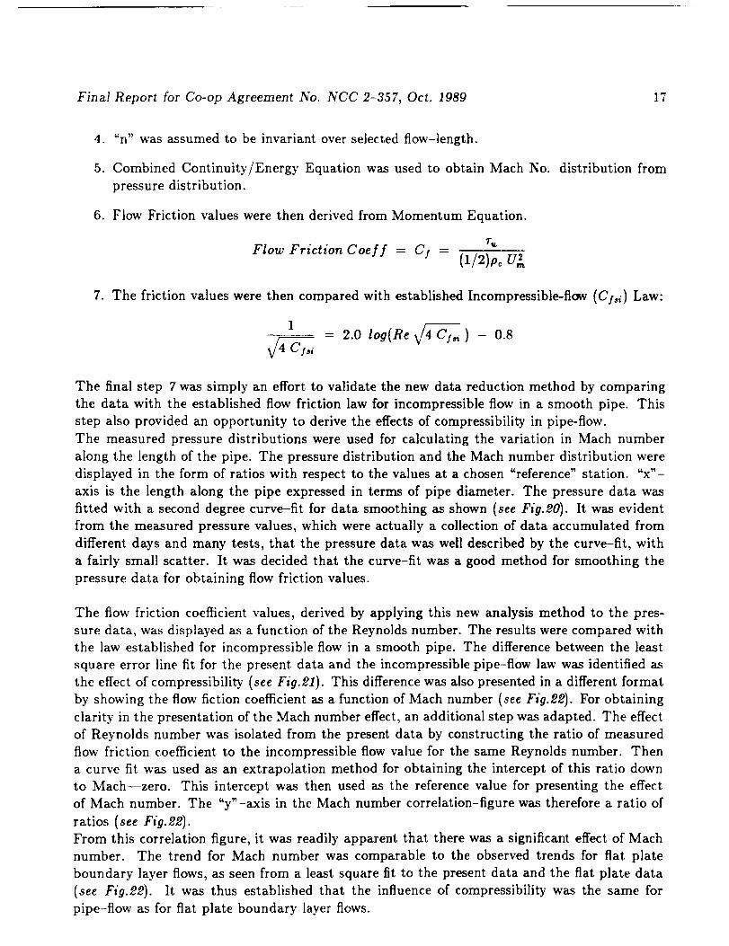
7. The friction values were then compared with established Incompressible-fl(y,v (Ci,i) Law:

2.0 log(Re _44 Cfs i ) -- 0,8

The final step 7 was simply an effort to validate the new data reduction method by comparing

the data with the established flow friction law for incompressible flow in a smooth pipe. This

step also provided an opportunity to derive the effects of compressibility in pipe-flow.

The measured pressure distributions were used for calculating the variation in Mach number

along the length of the pipe. The pressure distribution and the Mach number distribution were

displayed in the form of ratios with respect to the values at a chosen "reference" station. "x"-

axis is the length along the pipe expressed in terms of pipe diameter. The pressure data was

fitted with a second degree curve-fit for data smoothing as shown (see Fig.20). It was evident

from the measured pressure values, which were actually a collection of data accumulated from

different days and many tests, that the pressure data was well described by the curve-fit, with

a fairly small scatter. It was decided that the curve-fit was a good method for smoothing the

pressure data for obtaining flow friction values.

The flow friction coefficient values, derived by applying this new analysis method to the pres-

sure data, was displayed as a function of the Reynolds number. The results were compared with

the law established for incompressible flow in a smooth pipe. The difference between the least

square error line fit for the present data and the incompressible pipe-flow law was identified as

the effect of compressibility (see Fig.21). This difference was also presented in a different format

by showing the flow fiction coefficient as a function of Mach number (see Fig.'22). For obtaining

clarity in the presentation of the Mach number effect, an additional step was adapted. The effect

of Reynolds number was isolated from the present data by constructing the ratio of measured

flow friction coefficient to the incompressible flow value for the same Reynolds number. Then

a curve fit was used as an extrapolation method for obtaining the intercept of this ratio down

to Mach--zero. This intercept was then used as the reference value for presenting the effect

of Mach number. The "y'-axis in the Mach number correlation-figure was therefore a ratio of

ratios (see Fig.22).

From this correlation figure, it was readily apparent that there was a significant effect of Mach

number. The trend for Mach number was comparable to the observed trends for flat plate

boundary layer flows, as seen from a least square fit to the present data and the flat plate data

(see Fig.22). It was thus established that the influence of compressibility was the same for

pipe-flow as for flat plate boundary layer flows.

Final Report for Co-op Agreement No. NCC 2-357, Oct. 1989 18

Having thus established and validated a data reduction method for obtaining correct values

of compressible pipe-flow skin friction, it was then possible to pursue the task of calibrating the

buried wire gages for compressible flow speeds.

4.5 Apparatus for flow-Calibration of Buried Wire Gages

As mentioned earlier, the final step in the buried wire gage calibration procedure was to de-

termine the flow-related constant, namely the Equivalent Length Factor. For this purpose, the

pipe-flow apparatus (a 8" dia pipe, about 56 diameters long), was used (see Fig.18). As men-

tioned earlier, the length/diameter ratio of the pipe was large enough to assure a fully developed

pipe-flow. The flow entering the pipe was passed through a honeycomb and several screens so

that the pipe flow would not develop any swirl component. The instrument plugs with the buried

wire gages were installed in the calibration section. The plug mounting port was specially made

to accommodate the 5 inch radius contoured surfaces of the instrument plug in such a way as to

expose only the sensors to the pipe-flow flowline of 1.5" radius. The mounting had a slot with

knife-edged sides and a properly contoured top face that would flush support the faces of the

instrument plug. The sensor elements would then appear through the slot opening, to be flush

to the wall flow in the calibration section (see Fig.18).

The flow passed from the calibration section to an exit pipe which was more than 10 diameters

long so that the pipe flow pattern in the calibration section would be undisturbed. Flow speeds

in the pipe was varied from low subsonic to high subsonic speeds, by changing the orifice plates

at the exit end of the exit pipe. Flow was induced from a vacuum supply. Static pressure

taps in and near the calibration section were used for measuring the pressure drop along flow

length. This pressure drop was then converted to skin friction values by using the pipe-flow

data reduction method described in the earlier section of this report.

4.6 Flow Calibration of Buried Wire Gages

The gages were operated from an existing constant temperature anemometer system. This

Anemometer system had a special operational feature called the Overheat Reference Value

(ORV) Function, which provided an indication of the gage-sensor resistance in flow. This ORV

capability could be used to a great advantage in the data acquisition process, -- it could replace

the need to undertake a time-consuming step of adjusting the control resistor of the system

while determining the 'cold' resistance of the gage sensor. But, the suppliers of the anemometer

system had not provided a calibration of this ORV feature. With a fully calibrated ORV feature,

the anemometer could remain set on the operating resistance value while the ORV indicated by

the 'NULL DISPLAY' function of the system could be noted for later use in deriving the 'cold'

resistance value of the sensor. The 'cold' resistance value could then be used for obtaining the

flow-related 'recovery' temperature, to be used in the calibration laws of the buried wire gage

technique. As a part of the calibration experiments, all the sixteen channels of the anemometer

system were calibrated for the ORV feature, and validated for measurement of the 'cold' resis-

tance value. This new method of determining the 'cold' resistance was incorporated in the data

reduction package, thus reducing the set-up time needed for taking a data point (see Publication

Nos. 4, 5).

Final Report for Co-opAgreement No. NCC 2-357, Oct. 1989 19

The total Nusselt number measured with the gages in these tests were plotted against the

pipe-flow skin friction values derived from wall pressure measurements. The total Nusselt num-

ber represents the total heat rate delivered from the anemometer system to the sensor, and

contains contribution from flow as well as conduction loss into substrate. The x-axis of this

plot format was shifted for clarity (see Figs.23). The skin friction was shown in the form of a

non-dimensional quantity based on the flow variables associated with it in the calibration law.

The number includes the effects of local density. The results clearly validate the characteristics

of the calibration law. The format of the figure also illustrates the effect of conduction loss on

the sensitivity of measurements. The intercept at no-flow, zero skin friction, is relatively large

even for the present choice of substrate (see Figs.'28). It is therefore very important that the

substrate be well chosen to keep the conduction loss to a minimum.

4.7 Buried Wire Gage Calibration Checks

Some of the gages were used for making extensive calibration checks, by operating those in

the pipe-flow flowfield for a wide range of flow speeds. The calibration constants derived from

earlier measurements in the pipe-flow were used for obtaining the flow-friction values. These

measurements were compared with the actual flow-friction values determined form wall-pressure

measurements. The comparison was very good, as could be seen from the tight cluster of data

points on the line of perfect agreement (see Figs.2_).

4.8 Calibration Constants of Typical Buried Wire Gages

Calibration constants, namely the Conduction Loss Factor A, and the Equivalent Length Factor

B, of the entire 120 gages were reviewed in an effort to identify any opportunities for reductions

in the calibration effort. The idea was to determine if, for gages which were identical in size,

the calibration constants could be considered equal. As it happened, this was not the case. The

differences in the calibration constant values were significant (8cc Figs.'25).

In an attempt to further explore the opportunities for reductions in calibration effort, the gage

calibration constants were placed on a cross-correlation plot (see Figs.'26). The figure displayed

the correlation plot for all the gages that were calibrated in the present effort. It was again clearly

evident that the correlation was not tight enough to justify a carry-over procedure for calibration

constants. The obvious conclusion was that each gage must be calibrated individually.

Final Report for Co-op Agreement No. NCC 2-357, Oct. 1989 2O

5 Instrumentation- Hot Wire Probes, Transducers_ etc.

5.1 Hot Wire Probes

Hot wire probes were fabricated to allow measurements of freestream turbulence. Traversing

screw-slides were mounted on a few Instrument Plugs so that a hot wire probe could be positioned

at any desired distance from the wall layer of the flow.

5.2 Pressure Transducers

Pressure transducers were installed in a few of the Instrument Plugs to facilitate measurement

of the fluctuating pressure level at the wall flow region (see Figs.27).

5.3 Data System

SWTS (Standard Wind Tunnel System_, the data system of the NASA-Ames Unitary Wind

Tunnel facilities, was the main source of acquiring and archiving the test data. A PC-clone was

used for interfacing the anemometer system with the S WTS system.

Computer--controlled scanivalves were used in the initial series of preliminary tests to acquire

wall static pressure distribution along the BLASTANE Test Section. After some attempts to

overcome some of the operational and maintenance problems of the scani-valve system, it was

decided to use an alternate pressure measurement system, namely the 'PSI' (Pressure Systems

Inc.(_) electronically scanning pressure measurement system. Data from this system was also

readily processed through the S WTS system.

Final Report for Co-op Agreement No. NCC 2-357, Oct. 1989 21

6 Experiments

6.1 Preparation for Experiments

BLASTANE Apparatus

It may be noted for quick reference here that the BLASTANE (Boundary Layer Apparatus

for Subsonic and Transonic flow Affected by Noise Environment) apparatus was made fully

operational during the early stages of the term of the present Co-operative Agreement (see

Publication No. 3). However, as mentioned earlier, it had become clear that the acoustic noise

level in the room was rather excessive, large enough to cause a high pressure fluctuation level,

in excess of 95 dBA, in the entry flow of the apparatus. It was known that this level of noise

would adversely affect the capability to generate a complete set of baseline data on boundary

layer flow for very low noise levels-- a limitation which could not be accepted in the scope of

the present Cooperative Agreement. Steps were therefore taken to reduce the noise level. The

pipes and the bellows in the BLASTANE piping were wrapped with noise suppression material,

and the noise level at the entry end of the Air Intake Chamber was reduced to less-than 85 dBA.

Buried Wire Gage Calibration Experiments

Activities relating to experiments included the setting up of the pipe-flow apparatus for a series

of tests pertaining to calibration of the large number of buried wire gages. These tests have

already been discussed in an earlier section of this report (see section _).

Flow Characterization Experiments

The next stage in the experimental program was to to extend the entry-flow length of the BLAS-

TANE flow circuit (see Publication No. 7_, so as to undertake tests relating to characterization

of flow quality emerging from commonly used flow conditioning devices. Additional parts were

designed for BLASTANE. These were to be capable of a_commodating ring-inserts fitted with

different samples of commonly used flow conditioning elements, such as screens of different mesh

sizes and open-area ratios, honeycombs of different cell sizes, heat exchanger panels, etc. With

these types of inserts, it was possible to introduce the different flow conditioning elements at

any desired relative location in the BLASTANE flow circuit.

With respect to the type of entry flow conditions for which the flow conditioning elements

must be tested, it was known that the overall flow pattern and the turbulence levels at entry

to any typical turbulence reduction device in large wind tunnels would be highly non-uniform

across the cross section. Based on data from many tunnels, in particular from the flow measure-

ments in the NASA-Ames 12 FT PWT, it was expected that the flow velocity profile emerging

from the wide angle diffuser, ahead of the turbulence reduction devices, would be typical to a

separated-flow profile, with very low velocities near one wall and high velocities near the other

wall (see Fig.28). This flowfield would also exhibit large flow angles at entry to the Turbulence

Reduction System (TRS) system. One other notable feature of such typical flowfield, as evi-

denced by the 12 FT PWT flow measurements, was that the turbulence levels and scale lengths

Final Report for Co-op Agreement No. NCC 2-357, Oct. 1989 22

would be very large, obviously because those would have been inherited from the large dimen-

sions of the flow passage, and the large size of turning vanes. It thus became clear that the

entry flow conditions for the flow characterization tests should refect large velocity gradients,

high turbulence levels, and large length scales.

With respect to the different flow conditioning element types that need to be studied

for the flow characterization tests, it was clear that screens and honeycombs must be included.

The role of a heat exchanger was not clear. However, recent research had shown that typical

heat exchangers could also be regarded as a part of the TRS. The present author reviewed ex-

isting literature on the flowfield emerging from a heat exchanger, and determined that the heat

exchanger could be treated, and designed-in, as a part of the TRS. The author's review showed

that the exit flow from a parallel plate type heat exchanger would be similar to the exit flow

from a honeycomb, the characteristic length being the tube-spacing.

With the above reasoning, it was decided that the studies for characterization of the flowfield

in large wind tunnels should include some studies of heat exchangers as a turbulence reductionelement.

Prior to conducting tests on the flow characterization aspects, an attempt was made to ex-

amine the possibilities of computing the properties of the flowfield emerging from typical flow

conditioning devices. However, given the complexity of a typical flowfield entering the TRS and

the limitations of the existing literature (and database] on large-level flow variations, it was not

possible to construct a reliable prediction method for calculating the properties of the flowfield

at the exit from the TRS. More detailed data on TRS elements, with larger variations in entry

flow properties, was needed in order to establish a reliable flowfield prediction method. It was

therefore decided that the tests should be conducted rightaway.

The additional parts needed to extend the entry length of BLASTANE, and the ring inserts

equipped with different types of flow conditioning elements were fabricated and assembled in

the BLASTANE flow circuit. It is relevant to note here that the flow characterization tests were

combined with another test program which was aimed at providing a database on turbulence

reduction elements to be used in the NASA Ames 12 FT PWT restoration project. The addi-

tional parts brought the BLASTANE to the configuration described below:

Final Re_ort for Co-op Agreement No. NCC 2-357, Oct. 1989 23

Mortified BLASTANE Apparatus - Brief Description (see Fi9.29)

ITEM DESCRIPTION I

Overall Type • vacuum driven wind tunnel, choked (sonic) exit flow from test section.

• long test section, smooth walls (low wall-induced disturbances)

Flow Speeds • Test Section Mach= 0.19 to 1.0, atmospheric stagnation.

Test Section • 10 inch dia., 72 inch long, very smooth wall surface.

Contraction • 20:1

Low-speed region • long flow length with Flow Chambers, Probe Chambers.

Flow Chamber

Probe Chamber

i •

6 chambers, 54 inch dia, 24 inch long, interchangeable location.

may be fitted with screen rings, honeycombs, frame-work,

heat exchanger panels, wide angle diffuser models.

• 3 chambers, 45 inch dia, 24 inch long.

• may be located between any two Flow Chambers.

• has a traversing Probe-Strut with a Probe-head at the tip.

• Pitot probes, 3-element and 1-element Hot Wire Probes,

and other probes may be mounted in the Probe-head.

Entry Chamber • interfaces Flow/Probe Chambers with Air Intake Chamber.

Air Intake Chr. • fitted with filters to remove any contamination in entry air flow.

Instrumentation

Data System

• SETRA pressure transducers (0.5" H:O), for Pitot probe meas.

• PSI Inc pressure scanners (10" H:O) for pressures in Chambers.

• PSI Inc pressure scanners (5 psid) for pressures in Test Section.• 3-element and 1-element Hot Wire Probes.

• TSI Constant Temperature Anemometer System, 16-channel

• B&K Microphone probes.

• IBM-PC-AT with TSI software for hot wire data acquisition.

• Unitary Wind Tunnel SWTS system.

• REP- VAX for final analysis/compilation of data.

• MAC-H for compilation and preparation of Data Reports.

The simulation concepts adapted for studying the flowfield characteristics of typica] turbulence

reduction system (TRS) of large wind tunnels are explained below:

Final Report for Co-op Agreement No. NCC 2-357, Oct. 1989 24

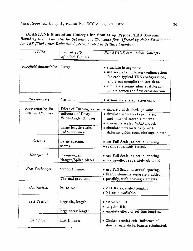
BLASTANE Simulation Concept for simulating Typical TRS Systems

Boundary Layer Apparatus for Subsonic and Transonic flow Affected by Noise Environment

for TRS (Turbulence Reduction System) located in Settling Chamber

ITEM BLASTANE Simulation ConceptsTypical TRS

of Wind Tunnels

Flowfield dimensioins Large • simulate in segments.

• use several simulation configurations

for each typical TRS configuration,

and cross-compile the test data.

• simulate stream-tubes at different

points across the flow cross-section.

Pressure level , Variable. • Atmospheric stagnation only:

Flow entering the

Settling Chamber

Screens

Effect of Turning Vanes

Influence of Entry-

Wide--Angle-Diffuser.

Honeycomb

Heat Exchanger

Contraction

Test Section

Large length-scales

of turbulence.

Large spacing. •

seanls. •

Frame-work. •

Hanger/Splice plates •

Support frame. •

Thermal gradient.

9:1 to 25:1

large dia, length.

large decay length

i Exit Diffuser.

L

Exit Flow

simulate with blockage vanes.

• simulate with blockage plates,

and patched screen elements.

• also use a scaled WAD model.

simulate parametrically with

different grids/rods/blockage-plates.

use Full Scale, at actual spacing.

seams separately tested.

use Full Scale, at actual spacing.

Frame-effect separately obtained.

use Full Scale, at actual spacing.

Frame elements separately added.

possibly, with heating elements.

• 20:1 Ratio, scaled lengths

• 9:1 ratio available.

• diameter= 10"

• length= 6 ft.

simulate effect of settling lengths.

Choked (sonic) exit, influence of

downstream disturbances eliminated.

Final Report for Co-op Agreement No. NCC 2-357, Oct. 1989 25

These simulation concepts helped in arriving at a limited number of BLASTANE configura-

tions, with differently located flow conditioning elements (screens, honeycombs, heat ezchanger

panels), that needed to be tested for characterizing the fiowfield. The Probe Chambers equipped

with flow measuring instrumentation could be located at any desired flow station so as to mea-

sure the turbulence distribution and velocity profile at entry and exit stations of the TRS.

The instrumentation and data system developed for detailed measurements of the flow field

included 3-element hot wire probes, acoustic probes, low-pressure range transducers, flow angle

measuring vanes, and traversing devices (see Figs.80, 31).

Boundary Layer Experiments

The configuration of BLASTANE during the flow characterization tests was also suitable for

some test section wall boundary layer measurements. The buried wire gage signals were analyzed

in order to obtain an appreciation of the boundary layer flowfield. However, at the time of writing

this report, BLASTANE apparatus was still being used for tests pertaining to simulation of the

12 FT PWT Restoration Project TRS design, and was not available for detailed boundary layer

tests.

6.2 Measurements, Results and Discussion

It may be noted here that the calibration tests and measurements for the large number

of buried wire gages were an important part of the experiments, and took up a considerable

portion of the term of the present project. These measurements have been discussed in an earlier

section of this report, and will not be repeated here.

The next phase in the measurements was the one relating to characterization of the turbulence

field in large wind tunnels. As mentioned earlier in this report, the test program pertaining to

the present project was merged with the simulation tests aimed at providing a database on the

design of the Turbulence Reduction System (TRS) of the 12 FT PWT Restoration project. The

test results pertaining to the present project are presented below:

Results from flow-characterization tests:

• Test Section turbulence levels were in the range of 0.03_ to 0.06% for contraction-entry

turbulence levels of up to about 1.0%. For higher entry turbulence levels, the test section

turbulence levels were higher. (see Fig.82)

(Note that the contraction ratio is 20:1)

• Turbulence level in the test section remained invariant from entry to the 36" station (which

was the last measurement station) along the length of the test section.

• Turbulence reduction ratio, i.e., the ratio of test section turbulence to the contraction entry

turbulence, matched the inverse of contraction ratio only for entry turbulence levels higher

than 0.8%, but did not match for lower entry turbulence levels (see Fig.32)

Final Report for Co-op Agreement No. NCC 2-357, Oct. 1989 26

• For a given turbulence level at entry to contraction, the test section turbulence was higher

for higher Mach numbers, perhaps because of compressibility effects (see Fig.32)

A 3-element hot wire probe, containing 50 micron fiber-film elements, was used in the test

section to measure the different components of turbulence. These measurements did not

compare well with the single element hot wire probes containing 5 micron tungsten wires.

It was suspected that the 3-element probe, because of the larger sensor diameter, would

not give proper measurements for flow speeds larger than Mach 0.3. 3-element probes

with slender sensors were not readily available.

It was possible to confirm that, for lower flow speeds, the test section turbulence field was

essentially isotropic.

Test Section wall pressure fluctuation measurements were made with flush-mounted pres-

sure transducers. For the case of low turbulence at entry to contraction, which represented

the baseline flow condition for boundary layer studies, the pressure fluctuations were in

the range 0.33 to 0.5% along the length of the test section.

It may be noted that the exit flow from the test section is choked by a flow control plug in

BLASTANE, entirely eliminating any influence of flow noise downstream of the diffuser.

Higher acoustic noise levels are to be achieved in BLASTANE by introducing an electrically

driven speaker at the entry to the Contraction or Settling Chamber.

Results from Baseline boundary layer measurements:

It was confirmed that the desired baseline Test Section flow condition of very low flow

unsteadiness level was achievable with 5 screens at the entry to the Contraction. Measure-

ments for that configuration showed that the baseline turbulence was in the range 0.03

to 0.08 _, and pressure fluctuations were in the range 0.07 to 0.15 _, depending on the

Mach number (higher levels for higher Maeh nos.).

For the case of baseline flow condition, i.e., low turbulence low acoustic noise level in the

freestream, signals from buried wire gages mounted at several wall stations were analyzed

with the respective calibration data. The gages appeared to perform satisfactorily.

Final Report for Co-op Agreement No. NCC 2-357, Oct. 1989 27

7 Concluding Remarks

The progress made with respect to the objectives of the Cooperative Agreement are summarizedbelow:

Existing research publications were reviewed extensively, to finally determine that the

many theoretical methods that exist for predicting the effects of flow unsteadiness compo-

nents on boundary layer transition may be adequate for low subsonic flow speeds, but are

not reliable for high subsonic flow speeds, primarily because of the effects of compressibil-

ity.

The existing database on boundary layer transition at high flow speeds was reviewed in an

effort to properly isolate the individual effects of Mach number, acoustic pressure fluctua-

tions, and freestream turbulence. A systematic procedure, inspired by the well established

correlations for incompressible boundary layers and the findings of flight experiments, was

evolved to carefully separate the effects of the individual flow unsteadiness components.

New correlation laws were established for the individual effects (see Chapter-2)

The Experimental Apparatus, namely the Boundary Layer Apparatus/or Subsonic and

Transonic flow Affected by Noise Environment (BLASTANE), was fully developed to un-

dertake a testing program for collecting detailed data on the effects of the individual

flow' unsteadiness variables. Acoustic noise levels and turbulence levels in this appara-

tus were reduced to very low levels in order to acquire base-line data for very low mass

flux fluctuations and pressure fluctuations (the two most important parameters in the flow

unsteadiness field).

Baseline Test Section flow conditions were found to be of very low turbulence (0.03 to 0.08

_), and very low pressure fluctuations (0.07 to 0.15 _), depending on the Mach number

(higher levels for higher Mach nos.).

Special instrumentation, primarily the buried wire gage technique, was developed for ob-

taining reliable indications of boundary layer transition, and for measuring wall flow skin

friction distribution. A large number of gages, a total of about 120, were built into the

instrument plugs of the BLASTANE test section, so that the gages could be used for ob-

taining wall-flow properties simultaneously at a series of stations along the length of the

boundary layer flowfield. All the gages were calibrated fully in a standard pipe-flow, and

made ready for detailed boundary layer measurements.

As a part of the gage calibration data reduction effort, a new method was developed

for analyzing compressible pipe flow. This analysis made it possible to correctly derive

wall flow friction values from wall pressure distribution measurements for high subsonic

flow, speeds. The new method consisted of applying an integral technique to transform

the basic compressible flow equations into a set of integral governing equations, and then

applying the knowledge of flat plate compressible boundary layers to provide closure to

those governing equations. This method was validated by performing a special series of

tests on pipe flow, with centerline Mach numbers ranging from low subsonic to almost

sonic, and evaluating the detailed wall pressure measurements (see section ._._).

Final Report for Co-op Agreement No. NCC 2-357, Oct. 1989 28

Buried Wire Gages were mounted in the test section and operated to obtain data at

different freestream conditions. The gages appeared to be performing satisfactorily.

It may be noted that the apparatus and instrumentation were brought to a status at which

boundary layer transition data acquisition tests could be commenced, but the apparatus

was to be used on another higher priority project, namely the 12 FT PWT Restora-

tion Turbulence Reduction System Design Project. It was possible to combine the flow-

characterization tests of the present project with the higher priority project, and obtain a

good database. But, the boundary layer transition tests remained at a lower priority all

the way up to the writing of this final report.

It is recommended that a series of data generation tests for boundary layer transition

phenomena be taken up in a future research project, with the instrumentation developed

in the present project, so that a first-of-the-kind database may be made available in that

subject area.

Final Report for Co-op Agreement No. NCC 2-357, Oct. 1989 29

8

o

.

,

.

.

.

.

List of Publications

Murthy, S.V. and Steinle, F.W., "On Boundary Layer Transition in High Subsonic and

Transonic Flow under the Influence of Acoustic Disturbances and Free-stream Turbulence,"

AIAA Paper 85-0082, Reno, NV., Jan. 1985.

Murthy, S.V. and Steinle, F.W., "Effects of Compressibility and Free-stream Turbulence on

Boundary Layer Transition in High Subsonic and Transonic Flows," AIAA Paper 86-0764,

West Palm Beach, Fl., Mar. 1986.

"Documentation pertaining to design and safety aspects of BLASTANE (Boundary Lager

Apparatus for Subsonic and Transonic flow Affected by Noise Environment)-- Safe Operat-

ing Procedure ('SOP', Document No. A-327C-8401-SD4, Oct. 1986), System Safety Hazard

Action Status Reports (Vol.1 on Preliminary Hazard Analysis Items, and Vol.2 on Oper-

ational Hazard Analysis Items, Document Nos. A-327C-8401-SD1 and SD-2, Oct. 1986),

Integrated Systems Test plan ('IST--plan', Document No. A-327C-8401-SD5, Oct. 1986),

Completion of the Integrated Systems Test for BLASTANE ('IST--completion tests, Doc-

ument No. A-327C-8401-SDS, Feb. 19, 1987), Aerodynamic Facilities Branch (Code RAF),

Engineering Documentation Center, NASA Ames Research Center, Moffett Field, CA,

1986-87.

Murthy, S.V. and Steinle, F.W., "Calibration Data for Buried Wire Gages to be used in

BLASTANE Experiments", Calibration Data Report, (Internal Report) prepared under

Co-op Agreement No. NCC 2-357, Aerodynamic Facilities Branch, NASA Ames Research

Center, Oct. 1986.

Murthy, S.V. and Steinle, F.W., "Development and Calibration of Buried Wire Gages

for Wall Shear Stress Measurements in Fluid Flow", accepted for presentation as Paper

No. 88-2022 at the AIAA 15th Aerodynamic Testing Conference, San Diego, CA, May 18-

2O, 1988.

Murthy, S.V., K. Gee, and Steinle, F.W., "Compressibility Effects on Flow Friction in

a Fully Developed Pipe Flow", accepted for presentation as Paper No. 57 at the First

National Fluid Dynamics Congress, Cincinnati, OH, July 25-28, 1988.

"Simulation Studies of Flow Quality Characteristics and Control in a Closed-loop Wind

Tunnel Circuit", -- Documentation pertaining to (i) use of BLASTANE Apparatus for

studies of flow characteristics emerging from commonly used flow conditioning elements,

(ii) Proposed additions to the Apparatus for acquiring test data on flow conditioning ele-

ments, (iii) Aerodynamic loads for Modifications of BLASTANE, etc., by S.V. Murthy and

F.W. Steinle, submitted to Aerodynamics Division -- 12 FT PWT Restoration Project,

NASA Ames Research Center, Moffett Field, CA, Jan--Mar. 1988

t,..) ZZC)

,-4 I.--

i-v- I-.=_ t,.)

I..LJ I,_

Lt. r,

Z

L_INif)Z

0.-J

I,0

ILl

0

Z

I'--0

I--

0.

ILlI--

tz_

J,,ZZ

t--

_-_Z,., _L_ i.t.J

Z t.._,._"iX: ,_"0 =" c_ I-- 0

I.-- Z =" _" _-

I-- _ 0 I._ _

Z O...I,._l_ "_,

I II I

v"!

%

Z

I--

_,,, c_Z _...)r_

_C_

i

4-

L_

m

L:.

EFFECT OF MACH NUMBER ON BOUNDARY LAYER TRANSITIONCONE DATA, FOR LOW FLOW UNSTEADINESS LEVELS

_,-_X-_ FLIGHT DATA ENVELOPE !_ AEDC 16 T[] ARC11TWT V LRC 16TT

ARC 14 TWT D NSR&DC 7x10 TA LRC 8 TPT <] LRC 16 TDT

PRESENT CORRELATION

I I I

I BEGINNING OF TRANSITION!I

I 8 RetI

[ aM= 3×10 6

I I I

i I

FLIGHT DATAENVELOPE

CORRELATION SLOPE = 3 × 106

I I I

I t

-1.5

-2.0

-.4

Figure 4.

END OF TRANSITION

a Re T- 3X10 6

bM

FLIGHT DATAENVELOPE

r_

CORRELATION SLOPE = 3 × 106

I I I-.3 -.2 -.1 0 .1 .2

INCREMENTAL MACH NO. = (M-0.8)

TR_XSITIOX REt.'NOLDS N_BIBER AS A FUNCTION OF MACH N_BER

x®_ ×_

W_=.I ,_ .J Z (J J 0 ([

.... I--_:

=_ _ !

=PPP_U

0 _u_uu==

Z

m Jooo<mb

7 <or.j ,.J

i I i I I |

9_OL x .l.ou

_z

<_

N,=.

t.n

IIIII

1

O 13 (><] ,d b l _ i _

9_OL x be '.L_I:I

ZOu_F_.ZzuJ

i

:::)CIILl

FI

0I--0IllIJ.LLIll

OZ

Z _J

eoIn

oo

OZ

Z_

IIIIII

L

¢6

I I I I

be 'lal:t 'be '_'el:l9_0L x

(B'O : IN Ol O3 EIEI3::I31:::I)EI381/_nN SC]7ONA3EI NOIIISN_I::II

o

[-

iil L_-

Z

L_

L..-,

I,,O

In" _ •

L-,

IT" 1 I I 1

[_ '-!-o1::t/_ %1::i]

=o

I,,0

<

r,,,'

o

" Z]

,p _ z

Z

0

\

>

<z0

I

_L

LLIZ

_c,_.,a

LL

ORIGINAL PAGE IS

OF POOR QUALITY

Figure 1 1. ,,BL_,.S-Iu_3,_":_Pp:'c_-'_7_.JS- TEST SECi-IOX

ORIGINAL PAGE IS

OF POOR QUALITY

SCHEMATIC OF BURIED WIRE GAGE TECHNIQUE

EDGE OF

BOUNDARY LAYER

VELOCITY PROFILE

FLUID FLOWBOUNDARY LAYER

THICKNESS. 6

FLOW SURFACE

\

\

/ALUMINUM INSTRUMENT

PLUG BLANK

CABLE LEADING TO

ANEMOMETER SYSTEM

BURIED ' HOT '

WIRE SENSOR

SUBSTRATE INSERT

Figure 15. SCHEMATIC OF BURIED WIRE GAGE TECHNIQUE

ID

w_• :EZ

oo_ .., _ "' L_'_%4oZ --

=)<{: _z _z_ !_\\_LL (_ UJ,,-- ,_ IK \ \\ _ '" \

r,l i_1 ,=, a:_ ,',, u

I11

Zin_. , ,.. _,...-,.I_--_ ,_ _- I

___-_ . < z

Zr,/)_ m ,,,":: z_o___ 0 _,0 L_-' l-- u,. J uJ __

:_ Z ._< zz_<_z ,.i.Id f._ v, ..i. .._

_0 "_. < 3 _x ,_- w -<I,i,I I_ W ". .i =', >-_Ow li.l E_ _ =_.._=Z ILl

•_, _ x _>_ "=__u_ _ _l'_:Z u_

_.3o /

_ '_ ,,7,'/,7//I.;Z(/,

_o 17- ,_ _l "-_

I

,I

1:1:

!!z

5-

c_

¢/%

IaJ

C_gCC

i.¢J

C_

Ca

L:-

INSTRUMENT PLUG BLANK WITH BURIED WIRE GAGES

INSTRUMENTPLUG BLANK

CABLE LEADS

PLUG BLANK WITH 5 GAGES

POLYSTYRENESUBSTRATEINSERT FLUS_MOUNTEDON THECONTOUREDPLUGSURFACE

POLY-STYRENESUBSTRATE

'HOT' WIRE SENSOR

(3.8 _m diamTUNGSTEN) WELDEDTO ELECTRICAL LEADSAND SOLVENT-BONDED

TO THE SUBSTRATESURFACE

ELECTRICAL LEADS

(0.38 mm diam NICKEL)

MAGNIFIED VIEW OF A BURIED WIRE GAGE

Fi_/re 15. INSTRUMENT PLUG BLAhU< WITH BURIED WIRE GAGES.

ORIGINAL PAGE IS

OF POOR QUALITY

SQUARE-WAVE

TEST SIGNAL

GENERATOR

FLOW

ANL'MOM'ETER BRIDGE AND TEST SIGNAL CIRCUIT

R5

R

GAGE SENSOR

R 3

AMPLIFIED OFF-BAlANCE

(OVERHEAT REFERENCE)

FEEDBACK

A.MPLIFIER

OSCILLO-

SCOPE

(a) ANEMOMETER BRIDGE CIRCUIT AND FEEDBACK SYSTEM

UNFILTERED

SIGNAL

FILTERED

SIGNAL

_---20 micro-sec

(b) OSCILLOSCOPE TRACE OF SQUARE WAVE TEST SIGNAL RESPONSE

Figure 16. _NEMOMETER BRIDGE AND TEST SIGNAL CIRCUIT

ORIGINAL PAGE |8

OF POOR QUALITY

t-,-

C)

I-,

.,--_

ORIGTNAL PAGE ISOF POOR QUALITY

ORIGINAL PAGE IS

OF POOR QUALITY

l'51

z0I"-

I'-"¢,/)

Z0D

I-,

I-"c_

,+ ÷

_=,.,

"-' >.

! 1 I I

c_

0z

<

_J

z

r_

uJ

zL_

C_C_0

R

0

UP

0

dz

<

uJF.-

z

(J

0

Cr)

rr

II

EE

|

k_

U

n-O

<<<<<<<_

0000000

_ _-

i

0

( I I.

A

EE

X

Z<

a

MACH NO.

[] 0.674 _ 0.302

0 0.568 V 0.228

L_ 0.388

-- _ -- LEAST SQUARES LINE FIT

THEORETICAL CURVE, SMOOTH PIPE

O,.,JIt.

.006 i l

¢._ .005 k / LEAST SQUARE ERROR 1

/

_ .003 1 •= 2.0 Io9 (Re_,/-4"_f=i) - 0.8

.002 I I

105 2 x 105 5 x 105 106

REYNOLDS NUMBER. Re

MURTHY

Figure 21, PIPE-FLOW FRICTION COEFFICILNT AS A FUNCTION OF REYNOLDS NL_ER

Figure 22.

1.1

1.0

o .9

A.w

C9

.8

,6

.50

EFFECT

[]0

COMPARISON STANDARD:

APPX Re NO.

690000 O 390000

620O00 _7 30O000485000

LEAST SQUARES CURVE FIT. (Cf/CIti)M. 0 = 1.0396

1= 2.0 log (Re v/'4"_s , ) - 0.8

! I I 1

THEORY, FOR /

FLAT PLATETURBULENTBOUNDARY LAYER.

(REF. 2)LEAST SQUARE ERRORCURVE FIT FOR THEEFFECT OF MACH NUMBER.

(PRESENT PIPE-FLOW DATA)

OF

I I 1 I

.2 .4 .6 .8

MACH NUMBER

.0

MURTH¥

C06IPRESSIBILITY ON PIPE-FLOW FRICTION COEFFICIE.XT"

uJl',, ml' 0 _ _'=

00_ 0 b

E=.

.m

I-Ou.

Z'r

,,,ai

_Z

qJ.=_

I-Z

I-

Z0U

-- Z

'" w

,1,

Z1,- w-- Z

o

!

I00<_ + x

\7,.

\

\

\\\\\

i I 1 1 I i I I i i i I I I ! I I

i 00 ,r-

SIN3_3_IFISV31_ 3OYO .'M'BIAIOi:I::I'm_,e'MI

\L_

I

o

00I--Zl,IJ

_El.u

r_

iJJ

U..l

_o

LP

0

c_

C'-,.I

c_I.-

• ,,,-i

Oee _-0 0

0 u.

t_ Z

-J .J

Z _-0 Z

WI- _j

>Z0 0t_ w

O0

.E

---I0

V '8010V3

S_O"I "GNO0

3

3

"3

".z_-

z

m

I.U

I,LI

:B "OV.-I

HION=I'! "AIN03

8,:7 ¸0

CORRELATION FOR CALIBRATION CONSTANTS OF B.W.GAGES

EQUIVALENT LENGTH FACTOR VERSUS CONDUCTION LOSS FACTOR

D Gages with 4.0 micron dia, 1.2mm Ion I sensorsLeast squares line fit

9.0

0

0

>°,=._

8.0

7.0

6.0

5.0

4.0

3.0

o B _

0

n

I0

D0

[3[3

[3

O

I ] 1 1 I I

1.5 1.6 1.7 1.8 1.9 2.0

Conduction Loss Factor, A

2.1

Figure 20. CORRELATION FOR CALIBRATION CONSTANTS OF BURIED WIRE GAGES

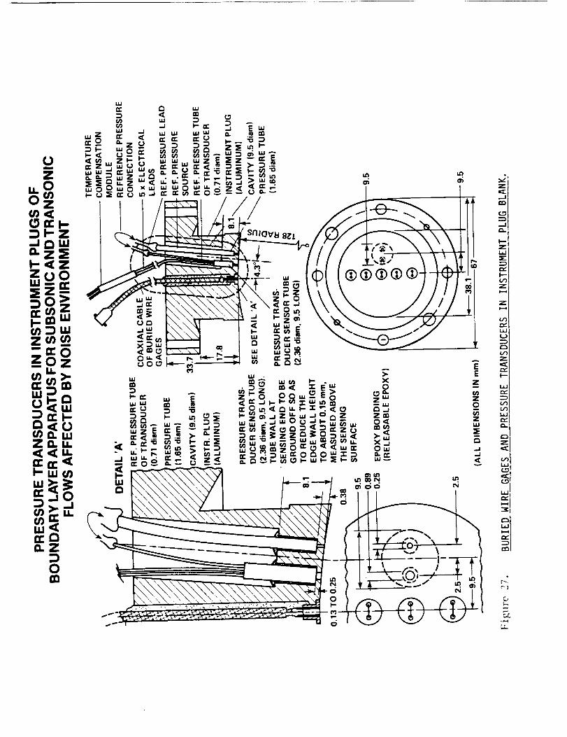
| t

!!

U.

[ii,

[..U9Z

LD

[-

(Q

°,..Ii

Z.<

m

111

iU

\

I

[]

m

I I

I

fuiu_l

II

-I_.iI

k

..2:..3

0

-,, ,..,

(uofle/s-.9C o/ ,{J/ua LUOJ/)

% 'll/,n "UOl|OeS lsel Ul leAel eOuelnqJnj.

q)

L--

t-G)

¢-

i

¢)¢D

0

=E,