Pedestrian Control Issues at Busy Intersections and Monitoring Large Crowds

2002-29 FinalReport

PEDESTRIAN CONTROL ISSUES AT BUSY INTERSECTIONS AND

MONITORING LARGE CROWDS

Prepared by:

Benjamin Maurin, Osama Masoud, Scott Rogers, Nikolaos P. Papanikolopoulos

Artificial Intelligence, Robotics, and Vision Laboratory

Department of Computer Science and Engineering

University of Minnesota

Minneapolis, MN 55455

March 2002

Published by:

Minnesota Department of Transportation

Office of Research Services

First Floor

395 John Ireland Boulevard, MS 330

St. Paul, MN 55155

The contents of this report reflect the views of the authors who are responsible for the facts and accuracy of the data presented herein. The contents do

not necessarily reflect the views or policies of the Minnesota Department of Transportation at the time of publication. This report does not constitute a

standard, specification, or regulation.

The authors and the Minnesota Department of Transportation do not endorse products or manufacturers. Trade or manufacturers’ names appear herein

solely because they are considered essential to this report.

Technical Report Documentation Page1. Report No. 2. 3. Recipients Accession No.

MN/RC – 2002-29 4. Title and Subtitle 5. Report Date

March 2002 6.

PEDESTRIAN CONTROL ISSUES AT BUSY INTERSECTIONS AND MONITORING LARGE CROWDS

7. Author(s) 8. Performing Organization Report No.

B. Maurin, O. Masoud, S. Rogers and N. Papanikolopoulos 9. Performing Organization Name and Address 10. Project/Task/Work Unit No.

11. Contract (C) or Grant (G) No.

University of Minnesota Artificial Intelligence, Robotics and Vision Laboratory Department of Computer Science and Engineering 200 Union Street, S.E. Minneapolis, MN 55455

c) 74708 wo) 122

12. Sponsoring Organization Name and Address 13. Type of Report and Period Covered

Final Report 2000-2002

14. Sponsoring Agency Code

Minnesota Department of Transportation Office of Research Services 395 John Ireland Boulevard Mail Stop 330 St. Paul, Minnesota 55155

15. Supplementary Notes

16. Abstract (Limit: 200 words)

The authors present a vision-based method for monitoring crowded urban scenes involving vehicles, individual pedestrians, and crowds. Based on optical flow, the proposed method detects, tracks, and monitors moving objects. Many problems confront researchers who attempt to track moving objects, especially in an outdoor environment: background detection, visual noise from weather, objects that move in different directions, and conditions that change from day to evening. Several systems of visual detection have been proposed previously. This system captures speed and direction as well as position, velocity, acceleration or deceleration, bounding box, and shape features. It measures movement of pixels within a scene and uses mathematical calculations to identify groups of points with similar movement characteristics. It is not limited by assumptions about the shape or size of objects, but identifies objects based on similarity of pixel motion. Algorithms are used to determine direction of crowd movement, crowd density, and mostly used areas. The speed of the software in calculating these variables depends on the quality of detection set in the first stage. Illustrations include video stills with measurement areas marked on day, evening, and indoor video sequences. The authors foresee that this system could be used for intersection control, collection of traffic data, and crowd control.

17. Document Analysis/Descriptors 18.Availability Statement

Tracking Pedestrian control

Detection Crowds

No restrictions. Document available from: National Technical Information Services, Springfield, Virginia 22161

19. Security Class (this report) 20. Security Class (this page) 21. No. of Pages 22. Price

Unclassified Unclassified 48

Executive Summary

This project provides a new way of looking at pedestrian control issues at busy intersections.

Furthermore, we can use the proposed techniques to monitor large crowds. We used our experience

in handling scenes with a small number of pedestrians to handle cluttered scenes at busy

intersections. Instead of focusing on the detection or tracking of single pedestrians, we focused on the

detection and tracking of crowds. Our approach employs an effective detection scheme based on

optical flow that can locate vehicles, individual pedestrians, and crowds. The detection phase is

followed by the tracking phase that tracks all the detected entities. Traffic objects are not simply

tracked but a wealth of information is gathered about them (position, velocity,

acceleration/deceleration, bounding box, and shape features). Potential applications of our methods

include intersection control, traffic data collection, and even crowd control after athletic events. We

illustrated our approach to busy (with respect to the number of pedestrians) intersections and the

development was on a PC-based system with a C80 board. Finally, we illustrate our approach in

video sequences of large crowds (athletic events, schools, underground scenes, etc.).

TABLE OF CONTENTS

Chapter 1 Introduction ...............................................................................................................1

Previous work.....................................................................................................................................2

Chapter 2 Image Processing.......................................................................................................5

Detection ............................................................................................................................................5 Nature of the Video Sequences and Preprocessing ........................................................................6 Background Removal .....................................................................................................................6 Motion Extraction...........................................................................................................................7

Optical flow........................................................................................................................................8 Definition........................................................................................................................................8 Mathematical Approach .................................................................................................................8 Differential Method........................................................................................................................9 Correlation Method ........................................................................................................................9

Background ......................................................................................................................................14 Segmentation....................................................................................................................................14

Clustering the Motion Map from the Optical flow.......................................................................15 Two Features Computed by the Segmentation.............................................................................17

Chapter 3 Tracking ..................................................................................................................19

Layer model......................................................................................................................................20 First Level: Blobs .........................................................................................................................20 Second Level: Regions.................................................................................................................21

Geometrical description of the entities.............................................................................................21 Oriented Boxes .............................................................................................................................22

Details of relations ...........................................................................................................................24 Relations Based on Scores ...........................................................................................................24 Heuristic Combination .................................................................................................................25

State space representation of regions ...............................................................................................26 State Vector and Data Splitting ....................................................................................................26 Position Characteristics ................................................................................................................28 Shape Features..............................................................................................................................28

Kalman filtering ...............................................................................................................................29 Position Filtering ..........................................................................................................................29 Shape Filtering .............................................................................................................................30 Parameter Values..........................................................................................................................30 Initialization..................................................................................................................................32

Chapter 4 Results and Conclusions..........................................................................................33

General comments............................................................................................................................33 Statistics ...........................................................................................................................................34 Mostly used area...............................................................................................................................35 Tracking results ................................................................................................................................36 Conclusions ......................................................................................................................................36

References .................................................................................................................................41

LIST OF FIGURES

Figure 1. Traffic Scenes from the Xcel Energy Center in St Paul. ........................................................5 Figure 2. Background creation. ..............................................................................................................7 Figure 3. Two detection zones going in opposite directions..................................................................7 Figure 4. Optical flow and motion flow. ................................................................................................8 Figure 5. Correlation approach.............................................................................................................10 Figure 6. Two ways to see the correlation............................................................................................11 Figure 7. Classic methods for segmentation. .......................................................................................15 Figure 8. Tracking system. ...................................................................................................................19 Figure 9. Oriented box on a distribution. .............................................................................................23 Figure 10. Overlap Area.......................................................................................................................24 Figure 11. Mostly used areas during two minutes of day video. .........................................................36 Figure 12. Results from a day video. ...................................................................................................37 Figure 13. Results from a night video. .................................................................................................38 Figure 14. Results from a real-time video............................................................................................39 Figure 15. Results from a winter video. ...............................................................................................40

LIST OF TABLES

Table 1. Comparison of classical algorithms for segmenting an image.............................................. 16 Table 2. Statistics on 821 frames during 120 seconds ........................................................................ 35

1

CHAPTER 1

INTRODUCTION

Monitoring crowded urban scenes is a difficult problem. Despite significant advances in traffic

sensors, modern monitoring systems cannot handle effectively busy intersections. The reason is that

there are too many moving objects (vehicles and pedestrians). Tracking humans in outdoor scenes is

also very complex. The number of pedestrians and vehicles in a scene varies and is usually

unpredictable. Recently, there was progress on techniques to track an arbitrary number of pedestrians

simultaneously. However, as the number of pedestrians increases, system performance degrades due

to the limited processing power. When the number of pedestrians exceeds a threshold value, the

processing rate drops dramatically. This makes it hard to keep accurate track of every pedestrian and

vehicle because of the large displacement among pedestrian and vehicle locations in the processed

frames.

We propose a vision-based system that can detect, track, and monitor busy urban scenes. Our

system is not only limited to vehicles but can deal with pedestrians and crowds. Our approach is

robust to a variety of weather conditions and is based on an efficient scheme to compute the optical

flow. The optical flow helps us classify the different objects in the scene while certain statistics for

each object are continuously updated as more images become available.

Addressing busy intersections can have a significant impact on several traffic operations in urban

areas and on some more general applications. One traffic operation which can be affected is the

automated walk signal request. Currently, a pedestrian is required to press a button to request a walk

2

signal at a crosswalk. It may be desirable to automate this process especially when there is a large

number of pedestrians waiting to cross the street. Crowd detection can be used in this case. Another

application is the study of flow patterns at certain intersections. It may be desirable as a city planning

consideration to study the use of crosswalks at a certain intersection. Flow data of pedestrians

crossing the street throughout the day can be collected and used to make decisions such as building a

pedestrian bridge, etc. Finally, our proposed system may be used to monitor crowds outside schools,

nursing homes, train tracks, and at athletic events. One interesting application is to compute crowd

density (with obvious public safety applications). In general, monitoring areas where accidents occur

often can result into early warning signals and can reduce deadly consequences.

The paper starts with a review of previous work, continues with the detection and tracking

schemes and concludes with experimental results.

PREVIOUS WORK

Many methods have been proposed for the detection and tracking of moving objects; many of those

have focused on the detection and tracking of traffic objects. The applications of this line of research

are multiple: tracking of targets, vision-based robot manipulators, presence detectors, analyzers of

visual data, etc.

The first generation trackers made several assumptions regarding the nature of the objects in the

scene. These assumptions resulted in acceptable tracking performance but on the other hand, they

were not robust to changes in the scene (e.g., movement of the camera or small changes in the shape

of the object). Baumberg and Hogg [1] introduced one of first trackers. It was based on active

3

contours to track the silhouette of a person. Others, such as Rossi and Bozzoli [2], addressed the

problem by locating the camera above the scene, which avoids the creation of occlusions. But this

kind of practice is not easy to implement especially in traffic applications. The systems described

require extensive models of the objects to be tracked. They also require some knowledge of their

dynamic characteristics. We are going to use only a few assumptions on the models in order not to

restrict our tracker to a single class of detection. For example, no limits will be assumed for the

velocities of the traffic objects, their sizes, their acceleration, or their shape.

Systems based only on a background subtraction give good results but fail to detect and track

traffic entities when they get close to each other. One example of such a method can be found in [3].

Our system extends that approach by utilizing motion cues.

Cutler and Tuck [4] developed a recognition and classification module for motion. It aimed to

interpret gestures. Their work is based on the analysis of moving areas in a video sequence. This

makes it more of a motion classifier than a tracker. Our detection method is close to [4] and to

Dockstader’s work [5], which addressed robust motion estimation.

4

5

CHAPTER 2

IMAGE PROCESSING

DETECTION

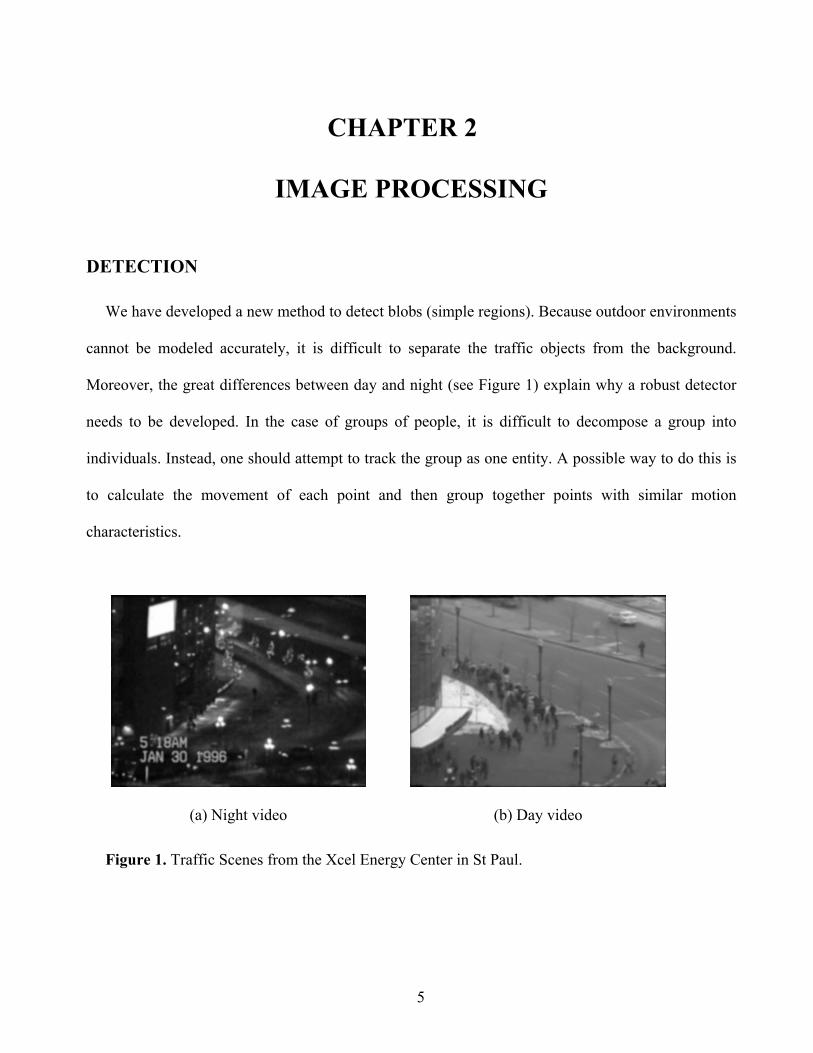
We have developed a new method to detect blobs (simple regions). Because outdoor environments

cannot be modeled accurately, it is difficult to separate the traffic objects from the background.

Moreover, the great differences between day and night (see Figure 1) explain why a robust detector

needs to be developed. In the case of groups of people, it is difficult to decompose a group into

individuals. Instead, one should attempt to track the group as one entity. A possible way to do this is

to calculate the movement of each point and then group together points with similar motion

characteristics.

(a) Night video (b) Day video

Figure 1. Traffic Scenes from the Xcel Energy Center in St Paul.

6

Nature of the Video Sequences and Preprocessing

Images from the outdoor video sequences that we used are grayscale. We do not make any

assumptions on the nature of the scene (e.g., night, day, cloudy, rainy, winter, summer, etc.).

Elements of the scene are not known a priori and the sizes of the traffic objects (vehicles and

pedestrians) are also unknown. An assumption that we make is that a crowd is a slow deformable

object with a principal direction of motion.

This assumption is not restrictive for our objectives, but it can be restrictive in the case of

vehicles. A traffic tracker must be able to track objects that vary from a simple pedestrian to a

complex crowd.

Outdoor images can have very bad quality, especially at night. In the preprocessing phase, it is

necessary to remove noise. We achieve this goal by convolving the images with a Gaussian filter. We

can also apply a mask to the image to remove the undesired regions such as roads, flashing

billboards, or reflective building walls.

Background Removal

Haritaoglu et al. [6] modeled the background by following a statistical approach. The detection of

people is achieved by subtracting this background from the new images (see Figure 2). The

parameters of the background are re-evaluated with every new image. The model uses a Gaussian

distribution for each pixel and a comparison-evaluation for every frame. The classification of

foreground/background is done at this time by combining all the previous results. This approach

creates a very good separation between the two possible classes (foreground, background). However,

no other information can be extracted from this technique. In particular, during the motion of two

crowds past each other, one cannot estimate the speed or direction. This method is useful in the case

7

of easily distinguishable objects with slow motion. In our case, a pixel-by-pixel scan would be

relatively slow.

(a) First image (b) Background model (c) Detected blobs

Figure 2. Background creation.

Motion Extraction

Another idea for the detection part of our approach is to consider the optical flow for a precise

extraction of the motion in the scene. It is a very difficult problem to solve in real-time, however.

This paper tries to address some of the computational issues related to optical flow estimation. Like

Sun [7], Dockstader et al. [5], and other researchers, we will concentrate on the speed requirements

of the algorithm, more than on the accuracy of the estimation of the optical flow. Using optical flow

estimation, our method is able to distinguish objects occluding each other if part of them is still

visible and has different motion characteristics (see Figure 3).

BA

BA B

A

Figure 3. Two detection zones going in opposite directions.

8

OPTICAL FLOW

Galvin et al. [8] give a comparison of estimation algorithms for optical flow. Of all the algorithms

presented, only two will be considered because of their simplicity and speed. The others, such as fast

separation in pyramids, the robust estimation of Black and Anandan [9], or the wavelet

decomposition for fast and accurate estimation by Bernard [10], are too complex to implement in

real-time.

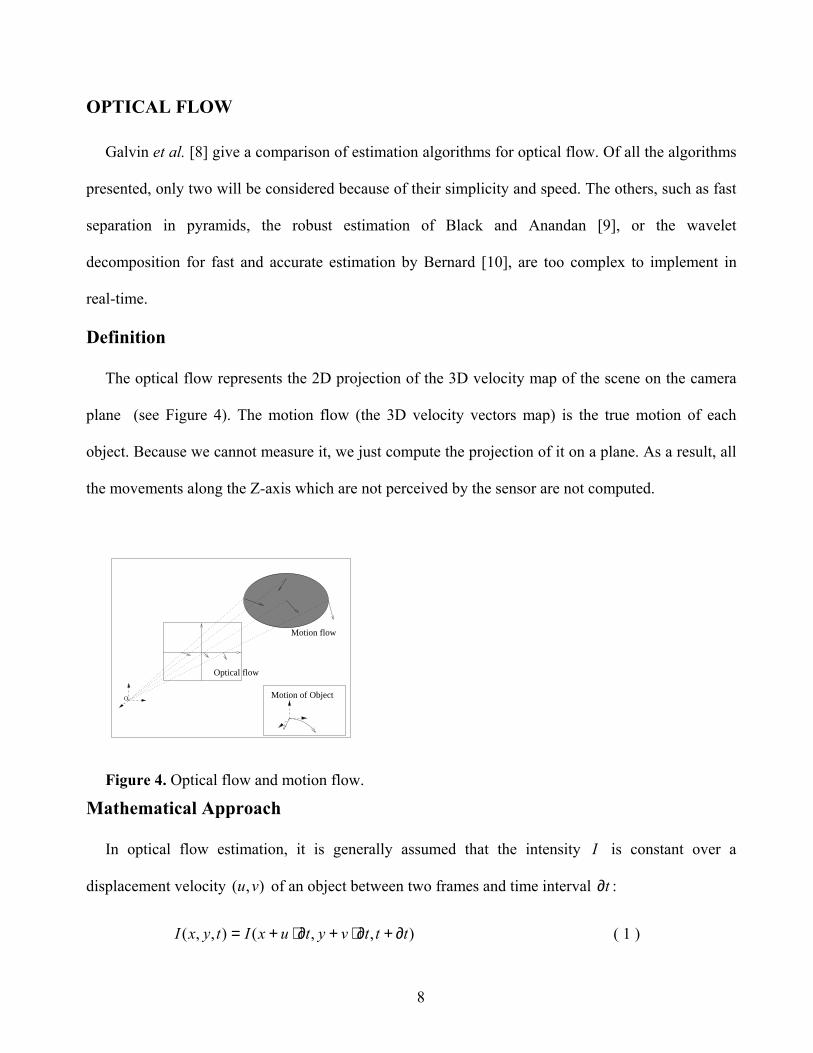
Definition

The optical flow represents the 2D projection of the 3D velocity map of the scene on the camera

plane (see Figure 4). The motion flow (the 3D velocity vectors map) is the true motion of each

object. Because we cannot measure it, we just compute the projection of it on a plane. As a result, all

the movements along the Z-axis which are not perceived by the sensor are not computed.

Motion flow

Optical flow

Motion of ObjectO

Figure 4. Optical flow and motion flow.

Mathematical Approach

In optical flow estimation, it is generally assumed that the intensity I is constant over a

displacement velocity ),( vu of an object between two frames and time interval t∂ :

),,(),,( tttvytuxItyxI ∂+∂⋅+∂⋅+= ( 1 )

9

A Taylor expansion of the right hand side of ( 1 ) gives:

)(),,( tOt

tIv

yIu

xItyxI ∂+∂⋅

∂∂+

∂∂+

∂∂+

( 2 )

Setting ( 1 )=( 2 ), we get the following equation:

0=

∂∂+

∂∂+

∂∂

tIv

yIu

xI

( 3 )

In reality, this equation is not directly applicable due to the lack of constraints on u and v .

Differential Method

This method is explained in Beauchemin and Barron [11]. It was also used by Rwekamp and Peter

[12] with the goal of using ASIC processors for the real-time detection of movement. The idea is to

use a minimization procedure where a spatial estimate of the derivative by a Laplacian is employed.

One may use a spatial iterative filter to obtain a more precise estimation.

We have experimented with this method using a floating point implementation as well as an

integer implementation (for efficiency concerns). Based on our experiments, we concluded that

although this method works well with synthetic images, it is sensitive to noise which is present in our

video sequences. In addition, the computational cost is prohibitive (less than 1 fps in the floating

point implementation). For these reasons, we decided to explore other methods.

Correlation Method

Principle

We look for the velocity vector of each pixel by analyzing its motion between two successive

images: iI and 1−iI . To know the position of the pixel in the next image iI , we calculate a similarity

value on all the possible destinations. This value can be obtained using standard sum-of-squared

differences (SSD) or sum-of-absolute differences (SAD). In all the cases, we have to go through a

10

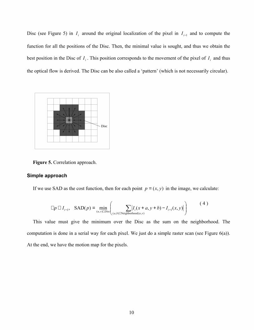
Disc (see Figure 5) in iI around the original localization of the pixel in 1−iI and to compute the

function for all the positions of the Disc. Then, the minimal value is sought, and thus we obtain the

best position in the Disc of iI . This position corresponds to the movement of the pixel of iI and thus

the optical flow is derived. The Disc can be also called a ‘pattern’ (which is not necessarily circular).

Disc

Figure 5. Correlation approach.

Simple approach

If we use SAD as the cost function, then for each point ),( yxp = in the image, we calculate:

−++=∈∀ ∑

∈−∈−

),(odNeighborho),(1),(1 ),(),(min)(SAD,

vubaiiDiscvui yxIbyaxIpIp

( 4 )

This value must give the minimum over the Disc as the sum on the neighborhood. The

computation is done in a serial way for each pixel. We just do a simple raster scan (see Figure 6(a)).

At the end, we have the motion map for the pixels.

11

Next pixel

(a) Raster scan

B CA

A B CDifférence

TmpBuf

Disc

(b) Optimized correlation

Figure 6. Two ways to see the correlation.

Optimized approach

We utilized our hardware (Matrox Genesis vision board) in implementing a parallel version of this

approach. The optimized approach has the following phases:

Phase 1: Parallel calculation of the cost function

Here, we calculate all the differences for a position of the Disc. All the simple arithmetic

operations can be done on sub-windows (child buffers). In our case, we define as many sub-windows

as the number of positions in the Disc. In other words, if the Disc contains N points, we have N

sub-windows gathered in a single TmpBuf buffer array and indexed by their positions. Each one will

contain the result of a subtraction between image iI and the image 1−iI , but with a spatial shift

corresponding to the position of the point in the Disc (see Figure 6(b)).

To do this, we use a sliding window in image iI and a fixed window at the center of image 1−iI .

We compute the difference between these windows, which have the same size, and then we convolve

the difference image with a kernel of ones. Thus, we have the sum and therefore the value of the cost

12

function for this position in the Disc. The result is saved in TmpBuf. Then, we move the window of

image iI to reach another position of the Disc and so on. The kernel can be of size 3x3, 5x5, …,

11x11. The larger it is, the less the noise will be. But that also means less sensitivity. A good

compromise is a size of 5x5 or 7x7.

Phase 2: Retrieval of indices of minimal cost

At the end of the algorithm, we seek the minimum value of the cost function for each pixel

moved. The imaging hardware can calculate the minimum M between two images kI and lI by the

formula:

)),(),,(min(),( jiIjiIjiM lk= ( 5 )

We augment the cost values with indices (locations in Disc) to retrieve the flow.

A last optimization, or rather approximation, is to define a Disc where only the principal axes are

used. We keep for example the horizontal and vertical axes and the diagonals. This approximation is

not restrictive (see Cutler [4]). Also, the radius of Disc itself can be made small. The cameras used

are usually rather far away from the scene and motion does not exceed 2 to 3 pixels per frame.

Therefore, a typical Disc is defined as follows:

1 1 1

1 1 1

1 1 1 1 1

1 1 1

1 1 1

13

Noise removal

To remove the noise from the images during the correlation, thresholding is used. It is known (see

Cutler [4]) that a video CCD camera has a Gaussian white noise of amplitude Kσ with 5.2=σ and

10to5=K according to the model of the camera. In our difference calculation, the conclusion is

that an absolute difference less than σ6 is considered as noise.

As the noise is white, the calculation of the cost function at the central position gives the value of

the noise at each pixel. Moreover, after convolution, this noise is averaged. A thresholding with

2KernelKS ⋅⋅= σ gives a mask corresponding to the level of noise. Thus, the points that give a

lower value than this level are not to be taken into account at our optical flow estimate. For example

with a kernel 5x5, we obtain 375565.2 2 =⋅⋅=S .

Results

The results are very good for the estimation part. The kernel that was used for the summation is

7x7. On 320x240 images with a Disc of 3± pixels, the processing rate is approximately 4 fps. On

160x120 images and by using the same Disc, we reached computational speeds of 10 fps.

Conclusion for our application

This method is very adaptable to our problem. The limitation of the size of the Disc does not

prevent it from having a good separation between moving parts and noise. It is a robust and fast

method; we reach the 15 fps with a Disc radius of 2± pixels.

14

BACKGROUND

To detect the static traffic objects or people, we need another way for approaching the problem.

For these cases, we use a detection scheme that subtracts the image from the background. The idea is

based on an adaptive background update. The update equations are as follows:

( )

),(OR

)(NOT,16

15AND

,AND

bkgnd

mask opt.bkgndframecurrent

mask opt.bkgnd

BAM

IMI

B

IMA

=

⋅+=

=

( 6 )

where bkgndM is the background, framecurrent I is the current image, and mask opt.I is the mask obtained

after binarization of the optical flow. Every 16 iterations, the background is completely readjusted.

The detection is carried out at every new estimation of the optical flow by a simple subtraction of

the background and thresholding with Kσ4 (a value much higher than the one for the flow). Then,

we merge the results obtained by these two methods by assigning the background a special value

(meaning that the blob comes from the second type of detection and not from the optical flow). The

estimation of the optical flow is dominating on the background (in the case of double detection). That

processing leads to a unified color map mixing the two methods and having a lookup table describing

the motion and the nature of each point. The points belonging to the background are associated to no

motion and no position in the Disc.

SEGMENTATION

The segmentation is the next step. In our case, the choice of an effective method is not obvious.

The goal is to use some information from this stage during the tracking phase.

15

Clustering the Motion Map from the Optical flow

For this simple stage, we have various choices: a raster scan, a border following or a floodfill

algorithm. Figure 7 shows the three methods.

(a) Raster Scan (b) Border Following (c) Floodfill

Figure 7. Classic methods for segmentation.

Raster scan

This method is very effective for zone segmentation and detection in the case of large shapes that

may have holes. The algorithm consists of dividing the image into runs and memorizing the similar

parts in a run. It is very fast and the computational time is only dependent on the size of the image,

not its content. On the other hand, it requires two passes to obtain the segmentation and it must

maintain a chain-list of runs. Therefore, it has a high memory requirement that need to be

appropriately managed to guarantee sufficient speed. Statistics relating to the zones (e.g., size, area,

the minimal bounding rectangle, the mean velocity estimated by the flow) can be calculated on the

fly and do not require additional stages. We just have to go through the chain-list of runs to gather the

data.

16

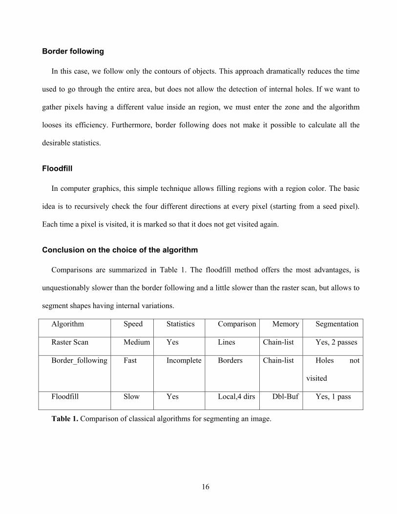
Border following

In this case, we follow only the contours of objects. This approach dramatically reduces the time

used to go through the entire area, but does not allow the detection of internal holes. If we want to

gather pixels having a different value inside an region, we must enter the zone and the algorithm

looses its efficiency. Furthermore, border following does not make it possible to calculate all the

desirable statistics.

Floodfill

In computer graphics, this simple technique allows filling regions with a region color. The basic

idea is to recursively check the four different directions at every pixel (starting from a seed pixel).

Each time a pixel is visited, it is marked so that it does not get visited again.

Conclusion on the choice of the algorithm

Comparisons are summarized in Table 1. The floodfill method offers the most advantages, is

unquestionably slower than the border following and a little slower than the raster scan, but allows to

segment shapes having internal variations.

Algorithm Speed Statistics Comparison Memory Segmentation

Raster Scan Medium Yes Lines Chain-list Yes, 2 passes

Border_following Fast Incomplete Borders Chain-list Holes not

visited

Floodfill Slow Yes Local,4 dirs Dbl-Buf Yes, 1 pass

Table 1. Comparison of classical algorithms for segmenting an image.

17

Two Features Computed by the Segmentation

Rotation

When an object is in slow rotational motion, the pixels describing the object move according to a

local gradient. Each point has a direction slightly different from its neighbor. Therefore, if the

rotation is not fast, the floodfill algorithm helps us gather all these close pixels. In this method, we

adjust a validation parameter: the maximum angle between two directions. To calculate the

difference between two angles, the following formula is used:

−>−−−

=otherwise

if

21

2121

AngleAngle180AngleAngleAngleAngle360

difference

(7 )

This approach also helps maintain all the pixels which are static.

Shape fitting

After the segmentation, the blobs are shaped into simple geometrical shapes. At this stage, a

minimum bounding box can be calculated. The floodfill algorithm makes the procedure easier since it

provides all the points contained in the shape. At the end of the segmentation, the blobs are described

by the minimum bounding box, the position of their centers, and the number of pixels they contain

(or mass). A better adaptation to a more complex shape can be carried out at this stage (oriented

bounding box) and will be explained later.

18

19

CHAPTER 3 TRACKING

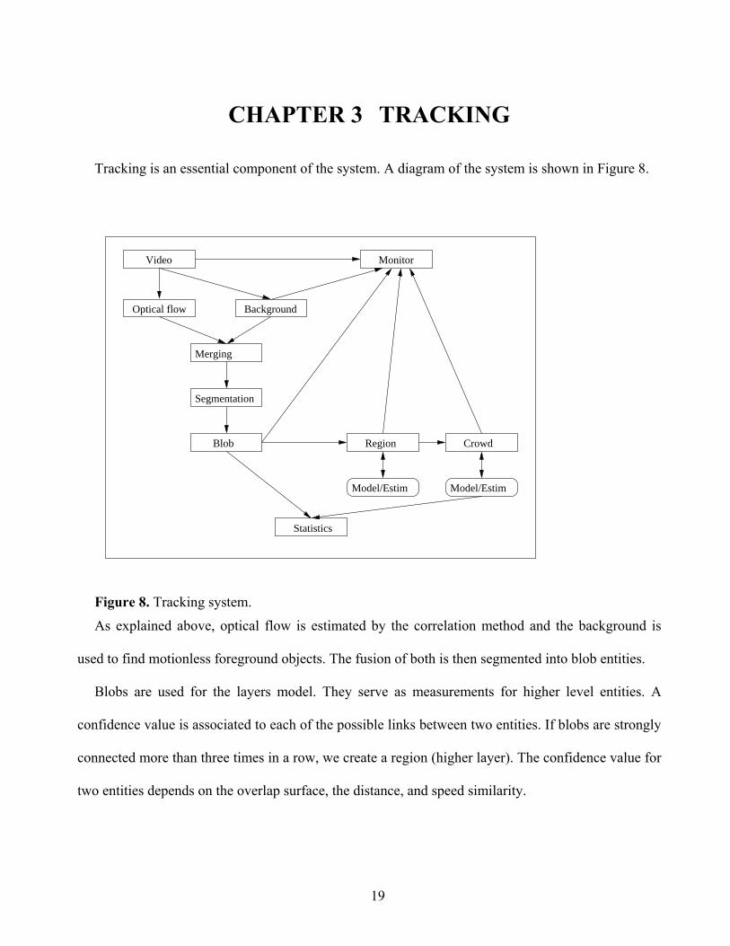
Tracking is an essential component of the system. A diagram of the system is shown in Figure 8.

Background

Merging

Segmentation

Blob

Monitor

Statistics

Video

Optical flow

Region Crowd

Model/Estim Model/Estim

Figure 8. Tracking system.

As explained above, optical flow is estimated by the correlation method and the background is

used to find motionless foreground objects. The fusion of both is then segmented into blob entities.

Blobs are used for the layers model. They serve as measurements for higher level entities. A

confidence value is associated to each of the possible links between two entities. If blobs are strongly

connected more than three times in a row, we create a region (higher layer). The confidence value for

two entities depends on the overlap surface, the distance, and speed similarity.

20

LAYER MODEL

First Level: Blobs

We model a blob using its position, size, area, and velocity. The first three parameters are

computed by the floodfill algorithm during segmentation. If we add a pixel, ),( yxP , to the blob, we

have:

Size

Let Size be an accumulator. So each time we add a pixel, we do: 11 += −nn SizeSize

Position

Let cX , cY be accumulators. We define their sum by:

+=+=

−

−

yYYxXX

cncn

cncn

1

1 ( 8 )

Then at the end of the floodfill, we compute the centroid using the first moment:

=

=

SizeY

YSizeX

X

cnc

cnc

σ

σ

( 9 )

Velocity

Let xV , yV be accumulators. Since pixel velocity is stored as an index into Disc, we get its

displacement xD , yD by looking up the pattern:

+=+=

==

−

−

yynyn

xxnxn

y

x

DVVDVV

yxPDyxPD

1

1 thenAnd)],(ntY[Displaceme)],(ntX[Displaceme ( 10 )

21

Then, we have the global velocity of the blob:

=

=

SizeV

V

SizeV

V

yny

xnx

σ

σ

( 11 )

Area (minimum bounding box)

Let MinX, MaxX, MinY, and MinY be values of the sides of the box. We have:

x)MinX,min(MinX = , x)MaxX,max(MaxX = , and similarly for MinY and MaxY. This, we have

Area=( MaxX-MinX) *(MaxY-MinY).

These blobs describe all zones in the optical flow. Their modeling is easy and fast. The floodfill

algorithm is needed here if we want to have that kind of description.

Second Level: Regions

The intrinsic parameters are the same as for the blobs. The differences are in the way we compute

their values. The regions inherit values from their parent blobs at their creation but they are adapted

during the tracking. Other properties, like the time of existence or inactivity, are also used for

regions.

GEOMETRICAL DESCRIPTION OF THE ENTITIES

The tracking part has been improved by the introduction of new blob descriptions. Relations based

on simple bounding boxes are clearly not effective for very mobile and close objects (such as distant

pedestrians). Moreover, the density ( AreaMass ) of a crowd is badly represented by this approach.

22

Therefore, we compute oriented rectangles instead of horizontally aligned boxes. We want to

preserve simplicity and efficient computation of these shapes.

Oriented Boxes

Covariance Matrix

For a 2-D space of n points, we have a covariance matrix M between the two variables X and

Y . It is defined by:

><><><><

= 2

2

,,

YYXYXX

M ( 12 )

The marks <> mean that we take the variance value.

Eigenspace representation

We use a technique often associated with the principal components analysis: the diagonalization

reduction. This representation results in finding maximum dispersions by analyzing eigenvalues and

eigenvectors. Given M , its decomposition is written as: ∆∆= DM t , with ∆ being the transition

matrix, and D the diagonal matrix with eigenvalues. Let [ ]21 ,vv=∆ and

=

2

1

00e

eD . We can

choose to have 21 ee > , so that 1v gives the direction of elongation and 1e gives the total

elongation. The second axis is described by 2v and 2e .

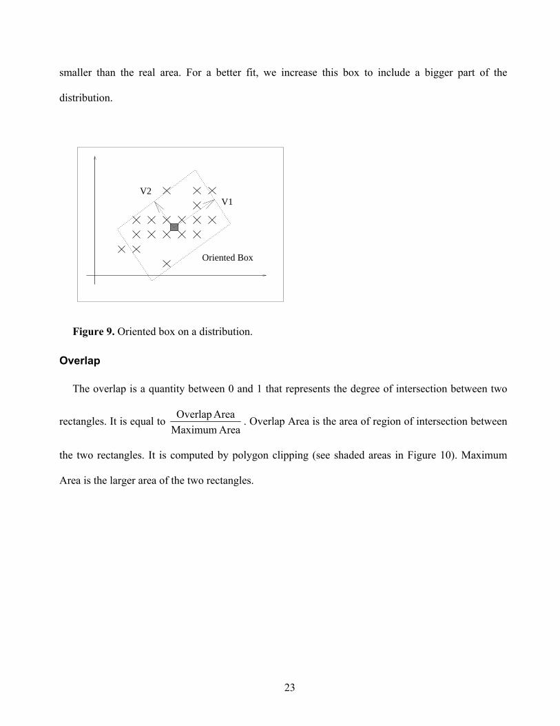
For example, Figure 9 describes a two-dimensional distribution. Using this scheme, the two

vectors and the resulting rectangle are shown. In our algorithm, we include a multiplicative

coefficient equal to 1.5 for the two sides. The elongation obtained after diagonalization is often a box

23

smaller than the real area. For a better fit, we increase this box to include a bigger part of the

distribution.

V2V1

Oriented Box

Figure 9. Oriented box on a distribution.

Overlap

The overlap is a quantity between 0 and 1 that represents the degree of intersection between two

rectangles. It is equal to Area Maximum

Area Overlap . Overlap Area is the area of region of intersection between

the two rectangles. It is computed by polygon clipping (see shaded areas in Figure 10). Maximum

Area is the larger area of the two rectangles.

24

Figure 10. Overlap Area.

DETAILS OF RELATIONS

All the relations are based on confidence values ),( βα which reflect the similarity between two

entities A and B . We introduce thresholds to define the presence or absence of a relation between

two entities. In our tracker, the value α will be related to the position and the area of the objects

while the value β will be related to the similarity in motion direction deduced from optical flow.

Our merging algorithm is based on a score calculation between entities.

Relations Based on Scores

We propose to create a tracking method based on scores of each blob iB with regard to a region

A . Then, we keep only a percentage of the best related blobs that we use in a Kalman filter as

measurement. The introduced score will be used as confidence value for the filtering.

Score dependent on position

During this phase, we have the positions and descriptions for blobs and regions. First, we compute

the distance with a fuzzy model using the distance between the two centroids and the perimeter of

each rectangle. We introduce a confidence term by normalizing the distance by a multiple of the

25

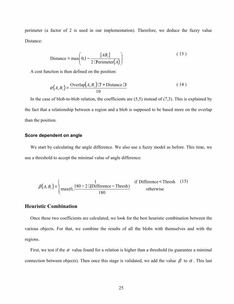
perimeter (a factor of 2 is used in our implementation). Therefore, we deduce the fuzzy value

Distance:

( )

⋅−=

AABi

Perimeter21,0maxDistance

( 13 )

A cost function is then defined on the position:

( ) ( )10

3Distance7,Overlap,

⋅+⋅= i

iBA

BAα ( 14 )

In the case of blob-to-blob relation, the coefficients are (5,5) instead of (7,3). This is explained by

the fact that a relationship between a region and a blob is supposed to be based more on the overlap

than the position.

Score dependent on angle

We start by calculating the angle difference. We also use a fuzzy model as before. This time, we

use a threshold to accept the minimal value of angle difference:

( )

−⋅−<

= otherwise180

)ThreshDifference(2180,0max(Thresh Difference if1

, iBAβ

(15)

Heuristic Combination

Once these two coefficients are calculated, we look for the best heuristic combination between the

various objects. For that, we combine the results of all the blobs with themselves and with the

regions.

First, we test if the α value found for a relation is higher than a threshold (to guarantee a minimal

connection between objects). Then once this stage is validated, we add the value β to α . This last

26

value provides the final cost function for the relations. All the entities (regions or blobs) are tested

and the relationships are calculated. Then, we keep the group of the best relationships.

Regions creation based on blob-to-blob relationships

During each loop, we preserve the previous list of blobs to check which of the new blobs are

related to the preceding ones. These relationships are one-to-one. A counter on each previous entity

specifies if a link has already been created before. The counter is propagated from one entity to

another and thus gives the total number of blobs related in a row. If this value exceeds a threshold (2

in our case), then we create a new region inheriting the parameters of the last linked blob. The

minimal threshold is taken such that we have at least %50>α in each relation.

Merging many blobs

The relationships between blobs and regions are many-to-many. In other words, several blobs can

be used as measurements for a region. A threshold, %10>α , ensures a minimal relationship. Then,

we create a list of the relationships ranging between 70% of the maximum value and the maximum

value itself. This group of blobs will be used to estimate the location measurement of the region at

the next loop. For this, we compute the centroid, the minimal bounding box, and the mean velocity of

the group. Then, we use this information in the regions measurement/estimation part (filtering).

STATE SPACE REPRESENTATION OF REGIONS

State Vector and Data Splitting

The positions x and y are related to the region centroid. The other parameters are the covariances

and the mass (number of pixels).

27

We can describe all regions by a state representation: let X be the state vector that describes a

region:

><><><

=

mass,cov

covcov

2

2

yxyx

yyxx

&

&

X

( 16 )

So our system has the following state equation:

VXX +⋅

∆

∆

=′

10000000010000000010000000010000000010000000100000000100000001

t

t

( 17 )

The parameters are only estimated and do not have real physical significance. The measurement

equation is:

WXCY +⋅= ( 18 )

with:

=

100000000100000000100000000100000000010000000001

C

( 19 )

28

Position Characteristics

We use a constant velocity model for the coordinates,

=

yyxx

&

&X

( 20 )

and,

1

1000100

0010001

VXX +⋅

∆

∆

=′t

t

( 21 )

1V is a white Gaussian noise that depends on the system. Its covariance has a matrix that has an

estimate for limit. In our case:

{ }

=

⋅→

y

y

x

x

TT

&

&

σσσσ

ε

position

positionposition11,

V

VVVV

( 22 )

The equation yx σσ = shows the system's standard-deviation in position while yx && σσ = shows the

one in velocity.

Shape Features

In the same way, we obtain:

2

param)(VXX

X+=′

=

( 23 )

2V is a white Gaussian noise that depends on the feature. Its covariance has an estimate for limit:

29

{ }paramparam

param2

σε

=→

VVV

( 24 )

KALMAN FILTERING

The Kalman filter makes it possible to merge measurements assuming that we know their

reliability. Furthermore, it allows to optimally estimate the next state of the system. The process to be

estimated must be controlled by a differential equation, linear and stochastic. We will not extend on

the subject since our study requires only a first order filter. Our formulas are laid out in the following

sections.

Position Filtering

Measurement equations:

Kalman gain:

( ) 1ˆˆ −+⋅⋅⋅⋅= n

Tn

Tnn RCPCCPK ( 25 )

State correction:

( )nnnnn XCYKXX ˆˆ ⋅−⋅+= ( 26 )

Variance:

nnn P)K(IP ˆ⋅−= ( 27 )

Temporal equations:

System:

nn XAX ⋅=+1

ˆ ( 28 )

Variance propagation:

30

n

Tnn QAPAP +⋅⋅=+1

ˆ ( 29 )

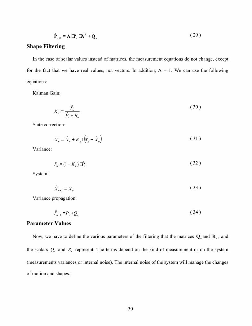
Shape Filtering

In the case of scalar values instead of matrices, the measurement equations do not change, except

for the fact that we have real values, not vectors. In addition, A = 1. We can use the following

equations:

Kalman Gain:

nn

nn RP

PK+

= ˆˆ

( 30 )

State correction:

( )nnnnn XYKXX ˆˆ −⋅+= ( 31 )

Variance:

nnn PKP ˆ)1( ⋅−= ( 32 )

System:

nn XX =+1

ˆ ( 33 )

Variance propagation:

nnn QPP +=+1

ˆ ( 34 )

Parameter Values

Now, we have to define the various parameters of the filtering that the matrices nQ and nR , and

the scalars nQ and nR represent. The terms depend on the kind of measurement or on the system

(measurements variances or internal noise). The internal noise of the system will manage the changes

of motion and shapes.

31

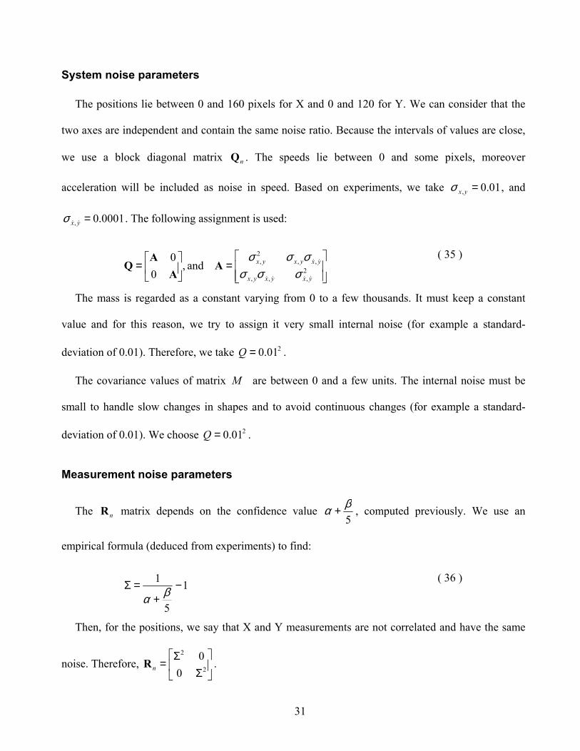
System noise parameters

The positions lie between 0 and 160 pixels for X and 0 and 120 for Y. We can consider that the

two axes are independent and contain the same noise ratio. Because the intervals of values are close,

we use a block diagonal matrix nQ . The speeds lie between 0 and some pixels, moreover

acceleration will be included as noise in speed. Based on experiments, we take 01.0, =yxσ , and

0001.0, =yx &&σ . The following assignment is used:

=

= 2

,,,

,,2,and ,

00

yxyxyx

yxyxyx

&&&&

&&

σσσσσσ

AA

AQ

( 35 )

The mass is regarded as a constant varying from 0 to a few thousands. It must keep a constant

value and for this reason, we try to assign it very small internal noise (for example a standard-

deviation of 0.01). Therefore, we take 201.0=Q .

The covariance values of matrix M are between 0 and a few units. The internal noise must be

small to handle slow changes in shapes and to avoid continuous changes (for example a standard-

deviation of 0.01). We choose 201.0=Q .

Measurement noise parameters

The nR matrix depends on the confidence value 5βα + , computed previously. We use an

empirical formula (deduced from experiments) to find:

1

5

1 −+

=Σ βα

( 36 )

Then, for the positions, we say that X and Y measurements are not correlated and have the same

noise. Therefore,

ΣΣ

= 2

2

00

nR .

32

For the state parameters, we found that Σ=nR gives good results.

Initialization

We initialize the filtering at the current position of the region and a zero speed, because the value

obtained by the optical flow is not accurate enough at this stage. The matrix 0P is reset to zero. The

intrinsic characteristics are initialized with the current region values and 0P is set to zero.

33

CHAPTER 4

RESULTS AND CONCLUSIONS

We tried our algorithms in several outdoor scenes from the Twin Cities area. One area where one

may find crowds is around the Xcel Energy Center in St Paul. We filmed scenes during day and

night. We also applied our method on a video during winter at a road intersection to check the quality

of the tracking when vehicles drive past each other in opposite directions. The optical flow and the

first layer (blobs) give the required statistics on crowds: direction, size, and mean velocity.

GENERAL COMMENTS

The speed of our software depends on the quality of the detection done by the optical flow

approach. In the general case, a Disc with a radius of 1 pixel is enough to detect objects on images

with size of 160x120 pixels. All the results are obtained with a 5x5 Kernel, which allows a very good

detection without significant corruption by noise. Then, our tracker runs at 15 fps with all the

characteristics displayed on 4 different screen buffers on the same monitor: optical flow map,

background, tracked regions, and most used zone. If we increase the detection with a Disc of radius

2, the frame rate drops to 10 fps. Here, we should mention the following observation for the quality

of the tracking. One thing worth mentioning is that in case some frames have to be dropped, it is

important to drop the same number of frames consistently. For example, the pattern would be one

frame processed followed by two dropped and so on. Otherwise we get temporal instability. The

reason is that optical flow estimation assumes that the time interval between two frames is always the

34

same. For this reason, our tracker runs at speeds of either 15 fps or 10 fps, or 1

30+n

fps (n being the

number of skipped frames).

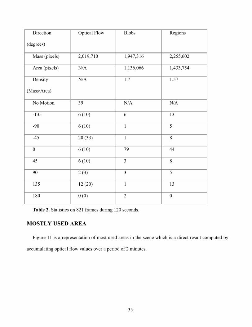
STATISTICS

The first result we present shows statistics gathered over a period of time 2=T minutes. These

statistics were computed from optical flow, blobs, and regions. The values are shown in Table 2. The

statistics were computed by accumulating the flow, region, and blob directions during T . In the case

of optical flow, the table shows the percentage of pixels moving in different directions (the values in

parenthesis show the percentage out of moving pixels only). In the case of blobs (and regions), the

percentages are also of pixels but the directions are of blobs (and regions) containing these pixels.

The frame rate was 10 fps. Notice that blobs were not able to sufficiently capture the motion in

direction 135. This is due to the fact that blobs may be accurately initialized in terms of direction

when the underlying motion of pixels is not consistent. This also stresses the need for the regions

level which was able to capture that direction based on blob information even though the information

is not accurate. Notice also that the most frequent region direction is 0 whereas the most frequent

pixel direction is –45. This is merely a quantization issue since pixel directions are quantized while

region directions are not.

The density represents the ratio of the number of pixels in a blob (or region) to the area of the

bounding box of the blob (or region). This value exceeds 1 because of inaccuracies of modeling the

blob (or region) as a rectangle. However, it is a useful indicator to identify a crowd; a region

representing a crowd would have a high density (above 0.75). Other parameters that can be used to

identify a crowd are the area (sufficiently large) and the speed (sufficiently small).

35

Direction

(degrees)

Optical Flow Blobs Regions

Mass (pixels) 2,019,710 1,947,316 2,255,602

Area (pixels) N/A 1,136,066 1,433,754

Density

(Mass/Area)

N/A 1.7 1.57

No Motion 39 N/A N/A

-135 6 (10) 6 13

-90 6 (10) 1 5

-45 20 (33) 1 8

0 6 (10) 79 44

45 6 (10) 3 8

90 2 (3) 3 5

135 12 (20) 1 13

180 0 (0) 2 0

Table 2. Statistics on 821 frames during 120 seconds.

MOSTLY USED AREA

Figure 11 is a representation of most used areas in the scene which is a direct result computed by

accumulating optical flow values over a period of 2 minutes.

36

Figure 11. Mostly used areas during two minutes of day video.

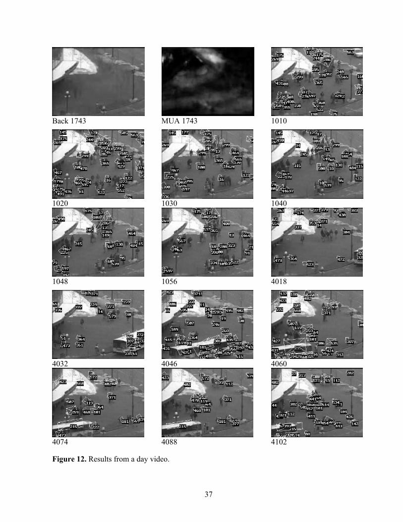
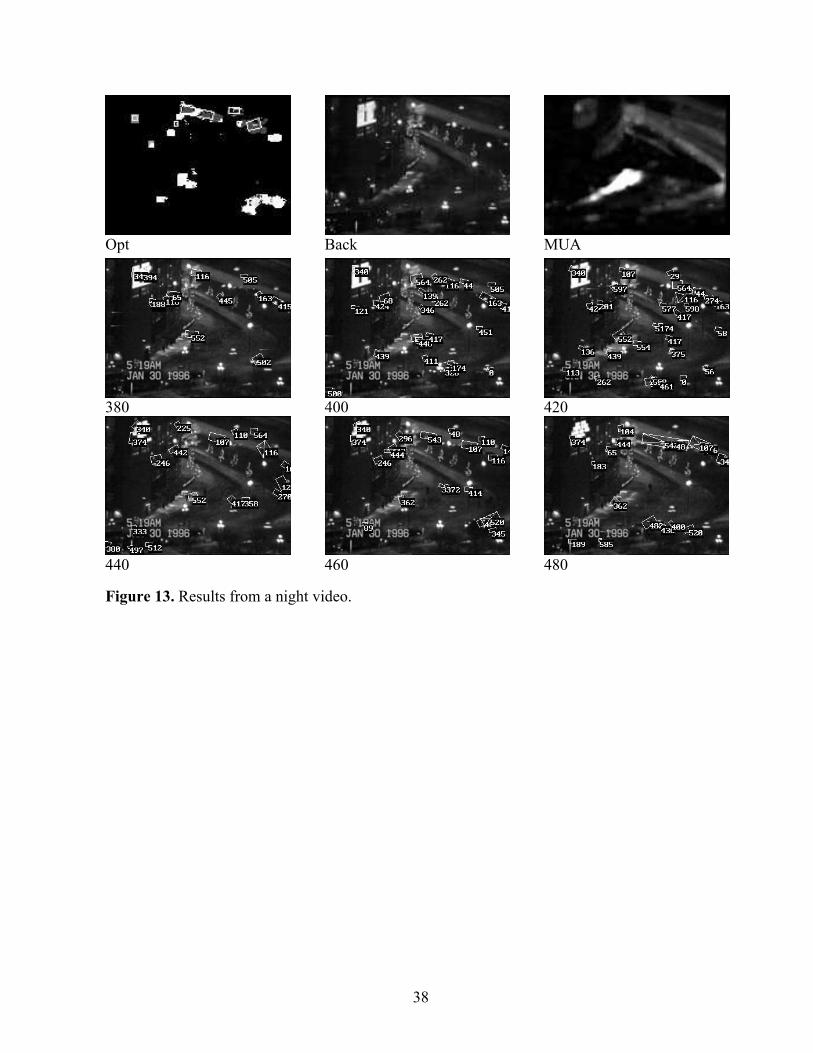
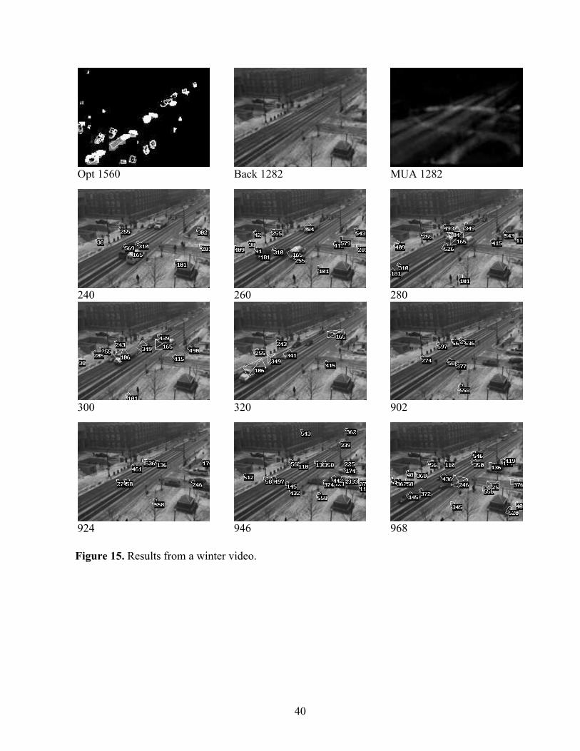
TRACKING RESULTS

Figure 12, Figure 13, Figure 14, and Figure 15 show some of the tracking results. The results are

presented as snapshots every 2 seconds. Rectangles represent regions. Regions with a cross represent

detected crowds. The numbers shown are the region identifiers. Images marked ‘Back’ are

background. Images marked ‘MUA’ show mostly used areas. Images marked ‘Opt’ show optical

flow and optical flow segmentation.

CONCLUSIONS

This paper presents a vision-based system for monitoring crowded urban scenes. Our approach

employs an effective detection scheme based on optical flow that can locate vehicles, individual

pedestrians, and crowds. The detection phase is followed by the tracking phase that tracks all the

detected entities. Traffic objects are not simply tracked but a wealth of information is gathered about

them (position, velocity, acceleration/deceleration, bounding box, and shape features). Potential

applications of our methods include intersection control, traffic data collection, and even crowd

control after athletic events. Extensive experimental results for a variety of weather conditions are

presented. Future work will be focused on methods to deal with shadows and occlusions.

37

Back 1743 MUA 1743

1010

1020

1030

1040

1048

1056

4018

4032

4046

4060

4074

4088

4102

Figure 12. Results from a day video.

38

Opt

Back MUA

380

400

420

440

460

480

Figure 13. Results from a night video.

39

4278 4290

4302

4314 4326

4338

4350 4362

4374

7273 7280

7287

7294 7301

7308

Figure 14. Results from a real-time video.

40

Opt 1560 Back 1282

MUA 1282

240

260

280

300

320

902

924

946

968

Figure 15. Results from a winter video.

41

CHAPTER 5 REFERENCES

[1] A. Baumberg and D. Hogg, 'An Efficient Method for Contour Tracking Using Active Shape Models', in Proc. of IEEE Workshop on Motion of Non-rigid and Articulated Objects, pp. 195-199, IEEE Computer Society Press, November 1994.

[2] M. Rossi and A. Bozzoli, 'Tracking and Counting Moving People', Proc. Second IEEE International Conference on Image Processing, pp. 212-216, 1994.

[3] O. Masoud, Ph.D. Thesis on 'Tracking and Analysis of Articulated Motion with an Application to Human Motion', University of Minnesota, Minneapolis, March 2000.

[4] R. Cutler and M. Turk, 'View-based Interpretation of Real-time Optical Flow for Gesture Recognition', Third IEEE International Conference on Automatic Face and Gesture Recognition, Nara, Japan, April 14-16, 1998.

[5] S. L. Dockstader, 'Motion Estimation and Tracking', University of Rochester, document on the web, http://www.ee.rochester.edu:8080/users/dockstad/research/rtop.html, May 24, 2001.

[6] I. Haritaoglu, D. Harwood, and L.S. Davis, 'Real-Time Surveillance of People and Their Activities', IEEE Transactions on Pattern Analysis and Machine Intelligence, vol. 22, no. 8, pp. 809-830, August 2000.

[7] C. Sun, 'A Fast Stereo Matching Method', Digital Image Computing: Techniques and Applications, pp.95-100, Massey University, Auckland, New Zealand, December 10-12, 1997.

[8] B. Galvin, B. McCane, K. Novins, D. Mason, and S. Mills, 'Recovering Motion Fields: An Evaluation of Eight Optical Flow Algorithms', British Conference on Computer Vision, Computer Science Department University of Otago, New Zealand.

[9] M.J. Black and P. Anandan, 'A Framework for the Robust Estimation of Optical Flow', Proc. Fourth Int. Conf. on Computer Vision (ICCV'93), Berlin, Germany, May 1993.

[10] C. Bernard, Ph.D. Thesis on 'Ill-conditioned Problems: Optical Flow and Irregular Interpolation', document on the web, www.cmap.polytechnique.fr/~bernard/these, 1999.

42

[11] S.S. Beauchemin and J.L. Barron, 'The Computation of Optical Flow', Dept. of Computer Science, University of Western Ontario, ACM Computer Surveys, vol. 27, no. 3, pp. 433-467, 1995.

[12] T. Rwekamp and L. Peter, 'A Compact Sensor for Visual Motion Detection', VIDERE, vol. 1, no. 2, Article 2, MIT Press, Winter 1998.