Embed Size (px)
Citation preview
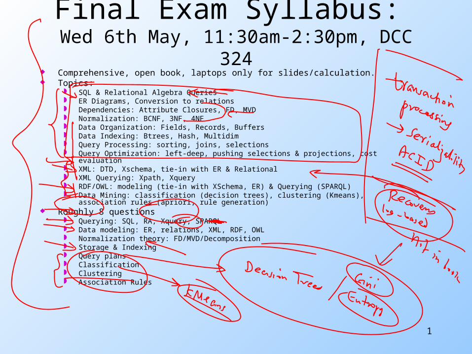
Final Exam Syllabus: Wed 6th May, 11:30am-2:30pm, DCC 324
Comprehensive, open book, laptops only for slides/calculation. Topics:
SQL & Relational Algebra Queries ER Diagrams, Conversion to relations Dependencies: Attribute Closures, FD, MVD Normalization: BCNF, 3NF, 4NF Data Organization: Fields, Records, Buffers Data Indexing: Btrees, Hash, Multidim Query Processing: sorting, joins, selections Query Optimization: left-deep, pushing selections & projections, cost evaluation XML: DTD, Xschema, tie-in with ER & Relational XML Querying: Xpath, Xquery RDF/OWL: modeling (tie-in with XSchema, ER) & Querying (SPARQL) Data Mining: classification (decision trees), clustering (Kmeans), association rules
(apriori, rule generation) Roughly 8 questions
Querying: SQL, RA, Xquery, SPARQL Data modeling: ER, relations, XML, RDF, OWL Normalization theory: FD/MVD/Decomposition Storage & Indexing Query plans Classification Clustering Association Rules
1
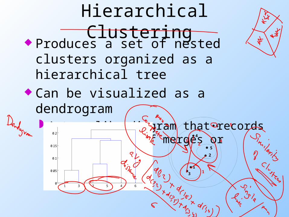
Hierarchical Clustering Produces a set of nested clusters
organized as a hierarchical tree Can be visualized as a dendrogram
A tree like diagram that records the sequences of merges or splits
1 3 2 5 4 60
0.05
0.1
0.15
0.2
1
2
3
4
5
6
1
23 4
5
Strengths of Hierarchical Clustering
Do not have to assume any particular number of clusters Any desired number of clusters can be
obtained by ‘cutting’ the dendogram at the proper level
They may correspond to meaningful taxonomies Example in biological sciences (e.g.,
animal kingdom, phylogeny reconstruction, …)
Hierarchical Clustering Two main types of hierarchical clustering
Agglomerative: • Start with the points as individual clusters• At each step, merge the closest pair of clusters until only
one cluster (or k clusters) left
Divisive: • Start with one, all-inclusive cluster • At each step, split a cluster until each cluster contains a
point (or there are k clusters)
Traditional hierarchical algorithms use a similarity or distance matrix Merge or split one cluster at a time
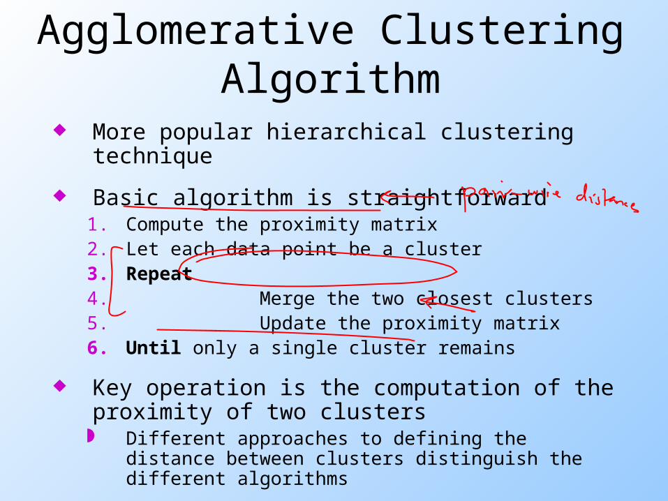
Agglomerative Clustering Algorithm
More popular hierarchical clustering technique
Basic algorithm is straightforward1. Compute the proximity matrix2. Let each data point be a cluster3. Repeat4. Merge the two closest clusters5. Update the proximity matrix6. Until only a single cluster remains
Key operation is the computation of the proximity of two clusters Different approaches to defining the distance
between clusters distinguish the different algorithms
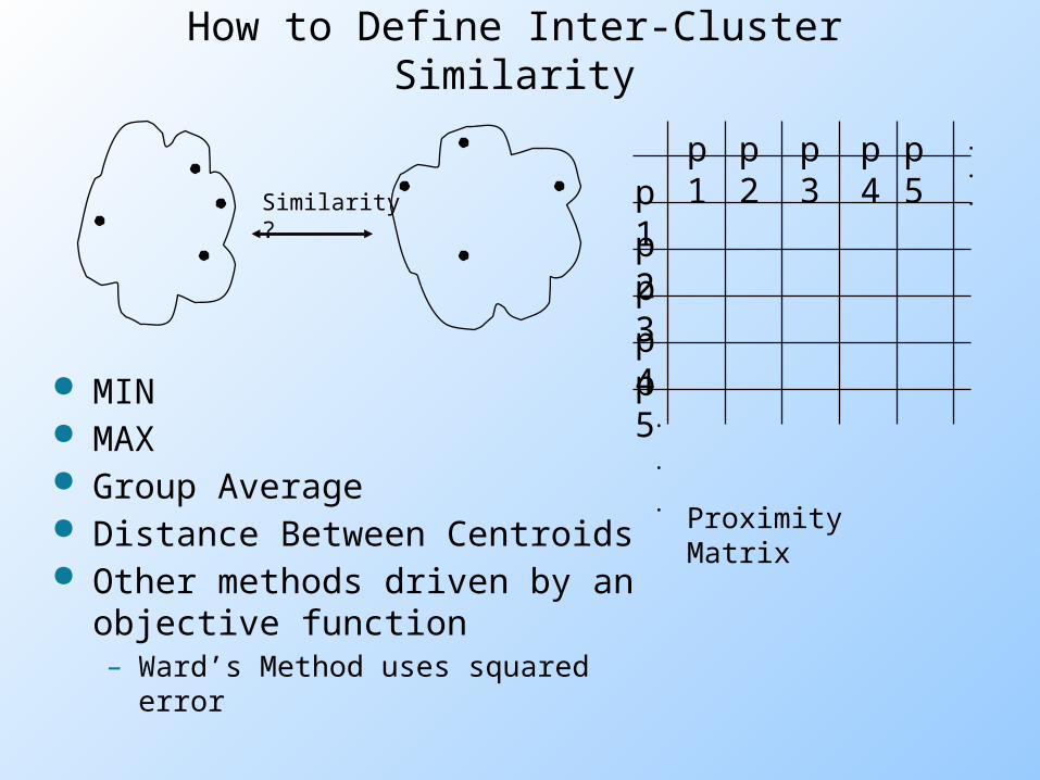
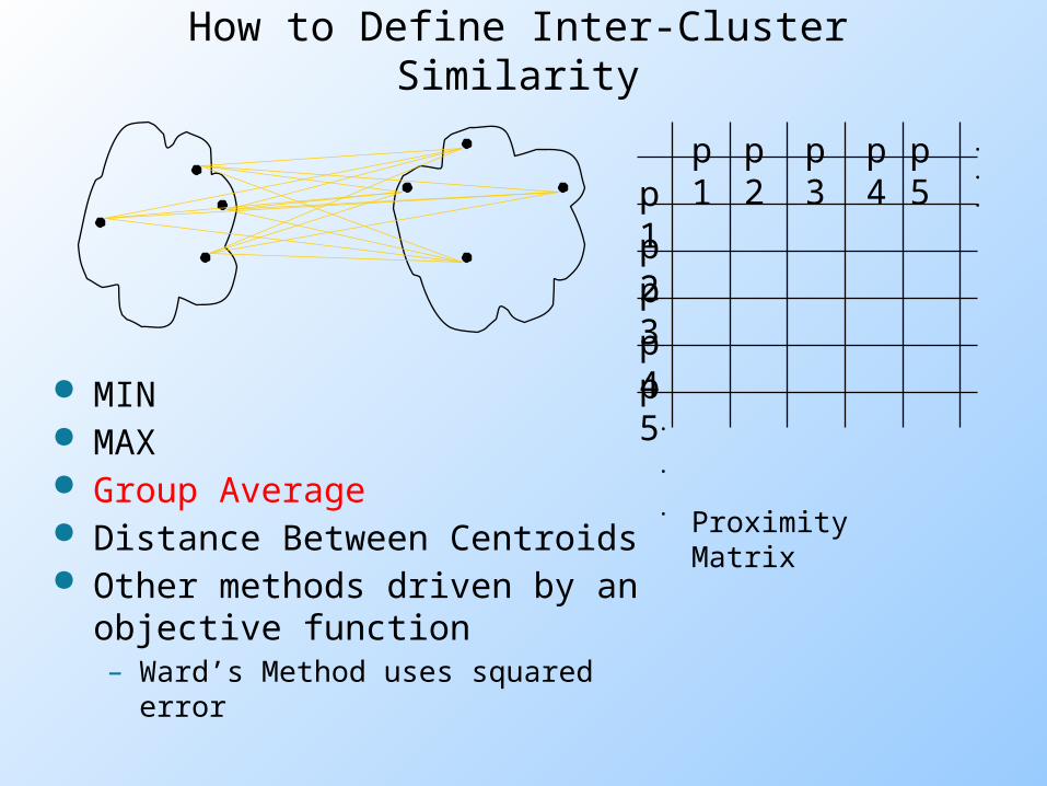
How to Define Inter-Cluster Similarity
p1
p3
p5
p4
p2
p1
p2
p3
p4
p5
. . .
.
.
.
Similarity?
MIN MAX Group Average Distance Between Centroids Other methods driven by an
objective function– Ward’s Method uses squared error
Proximity Matrix
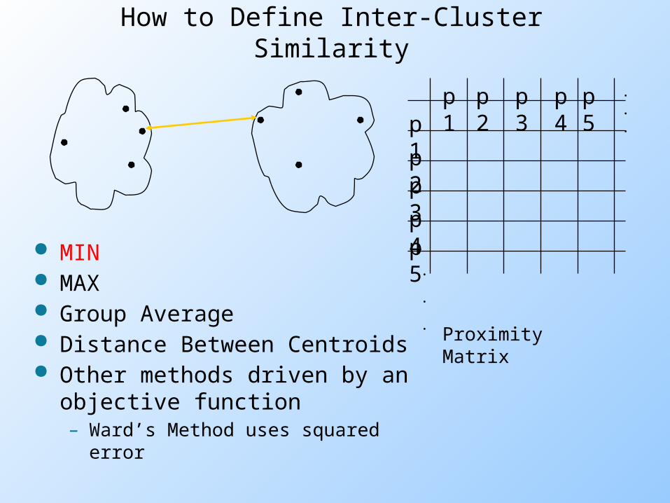
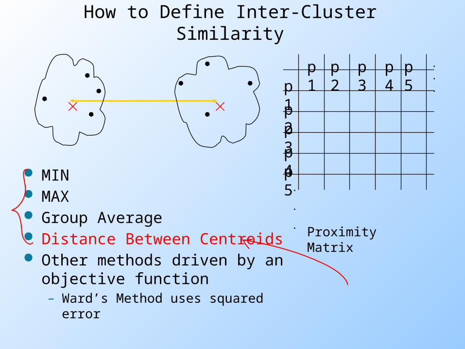
How to Define Inter-Cluster Similarity
p1
p3
p5
p4
p2
p1
p2
p3
p4
p5
. . .
.
.
.Proximity Matrix
MIN MAX Group Average Distance Between Centroids Other methods driven by an
objective function– Ward’s Method uses squared error
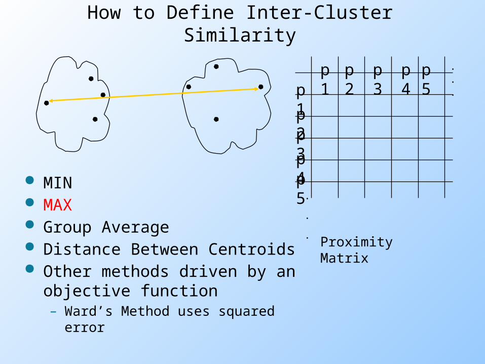
How to Define Inter-Cluster Similarity
p1
p3
p5
p4
p2
p1
p2
p3
p4
p5
. . .
.
.
.Proximity Matrix
MIN MAX Group Average Distance Between Centroids Other methods driven by an
objective function– Ward’s Method uses squared error
How to Define Inter-Cluster Similarity
p1
p3
p5
p4
p2
p1
p2
p3
p4
p5
. . .
.
.
.Proximity Matrix
MIN MAX Group Average Distance Between Centroids Other methods driven by an
objective function– Ward’s Method uses squared error
How to Define Inter-Cluster Similarity
p1
p3
p5
p4
p2
p1
p2
p3
p4
p5
. . .
.
.
.Proximity Matrix
MIN MAX Group Average Distance Between Centroids Other methods driven by an
objective function– Ward’s Method uses squared error
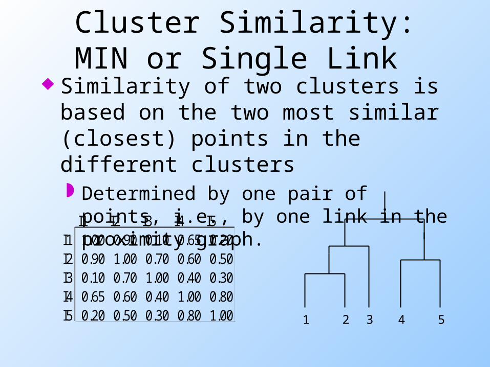
Cluster Similarity: MIN or Single Link
Similarity of two clusters is based on the two most similar (closest) points in the different clusters Determined by one pair of points, i.e.,
by one link in the proximity graph.I1 I2 I3 I4 I5
I1 1.00 0.90 0.10 0.65 0.20I2 0.90 1.00 0.70 0.60 0.50I3 0.10 0.70 1.00 0.40 0.30I4 0.65 0.60 0.40 1.00 0.80I5 0.20 0.50 0.30 0.80 1.00 1 2 3 4 5
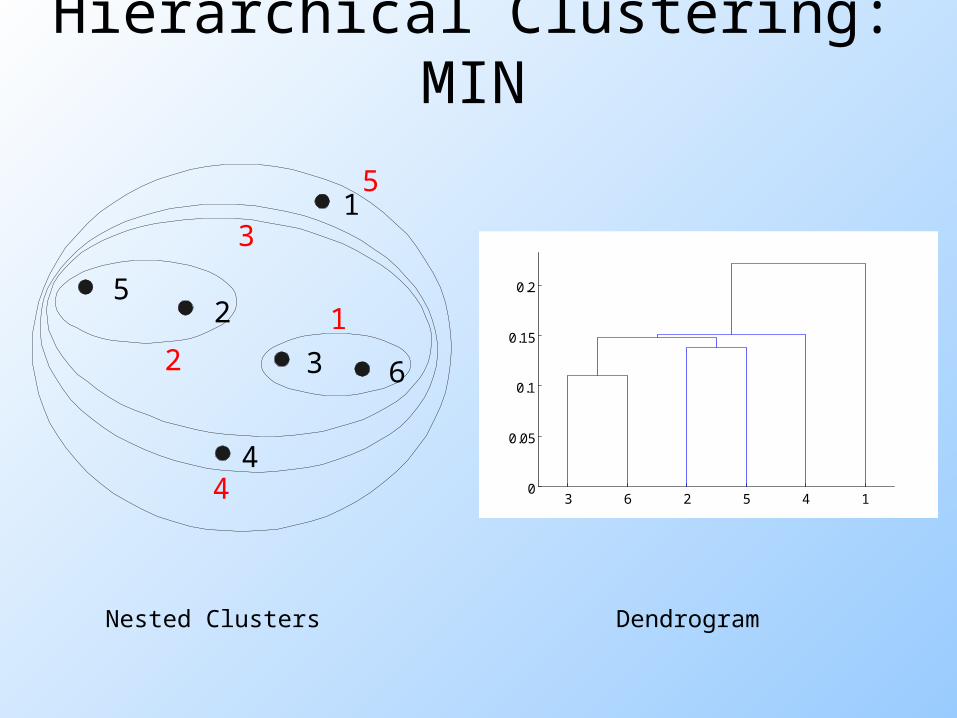
Hierarchical Clustering: MIN
Nested Clusters Dendrogram
1
2
3
4
5
6
12
3
4
5
3 6 2 5 4 10
0.05
0.1
0.15
0.2
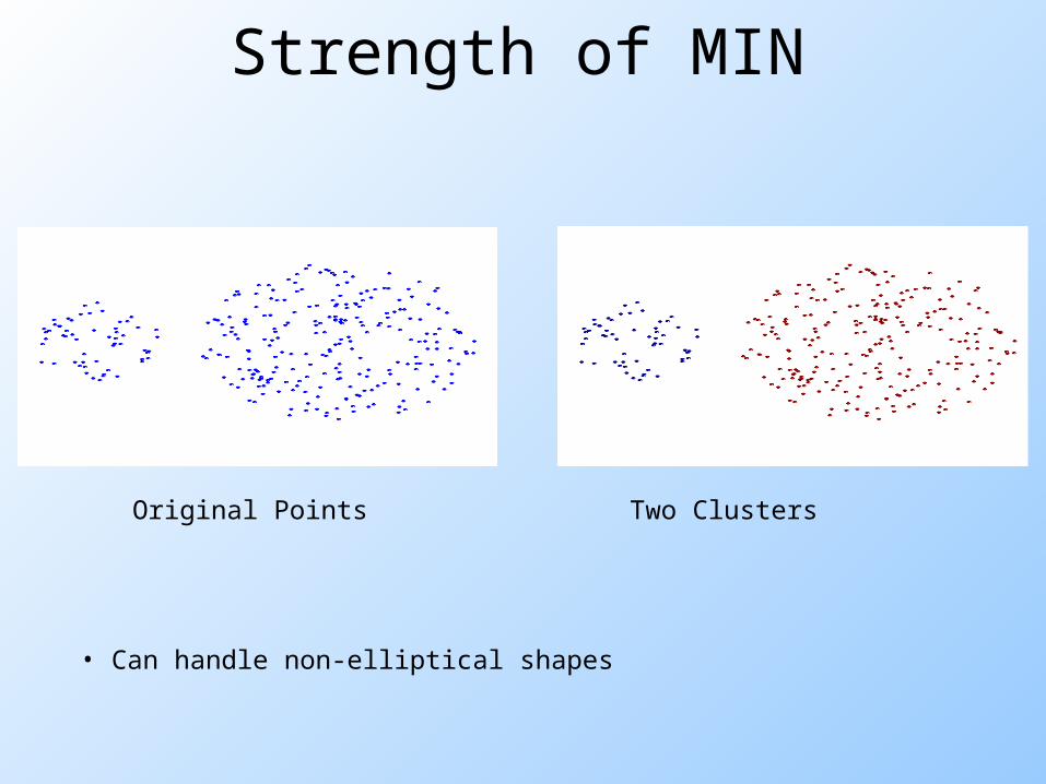
Strength of MIN
Original Points Two Clusters
• Can handle non-elliptical shapes
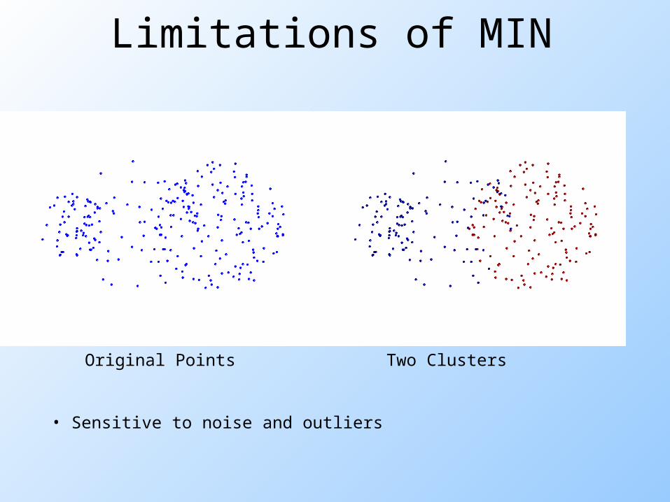
Limitations of MIN
Original Points Two Clusters
• Sensitive to noise and outliers
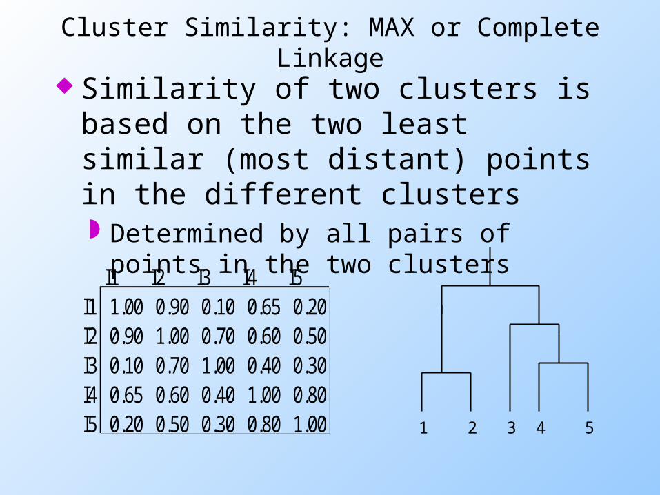
Cluster Similarity: MAX or Complete Linkage
Similarity of two clusters is based on the two least similar (most distant) points in the different clusters Determined by all pairs of points in
the two clustersI1 I2 I3 I4 I5I1 1.00 0.90 0.10 0.65 0.20I2 0.90 1.00 0.70 0.60 0.50I3 0.10 0.70 1.00 0.40 0.30I4 0.65 0.60 0.40 1.00 0.80I5 0.20 0.50 0.30 0.80 1.00 1 2 3 4 5
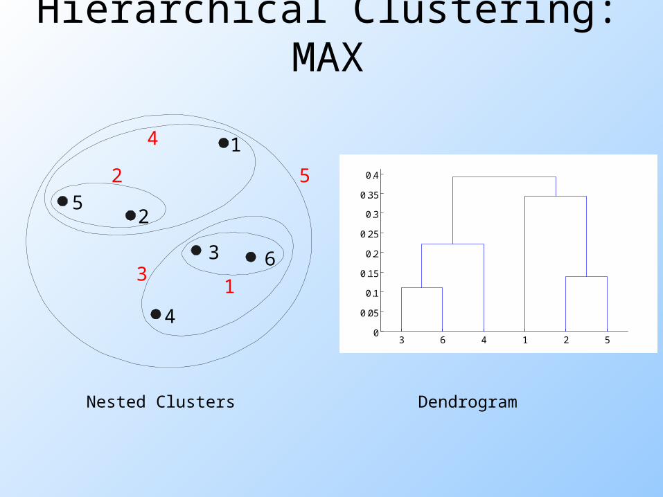
Hierarchical Clustering: MAX
Nested Clusters Dendrogram
3 6 4 1 2 50
0.05
0.1
0.15
0.2
0.25
0.3
0.35
0.4
1
2
3
4
5
6
1
2 5
3
4
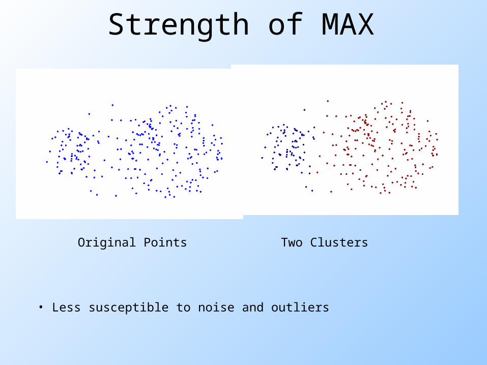
Strength of MAX
Original Points Two Clusters
• Less susceptible to noise and outliers

Limitations of MAX
Original Points Two Clusters
•Tends to break large clusters
•Biased towards globular clusters
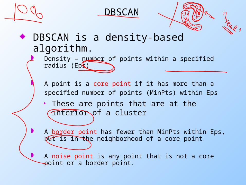
DBSCAN
DBSCAN is a density-based algorithm. Density = number of points within a specified radius
(Eps)
A point is a core point if it has more than a specified number of points (MinPts) within Eps • These are points that are at the interior of
a cluster
A border point has fewer than MinPts within Eps, but is in the neighborhood of a core point
A noise point is any point that is not a core point or a border point.
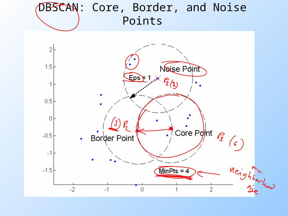
DBSCAN: Core, Border, and Noise Points
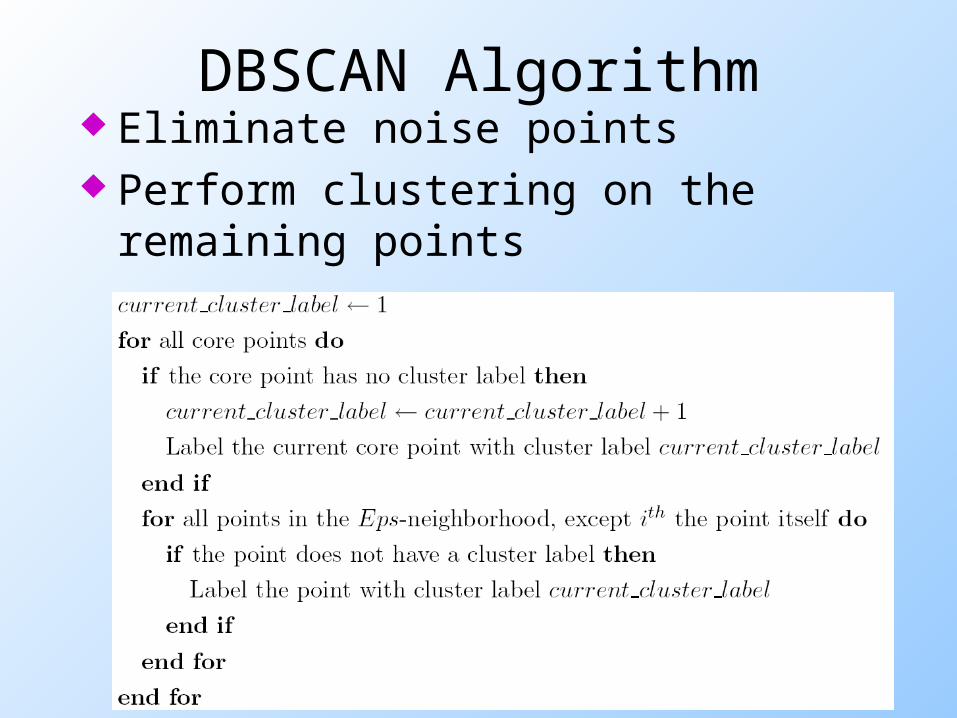
DBSCAN Algorithm Eliminate noise points Perform clustering on the
remaining points
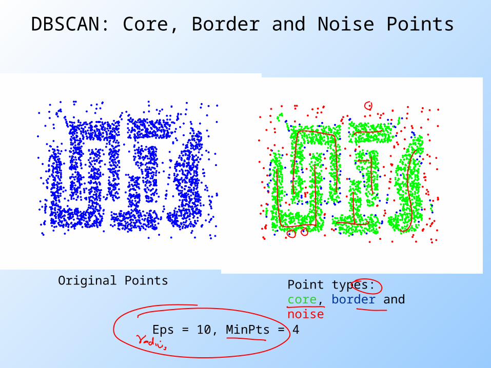
DBSCAN: Core, Border and Noise Points
Original Points Point types: core, border and noise
Eps = 10, MinPts = 4

When DBSCAN Works Well
Original Points Clusters
• Resistant to Noise
• Can handle clusters of different shapes and sizes
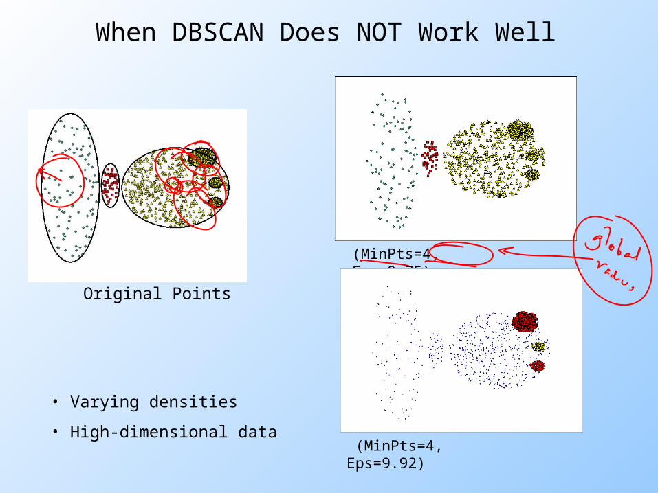
When DBSCAN Does NOT Work Well
Original Points
(MinPts=4, Eps=9.75).
(MinPts=4, Eps=9.92)
• Varying densities
• High-dimensional data
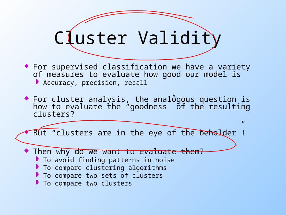
Cluster Validity For supervised classification we have a variety of
measures to evaluate how good our model is Accuracy, precision, recall
For cluster analysis, the analogous question is how to evaluate the “goodness” of the resulting clusters?
But “clusters are in the eye of the beholder”!
Then why do we want to evaluate them? To avoid finding patterns in noise To compare clustering algorithms To compare two sets of clusters To compare two clusters

Data Mining Association Analysis: Basic
Concepts and Algorithms
© Tan,Steinbach, Kumar Introduction to Data Mining
4/18/2004 26
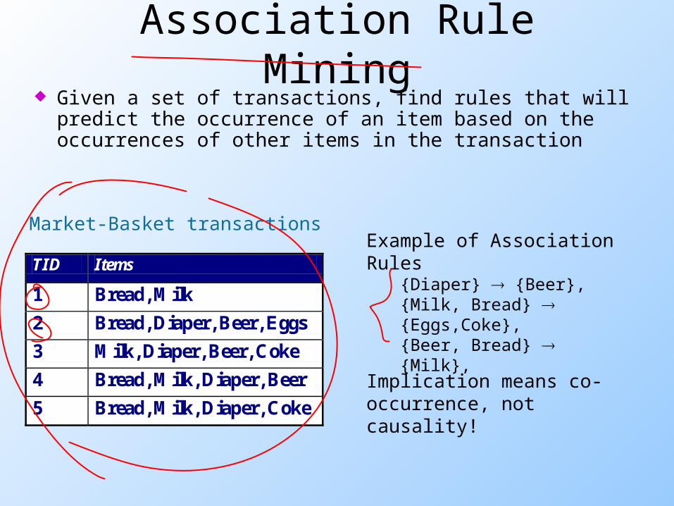
Association Rule Mining Given a set of transactions, find rules that will
predict the occurrence of an item based on the occurrences of other items in the transaction
Market-Basket transactions
TID Items
1 Bread, Milk
2 Bread, Diaper, Beer, Eggs
3 Milk, Diaper, Beer, Coke
4 Bread, Milk, Diaper, Beer
5 Bread, Milk, Diaper, Coke
Example of Association Rules
{Diaper} {Beer},{Milk, Bread} {Eggs,Coke},{Beer, Bread} {Milk},
Implication means co-occurrence, not causality!
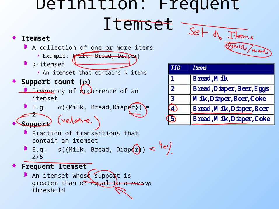
Definition: Frequent Itemset Itemset
A collection of one or more items• Example: {Milk, Bread, Diaper}
k-itemset• An itemset that contains k items
Support count () Frequency of occurrence of an
itemset E.g. ({Milk, Bread,Diaper}) = 2
Support Fraction of transactions that contain
an itemset E.g. s({Milk, Bread, Diaper}) = 2/5
Frequent Itemset An itemset whose support is
greater than or equal to a minsup threshold
TID Items
1 Bread, Milk
2 Bread, Diaper, Beer, Eggs
3 Milk, Diaper, Beer, Coke
4 Bread, Milk, Diaper, Beer
5 Bread, Milk, Diaper, Coke
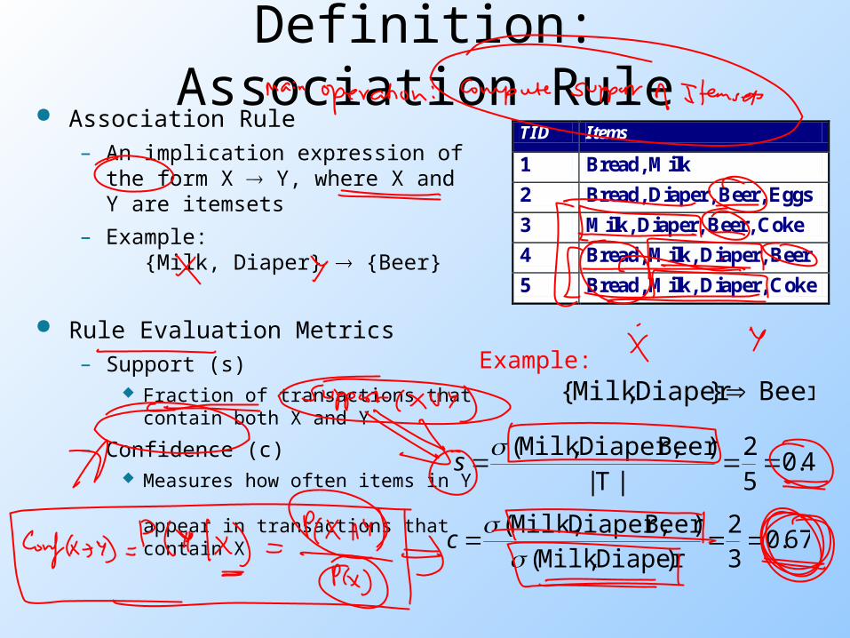
Definition: Association Rule
Example:Beer}Diaper,Milk{
4.052
|T|)BeerDiaper,,Milk(
s
67.032
)Diaper,Milk()BeerDiaper,Milk,(
c
Association Rule– An implication expression of the
form X Y, where X and Y are itemsets
– Example: {Milk, Diaper} {Beer}
Rule Evaluation Metrics– Support (s)
Fraction of transactions that contain both X and Y
– Confidence (c) Measures how often items in Y
appear in transactions thatcontain X
TID Items
1 Bread, Milk
2 Bread, Diaper, Beer, Eggs
3 Milk, Diaper, Beer, Coke
4 Bread, Milk, Diaper, Beer
5 Bread, Milk, Diaper, Coke
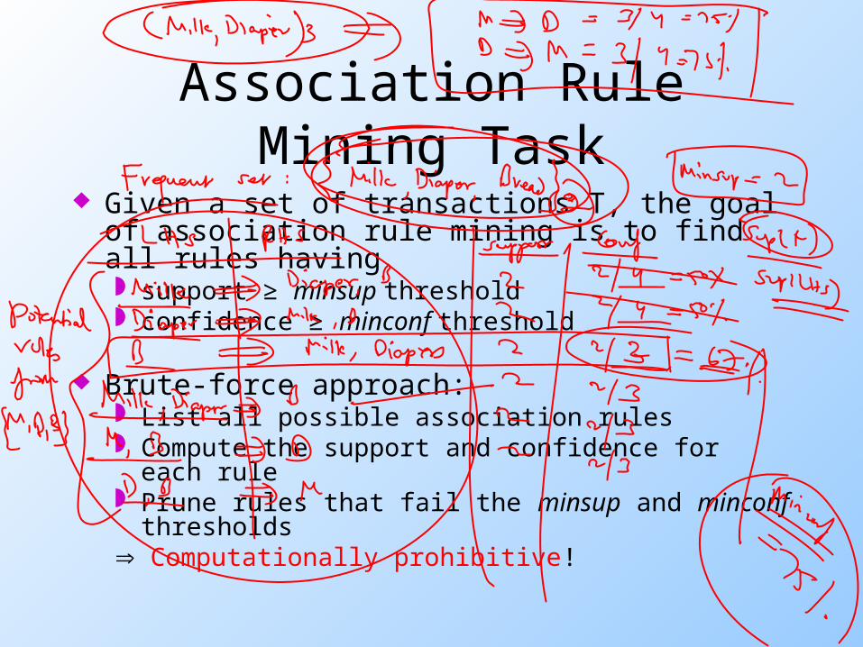
Association Rule Mining Task
Given a set of transactions T, the goal of association rule mining is to find all rules having support ≥ minsup threshold confidence ≥ minconf threshold
Brute-force approach: List all possible association rules Compute the support and confidence for each
rule Prune rules that fail the minsup and minconf
thresholds Computationally prohibitive!
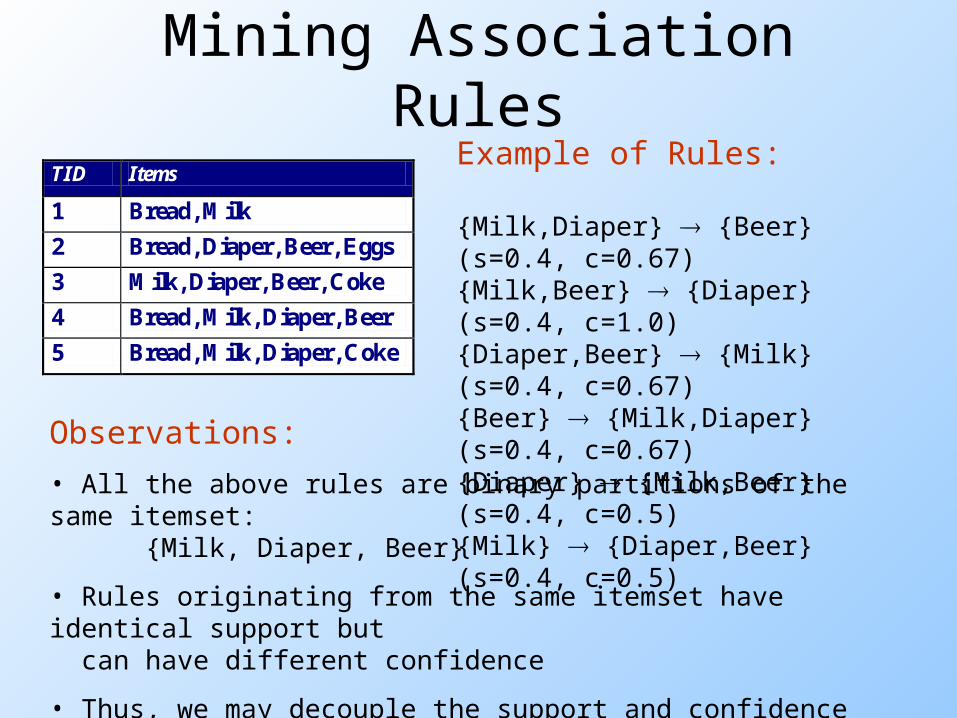
Mining Association RulesExample of Rules:
{Milk,Diaper} {Beer} (s=0.4, c=0.67){Milk,Beer} {Diaper} (s=0.4, c=1.0){Diaper,Beer} {Milk} (s=0.4, c=0.67){Beer} {Milk,Diaper} (s=0.4, c=0.67) {Diaper} {Milk,Beer} (s=0.4, c=0.5) {Milk} {Diaper,Beer} (s=0.4, c=0.5)
TID Items
1 Bread, Milk
2 Bread, Diaper, Beer, Eggs
3 Milk, Diaper, Beer, Coke
4 Bread, Milk, Diaper, Beer
5 Bread, Milk, Diaper, Coke
Observations:
• All the above rules are binary partitions of the same itemset:
{Milk, Diaper, Beer}
• Rules originating from the same itemset have identical support but can have different confidence
• Thus, we may decouple the support and confidence requirements
Mining Association Rules
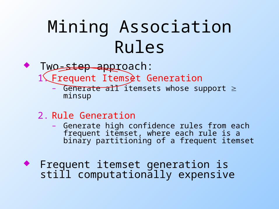
Two-step approach: 1. Frequent Itemset Generation
– Generate all itemsets whose support minsup
2. Rule Generation– Generate high confidence rules from each
frequent itemset, where each rule is a binary partitioning of a frequent itemset
Frequent itemset generation is still computationally expensive
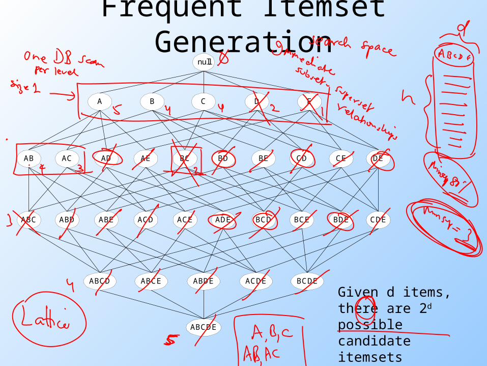
Frequent Itemset Generation
null
AB AC AD AE BC BD BE CD CE DE
A B C D E
ABC ABD ABE ACD ACE ADE BCD BCE BDE CDE
ABCD ABCE ABDE ACDE BCDE
ABCDE
Given d items, there are 2d possible candidate itemsets
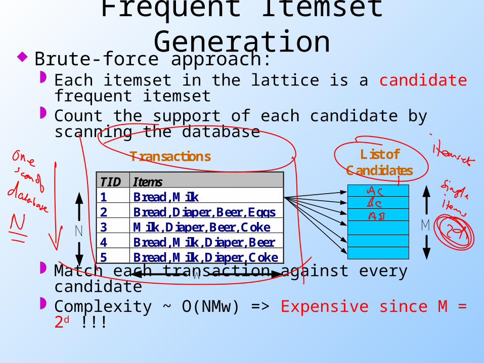
Frequent Itemset Generation Brute-force approach:
Each itemset in the lattice is a candidate frequent itemset
Count the support of each candidate by scanning the database
Match each transaction against every candidate Complexity ~ O(NMw) => Expensive since M =
2d !!!
TID Items 1 Bread, Milk 2 Bread, Diaper, Beer, Eggs 3 Milk, Diaper, Beer, Coke 4 Bread, Milk, Diaper, Beer 5 Bread, Milk, Diaper, Coke
N
Transactions List ofCandidates
M
w
Frequent Itemset Generation Strategies
Reduce the number of candidates (M) Complete search: M=2d
Use pruning techniques to reduce M
Reduce the number of transactions (N) Reduce size of N as the size of itemset
increases Used by DHP and vertical-based mining
algorithms
Reduce the number of comparisons (NM) Use efficient data structures to store the
candidates or transactions No need to match every candidate against
every transaction
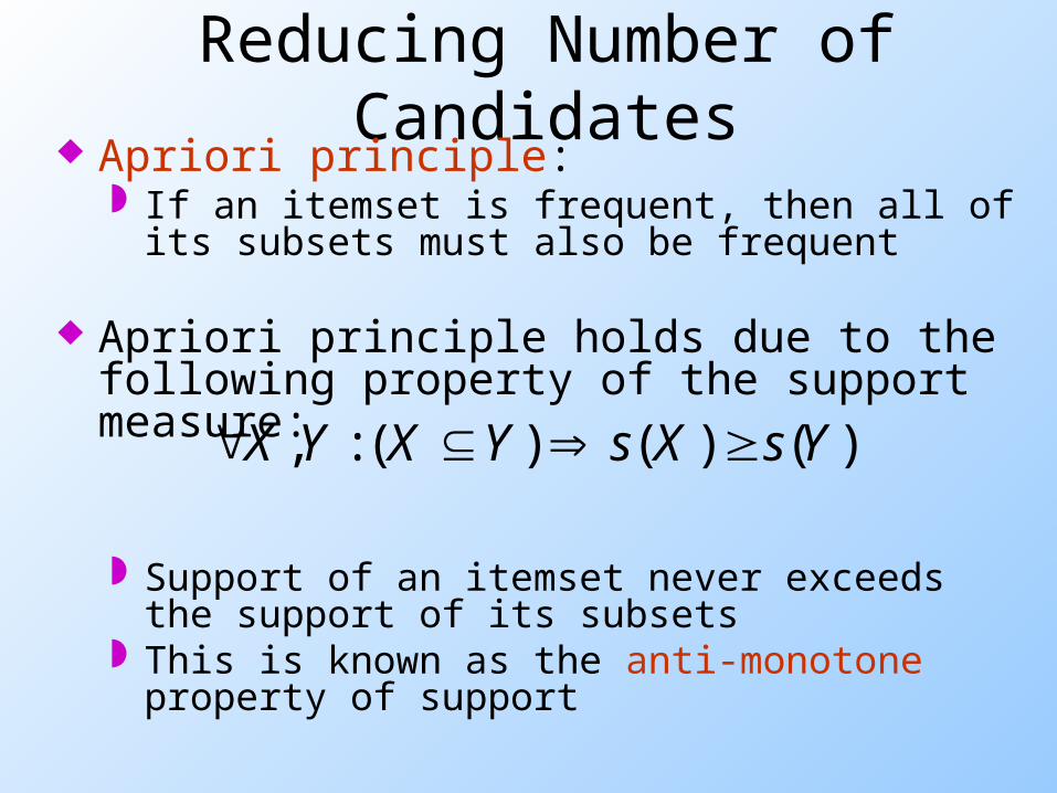
Reducing Number of Candidates Apriori principle:
If an itemset is frequent, then all of its subsets must also be frequent
Apriori principle holds due to the following property of the support measure:
Support of an itemset never exceeds the support of its subsets
This is known as the anti-monotone property of support
)()()(:, YsXsYXYX
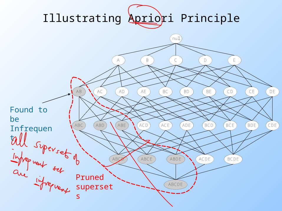
Found to be Infrequent
null
AB AC AD AE BC BD BE CD CE DE
A B C D E
ABC ABD ABE ACD ACE ADE BCD BCE BDE CDE
ABCD ABCE ABDE ACDE BCDE
ABCDE
Illustrating Apriori Principle
null
AB AC AD AE BC BD BE CD CE DE
A B C D E
ABC ABD ABE ACD ACE ADE BCD BCE BDE CDE
ABCD ABCE ABDE ACDE BCDE
ABCDEPruned supersets
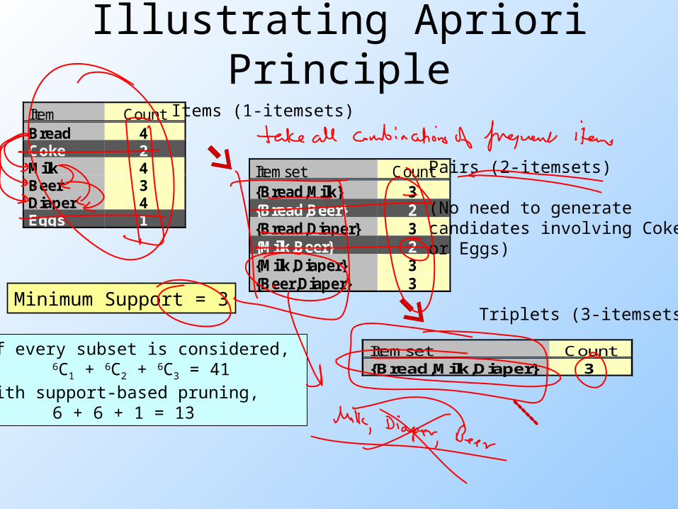
Illustrating Apriori Principle
Item CountBread 4Coke 2Milk 4Beer 3Diaper 4Eggs 1
Itemset Count{Bread,Milk} 3{Bread,Beer} 2{Bread,Diaper} 3{Milk,Beer} 2{Milk,Diaper} 3{Beer,Diaper} 3
Itemset Count {Bread,Milk,Diaper} 3
Items (1-itemsets)
Pairs (2-itemsets)
(No need to generatecandidates involving Cokeor Eggs)
Triplets (3-itemsets)Minimum Support = 3
If every subset is considered, 6C1 + 6C2 + 6C3 = 41
With support-based pruning,6 + 6 + 1 = 13
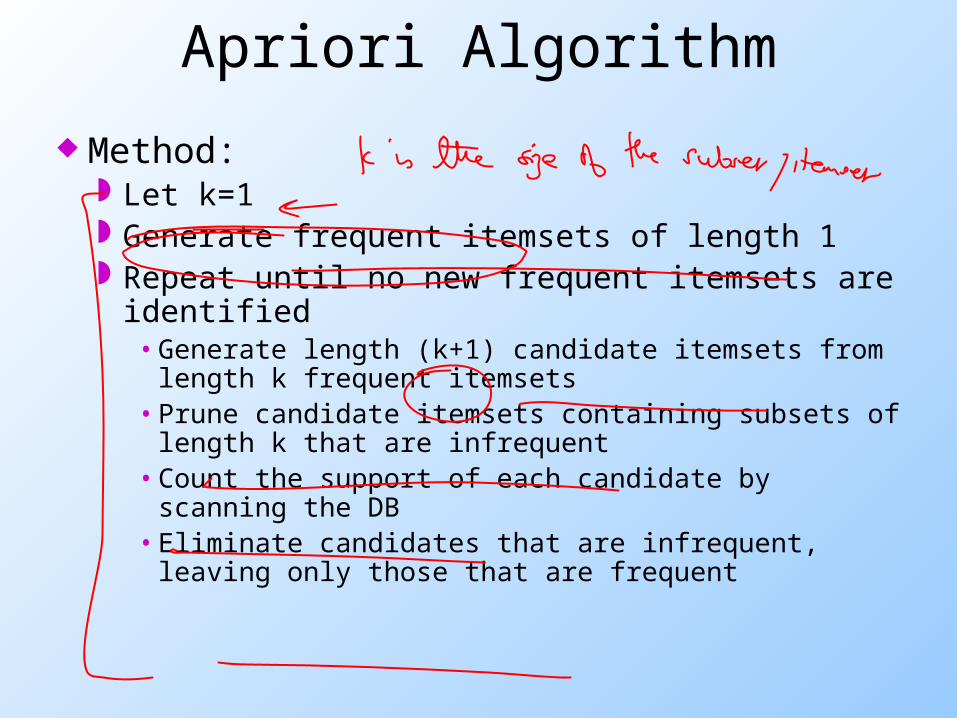
Apriori Algorithm
Method: Let k=1 Generate frequent itemsets of length 1 Repeat until no new frequent itemsets are
identified• Generate length (k+1) candidate itemsets from
length k frequent itemsets• Prune candidate itemsets containing subsets of
length k that are infrequent • Count the support of each candidate by scanning
the DB• Eliminate candidates that are infrequent, leaving
only those that are frequent
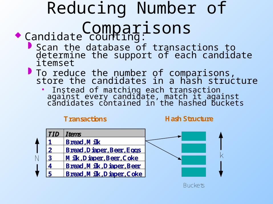
Reducing Number of Comparisons Candidate counting:
Scan the database of transactions to determine the support of each candidate itemset
To reduce the number of comparisons, store the candidates in a hash structure• Instead of matching each transaction against
every candidate, match it against candidates contained in the hashed buckets
TID Items 1 Bread, Milk 2 Bread, Diaper, Beer, Eggs 3 Milk, Diaper, Beer, Coke 4 Bread, Milk, Diaper, Beer 5 Bread, Milk, Diaper, Coke
N
Transactions Hash Structure
k
Buckets
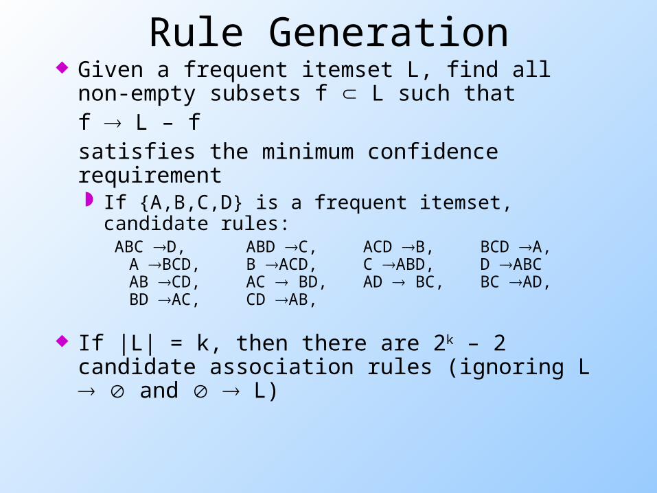
Rule Generation Given a frequent itemset L, find all non-empty
subsets f L such that f L – f satisfies the minimum confidence requirement If {A,B,C,D} is a frequent itemset, candidate rules:
ABC D, ABD C, ACD B, BCD A, A BCD, B ACD, C ABD, D ABCAB CD, AC BD, AD BC, BC AD, BD AC, CD AB,
If |L| = k, then there are 2k – 2 candidate association rules (ignoring L and L)
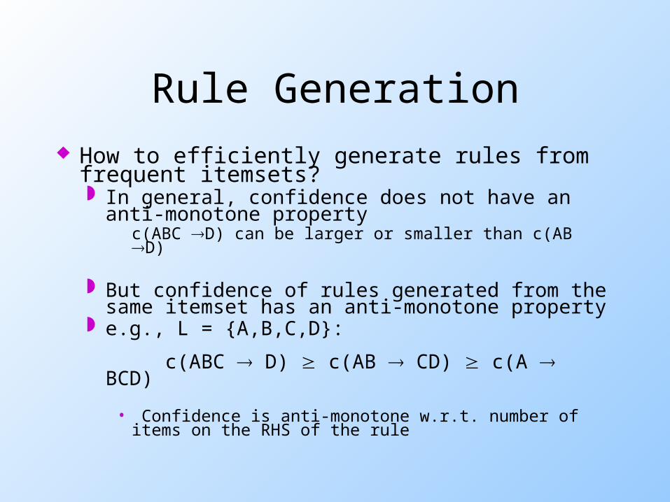
Rule Generation How to efficiently generate rules from
frequent itemsets? In general, confidence does not have an anti-
monotone propertyc(ABC D) can be larger or smaller than c(AB D)
But confidence of rules generated from the same itemset has an anti-monotone property
e.g., L = {A,B,C,D}:
c(ABC D) c(AB CD) c(A BCD)
• Confidence is anti-monotone w.r.t. number of items
on the RHS of the rule
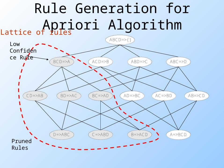
Rule Generation for Apriori Algorithm
ABCD=>{ }
BCD=>A ACD=>B ABD=>C ABC=>D
BC=>ADBD=>ACCD=>AB AD=>BC AC=>BD AB=>CD
D=>ABC C=>ABD B=>ACD A=>BCD
Lattice of rulesABCD=>{ }
BCD=>A ACD=>B ABD=>C ABC=>D
BC=>ADBD=>ACCD=>AB AD=>BC AC=>BD AB=>CD
D=>ABC C=>ABD B=>ACD A=>BCD
Pruned Rules
Low Confidence Rule
Rule Generation for Apriori Algorithm
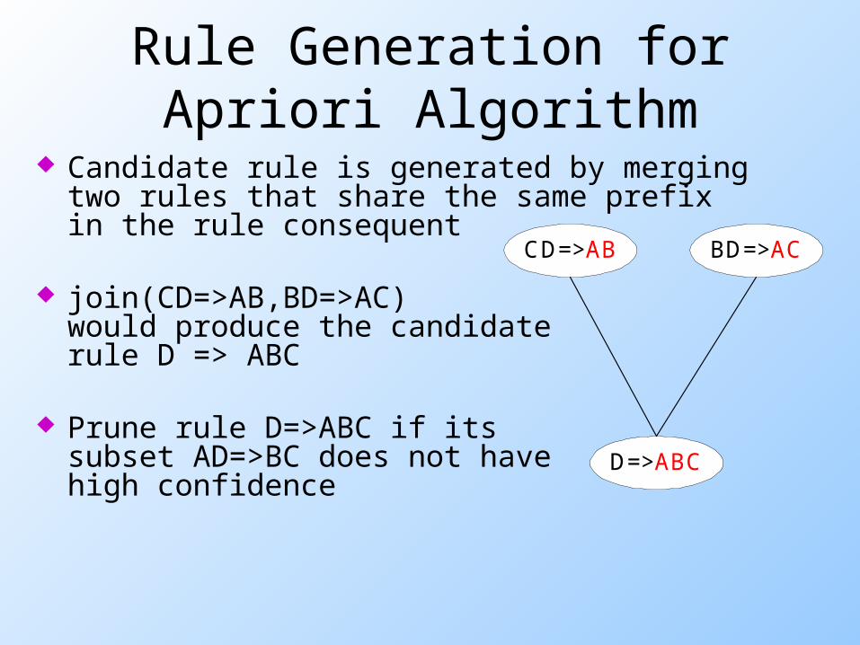
Candidate rule is generated by merging two rules that share the same prefixin the rule consequent
join(CD=>AB,BD=>AC)would produce the candidaterule D => ABC
Prune rule D=>ABC if itssubset AD=>BC does not havehigh confidence
BD=>ACCD=>AB
D=>ABC
Pattern Evaluation
Association rule algorithms tend to produce too many rules many of them are uninteresting or redundant Redundant if {A,B,C} {D} and {A,B} {D}
have same support & confidence Interestingness measures can be used to
prune/rank the derived patterns
In the original formulation of association rules, support & confidence are the only measures used