1

Common Agricultural Policy Regional Impact – The Rural Development Dimension

Collaborative project - Small to medium-scale focused research project under the Seventh Framework Programme

Project No.: 226195

WP3.2 Model development and adaptation – Regional CGEs

Deliverable: D3.2.3

Final documentation of the CGERegEU+ model

DRAFT VERSION

Hannu Törmä, Katarzyna Zawalinska

University of Helsinki, Ruralia Institute

August 31st, 2011

2

Contents

1 Introduction .................................................................................................................................. 3

2 Additions to the base model ......................................................................................................... 3

2.1 Dixon-Parmenter-Sutton-Vincent (DPSV) investment rule .................................................. 3

2.2 Balance of payment equations (EU co-financing of RD measures) ...................................... 6

3 Closures ........................................................................................................................................ 8

3.1 Automatic (technical) closure in Tablo ................................................................................. 8

3.2 Changes to the automatic closure ........................................................................................ 10

3.2.1 Swaps proposed in the closure ..................................................................................... 12

4 Modelling of RD measures ........................................................................................................ 12

4.1 Variables and shocks ........................................................................................................... 13

4.1.1 Modelling investments in human capital ..................................................................... 13

4.1.2 Subsidies for investments in physical capital .............................................................. 14

4.1.3 Direct income transfers ................................................................................................ 15

4.1.4 Land subsidies .............................................................................................................. 15

4.1.5 Subsidies for non-agricultural services in rural areas .................................................. 16

4.2 Parameterization of the shocks ............................................................................................ 16

4.2.1 Shocks for investment in human capital ...................................................................... 16

4.2.2 Shocks for investments in physical capital .................................................................. 16

4.2.3 Shocks for direct income transfers ............................................................................... 17

4.2.4 Shocks for land subsidies ............................................................................................. 17

4.2.5 Shocks for non-agricultural services in rural areas ...................................................... 17

5 Running the base model in GEMPACK .................................................................................... 18

5.1 GEMPACK sub-programs .................................................................................................. 18

5.2 Simulation setup in RunGEM ............................................................................................. 19

6 Conclusions and summary ......................................................................................................... 21

7 List of measures under 2007-2013 RDPs .................................................................................. 22

8 Bibliography............................................................................................................................... 23

3

1 Introduction

This paper documents how to use the CGERegEU model to simulate the Pillar II measures at the

NUTS 2 level for EU27+ countries. It starts with the update on the latest model‟s development after

the deliverable D.3.2.2. The most recent additions concern two aspects: improving the

characteristics of investments (i.e. introducing quasi dynamics in the comparative static model) and

featuring the external co-financing from the EU budget for the Pillar II measures (i.e. adding

balance of payment equations). Further, the paper explains: the possible choices for the model‟s

closures – depending on the policy focus (e.g. short run vs. long run, etc.). It also explains the

simulation design of the RD measures in terms of the variables and shocks implemented. Then it

includes a short manual on how to use the GEMPACK software in order to actually run the model

and produce robust results on the regional impact of Pillar II measures. The paper ends with

summary and conclusions as well as with model coding and electronic version of all essential files

needed to run the model.

2 Additions to the base model

In D3.2.2 we added four new features into the base model. They are: the land factor, different real

wage theories, the Stone-Geary utility function (instead of Cobb-Douglas) and public sector

accounting. Thanks to these additions we have now three primary production factors: labour,

capital, and land. Besides, now we can experiment with different wage theories: sticky wages,

adjusted Phillips curve or Wage curve based real wages. The Cobb-Douglas utility function has

been replaced with the Stone-Geary leading to Linear Expenditure System, which is more

sophisticated. Public sector accounting shows the tax revenues collected, and transfers given.

Comparing to the second deliverable two new features have been added to the model. First, the

investment rule allowing investment demands to be industry specific and endogenous, even if the

model is still comparative static in its nature. Second, balance of payment equations were

introduced to allow taking into account the external EU co-financing of the Pillar II measures from

the EARDF budget.

2.1 Dixon-Parmenter-Sutton-Vincent (DPSV) investment rule

Up till now investments have been exogenous. For our purposes, it is better to use a more advanced

investment rule, which is called DPSV (Dixon, Parmenter, Sutton, and Vincent, 1982, cp. 19).

According to this theory, investments made during a year can affect the capital stock of the same

year. We begin by presenting a conventional investment-capital stock flow mechanism. Small

letters indicate percentage changes.

xcap1 = xinv1 + (1 – δ) xcap0 (all i, r)

xcap0 and xcap1 refer to the capital stock at the beginning and end of the same year, xinv1 is

investment or creation of new capital goods during the year, and δ is the rate of depreciation, wear

4

and tear of the capital stock. The new capital goods xinv1 are assumed to be produced according to

the Leontief structure from domestic inputs.

The only things that affect the capital stock at the end of one year are the current capital stock,

depreciation and investment. It is thus assumed that the effects of past investment decisions are

fully incorporated in the current capital stock.

The theory do not attempt to explain total investments, only how this investment is allocated across

using industries after a change in economic conditions. It is assumed that there is an existing macro

economic policy that determines their size.

The current gross rate of return on fixed capital in a sector, gret is defined as the ratio of the capital

rent, pcap and the cost of a unit of investment, pinv. Net rate of return is received by subtracting the

rate of depreciation of capital.

gret = pcap - pinv (all i,r)

nret = gret - δ

The gross rate of return or profitability will increase (decrease) if the capital rent increases

(decreases) more (less) than investment costs. Increasing profitability implies that the firms are

earning more capital income than they pay as investment costs. We further assume that capital in a

sector takes one year to install.

Investors are assumed to be cautious in assessing the effects of expanding the capital stock in a

sector. They behave as if they expect that sector‟s rate of return schedule in one year‟s time have

the following form.

gret1 = gret0 - β (xcap1 - xcap0)

(all i,r)

0 and 1 represent the situation at the beginning and end of same year, and β is a positive parameter.

The schedule is in the following figure.

5

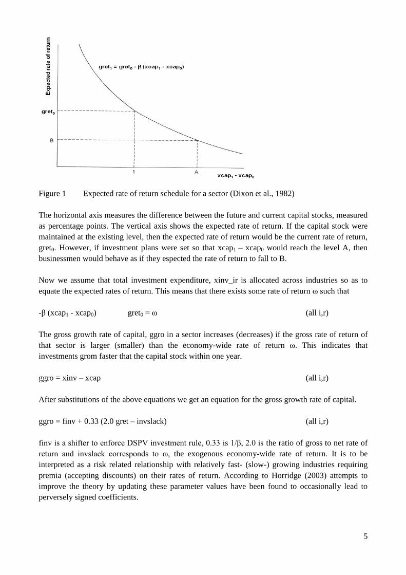
Figure 1 Expected rate of return schedule for a sector (Dixon et al., 1982)

The horizontal axis measures the difference between the future and current capital stocks, measured

as percentage points. The vertical axis shows the expected rate of return. If the capital stock were

maintained at the existing level, then the expected rate of return would be the current rate of return,

gret0. However, if investment plans were set so that xcap1 – xcap0 would reach the level A, then

businessmen would behave as if they espected the rate of return to fall to B.

Now we assume that total investment expenditure, xinv_ir is allocated across industries so as to

equate the expected rates of return. This means that there exists some rate of return ω such that

-β (xcap1 - xcap0) gret0 = ω (all i,r)

The gross growth rate of capital, ggro in a sector increases (decreases) if the gross rate of return of

that sector is larger (smaller) than the economy-wide rate of return ω. This indicates that

investments grom faster that the capital stock within one year.

ggro = xinv – xcap (all i,r)

After substitutions of the above equations we get an equation for the gross growth rate of capital.

ggro = finv + 0.33 (2.0 gret – invslack) (all i,r)

finv is a shifter to enforce DSPV investment rule, 0.33 is 1/β, 2.0 is the ratio of gross to net rate of

return and invslack corresponds to ω, the exogenous economy-wide rate of return. It is to be

interpreted as a risk related relationship with relatively fast- (slow-) growing industries requiring

premia (accepting discounts) on their rates of return. According to Horridge (2003) attempts to

improve the theory by updating these parameter values have been found to occasionally lead to

perversely signed coefficients.

6

Considering the conventional investment-capital stock flow mechanism (see above), total

investment expenditure is as follows.

xinv_ir = ∑i,r pinv xinv (all i,r)

The DPSV rule relates for most sectors the investment of each sector to profitability in that sector.

The effect is that sectors which become more profitable attract more investment. In some sectors,

like in those where investment is determined by government policy, this rule might be

inappropriate. In these sectors investments are not mainly driven by current profits, like in

education, administration etc. For this kind of sectors, it is better to let investment follow aggregate

investment or national/regional trend (Horridge, 2003).

2.2 Balance of payment equations (EU co-financing of RD measures)

Since Pillar II measures are at least partly financed by EU (usually 75% to 80%) we need to take it

into account in our model because the outcomes of the policy differ depending on the source of its

financing (domestic vs. foreign financing). If the policy is fully financed domestically, the spending

has to be covered through savings/earnings obtained elsewhere in the domestic economy (e.g. from

increased government revenues from higher taxes). It is different if the financing comes from

outside of the economy, from abroad (e.g. EU budget1) then it affects the country‟s position vis-a-

vis the rest of the world. Hence it affects the Balance of payments (BOP) accounts, which is a

record of all monetary transactions between a country and the rest of the world.

In the long run, all components of the BOP accounts must sum to zero with no overall surplus or

deficits because all debts have to be paid. Thus, the current account on one side and the capital and

financial account on the other should balance each other out. When an economy, however, has

positive capital and financial accounts (a net financial inflow), the country's debits are more than its

credits (due to an increase in liabilities to other economies or a reduction of claims in other

countries). This is usually in parallel with a current account (trade) deficit; an inflow of money

means that the return on an investment is a debit on the current account. Thus, the economy is using

world savings to meet its local investment and consumption demands. It is a net debtor to the rest of

the world. This is the case of co-financing of RD measures, where the contributions from the

European Agricultural Fund for Rural Development (EAFRD) are counted as capital inflows. That

is why we allow in the model the balance of trade (BOT) moving towards the deficit by the value of

the EAFRD contributions to Pillar II measures, in order to counterbalance BOP.

The following variables and equations were added to the model in order to take account of the BOP

balancing:

1 Of course it has not to be forgotten that countries pay contributions to the EU budget anyway, and some are net

creditors while other are net debtors towards the CAP policy in general.

7

Balance of trade is the difference between the value of total exports and imports to/from the rest of

the world (ROW).

BOT = ∑r VROWEXPtot - ∑r VROWIMPtot

The ratio of the BOT to the value of the expenditure side GDP is of the following form.

R_BOT_GDP = BOT / ∑r GDPEXP

The percentage change in the BOT, d_bot is defined as follows.

100 * d_bot = ∑r VROWEXPtot* (xrowexp_cr + prowexp_cr)

- ∑r VROWIMPtot* (xrowimp_cr + prowimp_cr)

xrowexp_cr and xrowimp_cr are percentage changes of national exports, and prowexp_cr and

prowimp_cr are the corresponding prices. The variables on the parenthes are endogenous, so d_bot

will change according to their adjustment.

The percentage change in the BOT/GDP ratio depends on:

(100 / R_BOT_GDP) * d_bot_gdp = (100 / BOT) * d_bot – wgdpexp_r

Here wgdpexp_r is national nominal expenditure side GDP.

It is important to mention that in case of inflow of euros to the economies which have other than

euro currencies (e.g. zloty in Poland, koruna in Czech Republic, etc.) the inflow makes a pressure

on appreciation of the domestic currencies (prowimp), since euro have to be exchanged into

national currency which increases the demand for it.

Taking into account external co-financing from EARDF requires establishing the following shock

statement in the command file:

Shock d_bot = - x;

where x equals to amount of co-financing from EARDF in mln of national currency. As explained

before, the shock is negative, because percentage change of the balance of trade (d_bot) has to be

put into deficit in order to counterbalance the financial inflows.

8

3 Closures

One important feature of the base model implemented in the GEMPACK software is its ability to

set up closures specific for each policy simulations which can be changed (adjusted) in order to

reflect the reality in the model well as possible. In other words, the choice of closure in CGE model

determines the choice of macroeconomic theory used in simulation and also decides about the

causalities leading to the particular results (Taylor i von Arnim, 2007]. Technically the closure of

the model for a particular simulation specified which variables are exogenous (that is, their values

are given as shocks are unchanged in levels) and which variables are endogenous (that is, the

variable calculated when the model is solved).

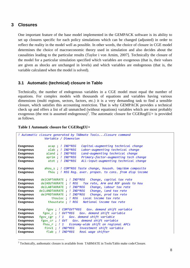
3.1 Automatic (technical) closure in Tablo

Technically, the number of endogenous variables in a CGE model must equal the number of

equations. For complex models with thousands of equations and variables having various

dimensions (multi regions, sectors, factors, etc.) it is a very demanding task to find a sensible

closure, which satisfies this accounting restriction. That is why GEMPACK provides a technical

check up and offers a list of all unmatched (without equations) variables which are most probably

exogenous (the rest is assumed endogenous)2. The automatic closure for CGERegEU+ is provided

as follows.

Table 1 Automatic closure for CGERegEU+

! Automatic closure generated by TABmate Tools...Closure command Variable / Dimension Exogenous acap ; ! IND*REG Capital-augmenting technical change Exogenous alab ; ! IND*REG Labor-augmenting technical change Exogenous aland ; ! IND*REG Land-augmenting technical change Exogenous aprim ; ! IND*REG Primary-factor-augmenting tech change Exogenous atot ; ! IND*REG All-input-augmenting technical change Exogenous ahou_s ; ! COM*REG Taste change, househ. imp/dom composite Exogenous fhou ; ! REG Reg. aver. propen. to cons. from disp income Exogenous delCAPTAXRATE ; ! IND*REG Change, capital tax rate Exogenous delHOUTAXRATE ; ! REG Tax rate, Arm and ROF goods to hou Exogenous delLABTAXRATE ; ! IND*REG Change, labour tax rate Exogenous delLANDTAXRATE ; ! IND*REG Change, land tax rate Exogenous delPRDTAXRATE ; ! IND*REG Change, prod tax rate Exogenous thouloc ; ! REG Local income tax rate Exogenous thoustate ; ! REG National income tax rate Exogenous fgov ; ! COM*GVT*REG Gov. demand shift variable Exogenous fgov_c ; ! GVT*REG Gov. demand shift variable Exogenous fgov_cgr ; ! 1 Gov. demand shift variable Exogenous fgov_cr ; ! GVT Gov. demand shift variable Exogenous fhou_r ; ! 1 Economy-wide shift on regional APCs Exogenous finv1 ; ! IND*REG Investment shift variable Exogenous flab ; ! IND*REG Real wage shifter

2 Technically, authomatic closure is available from TABMATE in Tools/Tablo make code/Closure.

9

Exogenous flab_i ; ! REG Real wage shifter Exogenous flab_ir ; ! 1 Real wage shifter Exogenous flab_r ; ! IND Real wage shifter Exogenous fstatehou ; ! REG Shifter-transf. from nat. gov to reg. hou. Exogenous fstateloc ; ! REG Shifter: transfers from nat. to reg. gov Exogenous fstateloc_r ; ! 1 Shifter: transfers from nat. to reg. gov Exogenous fxserr ; ! COM*REG Xserr shift variable Exogenous invslack ; ! 1 Invest. slack for exogenizing nat. invest Exogenous nhou ; ! REG Number of households Exogenous prowexp ; ! COM Price, exports to ROW, National currency Exogenous prowimp ; ! 1 Price of imports, National currency Exogenous xcap ; ! IND*REG Quantity of capital demanded Exogenous xhoutot ; ! REG Real Spending by households Exogenous xirof ; ! ROF*REG ROF goods used by investment Exogenous xirow ; ! REG ROW goods for investment Exogenous xland ; ! IND*REG Quantity of land (resource) demanded Rest endogenous; ! end of TABmate automatic closure

The first block of the exogenous variables (Table1) covers all technical change variables which are

usually exogenous as in CGERegEU+ (unless the model has built in the endogenous growth theory

in it). There are several input-augmenting technical change variables for individual or grouped

inputs, i.e. labor-augmenting technical change (alab), capital-augmenting technical change (acap),

land-augmenting technical change (aland), and also combined input technical changes, i.e.primary-

factor-augmenting technical change (aprim) and all-input-augmenting technical change (atot). In

case of all technical change variable, the negative shock means that the technology improved in

terms of the particular input, so less of the input is needed to obtain the same amount of output than

before (the whole isoquant shifts).

Apart from technical variables also the taste variable is included (ahou_s) and the propensity to

consume which both are naturally set up outside of the model, at least in the short run closure. The

next block of exogenous variables consists of the tax rates both indirect (on labour, land, capital,

goods and production) and direct (local and national income tax). Since those variables are policy

tools they naturally come as exogenous in the model.

Another exogenous block of variables covers a broad range of shifters. Shift variables are ones that

are originally exogenous and they are used in order to switch on or off certain equations in order to

choose which variant of the theory we want to follow. For example in the labour market block there

is one real wage equation per wage theory, with labour shifters. Three wage theories offer a choice

between sticky wages in the short run vs fully adjustable nominal wages along wage curve (see the

equations explained in D3.2.2). There are real wage shifters (flab shifters) in all real wage theories

with different sectoral and regional dimensions. Consider the first theory. When the shifters are

exogenous their value will be zero. In this case nominal wage follow inflation, so real wage is

sticky. The assumption is the third theory where the change of the unemployment rate and real

wage are determined jointly. In similar fashion work other shifters - in equations for distribution of

government demand, for transfers from government to households, for exogenising national

investment, etc.

10

Further, the number of households is exogenous as well as reference prices (in national currency) -

prowimp - price of imports (numeraire), and prowexp – price of exports. Their exogeneity comes

from the small open economy assumption. Last but not least, the block of certain quantity variables

is exogenous. They include: quantity of capital and land demanded, real spending by households

(from LES), goods used by investment including imported goods to it.

3.2 Changes to the automatic closure

There is no unique or proper closure, on the other hand closure needs to be justifiable. Basically

there are three reasons for which we alter the automatic closure: 1) to take account of the time

horizon of the simulations (short vs. long run closure), 2) to take account of the macroeconomic

features of analysed economies (e.g. small open economy vs. big open economy), 3) to allow

particular policy simulations.

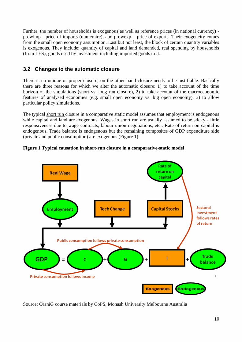
The typical short run closure in a comparative static model assumes that employment is endogenous

while capital and land are exogenous. Wages in short run are usually assumed to be sticky - little

responsiveness due to wage contracts, labour union negotiations, etc.. Rate of return on capital is

endogenous. Trade balance is endogenous but the remaining composites of GDP expenditure side

(private and public consumption) are exogenous (Figure 1).

Figure 1 Typical causation in short-run closure in a comparative-static model

Source: OraniG course materials by CoPS, Monash University Melbourne Australia

11

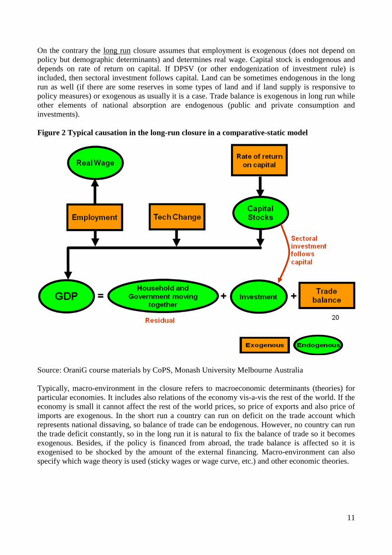
On the contrary the long run closure assumes that employment is exogenous (does not depend on

policy but demographic determinants) and determines real wage. Capital stock is endogenous and

depends on rate of return on capital. If DPSV (or other endogenization of investment rule) is

included, then sectoral investment follows capital. Land can be sometimes endogenous in the long

run as well (if there are some reserves in some types of land and if land supply is responsive to

policy measures) or exogenous as usually it is a case. Trade balance is exogenous in long run while

other elements of national absorption are endogenous (public and private consumption and

investments).

Figure 2 Typical causation in the long-run closure in a comparative-static model

Source: OraniG course materials by CoPS, Monash University Melbourne Australia

Typically, macro-environment in the closure refers to macroeconomic determinants (theories) for

particular economies. It includes also relations of the economy vis-a-vis the rest of the world. If the

economy is small it cannot affect the rest of the world prices, so price of exports and also price of

imports are exogenous. In the short run a country can run on deficit on the trade account which

represents national dissaving, so balance of trade can be endogenous. However, no country can run

the trade deficit constantly, so in the long run it is natural to fix the balance of trade so it becomes

exogenous. Besides, if the policy is financed from abroad, the trade balance is affected so it is

exogenised to be shocked by the amount of the external financing. Macro-environment can also

specify which wage theory is used (sticky wages or wage curve, etc.) and other economic theories.

12

Simulations can specifically require some exogenisation of certain variables to shock them or

endogenisation to see the effect on them. For example in case of direct transfers to households (as in

case of early retirement scheme) they are initially endogenous but since we know the amounts

transferred to them we exogenise them so to shock them and then see the policy effects.

3.2.1 Swaps proposed in the closure

All the changes to the automatic closure are done by swapping the initially exogenous variables

with the presently endogenous ones. The following swaps are proposed for our simulations and as

such are the part of the command file (below the automatic closure):

1) Time horizon swaps

! Long-run factor market closure swap xcap = fgret; ! Capital stock determined endogenously swap finv1 = ggro; ! Investment follows xcap swap flab_ir = xlab_ir; ! Total labour is exog. for demographic reasons

2) Macro-environment swaps

swap fgov = xgov; ! Government budget is fixed so the policy affects only the private sector

swap d_bot = prowimp; !Foreign trade is in balance

3) Policy swaps

swap fhou = whou; !to enable direct income transfer as in the case of early retirement

4 Modelling of RD measures

There are more than 40 measures to be modelled within RDP 2000-2006 and 2007-2013. In order to

handle them for all EU27+ NUTS2 regions we need to group them. In D.3.2.1 we proposed 5 major

categories of policy instruments subdivided into altogether 10 fairly homogeneous groups of

measures which can be simulated together. Instruments in group 1 are subsidies for investments in

human capital so they increase productivity (not only labor productivity but also indirectly other

factors‟ productivity) in either agricultural or other services sector; instruments in group 2 are

subsidies for investments in physical capital in such sectors as construction, agriculture, forestry,

and food processing; group 3 gathers measures implemented in form of direct income transfers for

individual farmers or groups of farmers (such as early retirement or young farmers‟ support under

2000-2006 scheme); group 4 can be called compensatory aids and is granted in form of land

subsidies either in agricultural or forestry sector; group 5 combines measures aiming at increasing

non-agricultural activities and outputs in rural areas, which are mainly materializing in a services

13

sector (e.g. tourism, trade, transport, etc.). So they are basically subsidies for non-agricultural

services in rural areas.

4.1 Variables and shocks

For each group of policy measures there is a different policy design. Please also refer to Table 3 in

deliverable D.3.2.1.

4.1.1 Modelling investments in human capital

Among investments in human capital we distinguish two subgroups of measures, those which

directly aim to improve human capital of farmers (or of agricultural sector) and those which aim to

increase human capital (outside of agriculture) in rural areas.

In the first group, improving human capital in agricultural sector, we would model the following

measures: 111, 114, 115, 132, 133, 142, 143 and 331 (see list of measures in Annex 7.5). They are

mostly related to improving labour productivity of farmers but also other types of productivity

because farmers get more training and information also on how to use other inputs more effectively

and efficiently.

1) The proposed shocks are to total factor productivity in agricultural sector: atot (IND*REG):

all-input-augmenting technical change, where IND would be “AGR” and REG all regions

which have those measures. The value of the shock would be a percentage change between

the TFP in initial situation and TFP after the value of all inputs together are subsidied by the

amount of the measure. This means that thanks to those measures the TFP increased because

the inputs can be saved by the amount of subsidy. So:

,

where Q(i,r) is the initial value of production in agricultural sector in certain region

and I (i,r) is the initial value of all inputs used in agriculture in the region. Then, after

the RDP measures are implemented to improve productivity of human capital in

agricultural sector the total factor productivity it calculated as:

.

The value of the shock is the percentage change difference between the two, so:

*100

Example: If the value of agricultural production in certain region is 100 million and the value of

total factor inputs to agriculture in this region is 80 million, then TFP1 =100/80= 1.25. Then, if the

value of all measures related to human capital for agriculture in this region is let‟s say 20 million

then TFP2=100/(80-20)= 1.67. Then the shock value = (1.25-1.67)/1.67= -0,25. It means that we

increase TFP in agriculture in certain region by 0,25% due to the RDP measures devoted to

improving human capital productivity. See the next section for appropriate shock notation for the

command file.

14

2) The second group of increasing human capital (outside of agriculture) include: 341, 411-

413, 421, 431, 511. They are measures which aim at increasing the amount of human capital

and non-agricultural economy in rural areas. The difference to the first group is that the

former aimed at increasing productivity of human capital, while those measures aim to

increase the amount of human capital in rural areas by developing non-agricultural

activities. That is why we propose to simulate it as a subsidy to capital3 in non-agricultural

sectors, and primarily in services. So the variable proposed to be shocked now is:

delCAPTAXRATE (IND,REG) - which is a subsidy rate for capital in certain sectors in

certain regions (or more precisely capital tax rate change4). IND can be any of 10 remaining

sectors outside of agriculture5 depending on information which sectors are most stressed in

LDSs of particular NUTS2 region. If it is believed to be small shops then IND can be trade

and transport sector (TTR), or if it is tourism one one can set up IND as hotels and

restaurants (HOT) as a proxy. If the value of the measures devoted to the human capital

outside of agriculture (subsidy) in certain region is S (IND, REG) and the value of capital

(depreciation plus operating surplus gross) in the region in this sector is C (IND, REG) then:

, where “-“ means that it is a subsidy.

Example: If the value of all measures related to human capital outside of agriculture in certain

region is 50 million (value of subsidy) and it is directed into a certain sector IND which value of

capital is 500, then the shock value = - 50/500= - 0.1. The same way for all regions in the model.

4.1.2 Subsidies for investments in physical capital

Within the group of subsidies for investments in physical capital we distinguish three subgroups

of measures: 1) those which support physical construction, 2) those which support agriculture and

forestry potential, 3) those which support food processing.

1) Among the measures granted in form of investments in physical capital which support

constructions are: 112, 121, 131, 141, 321-323 (see list of measures in Annex 7.5). The

proposed shock variable is a subsidy for capital in the construction sector, so the shock

variable would be: delCAPTAXRATE (“CNS”, REG). The shock value in that case would

be the value of the RD measures mentioned above related to the value of capital in the

construction sector in each region.

Example: If in a particular region, the value of all measures mentioned above would be 100 million

and the value of capital in the construction sector would be 500 million, then the shock value =

-100/500 = - 0.20. See section 4.2.2.

2) Among the measures which support agricultural potential/capital directly are: 122, 124, 125,

126. So the proposed shock variable is a subsidy for capital in either agricultural sector or

3 Our model has physical and human capital treated together so it is impossible to subsidise only human capital part of

the total capital. 4 In the model‟s code convention subsidies are expressed as taxes with negative signs.

5 As for reminding, the current database for CGERegEU27+ has aggregation to 11 sectors: (Agriculture (AGR),

Forestry (FOR), Other primary production (OPP), Food processing (FOP), Manufacturing (MAN), Energy (ENE),

Construction (CNS), Trade and Transport (TTR), Hotels and Restaurants (HOT), Other services(OSE). Generally the

model can run with any number of sectors.

15

forestry or combination of both, depending on the situation in particular region. So the

proposed shock variable is a subsidy for capital in agriculture and/or forestry, which in

model notation is: delCAPTAXRATE (“AGR”, REG) and delCAPTAXRATE (“FOR”,

REG). The values of the shocks equal to the values of the above RD measures related to

values of Capital in Agriculture and Forestry, respectively.

Example: If for particular region the value of above measures is 80 million and the capital in

agricultural sector is 100 million, then the shock value = -80/100 = -0.8.

3) Last type of measure in this category is subsidising investments in Food processing. Only

one measure falls in the category, i.e. 123. This measure can be parametrisised analogically

to the other two categories, so we can treat is as a subsidy for capital in the food processing

in each region, i.e. delCAPTAXRATE (“FOP”, REG). The value of the shock for each

region will be the value of the measure 123 related to the value of Capital in Food

processing sector, analogically to the previous example.

4.1.3 Direct income transfers

All the measures which are directly paid to the farmers as a sort of income or pension (not as a

reimbursement and not per hectare and without strict obligations on how it can be spent) are treated

as direct transfers. Here we classify two measures 113 (early retirement) and also 112 (support for

young farmers) in the scheme 2000-2006 (in 2007-2013 period the measure was changed into a

simple investment scheme). We would model these measures as an increase in households‟ nominal

income, through variable wfacinc (REG) and the value of the shock will be the value of above

measures related to the value of factor income by regions. One could argue that apart from the

income effect also some productivity effect should be grasped. However, firstly it would require

separate studies to assess whether the productivity effect is present and of which amount. In some

cases the productivity may not occur in short time at all if a farmer transfers his agricultural

activities to his family member (e.g. son) because in fact the land activated stay in the same family

and the management of the farm may also not change in reality.

Example: If for a particular region the households‟ income from labour, land and capital

endowments equals 20 000 millions, and the value of early measures 113 and 112 (2000-2006)

equals 80 million then the shock value = (80/20 000)*100 = 0.4. In order to take account of farmers

households in the region, the shock can be scaled down by taking into account the share of

agricultural household income in total household income in the region.

4.1.4 Land subsidies

There are several measures which are paid per hectare and which are therefore perceived as land

subsidies. We distinguish two groups of such measures, those related primarily to farm land (211-

216, 22-225) and those related to forest land (221, 226). In both cases they will be modelled with

variable related to land subsidies, i.e. delLNDTAXRATE (IND, REG), however in the former case

IND will be AGR while in the latter industry will be FOR, i.e. delLNDTAXRATE (“AGR”, REG)

and delLNDTAXRATE (“FOR”, REG). There seems not to be plans to include forest land into the

NUTS 2 SAMs, but this might change. The value of the shock will be calculated by relating the

value of the measures to the value of land (land rentals) from agricultural and forestry sectors, taken

with negative sign (“-“ indicates subsidy).

16

Example: If the value of measures paid per ha of the farm land in a region is 50 million and the

value of land taxes paid in the region is 400 million then the shock value = -50/400 = -0.125.

4.1.5 Subsidies for non-agricultural services in rural areas

Support for non agricultural economy in rural areas which does not include construction (the latter

are in the category of investment subsidies) include axis 3 measures such as 311, 312, and 313.

They are basically supporting development of certain service sectors (tourism, trade, etc.) and aim

at increasing entrepreneurship in rural areas. Hence, in different regions there can be different types

of services supported, so we would model this as a production subsidy for various sectors:

delPRDTAXRATE (IND, REG). Then if in a certain region those measures support small shop

business then the appropriate parametrization would be via delPRDTAXRATE(“TTR”, REG), if

they support mainly tourism, then the good proxy would be delPRDTAXRATE(“HOT”, REG), etc.

The shock value would be the value of the measures related to the value of production of those

particular sectors in the regional economy taken with negative sign.

Example: if in a certain region the measures 311, 312 went mainly to support opening small shops

and 313 was devoted to support development of tourism, then provided that the value of 311 and

312 was 20 million, value of the trade sector in this region was 400 million, the value of measure

313 was 10 million, and the value of hotels and restaurants sector would be 500 million, then the

first shock value = -20/400 = -0.05 and this would be used to shock variable

delPRDTAXRATE(“TTR”, REG). The second shock value = - 10 /500 = -0.02 would be used to

shock variable delPRDTAXRATE(“HOT”, REG). See more options for parametrisation in the next

session.

4.2 Parameterization of the shocks

4.2.1 Shocks for investment in human capital

Shock atot (“AGR”, REG) = - x ;

where x is calculated for each region as follows: x = (TFP1 – TFP2)/TFP2*100

and the formula for calculating TFPs are as follows: TFP1 = VACT2(AGR,r)/VPRIM1(AGR,r)

and TFP2 = VACT2(“AGR”,REG)/[VPRIM1(“AGR”, REG) – Value of Measures (111, 114, 115,

331, 132, 133 142, 331 in each region)]. VACT and VPRIM are the values of the Armington good

(column sum in SAM) and total factor input to a sector (see D3.2.2, Figure 2).

Shock delCAPTAXrate (“AGR”, REG) = -y; where values for y are calculated for each region as follows y = Value of Measures (341, 411-413,

421, 431, 511) / VCAPPT(AGR,REG). Note that “-“means subsidy, while the same variable with

“+” would mean tax. VCAPPT is the capital cost to the firm.

4.2.2 Shocks for investments in physical capital

Shock delCAPTAXrate (“CNS”, REG) = - z; where values for z are calculated for each region as follows z = Value of Measures (112, 121, 131,

141, 321-323) / VCAPPT(CNS,REG).

17

Shock delCAPTAXrate (“AGR”, REG) = - a; Shock delCAPTAXrate (“FOR”, REG) = - b; where values for z are calculated for each region as follows a = Value of Measures (122, 124, 125,

126) / VCAPPT(AGR,REG) or b= Value of Measures (122, 124, 125, 126) / VCAPPT (FOR, REG).

Shock delCAPTAXrate (“FOP”, REG) = - c; where values for c are calculated for each region as follows c = Value of Measure 123 /

VCAPPT(“FOP”,REG).

4.2.3 Shocks for direct income transfers

swap fhou = wfacinc ! in order to exogenise nominal factor income of households by regions

shock wfacinc (REG) = d;

where values for d are calculated as follows d=Value of measures 113 and 1126 /VFACINC (REG),

where VFACINC is net factor income by region.

4.2.4 Shocks for land subsidies

shock delLNDTAXRATE(“AGR”, REG) = - e;

where: e = Value of measures (211-216, 22-225) / VLANDPT(“AGR”,REG)

shock delLNDTAXRATE(“FOR”, REG) = - f;

where: f = Value of measures (221, 226) / VLANDPT(“FOR”,REG), where VLANDPT is the land

cost to the firm.

4.2.5 Shocks for non-agricultural services in rural areas

shock delPRDTAXRATE (IND, REG) = -g;

where: IND can be any sector except agriculture and forestry, so IND = OPP, FOP, ENE, MAN ,

CNS, TTR, HOT or OSE; g = value of the measures (311,312, 313) / VCOST (IND, REG), where

VCOST is input cost of a sector excluding production taxes.

6 Measure 112 was granted only in the budgetary period 2000-2006 in form of direct income support, in 2007-2013 it

was rather the subsidy in physical investments.

18

5 Running the base model in GEMPACK

5.1 GEMPACK sub-programs

GEMPACK is a general purpose package for CGE models and is not model specific. It is not a

single program, but consists of a group of sub-programs, among which the most important ones are:

ViewHAR - a Windows program for viewing data files (.HAR files)

ViewSOL - a Windows program for viewing solution files (.sl4 files)

WinGEM - provides an environment for carrying out modelling and associated tasks.

RunGEM - provides an environment for carrying out simulations with a fixed model

TABmate - editor for TABLO Input files used for creating and modifying the theory of a model

and also command files (.TAB and .CMF files)

AnalyseGE – a Windows program used for analysing simulation results

RunDynam – Windows interfaces for running recursive dynamic models

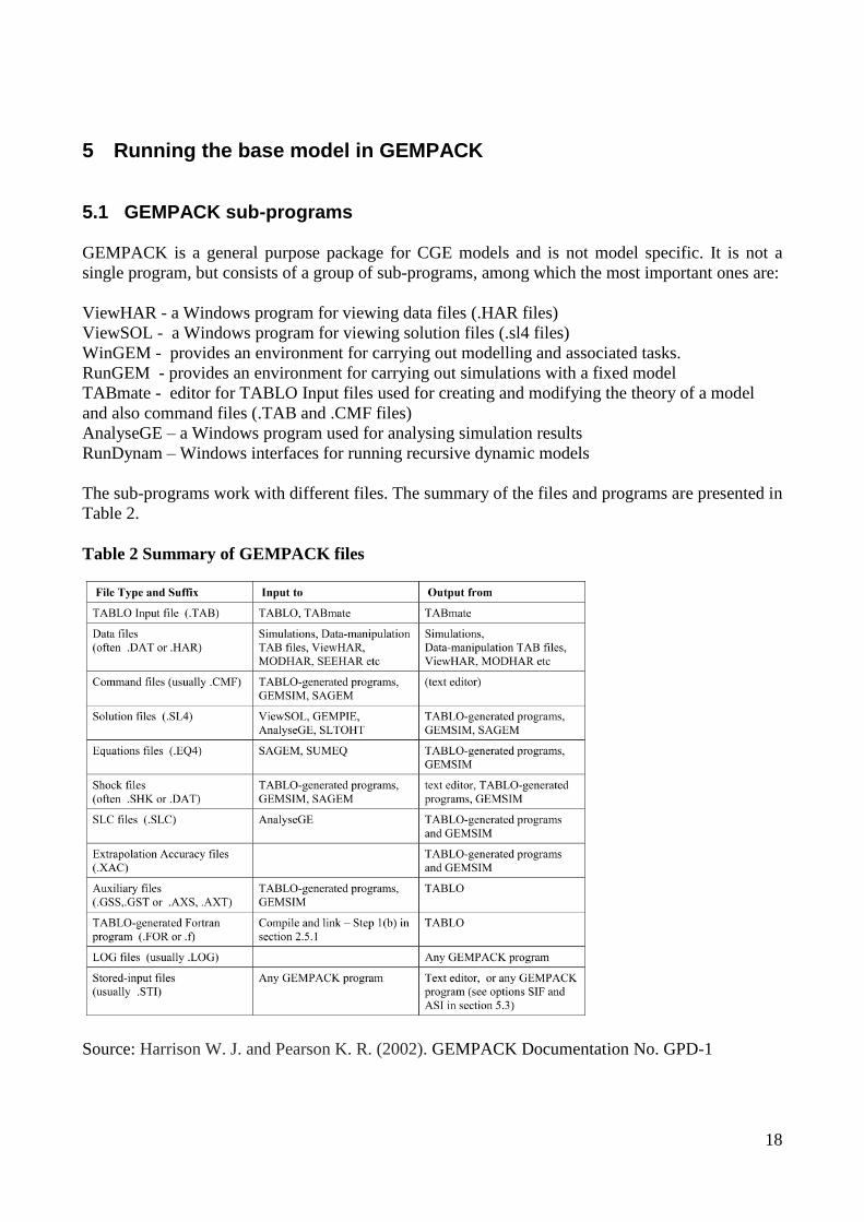
The sub-programs work with different files. The summary of the files and programs are presented in

Table 2.

Table 2 Summary of GEMPACK files

Source: Harrison W. J. and Pearson K. R. (2002). GEMPACK Documentation No. GPD-1

19

5.2 Simulation setup in RunGEM

In order to avoid confusion with use of various GEMPACK sub-programs, we explain how to carry

out simulations with use of only RunGEM. This program leads the user through all the stages of the

simulation process, starting with choice of the model, data, closure, shocks, and then leads to

output, solution and result files as shown in Picture 1.

Picture 1: Simulation process in RunGEM

Source: The RunGEM programme by Monash University

The steps are the following (all required files are included in an email containing also D3.2.3):

1. We choose MODEL which is an .exe file with model (Regfin_for_CAPRI.exe) and the

DATA file (Regfin_for_CAPRI.HAR)

2. Then we choose CLOSURE file (Regfin_for_CAPRI_LR.CLS) which has apart from

automatically generated closure also all amendments to take account of long-run and of our

macro-environment so it has all swaps (described in the previous section) already indicated

but not shocks yet. One can also manually paste the closure in the box offered there by

copying the contents of Table 1 above and swaps from section 3.2.1.

3. The next step is a specification of the SHOCKS. As we described above, for each group of

the policy instruments the shocks are different. The RunGEM programme make the choice

for shock variables easy because in the window “Variable to shock” it offers all variables

which are exogenous at the moment. Besides apart from their short names it offers full

names of selected variables and reminds their dimensions. Then the program prompts you to

select the “Elements to be shocked“, i.e. you can choose sectors (all or particular) or regions

(all or selected ones), etc. Then it asks about the values of shocks. Those have to be

calculated in a separate spreadsheet according to the formulas presented in Section 4.2.

After the specification is ready you click “Add to shock list“. The shock statements can also

20

be copied (as they are presented in section 4.2) and pasted into the box offered there. One

can have prepared shocks for each group of measures as separate files and then only choose

the appropriate file for particular simulation. The programme also reminds the correct

syntax for the shock statement as you proceed.

4. In next step we specify the names of the output (post simulation) files. The following syntax

is an example:

Solution file = “investment subsidies”;

Updated file INFILE = “investment subsidies.upd”;

File SUMMARY= “investment subsidies.ou1”;

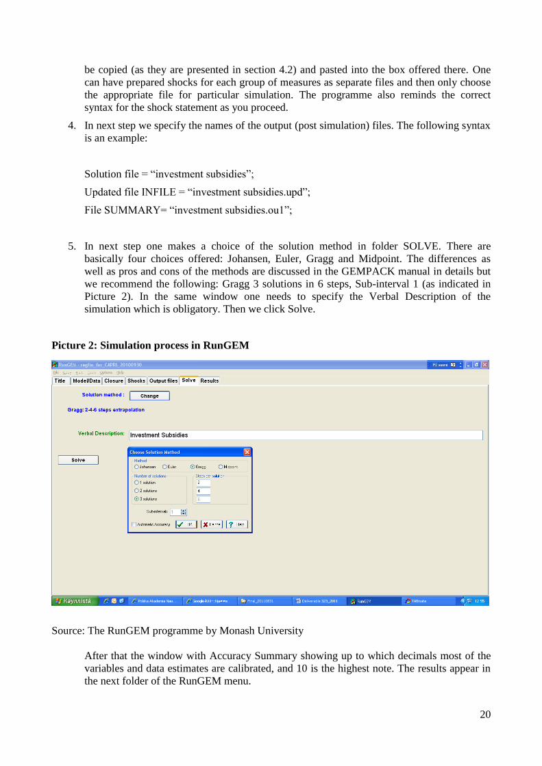
5. In next step one makes a choice of the solution method in folder SOLVE. There are

basically four choices offered: Johansen, Euler, Gragg and Midpoint. The differences as

well as pros and cons of the methods are discussed in the GEMPACK manual in details but

we recommend the following: Gragg 3 solutions in 6 steps, Sub-interval 1 (as indicated in

Picture 2). In the same window one needs to specify the Verbal Description of the

simulation which is obligatory. Then we click Solve.

Picture 2: Simulation process in RunGEM

Source: The RunGEM programme by Monash University

After that the window with Accuracy Summary showing up to which decimals most of the

variables and data estimates are calibrated, and 10 is the highest note. The results appear in

the next folder of the RunGEM menu.

21

6. In the RESULTS folder one can see how individual variables reacted to the shocks

imposed. There is also a group of main variables at the national level to look at first, so

called Macros. There one can see all the variables from the „back of the envelop equations‟.

This makes the interpretation easy, so that it can go from the broader picture of what

happened to the economy down to the regional and sectoral analysis. All the variables in the

solution file are presented as a percentage changes compared to the base year, unless they

are written in capital letters – then they indicate changes in levels.

6 Conclusions and summary

In D3.2.2 and here we have added altogether six new features into the base model. They are: the

land factor, different real wage theories, the Stone-Geary utility function (instead of Cobb-

Douglas), public sector accounting, DPSV investment rule and BOT equations. Thanks to these

additions we have now three primary production factors: labour, capital, and land. Besides, now we

can experiment with different wage theories: sticky wages, adjusted Phillips curve or Wage curve

based real wages. The Cobb-Douglas utility function has been replaced with the Stone-Geary

leading to Linear Expenditure System, which is more sophisticated. Public sector accounting shows

the tax revenues collected, and transfers given. The DPSV investment rule quarantees that

investments within the same year are directed to those sectors that improve their relative

profitability. Finally, the BOT equations make it possible to account for the external EU co-

financing of the Pillar II measures from the EARDF budget.

After introducing the latest two additions to the base model: the DPSV investment rule and the

BOT equations, it also provides a manual type of explanation on how to carry out simulations of the

impact that Rural Development Programs have on the regional economies (NUTS2) in EU27+. In

particular it shows how to use RegCGEEU27+ model in the GEMPACK program in order to model

all rural development measures. The paper suggests the parametrization of the shocks for identified

groups of RD measures, then it explains how to run the simulations.

It is important to mention that there is no one way to model RD measures and there is no widely

agreed consensus on how to do this. Therefore, the proposed simulations have a bit experimental

character. However, they are the best, as to the knowledge of the authors, given the current model

structure of RegGCEEUE27+. At the end of the day, the agricultural economists should decide

about final parameterization, taking note of the structure of the base model.

The obvious challenge is to simulate such complex policy as the CAP (especially Pillar II) at the

regional level. That means that all shocks need to be implemented for c.a. 300 regions. It poses a

challenge not only at the stage of implementation but also for interpretation of the results, where

comparisons of the effect will have to be made with reference to the difference in structure of the

funds obtained by each region within Pillar II.

22

In order to grasp the reality of the simulation we introduced an important feature that allows

specifying to what extent the policy is financed from the national budgets vs. the total EU budget.

This affect the simulation results and bring them more to the reality.

The example how to simulate the policy in RunGEM is not the only option. The simulations can be

run also in WinGEM, but the reason the former was used is that it is precisely designed by CoPS,

Monash University, for running simulations once the model is fixed. The simulation can be built in

a step by step routine which is easy to follow. At the end some general hints are given for

interpretation of the results, however only after true simulations they can be fully explored.

7 List of measures under 2007-2013 RDPs

111 Vocational training and information actions

112 Setting up of young farmers

113 Early retirement

114 Use of advisory services

115 Setting up of management, relief and advisory services

121 Modernisation of agricultural holdings

122 Improvement of the economic value of forests

123 Adding value to agricultural and forestry products

124 Cooperation for development of new products

125 Infrastructure related to agriculture and forestry

126 Restoring agricultural production potential

131 Meeting standards based on Community legislation

132 Participation of farmers in food quality schemes

133 Information and promotion activities for producer groups

141 Semi-subsistence farming

142 Producer groups

143 Direct Payment (Bulgaria + Romania)

211 Natural handicap payments to farmers (mountain areas)

212 Payments to farmers in areas with handicaps (not mountain)

213 Natura 2000 payments and linked to Directive 2000/60/EC

214 Agri-environment payments

215 Animal welfare payments

216 Non-productive investments

221 First afforestation of agricultural land

222 First establishment of agroforestry systems on agri. land

223 First afforestation of non-agricultural land

224 Natura 2000 payments

225 Forest-environment payments

226 Restoring forestry potential and introducing prevention ...

227 Non-productive investments

311 Diversification into non-agricultural activities

312 Business creation and development

23

313 Encouragement of tourism activities

321 Basic services for the economy and rural population

322 Village renewal and development

323 Conservation and upgrading of the rural heritage

331 Training and information

341 Skills acquisition and animation for Local Development Strategies (LDS)

411 Implementing LDS (competitiveness)

412 Implementing LDS (environment/land)

413 Implementing LDS (quality of life/diversification)

421 Implementing cooperation projects

431 Running the local action group, skills acquisition, animation

511 Technical Assistance

8 Bibliography

Böhringer, C., T. F. Rutherford i W. Wiegard (2007). Computable General Equilibrium Analysis

Opening a Black Box. Discussion Paper, Nr 03-56. Mannheim, Centre for European Economic

Research, ZEW.

Borges, A. M. (1986). "Applied General Equilibrium Models: An Assessment of Their Usefulness

for Policy Analysis." OECD Economic Studies 7: 7-43.

Dixon, P. D. and Rimmer M. T. (2002) Dynamic General Equilibrium Modelling for Forecasting

and Policy: A Practical Guide and Documentation of MONASH. North-Holland Amsterdam.

Dixon, P. B., B. R. Parmenter, J. Sutton and D. P. Vincent (1982) ORANI: A Multisectoral Model

of the Australian Economy. Amsterdam: North Holland.

GEMPACK Documentation (2002) by Centre of Policy Studies and Impact Project, Monash

University, Melbourne, Australia

Giesecke, J. A. and Madden J. R. (2003) A large-scale dynamic multi-regional CGE model with an

illustrative application, Review of Urban and Regional Development Studies 15, 2–25.

Harrison W. J. and Pearson K. R. (2002) GEMPACK User Documentation. Centre for Policy

Studies and Impact Project, Monash University, Melbourne Australia.

Honkatukia, J. i R. Vaittinen (2003). POLGEM, A Computable General Equilibrium Model for

Poland. Government Institute for Economic Research, Finland.

Horridge, M. (2003) ORANI-G: A Generic Single-Country Computable General Equilibrium

Model. Centre of Policy Studies, Monash University, http://www.monash.edu.au/

24

policy/oranig.htm.

Horridge, M. and G. Wittwer (2008) Creating and managing an impossibly large CGE database that

is up-to-date. Centre of Policy Studies, Monash University, General Paper No. G-175.

Partridge, M. D. and Rickman D. S. (1998) Regional computable general equilibrium modelling: a

survey and critical appraisal, International Regional Science Review 21, 205–248.

Peter, M. W., Horridge M., Meagher G. A., Naqvi F. and Parmenter B. R. (1996) The Theoretical

Structure of MONASH-MRF . Preliminary Working Paper no. OP-85, IMPACT Project, Monash

University, Clayton, April.

Schwarm W. and Cutler H. (2003) Building small city and town SAMs and CGE models, Review of

Urban and Regional Development Studies 15, 132–147.

Törmä, H. (2008) Do small town development projects matter, and can CGE help? Spatial

Economic Analysis, 3:2, 247–268.

Törmä, H. and Reini K. (2009) Regional Economic Effects of Finnish Mining Sector on Business

Structure and Employment. University of Helsinki, Ruralia Institute. Reports 37.

Törmä, H. and Rutherford T. F. (1993) Integrating Finnish Agriculture into EC‟s Common

Agricultural Policy. Research Report No. 13. Government Institute for Economic Research

Helsinki.

Törmä, H. and Rutherford T. F. (2002) Regional Economic Effects of Building and Using the

Tornio-Kemi Highway, Road Administration of Lappi, printed series (in Finnish, English version

available from www.helsinki.fi/ruralia/research/regfin.htm). (accessed 1 November 2007)

Törmä, H., Rutherford T. F. and Vaittinen R. (1995) What will EU Membership and the Value

Added Tax Reform do to Finnish Food Economy? A Computable General Equilibrium Analysis,

Discussion Paper 88, Helsinki, Government Institute for Economic Research.

Wittwer, G. and Horridge M. (2010) Bringing regional detail to a CGE model using census data,

Spatial Economic Analysis, Volume 5 Issue 2, pp 229-255, Routledge [Jun 3, 2010].