Documentation of the Everglades Landscape Model: … · Documentation of the Everglades Landscape Model: ... 5-29 5.6.4 Periphyton module ... 10.4 Running the model

Documentation of the Everglades Landscape Model:

ELM v2.5 Overview Version of Full Report

http://my.sfwmd.gov/elm

H. Carl Fitz1

Beheen Trimble

South Florida Water Management District 3301 Gun Club Rd

West Palm Beach, FL 33406

1 7512 Model Application Support Unit Hydrologic & Environmental Systems Modeling Dept.

July 10, 2006

ELM v2.5 documentation

ii

Table of Contents Preface.............................................................................................................................vii Executive Summary ......................................................................................................... ix Chapter 1: Introduction, Goals & Objectives ...........................................................1-1

1.1 Overview.......................................................................................................... 1-2 1.2 Introduction...................................................................................................... 1-3 1.3 Purpose of models............................................................................................ 1-6 1.4 ELM goals and objectives................................................................................ 1-7

1.4.1 Objectives, current model version ........................................................... 1-7 1.4.2 Objectives, future model version ............................................................. 1-8

1.5 Literature cited ............................................................................................... 1-10 Chapter 2: Ecological Models: Wetlands..................................................................2-1

2.1 Overview.......................................................................................................... 2-2 2.2 Introduction...................................................................................................... 2-3 2.3 Model Objectives ............................................................................................. 2-3 2.4 Model Design................................................................................................... 2-5

2.4.1 Water........................................................................................................ 2-5 2.4.2 Nutrients................................................................................................... 2-8 2.4.3 Habitat.................................................................................................... 2-11 2.4.4 Animals .................................................................................................. 2-14 2.4.5 Integrated ecosystem.............................................................................. 2-15

2.5 Further Reading ............................................................................................. 2-17 Chapter 3: Conceptual Model...................................................................................3-1

3.1 Overview.......................................................................................................... 3-2 3.2 South Florida Conceptual Model ..................................................................... 3-3

3.2.1 Societal valuation..................................................................................... 3-4 3.2.2 Urban and agricultural development........................................................ 3-5 3.2.3 Water Management.................................................................................. 3-7 3.2.4 Everglades dynamics ............................................................................... 3-9

3.3 General Ecosystem Conceptual Model.......................................................... 3-10 3.3.1 Hydrology .............................................................................................. 3-11 3.3.2 Water Quality......................................................................................... 3-12 3.3.3 Algae/periphyton.................................................................................... 3-13 3.3.4 Macrophytes........................................................................................... 3-14 3.3.5 Soils........................................................................................................ 3-15 3.3.6 Disturbances........................................................................................... 3-16 3.3.7 Animals .................................................................................................. 3-17 3.3.8 Integrated landscape............................................................................... 3-18

Chapter 4: Data ........................................................................................................4-1

4.1 Overview.......................................................................................................... 4-2 4.1.1 Metadata................................................................................................... 4-3

4.2 Model domains................................................................................................. 4-4


iii

4.2.1 Spatial domain ......................................................................................... 4-4 4.2.2 Temporal domain ..................................................................................... 4-5

4.3 Initial condition maps ...................................................................................... 4-5 4.3.1 Water depths ............................................................................................ 4-5 4.3.2 Land surface elevation ............................................................................. 4-6 4.3.3 Soils.......................................................................................................... 4-8 4.3.4 Vegetation .............................................................................................. 4-10

4.4 Static attributes............................................................................................... 4-11 4.4.1 Water management infrastructure.......................................................... 4-11 4.4.2 Model parameters................................................................................... 4-13

4.5 Boundary conditions ...................................................................................... 4-17 4.5.1 Meteorological ....................................................................................... 4-17 4.5.2 Hydrologic ............................................................................................. 4-17 4.5.3 Nutrient/constituent inflows................................................................... 4-19

4.6 Performance assessment targets..................................................................... 4-21 4.6.1 Hydrologic ............................................................................................. 4-21 4.6.2 Water quality.......................................................................................... 4-21 4.6.3 Ecological .............................................................................................. 4-22

4.7 Literature cited ............................................................................................... 4-22 4.8 Tables............................................................................................................. 4-24 4.9 Figure legends................................................................................................ 4-28 4.10 Figures............................................................................................................ 4-29

Chapter 5: Model Structure ......................................................................................5-1

5.1 Overview.......................................................................................................... 5-2 5.1.1 ELM conceptual model............................................................................ 5-3 5.1.2 State variables .......................................................................................... 5-5 5.1.3 Format of algorithm descriptions............................................................. 5-6

5.2 Source code...................................................................................................... 5-7 5.3 Main controller................................................................................................. 5-9 5.4 Data-input modules........................................................................................ 5-10 5.5 Dynamic solutions: sequencing ..................................................................... 5-12 5.6 Vertical solutions ........................................................................................... 5-14

5.6.1 Globals module ...................................................................................... 5-15 5.6.2 Hydrology module ................................................................................. 5-19 5.6.3 Phosphorus, salt/tracer modules............................................................. 5-29 5.6.4 Periphyton module ................................................................................. 5-39 5.6.5 Macrophyte module ............................................................................... 5-48 5.6.6 Floc module ........................................................................................... 5-58 5.6.7 Soils module........................................................................................... 5-64

5.7 Horizontal solutions ....................................................................................... 5-72 5.7.1 Water management: Structure flows module......................................... 5-73 5.7.2 Water management: Canal-marsh flux module ..................................... 5-80 5.7.3 Overland flow module ........................................................................... 5-89 5.7.4 Groundwater flow module ..................................................................... 5-95

5.8 Habitat succession module........................................................................... 5-103 5.9 Literature cited ............................................................................................. 5-105


iv

Chapter 6: Model Performance ................................................................................6-1

6.1 Overview.......................................................................................................... 6-2 6.2 Performance expectations ................................................................................ 6-3

6.2.1 Model application niches ......................................................................... 6-3 6.2.2 ELM v2.5 application niche..................................................................... 6-3 6.2.3 Establishing performance expectations.................................................... 6-3

6.3 Performance evaluation methods..................................................................... 6-5 6.3.1 Calibration process................................................................................... 6-5 6.3.2 Validation process.................................................................................. 6-10 6.3.3 Performance evaluation methods........................................................... 6-11

6.4 Model updates................................................................................................ 6-14 6.5 Model configuration....................................................................................... 6-15 6.6 Performance results........................................................................................ 6-15

6.6.1 Ecological performance ......................................................................... 6-15 6.6.2 Hydrologic performance ........................................................................ 6-29 6.6.3 Ecological consistency........................................................................... 6-45 6.6.4 Validation............................................................................................... 6-48

6.7 Discussion...................................................................................................... 6-51 6.7.1 Model performance summary ................................................................ 6-51 6.7.2 Uncertainty & expectations.................................................................... 6-52 6.7.3 Performance refinements ....................................................................... 6-52 6.7.4 Conclusions............................................................................................ 6-53

6.8 Literature cited ............................................................................................... 6-54 6.9 Appendix A: Computational methods for statistics ....................................... 6-56 6.10 Appendix B: Time series & CFDs: TP (separate pdf) ................................... 6-58 6.11 Appendix C: Time series & CFDs: stage (separate pdf).............................. 6-137 6.12 Appendix D: Water budgets, ELM & SFWMM.......................................... 6-220 6.13 Appendix E: Time series & CFDs: CL (separate pdf) ................................. 6-231

Chapter 7: Uncertainty .............................................................................................7-1

7.1 Overview.......................................................................................................... 7-2 7.2 Data uncertainty ............................................................................................... 7-3

7.2.1 Boundary inflows..................................................................................... 7-3 7.2.2 Tables: data uncertainty ........................................................................... 7-5

7.3 Model sensitivity analyses ............................................................................... 7-6 7.3.1 Sensitivity analysis overview................................................................... 7-6 7.3.2 Model configuration................................................................................. 7-9 7.3.3 Results.................................................................................................... 7-10 7.3.4 Discussion.............................................................................................. 7-11 7.3.5 Tables: sensitivity analyses.................................................................... 7-13 7.3.6 Figures: sensitivity analyses .................................................................. 7-21

7.4 Model complexity .......................................................................................... 7-27 7.4.1 Parameters and complexity .................................................................... 7-27

7.5 Model numerical dispersion........................................................................... 7-29 7.5.1 Figures: dispersion................................................................................. 7-32

7.6 Model “validation”......................................................................................... 7-34


v

7.7 Literature cited ............................................................................................... 7-37 Chapter 8: Model Application ...................................................................................8-1

8.1 Overview.......................................................................................................... 8-2 8.2 Background...................................................................................................... 8-3 8.3 Performance Measure: Phosphorus Accumulation (Net Load) ....................... 8-4

8.3.1 Source of Performance Measure.............................................................. 8-4 8.3.2 Justification.............................................................................................. 8-4 8.3.3 Statistical and Simulation Methods ....................................................... 8-10 8.3.4 Restoration Expectation ......................................................................... 8-12 8.3.5 Projects expected to affect performance measure.................................. 8-14 8.3.6 Evaluation Application .......................................................................... 8-14

8.4 Performance Measure: Phosphorus Concentration........................................ 8-15 8.5 Application Examples.................................................................................... 8-19

8.5.1 Project evaluations ................................................................................. 8-19 8.6 Research applications..................................................................................... 8-26

8.6.1 SFWMD Everglades Division ............................................................... 8-27 8.6.2 Florida Coastal Everglades – LTER ...................................................... 8-27

8.7 Literature Cited .............................................................................................. 8-28 Chapter 9: Model Refinement ..................................................................................9-1

9.1 Overview.......................................................................................................... 9-2 9.2 Version control................................................................................................. 9-2 9.3 Version history................................................................................................. 9-3

9.3.1 ELM beta (1995)...................................................................................... 9-3 9.3.2 ELM v1.0 (1997) ..................................................................................... 9-3 9.3.3 ELM v2.1 (2000) ..................................................................................... 9-3 9.3.4 ELM v2.5 (2006) ..................................................................................... 9-4

9.4 Current limitations ........................................................................................... 9-4 9.5 Planned refinements......................................................................................... 9-5 9.6 Literature cited ................................................................................................. 9-5

Chapter 10: User’s Guide.........................................................................................10-1

10.1 Overview........................................................................................................ 10-2 10.2 Computing environment ................................................................................ 10-3

10.2.1 Hardware................................................................................................ 10-3 10.2.2 Software ................................................................................................. 10-3 10.2.3 Runtimes ................................................................................................ 10-4

10.3 Installing the model........................................................................................ 10-4 10.3.1 Standard ................................................................................................. 10-4 10.3.2 Custom ................................................................................................... 10-4

10.4 Running the model......................................................................................... 10-5 10.4.1 Quick start.............................................................................................. 10-5 10.4.2 Runtime configuration files ................................................................... 10-5 10.4.3 Scripts .................................................................................................... 10-6

10.5 Input data modification .................................................................................. 10-8 10.5.1 Databases ............................................................................................... 10-8


vi

10.5.2 GIS ......................................................................................................... 10-9 10.6 Output .......................................................................................................... 10-10

10.6.1 Quick start............................................................................................ 10-10 10.6.2 Output file structure ............................................................................. 10-10 10.6.3 Debug (errors and warnings) ............................................................... 10-11 10.6.4 Spatial: Basin & Indicator Region (BIR) time series........................... 10-12 10.6.5 Spatial: Domain-wide map time series ................................................ 10-14 10.6.6 Spatial: Point (grid cell) time series..................................................... 10-15 10.6.7 Spatial: Canal (vector) time series ....................................................... 10-16 10.6.8 Spatial: Structure (point/cell) flow time series .................................... 10-16

10.7 Advanced applications ................................................................................. 10-17 10.7.1 Sensitivity analysis............................................................................... 10-17 10.7.2 Evaluating project alternatives............................................................. 10-17 10.7.3 New subregional applications .............................................................. 10-18

10.8 Appendix...................................................................................................... 10-20 10.8.1 Driver.parm configuration file ............................................................. 10-20 10.8.2 Environment variables ......................................................................... 10-23 10.8.3 Directory/file structure......................................................................... 10-23 10.8.4 Software recommendations.................................................................. 10-24


vii

Preface Documentation purpose This documentation report provides the information necessary to fully understand the goals & objectives, supporting data, algorithms, performance, and uncertainties of the Everglades Landscape Model (ELM). This document, the model source code & data, and further supporting information are maintained on the ELM web site:

http://my.sfwmd.gov/elm

Depending on the depth to which one probes, the documentation audience ranges from the lay public to expert scientists:

o The lay-person who is curious about the Everglades and modeling should be able to glean interesting “big picture” insights by reading the Executive Summary, Chapters 1 – 3, and the Overview sections of the remaining Chapters.

o The resource manager who desires a definitive overview of what the ELM can and cannot do will benefit most from the above summaries, along with reviewing sections of Chapters 6 – 8.

o The primary purpose of this documentation, however, is to provide scientists and engineers with hierarchical documentation that a) starts with general overviews which are b) linked to increasing levels of scientific and mathematical detail.

Document organization Each Chapter of this document has its own Table of Contents.

o Chapter 1: Introduction to the Everglades and the model Goals & Objectives.

o Chapter 2: General overview of Wetland Ecological Models.

o Chapter 3: Graphical and verbal descriptions of the South Florida and General Ecosystem Conceptual Models on which the ELM is based.

o Chapter 4: Graphical, verbal, and statistical-summary descriptions all of the Data that are used in the model.

o Chapter 5: Graphical, verbal, and mathematical descriptions of the Model Structure and algorithms (including links to source code).

o Chapter 6: Analysis of Model Performance relative to the historical period of record (1981 - 2000).

o Chapter 7: Aspects of Uncertainty in the model and associated data, including sensitivity analysis, appropriate model expectations, and model complexity.

o Chapter 8: Descriptions of potential Model Applications for research and management.

o Chapter 9: Descriptions of past and planned Model Refinements, including an overview of its current limitations.

o Chapter 10: A User’s Guide that provides the simple steps to installing and running this Open Source model.


viii

Acknowledgments The ELM is the result of long-term collaborative efforts by a diverse group of scientists that extend beyond the current developers. The work was initiated in the early 1990’s by faculty (Robert Costanza, Principal Investigator) at the University of Maryland's Maryland Institute for Ecological Economics, under a contract initiated by Dewey Worth and Tom Fontaine of the South Florida Water Management District (SFWMD). Bob Costanza was the “driver” of the process of understanding the modeling need and how to best meet that need.

The model uses the excellent Spatial Modeling Environment (SME) software developed by the University of Maryland faculty, primarily Tom Maxwell. The University of Maryland’s Alexey Voinov was instrumental in developing numerous vital components of the modeling project, from conceptual models to algorithms and code. Tim Waring and Charles Cornwell made significant contributions while employed at the SFWMD, as did Naiming Wang and Jason Godin. Ken Rutchey aided model development through contributions of vegetation maps and supervision of the ELM team. Also at the SFWMD, Fred Sklar was alternately a Project Manager and a Supervisor during different time periods, and served as a crucial expert in guiding this landscape modeling project.

Beyond anonymous comments received during the publication process of peer reviewed manuscripts, numerous scientists and engineers in south Florida have provided helpful comments on the model and its documentation. Most recently, those reviewers at the SFWMD included Tim Bechtel, Lisa Cannon, Eric Flaig, Tom James, Zaki Moustafa, Garth Redfield, Fred Sklar, Todd Tisdale, Paul Trimble, Dewey Worth, and Joyce Zhang. Comments received during a 2002 Interagency Review of the ELM were likewise useful in improving the model.

Tom Fontaine, Bill Nuttle, Dean Powell, and Patricia Strayer were the senior managers in the SFWMD who supported the ELM project during its primary development phases within the Everglades Systems Research Division. Jayantha Obeysekera, Ken Tarboton, Luis Cadavid, and Ken Konyha managed the project during the recent enhancements to its documentation, leading to the (2006) independent, external peer review of the model and its application.

Primary funding for this modeling project came from the state of Florida through the SFWMD. Funding for the (2006) external peer review of the model came from State and Federal contributions to the Comprehensive Everglades Restoration Plan, and Florida’s Long Term Plan for Achieving Everglades Water Quality Goals.


ix

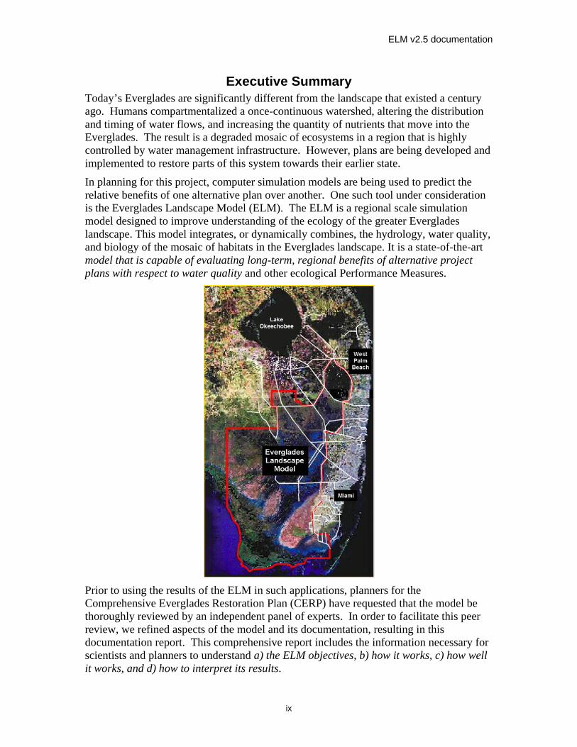
Executive Summary Today’s Everglades are significantly different from the landscape that existed a century ago. Humans compartmentalized a once-continuous watershed, altering the distribution and timing of water flows, and increasing the quantity of nutrients that move into the Everglades. The result is a degraded mosaic of ecosystems in a region that is highly controlled by water management infrastructure. However, plans are being developed and implemented to restore parts of this system towards their earlier state.

In planning for this project, computer simulation models are being used to predict the relative benefits of one alternative plan over another. One such tool under consideration is the Everglades Landscape Model (ELM). The ELM is a regional scale simulation model designed to improve understanding of the ecology of the greater Everglades landscape. This model integrates, or dynamically combines, the hydrology, water quality, and biology of the mosaic of habitats in the Everglades landscape. It is a state-of-the-art model that is capable of evaluating long-term, regional benefits of alternative project plans with respect to water quality and other ecological Performance Measures.

Prior to using the results of the ELM in such applications, planners for the Comprehensive Everglades Restoration Plan (CERP) have requested that the model be thoroughly reviewed by an independent panel of experts. In order to facilitate this peer review, we refined aspects of the model and its documentation, resulting in this documentation report. This comprehensive report includes the information necessary for scientists and planners to understand a) the ELM objectives, b) how it works, c) how well it works, and d) how to interpret its results.


x

Goals • Develop a simulation modeling tool for integrated ecological assessment of water management scenarios for Everglades restoration

o Integrate hydrology, biology, and nutrient cycling in spatially explicit, dynamic simulations

o Synthesize these interacting hydro-ecological processes at scales appropriate for regional assessments,

o Understand and predict the relative responses of the landscape to different water and nutrient management scenarios

o Provide a conceptual and quantitative framework for collaborative field research and other modeling efforts

Application • Specific model objectives (Performance Measures)

o ELM v2.5: Relative predictions of phosphorus 1) concentrations and 2) net load along spatial gradients in the greater Everglades, over decadal time scales

o Other ecological Performance Measures proposed, pending model/data updates • Appropriate applications

o Relative comparisons of the above Performance Measures under scenarios of alternative water management plans

• Project requests for ELM application o CERP: Initial CERP Update, Decompartmentalization of Water Conservation

Area-3, C-111 Spreader Canal, Florida Bay Feasibility Study o Modified Water Deliveries to Everglades National Park (now “CSOP”) o Long Term Plan for Achieving Water Quality Goals: Recovery of Impacted Areas

Design • Encompass the greater Everglades region at fine resolution (10x finer than South

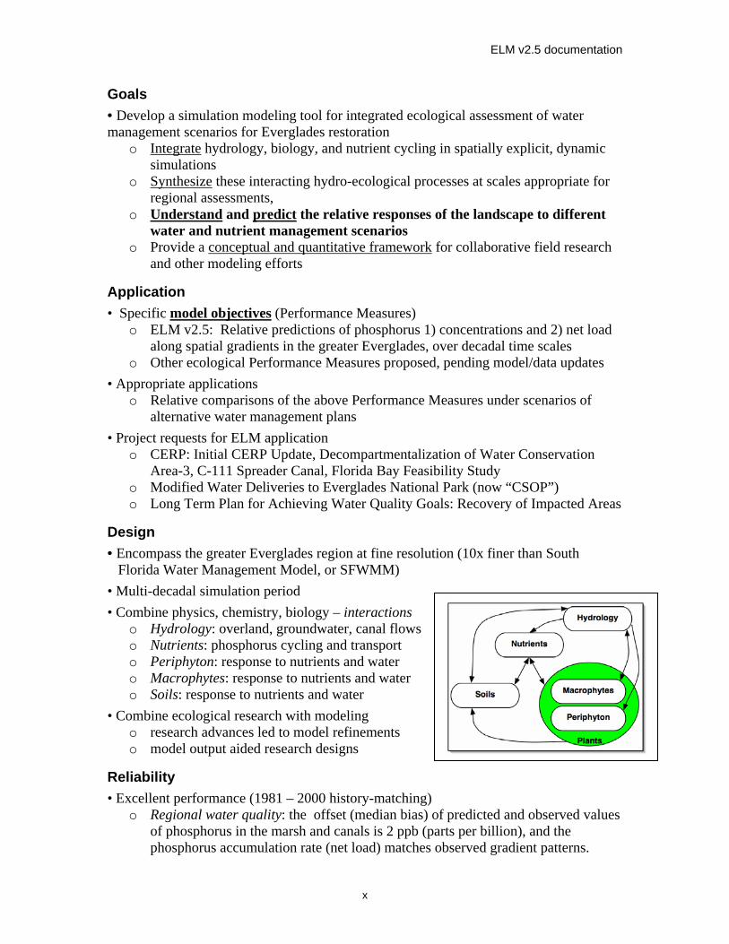
Florida Water Management Model, or SFWMM) • Multi-decadal simulation period • Combine physics, chemistry, biology – interactions

o Hydrology: overland, groundwater, canal flows o Nutrients: phosphorus cycling and transport o Periphyton: response to nutrients and water o Macrophytes: response to nutrients and water o Soils: response to nutrients and water

• Combine ecological research with modeling o research advances led to model refinements o model output aided research designs

Reliability • Excellent performance (1981 – 2000 history-matching)

o Regional water quality: the offset (median bias) of predicted and observed values of phosphorus in the marsh and canals is 2 ppb (parts per billion), and the phosphorus accumulation rate (net load) matches observed gradient patterns.


xi

o Regional hydro-ecology: the ELM hydrologic output is comparable to the SFWMM, and ecological variables such as peat accretion are consistent with available information

• Tested computer code o evaluated model response to wide range of conditions (sensitivity analyses) o years of experience in testing and refining code o applied at different scales for regional and sub-regional evaluations

• Uses best available data o comprehensive, unique summary of Everglades ecology o thorough QA/QC of input data o continuous interactions with other Everglades scientists and engineers

Review • Open Source

o All ELM data and computer source code freely available on web site o Requires only Open Source (free) supporting software

• Publications o 1996-2006: Peer-reviewed scientific journals and book chapters o 1993-2006: Technical reports published by South FL Water Management District

• CERP Model Refinement Team o 2002: Inter-agency review of ELM o 2002: Comments ranged from highly positive to highly negative o 2003: Recommended independent peer review

• Independent Panel of Experts o 2006: July 10, 2006 - Initiated independent peer review of ELM

This page intentionally left blank

ELM v2.5: Chapter Overviews

Overview-1

Overviews of Chapters in ELM Documentation

This document is a greatly abbreviated version of the full documentation report on the Everglades Landscape Model (ELM). (Page numbers in the preceding Table of Contents refer to the full version of the documentation report). The following sections provide a high-level overview of the contents of each Chapter in the full report.

Chapter 1: Introduction, Goals & Objectives Overview

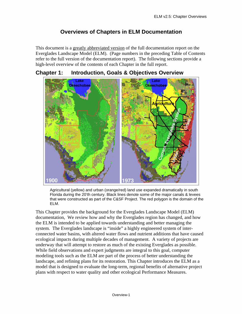
Agricultural (yellow) and urban (orange/red) land use expanded dramatically in south Florida during the 20’th century. Black lines denote some of the major canals & levees that were constructed as part of the C&SF Project. The red polygon is the domain of the ELM.

This Chapter provides the background for the Everglades Landscape Model (ELM) documentation, We review how and why the Everglades region has changed, and how the ELM is intended to be applied towards understanding and better managing the system. The Everglades landscape is “inside” a highly engineered system of inter-connected water basins, with altered water flows and nutrient additions that have caused ecological impacts during multiple decades of management. A variety of projects are underway that will attempt to restore as much of the existing Everglades as possible. While field observations and expert judgments are integral to this goal, computer modeling tools such as the ELM are part of the process of better understanding the landscape, and refining plans for its restoration. This Chapter introduces the ELM as a model that is designed to evaluate the long-term, regional benefits of alternative project plans with respect to water quality and other ecological Performance Measures.


Overview-2

Chapter 2: Ecological Models: Wetlands Overview

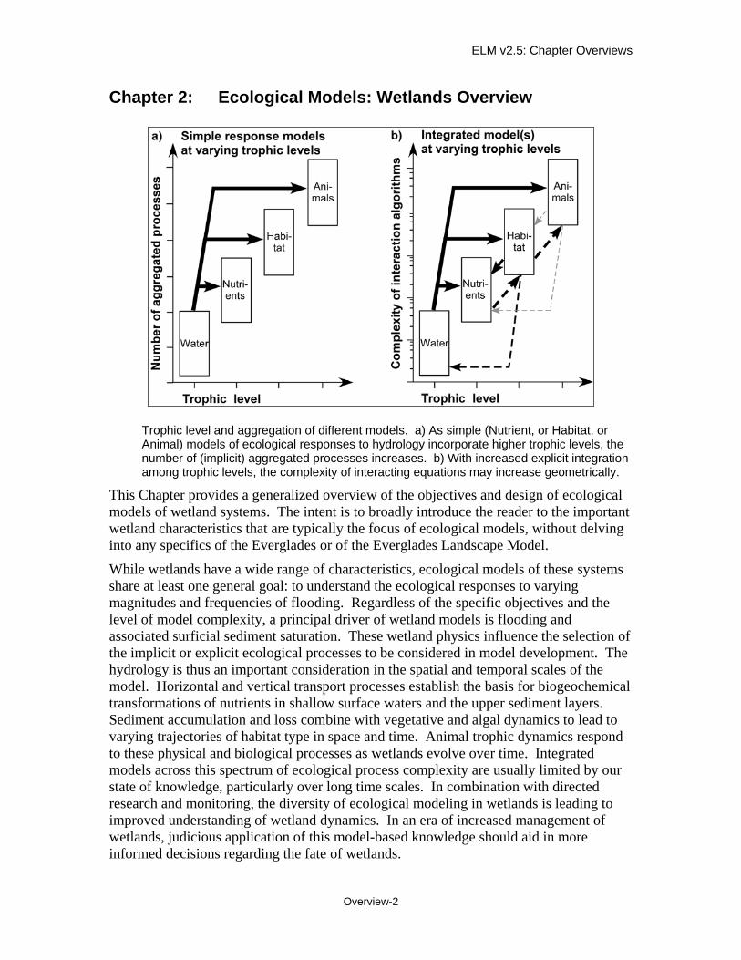
Trophic level and aggregation of different models. a) As simple (Nutrient, or Habitat, or Animal) models of ecological responses to hydrology incorporate higher trophic levels, the number of (implicit) aggregated processes increases. b) With increased explicit integration among trophic levels, the complexity of interacting equations may increase geometrically.

This Chapter provides a generalized overview of the objectives and design of ecological models of wetland systems. The intent is to broadly introduce the reader to the important wetland characteristics that are typically the focus of ecological models, without delving into any specifics of the Everglades or of the Everglades Landscape Model.

While wetlands have a wide range of characteristics, ecological models of these systems share at least one general goal: to understand the ecological responses to varying magnitudes and frequencies of flooding. Regardless of the specific objectives and the level of model complexity, a principal driver of wetland models is flooding and associated surficial sediment saturation. These wetland physics influence the selection of the implicit or explicit ecological processes to be considered in model development. The hydrology is thus an important consideration in the spatial and temporal scales of the model. Horizontal and vertical transport processes establish the basis for biogeochemical transformations of nutrients in shallow surface waters and the upper sediment layers. Sediment accumulation and loss combine with vegetative and algal dynamics to lead to varying trajectories of habitat type in space and time. Animal trophic dynamics respond to these physical and biological processes as wetlands evolve over time. Integrated models across this spectrum of ecological process complexity are usually limited by our state of knowledge, particularly over long time scales. In combination with directed research and monitoring, the diversity of ecological modeling in wetlands is leading to improved understanding of wetland dynamics. In an era of increased management of wetlands, judicious application of this model-based knowledge should aid in more informed decisions regarding the fate of wetlands.


Overview-3

Chapter 3: Conceptual Model Overview

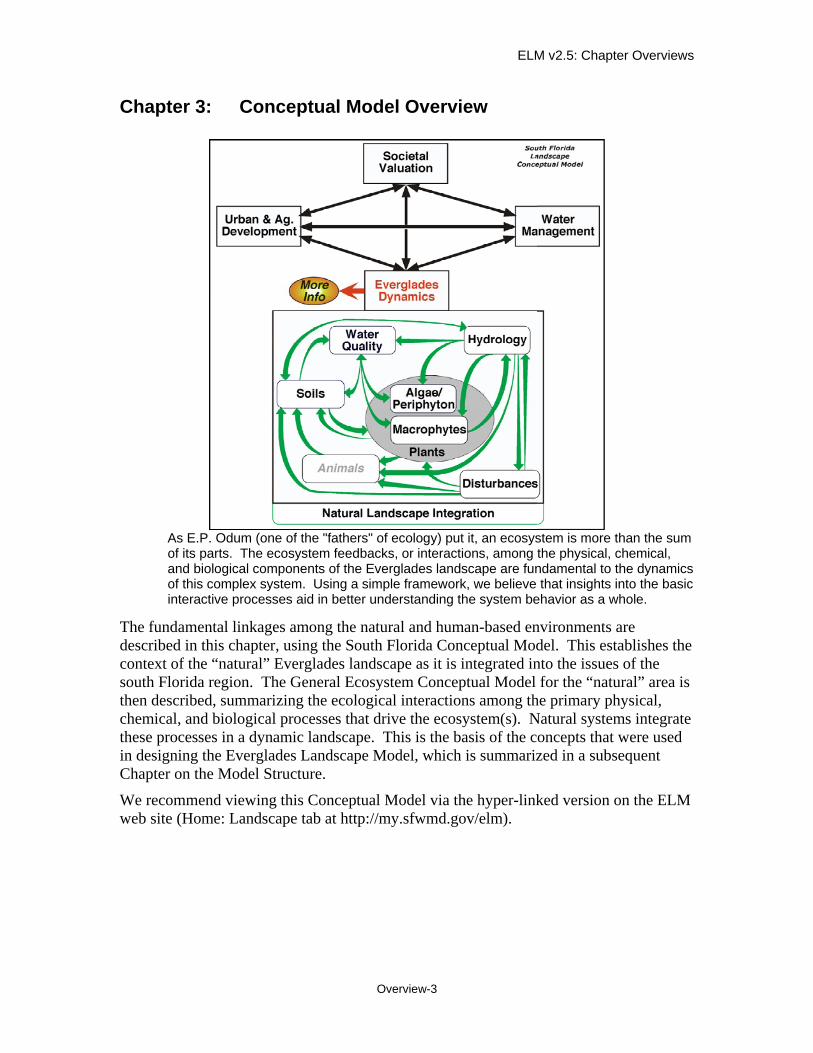
As E.P. Odum (one of the "fathers" of ecology) put it, an ecosystem is more than the sum of its parts. The ecosystem feedbacks, or interactions, among the physical, chemical, and biological components of the Everglades landscape are fundamental to the dynamics of this complex system. Using a simple framework, we believe that insights into the basic interactive processes aid in better understanding the system behavior as a whole.

The fundamental linkages among the natural and human-based environments are described in this chapter, using the South Florida Conceptual Model. This establishes the context of the “natural” Everglades landscape as it is integrated into the issues of the south Florida region. The General Ecosystem Conceptual Model for the “natural” area is then described, summarizing the ecological interactions among the primary physical, chemical, and biological processes that drive the ecosystem(s). Natural systems integrate these processes in a dynamic landscape. This is the basis of the concepts that were used in designing the Everglades Landscape Model, which is summarized in a subsequent Chapter on the Model Structure.

We recommend viewing this Conceptual Model via the hyper-linked version on the ELM web site (Home: Landscape tab at http://my.sfwmd.gov/elm).


Overview-4

Chapter 4: Data Overview

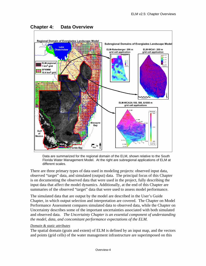
Data are summarized for the regional domain of the ELM, shown relative to the South Florida Water Management Model. At the right are subregional applications of ELM at different scales.

There are three primary types of data used in modeling projects: observed input data, observed “target” data, and simulated (output) data. The principal focus of this Chapter is on documenting the observed data that were used in the project, fully describing the input data that affect the model dynamics. Additionally, at the end of this Chapter are summaries of the observed “target” data that were used to assess model performance.

The simulated data that are output by the model are described in the User’s Guide Chapter, in which output selection and interpretation are covered. The Chapter on Model Performance Assessment compares simulated data to observed data, while the Chapter on Uncertainty describes some of the important uncertainties associated with both simulated and observed data. The Uncertainty Chapter is an essential component of understanding the model, data, and concomitant performance expectations of the ELM. Domain & static attributes The spatial domain (grain and extent) of ELM is defined by an input map, and the vectors and points (grid cells) of the water management infrastructure are superimposed on this


Overview-5

raster map via inputs from two databases. Two other databases contain the model parameters: one documents the parameters that are global across the domain, while the other contains parameters that are specific to the habitats distributed across the domain. Initial conditions These habitats (defined by macrophyte communities) are initialized by an input map, as are other dynamic spatial variables that involve water depths, soil nutrients, land surface elevation, and macrophyte biomass. In the current version, variables such as periphyton biomass and nutrient content are initialized by calculations involving global and/or habitat-specific parameters (i.e., without specific input maps). Boundary conditions The dynamic drivers of the model include spatially explicit, historical time series of rainfall, potential evapotranspiration, stage along the periphery of the domain, water flows through all managed water control structures, and nutrient concentrations associated with inflows into the model domain. Data usage The model was designed to provide the flexibility of modifying the scenario(s) of simulation entirely through Open Source database files, without need to modify the source code of the model. While we necessarily provide details on the derivation of some of the data in this documentation Chapter, the metadata associated with all data sources should impart a sufficient degree of understanding for their usage. An overview of the input methods for these data is provided in the Model Structure Chapter of this documentation, while the User’s Guide Chapter describes the relatively simple steps necessary to run model applications.


Overview-6

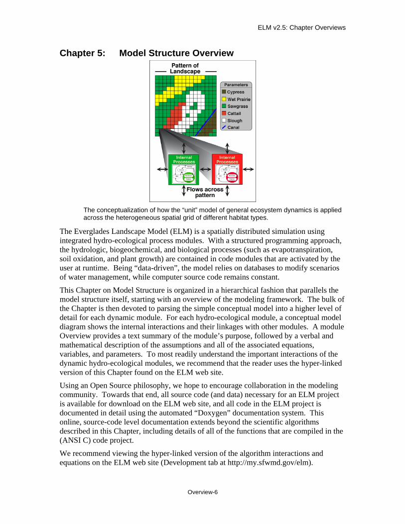
Chapter 5: Model Structure Overview

The conceptualization of how the “unit” model of general ecosystem dynamics is applied across the heterogeneous spatial grid of different habitat types.

The Everglades Landscape Model (ELM) is a spatially distributed simulation using integrated hydro-ecological process modules. With a structured programming approach, the hydrologic, biogeochemical, and biological processes (such as evapotranspiration, soil oxidation, and plant growth) are contained in code modules that are activated by the user at runtime. Being “data-driven”, the model relies on databases to modify scenarios of water management, while computer source code remains constant.

This Chapter on Model Structure is organized in a hierarchical fashion that parallels the model structure itself, starting with an overview of the modeling framework. The bulk of the Chapter is then devoted to parsing the simple conceptual model into a higher level of detail for each dynamic module. For each hydro-ecological module, a conceptual model diagram shows the internal interactions and their linkages with other modules. A module Overview provides a text summary of the module’s purpose, followed by a verbal and mathematical description of the assumptions and all of the associated equations, variables, and parameters. To most readily understand the important interactions of the dynamic hydro-ecological modules, we recommend that the reader uses the hyper-linked version of this Chapter found on the ELM web site.

Using an Open Source philosophy, we hope to encourage collaboration in the modeling community. Towards that end, all source code (and data) necessary for an ELM project is available for download on the ELM web site, and all code in the ELM project is documented in detail using the automated “Doxygen” documentation system. This online, source-code level documentation extends beyond the scientific algorithms described in this Chapter, including details of all of the functions that are compiled in the (ANSI C) code project.

We recommend viewing the hyper-linked version of the algorithm interactions and equations on the ELM web site (Development tab at http://my.sfwmd.gov/elm).


Overview-7

Chapter 6: Model Performance Overview

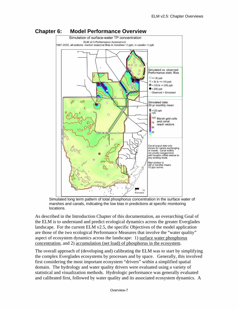
Simulated long term pattern of total phosphorus concentration in the surface water of marshes and canals, indicating the low bias in predictions at specific monitoring locations.

As described in the Introduction Chapter of this documentation, an overarching Goal of the ELM is to understand and predict ecological dynamics across the greater Everglades landscape. For the current ELM v2.5, the specific Objectives of the model application are those of the two ecological Performance Measures that involve the “water quality” aspect of ecosystem dynamics across the landscape: 1) surface water phosphorus concentration, and 2) accumulation (net load) of phosphorus in the ecosystem.

The overall approach of (developing and) calibrating the ELM was to start by simplifying the complex Everglades ecosystems by processes and by space. Generally, this involved first considering the most important ecosystem “drivers” within a simplified spatial domain. The hydrology and water quality drivers were evaluated using a variety of statistical and visualization methods. Hydrologic performance was generally evaluated and calibrated first, followed by water quality and its associated ecosystem dynamics. A


Overview-8

stepwise, hierarchical process followed, evaluating each module of the total system behavior. In this context of the fully integrated ELM, specific aspects of water column phosphorus calibration are required to be associated with reasonable behavior in other ecosystem properties. The best model parameter set becomes that which provides acceptable performance of the primary model application Performance Measures, while maintaining other ecosystem dynamics that are, at minimum, consistent with our best understanding of the Everglades.

In its regional (~10,000 km2) application at 1 km2 grid resolution, the current ELM version 2.5 is available to assess relative differences in ecological performance of Everglades water management plans - at decadal time scales. Hydrologic performance of the ELM is comparable to the South Florida Water Management Model within the Everglades. While consistency with that primary tool for Everglades water management is important, the focus of ELM is on the associated ecological assessment. Extensive data are available for calibrating-validating surface water phosphorus (P) concentrations; during a 2-decade period, the model had a 2 ug L-1 (ppb) median bias in predictions of that Performance Measure within the marshes and canals. Predicted P accumulation along a multiple- decade eutrophication gradient showed a high degree of concordance with P accumulation estimates from radionuclide markers. With other predicted ecological attributes and rates being consistent with available observations, there is cumulative, strong evidence of model skill in predicting phosphorus trends in the regional Everglades landscape at the relevant decadal time scales.


Overview-9

Chapter 7: Uncertainty Overview

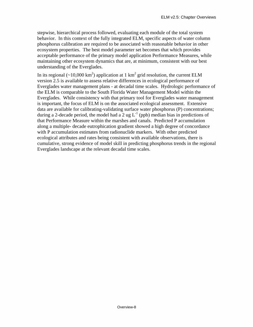
The conceptual model of our approach to analyzing the sensitivity of complex system simulations.

As we noted in the Introduction, Goals & Objectives Chapter, models are simple abstractions of reality, and may be used to guide our thinking. Towards this end, it is vital that modelers and model users acknowledge and understand the uncertainties inherent in any model. The topic of “Uncertainty” is broad, and a thorough treatment of it is well-beyond the scope of this documentation. Instead, we refer the reader to the report of the “Comprehensive Everglades Restoration Plan’s Model Uncertainty Workshop” held in January 2002.

In the Uncertainty Workshop technical report, the authors specifically recommended that the Everglades Landscape Model (ELM) developers repeat the methods of prior sensitivity analyses on the current ELM version. In this chapter, we report on those results, and discuss their implications relative to model complexity.

Hydrology and water quality are primary drivers of the Everglades ecology, and are likewise an important component of the ELM ecological dynamics. Beyond the analysis of model sensitivity to parameter choices, we quantify the statistical expectations of the water quality performance metrics, which are highly dependent on the forces that drive the “boundaries” of the model. Another important concern in water quality modeling is that of “numerical dispersion”, which is explicitly simulated in ELM (see Model Structure Chapter), and discussed here relative to model and data uncertainty.

Finally, we touch upon another common topic in modeling: what is validation, and can modelers truly validate the model output? The basic answer is “No”. However, these model abstractions of reality have served useful purposes in better understanding system dynamics, and will continue to be important tools in aiding our decision-making process for uncertain topics such as understanding and restoring the Everglades.


Overview-10

Chapter 8: Model Application Overview

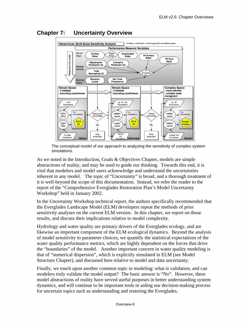
(ELM v2.5.0 output, current version is v2.5.2)

Phosphorus (P) accumulation rates during two scenarios of (10 ppb, and higher historical) phosphorus inflows to the greater Everglades during 1981 - 2000.

The Model Performance chapter of the ELM documentation provides strong evidence of model skill in predicting eutrophication trends across these scales that are of interest in Everglades landscape analysis. In its regional (~10,000 km2) application at 1 km2 grid resolution, the current ELM version 2.5 is available to assess relative differences in ecological performance of Everglades water management plans. Two water quality- oriented model Performance Measures may be used in this interim model version: phosphorus (P) concentration in the surface water, and P accumulation (net load) in the ecosystem. The latter is the more sensitive metric for evaluating ecosystem nutrient status. Consistent with the goals of water management planning for the regional system, the temporal scales of these Performance Measures are multi-decadal with seasonal or annual resolution. Likewise, the spatial scales capture multi-kilometer gradients at a 1-kilometer resolution, within a regional landscape of thousands of square kilometers.

Examples of application of the ELM to scenarios of alternative water management are shown. One example is from recent peer reviewed publication, while the other demonstrates a hypothetical scenario of reduced historical phosphorus inflows. In comparing relative benefits of different alternatives, graphs of trends along gradients and maps of regional differences are presented as examples of model application for planning purposes. Other applications of ELM include the ongoing use of the model in Everglades research programs, wherein the model can help identify information needs. Importantly, models such as ELM can be used to extrapolate and synthesize fine-scaled research results to the larger regional scales of the greater Everglades, across decadal time scales.


Overview-11

Chapter 9: Model Refinement Overview

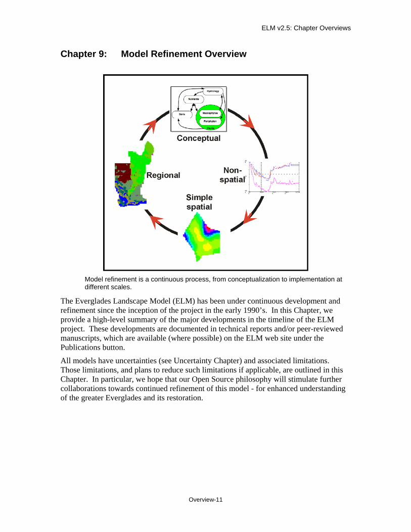
Model refinement is a continuous process, from conceptualization to implementation at different scales.

The Everglades Landscape Model (ELM) has been under continuous development and refinement since the inception of the project in the early 1990’s. In this Chapter, we provide a high-level summary of the major developments in the timeline of the ELM project. These developments are documented in technical reports and/or peer-reviewed manuscripts, which are available (where possible) on the ELM web site under the Publications button.

All models have uncertainties (see Uncertainty Chapter) and associated limitations. Those limitations, and plans to reduce such limitations if applicable, are outlined in this Chapter. In particular, we hope that our Open Source philosophy will stimulate further collaborations towards continued refinement of this model - for enhanced understanding of the greater Everglades and its restoration.


Overview-12

Chapter 10: User’s Guide Overview

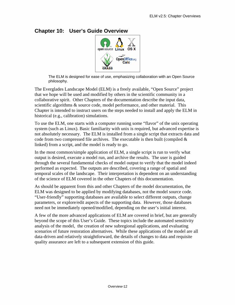
The ELM is designed for ease of use, emphasizing collaboration with an Open Source philosophy.

The Everglades Landscape Model (ELM) is a freely available, “Open Source” project that we hope will be used and modified by others in the scientific community in a collaborative spirit. Other Chapters of the documentation describe the input data, scientific algorithms & source code, model performance, and other material. This Chapter is intended to instruct users on the steps needed to install and apply the ELM in historical (e.g., calibration) simulations.

To use the ELM, one starts with a computer running some “flavor” of the unix operating system (such as Linux). Basic familiarity with unix is required, but advanced expertise is not absolutely necessary. The ELM is installed from a single script that extracts data and code from two compressed file archives. The executable is then built (compiled & linked) from a script, and the model is ready to go.

In the most common/simple application of ELM, a single script is run to verify what output is desired, execute a model run, and archive the results. The user is guided through the several fundamental checks of model output to verify that the model indeed performed as expected. The outputs are described, covering a range of spatial and temporal scales of the landscape. Their interpretation is dependent on an understanding of the science of ELM covered in the other Chapters of this documentation.

As should be apparent from this and other Chapters of the model documentation, the ELM was designed to be applied by modifying databases, not the model source code. “User-friendly” supporting databases are available to select different outputs, change parameters, or explore/edit aspects of the supporting data. However, those databases need not be immediately opened/modified, depending on the user’s initial interest.

A few of the more advanced applications of ELM are covered in brief, but are generally beyond the scope of this User’s Guide. These topics include the automated sensitivity analysis of the model, the creation of new subregional applications, and evaluating scenarios of future restoration alternatives. While these applications of the model are all data-driven and relatively straightforward, the details of changes to data and requisite quality assurance are left to a subsequent extension of this guide.

Documents

Documentation of the Everglades Landscape Model: … · Documentation of the Everglades Landscape Model: ... 5-29 5.6.4 Periphyton module ... 10.4 Running the model