Embed Size (px)
Citation preview
FINAL ASSESSMENT OF THE ECOLOGICAL INTEGRITY OF WOLF CREEK
(LEAVENWORTH COUNTY, KANSAS)
Final report on the investigation of habitat, water quality, and biological conditions in
Wolf Creek
by
Paul Liechti, Principal Investigator
and
Andy Dzialowski, Graduate Research Assistant
Central Plains Center for Bioassessment (CPCB) and
Kansas Biological Survey, University of Kansas, Lawrence, Kansas
December 2003
Disclaimer: This research was funded through EPA 319 funds provided to Leavenworth
County.
Table of Contents
List of Figures.........................................................................................................3
List of Tables..........................................................................................................6
Acknowledgments………………………………………………………………..7
Introduction............................................................................................................8
Watershed Descriptions
Wolf Creek and Reference Streams ……………………………………..9
Data Analysis
Wolf Creek and Reference Streams……..................................………....11
Wolf Creek Results..........................................................……………..................13
Habitat................................................................................…....................13
Water Quality.........................................................................................…21
Periphyton..................................................................................................31
Fish Community....................................................................................….33
Macroinvertebrate Community.............................................................….37
Wolf Creek Conclusions.......................…………….............................................46
Stranger Creek Background ......................……………………........................... 49
Stranger Creek Results
Habitat……………………………………………………………………50
Stranger Creek Conclusions……………………………………………………....55
References...............................................................................................….....…...57
2

List of Figures Figure 1. Map of the Wolf Creek watershed and the sampling sites.............10 Figure 2. Box plots comparing stream shading (%) at Wolf Creek (all three sites combined) and reference streams. Data was also plotted from each Wolf Creek site separately in order to make comparisons between the three sites..………....14 Figure 3. Box plots comparing riparian width (m) of Wolf Creek (all three sites combined) and reference streams. Data was also plotted from each Wolf Creek site separately in order to make comparisons between the three sites.........…......15
Figure 4. Box plots comparing riparian condition of Wolf Creek (all three sites combined) and reference streams. Data was also plotted from each Wolf Creek site separately in order to make comparisons between the three sites. ………....16 Figure 5. Box plots comparing erosion at Wolf Creek (all three sites combined) and reference streams. Data was also plotted from each Wolf Creek site separately in order to make comparisons between the three sites.…….......…...…………………..17
Figure 6. Box plots comparing channel widths at Wolf Creek (all three sites combined) and reference streams. Data was also plotted from each Wolf Creek site separately in order to make comparisons between the three sites……………………..……...…………………………………………… 18
Figure 7. Percent stream bottom cover for inorganic substrate occurring at Wolf Creek (all three sites combined). Data was also plotted from each Wolf Creek site separately in order to make comparisons between the three sites………………………….20 Figure 8. Box plots comparing pH at Wolf Creek (all three sites combined) and reference streams. Data was also plotted from each Wolf Creek site separately in order to make comparisons between the three sites.................................……………….…..22
Figure 9. Box plots comparing turbidity at Wolf Creek (all three sites combined) and reference streams. Data was also plotted from each Wolf Creek site separately in order to make comparisons between the three sites.. ……........……………………...22 Figure 10. Box plots comparing dissolved oxygen (mg/L) at Wolf Creek (all three sites combined) and reference streams. Data was also plotted from each Wolf Creek site separately in order to make comparisons between the three sites......………..23
Figure 11. Box plots comparing conductivity (uohms) at Wolf Creek (all three sites combined) and reference streams. Data was also plotted from each Wolf Creek site separately in order to make comparisons between the three sites......……….25
3
Figure 12. Box plots comparing alkalinity (mg/L) at Wolf Creek (all three sites combined) and reference streams. Data was also plotted from each Wolf Creek site separately in order to make comparisons between the three sites..…...........26 Figure 13. Box plots comparing hardness (mg/L) at Wolf Creek (all three sites combined) and reference streams. Data was also plotted from each Wolf Creek site separately in order to make comparisons between the three sites...………...26 Figure 14. Box plots comparing total nitrogen (mg/L) at Wolf Creek (all three sites combined) and reference streams. Data was also plotted from each Wolf Creek site separately in order to make comparisons between the three sites.....……….27
Figure 15. Box plots comparing total phosphorus (mg/L) at Wolf Creek (all three sites combined) and reference streams. Data was also plotted from each Wolf Creek site separately in order to make comparisons between the three sites.... ……….28 Figure 16. Box plots comparing chemical oxygen demand (mg/L) at Wolf Creek (all three sites combined) and reference streams. Data was also plotted from each Wolf Creek site separately in order to make comparisons between the three sites............................................................................................................…..29
Figure 17. Box plots comparing atrazine (ug/L) at Wolf Creek (all three sites combined) and reference streams. Data was also plotted from each Wolf Creek site separately in order to make comparisons between the three sites...30
Figure 18. Box plots comparing fecal coliform bacteria (org./100 mL) at Wolf Creek (all three sites combined) and reference streams. Data was also plotted from each Wolf Creek site separately in order to make comparisons between the three sites...................................................................................................................31 Figure 19. Box plots comparing chlorophyll a (ug/L) concentrations from the three Wolf Creek sites and Stranger Creek.............................................……......………...33
Figure 20. Box plots comparing average fish species richness for Wolf Creek (all three sites combined) and reference streams. Data was also plotted from each Wolf Creek site separately in order to make comparisons between the three sites……………………………..………......................................................…36 Figure 21. Box plots comparing average fish abundance (inds./m) for Wolf Creek (all three sites combined) and reference streams….................................…...... 36
4
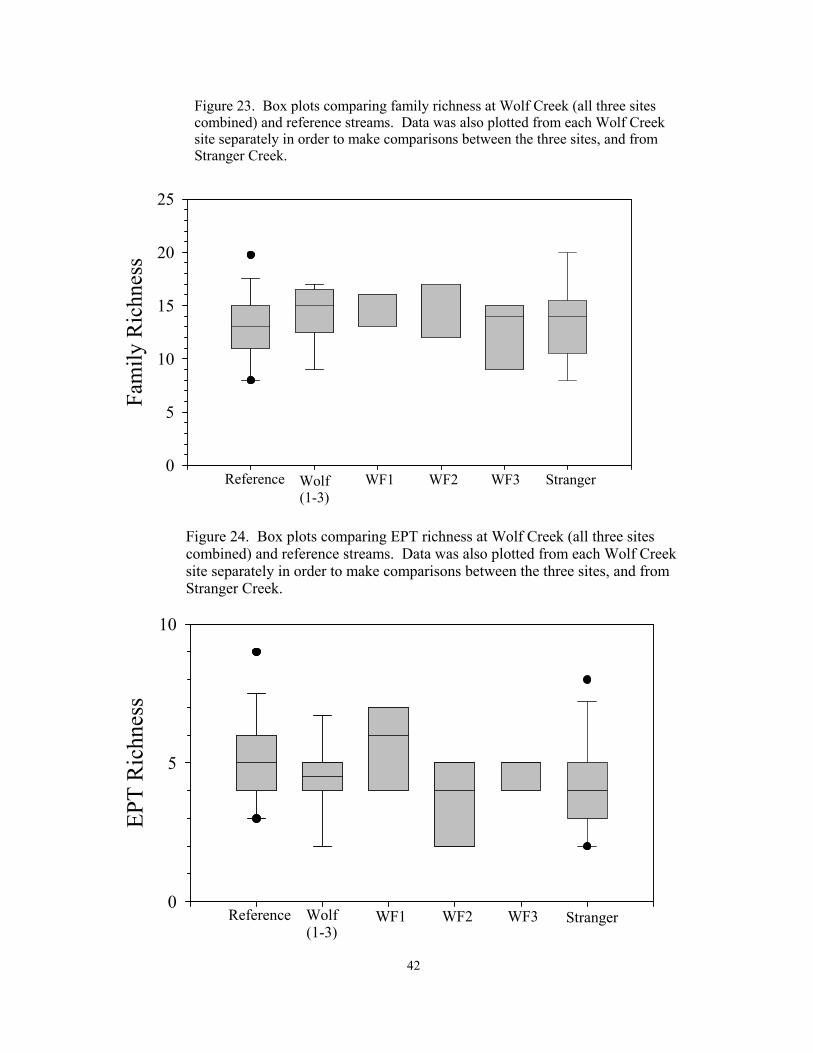
Figure 22. Box plots comparing Habitat Development Index (HDI) at Wolf Creek (all three sites combined) and reference streams. Data was also plotted from each Wolf Creek site separately in order to make comparisons between the three sites....................................................................................................39 Figure 23. Box plots comparing family richness at Wolf Creek (all three sites combined) and reference streams. Data was also plotted from each Wolf Creek site separately in order to make comparisons between the three sites...............………………..42
Figure 24. Box plots comparing EPT richness at Wolf Creek (all three sites combined) and reference streams. Data was also plotted from each Wolf Creek site separately in order to make comparisons between the three sites..............42
Figure 25. Box plots comparing insect abundance at Wolf Creek (all three sites combined) and reference streams. Data was also plotted from each Wolf Creek site separately in order to make comparisons between the three sites..……….43 Figure 26. Box plots comparing EPT abundance at Wolf Creek (all three sites combined) and reference streams. Data was also plotted from each Wolf Creek site separately in order to make comparisons between the three sites. ..........…..……………….44
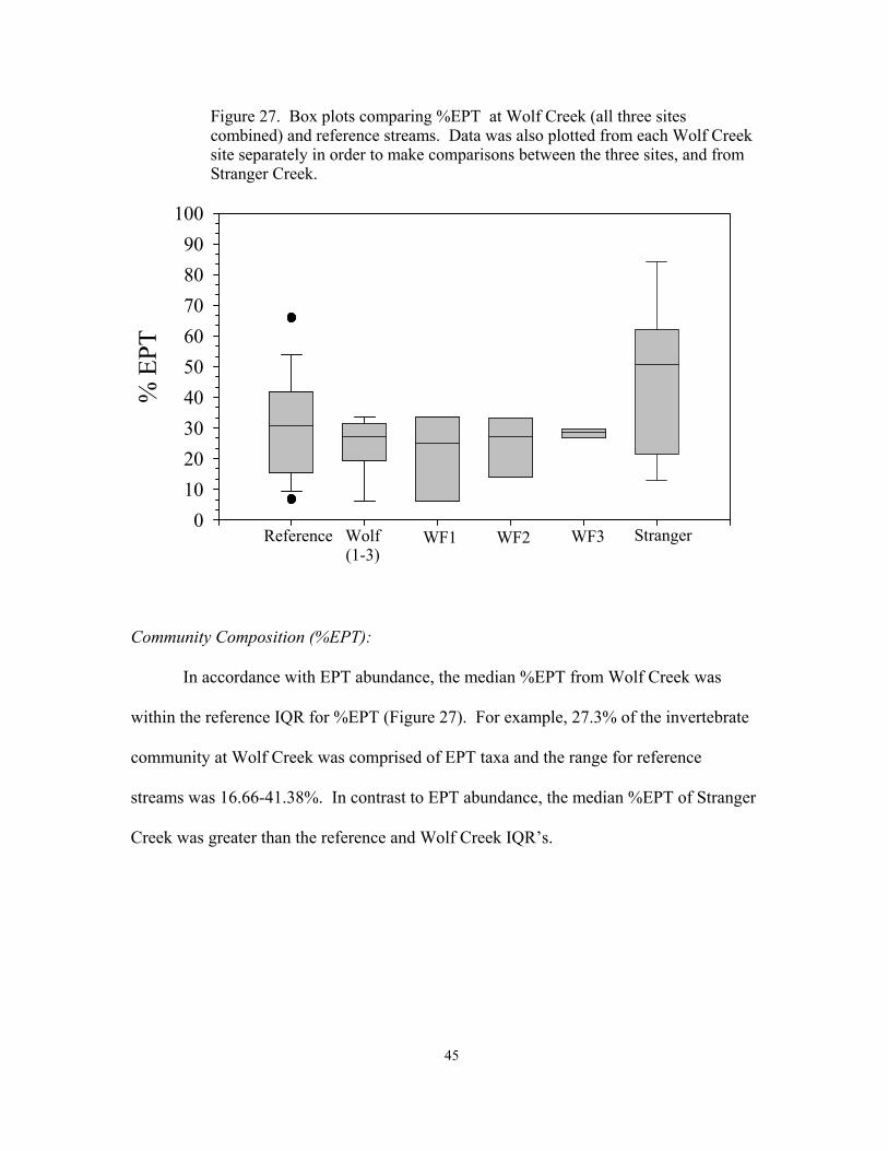
Figure 27. Box plots comparing %EPT at Wolf Creek (all three sites combined) and reference streams. Data was also plotted from each Wolf Creek site separately in order to make comparisons between the three sites.................……………....………....45 Figure 28. Map of the Stranger Creek watershed and the five sites sampled in 2003........…………………………………………………………………… 51
Figure 29. Percent stream bottom cover for inorganic substrate occurring at five StrangerCreek sites sampled in the fall of 2003……………………………….52
Figure 30. Percent stream bottom cover for inorganic substrate occurring at the three Stranger Creek sites in 2001 (Liechti and Dzialowski, 2002)…………………53 Figure 31. Box plots comparing stream shading (%) at the five Stranger Creek sites sampled in 2003, and the three original Stranger Creek sites sampled in 2001 (Liechti and Dzialowski, 2002)……………………………………………….54
5

List of Tables
Table 1. Species lists for all fish collected from Wolf Creek throughout the course of the study………………………………………………….....................35 Table 2. List of all macroinvertebrate families collected from Wolf Creek throughout the course of the study………………………….................…...............41
6
Acknowledgments
This research was completed with the help of many people at KBS and Leavenworth County. Steve Wang and Niang Choo Lim conducted all water quality analysis at the Kansas Biological Survey Ecotoxicology Laboratory. Jeff Anderson, Debbie Baker, Bob Everhart, Clint Goodrich, Don Huggins, Will Spotts, and John Zoellner helped with stream sampling. Clint Goodrich identified all fish samples. Don Huggins and John Zoellner provided general support throughout the project. This project was completed with EPA 319 funds through Leavenworth County.
7
Introduction
Streams and rivers provide many important services to humans including
irrigation, waste dilution, transportation, drinking water, fish for harvest and sport, power
generation, and recreation (Cushing and Allan, 2001). These systems however, are
continuously being disturbed and as a result few unaltered river segments remain in the
United States (U.S. EPA, 1996). For example, the U.S. Environmental Protection
Agency has reported that 36% of the rivers surveyed throughout the United States are
impaired.
Agriculture is a major source of disturbance to streams within the midwestern
United States (U.S. EPA, 1996; Smith, 2003). The application of fertilizers and manure
to farmland has severely degraded the quality of water in rivers in agricultural regions by
creating elevated nutrient loads. While all plants and animals need nutrients, mainly
nitrogen and phosphorus, excess amounts can be detrimental to both humans and aquatic
organisms (Smith, 2003). In addition, riparian forests that buffer streams from their
surrounding watersheds are increasingly being altered or destroyed in order to maximize
the amount of land available for agricultural cultivation. This removal or loss of riparian
forest can result in a number of detrimental stream impacts including increases in
temperature, nutrients, and channel widths, as well as reductions in instream habitat,
increased soil erosion, and increased sedimentation (Allen, 1995).
Bioassessment studies incorporating both spatial and temporal data are often used
to document stream disturbances (Barbour et al., 1999). In this study, the Kansas
Biological Survey (KBS) conducted a biological assessment of the overall ecological
integrity of Wolf Creek, located in Leavenworth County, Kansas. Three sites were
8
selected along Wolf Creek and sampled for a variety of physical, chemical, and
biological variables in the spring, summer, and fall of 2003. Data collected from Wolf
Creek was then compared to similar data collected from streams located within three
reference watersheds. The reference watersheds were previously determined to have high
habitat, water quality, and biological conditions. Due to the increasingly strong presence
of anthropogenic disturbances within the Wolf Creek watershed, this analysis was used to
determine if Wolf Creek has deviated from reference conditions. In addition, it will help
build a framework for future Leavenworth County watershed management plans and
objectives.
The KBS also re-assessed several sites along Stranger Creek, for which we
previously conducted an ecological assessment in 2001 (Liechti and Dzialowski, 2001).
Although fish habitat assessments were originally conducted at Stranger Creek, two of
the three sites were directly below a bridge. Therefore, we re-sampled potential fish
habitat outside the zone of influence of the bridges in order to obtain a more
representative assessment of the habitat available at Stranger Creek.
Watershed Descriptions: Wolf Creek and Reference Streams
The Wolf Creek watershed is located in northeastern Kansas (Figure 1). The
three reference watersheds that will be used in this study are located within the Western
Corn Belt Plains (WCBP) ecoregion and they are roughly the same size as Wolf Creek
and they have similar land use patterns: French (Nemaha County, KS), Straight (Jackson
County, KS), and North Elm (Marshall County, KS). These watersheds were chosen
based on a 1992-1994 KBS study that indicated that they generally had higher habitat and
9

10
water quality, and biological conditions than the streams of 14 other watersheds
examined within the same ecoregion. The use of regional reference condition in
biomonitoring provides an effective framework for assessing and detecting impairment
(Hughes et al., 1986; Barbour et al., 1999)
Data Analysis: Wolf Creek and Reference Streams
In order to compare the physical, biological, and chemical conditions of the Wolf
Creek and the reference watersheds, we graphed the data as box plots. The comparison
of two or more populations using box plots is commonly used in bioassessement studies
(e.g. Karr et al., 1986; Barbour et al., 1999). The horizontal line that divides the box into
two parts is the median value. The upper part of the box represents the 75th percentile of
the data set and the lower part of the box represents the 25th percentile of the data. The
total height of the box therefore represents 50% of the data set, or the interquartile range
(IQR). The whiskers that extend out from the box represent the 5th and 95th percentile of
the data, and additional data points outside of the whiskers represent outliers.
Stream measurements from the three reference watersheds were combined and the
resulting box plot was used as a benchmark of “good” or healthy conditions for each
metric. The median line from the Wolf Creek data was then compared to the IQR values
obtained from the reference watersheds in order to determine if differences exist between
Wolf Creek and the reference watersheds. If the median line of a particular variable fell
within the IQR of the reference watersheds, then the two streams were considered similar
for that particular variable. However, if the median value of a variable collected at Wolf
Creek fell outside of the IQR of the reference watersheds, this suggested that for that
11
particular variable there were potentially significant differences between Wolf Creek and
the reference watersheds.
Sampling of the streams within the three reference watersheds was conducted
using methodology consistent with the sampling of Wolf Creek. Each watershed
contained five stream sites that were sampled in the spring, summer, and fall of 1992,
1993, and 1994. Therefore, each reference stream was sampled 9 times. Efforts were
made to temporally standardize the data sets between Wolf Creek and the reference
watersheds in order to provide a suitable framework for comparison. For example,
winter data collected from the reference streams was not included in our analysis because
we did not collect winter data from Wolf Creek.
There were some differences between Wolf Creek and the reference streams with
respect to the number of samples used to construct the box plots. For example, we
combined all of the data from the three Wolf Creek sites to construct box plots and
therefore each box was based on 9 habitat variables and 27 water quality variables. In
comparison, the box plots constructed for the reference watersheds were based on a much
greater number of samples (15 streams sampled 9 times each). With respect to biotic
samples (macroinvertebrate and fish) we tried to standardize the number of samples
because increased sampling effort usually increases the number of species found.
Therefore we only used biotic data collected from the 15 reference streams from one year
(spring, summer, and fall), which corresponds to the same level of sampling effort used
for Wolf Creek.
We also plotted the data from each of the three Wolf Creek sites separately in
order to determine if there were differences between sites. There were only three data
12
points for some of the habitat variables however, and in these instances the results should
be interpreted with caution. Finally, we plotted data collected from Stranger Creek in our
initial analysis conducted in 2001 using similar methodology (Liechti and Dzialowski,
2002) to see if differences exist between Wolf and Stranger Creek’s.
Sampling: Wolf Creek
Three sites were selected for analysis on Wolf Creek (Figure 1). Caution was
taken when selecting these sites so that they were out of the influence of bridges. Each
site was sampled during three individual sampling events one each in the spring (6 June),
the summer (22 July) and the fall (9 October) of 2003.
At each site a 50 m segment of stream was divided into three sections (upper,
middle, and lower), each of which represented a distinct macrohabitat (run, riffle, or
pool) when available. All three of these macrohabitats were present at each site during
the first sampling event. However, on subsequent sampling events they were not always
preset, and the available habitat was sampled. The physical, biological, and ecological
conditions of Wolf Creek were then assessed using methodology from Platts et al.,
(1987) and Barbour et al., (1999).
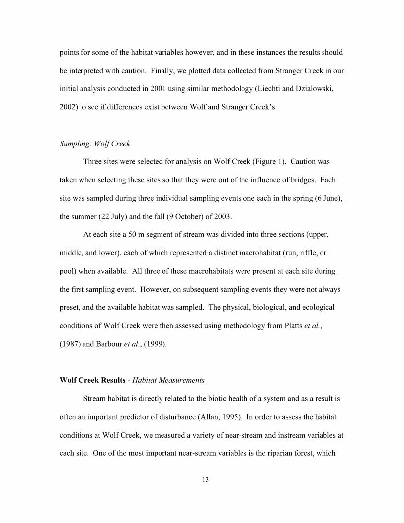
Wolf Creek Results - Habitat Measurements
Stream habitat is directly related to the biotic health of a system and as a result is
often an important predictor of disturbance (Allan, 1995). In order to assess the habitat
conditions at Wolf Creek, we measured a variety of near-stream and instream variables at
each site. One of the most important near-stream variables is the riparian forest, which
13
provides an effective buffer between streams and their catchments (Kalff, 2002). The
alteration of riparian forest often results from agricultural activity where forests are cut to
the river or stream edge in order to maximize the amount of land available for cultivation
(Kalff, 2002). The overall riparian forest at each Wolf Creek site was assessed based on
several variables including stream shading, riparian width, and riparian condition.
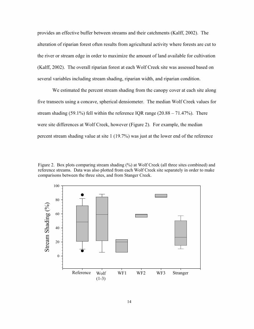
We estimated the percent stream shading from the canopy cover at each site along
five transects using a concave, spherical densiometer. The median Wolf Creek values for
stream shading (59.1%) fell within the reference IQR range (20.88 – 71.47%). There
were site differences at Wolf Creek, however (Figure 2). For example, the median
percent stream shading value at site 1 (19.7%) was just at the lower end of the reference
Stre
am S
hadi
ng (%
)
0
20
40
60
80
100
WF1 WF2 WF3Wolf(1-3)
Reference
Figure 2. Box plots comparing stream shading (%) at Wolf Creek (all three sites combined) and reference streams. Data was also plotted from each Wolf Creek site separately in order to makecomparisons between the three sites, and from Stanger Creek.
Stranger
14
IQR, and the median value for site 3 (84.1%) was greater than the reference IQR. In
addition, the median percent stream shading value for Wolf Creek was greater than the
IQR for Stranger Creek (15.05 – 50.3%).
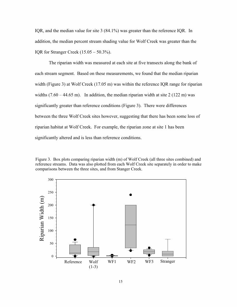
The riparian width was measured at each site at five transects along the bank of
each stream segment. Based on these measurements, we found that the median riparian
width (Figure 3) at Wolf Creek (17.05 m) was within the reference IQR range for riparian
widths (7.60 – 44.65 m). In addition, the median riparian width at site 2 (122 m) was
significantly greater than reference conditions (Figure 3). There were differences
between the three Wolf Creek sites however, suggesting that there has been some loss of
riparian habitat at Wolf Creek. For example, the riparian zone at site 1 has been
significantly altered and is less than reference conditions.
Rip
aria
n W
idth
(m)
0
50
100
150
200
250
300
WF1 WF2 WF3Wolf(1-3)
Reference
Figure 3. Box plots comparing riparian width (m) of Wolf Creek (all three sites combined) and reference streams. Data was also plotted from each Wolf Creek site separately in order to makecomparisons between the three sites, and from Stanger Creek.
Stranger
15
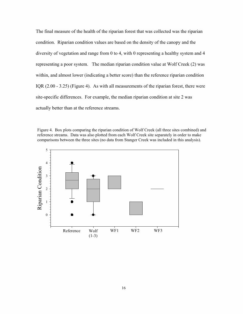
The final measure of the health of the riparian forest that was collected was the riparian
condition. Riparian condition values are based on the density of the canopy and the
diversity of vegetation and range from 0 to 4, with 0 representing a healthy system and 4
representing a poor system. The median riparian condition value at Wolf Creek (2) was
within, and almost lower (indicating a better score) than the reference riparian condition
IQR (2.00 - 3.25) (Figure 4). As with all measurements of the riparian forest, there were
site-specific differences. For example, the median riparian condition at site 2 was
actually better than at the reference streams.
Rip
aria
n C
ondi
tion
0
1
2
3
4
5
WF1 WF2 WF3Wolf(1-3)
Reference
Figure 4. Box plots comparing the riparian condition of Wolf Creek (all three sites combined) and reference streams. Data was also plotted from each Wolf Creek site separately in order to makecomparisons between the three sites (no data from Stanger Creek was included in this analysis).
16

To determine if there were differences in erosion between Wolf Creek and
reference streams, we measured the length and average height of all areas of active bank
erosion and calculated the total area of bank erosion at each site. Based on this analysis,
we found that the amount of active erosion at Wolf Creek was similar to the amount of
active erosion at the reference streams (Figure 5). The median value for erosion area at
Wolf Creek was 27.4 m2 compared to the IQR range for reference streams that was 0 –
36.75 m2. Similar to other habitat measures however, the median active erosion value for
site 1 (74.2 m2) was significantly higher than the reference IQR. Stream bank erosion
can lead to direct soil loss, and a resulting increase in turbidity.
Eros
iona
l Are
a (m
2 )
0
50
100
150
200
250
300
WF1 WF2 WF3Wolf(1-3)
Reference
Figure 5. Box plots comparing erosion at Wolf Creek (all three sites combined) and reference streams. Data was also plotted from each Wolf Creek site separately in order to make comparisons between the three sites, and from Stranger Creek.
Stranger
17

Channel widths were measured at five transects at each site. Overall, the median
channel width from the three Wolf Creek sites (18.0 m) was within the reference IQR for
channel widths (12.8 – 19.1 m). However, the median channel width at site 1 (27.4 m)
was significantly larger than the reference IQR, and was similar to the channel widths
observed at Stranger Creek in 2001 (Figure 6). Increased channel widths likely result
from reductions in riparian habitat quality and quantity (see Figure 3).
Cha
nnel
Wid
th (m
)
0
10
20
30
40
50
60
WF1 WF2 WF3Wolf(1-3)
Reference Stranger
Figure 6. Box plots comparing erosion at Wolf Creek (all three sites combined) and reference streams. Data was also plotted from each Wolf Creek site separately in order to make comparisons between the three sites, and from Stranger Creek.
18

Inorganic substrate values (% cover) were recorded at each site to determine if
there were differences in the substrate heterogeneity between Wolf Creek and the
reference streams. Transects were established along each available macrohabitat, and the
type of substrate that was present at 30 points within the section were measured. The
overall inorganic substrate composition at all Wolf Creek sites combined was very
diverse compared to that of the reference streams (Figure 7). The major substrate types
present at Wolf Creek include cobble (33%), sand (10%), soft silt (26%), bedrock (15%),
gravel (11%) (Figure 7). In addition, there was little difference between the three Wolf
Creek sites as each was dominated by cobble. A major difference in the substrate
between the three sites was the presence of a large amount of bedrock at site 2 (42%). In
contrast, a single substrate type dominated the reference streams. Straight and French
were dominated by sand (66.6% and 63.0% respectively) and North Elm was dominated
by cobble (58.8%). Therefore, Wolf Creek has a more diverse inorganic substrate then
the reference streams, which is directly related to biotic diversity (Allen, 1995).
19

Figure 7. Percent stream bottom cover for inorganic substrate occurring at Wolf Creek (all three sites combined). Data was also plotted from each Wolf Creek site separately in order to make comparisons between the three sites.
Site 3
Cobble28%
Gravel10%
Sand17%
Hard Clay/Mud
0%
Soft Silt44%
Bedrock1%
Wolf Creek (1-3)
Bedrock15%
Cobble33%
Gravel10%
Sand10%
Hard Clay/Mud
6%
Soft Silt26%
Site 2Soft Silt
10%
Hard Clay/Mud
3%
Bedrock43%
Cobble38%
Gravel
Site 3
Cobble28%
Gravel10%
Sand17%
Hard Clay/Mud
0%
Soft Silt44%
Bedrock1%
20
Water Quality:
In order to assess the water quality at Wolf Creek, a total of three grab samples
were collected from each site (upper, middle, and lower) on each sampling date. The
samples were taken back to the Ecotoxicology Laboratory at the KBS where they were
analyzed for total phosphorus and nitrogen, alkalinity, hardness, chemical oxygen
demand, fecal coliform concentrations, and atrazine a pesticide that is commonly used in
this ecoregion. During each sample event we also used an Horiba H20 multi-probe water
quality analyzer to record in situ measurements of pH, turbidity (NTU), conductivity
(uohms), and dissolved oxygen (mg/l) at each site.
pH data collected at Wolf Creek shows that there was no difference between Wolf
Creek and the reference streams. For example, the median pH value at Wolf Creek was
7.77, which was within the pH IQR range for the reference streams (7.64 – 8.19) (Figure
8). Median pH values were lower at site 1 although only slightly (7.64). These median
values are all within the Kansas surface water criteria for maintenance of aquatic life
(6.50 - 8.50) suggesting that Wolf Creek has not experienced degradation with respect to
pH. This was in contrast to our initial study of Stranger Creek, in which we found that
median pH values (8.34) collected from Stranger Creek were higher than reference
streams and near the upper limits of the Kansas surface water criteria.
Turbidity values were higher in Wolf Creek than in reference streams (Figure 9).
The overall Wolf Creek median turbidity value (82 NTU), as well as the median turbidity
values for two of the three sites were greater than the reference IQR (7 – 50 NTU). Site 1
was the only site that had turbidity values similar to reference condition. The median
turbidity value for all Wolf Creek sites combined was also very similar to the median
21

pH
7.4
7.6
7.8
8.0
8.2
8.4
8.6
8.8
WF1 WF2 WF3Wolf(1-3)
Reference
Figure 8. Box plots comparing pH at Wolf Creek (all three sites combined) and reference streams. Data was also plotted from each Wolf Creek site separately in order to makecomparisons between the three sites, and for Stranger Creek.
Stranger
Turb
idity
(NTU
)
0
100
200
300
WF1 WF2 WF3Wolf(1-3)
Reference
Figure 9. Box plots comparing turbidity at Wolf Creek (all three sites combined) and reference streams. Data was also plotted from each Wolf Creek site separately in order to makecomparisons between the three sites, and from Stanger Creek.
Stranger
22
turbidity value collected from Stranger Creek (81 NTU) in our initial analysis. The
Kansas surface water quality standards for turbidity suggest that increased suspended
solid levels shall not impair the behavior, reproduction, physical habitat or any other
factors related to any organism utilizing surface water systems. Elevated turbidity likely
results from increases in sediment load from the watershed or high rates of stream bed
and bank erosion, and can lead to shifts in the species composition of stream biota (Allan,
1995).
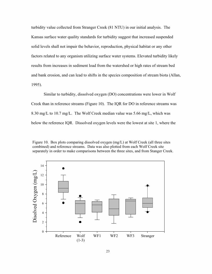
Similar to turbidity, dissolved oxygen (DO) concentrations were lower in Wolf
Creek than in reference streams (Figure 10). The IQR for DO in reference streams was
8.30 mg/L to 10.7 mg/L. The Wolf Creek median value was 5.66 mg/L, which was
below the reference IQR. Dissolved oxygen levels were the lowest at site 1, where the
Dis
olve
d O
xyge
n (m
g/L)
0
2
4
6
8
10
12
14
WF1 WF2 WF3Wolf(1-3)
Reference
Figure 10. Box plots comparing dissolved oxygen (mg/L) at Wolf Creek (all three sites combined) and reference streams. Data was also plotted from each Wolf Creek site separately in order to make comparisons between the three sites, and from Stanger Creek.
Stranger
23
median concentration (4.82 mg/L) was slightly below the Kansas surface water standard,
which is set at 5.0 mg/L. The observed low DO levels in Wolf Creek may be the result of
low primary productivity resulting from increased turbidity values (Figure 9). In
addition, low DO levels may be the result of increased decomposition due to high inputs
of organic matter from the watershed. However, these low values may have resulted
from the presence of isolated pools at Wolf Creek due to periods of low flow observed
throughout the study. These pools experience a high level of decomposition, but are not
refreshed with oxygenated water from upstream. While it is difficult to determine the
actual causes of the observed low DO values at Wolf Creek, the recorded values were
below reference values and near the lower limit of the Kansas surface water standards.
Therefore, more intense sampling and monitoring may be necessary to determine how
degraded Wolf Creek has become with respect to DO concentrations, and the causes for
this degradation.
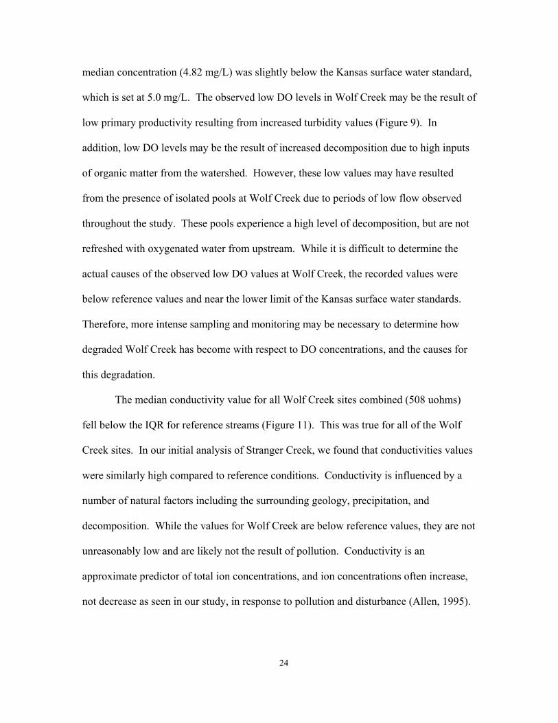
The median conductivity value for all Wolf Creek sites combined (508 uohms)
fell below the IQR for reference streams (Figure 11). This was true for all of the Wolf
Creek sites. In our initial analysis of Stranger Creek, we found that conductivities values
were similarly high compared to reference conditions. Conductivity is influenced by a
number of natural factors including the surrounding geology, precipitation, and
decomposition. While the values for Wolf Creek are below reference values, they are not
unreasonably low and are likely not the result of pollution. Conductivity is an
approximate predictor of total ion concentrations, and ion concentrations often increase,
not decrease as seen in our study, in response to pollution and disturbance (Allen, 1995).
24
Con
duct
ivity
(um
hos)
400
500
600
700
800
WF1 WF2 WF3Wolf(1-3)
Reference
Figure 11. Box plots comparing conductivity (uohms) at Wolf Creek (all three sites combined) and reference streams. Data was also plotted from each Wolf Creek site separately in order to make comparisons between the three sites, and from Stranger Creek.
Stranger
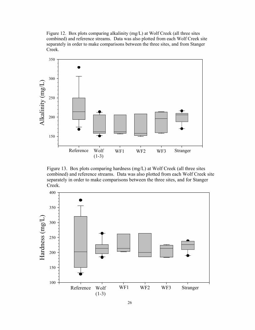
Alkalinity concentrations in Wolf Creek were lower than in the reference streams
(Figure 12). The IQR for the reference streams was 194 – 250 mg/L as CaCO3 and the
median value from all of the Wolf Creek sites combined was 162 mg/L. Similarly,
Alkalinity was higher in our 2002 analysis of Stranger Creek (IQR = 188 – 210) than in
Wolf Creek. Alkalinity is a measure of the acid-neutralizing capacity of water, and is
greatly influenced by the surrounding geology. Streams located in this area are naturally
buffered due to high levels of bicarbonate within the surface geology, and similar to pH,
these differences do not likely reflect disturbance or degradation.
In contrast to alkalinity values, there were no differences between Wolf Creek and
reference streams with respect to hardness (Figure 13). The median value for all Wolf
25
Alk
alin
ity (m
g/L)
150
200
250
300
350
WF1 WF2 WF3Wolf(1-3)
Reference
Figure 12. Box plots comparing alkalinity (mg/L) at Wolf Creek (all three sites combined) and reference streams. Data was also plotted from each Wolf Creek site separately in order to make comparisons between the three sites, and from StangerCreek.
Stranger
26
Har
dnes
s (m
g/L)
100
150
200
250
300
350
400
WF1 WF2 WF3Wolf(1-3)
Reference
Figure 13. Box plots comparing hardness (mg/L) at Wolf Creek (all three sites combined) and reference streams. Data was also plotted from each Wolf Creek site separately in order to make comparisons between the three sites, and for StangerCreek.
Stranger
Creek sites combined (214 mg/L) fell within the IQR from reference streams (150 – 320
mg/L). Hardness is primarily a measure of the amount of calcium and magnesium salts
within the water (Allen, 1995) and as with alkalinity is highly influenced by the
surrounding geology.
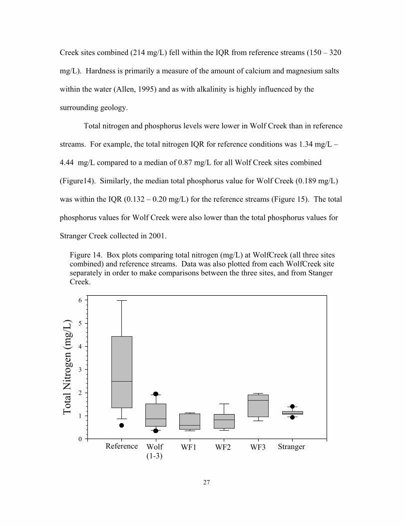
Total nitrogen and phosphorus levels were lower in Wolf Creek than in reference
streams. For example, the total nitrogen IQR for reference conditions was 1.34 mg/L –
4.44 mg/L compared to a median of 0.87 mg/L for all Wolf Creek sites combined
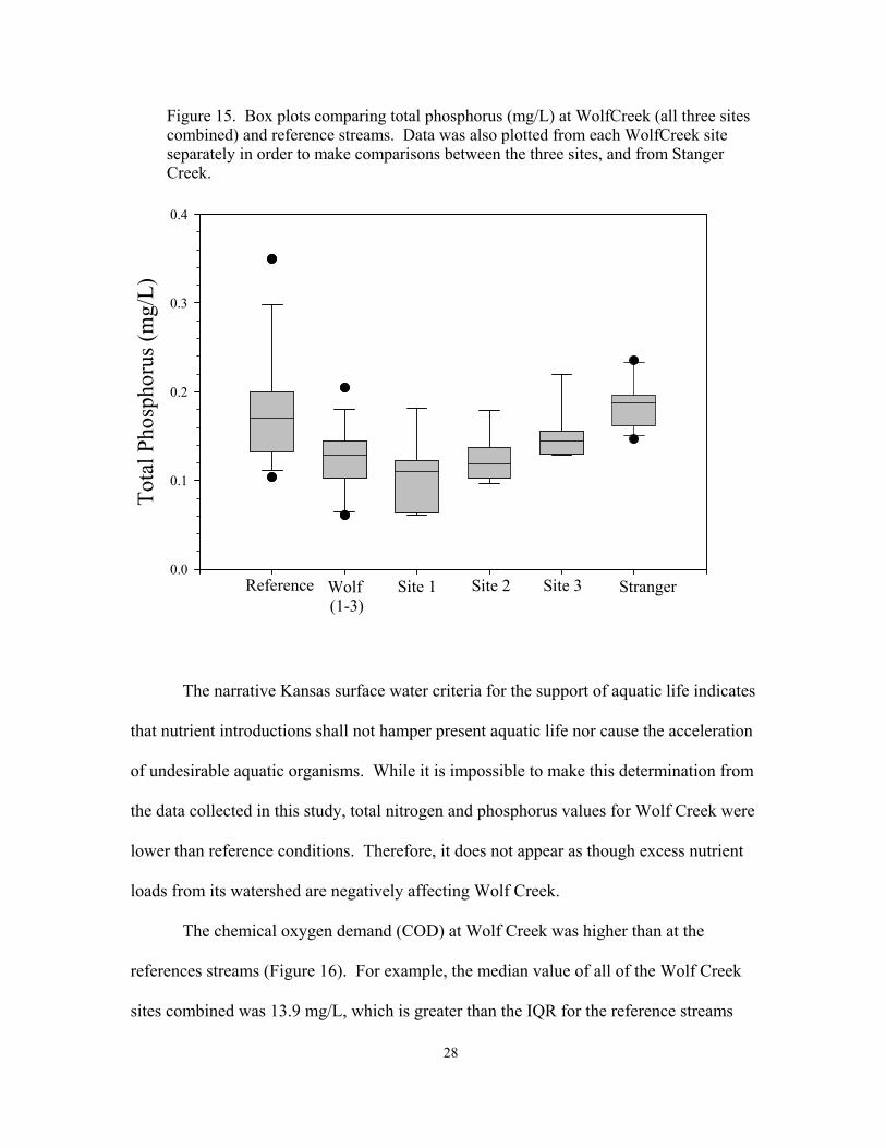
(Figure14). Similarly, the median total phosphorus value for Wolf Creek (0.189 mg/L)
was within the IQR (0.132 – 0.20 mg/L) for the reference streams (Figure 15). The total
phosphorus values for Wolf Creek were also lower than the total phosphorus values for
Stranger Creek collected in 2001.
Tota
l Nitr
ogen
(mg/
L)
0
1
2
3
4
5
6
WF1 WF2 WF3Wolf(1-3)
Reference
Figure 14. Box plots comparing total nitrogen (mg/L) at WolfCreek (all three sites combined) and reference streams. Data was also plotted from each WolfCreek site separately in order to make comparisons between the three sites, and from Stanger Creek.
Stranger
27
Tota
l Pho
spho
rus (
mg/
L)
0.0
0.1
0.2
0.3
0.4
Stranger Site 2 Site 3Wolf (1-3)
Reference Site 1
Figure 15. Box plots comparing total phosphorus (mg/L) at WolfCreek (all three sites combined) and reference streams. Data was also plotted from each WolfCreek site separately in order to make comparisons between the three sites, and from Stanger Creek.
The narrative Kansas surface water criteria for the support of aquatic life indicates
that nutrient introductions shall not hamper present aquatic life nor cause the acceleration
of undesirable aquatic organisms. While it is impossible to make this determination from
the data collected in this study, total nitrogen and phosphorus values for Wolf Creek were
lower than reference conditions. Therefore, it does not appear as though excess nutrient
loads from its watershed are negatively affecting Wolf Creek.
The chemical oxygen demand (COD) at Wolf Creek was higher than at the
references streams (Figure 16). For example, the median value of all of the Wolf Creek
sites combined was 13.9 mg/L, which is greater than the IQR for the reference streams
28
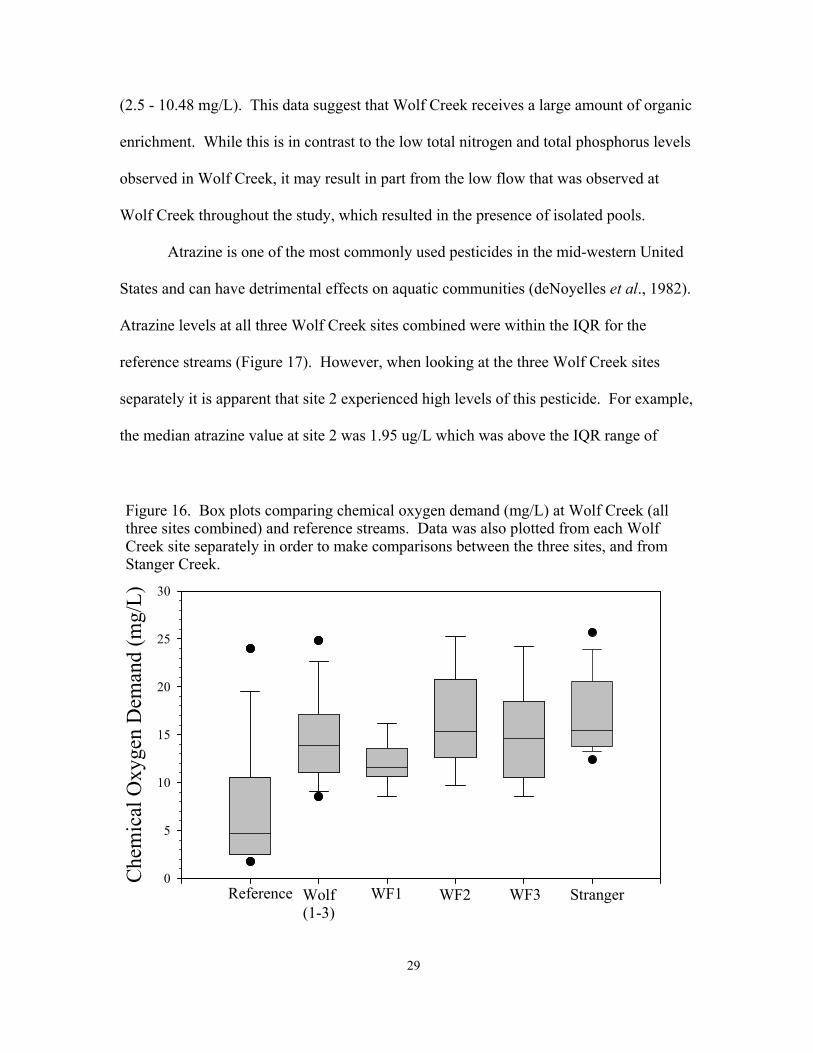
(2.5 - 10.48 mg/L). This data suggest that Wolf Creek receives a large amount of organic
enrichment. While this is in contrast to the low total nitrogen and total phosphorus levels
observed in Wolf Creek, it may result in part from the low flow that was observed at
Wolf Creek throughout the study, which resulted in the presence of isolated pools.
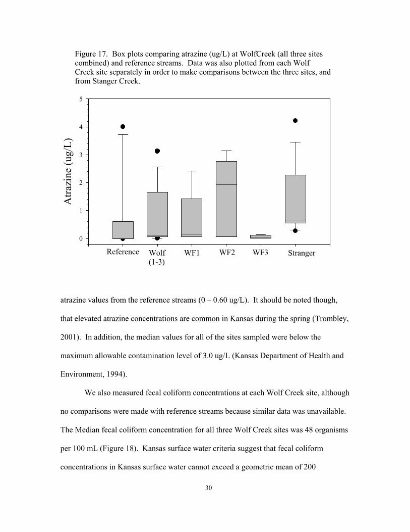
Atrazine is one of the most commonly used pesticides in the mid-western United
States and can have detrimental effects on aquatic communities (deNoyelles et al., 1982).
Atrazine levels at all three Wolf Creek sites combined were within the IQR for the
reference streams (Figure 17). However, when looking at the three Wolf Creek sites
separately it is apparent that site 2 experienced high levels of this pesticide. For example,
the median atrazine value at site 2 was 1.95 ug/L which was above the IQR range of
Che
mic
al O
xyge
n D
eman
d (m
g/L)
0
5
10
15
20
25
30
WF1 WF2 WF3Wolf(1-3)
Reference
Figure 16. Box plots comparing chemical oxygen demand (mg/L) at Wolf Creek (all three sites combined) and reference streams. Data was also plotted from each WolfCreek site separately in order to make comparisons between the three sites, and from Stanger Creek.
Stranger
29
Atra
zine
(ug/
L)
0
1
2
3
4
5
WF1 WF2 WF3Reference
Figure 17. Box plots comparing atrazine (ug/L) at WolfCreek (all three sites combined) and reference streams. Data was also plotted from each WolfCreek site separately in order to make comparisons between the three sites, andfrom Stanger Creek.
StrangerWolf(1-3)
atrazine values from the reference streams (0 – 0.60 ug/L). It should be noted though,
that elevated atrazine concentrations are common in Kansas during the spring (Trombley,
2001). In addition, the median values for all of the sites sampled were below the
maximum allowable contamination level of 3.0 ug/L (Kansas Department of Health and
Environment, 1994).
We also measured fecal coliform concentrations at each Wolf Creek site, although
no comparisons were made with reference streams because similar data was unavailable.
The Median fecal coliform concentration for all three Wolf Creek sites was 48 organisms
per 100 mL (Figure 18). Kansas surface water criteria suggest that fecal coliform
concentrations in Kansas surface water cannot exceed a geometric mean of 200
30
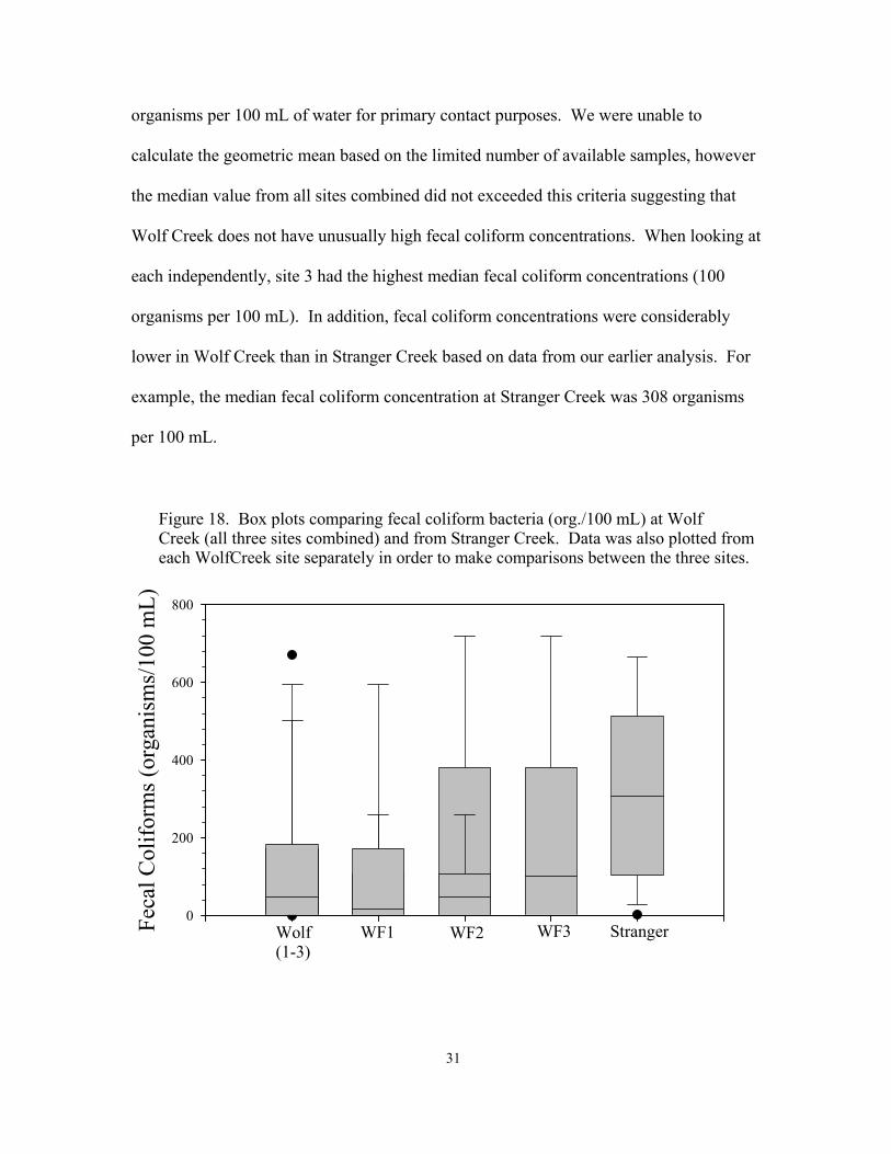
organisms per 100 mL of water for primary contact purposes. We were unable to
calculate the geometric mean based on the limited number of available samples, however
the median value from all sites combined did not exceeded this criteria suggesting that
Wolf Creek does not have unusually high fecal coliform concentrations. When looking at
each independently, site 3 had the highest median fecal coliform concentrations (100
organisms per 100 mL). In addition, fecal coliform concentrations were considerably
lower in Wolf Creek than in Stranger Creek based on data from our earlier analysis. For
example, the median fecal coliform concentration at Stranger Creek was 308 organisms
per 100 mL.
Feca
l Col
iform
s (or
gani
sms/
100
mL)
0
200
400
600
800
WF1 WF2 WF3
Figure 18. Box plots comparing fecal coliform bacteria (org./100 mL) at Wolf Creek (all three sites combined) and from Stranger Creek. Data was also plotted from each WolfCreek site separately in order to make comparisons between the three sites.
Wolf(1-3)
Stranger
31
Biota:
Three primary biological variables were measured at each site: periphyton,
macroinvertebrates, and fish. Each of these variables is a valuable indicator of water
quality (Barbour et al., 1999).
Periphyton:
Benthic algae, or periphyton, is the most important source of primary production
in streams. Algal communities are strongly affected by nutrient enrichment and
disturbance, and therefore are a valuable indicator of ecosystem health (Barbour et al.,
1999). Periphyton samples were collected in triplicate from the dominant substrate type
at each habitat. The substrate was isolated with a gasketed sampling tube and agitated
with a brush. The dislodged material was removed by aspirating into a 40 ml collection
vial. The samples were then returned to the Ecotoxicology Laboratory where
concentrations of chlorophyll a and pheophytin a, two photosynthetic plant pigments,
were determined fluorometrically. Periphyton was not compared to reference streams
due to differences in sampling methodology. However, we did compare the three Wolf
Creek sites with data collected from Stranger Creek in 2001, in order to determine if
differences existed in concentrations between Wolf and Stranger Creeks.
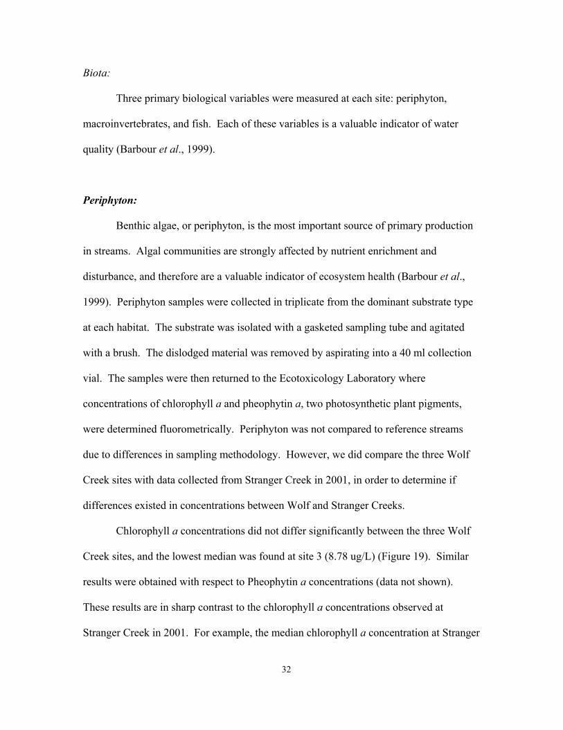
Chlorophyll a concentrations did not differ significantly between the three Wolf
Creek sites, and the lowest median was found at site 3 (8.78 ug/L) (Figure 19). Similar
results were obtained with respect to Pheophytin a concentrations (data not shown).
These results are in sharp contrast to the chlorophyll a concentrations observed at
Stranger Creek in 2001. For example, the median chlorophyll a concentration at Stranger
32
Creek was 45.3 ug/L. In addition the IQR range of chlorophyll a values in Stranger
Creek was 34.0 – 105.2 ug/L. These results suggest that nutrient enrichment has a greater
impact on Stranger Creek than Wolf Creek, a finding that further supports the nutrient
data (Figures 14, 15).
Chl
orop
hyll
a (u
g/L)
0
20
40
60
80
100
120
140
160
WF1 WF2 WF3
Figure 19. Box plots comparing chlorophyll a (ug/L) concentrations from the three WolfCreek sites and Stanger Creek.
StrangerWolf(1-3)
Fish Community:
Samples were collected from each site for analysis of community structure.
Representative portions of the available macrohabitats were individually blocked off and
sampled first with seines and then electrofished with a backpack shocker. Fish samples
33
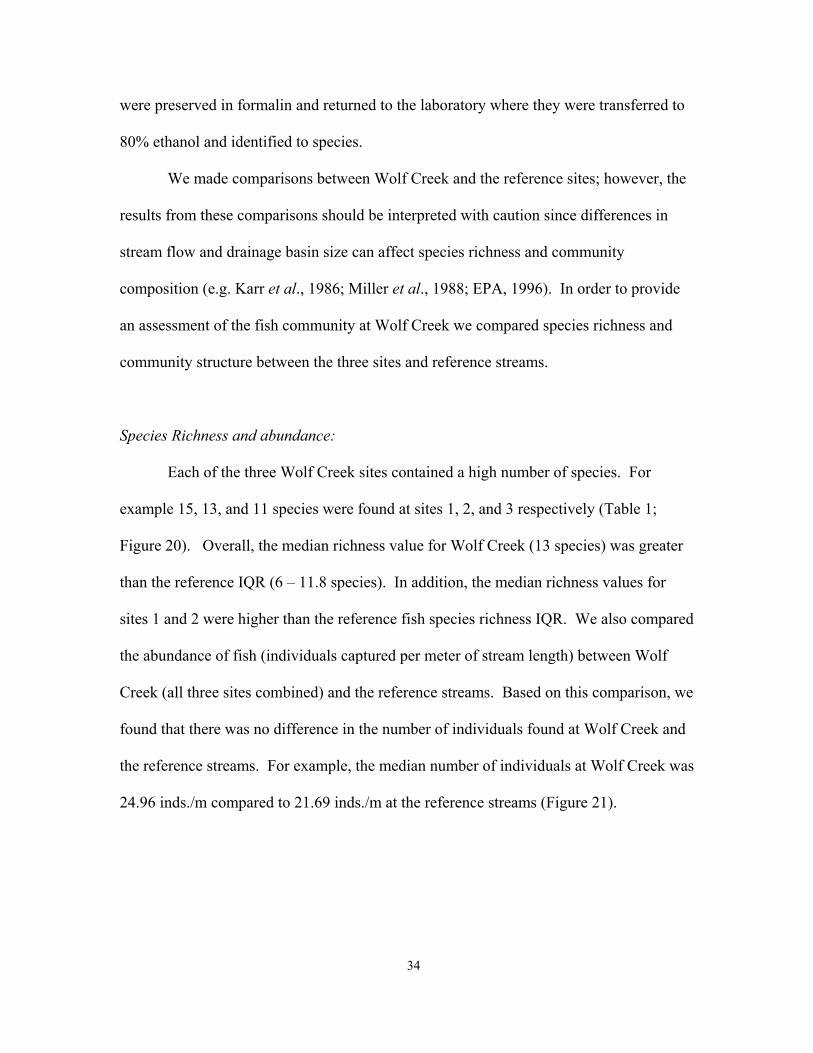
were preserved in formalin and returned to the laboratory where they were transferred to
80% ethanol and identified to species.
We made comparisons between Wolf Creek and the reference sites; however, the
results from these comparisons should be interpreted with caution since differences in
stream flow and drainage basin size can affect species richness and community
composition (e.g. Karr et al., 1986; Miller et al., 1988; EPA, 1996). In order to provide
an assessment of the fish community at Wolf Creek we compared species richness and
community structure between the three sites and reference streams.
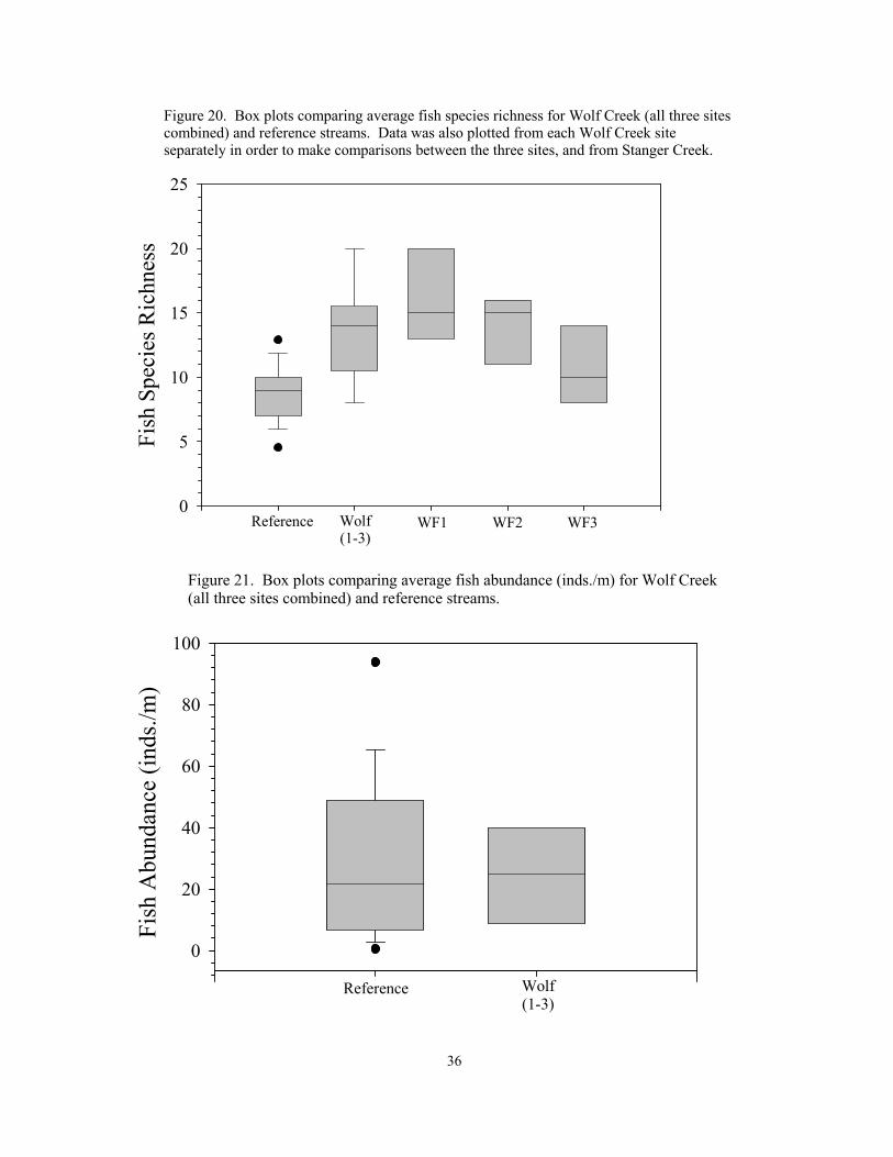
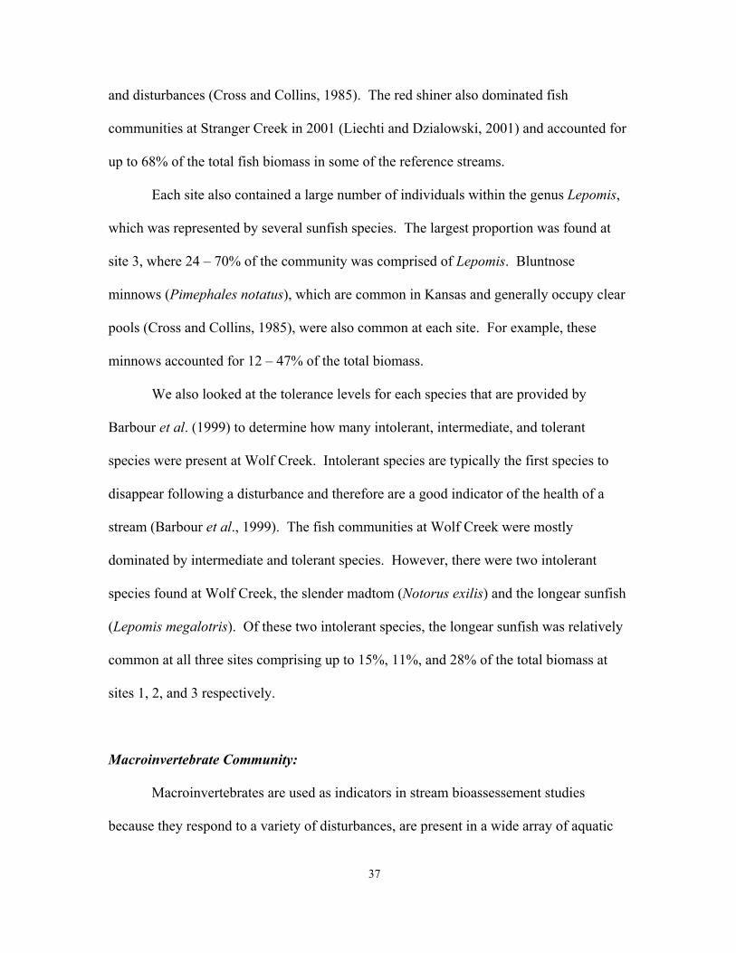
Species Richness and abundance:
Each of the three Wolf Creek sites contained a high number of species. For
example 15, 13, and 11 species were found at sites 1, 2, and 3 respectively (Table 1;
Figure 20). Overall, the median richness value for Wolf Creek (13 species) was greater
than the reference IQR (6 – 11.8 species). In addition, the median richness values for
sites 1 and 2 were higher than the reference fish species richness IQR. We also compared
the abundance of fish (individuals captured per meter of stream length) between Wolf
Creek (all three sites combined) and the reference streams. Based on this comparison, we
found that there was no difference in the number of individuals found at Wolf Creek and
the reference streams. For example, the median number of individuals at Wolf Creek was
24.96 inds./m compared to 21.69 inds./m at the reference streams (Figure 21).
34
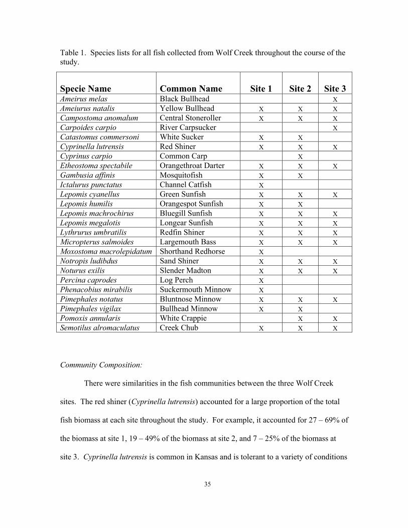
Table 1. Species lists for all fish collected from Wolf Creek throughout the course of the study.
Specie Name Common Name Site 1 Site 2 Site 3
Ameirus melas Black Bullhead X Ameiurus natalis Yellow Bullhead X X X Campostoma anomalum Central Stoneroller X X X Carpoides carpio River Carpsucker X Catastomus commersoni White Sucker X X Cyprinella lutrensis Red Shiner X X X Cyprinus carpio Common Carp X Etheostoma spectabile Orangethroat Darter X X X Gambusia affinis Mosquitofish X X Ictalurus punctatus Channel Catfish X Lepomis cyanellus Green Sunfish X X X Lepomis humilis Orangespot Sunfish X X Lepomis machrochirus Bluegill Sunfish X X X Lepomis megalotis Longear Sunfish X X X Lythrurus umbratilis Redfin Shiner X X X Micropterus salmoides Largemouth Bass X X X Moxostoma macrolepidatum Shorthand Redhorse X Notropis ludibdus Sand Shiner X X X Noturus exilis Slender Madton X X X Percina caprodes Log Perch X Phenacobius mirabilis Suckermouth Minnow X Pimephales notatus Bluntnose Minnow X X X Pimephales vigilax Bullhead Minnow X X Pomoxis annularis White Crappie X X Semotilus alromaculatus Creek Chub X X X
Community Composition:
There were similarities in the fish communities between the three Wolf Creek
sites. The red shiner (Cyprinella lutrensis) accounted for a large proportion of the total
fish biomass at each site throughout the study. For example, it accounted for 27 – 69% of
the biomass at site 1, 19 – 49% of the biomass at site 2, and 7 – 25% of the biomass at
site 3. Cyprinella lutrensis is common in Kansas and is tolerant to a variety of conditions
35
Fish
Spe
cies
Ric
hnes
s
0
5
10
15
20
25
WF1 WF2 WF3Wolf(1-3)
Reference
Figure 20. Box plots comparing average fish species richness for Wolf Creek (all three sites combined) and reference streams. Data was also plotted from each Wolf Creek site separately in order to make comparisons between the three sites, and from Stanger Creek.
Fish
Abu
ndan
ce (i
nds./
m)
0
20
40
60
80
100
Wolf(1-3)
Reference
Figure 21. Box plots comparing average fish abundance (inds./m) for Wolf Creek (all three sites combined) and reference streams.
36
and disturbances (Cross and Collins, 1985). The red shiner also dominated fish
communities at Stranger Creek in 2001 (Liechti and Dzialowski, 2001) and accounted for
up to 68% of the total fish biomass in some of the reference streams.
Each site also contained a large number of individuals within the genus Lepomis,
which was represented by several sunfish species. The largest proportion was found at
site 3, where 24 – 70% of the community was comprised of Lepomis. Bluntnose
minnows (Pimephales notatus), which are common in Kansas and generally occupy clear
pools (Cross and Collins, 1985), were also common at each site. For example, these
minnows accounted for 12 – 47% of the total biomass.
We also looked at the tolerance levels for each species that are provided by
Barbour et al. (1999) to determine how many intolerant, intermediate, and tolerant
species were present at Wolf Creek. Intolerant species are typically the first species to
disappear following a disturbance and therefore are a good indicator of the health of a
stream (Barbour et al., 1999). The fish communities at Wolf Creek were mostly
dominated by intermediate and tolerant species. However, there were two intolerant
species found at Wolf Creek, the slender madtom (Notorus exilis) and the longear sunfish
(Lepomis megalotris). Of these two intolerant species, the longear sunfish was relatively
common at all three sites comprising up to 15%, 11%, and 28% of the total biomass at
sites 1, 2, and 3 respectively.
Macroinvertebrate Community:
Macroinvertebrates are used as indicators in stream bioassessement studies
because they respond to a variety of disturbances, are present in a wide array of aquatic
37
habitats, are relatively easy to sample and process, have long life histories, and are
relatively sedentary (Berkman et al., 1986; Rosenberg and Resh, 1996; Barbour et al.,
1999; Whiles et al., 2001). Disturbances of macroinvertebrate communities may result in
reduced taxa richness, and/or shifts in community composition. In addition, most taxa
within the orders Ephemeroptera, Plecoptera, and Tricoptera (EPT) are sensitive to slight
perturbations in water quality, and their absence can be an effective indicator of
disturbance (Rosenberg and Resh, 1996).
Three macroinvertebrates samples were collected at each site from the available
macrohabitats (e.g. one each in riffle, run, and pool) during each sampling event. In
instances where all of these macrohabitats were not present at a single site, the existing
macrohabitat(s) was subdivided and a sample was collected from each of the
subdivisions. For each sample the substrate was disturbed during a one-minute kick
sample and a D-net was used to collect the dislodged insects. Attempts were made to
sample all microhabitats capable of supporting benthic invertebrates. The
macroinvertebrate samples were preserved in formalin with rose bengal and returned to
the laboratory where they were sorted from the detritus and substrate and identified to
family.
Macroinvertebrate Habitat:
The quality and quantity of stream habitat is an important predictor of invertebrate
community composition (Huggins and Moffett, 1988; Allan, 1995). Therefore a Habitat
Development Index (HDI) was calculated for each site to determine the quality of habitat
at each site (Huggins and Moffett, 1988). The HDI provides a rank of quality for each
38
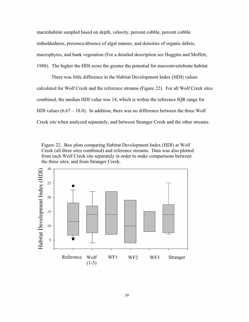
macrohabitat sampled based on depth, velocity, percent cobble, percent cobble
imbeddedness, presence/absence of algal masses, and densities of organic debris,
macrophytes, and bank vegetation (For a detailed description see Huggins and Moffett,
1988). The higher the HDI score the greater the potential for macroinvertebrate habitat.
There was little difference in the Habitat Development Index (HDI) values
calculated for Wolf Creek and the reference streams (Figure 22). For all Wolf Creek sites
combined, the median HDI value was 14, which is within the reference IQR range for
HDI values (6.67 – 18.0). In addition, there was no difference between the three Wolf
Creek site when analyzed separately, and between Stranger Creek and the other streams.
Hab
itat D
evel
opm
ent I
ndex
(HD
I)
5
10
15
20
25
30
WF1 WF2 WF3Wolf(1-3)
Reference
Figure 22. Box plots comparing Habitat Development Index (HDI) at Wolf Creek (all three sites combined) and reference streams. Data was also plotted from each Wolf Creek site separately in order to make comparisons between the three sites, and from Stranger Creek.
Stranger
39
Aquatic Invertebrates:
Several types of metrics were used to determine if macroinvertebrate communities
within Wolf Creek deviated from reference conditions. Richness metrics (total taxa and
EPT richness) allow for the analysis of community response to disturbance and are an
important indicator or macroinvertebrate community health (Huggins and Bouchard,
2000). Abundance measures (total and EPT abundance) provide an effective tool for
identifying disturbances such as nutrient loading, habitat destruction and the presence of
toxic materials. Community composition measures (%EPT) highlight the presence or
absence of pollution intolerant species and therefore are an effective indicator of
disturbance (Huggins and Bouchard, 2000).
Family Richness:
The number of macroinvertebrate taxa collected from Wolf Creek was similar to
the number of taxa collected from the streams within the reference watersheds (Table 2;
Figure 23). For example, the median value for Wolf Creek was 15 families, which was
within the IQR for reference watershed (11 – 15 families). When compared separately,
all three Wolf Creek sites had median richness values within or above (Site 2) the
reference IQR. When sampled in 2001, Stranger Creek also exhibited richness values
similar to reference conditions and Wolf Creek.
With respect to EPT richness, a similar pattern was observed (Figure 24). The
IQR range of EPT richness for the reference streams was 4 – 6 families. The median
EPT richness for the three Wolf Creek sites combined was 4.5 families. The median EPT
40
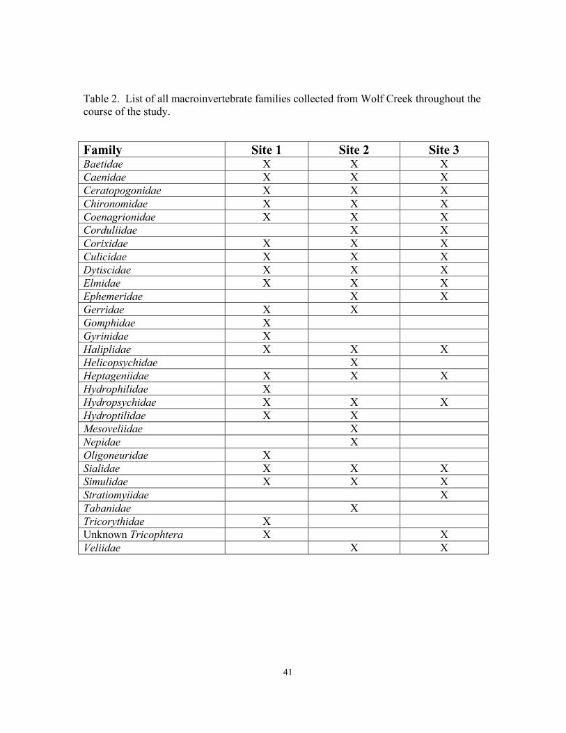
Table 2. List of all macroinvertebrate families collected from Wolf Creek throughout the course of the study.
Family Site 1 Site 2 Site 3 Baetidae X X X Caenidae X X X Ceratopogonidae X X X Chironomidae X X X Coenagrionidae X X X Corduliidae X X Corixidae X X X Culicidae X X X Dytiscidae X X X Elmidae X X X Ephemeridae X X Gerridae X X Gomphidae X Gyrinidae X Haliplidae X X X Helicopsychidae X Heptageniidae X X X Hydrophilidae X Hydropsychidae X X X Hydroptilidae X X Mesoveliidae X Nepidae X Oligoneuridae X Sialidae X X X Simulidae X X X Stratiomyiidae X Tabanidae X Tricorythidae X Unknown Tricophtera X X Veliidae X X
41
Fam
ily R
ichn
ess
0
5
10
15
20
25
WF1 WF2 WF3Wolf(1-3)
Reference
Figure 23. Box plots comparing family richness at Wolf Creek (all three sites combined) and reference streams. Data was also plotted from each Wolf Creek site separately in order to make comparisons between the three sites, and from Stranger Creek.
Stranger
EPT
Ric
hnes
s
0
5
10
WF1 WF2 WF3Wolf(1-3)
Reference
Figure 24. Box plots comparing EPT richness at Wolf Creek (all three sites combined) and reference streams. Data was also plotted from each Wolf Creek site separately in order to make comparisons between the three sites, and fromStranger Creek.
Stranger
42

richness value for Stranger Creek was also with the reference IQR, although it was at the
lower end of this range (4 families).
Abundance:
The total abundance of macroinvertebrates at Wolf Creek fell within the IQR
range for reference streams (Figure 25). The median value of macroinvertebrates
collected from the sites was 218 individuals, which was within the reference IQR range
(140 – 887 individuals). In addition, there was not a difference in the number of
individuals collected from Stranger Creek and the other sites.
Similarly, there was no difference in the abundance of EPT taxa between Wolf
Creek and the reference watersheds (Figure 26). For example, the median value for all
43
Tota
l Abu
ndan
ce
0
500
1000
1500
2000
WF1 WF2 WF3Wolf(1-3)
Reference
Figure 25. Box plots comparing insect abundance at Wolf Creek (all three sites combined) and reference streams. Data was also plotted from each Wolf Creek site separately in order to make comparisons between the three sites, and from Stranger Creek.
Stranger
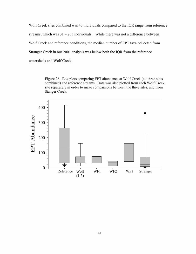
Wolf Creek sites combined was 43 individuals compared to the IQR range from reference
streams, which was 31 – 265 individuals. While there was not a difference between
Wolf Creek and reference conditions, the median number of EPT taxa collected from
Stranger Creek in our 2001 analysis was below both the IQR from the reference
watersheds and Wolf Creek.
EPT
Abu
ndan
ce
0
100
200
300
400
WF1 WF2 WF3Wolf(1-3)
Reference
Figure 26. Box plots comparing EPT abundance at Wolf Creek (all three sites combined) and reference streams. Data was also plotted from each Wolf Creek site separately in order to make comparisons between the three sites, and fromStanger Creek.
Stranger
44
% E
PT
0102030405060708090
100
WF1 WF2 WF3Wolf(1-3)
Reference
Figure 27. Box plots comparing %EPT at Wolf Creek (all three sites combined) and reference streams. Data was also plotted from each Wolf Creek site separately in order to make comparisons between the three sites, and from Stranger Creek.
Stranger
Community Composition (%EPT):
In accordance with EPT abundance, the median %EPT from Wolf Creek was
within the reference IQR for %EPT (Figure 27). For example, 27.3% of the invertebrate
community at Wolf Creek was comprised of EPT taxa and the range for reference
streams was 16.66-41.38%. In contrast to EPT abundance, the median %EPT of Stranger
Creek was greater than the reference and Wolf Creek IQR’s.
45
Conclusion: Wolf Creek
We conducted an ecological assessment of the physical, chemical, and biological
characteristics of Wolf Creek, in Leavenworth County, Kansas. We compared data
collected from three sites located along Wolf Creek during three seasons (spring,
summer, and fall) to data collected from reference watersheds that were considered to
have high habitat, water quality, and biological conditions. This analysis was used to
determine if Wolf Creek has experienced degradation, and will be used in the
development of long-term watershed management plans.
Overall, our data suggests that the ecological conditions of Wolf Creek are very
similar to the ecological conditions of the reference streams. With respect to our
analysis of stream habitat characteristics, Wolf Creek scored at least as good as reference
streams for almost all of the measured variables. For example, the median values for
riparian condition, riparian width, stream shading, and erosional area from Wolf Creek
were all within the reference IQR’s for these variables.
However, when we looked at each site separately there were indications that the
riparian forest at site 1 has experienced some level of disturbance. A large portion of the
riparian forest at this site has been removed leading to reductions in the amount of shade
available, a greater amount of erosional area, and increased channel widths. It is
important that the intact riparian forest along Wolf Creek is protected, and that there is
development of new riparian forest where it has been removed. A healthy riparian zone
will provide bank stability that reduces soil erosion and removes soil from the water as it
enters the stream leading to lower turbidity concentrations (EPA, 1996; Kalff, 2002).
46
The majority of water quality parameters that we measured in Wolf Creek were
similar to, or better then, reference conditions. For example, Wolf Creek does not appear
to be experiencing excessive nutrient loads from its watershed. Wolf Creek exhibited
both total nitrogen and phosphorus values that were lower (better) than reference streams.
However, there were two water quality variables that scored poorer than reference
streams and were close to the lower limits of the current Kansas surface water standards.
These variables include turbidity, which was higher than in reference streams and
dissolved oxygen, which was lower than in reference streams. While both of these
variables can have significant negative impacts on the biological communities within a
stream, our analysis of both macroinvertebrate and fish communities suggest that the
biological communities of Wolf Creek are at least as healthy as the communities in the
reference streams. It is possible that increased turbidity and low dissolved oxygen levels
may negatively impact these communities in the future, and additional long-term
monitoring is warranted at Wolf Creek.
We also included several biotic components of Wolf Creek in our analysis.
Although we were unable to compare periphyton collected from Wolf Creek with the
reference streams, we were able to compare data from Wolf Creek with similar data
collected from Stranger Creek in 2001 (Liechti and Dzialowski, 2002). Benthic algal
concentrations (i.e. chlorophyll a) did not differ between the three Wolf Creek sites.
However, algal concentrations at Wolf Creek were lower than at Stranger Creek, further
supporting our findings that Wolf Creek is not experiencing high nutrient loads.
Analysis of the macroinvertebrate and fish data collected at each site suggests that
Wolf Creek has not deviated from reference conditions. The median values for all of the
47

metrics used to assess these biotic communities at Wolf Creek were within, or greater
than, the range of values obtained for reference streams. Therefore, these communities
are diverse and represented by a number of indicator species (i.e EPT). We believe that
this data suggests that the macroinvertebrate and fish communities at Wolf Creek are
currently healthy. We recommend that further sampling be conducted in order to monitor
any changes in these communities that may occur from future disturbances within the
watershed.
Based on the overall analysis of the ecological conditions at Wolf Creek, it
appears this system is relatively healthy. There is some concern of riparian loss (site 1),
high turbidity levels, and low dissolved oxygen levels within Wolf Creek. However,
biotic communities do not appear to be negatively affected at this time. For example,
Wolf Creek does not appear to be experiencing excessive algal blooms, and both
macroinvertebrate and fish communities are at least as diverse as reference in streams.
Land use management and the preservation and improvement of instream habitat, in
combination with continued monitoring will help to maintain the overall health of the
Wolf Creek watershed.
48

Stranger Creek: Background
The KBS previously conducted an ecological assessment of Stranger Creek
(Liechti and Dzialowski, 2002). Using methodology similar to that used in the
assessment of Wolf Creek, we sampled three sites along the main stem of Stranger Creek
during three separate sampling events in 2001. Based on this original 2001 analysis, we
found that there was a high degree of site variability at Stranger Creek. For example, the
inorganic substrate at sites 1 and 3 was very diverse and dominated by several substrate
types including cobble, soft silt, hard clay, and sand. In contrast, site 2 was much less
diverse and dominated by soft silt. Similarly, site 2 scored lower than the other two sites
on most variables measuring the health of the riparian forest (Liechti and Dzialowski,
2001).
Since in-stream and near-stream variables are directly related to the health and
diversity of the resulting fish communities (Allen, 1995), we were interested in
determining if the conditions at sites 1 and 3, or the conditions at site 2 were more
representative of the overall conditions and available habitat at Stranger Creek. Based on
the placement of our original sampling sites, there is reason to believe that the overall
ecological conditions of Stranger Creek are more similar to site 2. For example, while
sites 1 and 3 had high fish habitat potential, they were also located directly below
bridges, which provided non-natural habitat.
In our initial assessment of Stranger Creek we stated, “it is likely that the level of
impairment at Stranger Creek is related to the proportion of the total stream area that is
similar to each of the three sites. For example, if a large proportion of Stranger Creek has
ecological conditions similar to those found at ST2, then the ecological integrity of
49

Stranger Creek has likely been severely compromised” (Liechti and Dzialowski, 2002).
Therefore, we sampled several additional sites along Stranger Creek in November of
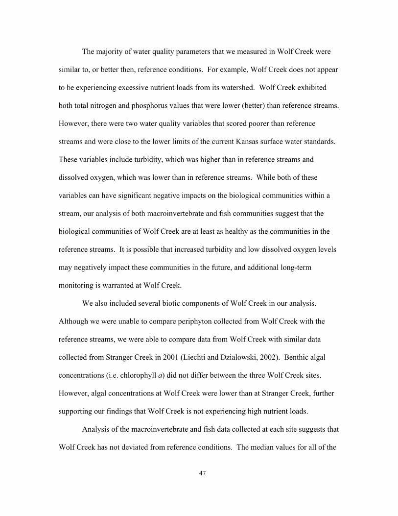
2003 in order re-asses the availability of potential fish habitat. Five new sites were
selected for this analysis (Figure 28). One site was selected 100 m above our original site
1 and another site was selected 100 m above our original site 3 in order to determine the
conditions outside the zone of influence associated with the bridges in these areas. Three
additional sites were selected that were not directly affected by bridges, and that had
relatively good riparian forests (51 – 75% of desired corridor available) as determined by
the “Stranger Creek Watershed Management Plan” (Leavenworth County Planning
Department, 2002). At each site a number of instream variables associated with fish
habitat including inorganic substrate, areas of undercutting, areas of vegetative cover, and
stream shading were measured using methodology described above for Wolf Creek.
Stranger Creek Results: Habitat measurements
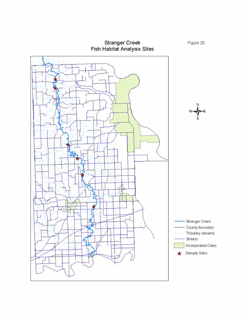
The available inorganic habitat at the five Stranger Creek sites was dominated by
soft silt (Figure 29). In addition, gravel (11%), hard clay (6%), and sand (3%) were
present, but only in small quantities. Cobble, which is often considered to be an
important habitat type for both fish and macroinvertebrates (Allen, 1985), was not present
at any of the Stranger Creek sites sampled in 2003. In comparison with our previous
analysis of the inorganic substrate availability at Stranger Creek (Liechti and Dzialowski,
2002), this data suggests that substrate conditions at our original site 2 are likely more
representative of the overall conditions at Stranger Creek (Figure 30). For example, we
found that soft silt comprised only 17 and 16% of the available substrate at Stranger
50
51
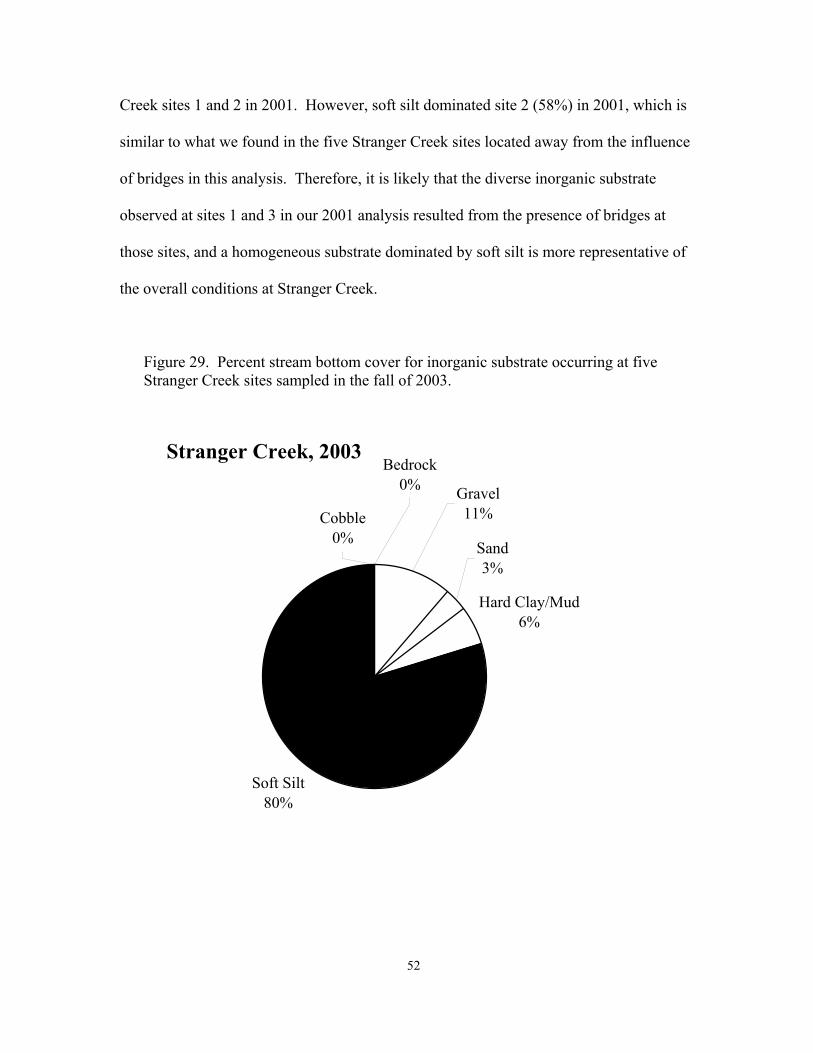
Creek sites 1 and 2 in 2001. However, soft silt dominated site 2 (58%) in 2001, which is
similar to what we found in the five Stranger Creek sites located away from the influence
of bridges in this analysis. Therefore, it is likely that the diverse inorganic substrate
observed at sites 1 and 3 in our 2001 analysis resulted from the presence of bridges at
those sites, and a homogeneous substrate dominated by soft silt is more representative of
the overall conditions at Stranger Creek.
Figure 29. Percent stream bottom cover for inorganic substrate occurring at five Stranger Creek sites sampled in the fall of 2003.
Stranger Creek, 2003
Hard Clay/Mud6%
Soft Silt80%
Cobble0%
Bedrock0%
Sand3%
Gravel11%
52
Figure 30. Percent stream bottom cover for inorganic substrate occurring at the three Stranger Creek sites in 2001 (Liechti and Dzialowski, 2002).
ST1
Bedrock16%
Cobble38%
Gravel1%
Sand11%
Hard Clay/Mud
17%
Soft Silt17%
53
ST2
Soft Silt58%
Hard Clay/Mud
29%
Sand10%
Gravel3%
ST3Bedrock
2%Cobble
29%
Gravel4%
Sand18%
Hard Clay/Mud31%
Soft Silt16%
We did find areas of bank undercutting and vegetative overhang at several of the
Stranger Creek sites sampled in 2003. While these variables represent potential fish
habitat, only small areas were present. Furthermore, no major differences existed
between the data collected in 2001 and 2003. For example, the median amount of bank
undercutting found at the three original Stranger Creek sites sampled in 2001 was 0.70
m3, compared to 0.99 m3 at the five Stranger Creek sites sampled in 2003.
Stre
am S
hadi
ng (%
)
0
10
20
30
40
50
60
ST1(2001)
ST2(2001)
ST3(2001)
Stranger(2003)
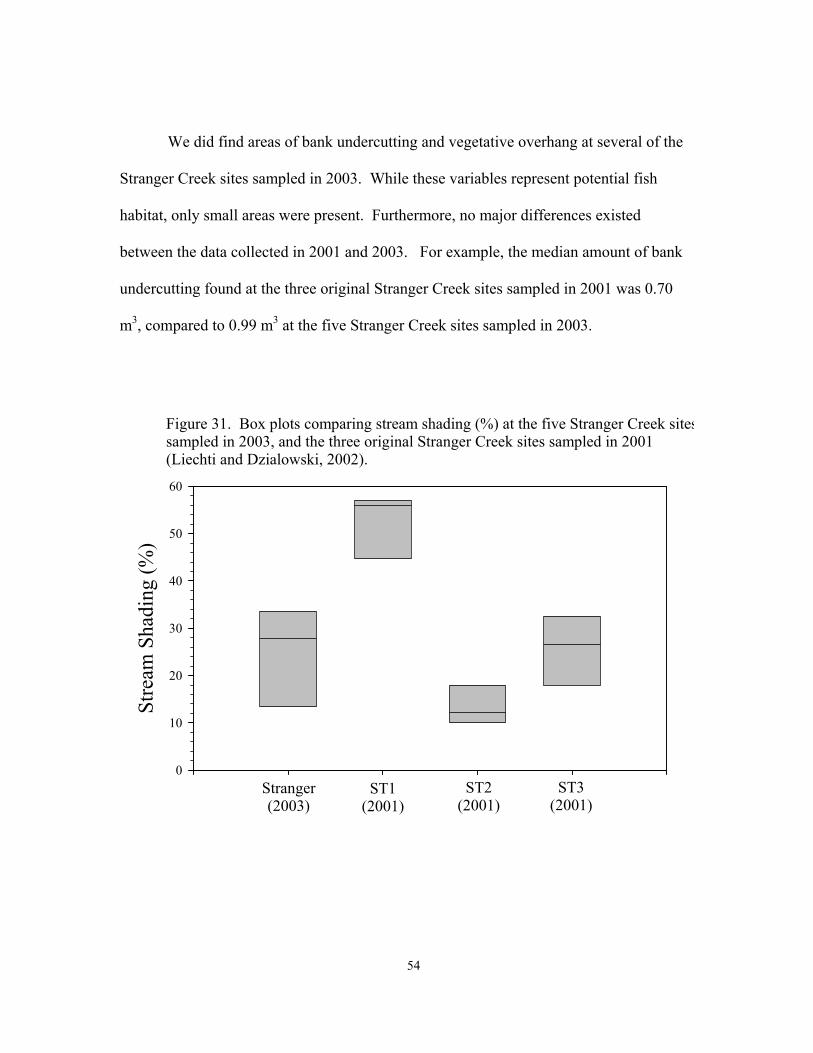
Figure 31. Box plots comparing stream shading (%) at the five Stranger Creek sitessampled in 2003, and the three original Stranger Creek sites sampled in 2001 (Liechti and Dzialowski, 2002).
54

We also measured the percent stream shading from the canopy cover at each site.
Stream shading is directly related to water temperature, and the distribution of many fish
species is limited by temperature. The median % stream shading for the five sites
sampled in 2003 was 27.94% (Figure 31). This median value was similar to the median
value observed at site 3 in 2001, but much lower than the median value observed for site
1 in 2001. These results suggest that % stream shading at Stranger Creek is similar to the
results that we observed for sites 2 and 3 in 2001.
Conclusions: Stranger Creek
We sampled several sites along Stranger Creek in order to assess the available
fish habitat. Based on our initial analysis in 2001 (Liechti and Dzialowski, 2001), it was
unknown if the high habitat measures that were observed were the result of several sites
being located near bridges. By looking at an additional five sites, all of which were out
of the influence of bridges, we were able to assess the habitat and determine if it has been
severely degraded.
We found that the inorganic substrate composition at the five Stranger Creek sites
sampled in 2003 was very similar to the substrate composition at site 2, which was the
only site in our initial analysis not located near a bridge. The substrate composition at
site 2 was homogeneous and dominated by soft silt, which is indicative of high flow
conditions, high erosion, and high levels of siltation within the watershed. Based on this
analysis, we suggest that the overall fish habitat at Stranger Creek has been severely
compromised and that the ecological conditions of site 2 as described in our initial
assessment more accurately represent the fish habitat conditions at Stranger Creek.
55
Moreover, at the 3 sites located where there was relatively good riparian forest,
fish habitat did not appear to be any better than at other sites where measurement were
taken. The deeply incised stream channel through out the length of Stranger Creek, the
consequence of altered hydrology and a thick mantel of highly erodible loess soils, may
have compromised the beneficial effects of a good, intact riparian corridor along the
stream banks. Future efforts to reestablish riparian vegetation along Stranger Creek may
also require concurrent actions to restore a more natural hydrology to realize an
improvement in the habitat available for fish in Stranger Creek.
56
References
Allan, J.D. 1995. Stream Ecology: Structure and function of running waters. 388pp. Chapman & Hall, New York.
Barbour, M.T., J. Gerritsen, B.D. Snyder, and J.B. Stribling. 1999. Rapid bioassessment
protocols for use in streams and wadeable rivers: periphyton, benthic macroinvertebrates, and fish, Second Edition. EPA 841-B-99-002. U.S. Environmental Protection Agency; Office of Water; Washington, D.C.
Berkman, H.E., C.F. Rabeni, and T.P. Boyle. 1986. Biomonitors of stream quality in
agricultural areas: fish versus invertebrates. Environmental Management 10(3):413-419.
Cross. F., and J. Collins. 1995. Fishes in Kansas. Public Ed. Series #14, University of
Kansas, Lawrence, 315pp. deNoyelles, J.D, W.D. Kettle, and D.E. Sinn. 1982. The responses of plankton
communities in experimental ponds to atrazine, the most heavily used pesticide in the United States. Ecology 63:1285-1293.
Huggins, D.G., and M. Moffett. 1988. A proposed biotic index and habitat development
index for use in Streams in Kansas. Report #35 of the Kansas Biological Survey, Lawrence, KS. 128 pp.
Huggins, D.G., and R.W. Bouchard. 2000. Aquatic habitat and biology module for the
Big Soldier Creek watershed management plan. Report of the Kansas Biological Survey, Lawrence, KS. 111pp.
Hughes, R.M., D.P. Larsen, and J. Omernik. 1986, Regional reference sites: a method for
assessing stream potentials. Environmental Management 10:629-635. Kalff, J. 2002. Limnology. 592pp. Prentice-Hall, New Jersey. Karr, J., K. Fausch, P. Angermeier, P. Yant, and I. Schlosser. 1986. Assessing biological
integrity of running waters: a method and its rational. Sp. Publ. 5, I. Natural Hist. Surv., Urbane, IL.
Leavenworth County Comprehensive Plan 2020. Chapter 9A. Stanger Creek Watershed
Management Plan. Leavenworth County Planning Department, Laevenworth, Kansas.
Liechti, P., and A.R. Dzialowski. 2002. Final assessment of the ecological integrity of
Stranger Creek (Leavenworth County, Kansas). Final report submitted to Leavenworth County, 47 pp.
57

Miller, D., L. Leonard, R. Hughes, J. Karr, P.Moyle, L. Schrader, B. Thompson, R.
Daniels, K. Fausch, G. Fitzhugh, J. Gammon, D. Halliwell, P. Angermeier, and D. Orth. 1988. Regional applications of an index of biotic integrity for use in water resource management. Fisheries 13(5):12-20.
Platts, W.S., C. Armour, G.D. Booth, M. Bryant, J.L. Buford, P. Cuplin, S. Jensen, G.W.
Minshall, S.B. Morsen, R.L. Nelson, J.R. Sedell, and J.S. Tuhy. 1987. Methods for evaluating riparian habitats with application to management. USDA, Forest Service, General Technical Report, I NT-221:1-177.
Rosenberg, D.M. and V.H. Resh. 1996. Use of aquatic insects in biomonitoring. In
Aquatic Insects of North America, R. Merritt and K. Cummins (eds.). Kendall/Hunt Publ., Dubuque, Iowa.
Smith, V.H. 2003. Eutrophication of freshwater and coastal marine ecosystems: A global
problem. Environmental Science and Pollution Research 10:1-11. Trombley, T.J. 2001. Quality of water on the Prairie Band Potawatoma Reservation,
northeastern Kansas, February 199 through February 2001: U.S. Geological Survey Water-Resources Investigations Report 01-4196.
USEPA (Environmental Protection Agency). 1996. Biological criteria: technical
guidance for streams and rivers (revised) EPA 822-B-96-001. U.S. Environ. Protect. Agen., Office of Water, Washington, D.C. 162pp.
Washington, H.G. 1984. Diversity, biotic and similarity indices: A review with special
relevance to aquatic ecosystems. Water Resources 18:653-694. Whiles, M.R., B.L. Brock, A.C. Franzen, and S.C. Dinsmore. 2000. Stream invertebrate
communities, water quality, and land-use patterns in an agricultural drainage basin of northeastern Nebraska, USA. Environmental Management 26(5):563-576.
58