Embed Size (px)
Citation preview


J. Software Engineering & Applications, 2010, 3 Published Online January 2010 in SciRes(www.SciRP.org/journal/jsea)
Copyright © 2010 SciRes JSEA
CONTENTS
Volume 3 Number 1 January 2010 Models for Improving Software System Size Estimates during Development
W. W. AGRESTI, W. M. EVANCO & W. M. THOMAS………………………………………………1
A Massively Parallel Re-Configurable Mesh Computer Emulator: Design, Modeling and Realization
M. YOUSSFI, O. BOUATTANE & M. O. BENSALAH………………………………………………11
Properties of Nash Equilibrium Retail Prices in Contract Model with a Supplier, Multiple Retailers and Price-Dependent Demand
K. NAKADE, S. TSUBOUCHI & I. SEDIRI……………………………………………………………27
A Polar Coordinate System Based Grid Algorithm for Star Identification
H. ZHANG, H. S. SANG & X. B. SHEN………………………………………………………………34
Evaluation of Feature Subset Selection, Feature Weighting, and Prototype Selection for Biomedical Applications
S. LITTLE, S. COLANTONIO, O. SALVETTI & P. PERNER…………………………………………39
Cryptanalysis of TEA Using Quantum-Inspired Genetic Algorithms
W. HU……………………………………………………………………………………………………50
Application of Design Patterns in Process of Large-Scale Software Evolving
W. WANG, H. ZHAO, H. LI, P. Li, D. YAO, Z. LIU, B. LI, S. YU, H. LIU & K. Z. YANG…………58
Element Retrieval Using Namespace Based on Keyword Search over XML Documents
Y. WANG, Z. K. CHEN & X. D. HUANG………………………………………………………………65
Integrated Web Architecture Based on Web3D, Flex and SSH
W. J. ZHANG……………………………………………………………………………………………73
Analysis and Comparison of Five Kinds of Typical Device-Level Embedded Operating Systems
J. L. WANG, H. ZHAO, P. LI, H. LI & B. LI……………………………………………………………81
Makespan Algorithms and Heuristic for Internet-Based Collaborative Manufacturing Process Using Bottleneck Approach
S. A. BAREDUAN & S. HASAN………………………………………………………………………91

Journal of Software Engineering and Applications (JSEA)
Journal Information
SUBSCRIPTIONS
The Journal of Software Engineering and Applications (Online at Scientific Research Publishing, www.SciRP.org)
is published monthly by Scientific Research Publishing, Inc., USA.
E-mail: [email protected]
Subscription rates: Volume 3 2010 Print: $50 per copy.
Electronic: free, available on www.SciRP.org.
To subscribe, please contact Journals Subscriptions Department, E-mail: [email protected]
Sample copies: If you are interested in subscribing, you may obtain a free sample copy by contacting Scientific
Research Publishing, Inc. at the above address.
SERVICES
Advertisements
Advertisement Sales Department, E-mail: [email protected]
Reprints (minimum quantity 100 copies)
Reprints Co-ordinator, Scientific Research Publishing, Inc., USA.
E-mail: [email protected]
COPYRIGHT
Copyright© 2010 Scientific Research Publishing, Inc.
All Rights Reserved. No part of this publication may be reproduced, stored in a retrieval system, or transmitted, in
any form or by any means, electronic, mechanical, photocopying, recording, scanning or otherwise, except as
described below, without the permission in writing of the Publisher.
Copying of articles is not permitted except for personal and internal use, to the extent permitted by national
copyright law, or under the terms of a license issued by the national Reproduction Rights Organization.
Requests for permission for other kinds of copying, such as copying for general distribution, for advertising or
promotional purposes, for creating new collective works or for resale, and other enquiries should be addressed to
the Publisher.
Statements and opinions expressed in the articles and communications are those of the individual contributors and
not the statements and opinion of Scientific Research Publishing, Inc. We assume no responsibility or liability for
any damage or injury to persons or property arising out of the use of any materials, instructions, methods or ideas
contained herein. We expressly disclaim any implied warranties of merchantability or fitness for a particular
purpose. If expert assistance is required, the services of a competent professional person should be sought.
PRODUCTION INFORMATION
For manuscripts that have been accepted for publication, please contact:
E-mail: [email protected]
J. Software Engineering & Applications, 2010, 3: 1-10 doi:10.4236/jsea.2010.31001 Published Online January 2010 (http://www.SciRP.org/journal/jsea)
Copyright © 2010 SciRes JSEA
1
Models for Improving Software System Size Estimates during Development
William W. AGRESTI1, William M. EVANCO2, William M. THOMAS3
1Carey Business School, Johns Hopkins University, Baltimore, USA; 2Statistical Solutions, Philadelphia, USA; 3The MITRE Corpo-ration, McLean, VA, USA. Email: [email protected], [email protected], [email protected] Received August 28th, 2009; revised September 16th, 2009; accepted September 29th, 2009.
ABSTRACT
This paper addresses the challenge of estimating eventual software system size during a development project. The ap-proach is to build a family of estimation models that use information about architectural design characteristics of the evolving software product as leading indicators of system size. Four models were developed to provide an increasingly accurate size estimate throughout the design process. Multivariate regression analyses were conducted using 21 Ada subsystems, totaling 183,000 lines of code. The models explain from 47% of the variation in delivered software size early in the design phase, to 89% late in the design phase. Keywords: Software Size, Estimation, Ada, Regression, Re-Estimation, Metrics
1. Introduction
Before software development projects start, customers and managers want to know the eventual project cost with as much accuracy as possible. Cost estimation is extremely important to provide an early indicator of what lies ahead: will the budget be sufficient for this job? This need has motivated the development of software cost estimation models, and the growth of a commercial market for such models, associated automated tools, and consulting sup-port services.
When someone who is new to the use of cost estima-tion models looks at the estimation equation, it can be quite disconcerting. The only recognizable variable on the right-hand side is size, surrounded by a few modify-ing factors and shape parameters. So, if the project is just beginning, how do you know the size of the system? More experienced staff members explain that you must first estimate the size so that you can supply that value in the equation, thus enabling you to estimate cost. How good can the cost estimate be if it depends so strongly on a quantity that won’t be known until the end of the pro-ject? The underlying logic prompting this question is irrefutable. This situation is well known and recognized (e.g., [1, 2]). Users of such cost estimation models are dependent, first and foremost, on accurate size estimates. Of course, there are other ways to estimate costs (e.g., by analogy and experience), but the more analytically satis-fying models estimate cost as a function of size. Thus,
the need for an accurate cost estimate often translates into a need for an accurate size estimate.
This paper addresses size estimation, but distinguishes between estimation before development and during de-velopment. Size estimation prior to the start of a software project typically draws on analogy and professional judgment, with comparisons of the proposed system to previously developed systems of related functionality. Function point counts may also be used to provide an estimate of size, but, of course, the accuracy of the size estimate depends on accurate knowledge of the entities being counted.
Once the project begins, managers would like to keep improving their size estimate. However, we are moti-vated by our observations of current practice in which managers, during development, revert to predevelopment estimates of size (and effort and cost) because of a lack of effective ways to incorporate current development information to refine their initial estimates [3]. Ideally there would be straightforward methods to improve the predevelopment estimates based on early project experi-ences and the evolving product. In this paper we focus on the evolving product as a source of information for up-dating the size estimate.
The research reported in this paper addresses the ques-tion of how to improve our capability for estimating the size of software systems during a development project. More specifically, it reports on building a family of models for successively refining the size estimate during
Models for Improving Software System Size Estimates during Development 2
the development process. The notion of a family of mod-els is intended to address the challenge of successively refining the initial estimate as the project unfolds. The research has three motivations: the widely known poor record of large software projects to be delivered on time and on budget (due in part to poor estimation capability), the persistent illogic of needing to know size to estimate cost, and the challenge of successive size reestimation during a project.
The remainder of the paper discusses related work, the design and implementation process, the estimation mod-els, the empirical study, statistical results, limitations of the analyses, and future directions.
2. Related Work
Reasonably accurate size estimates may be achievable when an organization has experience building systems in the domain of the new project. The new system may be analogous to previous ones or related to a product line that is familiar. There may even be significant reuse of class libraries, designs, interfaces, or code to make the estimation easier. But accurately estimating eventual system size grows more difficult when the new system ranks higher in novelty or, using the nomenclature of systems engineering, is unprecedented. Even when the application domains are similar, new projects may re-quire significantly more code to account for enhanced requirements for security and robustness that were not associated with previous systems.
An especially appealing category of estimation models is one that consists of models that use early constructs from the evolving system. The analyses that are closest to the research reported here were done as part of the evolution of COCOMO models over the years. CO-COMO II has the characteristic of the models being built in this paper by recognizing the need for a family of models. For COCOMO II, the models take advantage of increased learning during the project: the early prototyp-ing stage, early design stage, and postarchitecture stage [4].
As development gets underway in a project, the repre-sentations used in specification and design provide op-portunities for the measurement of key constructs used in those representations. Then models can be built to relate values from those constructs to measures of system size. This practice has been in place for decades. One of the earliest and most influential of such models was Tom DeMarco’s Bang metric that related values from data flow diagrams and other notations to eventual code size. [5]. Similar models have been built, based on capturing measures of entity-relationship and state-transition dia-grams from early system specifications [6]. Bourque and Cote [7] performed an experiment to develop and vali-date such a predictive model based on specification measures that were obtained from data flow and entity-
relationship diagrams. It was found that a model using the number of data elements crossing an elementary pro- cess in the data flow diagram as the sole explanatory variable performed fairly well as a predictive model.
Much of the research using early system artifacts for estimation is directed at estimating effort and cost. Pau- lish, et al., discussed the use of the software architecture document as the primary input to project planning [8]. Mohagheghi et al., described an effort estimation model based on the actual use cases of the system being built [9]. Pfleeger used a count of objects and methods as a size measure in a model of software effort [10]. Jensen and Bartley investigated the use of object information obtained from specifications in models of programmer effort [11]. They proposed that development effort is a function of the number of objects, operations, and inter-faces in the system, and that counts of these entities can be obtained from a textual specification.
More closely related to the current paper is reported research that is focused on estimating size. Laranjeira [12] provided a method for sizing object-oriented systems based on successive estimations of refinements of the system objects. As the system becomes more refined, a greater confidence in the size estimates is obtained. He proposed the use of statistical techniques to determine a rate of convergence to the actual estimate. The estimation is still subjective, but the method gives an indication of progress toward the convergence of the estimates, and as such provides an objective, statistically based confidence interval for the estimates.
Minkiewicz [13] offers a useful overview of the evolu-tion and value of various measures of size, including the most widely used, lines of code and function points. The model in [14] estimated size, as measured by function points [15] directly from a conceptual model of the sys-tem being built. Tan et al. built a model to estimate lines of code based on the counts of entities, relationships, and attributes from the conceptual data model [16]. A model by Diev [17] related early information on use cases into a size estimate, measured in function points. The models in [18] produce lines-of-code estimated from a VHDL-based design description. Antoniol et al. investi-gated the adapting of function points to object-oriented systems by defining object-oriented function points (OO FPs) [1]. They first identified constructs in object- ori-ented systems (e.g., classes and methods) to use as pa-rameters for OOFPs, then built a flexible model to esti-mate system size. Their pilot study showed that the model was promising as a way to estimate lines of code from OOFPs.
There has been considerable research on ways to use object-oriented designs in the Unified Modeling Lan-guage (UML) to estimate size as measured in function points. Capturing the design in UML facilitates develop-ing an automated tool to extract counts of entities and
Copyright © 2010 SciRes JSEA
Models for Improving Software System Size Estimates during Development
Copyright © 2010 SciRes JSEA
3
other data that can be used in empirical studies to de-velop size estimation models. Most similar to the re-search here are studies that developed families of models that provided a succession of estimates as more design information is known. For example, Zivkovic et al. [19] developed automated approaches to estimating function point size using UML design information, including data types and transactional types. Hericko and Zivkovic’s analysis [20] was most similar to the research reported here because it involved basing the size estimate on more detailed information about a UML design. The first esti-mate used use case diagrams, the second estimate added information from activity diagrams, and the final esti-mate added information from class diagrams. The esti-mates, which did improve as new information was in-corporated into the models, produced an estimate meas-ured in function points, as opposed to the lines of code used in the research in this paper.
3. The Design and Implementation Process
Our analysis and model building relies on assumptions concerning the progress of design and implementation. This section discusses these assumptions.
We are investigating systems that were built in Ada, which proceeds from specifying relationships among larger units (packages) to a specification of the interior details of these units. Ada was used as a design notation, which means that a machine-readable design artifact is available for observation and analysis. Royce [21] was one of the first to discuss this use of a single language in the Ada process model: “Regardless of level, the activity being performed is Ada coding. Top-level design means
coding the top-level components (Ada main programs, task executives, global types, global objects, top-level library units, etc.). Lower-level design means coding the lower-level program unit specifications and bodies.”
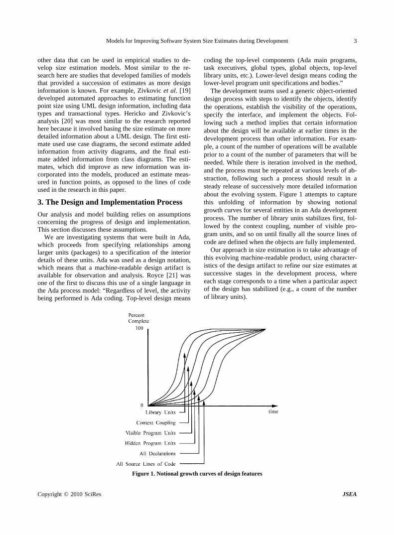
The development teams used a generic object-oriented design process with steps to identify the objects, identify the operations, establish the visibility of the operations, specify the interface, and implement the objects. Fol-lowing such a method implies that certain information about the design will be available at earlier times in the development process than other information. For exam-ple, a count of the number of operations will be available prior to a count of the number of parameters that will be needed. While there is iteration involved in the method, and the process must be repeated at various levels of ab-straction, following such a process should result in a steady release of successively more detailed information about the evolving system. Figure 1 attempts to capture this unfolding of information by showing notional growth curves for several entities in an Ada development process. The number of library units stabilizes first, fol-lowed by the context coupling, number of visible pro-gram units, and so on until finally all the source lines of code are defined when the objects are fully implemented.
Our approach in size estimation is to take advantage of this evolving machine-readable product, using character-istics of the design artifact to refine our size estimates at successive stages in the development process, where each stage corresponds to a time when a particular aspect of the design has stabilized (e.g., a count of the number of library units).
Figure 1. Notional growth curves of design features
Models for Improving Software System Size Estimates during Development 4
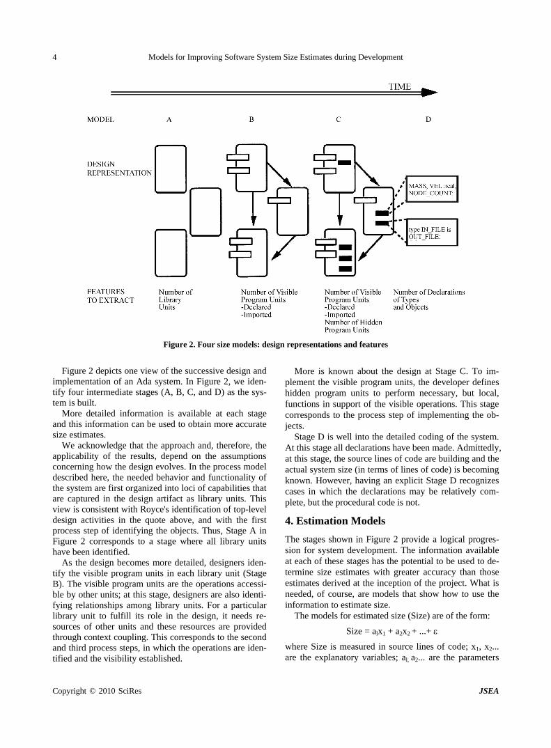
Figure 2. Four size models: design representations and features
Figure 2 depicts one view of the successive design and
implementation of an Ada system. In Figure 2, we iden-tify four intermediate stages (A, B, C, and D) as the sys-tem is built.
More detailed information is available at each stage and this information can be used to obtain more accurate size estimates.
We acknowledge that the approach and, therefore, the applicability of the results, depend on the assumptions concerning how the design evolves. In the process model described here, the needed behavior and functionality of the system are first organized into loci of capabilities that are captured in the design artifact as library units. This view is consistent with Royce's identification of top-level design activities in the quote above, and with the first process step of identifying the objects. Thus, Stage A in Figure 2 corresponds to a stage where all library units have been identified.
As the design becomes more detailed, designers iden-tify the visible program units in each library unit (Stage B). The visible program units are the operations accessi-ble by other units; at this stage, designers are also identi-fying relationships among library units. For a particular library unit to fulfill its role in the design, it needs re-sources of other units and these resources are provided through context coupling. This corresponds to the second and third process steps, in which the operations are iden-tified and the visibility established.
More is known about the design at Stage C. To im-plement the visible program units, the developer defines hidden program units to perform necessary, but local, functions in support of the visible operations. This stage corresponds to the process step of implementing the ob-jects.
Stage D is well into the detailed coding of the system. At this stage all declarations have been made. Admittedly, at this stage, the source lines of code are building and the actual system size (in terms of lines of code) is becoming known. However, having an explicit Stage D recognizes cases in which the declarations may be relatively com-plete, but the procedural code is not.
4. Estimation Models
The stages shown in Figure 2 provide a logical progres-sion for system development. The information available at each of these stages has the potential to be used to de-termine size estimates with greater accuracy than those estimates derived at the inception of the project. What is needed, of course, are models that show how to use the information to estimate size.
The models for estimated size (Size) are of the form:
Size = alx1 + a2x2 + ...+
where Size is measured in source lines of code; x1, x2... are the explanatory variables; al, a2... are the parameters
Copyright © 2010 SciRes JSEA

Models for Improving Software System Size Estimates during Development 5
to be estimated; and is an error term. Four different models were built, corresponding to the
four different stages in the design phase as shown in Fig-ure 2. These models show source lines of code estimated from ----
• Model A: the number of library units. • Model B: the number of visible and imported pro-
gram units declared. • Model C: the number of visible, imported, and hid-
den program units declared. • Model D: the number of types and objects declared. At Stage A in Figure 2, the number of library units de-
fined serves as an early indicator of system size. The size model at this stage is a coefficient multiplied by the num- ber of user defined library units in the system. Thus, the model for estimating source lines of code is:
SizeA = al * (#of library units) +
Stage B is further into the design process and more is known about the details of the library units that were the basis for the estimation at Stage A. So, at Stage B, the number of visible program units declared and program units imported from other subsystems by library units through the context coupling mechanism are the parame-ters of the size model. The rationale is that the number of visible program units is a proxy for the functionality of a package. Statistically we expect that more program units will translate into a need for more lines of Ada code. The rationale for the number of imported program units is that they are being imported because they are needed, so they must enter into the code of the receiving library unit. So, if there are more imports, statistically we expect that there will be more lines of code required in the library unit. Thus, the model appears as:
SizeB = al * (# of visible program units)
+ a2 * (# of imported program units) +
At Stage C, the size estimation model depends on the same information as Stage B, but with the inclusion of the number of hidden program units. Again, hidden pro-gram units perform local processing needed to support the visible program units. The model is of the form:
SizeC = al * (# of visible program units) + a2 * (# of imported program units) + a3 * (# of hidden program units) +
As the design progresses, more detailed declarations become available. The size estimation model at stage D uses the number of declarations of types and objects as the basis for its estimate of system size. This model ap-pears as:
SizeD = al * (# of type/subtype declarations + #object declarations) +
5. Empirical Study
To estimate the parameters of the models, we analyzed a collection of 21 Ada subsystems, from four projects de-veloped at the Software Engineering Laboratory of the National Aeronautics and Space Administration/Goddard Space Flight Center [22]. The analysis was restricted to subsystems containing more than one Ada library unit, and consisting of at least 1,000 source lines of code. The subsystems in our data set ranged in size from 2,000 to 27,000 source lines of code, excluding comment and blank lines.
A locally developed Ada source analyzer program was used [23], although other static analysis tools could yield the same data. We extracted counts of source lines of code; library units; visible, imported, and hidden pro-gram units; and type and object declarations from the delivered product. These counts were used in regression analyses to develop models of delivered product source lines of code.
Because the explanatory variables were taken from completed project code data, we cannot make claims as to whether all of the entities (library units, visible pro-gram units declared and imported, hidden program units, and declarations) were defined at stages A, B, C, and D in strict adherence to the process model. For example, while the model for Stage B depends on the number of visible program units, and the process model calls for defining the visible program units at that stage in the process, it may be that some number of additional visible program units were added very late in the process (e.g., due to a requirements change). However, the process model does provide for successive elaboration of the design and code in a seamless way with Ada as both a design and implementation language. For example, one of the authors (WA) was technical manager of one pro-ject using this process model and had over 35,000 lines of compiled Ada at the time of Critical Design Review. That is, the compiled Ada was essentially the design structure of the system, and, because it was in Ada, it was amenable to automated analysis. If a size reestima-tion model like this is used in practice, the model could be calibrated and validated on an ongoing basis during projects, so that the model is based on the actual number of visible program units defined at Stage B.
6. Statistical Results
Size estimates can be made throughout the design phase based on information with increasing detail. Because of the additional information, we would expect these esti-mates to be more accurate as the project moves into the later design phases. In terms of the statistical analyses, a greater fraction of the variation in lines of code (as
Copyright © 2010 SciRes JSEA
Models for Improving Software System Size Estimates during Development
Copyright © 2010 SciRes JSEA
6
measured by the coefficient of determination of a regres-sion analysis) would be explained as the design phase progresses. In this section we present the results of re-gression analyses of size estimation models.
As discussed previously, these models progress through greater levels of information availability as the design progresses, and they can be used to update the size esti-mates for the purposes of project management. Regres-sion analysis was used to build the models, with the ex-pected outcome that the size estimates will become more accurate as more design information becomes available.
The regressions for all four models were linear in both the source lines of code and the explanatory variables. A zero intercept term was assumed since zero values for the explanatory variables used to explain the source lines of code would necessarily imply that no lines of code would be generated. Unpublished results of regression analyses for models with the intercept terms resulted in intercept estimates that were not significantly different from zero, a conclusion also reached by Antoniol [1].
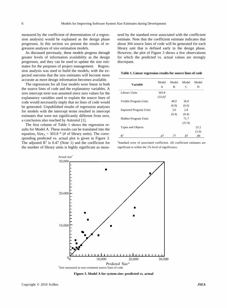
The first column of Table 1 shows the regression re-sults for Model A. These results can be translated into the equation, SizeA = 303.8 * (# of library units). The corre-sponding predicted vs. actual plot is given in Figure 3. The adjusted R2 is 0.47 (Note 1) and the coefficient for the number of library units is highly significant as meas-
ured by the standard error associated with the coefficient estimate. Note that the coefficient estimate indicates that about 304 source lines of code will be generated for each library unit that is defined early in the design phase. However, the plot of Figure 3 shows a few observations for which the predicted vs. actual values are strongly discrepant.
Table 1. Linear regression results for source lines of code
Variable Model
A
Model
B
Model
C
Model
D
Library Units 303.8
(33.6)a
Visible Program Units 48.0 36.8
(6.9) (6.6)
Imported Program Units 3.0 2.8
(0.4) (0.4)
Hidden Program Units 71.7
(21.9)
Types and Objects 22.2
(1.0)
R2 .47 .77 .87 .89
aStandard error of associated coefficient. All coefficient estimates are
significant to within the 1% level of significance.
Actual size*
*Size measured as non-comment source lines of code
Figure 3. Model A for system size: predicted vs. actual
Models for Improving Software System Size Estimates during Development 7
Actual size*
*Size measured as non-comment source lines of code
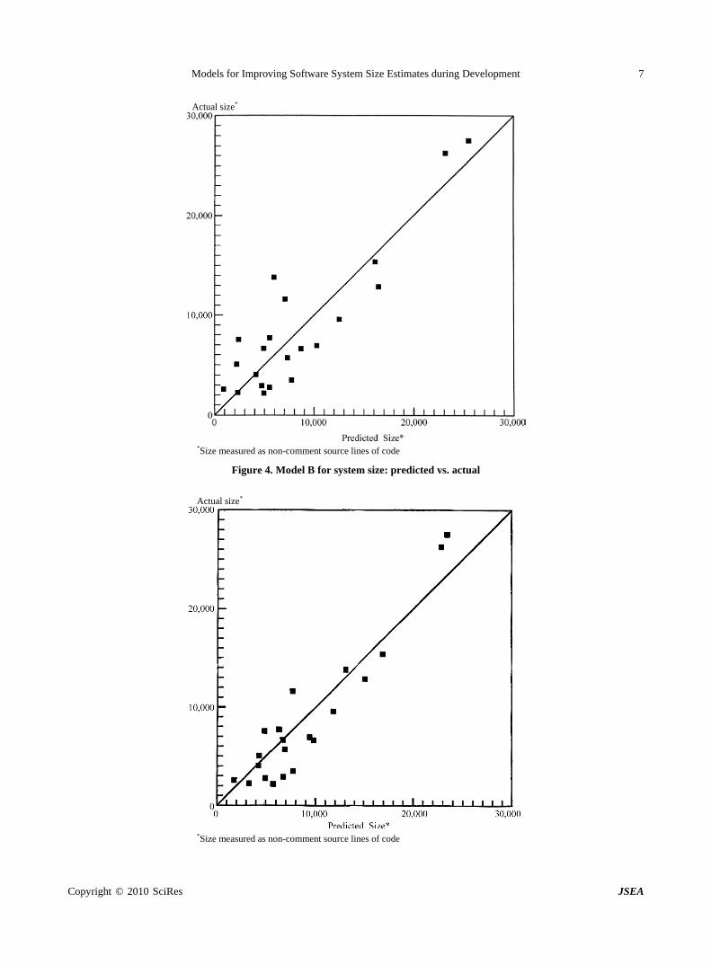
Figure 4. Model B for system size: predicted vs. actual
Actual size*
*Size measured as non-comment source lines of code
Copyright © 2010 SciRes JSEA
Models for Improving Software System Size Estimates during Development
Copyright © 2010 SciRes JSEA
8
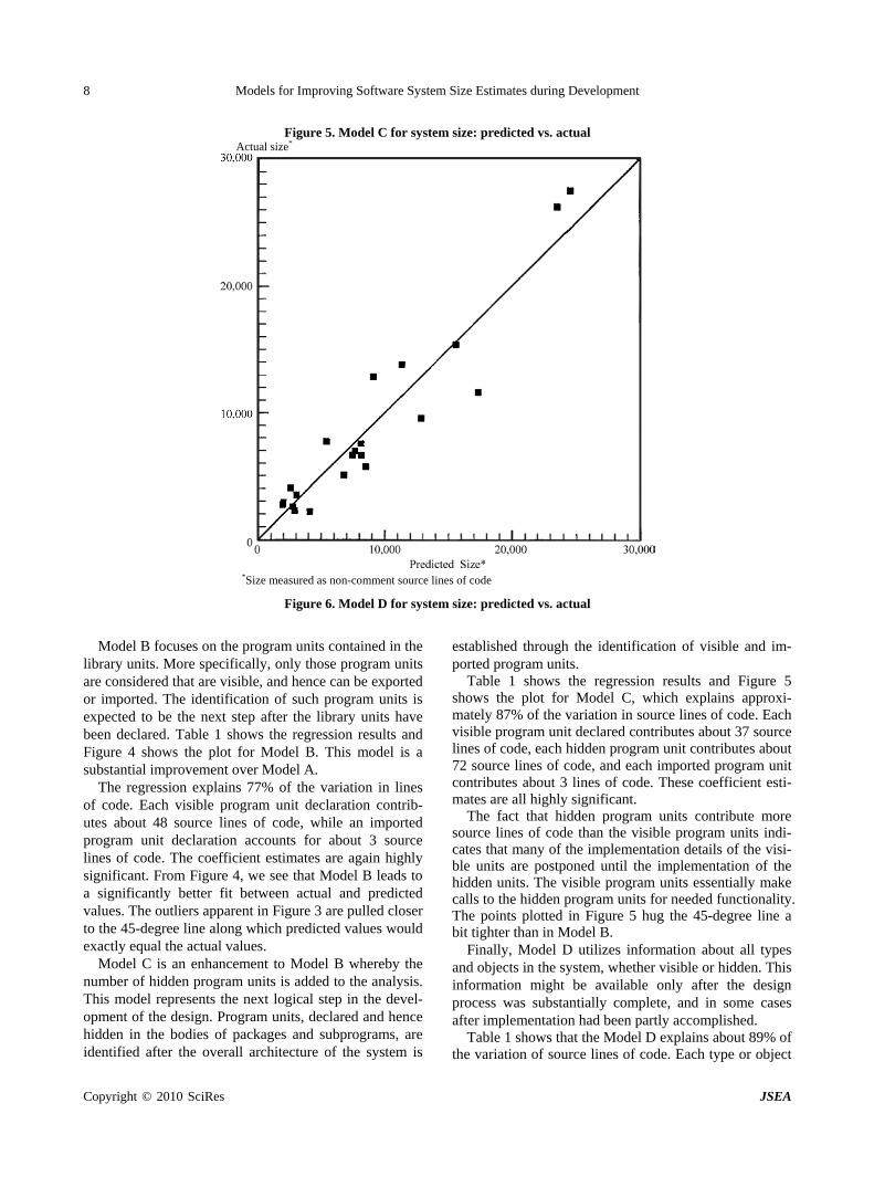
Figure 5. Model C for system size: predicted vs. actual Actual size*
*Size measured as non-comment source lines of code
Figure 6. Model D for system size: predicted vs. actual
Model B focuses on the program units contained in the
library units. More specifically, only those program units are considered that are visible, and hence can be exported or imported. The identification of such program units is expected to be the next step after the library units have been declared. Table 1 shows the regression results and Figure 4 shows the plot for Model B. This model is a substantial improvement over Model A.
The regression explains 77% of the variation in lines of code. Each visible program unit declaration contrib-utes about 48 source lines of code, while an imported program unit declaration accounts for about 3 source lines of code. The coefficient estimates are again highly significant. From Figure 4, we see that Model B leads to a significantly better fit between actual and predicted values. The outliers apparent in Figure 3 are pulled closer to the 45-degree line along which predicted values would exactly equal the actual values.
Model C is an enhancement to Model B whereby the number of hidden program units is added to the analysis. This model represents the next logical step in the devel-opment of the design. Program units, declared and hence hidden in the bodies of packages and subprograms, are identified after the overall architecture of the system is
established through the identification of visible and im-ported program units.
Table 1 shows the regression results and Figure 5 shows the plot for Model C, which explains approxi-mately 87% of the variation in source lines of code. Each visible program unit declared contributes about 37 source lines of code, each hidden program unit contributes about 72 source lines of code, and each imported program unit contributes about 3 lines of code. These coefficient esti-mates are all highly significant.
The fact that hidden program units contribute more source lines of code than the visible program units indi-cates that many of the implementation details of the visi-ble units are postponed until the implementation of the hidden units. The visible program units essentially make calls to the hidden program units for needed functionality. The points plotted in Figure 5 hug the 45-degree line a bit tighter than in Model B.
Finally, Model D utilizes information about all types and objects in the system, whether visible or hidden. This information might be available only after the design process was substantially complete, and in some cases after implementation had been partly accomplished.
Table 1 shows that the Model D explains about 89% of the variation of source lines of code. Each type or object
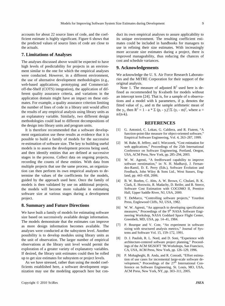
Models for Improving Software System Size Estimates during Development 9
accounts for about 22 source lines of code, and the coef-ficient estimate is highly significant. Figure 6 shows that the predicted values of source lines of code are close to the actuals.
7. Limitations of Analyses
The analyses discussed above would be expected to have high levels of predictability for projects in an environ-ment similar to the one for which the empirical analyses were conducted. However, in a different environment, the use of alternative development methodologies (e.g., web-based applications, prototyping and Commercial- off-the-Shelf (COTS) integration), the application of dif-ferent quality assurance criteria, and variations in the application domain might have an impact on these esti-mates. For example, a quality assurance criterion limiting the number of lines of code in a library unit would affect the results of any empirical analysis using library units as an explanatory variable. Similarly, two different design methodologies could lead to different decompositions of the design into library units and program units.
It is therefore recommended that a software develop-ment organization use these results as evidence that it is possible to build a family of models for the successive re-estimation of software size. The key to building useful models is to assess the development process being used, and then identify entities that are defined at successive stages in the process. Collect data on ongoing projects, recording the counts of these entities. With data from multiple projects that use the same process, an organiza-tion can then perform its own empirical analyses to de-termine the values of the coefficients for the models, guided by the approach used here. Once the family of models is then validated by use on additional projects, the models will become more valuable in estimating software size at various stages during a development project.
8. Summary and Future Directions
We have built a family of models for estimating software size based on successively available design information. The models demonstrate that the estimates can improve as more design information becomes available. The analyses were conducted at the subsystem level. Another possibility is to develop modules using library units as the unit of observation. The larger number of empirical observations at the library unit level would permit the exploration of a greater variety of explanatory variables. If desired, the library unit estimates could then be rolled up to get size estimates for subsystem or project levels.
As we have stressed, rather than using the model coef-ficients established here, a software development orga- nization may use the modeling approach here but con-
duct its own empirical analyses to assure applicability to its unique environment. The resulting coefficient esti-mates could be included in handbooks for managers to use in refining their size estimates. With increasingly more accurate size estimates during a project, there is improved manageability, thus reducing the chances of cost and schedule variances.
9. Acknowledgements
We acknowledge the U. S. Air Force Research Laborato-ries and the MITRE Corporation for their support of the original analysis.
Note 1. The measure of adjusted R2 used here is de-fined as recommended by Kvalseth for models without an intercept term [24]. That is, for a sample of n observa-tions and a model with k parameters, if pi denotes the fitted value of yi, and m the sample arithmetic mean of the yi, then R2 = 1 - a * (pi - yi)
2/ (yi - m)2, where a = n/(n-k).
REFERENCES [1] G. Antoniol, C. Lokan, G. Caldiera, and R. Fiutem, “A
function-point-like measure for object-oriented software,” Empirical Software Engineering, Vol. 4, 263–287, 1999.
[2] M. Ruhe, R. Jeffrey, and I. Wieczorek, “Cost estimation for web applications,” Proceedings of the 25th International Conference on Software Engineering, Portland, Oregon, USA, ACM Press, New York, pp. 285–294, 2003.
[3] W. W. Agresti, “A feedforward capability to improve software reestimation,” in: N. H. Madhavji, J. Fernan-dez-Ramil, D. E. Perry (Eds.), Software Evolution and Feedback, John Wiley & Sons Ltd., West Sussex, Eng-land, pp. 443–458, 2006.
[4] B. W. Boehm, C. Abts, A. W. Brown, C. Chulani, B. K. Clark, E. Horowitz, R. Madachy, D. Reifer, and B. Steece, Software Cost Estimation with COCOMO II, Prentice Hall, Upper Saddle River, NJ, USA, 2000.
[5] T. DeMarco, “Controlling software projects,” Yourdon Press, Englewood Cliffs, NJ, USA, 1982.
[6] W. W. Agresti, “An approach to developing specification measures,” Proceedings of the 9th NASA Software Engi-neering Workshop, NASA Goddard Space Flight Center, Greenbelt, MD, USA, pp. 14–41, 1984.
[7] P. Bourque and V. Cote, “An experiment in software sizing with structured analysis metrics,” Journal of Sys-tems and Software Vol. 15, 159–172, 1991.
[8] D. J. Paulish, R. L. Nord, and D. Soni, “Experience with architecture-centered software project planning,” Proceed-ings of the ACM SIGSOFT ’96 Workshops, San Francisco, CA, USA, ACM Press, New York, pp. 126–129, 1996.
[9] P. Mohagheghi, B. Anda, and R. Conradi, “Effort estima-tion of use cases for incremental large-scale software de-velopment,” Proceedings of the 27th International Con-ference on Software Engineering, St. Louis, MO, USA, ACM Press, New York, NY, pp. 303–311, 2005.
Copyright © 2010 SciRes JSEA
Models for Improving Software System Size Estimates during Development
Copyright © 2010 SciRes JSEA
10
[10] S. L. Pfleeger, “Model of software effort and productiv-ity,” Information and Software Technology, Vol. 33, 224–231, 1991.
[11] R. L. Jensen and J. W. Bartley, “Parametric estimation of programming effort: An object–oriented approach,” Jour-nal of Systems and Software, Vol. 15, pp. 107–114. 1991.
[12] L. Laranjeira, “Software size estimation of object–oriented systems,” IEEE Transactions on Software Engineering, Vol. 16, 510–522, 1990.
[13] A. Minkiewicz, “The evolution of software size: A search for value,” CROSSTALK, Vol. 22, No. 3, pp. 23–26, 2009.
[14] P. Fraternali, M. Tisi, and A. Bongio, “Automating func-tion point analysis with model driven development,” Pro-ceedings of the Conference of the Center for Advanced Studies on Collaborative Research, Toronto, Canada, ACM Press, New York, pp. 1–12, 2006.
[15] A. Albrecht and J. Gaffney, “Software function, source lines of code and development effort prediction,” IEEE Transactions on Software Engineering, Vol. 9, 639–648, 1983.
[16] H. B. K. Tan, Y. Zhao, and H. Zhang, “Estimating LOC for information systems from their conceptual data mod-els,” Proceedings of the 28th International Conference on Software Engineering, Shanghai, China, ACM Press, New York, pp. 321–330, 2006.
[17] S. Diev, “Software estimation in the maintenance con-text,” ACM Software Engineering Notes, Vol. 31, No. 2
pp. 1–8, 2006.
[18] W. Fornaciari, F. Salice, U. Bondi, and E. Magini, “De-velopment cost and size estimation from high-level speci-fications,” Proceedings of the Ninth International Sympo-sium on Hardware/Software Codesign, Copenhagen, Denmark, ACM Press, New York, NY, pp. 86–91, 2001.
[19] A. Zivkovic, I. Rozman, and M. Hericko, “Automated software size estimation based on function points using UML models,” Information and Software Technology, Vol. 47, pp. 881–890, 2005
[20] M. Hericko and A. Zivkovic, “The size and effort esti-mates in iterative development,” Information and Soft-ware Technology, Vol. 50, pp. 772–781, 2008.
[21] W. Royce, “TRW's Ada process model for incremental development of large software systems,” Proceedings of the 12th International Conference on Software Engineer-ing, Nice, France, pp. 2–11, 1990,
[22] F. E. McGarry and W. W. Agresti, “Measuring Ada for software development in the Software Engineering Labo-ratory,” Journal of Systems and Software, Vol. 9, pp. 149–159, 1989.
[23] D. Doubleday, “ASAP: An Ada static source code ana-lyzer program,” Technical Report 1895, Department of Computer Science, University of Maryland, College Park, MD USA, 1987.
[24] T. O. Kvalseth, “Cautionary note about R2,” The Ameri-can Statistician, Vol. 39, pp. 279–285, 1985.
J. Software Engineering & Applications, 2010, 3: 11-26 doi:10.4236/jsea.2010.31002 Published Online January 2010 (http://www.SciRP.org/journal/jsea)
Copyright © 2010 SciRes JSEA
11
A Massively Parallel Re-Configurable Mesh Computer Emulator: Design, Modeling and Realization
Mohamed YOUSSFI2, Omar BOUATTANE1, Mohamed O. BENSALAH2
1E. N. S. E. T, Bd Hassan II, BP, Mohammedia Morocco; 2Faculté Des Sciences Université Mohamed V Agdal Rabat Morocco. Email: [email protected], [email protected] Received November 4th, 2009; revised November 26th, 2009; accepted December 19th, 2009.
ABSTRACT
Emulating massively parallel computer architectures represents a very important tool for the parallel programmers. It allows them to implement and validate their algorithms. Due to the high cost of the massively parallel real machines, they remain unavailable and not popular in the parallel computing community. The goal of this paper is to present an elaborated emulator of a 2-D massively parallel re-configurable mesh computer of size n x n processing elements (PE). Basing on the object modeling method, we develop a hard kernel of a parallel virtual machine in which we translate all the physical properties of its different components. A parallel programming language and its compiler are also devel-oped to edit, compile and run programs. The developed emulator is a multi platform system. It can be installed in any sequential computer whatever may be its operating system and its processing unit technology (CPU). The size n x n of this virtual re-configurable mesh is not limited; it depends just on the performance of the sequential machine supporting the emulator. Keywords: Parallel processing, Object Modeling, Re-Configurable Mesh Computer, Emulation, XML, Parallel Virtual
Machine
1. Introduction
Recently, in the data analysis and signal processing do-main, the analysis tools, the computation methods and their technological computational models, have known a very high level of progress. This progress has oriented the scientists toward new computation strategies based on parallel approaches. Due to the large volume of data to be processed and to the large amount of computations needed to solve a given problem, the basic idea is to split tasks and data so that we can easily perform their corre-sponding algorithms concurrently on different physical computational units. Naturally, the use of the parallel approaches implies important data exchange between computational units. Subsequently, this generates new problems of data exchange and communications. To manage these communications, it is important to examine how the data in query are organized. This examination leads to several parallel algorithms and several corre-sponding computational architectures. Actually, we dis-tinguish several computer architectures, starting from a single processor computer model, until the massively fine grained parallel machines having a large amount of processing elements interconnected according to several topological networks. Indeed, the analysis of the per-
formance enhancement in terms of processing ability and execution speed must take into account the data compu-tation difficulties and addressing management problem of these data. With relation to the last problem, it seems that the classical VON NEUMANN processor model is not able to respond to all the mentioned constraints. Fur-thermore, the optimized software realized for some cases have quickly demonstrated the limits of this model.
The need of the new architectures and the processor efficiency improvement has been excited and encouraged by the VLSI development. As a result, we have seen the new processor technologies (e.g. Reduced Instruction Set Computer “RISC”, Transputer, Digital Signal Processor “DSP”, Cellular automata etc.) and the parallel intercon-nection of fine grained networks (e.g. Linear, 2-D grid of processors, pyramidal architectures, cubic and hyper cu-bic connexion machines, etc.)
In this paper, our study is focused on a fine grained parallel architecture that has been largely studied in the literature and for which several parallel algorithms for scientific calculus were developed. From the theoretical point of view, each computational model has its motiva-tions and its exciting proofs. In the practice, some models were technologically realized and served as real compu-tational supports, but some others remain in their theo-
A Massively Parallel Re-Configurable Mesh Computer Emulator: Design, Modeling and Realization 12
retical proposition state. They are not realized because of their technological complexities and to their very high production cost. The computational model that is con-cerned in our work has known a very large technological progress. At first, it was viewed as a simple grid of cel-lular automata, after some technological enhancement, the cellular automaton became a fine grained processing element and the resulted grid became the mesh connected computer MCC [1]. Using some additional communica-tion Buses, the MCC became the mesh with multiple broadcast [2] and polymorphic torus [3]. Finally, we speak about the reconfigurable mesh computer (RMC) that integrates a reconfiguration network at each proc-essing element [4,5].
From the algorithmic point of view, several authors were developed new parallel algorithms for data proc-essing and scientific calculus. These algorithms were assigned to be implemented in the architectures men-tioned above. Also, they are established using parallel approaches in order to reduce their complexities in term of execution times.
In order to facilitate for each parallel programmer the task of validation and program tests (even if he has not a real parallel machine that supports his algorithms), the emulating solutions were proposed in the literature to elaborate some virtual systems to perform the algorithms. The emulated systems may be specific as in [21,22] or of general behaviors as in [19,20].
In this context, we present in this paper a virtual tool to emulate an RMC, in which we can easily implement parallel SIMD algorithms. It is a virtual RMC platform of size (n x m) processing elements (PE), where n is the number of rows in the matrix an m is the number of columns. Without loss of generality, we consider n = m and we speak about a squared matrix of n² PE’s.
This emulator allows the scientists to overflow the problem of real RMC availability. (i.e. at this time the RMC machine is not yet popular due to its high cost).
Using this emulator, we propose an extended virtual RMC model, which translates all the functionalities of a real machine. This model can be easily extended to per-form other advanced functionalities required by the mul-tiplicity of the algorithmic techniques. In order to reach this virtual machine result, we started by the object mod-eling of all the components of the RMC such as the n x n grid, its processing element PE, its connexion buses and so. To describe in more details the different steps of this emulator realization, we organize this paper as follows: Section II presents the real RMC model and the essential properties of its components. The object modeling of the RMC and some related details are given in section III. The next section, presents some parallel programs and their implementation on our virtual machine to illustrate the use of some established parallel instructions. Notice that, to avoid the upload of this paper, the complete set of
instructions established for our platform is not presented in more details. We present just some examples of testing programs that involve some scientific computations such as basic matrix computation, data processing and image processing. Finally, the last section gives some conclud-ing remarks and some exploiting perspectives of our vir-tual machine.
2. Parallel Computational Model
2.1 Presentation
The parallel architectures have known a large develop-ment these recent years. They are presented in numerous topological shapes, such as, linear, planar, pyramidal, cubic and hyper cubic networks. This large number of architectures requires an adequate classification taking into account several criteria. Among these criteria, we distinguish for example, the size of the machine, its autonomy of addressing and connexion, data type used etc. This classification allows the programmer to choose an appropriate computational model to perform the pro-grams. Several proposed classifications were described in the literature; the diversity of the architectural solutions makes difficult the establishment of a general taxonomy. The well known classification is based on multiplicity of the instruction and data flows. It proposed four types of data machines, they are: the Single Instruction Single Data (S.I.S.D), single Instruction Multiple Data (S.I. M.D), multiple Instruction Single Data (M.I.S.D) and multiple Instruction Multiple Data (M.I.M.D) machines. Throughout this classification, the concerned model in this work is the Re-configurable Mesh Computer. It is the 2-D planar grid or matrix of n x n processing ele-ments (PE). It is an S.I.M.D structure where in the word model the PE’s use data buses of width at most log2 n bits. Also, in this model, the PE’s has the autonomy of operation, addressing and connexion.
2.2 Topology and Structure
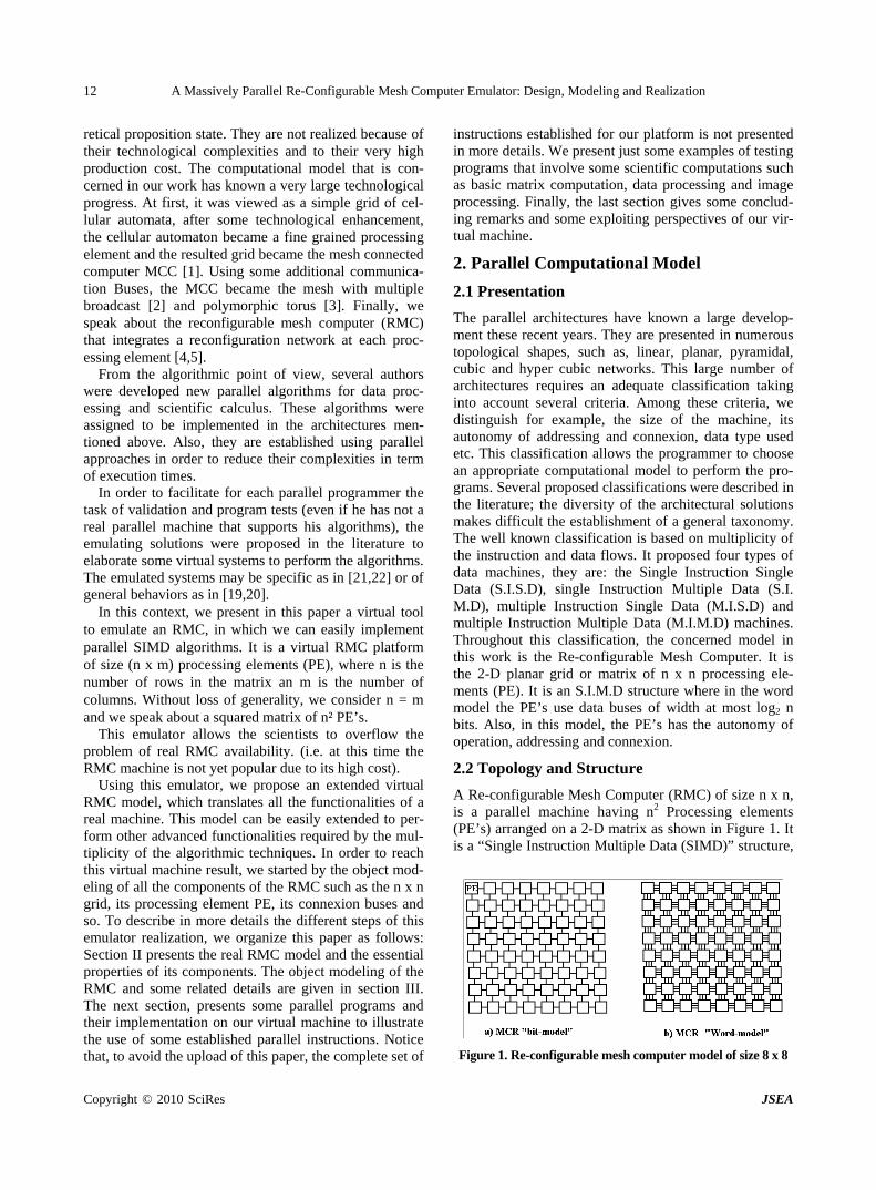
A Re-configurable Mesh Computer (RMC) of size n x n, is a parallel machine having n2 Processing elements (PE’s) arranged on a 2-D matrix as shown in Figure 1. It is a “Single Instruction Multiple Data (SIMD)” structure,
Figure 1. Re-configurable mesh computer model of size 8 x 8
Copyright © 2010 SciRes JSEA
A Massively Parallel Re-Configurable Mesh Computer Emulator: Design, Modeling and Realization 13
in which each PE(i, j) is localized in row i and column j. It has an identifier defined by ID = n x i + j. Each PE of the mesh is connected to its four neighbors (if they exist) by communication channels. It has a finite number of registers of size (log2 n) bits. The PE’s can carry out arithmetic and logical operations. They can also carry out reconfiguration operations to exchange data over the mesh.
The re-configurable networks that are presented as the processors matrix were improved considerably these last years. Indeed many theoretical and practical works ap-peared in the literature use this architecture as a compu-tational model [6–8]. More particularly the recent related works propose new re-configurable models [9–14]. These re-configurable networks are based on a dynamic change of the mesh shape. They are qualified as the polymorphic grids of processors.
These architectures are provided with an instruction set of reconfiguration in order to get several topological shapes according to the problem to be solved. They are presented typically in the form of a multidimensional network of processing elements connected to a commu-nication bus having a fixed number of wiring of In-put/output. When this bus is reduced to only one bit width, we speak about “bit-model” machine, whereas for a mesh of size n x n having a bus of width (log2 n bits), we speak about “Word-model” machine as in [9,15]. Figure 1, shows a 2-D representation of this model. Re-configuration is locally made by adjusting the bus switches at each PE. The control of these switches offers to the PE’s connection autonomy. Indeed, different PE’s can simultaneously select various switches to achieve a given configuration. This is based on local decisions made by each PE. Also, it is possible for all the PE’s of a selected group to carry out unconditional operations of configuration, where the PE’s carry out reconfiguration instructions to activate their switches.
2.3 Basic Operations of a PE
2.3.1 Arithmetic Operations Like any standard processor, the PE’s of the RMC
have an instruction set relating to the arithmetic and logical
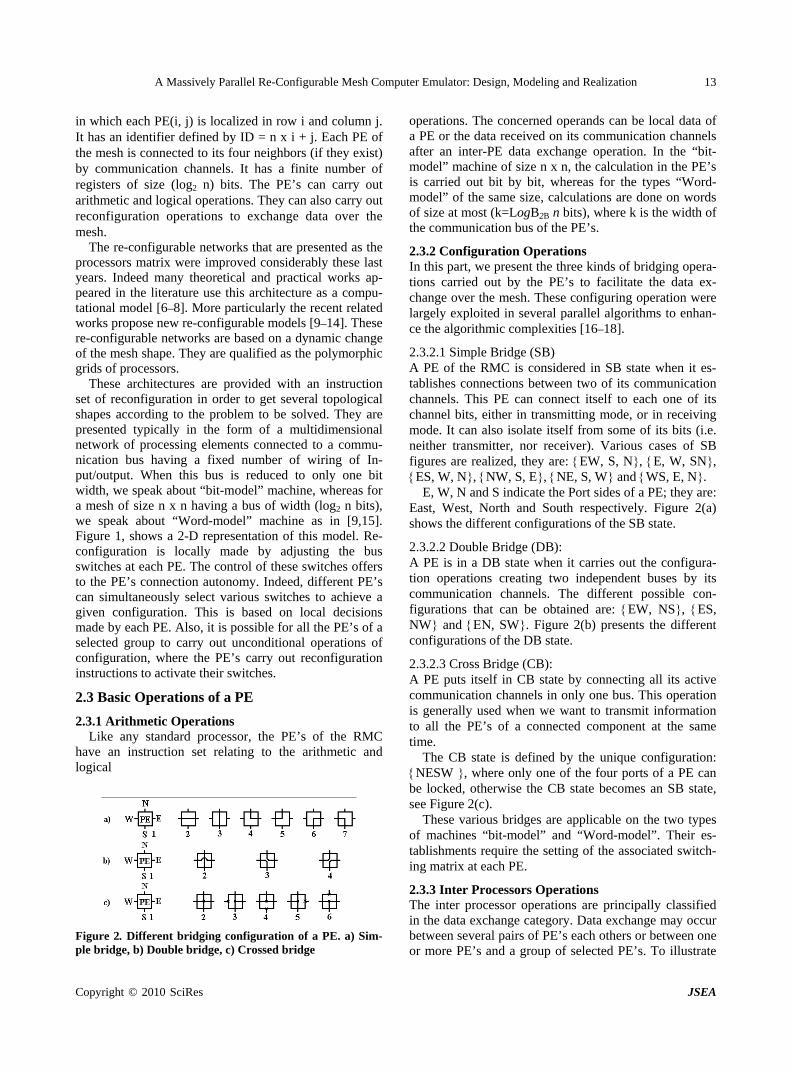
Figure 2. Different bridging configuration of a PE. a) Sim-ple bridge, b) Double bridge, c) Crossed bridge
operations. The concerned operands can be local data of a PE or the data received on its communication channels after an inter-PE data exchange operation. In the “bit-model” machine of size n x n, the calculation in the PE’s is carried out bit by bit, whereas for the types “Word- model” of the same size, calculations are done on words of size at most (k=LogB2B n bits), where k is the width of the communication bus of the PE’s.
2.3.2 Configuration Operations In this part, we present the three kinds of bridging opera-tions carried out by the PE’s to facilitate the data ex-change over the mesh. These configuring operation were largely exploited in several parallel algorithms to enhan- ce the algorithmic complexities [16–18].
2.3.2.1 Simple Bridge (SB) A PE of the RMC is considered in SB state when it es-tablishes connections between two of its communication channels. This PE can connect itself to each one of its channel bits, either in transmitting mode, or in receiving mode. It can also isolate itself from some of its bits (i.e. neither transmitter, nor receiver). Various cases of SB figures are realized, they are: EW, S, N, E, W, SN, ES, W, N, NW, S, E, NE, S, Wand WS, E, N.
E, W, N and S indicate the Port sides of a PE; they are: East, West, North and South respectively. Figure 2(a) shows the different configurations of the SB state.
2.3.2.2 Double Bridge (DB): A PE is in a DB state when it carries out the configura-tion operations creating two independent buses by its communication channels. The different possible con-figurations that can be obtained are: EW, NS, ES, NW and , SW. Figure 2(b) presents the different configurations of the DB state.
2.3.2.3 Cross Bridge (CB): A PE puts itself in CB state by connecting all its active communication channels in only one bus. This operation is generally used when we want to transmit information to all the PE’s of a connected component at the same time.
The CB state is defined by the unique configuration: NESW , where only one of the four ports of a PE can be locked, otherwise the CB state becomes an SB state, see Figure 2(c).
These various bridges are applicable on the two types of machines “bit-model” and “Word-model”. Their es-tablishments require the setting of the associated switch-ing matrix at each PE.
2.3.3 Inter Processors Operations The inter processor operations are principally classified in the data exchange category. Data exchange may occur between several pairs of PE’s each others or between one or more PE’s and a group of selected PE’s. To illustrate
Copyright © 2010 SciRes JSEA
A Massively Parallel Re-Configurable Mesh Computer Emulator: Design, Modeling and Realization 14
the concept of inter processor operations, we present an example of data exchange procedure named “Direct broadcasting”
The “Direct broadcasting” procedure consists of trans-mitting information from a given PE over a mesh re-sulted by the CB operation, to all the connected PE’s on this mesh. The complexity of this operation is: iteration. The necessary instructions are:
- All the PE’s go to the CB state. - All the PE’s couple themselves in receiving
mode on the resulted bridge, except for the PE which will transmit data. It must be coupled in transmitting mode.
- The transmitting PE transmits Data on its bridge. Thus all the receiver PE’s can read concurrently the same information on their ‘communication buses.
More details about the reconfiguration operations in technological point of view and communication cost are discussed in [3], where the polymorphic torus is equipped by the same reconfiguration network as the re-configurable mesh.
3. Object Modeling of the RMC
3.1 Presentation
As mentioned in the precedent section, the RMC is a set of processing elements arranged in a squared matrix. Each PE is modeled by an object defined by a state and a behavior.
The state of the PE object is represented by the values of its memory registers and its internal linked compo-nents, such as, its arithmetic and logical unit (ALU) and its four ports (East, West, North, South).
The PE behavior represents the set of operations that it can carry out. The kind of these operations is: arithmetic, logic, bus configuration (e.g. bridge operations) data ex-change, marking and unmarking a PE, etc. In addition to these operations, it may be necessary to add other spe-cific operations to delegate to a given PE a task to repre-sent a given group of PE’s in the RMC. In this case as in [12,17], the delegated PE is labeled Representative PE (RPE).
Generally, all the basically operations required by a PE belong to its object behavior section. Taking into account the object modeling of all the PE features, it seems that this approach is the appropriate tool to realize our paral-lel programming emulator.
Since the emulator environment is performed on a se-quential machine, a parallel to sequential mapping is needed. This means that the realized emulator requires three layouts:
- The sequential layout: It is the kernel of our project. It performs all the operations of the emulating program.
- The parallel layout: It represent the parallel pro-gramming RMC environment, where any parallel pro-
grammer can write, compile, debug and run its parallel program.
- The third layout is the intermediate one between parallel and sequential layouts. It realizes the mapping task, where each parallel instruction is converted into a set of sequential instructions.
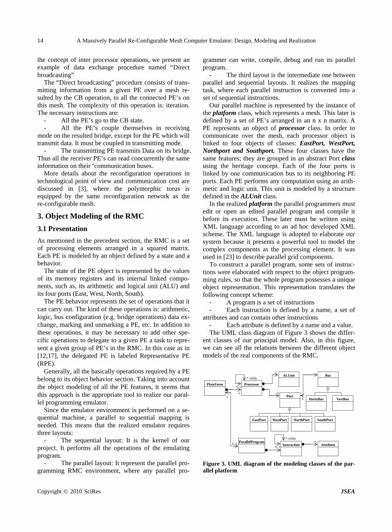
Our parallel machine is represented by the instance of the platform class, which represents a mesh. This later is defined by a set of PE’s arranged in an n x n matrix. A PE represents an object of processor class. In order to communicate over the mesh, each processor object is linked to four objects of classes: EastPort, WestPort, Northport and Southport. These four classes have the same features; they are grouped in an abstract Port class using the heritage concept. Each of the four ports is linked by one communication bus to its neighboring PE ports. Each PE performs any computation using an arith-metic and logic unit. This unit is modeled by a structure defined in the ALUnit class.
In the realized platform the parallel programmers must edit or open an edited parallel program and compile it before its execution. These later must be written using XML language according to an ad hoc developed XML scheme. The XML language is adopted to elaborate our system because it presents a powerful tool to model the complex components as the processing element. It was used in [23] to describe parallel grid components.
To construct a parallel program, some sets of instruc-tions were elaborated with respect to the object program- ming rules, so that the whole program possesses a unique object representation. This representation translates the following concept scheme:
- A program is a set of instructions - Each instruction is defined by a name, a set of
attributes and can contain other instructions - Each attribute is defined by a name and a value. The UML class diagram of Figure 3 shows the differ-
ent classes of our principal model. Also, in this figure, we can see all the relations between the different object models of the real components of the RMC.
PlateForm Processor
ALUnit
Port
EastPort WestPort NorthPort SouthPort
Bus
HorizBus VertBus
ParallelProgramInstruction Attribute
0..1
* childs
4
* 1
0..10..1
* childs *
*
1
Figure 3. UML diagram of the modeling classes of the par-allel platform
Copyright © 2010 SciRes JSEA
A Massively Parallel Re-Configurable Mesh Computer Emulator: Design, Modeling and Realization 15
Data Registers
idReg
Flag register
0 1 2 3 ......15
bridge
ALU
PORT
PORT
PORT
PORT
BUSBUS
BUS
iReg
jReg Reg[2]
Reg[1]
Reg[0]
Reg[n]
BUS
Figure 4. Representation of the components of a processing element model
3.2 Description of the RMC Model Classes
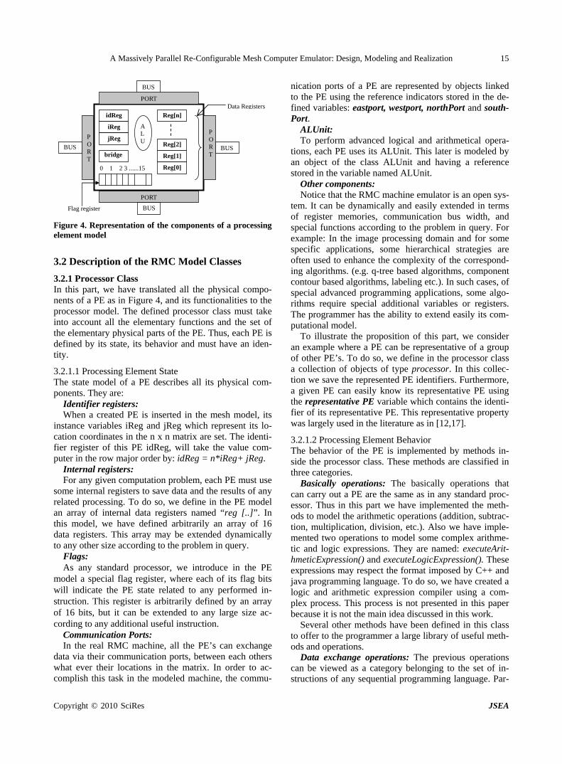
3.2.1 Processor Class In this part, we have translated all the physical compo-nents of a PE as in Figure 4, and its functionalities to the processor model. The defined processor class must take into account all the elementary functions and the set of the elementary physical parts of the PE. Thus, each PE is defined by its state, its behavior and must have an iden-tity.
3.2.1.1 Processing Element State The state model of a PE describes all its physical com-ponents. They are:
Identifier registers: When a created PE is inserted in the mesh model, its
instance variables iReg and jReg which represent its lo-cation coordinates in the n x n matrix are set. The identi-fier register of this PE idReg, will take the value com-puter in the row major order by: idReg = n*iReg+ jReg.
Internal registers: For any given computation problem, each PE must use
some internal registers to save data and the results of any related processing. To do so, we define in the PE model an array of internal data registers named “reg [..]”. In this model, we have defined arbitrarily an array of 16 data registers. This array may be extended dynamically to any other size according to the problem in query.
Flags: As any standard processor, we introduce in the PE
model a special flag register, where each of its flag bits will indicate the PE state related to any performed in-struction. This register is arbitrarily defined by an array of 16 bits, but it can be extended to any large size ac-cording to any additional useful instruction.
Communication Ports: In the real RMC machine, all the PE’s can exchange
data via their communication ports, between each others what ever their locations in the matrix. In order to ac-complish this task in the modeled machine, the commu-
nication ports of a PE are represented by objects linked to the PE using the reference indicators stored in the de-fined variables: eastport, westport, northPort and south- Port.
ALUnit: To perform advanced logical and arithmetical opera-
tions, each PE uses its ALUnit. This later is modeled by an object of the class ALUnit and having a reference stored in the variable named ALUnit.
Other components: Notice that the RMC machine emulator is an open sys-
tem. It can be dynamically and easily extended in terms of register memories, communication bus width, and special functions according to the problem in query. For example: In the image processing domain and for some specific applications, some hierarchical strategies are often used to enhance the complexity of the correspond-ing algorithms. (e.g. q-tree based algorithms, component contour based algorithms, labeling etc.). In such cases, of special advanced programming applications, some algo-rithms require special additional variables or registers. The programmer has the ability to extend easily its com-putational model.
To illustrate the proposition of this part, we consider an example where a PE can be representative of a group of other PE’s. To do so, we define in the processor class a collection of objects of type processor. In this collec-tion we save the represented PE identifiers. Furthermore, a given PE can easily know its representative PE using the representative PE variable which contains the identi-fier of its representative PE. This representative property was largely used in the literature as in [12,17].
3.2.1.2 Processing Element Behavior The behavior of the PE is implemented by methods in-side the processor class. These methods are classified in three categories.
Basically operations: The basically operations that can carry out a PE are the same as in any standard proc-essor. Thus in this part we have implemented the meth-ods to model the arithmetic operations (addition, subtrac-tion, multiplication, division, etc.). Also we have imple-mented two operations to model some complex arithme-tic and logic expressions. They are named: executeArit- hmeticExpression() and executeLogicExpression(). These expressions may respect the format imposed by C++ and java programming language. To do so, we have created a logic and arithmetic expression compiler using a com-plex process. This process is not presented in this paper because it is not the main idea discussed in this work.
Several other methods have been defined in this class to offer to the programmer a large library of useful meth- ods and operations.
Data exchange operations: The previous operations can be viewed as a category belonging to the set of in-structions of any sequential programming language. Par-
Copyright © 2010 SciRes JSEA
A Massively Parallel Re-Configurable Mesh Computer Emulator: Design, Modeling and Realization
Copyright © 2010 SciRes JSEA
16
allel programming is characterized by other types of in-structions. In fact, as mentioned above, the Peps of the RMC must collaborate between each others by exchang-ing data via their communication buses. Among the im-plemented methods of this category, we distinguish: sendValue (double v): This method allows the
PE to send a data value v to its neighboring PE’s accord-ing to its bridge configuration state. receiveData (double data, char port, byte regR):
Allows the PE to receive a data value on its port speci-fied by the parameter port and to store the received data in its register regR. sendAndReceiveData (char portS, byte regS,
char portR, byte regR): allows the PE to send the data value of its register regS on the port specified by the pa-rameter portS, and receive data on the port specified by the parameter portR, the PE stores the received data in its register regR. receiveAndSendWithOperation (ProcessPort po-
rt, String op): This method is used to receive data, exe-cute some operations on this data and send the result to other PE’s according to their bridge states.
Configuration operations: In the parallel program-ming domain and particularly in the SIMD computational models, the processing element can play several roles depending on its configurations. In the processor class, we have defined a set of methods to change and to know the actual configuration of the PE. During the execution phase of a given parallel program, it is necessary to point at each stage of this phase, the group of active PE’s. For these reasons, we define the methods select() and un-select() to select or unselect the Peps that are susceptible to execute or not the instructions. Among the selected PE’s, it is possible to assign for some specific instruc-tions the concerned PE’s using other methods to mark or unmark them. Thus, we define other methods, mark() and unmark() to distribute a Boolean label to each se-lected PE. This label can be integrated in the program as a test variable.
To determine the configuration state of a PE at any given stage, some other appropriate operations are intro-duced.
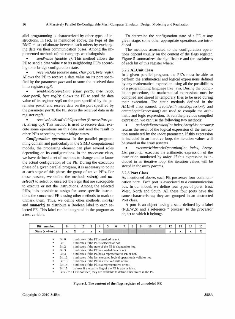
The methods associated to the configuration opera-tions depend usually on the content of the flags register. Figure 5 summarizes the significance and the usefulness of each bit of this register where:
3.2.2 ALUnit Class In a given parallel program, the PE’s must be able to perform the arithmetical and logical expressions defined by any mathematical expression using all the possibilities of a programming language like java. During the compi-lation procedure, the mathematical expressions must be compiled and stored in temporary files to be used during their execution. The static methods defined in the ALUnit class named, createArithmeticExpression() and createLogicExpression() are used to compile the arith-metic and logic expression. To run the previous compiled expression, we can use the following two methods: getLogicExpression(int index,ArrayList params):
returns the result of the logical expression of the instruc-tion numbered by the index parameter. If this expression is included in an iterative loop, the iteration values will be stored in the array params. executeArithmericOperation(int index, Array-
List params): executes the arithmetic expression of the instruction numbered by index. If this expression is in-cluded in an iterative loop, the iteration values will be stored in the array params.
3.2.3 Port Class As mentioned above, each PE possesses four communi-cation ports. Each port is associated to a communication bus. In our model, we define four types of ports: East, West, North and South. All these four ports have the same characteristics; they are grouped in an abstracted Port class.
A port is an object having a state defined by a label (N,E,W,S) and a reference ” process” to the processor object to which it belongs.
Bit number 0 1 2 3 4 5 6 7 8 9 10 11 12 13 14 15
State (x =0 or 1) x X x x x x x x X
Bit 0 : indicates if the PE is marked or not. Bit 1 : indicates if the PE is selected or not. Bit 2 : indicates if the state of the PE is changed or not. Bit 3 : indicates if the PE has loaded data or not. Bit 4 : indicates if the PE has a representative PE or not. Bit 12 : indicates if the last executed logical operation is valid or not. Bit 13 : indicates if the PE has received data or not. Bit 14 : indicates if the PE is a representative or not. Bit 15 : shows if the parity flag of the PE is true or false. Bits 5 to 11 are not used, they are available to define other states in the PE.
Figure 5. The content of the flags register of a modeled PE
A Massively Parallel Re-Configurable Mesh Computer Emulator: Design, Modeling and Realization 17
PlateForm
ParalleleProgram
fileName: String
compile(): void run() : void
1
1
Instruction
name: String
execute(): void
1..*Attribute
name: String value : String
0..*1..1 1..1
0..*0..1
Figure 6. The UML class diagram of a program
A port can be locked by its PE using a Boolean in-
stance variable locked. Since each port is associated to a communication bus, the reference to this bus must be stored in this class. Finally, each port must have one con-figuration variable to specify how the data can be trans-ferred from the port to its communication bus.
Example: If we consider an 8 bits communication bus, the defaults configuration of a port is defined by the or-der «01234567». This means that the bit i (i=0 to 7) of the port is linked to the bit i of the bus. In this case the data sent over the port is transmitted without any trans-formation. While in the configuration «70123456» the bit 0 of the port is connected to bit 1 of the bus and the bit i (i=1 to 6) is linked to bit i+1 of the bus. The bit 7 of the port is linked to bit 0 of the bus. This means that the transmitted data is left rotated over the bus. This kind of commutation operations on ports are often used in several parallel programs [9].
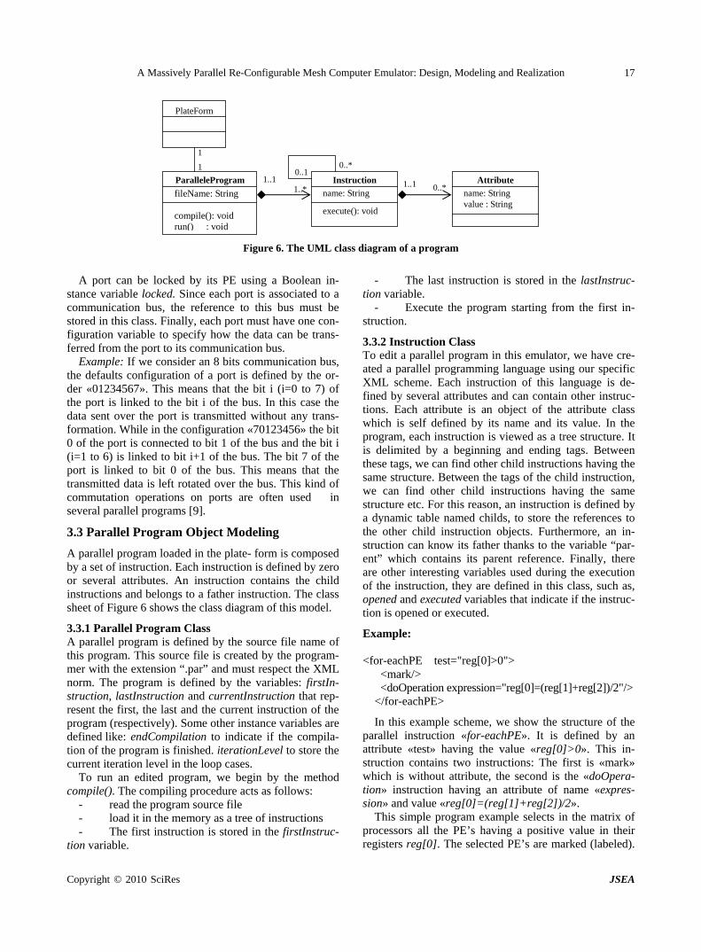
3.3 Parallel Program Object Modeling
A parallel program loaded in the plate- form is composed by a set of instruction. Each instruction is defined by zero or several attributes. An instruction contains the child instructions and belongs to a father instruction. The class sheet of Figure 6 shows the class diagram of this model.
3.3.1 Parallel Program Class A parallel program is defined by the source file name of this program. This source file is created by the program-mer with the extension “.par” and must respect the XML norm. The program is defined by the variables: firstIn-struction, lastInstruction and currentInstruction that rep-resent the first, the last and the current instruction of the program (respectively). Some other instance variables are defined like: endCompilation to indicate if the compila-tion of the program is finished. iterationLevel to store the current iteration level in the loop cases.
To run an edited program, we begin by the method compile(). The compiling procedure acts as follows:
- read the program source file - load it in the memory as a tree of instructions - The first instruction is stored in the firstInstruc-
tion variable.
- The last instruction is stored in the lastInstruc-tion variable.
- Execute the program starting from the first in-struction.
3.3.2 Instruction Class To edit a parallel program in this emulator, we have cre-ated a parallel programming language using our specific XML scheme. Each instruction of this language is de-fined by several attributes and can contain other instruc-tions. Each attribute is an object of the attribute class which is self defined by its name and its value. In the program, each instruction is viewed as a tree structure. It is delimited by a beginning and ending tags. Between these tags, we can find other child instructions having the same structure. Between the tags of the child instruction, we can find other child instructions having the same structure etc. For this reason, an instruction is defined by a dynamic table named childs, to store the references to the other child instruction objects. Furthermore, an in-struction can know its father thanks to the variable “par-ent” which contains its parent reference. Finally, there are other interesting variables used during the execution of the instruction, they are defined in this class, such as, opened and executed variables that indicate if the instruc-tion is opened or executed.
Example:
<for-eachPE test="reg[0]>0"> <mark/> <doOperation expression="reg[0]=(reg[1]+reg[2])/2"/>
</for-eachPE>
In this example scheme, we show the structure of the parallel instruction «for-eachPE». It is defined by an attribute «test» having the value «reg[0]>0». This in-struction contains two instructions: The first is «mark» which is without attribute, the second is the «doOpera-tion» instruction having an attribute of name «expres-sion» and value «reg[0]=(reg[1]+reg[2])/2».
This simple program example selects in the matrix of processors all the PE’s having a positive value in their registers reg[0]. The selected PE’s are marked (labeled).
Copyright © 2010 SciRes JSEA
A Massively Parallel Re-Configurable Mesh Computer Emulator: Design, Modeling and Realization 18
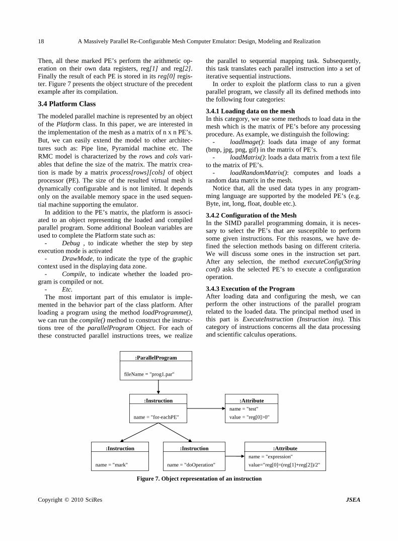
Then, all these marked PE’s perform the arithmetic op-eration on their own data registers, reg[1] and reg[2]. Finally the result of each PE is stored in its reg[0] regis-ter. Figure 7 presents the object structure of the precedent example after its compilation.
3.4 Platform Class
The modeled parallel machine is represented by an object of the Platform class. In this paper, we are interested in the implementation of the mesh as a matrix of n x n PE’s. But, we can easily extend the model to other architec-tures such as: Pipe line, Pyramidal machine etc. The RMC model is characterized by the rows and cols vari-ables that define the size of the matrix. The matrix crea-tion is made by a matrix process[rows][cols] of object processor (PE). The size of the resulted virtual mesh is dynamically configurable and is not limited. It depends only on the available memory space in the used sequen-tial machine supporting the emulator.
In addition to the PE’s matrix, the platform is associ-ated to an object representing the loaded and compiled parallel program. Some additional Boolean variables are used to complete the Platform state such as:
- Debug , to indicate whether the step by step execution mode is activated
- DrawMode, to indicate the type of the graphic context used in the displaying data zone.
- Compile, to indicate whether the loaded pro-gram is compiled or not.
- Etc. The most important part of this emulator is imple-
mented in the behavior part of the class platform. After loading a program using the method loadProgramme(), we can run the compile() method to construct the instruc-tions tree of the parallelProgram Object. For each of these constructed parallel instructions trees, we realize
the parallel to sequential mapping task. Subsequently, this task translates each parallel instruction into a set of iterative sequential instructions.
In order to exploit the platform class to run a given parallel program, we classify all its defined methods into the following four categories:
3.4.1 Loading data on the mesh In this category, we use some methods to load data in the mesh which is the matrix of PE’s before any processing procedure. As example, we distinguish the following:
- loadImage(): loads data image of any format (bmp, jpg, png, gif) in the matrix of PE’s.
- loadMatrix(): loads a data matrix from a text file to the matrix of PE’s.
- loadRandomMatrix(): computes and loads a random data matrix in the mesh.
Notice that, all the used data types in any program-ming language are supported by the modeled PE’s (e.g. Byte, int, long, float, double etc.).
3.4.2 Configuration of the Mesh In the SIMD parallel programming domain, it is neces-sary to select the PE’s that are susceptible to perform some given instructions. For this reasons, we have de-fined the selection methods basing on different criteria. We will discuss some ones in the instruction set part. After any selection, the method executeConfig(String conf) asks the selected PE’s to execute a configuration operation.
3.4.3 Execution of the Program After loading data and configuring the mesh, we can perform the other instructions of the parallel program related to the loaded data. The principal method used in this part is ExecuteInstruction (Instruction ins). This category of instructions concerns all the data processing and scientific calculus operations.
:ParallelProgram
fileName = "prog1.par"
:Instruction
name = "for-eachPE"
:Attribute
name = "test"
value = "reg[0]>0"
:Instruction
name = "mark"
:Instruction
name = "doOperation"
:Attribute
name = "expression"
value="reg[0]=(reg[1]+reg[2])/2"
Figure 7. Object representation of an instruction
Copyright © 2010 SciRes JSEA

A Massively Parallel Re-Configurable Mesh Computer Emulator: Design, Modeling and Realization 19
3.4.4 Displaying Results During the program execution, we can insert some methods to display the results using several numerical formats. For example, we can use the text format to ob-serve the contents of different registers of the PE’s or to display any data results in text format. A graphical con-text is also available in our platform to display other re-sults in graphical mode such as curves and images.
3.5 Instruction Sets
In order to construct our programming language, we have developed an XML scheme which defines the parallel instruction sets to edit parallel programs.
A program must begin by the tag <prog> and ends by </prog> tag. Between the two tags we can edit the in-structions.
Each instruction begins by the tag indicating the in-struction name and ends by the tag indicating the end of the instruction. An instruction can be defined by several attributes, it can encapsulate other instructions.
As for the real RMC, the emulating platform has three categories of instruction sets. They are presented as fol-lows:
3.5.1 Instructions for PE Configuration In the SIMD architectures, the parallel programming is based on a fundamental principle, where it is necessary to select, mark and bridge the PE’s concerned by the in-struction execution. The configuration instruction set is expressed by the following actions:
Selecting: This action is expressed by the instruction:
<for-eachPE cols= "valCols" rows= "valRows" test= "expression_logic" direction="">
… ( Operations to be executed ) </for-eachPE>
The attributes “cols” and “rows” define the concerned columns and rows. When several columns and rows are concerned, they are separated by commas.
The attribute direction is defined by a string to indi-cate the direction of the selected group of PE’s starting from the PE of coordinates indicated in “rows” and “cols” attributes. The possible direction attributes are: «RE» or «RW»: to define the direction East or
West along a Row. «CN»or «CS»: to define the direction North or
South along a Column. «DNE» or «DNW»: for the direction North-Est
or North-West along a diagonal. «DSE» or «DSW»: for the direction South-Est
or South-West along a diagonal. The attribute test is used to select a set of PE’s satis-
fying the condition defined by a logical expression. For example, in the expression (test="reg[1]>10") ,
the selected PE’s are those having in their reg[1] the
values greater than 10. Marking: This action uses the following instructions:
<mark type="true| false" />: to mark a PE if its at-tribute type is true and unmark it, if this attribute is false.
<mark />: to mark a PE without condition. <unMark />: to Unmark a PE without condition.
Bridging: As mentioned in the physical description of the RMC, a PE can be configured in three kinds of bridges: simple, double or crossed bridge. These bridging states are implemented by the following instruction:
<bridge type= "SB-WE|SB-NS | SB-WN | SB-WS | SB-NE | SB-SE | DB-WN-SE | DB-NE-SW |DB-NS-WE | CB-WNE | CB-NES | CB-ESW | CB-SWN | CB-WNES | NB"/>.
This instruction named bridge is used by a PE by de-fining its kind in the attribute type.
The attribute type is formulated by: - Defining the kind by: SB = Simple Bridge, DB=
Double Bridge and CB= Crossed Bridge. - Defining the direction of the bridge E,W,N and
S for East, West, North and South (respectively) The SB configurations are: {SB-NS, SB-WE, SB-WN,
SB-WS, SB-NE, SB-SE, SB-WS}. At any mentioned configuration the data is bypassing
bi-directionally the PE over its bridges. The DB configurations are: {DB-WN-SE, DB-NE-
SW, DB-NS-WE}. In this case, two communication bridges are con-
structed by a PE. So, two data can simultaneously bypass bi-directionally the PE.
The CB configurations are: {CB-WNE, CB-NES, CB- ESW, CB-SWN, CB-WNES}.
In this case, the only one obtained communication channel links at least three ports of the PE.
Notice that, to return back to the no bridge state from any bridge configuration, we use the instruction bridge with an attribute type {NB} to specify No Bridge.
3.5.2 Arithmetic / Logic Instructions and Control Structures
In the modeled parallel programming language, the arithmetic and logic instructions are expressed using the format defined bellow. In addition to the reconfiguration operations, each PE of the RMC can carry out a set of arithmetic/logic instructions and control structures. These instructions are formatted as defined in the following examples:
- Arithmetic / logic instructions
<inc reg="numReg"/>: means: reg [numReg] = reg [numReg]+1;
<dec reg="numReg"/>: means: reg [num-Reg] = reg [numReg]-1;
Copyright © 2010 SciRes JSEA

A Massively Parallel Re-Configurable Mesh Computer Emulator: Design, Modeling and Realization 20
<add reg="numReg" value= "val"/>: means : reg [numReg] = reg [numReg]+Value;
<sub reg="numReg" value= "val"/>: means : reg [numReg] = reg [numReg]-Value;
<mult reg="numReg" value= "val"/>: means : reg [numReg] = reg [numReg]*Value;
<div reg="numReg" value= "val"/>: means : reg [numReg] = reg [numReg]/Value;
<doOperation expression= "arithmetic_expre-
ssion" />: This instruction executes the arithmetic ex-pression specified by the expression attribute. We have developped a compiler to execute all the possible arith-metical expressions according to the same syntaxes of the C and Java language.
- Control structures The control structures defined for our platform are the
same as the well known for any language. The following examples give the presentation of some structures.
<if test= "logic_ expression"> … instructions … </if>
<for from= "begin_val" to= "end_val">… instruc-tions ...</for>
<while test= "logic_expression">… instruction- s …</while>
3.5.3 Data Exchange Instructions The third instruction set developed for this emulator concerns the specific instructions to exchange data be-tween the PE’s of the RMC. This set allows the pro-grammer to manipulate some new concepts introduced in the parallel SIMD algorithms. These instructions use the four Port objects of each PE to send, receive and broad-cast data over the mesh. Among the defined instructions we have:
<sendAndReceiveData portS="W|E|N|S" regS="" portR="W|E|N|S" regR=""/>
This instruction allows the PE to send it Data from the specified register regS to the port specified by portS and to receive data from protR and save it in the register regR.
<receiveAndTransmitData portS="W|E|N|S" regR =" " data=" " />
This instruction indicates to the PE to receive data specified by data attribute and store it in register regR then send it from the port specified by protS.
3.6 Macro Commands and Parallel Functions
As any programming language, the macro commands and functions are generated and inserted in specific li-braries to facilitate their use in some advanced proce-dures. In the same strategy, we have defined some paral-lel macro commands and some functions to represent
some parallel pre-processing procedures which can be inserted easily in any parallel program. The generated library is subject to more extensions and developments. In this section, we present some examples of Macro commands and parallel functions to illustrate their use-fulness as the pre-processing procedures.
Macro commands: <defineRepresentativePE-forEachRow /> This macro command is used to determine a represen-
tative PE of a group of marked PE’s for each row of the mesh. This command it based on the Minimum value search procedure at each row of the mesh. The output of this command is the minimal identifier value (idReg) found in at each group of marked PE’s in each row of the mesh. <defineRepresentativePE-ForEachCol /> It is the same procedure used as in the precedent
macro command. But the Minimum value search proce-dure is applied on columns instead of rows. <initialiseRepresentivePE /> This macro command is used to reset all the represen-
tative PE’s. In this case there is no representative of any group of PE’s in the mesh. This means that each PE is self representative. <doDistributeParityIndex from="W|E|N|S" /> This macro is used to distribute a special index named
“parity index”, alternatively to the marked PE’s a group. It is an important macro command used as a pre-proc-essing for some high level algorithms. This macro corre-sponds to a procedure based on bridge and reconfigura-tion operations where each marked PE receives on its specified port a Boolean label “0” or “1”, and then it in-verts it before sending it to its neighboring marked PE according to the bridge state in which it is set.
Functions: isSelected( ): indicates if the PE is selected or
not. It uses the bit 1 of the flags register. isChanged( ): indicates if the state of the PE is
changed or not. This method is very useful in some graphic refreshment procedures. It uses the bit 2 of the flags register. isTestValide( ): indicates if the last executed
logical operation is valid or not. getParity( ): shows if the parity flag of the PE is
true or false. It uses the bit 15 of the flags register. isRepresentative( ): indicates if the PE is a
representative or not. It uses the bit 14 of the flags regis-ter. hasReceivedData( ): indicates if the PE has re-
ceived data or not. It uses the bit 13 of the flags register. isMarked( ): indicates if the PE is marked or
not. It uses the bit 0 of the flags register. hasLoadedData( ): indicates if the PE has
Copyright © 2010 SciRes JSEA
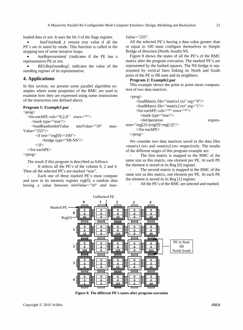
A Massively Parallel Re-Configurable Mesh Computer Emulator: Design, Modeling and Realization
Copyright © 2010 SciRes JSEA
21
loaded data or not. It uses the bit 3 of the flags register. hasFinished( ): returns true value if all the
PE’s are in stand by mode. This function is called in the stopping test of some iterative loops. hasRepresentant( ):indicates if the PE has a
representative PE or not. REGRep[numReg]: indicates the value of the
numReg register of its representative.
4. Applications
In this section, we present some parallel algorithm ex-amples where some properties of the RMC are used to examine how they are expressed using some instructions of the instruction sets defined above.
Program 1: Example1.par <prog> <for-eachPE cols="0,2,4" rows="*"> <mark type="true"/> <loadRandomIntValue minValue="10" max-Value="255"/> <if test="reg[0]>=100"> <bridge type="SB-NS"/> </if> </for-eachPE> </prog>
The result if this program is described as follows: - It selects all the PE’s of the column 0, 2 and 4.
Then all the selected PE’s are marked “true”. - Each one of these marked PE’s must compute
and save in its memory register reg[0], a random data having a value between minValue="10" and max-
Value="255". All the selected PE’s having a data value greater than
or equal to 100 must configure themselves in Simple Bridge of direction (North–South) NS.
Figure 8 shows the states of all the PE’s of the RMC matrix after the program execution. The marked PE’s are represented by the hashed squares. The NS bridge is rep-resented by vertical lines linking its North and South ports of the PE is SB state and its neighbors.
Program 2: Example2.par This example shows the point to point mean computa-
tion of two data matrices.
<prog> <loadMatrix file="matrix1.txt" reg="0"/> <loadMatrix file="matrix2.txt" reg="1"/> <for-eachPE cols="*" rows="*"> <mark type="true"/> <doOperation expres-
sion="reg[2]=(reg[0]+reg[1])"/> </for-eachPE> </prog>
We consider two data matrices saved in the data files «matrix1.txt» and «matrix2.txt» respectively. The results of the different stages of this program example are:
- The first matrix is mapped to the RMC of the same size as this matrix, one element per PE. At each PE the element is stored in its Reg [0] register.
- The second matrix is mapped to the RMC of the same size as this matrix, one element per PE. At each PE the element is stored in its Reg [1] register.
- All the PE’s of the RMC are selected and marked.
Reg[0]
Marked PE
UnMarked PE
PE in State SB
North South
1 2 3 4
0
1
2
3
4
0
43 0 0
000
2300
000
3200
12 0 0
000
13400
000
4500
156 0 0
000
12500
000
22300
6 0 0
000
1200
000
1100
1 0 0
000
10200
000
3400
Figure 8. The different PE’s states after program execution

A Massively Parallel Re-Configurable Mesh Computer Emulator: Design, Modeling and Realization 22
1 2 3 4
0
1
2
3
4
0
43 12 55
101
235
61218
321143
12 12 24
336
1341
135
122
14
11011
20011 211
233100333
12550175
000
2230
223
6 6
12
45559
126
18
101
-125-7
-3 -1 -4
5-15-10
11213
140
14
-330
-33
Reg[2]
Reg[1]
Reg[0]
Figure 9. Result of the point to point sum of two matrices on the modeled RMC
All the marked PE’s execute simultaneously the op-
eration (reg[2]=reg[0]+reg[1]). This is the point to point mean computation. At each PE the result is saved in its reg[0] register.(Figure 9)
Program 3: Example 3.par This example corresponds to an implementation of a
component contour detection of a gray leveled image using Sobel operator. The used image is of size 200 x 200 pixels.
<prog> <for-eachPE rows="*" cols="*"> <mark type="true"/> <loadImage file=”branchng1.jpg” reg=”0” coding=”8”/> <sendAndReceiveData portS="E" regS="0" portR= 'W' regR="1"/> <sendAndReceiveData portS="N" regS="1" portR= 'S' regR="2"/> <sendAndReceiveData portS="W" regS="0" portR= 'E' regR="3"/> <sendAndReceiveData portS="S" regS="3" portR= 'N' regR="4"/> <sendAndReceiveData portS="N" regS="0" portR= 'S' regR="5"/> <sendAndReceiveData portS="W" regS="5" portR= 'E' regR="6"/> <sendAndReceiveData portS="S" regS="0" portR= 'N' regR="7"/> <sendAndReceiveData portS="E" regS="7" portR= 'W' regR="8"/> <doOperation expres-sion="reg[9]=Math.abs(-reg[8]-2*reg[1]-reg[2]+reg[4]+ 2*reg[3]+reg[6])"/> <doOperation expres-sion="reg[10]=Math.abs(reg[8]+2*reg[7]-reg[2]+reg[4]-
2*reg[5]-reg[6])"/> <doOperation expression="reg[1]=reg[9]+reg[10]"/>
</for-eachPE> </prog>
The execution of this program is commented as fol-lows:
- Selecting and marking all the PE’s of the (200 x 200) RMC.
- The image is loaded from file=”branchng1. jpg” and stored in the RMC one pixel per PE. Each PE saves its own gray level pixel (coding=”8”) in its register reg[0].
The following eight “sendAndReceiveData” instruc-tions are used by the PE’s to exchange data between neighboring PE’s, so that each PE will receive its eight neighboring pixel values required by the Sobel operator.
- After the data exchange stage, we compute the absolute values of Gx and Gy of the Sobel operator
- The final result is computed by: expression= "reg[1]=reg[9]+reg[10]"
- The resulted image is located in the RMC, one pixel per PE (i.e. in reg[1] of each PE.), while the input image is still in reg[0].
Figure 10 shows the result of the parallel program of a component contour detection of a gray leveled image using Sobel operator. Each used images is of size 200 x 200 pixels. The images in Figures 10(a), (b) and (c) rep-resenting flower, fishes and a tree branch (respectively) are the input images of the program. The resulted output images are shown in Figures 10(d), (e) and (f).
Program 4: Example 4.par Parallel program of the hierarchical Minimum search
algorithm:
Copyright © 2010 SciRes JSEA
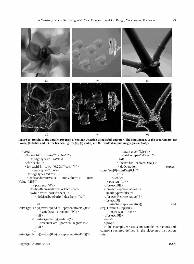
A Massively Parallel Re-Configurable Mesh Computer Emulator: Design, Modeling and Realization 23
(a) (b) (c)
(d) (e) (f)
Figure 10. Results of the parallel program of contour detection using Sobel operator. The input images of the program are: (a) flower, (b) fishes and (c) tree branch, figures (d), (e) and (f) are the resulted output images (respectively)
<prog> <for-eachPE rows="*" cols="*"> <bridge type="SB-WE"/> </for-eachPE> <for-eachPE rows="0,2,3,4" cols="*"> <mark type="true"/> <bridge type="NB"/> <loadRandomIntValue minValue="1" max-
Value="255"/> <push reg="0"/> <defineRepresentativeForEachRow/> <while test="!hasFinished()"> < doDistributeParityIndex from="W"/> <if
test="(getParity()==true)&&(!isRepresentativePE())"> <sendData direction="W"/> </if> <if test="(getParity()==false)"> <receiveData port="E" regR="1"/> </if> <if
test="(getParity()==true)&&(!isRepresentativePE())">
<mark type="false"/> <bridge type="SB-WE"/> </if> <if test="hasReceivedData()"> <doOperation expres-
sion="reg[0]=minReg(0,1)"/> </if> </while> <pop reg="1"/> </for-eachPE> <for-eachRepresentativePE> <mark type="false"/> </for-eachRepresentativePE> <for-eachPE test="hasRepresentative() and
(reg[1]==REGRep[0])"> <mark type="true"/> </for-eachPE> <end/> </prog> In this example, we use some sample instructions and
control structures defined in the elaborated instruction sets.
Copyright © 2010 SciRes JSEA

A Massively Parallel Re-Configurable Mesh Computer Emulator: Design, Modeling and Realization 24
Copyright © 2010 SciRes JSEA
(a) (b)
(c) (d)
Figure 11. Result of a parallel minimum value search algorithm on all the rows of a matrix
This program contains three stages: In the first stage: - All the PE’s are set in Simple Bridge of direc-
tion WE. - All the PE’s of rows 0, 2, 3 and 4 are marked. - Each marked PE computes a random value and
stores it in its register reg[0].
- Finding the representative PE of each row using a macro command <defineRepresentativeForEachRow/>.
The second stage is devoted to a «while» loop, where: 1) The marco command «doDistributeParityIndex
from =‘W’»is used to label the marked PE’s alternatively by 0 or 1.
1 2 3 4
0
1
2
3
4
0
31021
xxx
3 23 x
3 3 x
332x
121231
xxx
12 134 x
12 12 x
1245x
221561
xxx
22 22 x
22 123 x
22223x
111
xxx
1 44 x
1 66 x
155x
12121
xxx
12 101 x
12 134 x
1212x
1 2 3 4
0
1
2
3
4
0
3 3 1
x x x
x x x
x x x
xxx
12 12 1
x x x
x x x
x x x
xxx
22 123 1
x x x
x x x
x x x
xxx
1 55 1
x x x
x x x
x x x
xxx
12 12 1
x x x
x x x
x x x
xxx
1 2 3 4
0
1
2
3
4
0
102 0 1
x x x
23 0 0
3 0 1
3200
123 0 1
x x x
134 0 0
12 0 1
4500
156 0 1
x x x
22 0 0
123 0 1
22300
1 0 1
x x x
44 0 0
66 0 1
5500
12 0 1
x x x
101 0 0
134 0 1
1200
1 2 3 4
0
1
2
3
4
0
23231
xxx
x x x
3 32 1
xxx
1231341
xxx
x x x
12 45 1
xxx
22221
xxx
x x x
123 223 1
xxx
1441
xxx
x x x
55 55 1
xxx
121011
xxx
x x x
12 12 1
xxx
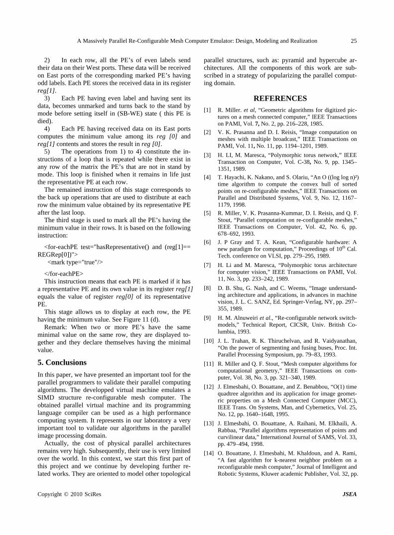
A Massively Parallel Re-Configurable Mesh Computer Emulator: Design, Modeling and Realization 25
2) In each row, all the PE’s of even labels send their data on their West ports. These data will be received on East ports of the corresponding marked PE’s having odd labels. Each PE stores the received data in its register reg[1].
3) Each PE having even label and having sent its data, becomes unmarked and turns back to the stand by mode before setting itself in (SB-WE) state ( this PE is died).
4) Each PE having received data on its East ports computes the minimum value among its reg [0] and reg[1] contents and stores the result in reg [0].
5) The operations from 1) to 4) constitute the in-structions of a loop that is repeated while there exist in any row of the matrix the PE’s that are not in stand by mode. This loop is finished when it remains in life just the representative PE at each row.
The remained instruction of this stage corresponds to the back up operations that are used to distribute at each row the minimum value obtained by its representative PE after the last loop.
The third stage is used to mark all the PE’s having the minimum value in their rows. It is based on the following instruction:
<for-eachPE test="hasRepresentative() and (reg[1]== REGRep[0])">
<mark type="true"/>
</for-eachPE> This instruction means that each PE is marked if it has
a representative PE and its own value in its register reg[1] equals the value of register reg[0] of its representative PE.
This stage allows us to display at each row, the PE having the minimum value. See Figure 11 (d).
Remark: When two or more PE’s have the same minimal value on the same row, they are displayed to-gether and they declare themselves having the minimal value.
5. Conclusions
In this paper, we have presented an important tool for the parallel programmers to validate their parallel computing algorithms. The developped virtual machine emulates a SIMD structure re-configurable mesh computer. The obtained parallel virtual machine and its programming language compiler can be used as a high performance computing system. It represents in our laboratory a very important tool to validate our algorithms in the parallel image processing domain.
Actually, the cost of physical parallel architectures remains very high. Subsequently, their use is very limited over the world. In this context, we start this first part of this project and we continue by developing further re-lated works. They are oriented to model other topological
parallel structures, such as: pyramid and hypercube ar-chitectures. All the components of this work are sub-scribed in a strategy of popularizing the parallel comput-ing domain.
REFERENCES [1] R. Miller. et al, “Geometric algorithms for digitized pic-
tures on a mesh connected computer,” IEEE Transactions on PAMI, Vol. 7, No. 2, pp. 216–228, 1985.
[2] V. K. Prasanna and D. I. Reisis, “Image computation on meshes with multiple broadcast,” IEEE Transactions on PAMI, Vol. 11, No. 11, pp. 1194–1201, 1989.
[3] H. LI, M. Maresca, “Polymorphic torus network,” IEEE Transaction on Computer, Vol. C-38, No. 9, pp. 1345– 1351, 1989.
[4] T. Hayachi, K. Nakano, and S. Olariu, “An O ((log log n)²) time algorithm to compute the convex hull of sorted points on re-configurable meshes,” IEEE Transactions on Parallel and Distributed Systems, Vol. 9, No. 12, 1167– 1179, 1998.
[5] R. Miller, V. K. Prasanna-Kummar, D. I. Reisis, and Q. F. Stout, “Parallel computation on re-configurable meshes,” IEEE Transactions on Computer, Vol. 42, No. 6, pp. 678–692, 1993.
[6] J. P Gray and T. A. Kean, “Configurable hardware: A new paradigm for computation,” Proceedings of 10th Cal. Tech. conference on VLSI, pp. 279–295, 1989.
[7] H. Li and M. Maresca, “Polymorphic torus architecture for computer vision,” IEEE Transactions on PAMI, Vol. 11, No. 3, pp. 233–242, 1989.
[8] D. B. Shu, G. Nash, and C. Weems, “Image understand-ing architecture and applications, in advances in machine vision, J. L. C. SANZ, Ed. Springer-Verlag, NY, pp. 297– 355, 1989.
[9] H. M. Alnuweiri et al., “Re-configurable network switch- models,” Technical Report, CICSR, Univ. British Co-lumbia, 1993.
[10] J. L. Trahan, R. K. Thiruchelvan, and R. Vaidyanathan, “On the power of segmenting and fusing buses, Proc. Int. Parallel Processing Symposium, pp. 79–83, 1993.
[11] R. Miller and Q. F. Stout, “Mesh computer algorithms for computational geometry,” IEEE Transactions on com-puter, Vol. 38, No. 3, pp. 321–340, 1989.
[12] J. Elmesbahi, O. Bouattane, and Z. Benabbou, “O(1) time quadtree algorithm and its application for image geomet-ric properties on a Mesh Connected Computer (MCC), IEEE Trans. On Systems, Man, and Cybernetics, Vol. 25, No. 12, pp. 1640–1648, 1995.
[13] J. Elmesbahi, O. Bouattane, A. Raihani, M. Elkhaili, A. Rabbaa, “Parallel algorithms representation of points and curvilinear data,” International Journal of SAMS, Vol. 33, pp. 479–494, 1998.
[14] O. Bouattane, J. Elmesbahi, M. Khaldoun, and A. Rami, “A fast algorithm for k-nearest neighbor problem on a reconfigurable mesh computer,” Journal of Intelligent and Robotic Systems, Kluwer academic Publisher, Vol. 32, pp.
Copyright © 2010 SciRes JSEA
A Massively Parallel Re-Configurable Mesh Computer Emulator: Design, Modeling and Realization
Copyright © 2010 SciRes JSEA
26
347–360, 2001.
[15] R. Miller et al, “Meshes with re-configurable Buses,” Proceedings of 5th MIT Conference on Advanced Re-search in VLSI, Cambridge, MA, pp. 163–178, 1988.
[16] Ling Tony et al, Efficient parallel processing of image contours,” IEEE Transactions on PAMI, Vol. 15, No. 1, pp. 69–81, 1993.
[17] O. Bouattane, J. Elmesbahi, and A. Rami, “A fast parallel algorithm for convex hull problem of multi-leveled im-ages,” Journal of Intelligent and Robotic Systems, Kluwer academic Publisher, Vol. 33, pp. 285–299, 2002.
[18] A. Errami, M. Khaldoun, J. Elmesbahi, and O. Bouattane, “O(1) time algorithm for structural characterization of multi-leveled images and its applications on a re-config-urable mesh computer,” Journal of Intelligent and Robotic Systems, Springer, Vol. 44, pp. 277–290, 2006.
[19] M. Migliardi and V. Sunderam, “Emulating parallel pro-gramming environments in the harness meta computing system,” Parallel Processing Letters, Vol. 11, No. 2 & 3, pp. 281–295, 2001.
[20] D. Kurzyniec, V. Sunderam, and M. Migliardi, “PVM emulation in the harness metacomputing framework -design and performance evaluation,” Proc. of the Second IEEE International Symposium on Cluster Computing and the Grid (CCGrid), Berlin, Germany, pp. 282–283, May 2002.
[21] M. Migliardi, P. Baglietto, and M. Maresca, “Virtual parallelism allows relaxing the synchronization con-straints of SIMD computing paradigm, Proceedings of HPCN98, Amsterdam (NL), pp. 784–793, April 1998.
[22] M. Migliardi and M. Maresca, “Modeling instruction level parallel architectures efficiency in image processing applications,” Proceedings of of HPCN97, Lecture Notes in Computer Science, Springer Verlag, Vol. 1225, pp. 738–751, 1997.
[23] M. Migliardi and R. Podesta, “Parallel component de-scriptor language: XML based deployment descriptors for grid application components,” Proc. of the 2007 Interna-tional Conference on Parallel and Distributed Processing Techniques and Applications, Las Vegas, Nevada, USA, pp. 955–961, June 2007.

J. Software Engineering & Applications, 2010, 3: 27-33 doi:10.4236/jsea.2010.31003 Published Online January 2010 (http://www.SciRP.org/journal/jsea)
Copyright © 2010 SciRes JSEA
27
Properties of Nash Equilibrium Retail Prices in Contract Model with a Supplier, Multiple Retailers and Price-Dependent Demand
Koichi NAKADE, Satoshi TSUBOUCHI, Ibtinen SEDIRI
Department of Industrial Engineering and Management, Nagoya Institute of Technology, Japan. Email: [email protected], [email protected] Received September 3rd, 2009; revised October 9th, 2009; accepted October 19th, 2009.
ABSTRACT
Recently, price contract models between suppliers and retailers, with stochastic demand have been analyzed based on well-known newsvendor problems. In Bernstein and Federgruen [6], they have analyzed a contract model with single supplier and multiples retailers and price dependent demand, where retailers compete on retail prices. Each retailer decides a number of products he procures from the supplier and his retail price to maximize his own profit. This is achieved after giving the wholesale and buy-back prices, which are determined by the supplier as the supplier’s profit is maximized. Bernstein and Federgruen have proved that the retail prices become a unique Nash equilibrium solution under weak conditions on the price dependent distribution of demand. The authors, however, have not mentioned the numerical values and proprieties on these retail prices, the number of products and their individual and overall profits. In this paper, we analyze the model numerically. We first indicate some numerical problems with respect to theorem of Nash equilibrium solutions, which Bernstein and Federgruen proved, and we show their modified results. Then, we compute numerically Nash equilibrium prices, optimal wholesale and buy-back prices for the supplier’s and retailers’ profits, and supply chain optimal retailers’ prices. We also discuss properties on relation between these values and the demand distribution. Keywords: Supply Chain Management, Nash Equilibrium, Stochastic Demand, Competing Retailers
1. Introduction
Recently, price contract models between suppliers and retailers with stochastic demand have been analyzed based on well-known newsvendor problems. Cachon [1] has reviewed models with one supplier and one retailer under several types of contracts. In a market, however, many retailers exist and they compete in order to attract the maximum number of consumers. In this context, Yano and Gilbert [2] have been interesting in contracting models in which the demand is stochastic and depends on price. Wang et al. [3] and Petruzzi [4] have studied de-centralized price setting newsvendor problems under multiplicative retail demand functions. Song et al. [5] have analyzed theoretically the optimal prices and the fraction of a total profit under individual optimization to that under supply chain optimization.
In Bernstein and Federgruen [6], they have analyzed a contract model with single supplier and multiple retailers and price dependent demand, where retailers compete on retail prices. Each retailer decides a number of products
he procures from the supplier and his retail price to maximize his own profit. This is achieved after giving the wholesale and buy-back prices, which are determined by the supplier as the supplier’s profit is maximized. They have proved that the retail prices become a unique Nash equilibrium solution under weak conditions on the price dependent distribution of demand. They, however, have not mentioned the numerical values and properties on these retail prices, the number of products and their individual and overall profits.
In this paper, we analyze the model numerically. We first indicate some numerical problems with respect to the theorem of Nash equilibrium solutions, which Bern-stein and Federgruen [6] proved, and we show their modified results. Then we present Nash equilibrium prices, optimal wholesale and buy-back prices for the supplier’s and retailers’ profits, and optimal retail prices under supply chain optimization, analytically and nu-merically. We also discuss the properties on a relation-ship between these values and the demand distribution.
In the next section, we present the competing retailers

Properties of Nash Equilibrium Retail Prices in Contract Model with a Supplier, Multiple Retailers and Price-Dependent Demand 28
model introduced in [6], and we discuss the sufficient conditions on the existence and the uniqueness of the Nash solution. In Section 3 we investigate the model with exponential and uniform distribution functions and with linear and Logit demand functions. In Section 4, we present numerical results and discuss the behavior of Nash equilibrium solutions and properties of the profits and prices.
2. Competing Retailers’ Model
The model of competing retailers for one supplier and retailer introduced in [6], is shown
in Figure 1.
SN , 1iR i N
This model is set under wholesale and buyback pay-ment scheme. The supplier incurs retailer S , 1iR
a wholesale price for each product, com-
bined with an agreement to buyback unsold inventory at . We assume that the supplier has ample capacity to
satisfy any retailer demand and produce products at a constant production cost rate , which includes the
transportation cost to retailer . When and are
given, each retailer orders his quantity and cho-
oses his retail price . A salvage rate is
adopted in the supply chain. To avoid trivial setting, the model parameters are chosen as and
i N
ib
i
c
iR
w
i
iw
iw
ib
ii cv
iR
ipiy
iv
i iv b
for . 1 i N The demand is random and depends on the
price vector , with a cumulative dis-
tribution function . It is restrained to a
multiplicative form
i
p p ,
G (x
D (p)
1 2 Np , , p
i 1| p ,..., p
( )iD p d
i
N )
( )i p , where i is a
random variable with a cumulative distribution function
S
R1
R2
Ri
RN
ci
vi
w1
b1 w2
b2
wi
bi wN
bN
p1
p2
pi
pN
Figure 1. Competing retailers’ model
iG (.) and a probability density function ig (.) . In addi-
tion i is assumed to be positive only on x
and independent of the price vector p. This
implies that
min[ ,ix xmax ]i
i ii
xG (x|p) G
d (p)
.
The demand function depends on the whole
price vector. It is supposed that decreases in pi-
and increases in pj for all j≠ i, 1 ≤ I ≤ N, that is
( )id p
( )id p
0
i
i
p
pdand
0
j
i
p
pd.
Let 1 2, , , Ny y y y denotes the order vector of
the model. The expected profit function for the retailer is given by iR
( , ) min , ( ) ( )i i i i i i ip y p E y D p b E y D p w y i i
,
where . It can be rewritten as max 0,a a
)()()(),( pDyEbpywpyp iiiiiiii (1)
From (1), the retail prices p impact on the profits of all retailers and his order quantity, however, affects only his own profit. In addition the retailer wants to maximize his order quantity. Then, the derivation of the retailer i’s profit function given by Equation (1) on is equal to
zero iy
0
i
i
y
)y,p( (2)
Therefore, the retailer i's optimal corresponding order can be obtained from (1) and (2) by
ii
iiiii bp
wpG)p(d)p(y 1 (3)
This result reduces the no-cooperative game in the (p, y)-space to a p-space game. In this space the retailers compete only on prices (reduced retailer game). Then, considering the Equations (1) and (3), we get the retailers profits as a function of p only, as
1
1
i ii i i i i
i i
i ii i i i
i i
p w(p) d (p) (p w )G
p b
p w(p b )E G
p b
det ( | ) ( ( ))i i i i ip w L f p (4)
where is the profit function
with a deterministic demand ( )p ,
det ( | ) ( ) ( )i i i i ip w p w d p
i iy d( )
( )( )
i ii i
i i
p wf p
p b
Copyright © 2010 SciRes JSEA

Properties of Nash Equilibrium Retail Prices in Contract Model with a Supplier, Multiple Retailers and Price-Dependent Demand 29
is the critical fractile, and
i
We define and we apply
the logarithm
(S’), as 1 ( ( ))1 1 1( ) ( ) ( ) ( ) /
i i iG f p
i i i i i i i iL f G f f E G f ug u du f
1 ( ( ))ˆ ( ) ( )i i iG f p
i i iL p ug u du
to (4), we get for 1 i N
log ogi i i iπ (p) L (p )log log li i(p b ) d (p)
(5)
The supplier profit function is given by
( ) ( ) ( )N
M i i i i i i iw c y b E y D p1i
. Using
Equation (3), it can be expressed as
1M
1i i i i
i
d p w c G
1 ( ) .
Ni i
i i
i ii i i i
i i
p w
p b
p wb v E G
p b
(6)
Differentiating (5) on for ip Ni 1
),p(Up)p(dp ii
iii )p(d)p(~log ii
1 with
1 (i iG f
2
( ) )1( )
( ) ( )i i i
i ii i i i i i
w b pU p
p b p b L p
(7)
Bernstein and Federgruen [6] have proved tistence of a Nash solution for the reduced retailer
ga
the same re each reta price clos interval
o hold:
hat the ex-*p
me is assured by the following condition (A). (A): For each {1,..., }i N the function log ( )id p is
increasing in ( , )i jp p for all i j .
,
It is assumed in ference [6] that iler
iR chooses his ip from a edmin max,i ip p . The authors proved the uniqueness of the
max
Na
sh solution in the price space
min max, 2 ,i iiiw b p . This has provided the
following conditions (D) and (S) t
(D):
p
2 det 2 det
2
log ( |i i i
j ii
p w b
p
log ( | ) )i i i
i j
p w b
p p
,
(S):
x
iii
ii x)x(Gdu)u(ug
)x(g
)x(Gx)x( 02 2ψ ,
for a anll is the medi
of the on under the
{1,..., }i N distribution G
onditions ma
i
, where imx
i ). However, th
n the b
( im
e soluti
ndabove c y exist o ou ary of the area
i
ii pbwp maxmin ,2,max . In this case, it does not
satisfy log ( )0.i p
ip
the condition (S) is modified to
(S’):
2( )( ) ( ) 0
( )i x
ix
ug u du G x x( ) 2i ii
Gx x
g x
] Then, the following theorem can
ained. S’) hold, th um prices on
ψ
for all min max[ ,i ix x x .
be obtThe enorem : If conditions (A), (D) and (
there is a unique set of Nash equilibri
[ , )ii
w w tisfy hich salog ( )
0i p
for all
i
{1,..., }i N
p .
Proof: In the same way as in B nd Federgruen s a unique Nash s [ , )iw
ernstein a[6], there i olution in *p
i
which satisfies , because *i ip w for each {1,..., }i N ,
( ) 0i p when i ip w whereas ( ) 0i p when
i ip w . This im s that plielog ( )
i
p
p
0i
when
*p p for all i N{1,..., } .
following, the retailers t these um prices, whereas the s the be-
retailers and dek prices t
In the sell products aequilibri upplier knows havior of the termines the wholesale and buybac o maximize his own profit. This system is
faces a random de-
called “individual optimization”. On the other hand, the problem of determining retail prices and quantities of products to maximize the entire profits of supply chain is called “supply chain optimization”
3. Determination of the Nash Equilibrium
As shown in Figure 2, we study a two competing retail-ers’ model. Each retailer {1, 2}i
mand ( ),iD p where 1 2( , )p p p . We assume two
types of cumulative distribution functions of demand. We consider first the exponential case and then the uni-form one.
3.1 Exponential Case
The cumulative distribution function in the exponential
S
R1 ci w1 1
R2
b1 w2
b2
p
p2 vi
Figure 2. Two competing retailers’ model
Copyright © 2010 SciRes JSEA

Properties of Nash Equilibrium Retail Prices in Contract Model with a Supplier, Multiple Retailers and Price-Dependent Demand 30
( ) 1 xiG x e for all 0x , case is given by
where iE is set as
rse function of
0 1y . Wit
one without loss
( )iG x is given by
h
of generality. The 1( ) log(1 )iG y y inve
for all ( )
( )i i
i i
, we get ( )i if p
p w
p b
)bp
bw()bw(wp
bp)p(L
iiii
iiiiiiii log
1
Then, using (7), we obtain
log
i ii i
i ii i i i
i
p wU (p )
wp b w
b
i ii
bp w b
p
1) Linear demand function The linear demand is given for by
j
, , {1, 2}j i i j
( )i i i i ijj i
d p p p
with 0,,0 ijii .(8)
we obtain the system of equations
With this demand function,
1 11 1
1 1 1 1 12 2
2log ( )p 2
2 221 1
log ( )( ) 0,
( ) 0.
pU p
p p p
U pp
It can be rewritten as
2 2 2 2p p
2 2 2 2 2 2 2 21
( ) ( ),
( )
U p p U pp
U p
21 2 2
1 1 1 1 1 1 1 12
12 1 1
( ) ( ).
( )
U p p U pp
U p
(9)
The optimal order quantities and can be
evaluated to 1y 2y
1 11 1 1( )y p
1 12 2
1 1
2 22 2 2 2 21 1
log ,
( ) log
p bp p
w b
p by p p p
w
Since
2 2
.b
1 log ,i i i i ii
p w p b w pE G
p
i
ii i i i i ib w b p b
from (6), the supplier profit function can be expressed as
2
M1
log i i i ii i i i i i
i i i i i
p b p wd p w c b b
w b p b
1 11 1 1 11 1
1 1
2 22 2 2 22 2
2 2
log ,
log
p bp d p b w p w
w b
p bp d p b w p w
w b
2) Logit demand function Now, the problem is studied with a logistic demand
function, expressed by
2( )
ipi
i
1
jp
i jj
C k e
k ed p
for 0and ii k,C, . (10)
With this demand function we obtain the system of equations
2
1 2
1
1 2
1 1 21 1
1 1 1 2
2 2 12 2
2 2 1 2
log ( ) ( )( ) 0,
log ( ) ( )( ) 0.
p
p p
p
p p
p C k eU p
p C k e k e
p C k eU p
p C k e k e
Then, we have
22 2 2 2 2 2 2
1
( ) ( )1log ,
pC C U p k e U pp
1
1 2 2
1 1 1 1 12
2 1 1
( )
( )1log
( )
p
k U p
C C U p k e U pp
k U p
1 1( )
.
The order quantities are given by
1
1 2
2
1 2
1 11
1 11 1 2
2 22
2 22 1 2
1
2
) log ,
( ) log .
p p
p
p p
k e p b
w bC k e k e
k e p by p
w bC k e k e
The supplier profit function and retailers’ profit func-tio in the same way as for the linear de-ma
3.2 Uniform Case
The cumulative distribution function in the uniform ase is given by
(p
y p
ns are obtainednd function.
c
(1 )( ) ,
2i
ii
G xa
1 1 ,0 1, 1,2,i i i
x a
a x a a i
where
1.iE 1( ) 1G y
( i
The inverse function of is g ven
by i for . With
( )iG x
0 1y
i
.
The retailers’ profit functions are given by
2i ia a y ( ) ) / ( )i i ii if p p w p b , we get
( ) 1i i i ii i i i
i i i i
p w p wL p a a
p b p b
Copyright © 2010 SciRes JSEA

Properties of Nash Equilibrium Retail Prices in Contract Model with a Supplier, Multiple Retailers and Price-Dependent Demand
Copyright © 2010 SciRes JSEA
31
r {1, 2}i Then by (7) fo
1 21
( ) 1
1
i ii i
i i i i i ii i
p w
p b p w p wa a
p b
1) Linear demand function With the linear demand given by (8) and , we
i ii ii i
a ap bw b
U p
i i
)p(U ii
obtain
2 2 2 2 2 2 2 (
)
U p 21
21 2 2
1 1 1 1 1 1 1 12
12 1 1
( ) ),
(
( ) ( ).
( )
U p pp
U p
U p p U pp
U p
r quantities are given by The optimal orde
1 11 1 1 1 12 2 1 1
1 1
2 22 2 2 2 21 1 2 2
2 2
( ) 1 2 ,
( ) 1 2 .
p wy p p p a a
p b
p wy p p p a a
p b
equal to The supplier profit function is
2
M
p
1
2
1 2 i ii i i i i i
i i i
i ii i
i i
wd p w c a a
p b
p wa b
p b
.
The retailers’ profit functions are given by
1 11 1 1 1
1 1
1 1 2
1 11 1 1
1 1
2 22
2 2
2 2 2
2 22 2 2
2 2
1 2
,
.
p w a ap b
p d pp w
a p bp b
p w
p bp d p
p wa p b
p b
2) Logit demand function With the Logit function given by (10), we obtain and as
2 2 21 2p w a a
p w
1p 2p
2
1
2 2 2 2 2 2 21
1 2 2
1 1 1 1 1 1 12
2 1 1
1log ,
1log .
λpλC C U (p ) k e U
λp
(p )p
λ k λ U (p )
λC C U (p ) k e U (p )p
λ k λ U (p )
The optimal order quantities are given by
1
1 2
2
1 2
1 11 1
1 11 1 2
2 22 2
2 22 1 2
( ) 1 2 ,
( ) 1 2 .
p
p p
p
p p
k e p wy p a a
p bC k e k e
k e p wy p a a
p bC k e k e
11
22
The supplier profit function and retailers’ profit func-tions are obtained in the same way as for the linear de-mand function.
3. zation
Wan ord antities to maximize the overall profit of the supply chain, the wholesale and buyback prices are meaningless because they are payments between the supplier and the retailers. As the whole of the supply chain is equivalent to a single retailer with whoprice and buyback
3 Supply Chain Optimi
hen the supplier and the retailers determine the prices d the er qu
lesale
1 2( , )c c 1 2( , ) , and by using (3),
the optimal order quantity (the amount of products) is
given by 1( ) ( )I i ii i i
p cy p d p G
i ip
. By u
sing (4), the
overall expected profit of the supply chain is
2
1( ) ( ) ( )I i i
i i i ii i i
p cp p c d p L
p v
, (11)
wh ere, the retail prices 1 2( , )p p are given. The optimal
retail prices 1 2( , )I Ip p in the integrated supply chain
maximize the profit function given by (11).
ote th
4. Numerical Examples
4.1 Geometric Analysis of the Nash Solution
The system of equations on 1 2( , )p p that solves the
profit functions for the two retailers is obtained in Section
3. In the case of exponential demand and linear functions,
we den e right hand sides of two equations in (9) by
2 2( )f p and 1 1( )f p , respectively. Then the equations
(9 e ) becom 1 2 ( )p f 2p and Note that in
s sa2 1( ).p f p
tisfied 1
other case by ( , )p p form
1 2 2( )p f p
the equations 1 2
and 2 1 1( )p f p similarly. Geom
he
etrically,
Nash to analyze theution, we
behavior ot the f
of thncti
e system around tons ( )i isol pl u f p fo
le solutions fo solution
r 1p and 2p
r the equa-in Figure 3. There are multipe Nashtions, but there is a uniqu 1 2( , )p p with
( 1, 2)i ip w i , which has been proved in the theorem
of Section 2.
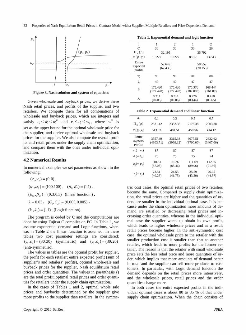
Properties of Nash Equilibrium Retail Prices in Contract Model with a Supplier, Multiple Retailers and Price-Dependent Demand32
P1
P2
w2
w1
1 2( , )p p
Figure 3. Nash solution and system of equations
Given wholesale and buyback prices, we derive these Nash retail prices, and profits of the supplier and two retailers. We compute them for all combinations of wholesale and buyback prices, which are integers and satisfy and i
Ui i ic w w i iv b w , where is
set as the upper bound for the optimal wholesale price for the supplier, and derive optimal wholesale and buyback prices for the supplier. We also compute the overall prof-its and retail prices under the supply chain optimization, and compare them with the ones under individual i-mization.
.2 Numerical Results
Uiw
opt
4
In numerical examples we set parameters as shown in the following:
1 2( , ) (0,0) ,
1 2( , )) (100,100 , 1 2( , ) (1,1) ,
12 21( , ) (0.3,0.3) (linear function ) ,
0.03 , 1 2( , ) (0.005,0.005)C C ,
1 2( , ) (1,1)k k , (Logit function).
The program is coded by C and the computations are mpiler on PC. In Table 1, we
d Logit functions, wher-
cost parameter settings are considered: etric) and
done by using Fujitsu C coassume exponential demand aneas in Table 2 the linear function is assumed. In these tables two
1 2( , ) (30,30)c c (symm 1 2( , ) (30, 20)c c
(anti-symmetiric). The values in tables are the optimal p for supplier,
the profit for each retai m of supplier’s and retailers’ profits), optimal whole-sale and buyback prices for the supplier, Nash ilibrium retail prices and order es in paranthesis () are th
function
i
rofit ler; entire expected profit (su
equ quantities. The valu
e total profit, optimal retail prices and order quanti-ties for retailers under the supply chain optimization.
In the cases of Tables 1 and 2, optimal whole sale prices and buybacks determined by the supplier give more profits to the supplier than retailers. In the symme-
Table 1. Exponential demand and logit
1 2 1 2 Ci 30 30 30 20 ( )M p 32.195 35.792
( , )i i ip y 10.227 10.227 7 3.843
Entire expected profits
52.649 (62.430)
58.552 (7
8.91 1
0.153)
iw 98 98 100 88
ib 47 47 47 47
175.420 (172.428)
175.420 (172.428)
175.376 (182.095)
168.444 (161.07)
0.311 0.311 0.276 0.418
ip
iy (0.606) (0.606) (0.444) (0.965)
ential demand and linear function Table 2. Expon
ia 0.1 0.3 0.5 0.7
( )M p 2531.42 2352.36 2176.38 2003.38
( , )i i ip y 513.03 481.51 450.56 414.12
Entire expected profits
3557.49 (4303.71)
3315.38 (3999.12)
3077.51 (3700.00)
2832.62 (3407.00)
1 2( )w w 87 87 87 87
1 2( )b b 75 75 75 74
1( )2p p 110.31 110.97 111.69 112.55 ) (87.08) (88.46) (89.96) (91.56
2 (4 )
2 (4 )
2 (4 )
2 (4 ) 1 2( )y y 3.51
0.264.551.75
5.593.20
6.054.57
tric cost cases ptim il pr f two retailers bec same. red to supply ptimiza-tio ail pric gher and the s of or-ders are smaller in the individual optimal case. It is be-cause u er the n opti ation m amount f de-mand a satisf dec sing re prices in-creasing orde ies s i div ti-mal case the r o o fit, which leads to er w le pr nd a sult retail prices b ig he mm ost ase, the optimal wholesale price to the retailer with the
smal ther retailer, which leads to m rofits he fo -tailer. The reaso that th ailer w mall wprice sets he il d m nt r-der, which im at m ou ur in t d the supplier can sell more products to cus-tom pa w it he dem epe th ri ly, and the wholes prices tail pri nd thquantities chang ore.
In both cases entire pected profits in indi-vidual optimal is a 0 to of er supply chain o n t n c of
, the o al reta ices oome the
n, the retCompa chain oes are hi quantitie
nd chai miz ore s ore ied by rea tail and r quantit , wherea n the in idual op
supplie wants to btain its wn pro high holesa ices a s a re
ecome h her. In t anti-sy etric cc
ler production cost is smaller than that to anoore pe ret
for tith s
rmer reholesale n is
t less reta price an ore qua ities of oplies th ore am nts of demand occ
otal aners. In and d
rticular, ith Log demand function tnds on e retail p ces more intensive
ale , re ces a e order e m the ex the
cases bout 8 85 % that undoptimizati n. Whe he chai onsists
Copyright © 2010 SciRes JSEA
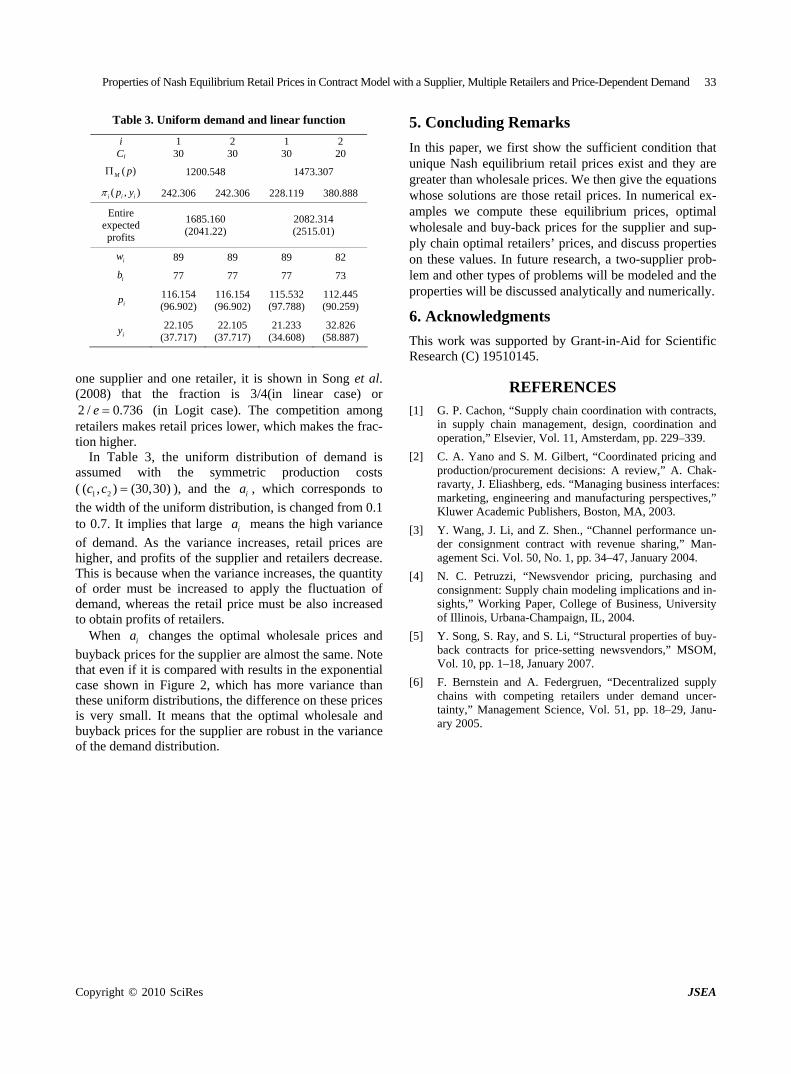
Properties of Nash Equilibrium Retail Prices in Contract Model with a Supplier, Multiple Retailers and Price-Dependent Demand
Copyright © 2010 SciRes JSEA
33
Table 3. Uniform de and unct
i
mand linear f ion
1 2 1 2 Ci 30 30 30 20
( )M p 1200.548 1473.307
( , )i i ip y 242.306 242.306 228.119 380.888
Entire expected profits
1685.160 (2041.22)
2082.314 (2515.01)
iw 89 89 89 82
ib 77 77 77 73
ip 116.154 (96.902)
116.154 (96.902)
115.532 (97.788)
112.445(90.259)
iy 22.105 (37.717)
22.105 (37.717)
21.233 (34.608)
32.826 (58.887)
one supplier and one retailer, it is shown in Song et al. (2008) that the fraction is 3/4(in linear case) or 2 / 0.736e (in Logit case). The competition among retailers makes retail prices lower, which makes the frac-tion higher.
In Table 3, the uniform distribution of demand is assumed with the symmetric production costs ( ( 1 2, ) (30,30)c c ), and the ia , which corresponds to
the width of the uniform distribution, is changed from 0.1 to 0.7. It implies that large ia means the high variance
of dem s are higher, d profits f the su lier and tailers d rease. This is because when the va ce inc es, the antity of order m t be in to apply t ation of demand, whereas the lso inc d to obtain pro its le
W changes the optimal wholesale prices an
buyb es for t r are almo e. Notethat even it is c ared w result the exponentialcase shown in Fig e 2, whi h has m variancethese unif dist tions, difference on theis very small. o h and buyback prices e t nceof the demand d
tail prices. In numerical ex-am
rant-in-Aid for Scientific
t with revenue sharing,” Man-
hain modeling implications and in-sights,” Work usiness, University of Illinois, Urb 4.
5. Concluding Remarks
In this paper, we first show the sufficient condition that unique Nash equilibrium retail prices exist and they are greater than wholesale prices. We then give the equations whose solutions are those re
ples we compute these equilibrium prices, optimal wholesale and buy-back prices for the supplier and sup-ply chain optimal retailers’ prices, and discuss properties on these values. In future research, a two-supplier prob-lem and other types of problems will be modeled and the properties will be discussed analytically and numerically.
6. Acknowledgments
This work was supported by GResearch (C) 19510145.
REFERENCES [1] G. P. Cachon, “Supply chain coordination with contracts,
in supply chain management, design, coordination and operation,” Elsevier, Vol. 11, Amsterdam, pp. 229–339.
[2] C. A. Yano and S. M. Gilbert, “Coordinated pricing and production/procurement decisions: A review,” A. Chak-ravarty, J. Eliashberg, eds. “Managing business interfaces:marketing, engineering and manufacturing perspectives,” Kluwer Academic Publishers, Boston, MA, 2003.
., “Channel performance un-[3] Y. Wang, J. Li, and Z. Shender consignment contracand. As the variance increases, retail price
an o pp re ecrian reas qu
us creased he fluctu retail
of retaiprice m
rs. ust be a rease
fhen ia
ack pric
agement Sci. Vol. 50, No. 1, pp. 34–47, January 2004.
[4] N. C. Petruzzi, “Newsvendor pricing, purchasing and consignment: Supply c
ing Paper, College of Bana-Champaign, IL, 200
d
[5] Y. Song, S. Ray, and S. Li, “Structural properties of buy-back contracts for price-setting newsvendors,” MSOM, Vol. 10, pp. 1–18, January 2007.
he supplie st the sam if omp ith s in
urribu
c the
ore than
[6] F. Bernstein and A. Federgruen, “Decentralized supply chains with competing retailers under demand uncer-tainty,” Management Science, Vol. 51, pp. 18–29, Janu-ary 2005.
orm se prices It means that the ptimal w olesale for the supplier ar robust in he variaistribution.

J. Software Engineering & Applications, 2010, 3: 34-38 doi:10.4236/jsea.2010.31004 Published Online January 2010 (http://www.SciRP.org/journal/jsea)
Copyright © 2010 SciRes JSEA
A Polar Coordinate System Based Grid Algorithm for Star Identification
Hua ZHANG1, Hongshi SANG1*, Xubang SHEN2
National Key Laboratory of Science and Technology on Multispectral Information Processing technologies, Huazhong University of Science and Technology, Wuhan, China; 2Xi’an Microelectronics Technology Institute, Xi’an, China. Email: [email protected], [email protected] Received September 3rd, 2009; revised September 28th, 2009; accepted October 6th, 2009.
ABSTRACT
In Cartesian coordinate systems, the angular separation-based star identification algorithms involve much trigon- ometric function computing. That delays the algorithm process. As in a polar coordinate system, the coordinates are denoted by angular values, it is potential to speed up the star identification process by adopting a polar coordinate sys-tem. An angular polar coordinate system is introduced and a grid algorithm based on the coordinate system is proposed to enhance the performances of the star identification process. The simulations demonstrate that the algorithm in the angular polar coordinate system is superior to the grid algorithm in the rectangle Cartesian coordinate system in com-puting cost and identification rate. It can be used in the star sensors for high precision and high reliability in spacecraft navigation. Keywords: Star Identification, Grid Algorithm, Polar Coordinate System, Star Sensor
1. Introduction
As the star sensors are used widely in autonomous spacecraft navigation, the star identification algorithm must be of time efficiency and high identification rate. Most star identification algorithms employ the angular star pair distance or polygon to build the guide database. These algorithms include polygon match algorithm, tri-angle algorithm [1–4] and group match algorithm [5–7], etc. Another class of star identification algorithms ac-complishes star identification in terms of pattern recogni-tion or best match. These algorithms associate each star with a pattern or signature determined by its surrounding star field. Then the star identification process can be treated as finding the closest match between the observed patterns and the catalog patterns. The most representative algorithm in this class is grid algorithm [8]. Compared with other algorithms, grid algorithm is an excellent al-gorithm with a higher identification rate and smaller memory requirement, as well as it is computationally efficient [9]. However, this algorithm needs to find the closest neighboring star of the reference star to generate a star pattern. As many fixed stars are variable in visual brightness and the measuring noises exist in measure-ment, the identification probability for the closest neighboring star is comparatively low. That leads to identification failure resulting from misidentifications.
The literature [10] proposes a new grid algorithm adopt-ing the radial and cyclic features of the stars in star iden-tification. The algorithm demonstrates excellent per-formance in identification rate.
Recently, almost all the star identification algorithms are based on the Cartesian coordinate system. Imper-fectly, the angular separations must be computed by us-ing trigonometric functions. That delays the star identi- fication process. As is known, the polar coordinate system involves the angular information in the coor- dinates. It is potential to improve the star identification algorithm in the round polar coordinate system. In this paper, an angular polar coordinate system is proposed for the star sensor and a grid algorithm in the proposed polar coordinate system is introduced. In the simulations, the algorithm proposed is compared with the grid algorithm in the Cartesian coordinate system introduced in the literature [10]. As the simulations demonstrate, the algorithm in the angular polar coordinate system is superior to that in the Cartesian coordinate system.
The paper is separated into four major sections as fol-lows: the angular polar coordinate system for the star sensor is introduced in the second section, and the grid algorithm for star identification in the angular polar co-ordinate system is introduced in the third section. In the last two sections, the simulations are presented and the results are discussed.

A Polar Coordinate System Based Grid Algorithm for Star Identification 35
2. Angular Polar Coordinate System for Star Sensor
The polar coordinate system is well known and used widely. The proposed coordinate system is derived from the conventional polar coordinate system to be used in focal length related image processing field, in that the radial coordinate is denoted by an angular value, so named angular polar coordinate system. As shown in Figure 1, the radial coordinate is denoted by φ, which is the view angle from the focus of the lens physically. And the angular coordinate is denoted by θ, just the same as the angular coordinate in the conventional polar coordi-nate system [11]. The coordinate angles in the polar no- tation are expressed in either degrees or radians (2π rad being equal to 360°), and the angular coordinate θ is measured counterclockwise from the axis and limited to be non-negative values. The axis for 0 is chosen to be the same as the direction of the X axis of the image sensor in the Cartesian coordinate system. Then the two polar coordinates φ and θ can be converted to the Cartesian coordinates x and y by using the trigonometric functions,
tan cos
tan sin
x f
y f (1)
where f is the focal length of the sensor lens. In the Cartesian coordinate system, if the coordinates
of the two stars in the planar frame of the star sensor are ( , ) and ( , ), the two unit vectors below can de-
note the stars in the body coordinate of the star sensor, ix iy jx jy
2 2 2 2 2 2
1 1
ji
i i j
i i j j
j
xx
v y vx y f x y ff
y
f
,
(2)
where f denotes the focal length of the optical lens in the star sensor. Then the angle between the two vectors can be computed,
arccos( ) ij i je v v (3)
In star identification process, the two stars are called a star pair, and the angle between the two stars is called the angular separation or angular distance between the star pair. The principle of angular separation matching is that the angular separations between the star pairs in the star image are computed and compared with those stored in the guiding catalog. If the differences is within an error bound on the expected errors, the angular separation pat-tern is considered matched and the stars made up of the star pair can be determined.
While in the angular polar coordinate system, if one star is located at the polar point, the radial coordinate of another star is just the angular separation between the two stars. And the angular coordinate can represent the distribution of the star relatively, as shown in Figure 2. Therefore, it is potential to use the angular polar coordi-nate system for star identification to avoid computing the angular separations.
In the polar coordinate system, the polar grids are used. As shown in Figure 2, the planar image frame is divided into mean radial and cyclic angular grids. In both coor-dinate directions, the frame can be divided by mean an-gular distance. The distribution of the stars in the frame can be denoted by the angular grids. We use the concepts of the radial and cyclic feature in the literature [10] and realize a grid algorithm for star identification in the an-gular polar coordinate system to improve the perform-ance of the algorithm.
3. Star Identification Algorithm in the Polar Coordinate System
The concept of the algorithm we propose is to implement fast coarse star identification by using the distribution of the observed stars in the FOV (field of view) of the star-
φ
φ
φ
Figure 1. Angular polar coordinate system for star sensor
Copyright © 2010 SciRes JSEA
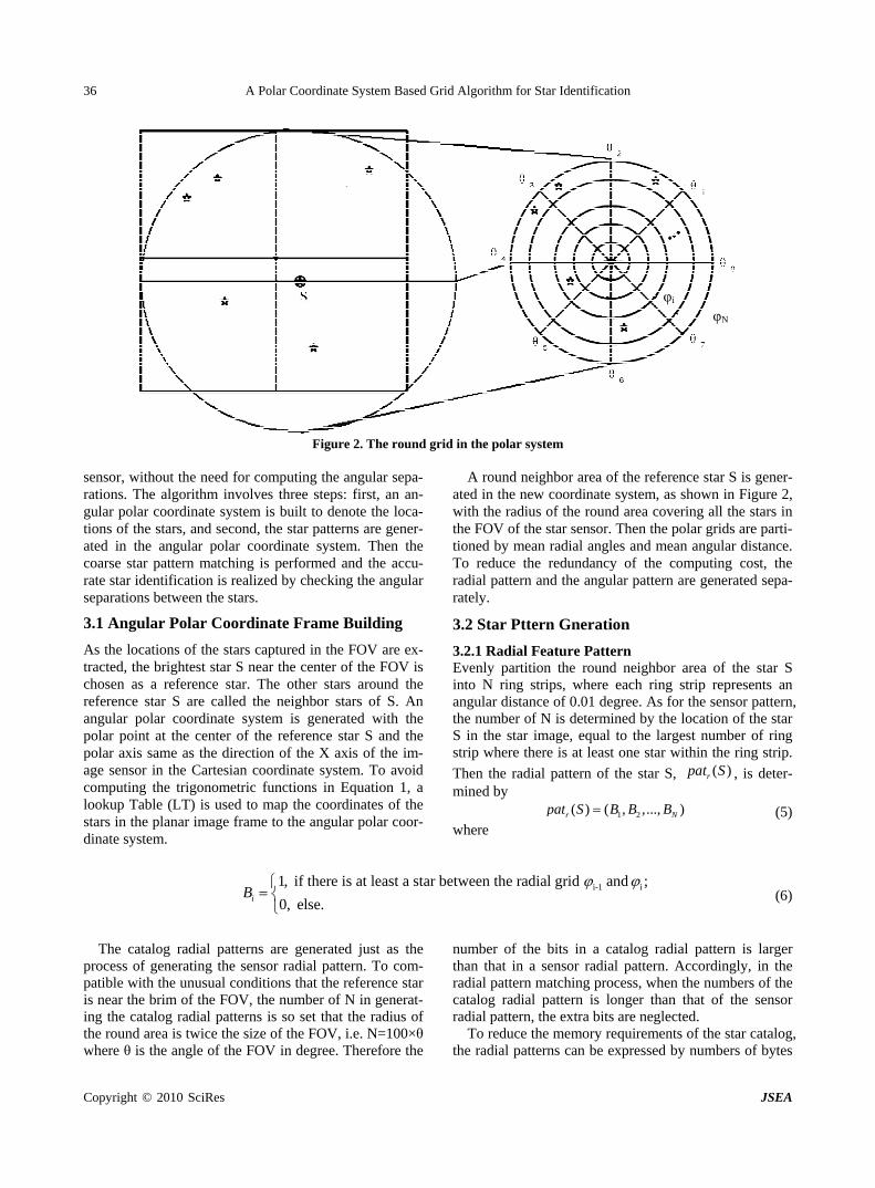
A Polar Coordinate System Based Grid Algorithm for Star Identification 36
φi φN
Figure 2. The round grid in the polar system
sensor, without the need for computing the angular sepa-rations. The algorithm involves three steps: first, an an-gular polar coordinate system is built to denote the loca-tions of the stars, and second, the star patterns are gener-ated in the angular polar coordinate system. Then the coarse star pattern matching is performed and the accu-rate star identification is realized by checking the angular separations between the stars.
3.1 Angular Polar Coordinate Frame Building
As the locations of the stars captured in the FOV are ex-tracted, the brightest star S near the center of the FOV is chosen as a reference star. The other stars around the reference star S are called the neighbor stars of S. An angular polar coordinate system is generated with the polar point at the center of the reference star S and the polar axis same as the direction of the X axis of the im-age sensor in the Cartesian coordinate system. To avoid computing the trigonometric functions in Equation 1, a lookup Table (LT) is used to map the coordinates of the stars in the planar image frame to the angular polar coor-dinate system.
A round neighbor area of the reference star S is gener-ated in the new coordinate system, as shown in Figure 2, with the radius of the round area covering all the stars in the FOV of the star sensor. Then the polar grids are parti-tioned by mean radial angles and mean angular distance. To reduce the redundancy of the computing cost, the radial pattern and the angular pattern are generated sepa-rately.
3.2 Star Pttern Gneration
3.2.1 Radial Feature Pattern Evenly partition the round neighbor area of the star S into N ring strips, where each ring strip represents an angular distance of 0.01 degree. As for the sensor pattern, the number of N is determined by the location of the star S in the star image, equal to the largest number of ring strip where there is at least one star within the ring strip.
Then the radial pattern of the star S, , is deter-mined by
( )rpat S
1 2( ) ( , ,..., )r Npat S B B B (5) where
i-1 i1, if there is at least a star between the radial grid and ;
0, else.iB
(6)
The catalog radial patterns are generated just as the process of generating the sensor radial pattern. To com-patible with the unusual conditions that the reference star is near the brim of the FOV, the number of N in generat-ing the catalog radial patterns is so set that the radius of the round area is twice the size of the FOV, i.e. N=100×θ where θ is the angle of the FOV in degree. Therefore the
number of the bits in a catalog radial pattern is larger than that in a sensor radial pattern. Accordingly, in the radial pattern matching process, when the numbers of the catalog radial pattern is longer than that of the sensor radial pattern, the extra bits are neglected.
To reduce the memory requirements of the star catalog, the radial patterns can be expressed by numbers of bytes
Copyright © 2010 SciRes JSEA
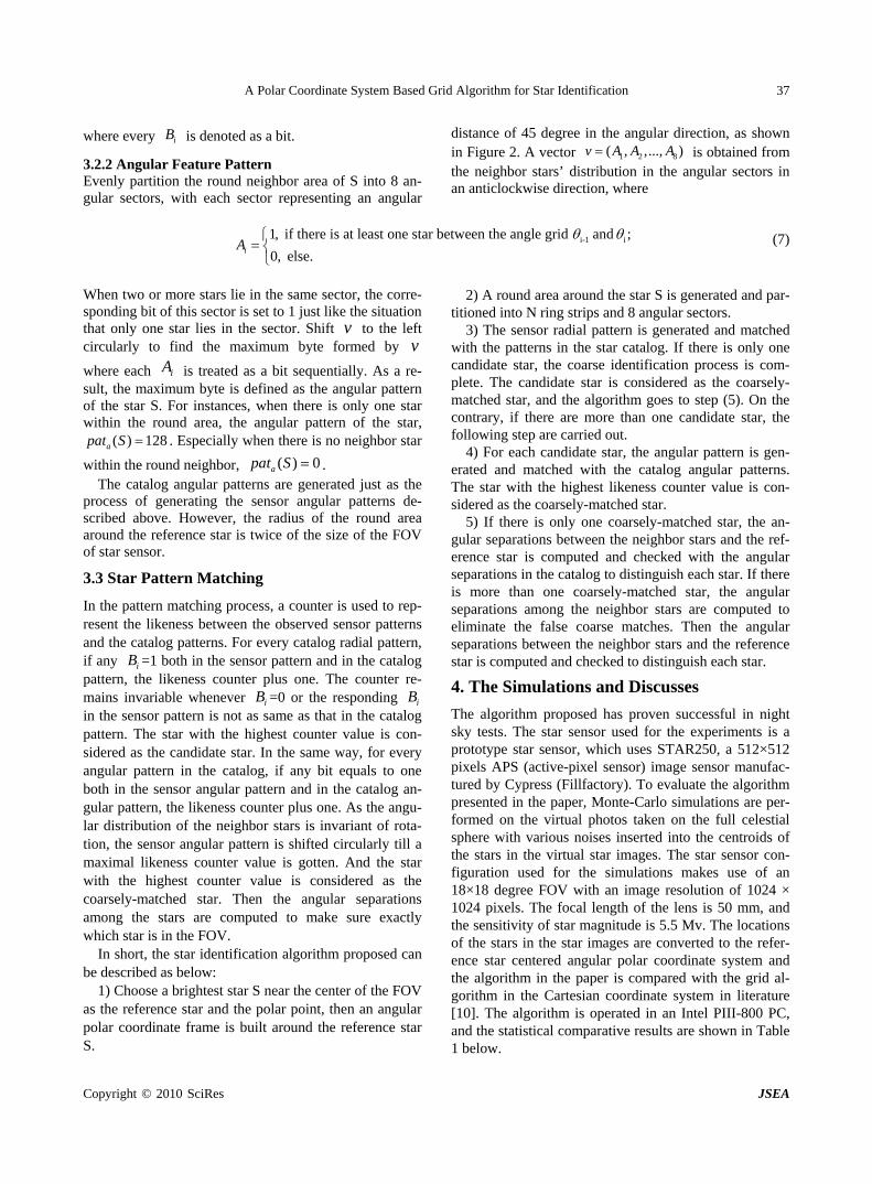
A Polar Coordinate System Based Grid Algorithm for Star Identification 37
where every is denoted as a bit. iB
3.2.2 Angular Feature Pattern Evenly partition the round neighbor area of S into 8 an-gular sectors, with each sector representing an angular
distance of 45 degree in the angular direction, as shown in Figure 2. A vector 1 2 8( , ,..., )v A A A is obtained from the neighbor stars’ distribution in the angular sectors in an anticlockwise direction, where
i-1 i1, if there is at least one star between the angle grid and ;
0, else.iA
(7)
When two or more stars lie in the same sector, the corre-sponding bit of this sector is set to 1 just like the situation that only one star lies in the sector. Shift to the left circularly to find the maximum byte formed by where each
vv
iA is treated as a bit sequentially. As a re-sult, the maximum byte is defined as the angular pattern of the star S. For instances, when there is only one star within the round area, the angular pattern of the star,
. Especially when there is no neighbor star
within the round neighbor, .
( )apat S 128
( ) 0apat S The catalog angular patterns are generated just as the
process of generating the sensor angular patterns de-scribed above. However, the radius of the round area around the reference star is twice of the size of the FOV of star sensor.
3.3 Star Pattern Matching
In the pattern matching process, a counter is used to rep-resent the likeness between the observed sensor patterns and the catalog patterns. For every catalog radial pattern, if any i =1 both in the sensor pattern and in the catalog pattern, the likeness counter plus one. The counter re-mains invariable whenever i
B
B =0 or the responding iB in the sensor pattern is not as same as that in the catalog pattern. The star with the highest counter value is con-sidered as the candidate star. In the same way, for every angular pattern in the catalog, if any bit equals to one both in the sensor angular pattern and in the catalog an-gular pattern, the likeness counter plus one. As the angu-lar distribution of the neighbor stars is invariant of rota-tion, the sensor angular pattern is shifted circularly till a maximal likeness counter value is gotten. And the star with the highest counter value is considered as the coarsely-matched star. Then the angular separations among the stars are computed to make sure exactly which star is in the FOV.
In short, the star identification algorithm proposed can be described as below:
1) Choose a brightest star S near the center of the FOV as the reference star and the polar point, then an angular polar coordinate frame is built around the reference star S.
2) A round area around the star S is generated and par-titioned into N ring strips and 8 angular sectors.
3) The sensor radial pattern is generated and matched with the patterns in the star catalog. If there is only one candidate star, the coarse identification process is com-plete. The candidate star is considered as the coarsely- matched star, and the algorithm goes to step (5). On the contrary, if there are more than one candidate star, the following step are carried out.
4) For each candidate star, the angular pattern is gen-erated and matched with the catalog angular patterns. The star with the highest likeness counter value is con-sidered as the coarsely-matched star.
5) If there is only one coarsely-matched star, the an-gular separations between the neighbor stars and the ref-erence star is computed and checked with the angular separations in the catalog to distinguish each star. If there is more than one coarsely-matched star, the angular separations among the neighbor stars are computed to eliminate the false coarse matches. Then the angular separations between the neighbor stars and the reference star is computed and checked to distinguish each star.
4. The Simulations and Discusses
The algorithm proposed has proven successful in night sky tests. The star sensor used for the experiments is a prototype star sensor, which uses STAR250, a 512×512 pixels APS (active-pixel sensor) image sensor manufac-tured by Cypress (Fillfactory). To evaluate the algorithm presented in the paper, Monte-Carlo simulations are per-formed on the virtual photos taken on the full celestial sphere with various noises inserted into the centroids of the stars in the virtual star images. The star sensor con-figuration used for the simulations makes use of an 18×18 degree FOV with an image resolution of 1024 × 1024 pixels. The focal length of the lens is 50 mm, and the sensitivity of star magnitude is 5.5 Mv. The locations of the stars in the star images are converted to the refer-ence star centered angular polar coordinate system and the algorithm in the paper is compared with the grid al-gorithm in the Cartesian coordinate system in literature [10]. The algorithm is operated in an Intel PIII-800 PC, and the statistical comparative results are shown in Table 1 below.
Copyright © 2010 SciRes JSEA
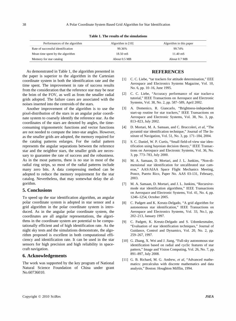
A Polar Coordinate System Based Grid Algorithm for Star Identification 38
Table 1. The results of the simulations
Performances of the algorithm Algorithm in [10] Algorithm in this paper
Rate of successful identification 99.36% 99.74%
Mean time spent by the algorithm 18.50 mS 11.40 mS
Memory for star catalog About 0.5 MB About 0.7 MB
As demonstrated in Table 1, the algorithm presented in
the paper is superior to the algorithm in the Cartesian coordinate system in both the identification rate and the time spent. The improvement in rate of success results from the consideration that the reference star may be near the brim of the FOV, as well as from the smaller radial grids adopted. The failure cases are associated with the noises inserted into the centroids of the stars.
Another improvement of the algorithm is to use the pixel-distribution of the stars in an angular polar coordi-nate system to coarsely identify the reference star. As the coordinates of the stars are denoted by angles, the time- consuming trigonometric functions and vector functions are not needed to compute the inter-star angles. However, as the smaller grids are adopted, the memory required for the catalog patterns enlarges. For the radial pattern represents the angular separations between the reference star and the neighbor stars, the smaller grids are neces-sary to guarantee the rate of success and the robustness. As in the most patterns, there is no star in most of the radial ring strips, so most of the radial patterns include many zero bits. A data compressing method can be adopted to reduce the memory requirement for the star catalog. Nevertheless, that may somewhat delay the al-gorithm.
5. Conclusions
To speed up the star identification algorithm, an angular polar coordinate system is adopted in star sensor and a grid algorithm in the polar coordinate system is intro-duced. As in the angular polar coordinate system, the coordinates are all angular representations, the algori- thms in the coordinate system are potential to be compu-tationally efficient and of high identification rate. As the night sky tests and the simulations demonstrate, the algo-rithm proposed is excellent in both computational effi-ciency and identification rate. It can be used in the star sensors for high precision and high reliability in space-craft navigation.
6. Acknowledgements
The work was supported by the key program of National Natural Science Foundation of China under grant No.60736010.
REFERENCES
[1] C. C. Liebe, “tar trackers for attitude determination,” EEE Aerospace and Electronics Systems Magazine, Vol. 10, No. 6, pp. 10–16, June 1995.
[2] C. C. Liebe, “Accuracy performance of star tracker-a tutorial,” IEEE Transactions on Aerospace and Electronic Systems, Vol. 38, No. 2, pp. 587–589, April 2002.
[3] A. Domenico, R. Giancarlo, “Brightness-independent start-up routine for star trackers,” IEEE Transactions on Aerospace and Electronic Systems, Vol. 38, No. 3, pp. 813–823, July 2002.
[4] D. Mortari, M. A. Samaan, and C. Bruccoleri, et al, “The pyramid star identification technique,” Journal of The In-stitute of Navigation, Vol. 51, No. 3, pp. 171–184, 2004.
[5] S. C. Daniel, W. P. Curtis, “Small field-of-view star iden-tification using bayesian decision theory,” IEEE Transac-tions on Aerospace and Electronic Systems, Vol. 36, No. 3, pp. 773–783, July 2000.
[6] M. A. Samaan, D. Mortari, and J. L. Junkins, “Non-di-mensional star identification for uncalibrated star cam-eras,” AAS/AIAA Space Flight Mechanics Meeting, Ponce, Puerto Rico, Paper No. AAS 03-131, February, 2003.
[7] M. A. Samaan, D. Mortari, and J. L. Junkins, “Recursive- mode star identification algorithms,” IEEE Transactions on Aerospace and Electronic Systems, Vol. 41, No. 4, pp. 1246–1254, October 2005.
[8] C. Padgett and K. Kreutz-Delgado, “A grid algorithm for autonomous star identification,” IEEE Transactions on Aerospace and Electronics Systems, Vol. 33, No.1, pp. 202–213, January 1997.
[9] C. Padgett, K. Kreutz-Delgado and S. Udomkesmalee, “Evaluation of star identification techniques,” Journal of Guidance, Control and Dynamics, Vol. 20, No. 2, pp. 259–267, 1997.
[10] G. Zhang, X. Wei and J. Jiang, “Full-sky autonomous star identification based on radial and cyclic features of star pattern,” Image and Vision Computing, Vol. 26, No. 7, pp. 891–897, July 2008.
[11] G. B. Richard, M. G. Andrew, et al, “Advanced mathe-matics: precalculus with discrete mathematics and data analysis,” Boston: Houghton Mifflin, 1994.
Copyright © 2010 SciRes JSEA

J. Software Engineering & Applications, 2010, 3: 39-49 doi:10.4236/jsea.2010.31005 Published Online January 2010 (http://www.SciRP.org/journal/jsea)
Copyright © 2010 SciRes JSEA
39
Evaluation of Feature Subset Selection, Feature Weighting, and Prototype Selection for Biomedical Applications
Suzanne LITTLE1, Sara COLANTONIO 2, Ovidio SALVETTI2, Petra PERNER1*
1Institute of Computer Vision and Applied Computer Sciences, Germany; 2ISTI-CNR, Pisa, Italy. Email: [email protected] Received September 15th, 2009; revised October 9th, 2009; accepted October 21st, 2009.
ABSTRACT
Many medical diagnosis applications are characterized by datasets that contain under-represented classes due to the fact that the disease is much rarer than the normal case. In such a situation classifiers such as decision trees and Naïve Bayesian that generalize over the data are not the proper choice as classification methods. Case-based classifiers that can work on the samples seen so far are more appropriate for such a task. We propose to calculate the contingency table and class specific evaluation measures despite the overall accuracy for evaluation purposes of classifiers for these specific data characteristics. We evaluate the different options of our case-based classifier and compare the perform-ance to decision trees and Naïve Bayesian. Finally, we give an outlook for further work. Keywords: Feature Subset Selection, Feature Weighting, Prototype Selection, Evaluation of Methods, Prototype-Based
Classification, Methodology for Prototype-Based Classification, CBR in Health
1. Introduction
Many medical diagnosis applications are characterized by datasets that contain under-represented classes due to the fact that the disease is much rarer than the normal case. In such a situation classifiers such as decision trees and Naïve Bayesian that generalize over the data are not the proper choice as classification methods. Decision trees tend to over-generalize the class with the most ex-amples while Naïve Bayesian requires enough data for the estimation of the class-conditional probabilities. Case-based classifiers that can work on the samples seen so far are more appropriate for such a task.
A case-based classifier classifies a new sample by finding similar cases in the case base based on a proper similarity measure. A good coverage of the casebase, the right case description and the proper similarity are the essential functions that enable a case-based classifier to perform well.
In this work we studied the behavior of a case-based classifier based on different medical datasets with dif-ferent characteristics from the UCI repository [1]. We chose datasets where one or more classes were heavily under-represented compared to the other classes as well as datasets having more or less equally distributed sam-ples for the classes for comparison purposes.
The case-based classifier has several options for im-proving its performance that can be chosen independ-ently or in combination. Currently available options in our case-based classifier are: k-value for the closest cases; feature subset selection (FS); feature weight learning (FW); and prototype selection (PS). To con-clusively determine which combination of options is best for the current problem is non-obvious and time- consuming and we hope to develop with our study a methodology that assists a user in designing and refin-ing our case-based classifiers. We observe the influ-ence of the different options of a case-based classifier and report the results in this paper. Our study is an on-going study; we also intend to investigate other op-tions in casebase maintenance.
The aim of this work is to provide the user with a methodology for best applying our case-based classifier and for evaluating the classifier particularly in situations where there is under-representation of specific classes. In Section 2 we describe our case-based classifier named ProtoClass while Section 3 describes the evaluation strategy. The datasets are described in Section 4. Results are reported in Section 5 and a discussion on the results is given in Section 6. Finally, we summarize our work and give an outlook of further work in Section 7.
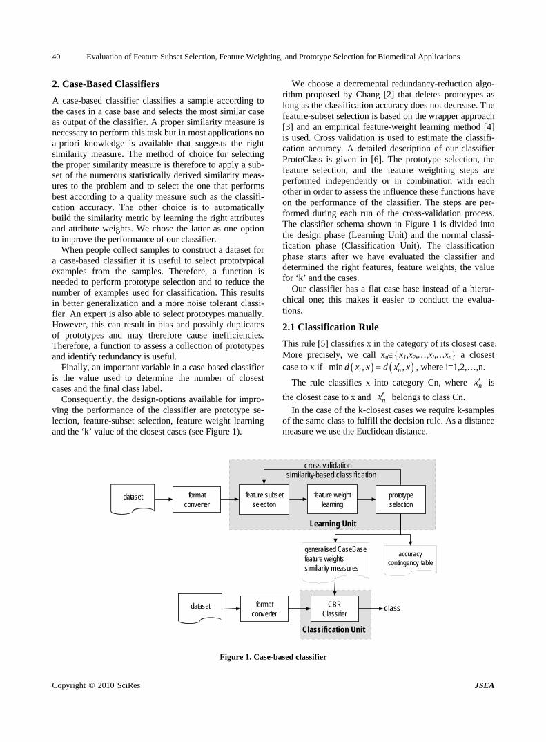
Evaluation of Feature Subset Selection, Feature Weighting, and Prototype Selection for Biomedical Applications 40
2. Case-Based Classifiers
A case-based classifier classifies a sample according to the cases in a case base and selects the most similar case as output of the classifier. A proper similarity measure is necessary to perform this task but in most applications no a-priori knowledge is available that suggests the right similarity measure. The method of choice for selecting the proper similarity measure is therefore to apply a sub-set of the numerous statistically derived similarity meas-ures to the problem and to select the one that performs best according to a quality measure such as the classifi-cation accuracy. The other choice is to automatically build the similarity metric by learning the right attributes and attribute weights. We chose the latter as one option to improve the performance of our classifier.
When people collect samples to construct a dataset for a case-based classifier it is useful to select prototypical examples from the samples. Therefore, a function is needed to perform prototype selection and to reduce the number of examples used for classification. This results in better generalization and a more noise tolerant classi-fier. An expert is also able to select prototypes manually. However, this can result in bias and possibly duplicates of prototypes and may therefore cause inefficiencies. Therefore, a function to assess a collection of prototypes and identify redundancy is useful.
Finally, an important variable in a case-based classifier is the value used to determine the number of closest cases and the final class label.
Consequently, the design-options available for impro- ving the performance of the classifier are prototype se-lection, feature-subset selection, feature weight learning and the ‘k’ value of the closest cases (see Figure 1).
We choose a decremental redundancy-reduction algo-rithm proposed by Chang [2] that deletes prototypes as long as the classification accuracy does not decrease. The feature-subset selection is based on the wrapper approach [3] and an empirical feature-weight learning method [4] is used. Cross validation is used to estimate the classifi-cation accuracy. A detailed description of our classifier ProtoClass is given in [6. The prototype selection, the feature selection, and the feature weighting steps are performed independently or in combination with each other in order to assess the influence these functions have on the performance of the classifier. The steps are per-formed during each run of the cross-validation process. The classifier schema shown in Figure 1 is divided into the design phase (Learning Unit) and the normal classi-fication phase (Classification Unit). The classification phase starts after we have evaluated the classifier and determined the right features, feature weights, the value for ‘k’ and the cases.
Our classifier has a flat case base instead of a hierar-chical one; this makes it easier to conduct the evalua-tions.
2.1 Classification Rule
This rule [5] classifies x in the category of its closest case. More precisely, we call xnx1,x2,…,xi,…xn a closest case to x if min , ,i nd x x d x x , where i=1,2,…,n.
The rule classifies x into category Cn, where nx is
the closest case to x and nx belongs to class Cn.
In the case of the k-closest cases we require k-samples of the same class to fulfill the decision rule. As a distance measure we use the Euclidean distance.
dataset formatconverter
feature subsetselection
feature weightlearning
prototypeselection
generalised CaseBase feature weights similiarity measures
Learning Unit
similarity-based classificationcross validation
CBRClassifier
Classification Unit
classdataset formatconverter
accuracycontingency table
Figure 1. Case-based classifier
Copyright © 2010 SciRes JSEA
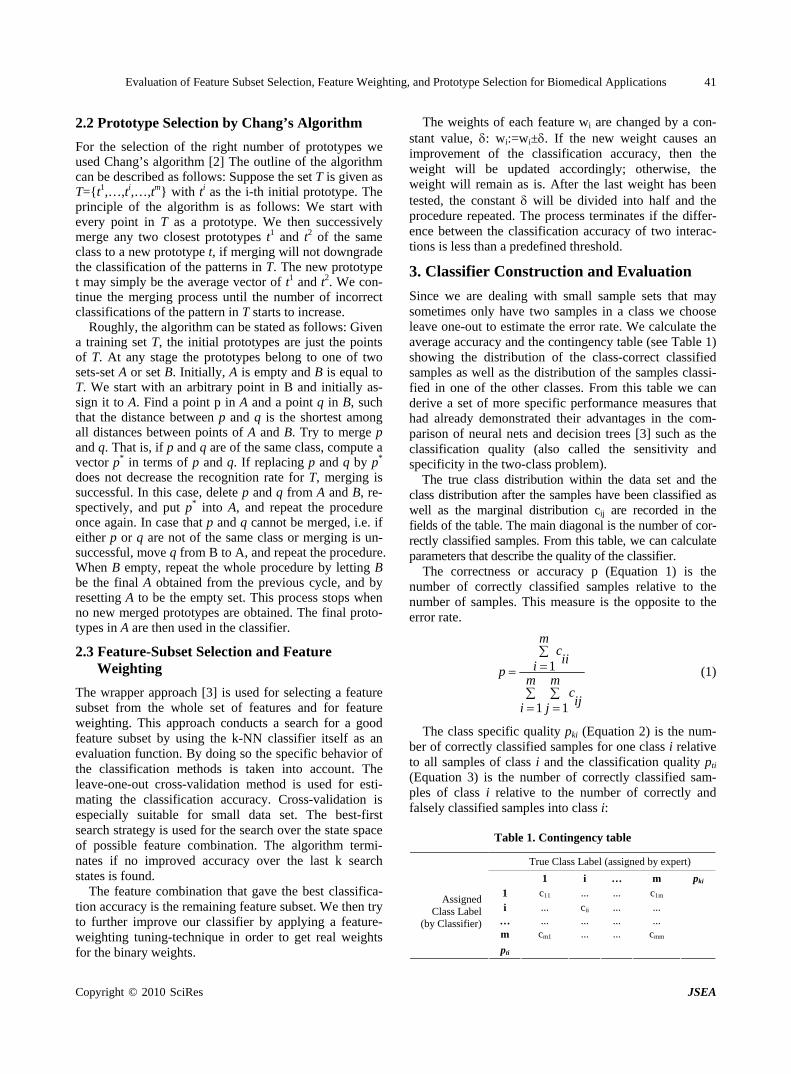
Evaluation of Feature Subset Selection, Feature Weighting, and Prototype Selection for Biomedical Applications 41
2.2 Prototype Selection by Chang’s Algorithm
For the selection of the right number of prototypes we used Chang’s algorithm [2] The outline of the algorithm can be described as follows: Suppose the set T is given as T={t1,…,ti,…,tm} with ti as the i-th initial prototype. The principle of the algorithm is as follows: We start with every point in T as a prototype. We then successively merge any two closest prototypes t1 and t2 of the same class to a new prototype t, if merging will not downgrade the classification of the patterns in T. The new prototype t may simply be the average vector of t1 and t2. We con-tinue the merging process until the number of incorrect classifications of the pattern in T starts to increase.
Roughly, the algorithm can be stated as follows: Given a training set T, the initial prototypes are just the points of T. At any stage the prototypes belong to one of two sets-set A or set B. Initially, A is empty and B is equal to T. We start with an arbitrary point in B and initially as-sign it to A. Find a point p in A and a point q in B, such that the distance between p and q is the shortest among all distances between points of A and B. Try to merge p and q. That is, if p and q are of the same class, compute a vector p* in terms of p and q. If replacing p and q by p* does not decrease the recognition rate for T, merging is successful. In this case, delete p and q from A and B, re-spectively, and put p* into A, and repeat the procedure once again. In case that p and q cannot be merged, i.e. if either p or q are not of the same class or merging is un-successful, move q from B to A, and repeat the procedure. When B empty, repeat the whole procedure by letting B be the final A obtained from the previous cycle, and by resetting A to be the empty set. This process stops when no new merged prototypes are obtained. The final proto-types in A are then used in the classifier.
2.3 Feature-Subset Selection and Feature Weighting
The wrapper approach [3] is used for selecting a feature subset from the whole set of features and for feature weighting. This approach conducts a search for a good feature subset by using the k-NN classifier itself as an evaluation function. By doing so the specific behavior of the classification methods is taken into account. The leave-one-out cross-validation method is used for esti-mating the classification accuracy. Cross-validation is especially suitable for small data set. The best-first search strategy is used for the search over the state space of possible feature combination. The algorithm termi-nates if no improved accuracy over the last k search states is found.
The feature combination that gave the best classifica-tion accuracy is the remaining feature subset. We then try to further improve our classifier by applying a feature- weighting tuning-technique in order to get real weights for the binary weights.
The weights of each feature wi are changed by a con-stant value, : wi:=wi±. If the new weight causes an improvement of the classification accuracy, then the weight will be updated accordingly; otherwise, the weight will remain as is. After the last weight has been tested, the constant will be divided into half and the procedure repeated. The process terminates if the differ-ence between the classification accuracy of two interac-tions is less than a predefined threshold.
3. Classifier Construction and Evaluation
Since we are dealing with small sample sets that may sometimes only have two samples in a class we choose leave one-out to estimate the error rate. We calculate the average accuracy and the contingency table (see Table 1) showing the distribution of the class-correct classified samples as well as the distribution of the samples classi-fied in one of the other classes. From this table we can derive a set of more specific performance measures that had already demonstrated their advantages in the com-parison of neural nets and decision trees [3] such as the classification quality (also called the sensitivity and specificity in the two-class problem).
The true class distribution within the data set and the class distribution after the samples have been classified as well as the marginal distribution cij are recorded in the fields of the table. The main diagonal is the number of cor-rectly classified samples. From this table, we can calculate parameters that describe the quality of the classifier.
The correctness or accuracy p (Equation 1) is the number of correctly classified samples relative to the number of samples. This measure is the opposite to the error rate.
m
i
m
j ijc
m
i iic
p
1 1
1 (1)
The class specific quality pki (Equation 2) is the num-ber of correctly classified samples for one class i relative to all samples of class i and the classification quality pti (Equation 3) is the number of correctly classified sam- ples of class i relative to the number of correctly and falsely classified samples into class i:
Table 1. Contingency table
True Class Label (assigned by expert)
1 i … m pki 1 c11 ... ... c1m i ... cii ... ...
… ... ... ... ... m cm1 ... ... cmm
Assigned Class Label
(by Classifier)
pti
Copyright © 2010 SciRes JSEA
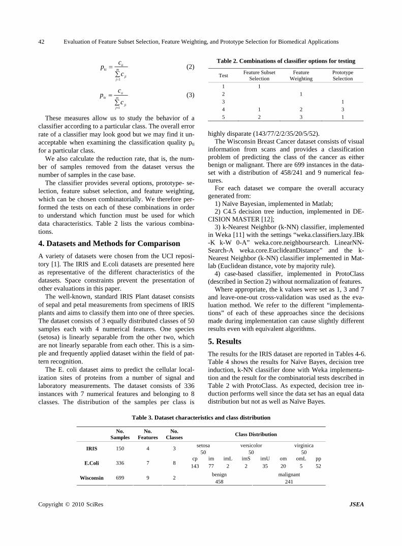
Evaluation of Feature Subset Selection, Feature Weighting, and Prototype Selection for Biomedical Applications 42
m
jji
iiki
c
cp
1
(2)
m
jji
iiki
c
cp
1
(3)
These measures allow us to study the behavior of a classifier according to a particular class. The overall error rate of a classifier may look good but we may find it un-acceptable when examining the classification quality pti for a particular class.
We also calculate the reduction rate, that is, the num-ber of samples removed from the dataset versus the number of samples in the case base.
The classifier provides several options, prototype- se-lection, feature subset selection, and feature weighting, which can be chosen combinatorially. We therefore per-formed the tests on each of these combinations in order to understand which function must be used for which data characteristics. Table 2 lists the various combina-tions.
4. Datasets and Methods for Comparison
A variety of datasets were chosen from the UCI reposi-tory [1]. The IRIS and E.coli datasets are presented here as representative of the different characteristics of the datasets. Space constraints prevent the presentation of other evaluations in this paper.
The well-known, standard IRIS Plant dataset consists of sepal and petal measurements from specimens of IRIS plants and aims to classify them into one of three species. The dataset consists of 3 equally distributed classes of 50 samples each with 4 numerical features. One species (setosa) is linearly separable from the other two, which are not linearly separable from each other. This is a sim-ple and frequently applied dataset within the field of pat-tern recognition.
The E. coli dataset aims to predict the cellular local-ization sites of proteins from a number of signal and laboratory measurements. The dataset consists of 336 instances with 7 numerical features and belonging to 8 classes. The distribution of the samples per class is
Table 2. Combinations of classifier options for testing
Test Feature Subset
Selection Feature
Weighting Prototype Selection
1 1
2 1
3 1
4 1 2 3
5 2 3 1
highly disparate (143/77/2/2/35/20/5/52).
The Wisconsin Breast Cancer dataset consists of visual information from scans and provides a classification problem of predicting the class of the cancer as either benign or malignant. There are 699 instances in the data-set with a distribution of 458/241 and 9 numerical fea-tures.
For each dataset we compare the overall accuracy generated from:
1) Naïve Bayesian, implemented in Matlab; 2) C4.5 decision tree induction, implemented in DE-
CISION MASTER [12]; 3) k-Nearest Neighbor (k-NN) classifier, implemented
in Weka [11] with the settings “weka.classifiers.lazy.IBk -K k-W 0-A” weka.core.neighboursearch. LinearNN-Search-A weka.core.EuclideanDistance” and the k- Nearest Neighbor (k-NN) classifier implemented in Mat-lab (Euclidean distance, vote by majority rule).
4) case-based classifier, implemented in ProtoClass (described in Section 2) without normalization of features.
Where appropriate, the k values were set as 1, 3 and 7 and leave-one-out cross-validation was used as the eva- luation method. We refer to the different “implementa-tions” of each of these approaches since the decisions made during implementation can cause slightly different results even with equivalent algorithms.
5. Results
The results for the IRIS dataset are reported in Tables 4-6. Table 4 shows the results for Naïve Bayes, decision tree induction, k-NN classifier done with Weka implementa-tion and the result for the combinatorial tests described in Table 2 with ProtoClass. As expected, decision tree in-duction performs well since the data set has an equal data distribution but not as well as Naïve Bayes.
Table 3. Dataset characteristics and class distribution
No.
Samples No.
Features No.
ClassesClass Distribution
setosa versicolor virginica IRIS 150 4 3
50 50 50 cp im imL imS imU om omL pp
E.Coli 336 7 8 143 77 2 2 35 20 5 52
benign malignant Wisconsin 699 9 2
458 241
Copyright © 2010 SciRes JSEA

Evaluation of Feature Subset Selection, Feature Weighting, and Prototype Selection for Biomedical Applications 43
Table 4. Overall accuracy for IRIS dataset using leave-one-out
k Naïve Bayes
Deci-sion Tree
kNN Proto-Class
Feature Subset
Feature Weighting
Prototype Selection
FS+ FW+ PS
PS+ FS+ FW
1 95.33 96.33 95.33 96.00 X X 96.00 96.00 96.33 3 na na 95.33 96.00 96.33 96.33 96.00 96.33 96.00 7 na na 96.33 96.67 X 96.00 96.00 96.33 96.00
Table 5. Contingency table for k=1,3,7 for the IRIS dataset and protoclass
IRIS setosa versicolor Virginica
k 1 3 7 1 3 7 1 3 7
setosa 50 50 50 0 0 0 0 0 0
versicolor 0 0 0 47 47 46 3 3 4
virginica 0 0 0 3 3 1 47 47 49
Classification quality 100 100 100 94 94 97.87 94 94 92.45
Class specific quality 100 100 100 94 94 92 94 94 98
Table 6. Class distribution and percentage reduction rate of IRIS dataset after prototype selection
Iris-
sertosa Iris-
versicolor Iris-
virginica Reduction Rate in %
orig 50 50 50 0.00
k=1 50 49 50 0.67
k=3 50 49 50 0.67
k=7 50 48 50 1.33
In general we can say that the accuracy does not sig-nificantly improve when using feature subset selection, feature weighting and prototype selection with Proto-Class. In case of k=1 and k=7 the feature subset remains the initial feature set. This is marked in Table 4 by an “X” indicating that no changes were made in the design phase and the accuracy is the same as for the initial clas-sifier. This is not surprising since the data base contains
Table 7. Overall accuracy for E. coli dataset using leave-one-out
k Naïve Bayes
Decision Tree
Weka Near-est
Neighbour
Matlab knn
ProtoClass Feature Subset
(FS)
Feature Weighting
(FW)
Prototype Selection
(PS)
FS+FW+ PS
PS+FS+ FW
1 86.01 66.37 80.95 80.06 81.25 80.95 83.04 80.65 82.44 80.95 3 na na 83.93 84.26 84.23 85.12 84.23 82.74 83.93 82.74 7 na na 86.40 86.31 87.20 87.20 86.31 86.61 85.42 86.61
Table 8. Combined contingency table for k=1,3,7 for the E. coli dataset and protoClass
cp im imL imS imU Om omL pp
k 1 3 7 1 3 7 1 3 7 1 3 7 1 3 7 1 3 7 1 3 7 1 3 7
cp 133 139 140 4 0 0 0 0 0 0 0 0 0 0 0 0 0 0 0 0 0 6 4 3
im 3 4 3 56 60 60 1 0 0 1 0 0 15 12 11 0 0 0 0 0 0 1 0 3
imL 0 0 0 1 1 1 0 0 0 0 0 0 0 0 0 0 0 0 1 1 1 0 0 0
imS 0 0 0 0 0 0 0 0 0 0 0 0 1 1 1 0 0 0 0 0 0 1 1 1
imU 1 1 1 15 16 12 0 0 0 0 0 0 19 17 22 0 1 0 0 0 0 0 0 0
om 0 0 0 0 0 0 0 0 0 0 0 0 1 0 0 16 17 17 0 1 1 3 2 2
omL 0 0 0 0 0 0 0 0 0 0 0 0 0 0 0 0 0 0 5 5 5 0 0 0
pp 5 4 4 1 1 1 0 0 0 0 0 0 0 0 0 2 2 0 0 0 0 44 45 47
pki 93.66 93.92 94.59 72.73 76.92 81.08 0.00 0 0 0.00 0 0 52.78 56.67 64.71 88.89 85.00 100.00 83.33 71.43 71.43 80.00 86.54 83.93
pti 93.01 97.20 97.90 72.73 78.95 77.92 0.00 0.00 0.00 0.00 0.00 0.00 54.29 48.57 62.86 80.00 85.00 85.00 100.00 100.00 100.00 84.62 86.54 90.38
only 4 features which are more or less well-distinguished. In case of k=3 a decrease in accuracy is observed al-though the stopping criteria for the methods for feature subset selection and feature weighting require the overall
accuracy not to decrease. This accuracy is calculated within the loop of the cross validation cycle on the de-sign data set and afterwards the single left out sample is classified against the new learnt classifier to calculate the
Copyright © 2010 SciRes JSEA
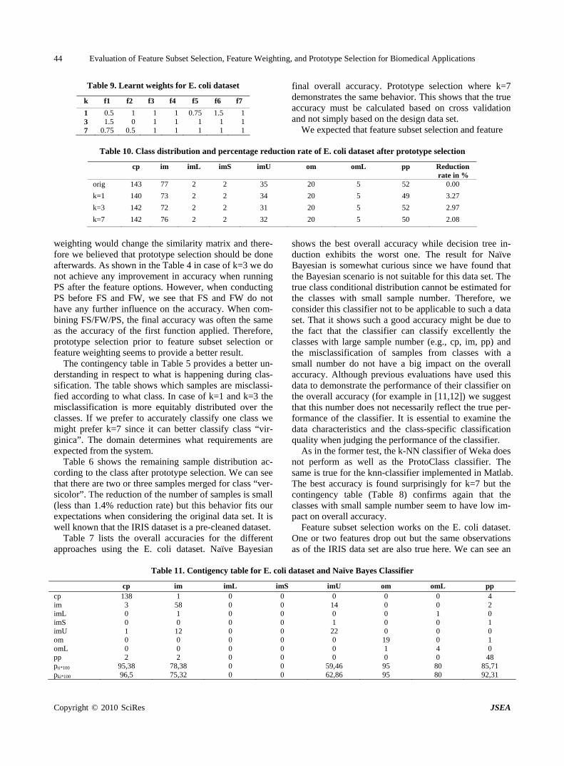
Evaluation of Feature Subset Selection, Feature Weighting, and Prototype Selection for Biomedical Applications 44
Table 9. Learnt weights for E. coli dataset
k f1 f2 f3 f4 f5 f6 f7
1 0.5 1 1 1 0.75 1.5 13 1.5 0 1 1 1 1 17 0.75 0.5 1 1 1 1 1
final overall accuracy. Prototype selection where k=7 demonstrates the same behavior. This shows that the true accuracy must be calculated based on cross validation and not simply based on the design data set.
We expected that feature subset selection and feature
Table 10. Class distribution and percentage reduction rate of E. coli dataset after prototype selection
cp im imL imS imU om omL pp Reduction rate in %
orig 143 77 2 2 35 20 5 52 0.00
k=1 140 73 2 2 34 20 5 49 3.27
k=3 142 72 2 2 31 20 5 52 2.97
k=7 142 76 2 2 32 20 5 50 2.08
weighting would change the similarity matrix and there-fore we believed that prototype selection should be done afterwards. As shown in the Table 4 in case of k=3 we do not achieve any improvement in accuracy when running PS after the feature options. However, when conducting PS before FS and FW, we see that FS and FW do not have any further influence on the accuracy. When com-bining FS/FW/PS, the final accuracy was often the same as the accuracy of the first function applied. Therefore, prototype selection prior to feature subset selection or feature weighting seems to provide a better result.
The contingency table in Table 5 provides a better un-derstanding in respect to what is happening during clas-sification. The table shows which samples are misclassi-fied according to what class. In case of k=1 and k=3 the misclassification is more equitably distributed over the classes. If we prefer to accurately classify one class we might prefer k=7 since it can better classify class “vir-ginica”. The domain determines what requirements are expected from the system.
Table 6 shows the remaining sample distribution ac-cording to the class after prototype selection. We can see that there are two or three samples merged for class “ver-sicolor”. The reduction of the number of samples is small (less than 1.4% reduction rate) but this behavior fits our expectations when considering the original data set. It is well known that the IRIS dataset is a pre-cleaned dataset.
Table 7 lists the overall accuracies for the different approaches using the E. coli dataset. Naïve Bayesian
shows the best overall accuracy while decision tree in-duction exhibits the worst one. The result for Naïve Bayesian is somewhat curious since we have found that the Bayesian scenario is not suitable for this data set. The true class conditional distribution cannot be estimated for the classes with small sample number. Therefore, we consider this classifier not to be applicable to such a data set. That it shows such a good accuracy might be due to the fact that the classifier can classify excellently the classes with large sample number (e.g., cp, im, pp) and the misclassification of samples from classes with a small number do not have a big impact on the overall accuracy. Although previous evaluations have used this data to demonstrate the performance of their classifier on the overall accuracy (for example in [11,12]) we suggest that this number does not necessarily reflect the true per-formance of the classifier. It is essential to examine the data characteristics and the class-specific classification quality when judging the performance of the classifier.
As in the former test, the k-NN classifier of Weka does not perform as well as the ProtoClass classifier. The same is true for the knn-classifier implemented in Matlab. The best accuracy is found surprisingly for k=7 but the contingency table (Table 8) confirms again that the classes with small sample number seem to have low im-pact on overall accuracy.
Feature subset selection works on the E. coli dataset. One or two features drop out but the same observations as of the IRIS data set are also true here. We can see an
Table 11. Contigency table for E. coli dataset and Naïve Bayes Classifier
cp im imL imS imU om omL pp cp 138 1 0 0 0 0 0 4 im 3 58 0 0 14 0 0 2 imL 0 1 0 0 0 0 1 0 imS 0 0 0 0 1 0 0 1 imU 1 12 0 0 22 0 0 0 om 0 0 0 0 0 19 0 1 omL 0 0 0 0 0 1 4 0 pp 2 2 0 0 0 0 0 48 pti*100 95,38 78,38 0 0 59,46 95 80 85,71 pki*100 96,5 75,32 0 0 62,86 95 80 92,31
Copyright © 2010 SciRes JSEA
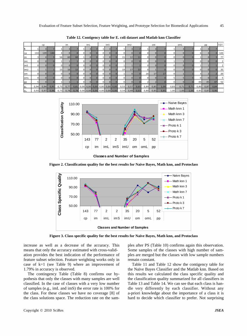
Evaluation of Feature Subset Selection, Feature Weighting, and Prototype Selection for Biomedical Applications 45
Table 12. Contigency table for E. coli dataset and Matlab knn Classifier
TOT
k 1 3 7 1 3 7 1 3 7 1 3 7 1 3 7 1 3 7 1 3 7 1 3 7
cp 133 139 140 4 0 0 0 0 0 0 0 0 0 0 0 0 0 0 0 0 0 6 4 3 14
im 3 4 3 56 60 60 1 0 0 1 0 0 15 12 11 0 0 0 0 0 0 1 0 3 7
imL 0 0 0 1 1 1 0 0 0 0 0 0 0 0 0 0 0 0 1 1 1 0 0 0
imS 0 0 0 0 0 0 0 0 0 0 0 0 1 1 1 0 0 0 0 0 0 1 1 1
imU 1 1 1 15 16 12 0 0 0 0 0 0 19 17 22 0 1 0 0 0 0 0 0 0 3
om 0 0 0 0 0 0 0 0 0 0 0 0 1 0 0 16 17 17 0 1 1 3 2 2 2
omL 0 0 0 0 0 0 0 0 0 0 0 0 0 0 0 0 0 0 5 5 5 0 0 0
pp 5 4 4 1 1 1 0 0 0 0 0 0 0 0 0 2 2 0 0 0 0 44 45 47 5
pti 0,94 0,94 0,95 0,73 0,77 0,81 0,00 0,00 0,00 0,00 0,00 0,00 0,53 0,57 0,65 0,89 0,85 1,00 0,83 0,71 0,71 0,80 0,87 0,84
pki 0,93 0,97 0,98 0,73 0,78 0,78 0,00 0,00 0,00 0,00 0,00 0,00 0,54 0,49 0,63 0,80 0,85 0,85 1,00 1,00 1,00 0,85 0,87 0,90
omL ppcp im imL imS imU om
3
7
2
2
5
0
5
2
50.00
70.00
90.00
110.00
143 77 2 2 35 20 5 52
cp im imL imS imU om omL pp
Classes and Number of Samples
Cla
ssif
icat
ion
Qu
alit
y Naive Bayes
Math knn 1
Math knn 3
Math knn 7
Proto k 1
Proto k 3
Proto k 7
Figure 2. Classification quality for the best results for Naïve Bayes, Math knn, and Protoclass
50.00
70.00
90.00
110.00
143 77 2 2 35 20 5 52
cp im imL imS imU om omL pp
Classes and Number of Samples
Cla
ss S
pec
ific
Qu
alit
y Naive Bayes
Math knn 1
Math knn 3
Math knn 7
Proto k 1
Proto k 3
Proto k 7
Figure 3. Class specific quality for the best results for Naïve Bayes, Math knn, and Protoclass
increase as well as a decrease of the accuracy. This means that only the accuracy estimated with cross-valid- ation provides the best indication of the performance of feature subset selection. Feature weighting works only in case of k=1 (see Table 9) where an improvement of 1.79% in accuracy is observed.
The contingency Table (Table 8) confirms our hy-pothesis that only the classes with many samples are well classified. In the case of classes with a very low number of samples (e.g., imL and imS) the error rate is 100% for the class. For these classes we have no coverage [8] of the class solutions space. The reduction rate on the sam-
ples after PS (Table 10) confirms again this observation. Some samples of the classes with high number of sam-ples are merged but the classes with low sample numbers remain constant.
Table 11 and Table 12 show the contigency table for the Naïve Bayes Classifier and the Matlab knn. Based on this results we calculated the class specific quality and the classification quality summarized for all classifiers in Table 13 and Table 14. We can see that each class is han-dle very differently by each classifier. Without any a-priori knowledge about the importance of a class it is hard to decide which classifier to prefer. Not surprising
Copyright © 2010 SciRes JSEA
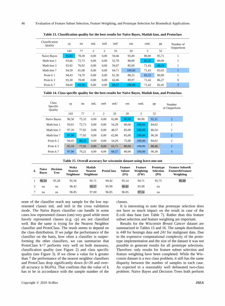
Evaluation of Feature Subset Selection, Feature Weighting, and Prototype Selection for Biomedical Applications 46
Table 13. Classification quality for the best results for Naïve Bayes, Matlab knn, and Protoclass
Table 14. Class specific quality for the best results for Naïve Bayes, Matlab knn, and Protoclass
cp im imL imS imU om omL pp Class Specific Quality
143 77 2 2 35 20 5 52
Number of Outperform
Naive Bayes 96,50 75,32 0,00 0,00 62,86 95,00 80,00 92,31 2
Math knn 1 93,01 72,73 0,00 0,00 54,29 80,00 100,00 84,62 1
Math knn 3 97,20 77,92 0,00 0,00 48,57 85,00 100,00 86,54 1
Math knn 7 97,90 77,92 0,00 0,00 62,86 85,00 100,00 90,38 2
Proto k 1 94,41 80,52 0,00 0,00 54,29 75,00 100,00 84,62 2
Proto k 3 95,10 77,92 0,00 0,00 65,71 80,00 100,00 88,46 1
Proto k 7 97,90 79,22 0,00 0,00 68,57 80,00 100,00 90,38 3
Table 15. Overall accuracy for wisconsin dataset using leave-one-out
k Naïve Bayes
Decision Tree
Weka Nearest
Neighbour
Matlab Nearest
NeighbourProtoClass
Feature Subset
(FS)
Feature Weighting
(FW)
Prototype Selection
(PS)
Feature Subset& Feature&Feature
Weighting
1 96.14 95.28 95.56 95.71 94.42 95.14 94.71 95,75 96.48
3 na na 96.42 96.57 95.99 96.42 95.99 na
7 na na 96.85 97.00 96.85 96.85 97.14 na
none of the classifier reach any sample for the low rep-resented classes imL and imS in the cross validation mode. The Naïve Bayes classifier can handle in some cases low represented classes (om) very good while more havely represented classes (e.g. cp) are not classified well. But the same is trying for the Nearest Neighbor classifier and ProtoClass. The result seems to depend on the class distribution. If we judge the performance of the classifier on the basis, how often a classifier is outper-forming the other classifiers, we can summarize that ProtoClass k=7 performs very well on both measures, classification quality (see Figure 2) and class specific quality (see Figure 3). If we chose a value for k greater than 7 the performance of the nearest neighbor classifiers and ProtoClass drop significantly down (k=20 and over-all accuracy is 84,6%). That confirms that the value of k has to be in accordance with the sample number of the
classes. It is interesting to note that prototype selection does
not have so much impact on the result in case of the E.coli data base (see Table 7). Rather than this feature subset selection and feature weighting are important.
Results for the Wisconsin Breast Cancer dataset are summarized in Tables 15 and 16. The sample distribution is 448 for beningn data and 241 for malignant data. Due to the expensive computational complexity of the proto-type implementation and the size of the dataset it was not possible to generate results for all prototype selections. Therefore: only results for feature subset selection and feature weighting have been completed. While the Wis-consin dataset is a two class problem, it still has the same disparity between the number of samples in each case. As expected in a reasonably well delineated two-class problem: Naïve Bayes and Decision Trees both perform
Classification Quality
cp im imL imS imU om omL pp
143 77 2 2 35 20 5 52
Number of Outperform
Naive Bayes 95,83 78,38 0,00 0,00 59,46 95,00 80,00 85,71 1
Math knn 1 93,66 72,73 0,00 0,00 52,78 88,89 83,33 80,00 1
Math knn 3 93,92 76,92 0,00 0,00 56,67 85,00 71,43 86,54 1
Math knn 7 94,59 81,08 0,00 0,00 64,71 100,00 71,43 83,93 1
Proto k 1 94,43 74,70 0,00 0,00 61,30 88,23 83,33 80,00 1
Proto k 3 93,30 78,00 0,00 0,00 62,06 89,97 71,42 86,27 0
Proto k 7 94,60 83,56 0,00 0,00 68,57 100,00 71,42 82,45 3
Copyright © 2010 SciRes JSEA
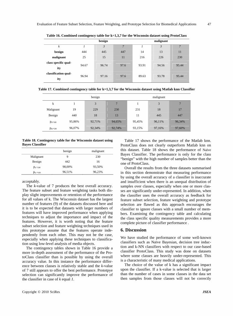
Evaluation of Feature Subset Selection, Feature Weighting, and Prototype Selection for Biomedical Applications 47
Table 16. Combined contingency table for k=1,3,7 for the Wisconsin dataset using ProtoClass
benign malignant
k 1 3 7 1 3 7
benign 444 445 447 14 13 11
malignant 25 15 11 216 226 230
class specific qual-
ity 94.67 96.74 97.6 93.91 94.56 95.44
classification qual-
ity 96.94 97.16 97.6 89.63 93.78 95.44
Table 17. Combined contingency table for k=1,3,7 for the Wisconsin dataset using Matlab knn Classifier
benign malignant
k 1 3 7 1 3 7
Malignant 19 229 230 231 18 17
Benign 440 18 13 11 445 447
pti*100 95,86% 92,71% 94,65% 95,45% 96,11% 96,34%
pki*100 96,07% 92,34% 92,74% 93,15% 97,16% 97,60%
Table 18. Contingency table for the Wisconsin dataset using Bayes Classifier
benign malignant
Malignant 9 230
Benign 442 16
pti *100 98,00% 93,50%
pki *100 96,51% 96,23%
acceptably.
The k-value of 7 produces the best overall accuracy. The feature subset and feature weighting tasks both dis-play slight improvements or retention of the performance for all values of k. The Wisconsin dataset has the largest number of features (9) of the datasets discussed here and it is to be expected that datasets with larger numbers of features will have improved performance when applying techniques to adjust the importance and impact of the features. However, it is worth noting that the feature subset selection and feature weighting techniques used in this prototype assume that the features operate inde-pendently from each other. This may not be the case, especially when applying these techniques to classifica-tion using low-level analysis of media objects.
The contingency tables shown in Table 16 provide a more in-depth assessment of the performance of the Pro-toClass classifier than is possible by using the overall accuracy value. In this instance the performance differ-ence between classes is relatively stable and the k-value of 7 still appears to offer the best performance. Prototpye selection can significantly improve the performance of the classifier in case of k equal 1.
Table 17 shows the performance of the Matlab knn. ProtoClass does not clearly outperform Matlab knn on this dataset. Table 18 shows the performance of Naïve Bayes Classifier. The performance is only for the class “benign” with the high number of samples better than the one of ProtoClass.
Overall the results from the three datasets summarised in this section demonstrate that measuring performance by using the overall accuracy of a classifier is inaccurate and insufficient when there is an unequal distribution of samples over classes, especially when one or more clas- ses are significantly under-represented. In addition, when the classifier uses the overall accuracy as feedback for feature subset selection, feature weighting and prototype selection are flawed as this approach encourages the classifier to ignore classes with a small number of mem-bers. Examining the contingency table and calculating the class specific quality measurements provides a more complete picture of classifier performance .
6. Discussion
We have studied the performance of some well-known classifiers such as Naïve Bayesian, decision tree induc-tion and k-NN classifiers with respect to our case-based classifier ProtoClass. This study was done on datasets where some classes are heavily under-represented. This is a characteristic of many medical applications.
The choice of the value of k has a significant impact upon the classifier. If a k-value is selected that is larger than the number of cases in some classes in the data set then samples from those classes will not be correctly
Copyright © 2010 SciRes JSEA
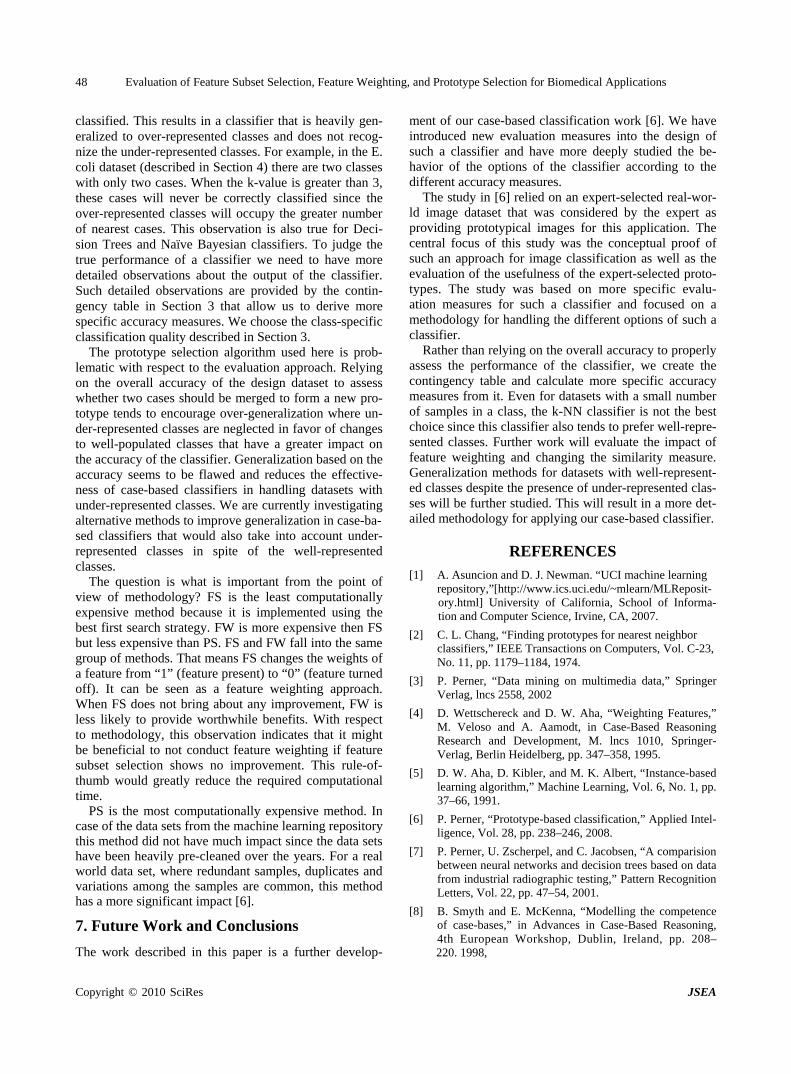
Evaluation of Feature Subset Selection, Feature Weighting, and Prototype Selection for Biomedical Applications 48
classified. This results in a classifier that is heavily gen-eralized to over-represented classes and does not recog-nize the under-represented classes. For example, in the E. coli dataset (described in Section 4) there are two classes with only two cases. When the k-value is greater than 3, these cases will never be correctly classified since the over-represented classes will occupy the greater number of nearest cases. This observation is also true for Deci-sion Trees and Naïve Bayesian classifiers. To judge the true performance of a classifier we need to have more detailed observations about the output of the classifier. Such detailed observations are provided by the contin-gency table in Section 3 that allow us to derive more specific accuracy measures. We choose the class-specific classification quality described in Section 3.
The prototype selection algorithm used here is prob-lematic with respect to the evaluation approach. Relying on the overall accuracy of the design dataset to assess whether two cases should be merged to form a new pro-totype tends to encourage over-generalization where un-der-represented classes are neglected in favor of changes to well-populated classes that have a greater impact on the accuracy of the classifier. Generalization based on the accuracy seems to be flawed and reduces the effective-ness of case-based classifiers in handling datasets with under-represented classes. We are currently investigating alternative methods to improve generalization in case-ba- sed classifiers that would also take into account under- represented classes in spite of the well-represented classes.
The question is what is important from the point of view of methodology? FS is the least computationally expensive method because it is implemented using the best first search strategy. FW is more expensive then FS but less expensive than PS. FS and FW fall into the same group of methods. That means FS changes the weights of a feature from “1” (feature present) to “0” (feature turned off). It can be seen as a feature weighting approach. When FS does not bring about any improvement, FW is less likely to provide worthwhile benefits. With respect to methodology, this observation indicates that it might be beneficial to not conduct feature weighting if feature subset selection shows no improvement. This rule-of- thumb would greatly reduce the required computational time.
PS is the most computationally expensive method. In case of the data sets from the machine learning repository this method did not have much impact since the data sets have been heavily pre-cleaned over the years. For a real world data set, where redundant samples, duplicates and variations among the samples are common, this method has a more significant impact [6].
7. Future Work and Conclusions
The work described in this paper is a further develop-
ment of our case-based classification work [6]. We have introduced new evaluation measures into the design of such a classifier and have more deeply studied the be-havior of the options of the classifier according to the different accuracy measures.
The study in [6] relied on an expert-selected real-wor- ld image dataset that was considered by the expert as providing prototypical images for this application. The central focus of this study was the conceptual proof of such an approach for image classification as well as the evaluation of the usefulness of the expert-selected proto-types. The study was based on more specific evalu- ation measures for such a classifier and focused on a methodology for handling the different options of such a classifier.
Rather than relying on the overall accuracy to properly assess the performance of the classifier, we create the contingency table and calculate more specific accuracy measures from it. Even for datasets with a small number of samples in a class, the k-NN classifier is not the best choice since this classifier also tends to prefer well-repre- sented classes. Further work will evaluate the impact of feature weighting and changing the similarity measure. Generalization methods for datasets with well-represent- ed classes despite the presence of under-represented clas- ses will be further studied. This will result in a more det- ailed methodology for applying our case-based classifier.
REFERENCES
[1] A. Asuncion and D. J. Newman. “UCI machine learning repository,”[http://www.ics.uci.edu/~mlearn/MLReposit- ory.html] University of California, School of Informa- tion and Computer Science, Irvine, CA, 2007.
[2] C. L. Chang, “Finding prototypes for nearest neighbor classifiers,” IEEE Transactions on Computers, Vol. C-23, No. 11, pp. 1179–1184, 1974.
[3] P. Perner, “Data mining on multimedia data,” Springer Verlag, lncs 2558, 2002
[4] D. Wettschereck and D. W. Aha, “Weighting Features,” M. Veloso and A. Aamodt, in Case-Based Reasoning Research and Development, M. lncs 1010, Springer- Verlag, Berlin Heidelberg, pp. 347–358, 1995.
[5] D. W. Aha, D. Kibler, and M. K. Albert, “Instance-based learning algorithm,” Machine Learning, Vol. 6, No. 1, pp. 37–66, 1991.
[6] P. Perner, “Prototype-based classification,” Applied Intel-ligence, Vol. 28, pp. 238–246, 2008.
[7] P. Perner, U. Zscherpel, and C. Jacobsen, “A comparision between neural networks and decision trees based on data from industrial radiographic testing,” Pattern Recognition Letters, Vol. 22, pp. 47–54, 2001.
[8] B. Smyth and E. McKenna, “Modelling the competence of case-bases,” in Advances in Case-Based Reasoning, 4th European Workshop, Dublin, Ireland, pp. 208– 220. 1998,
Copyright © 2010 SciRes JSEA

Evaluation of Feature Subset Selection, Feature Weighting, and Prototype Selection for Biomedical Applications
Copyright © 2010 SciRes JSEA
49
[9] I. H. Witten and E. Frank, Data Mining: Practical ma-chine learning tools and techniques, 2nd Edition, Morgan Kaufmann, San Francisco, 2005.
[10] DECISION MASTER, http://www.ibai-solutions.de.
[11] P. Horton and K. Nakai, “Better prediction of protein cel-lular localization sites with the it k nearest neighbors clas-sifier” Proceeding of the International Conference on Intel-
ligent Systems in Molecular Biology, pp. 147–152 1997.
[12] C. A. Ratanamahatana and D. Gunopulos. “Scaling up the Naive Bayesian Classifier: Using decision trees for fea-ture selection,” in proceedings of Workshop on Data Cleaning and Preprocessing (DCAP 2002), at IEEE In-ternational Conference on Data Mining (ICDM 2002), Maebashi, Japan. 2002.
J. Software Engineering & Applications, 2010, 3: 50-57 doi:10.4236/jsea.2010.31006 Published Online January 2010 (http://www.SciRP.org/journal/jsea)
Copyright © 2010 SciRes JSEA
Cryptanalysis of TEA Using Quantum-Inspired Genetic Algorithms
Wei Hu
Department of Computer Science, Houghton College, One Willard Avenue, Houghton, NY, USA. Email: [email protected] Received September 10th, 2009; revised October 9th, 2009; accepted October 16th, 2009.
ABSTRACT
The Tiny Encryption Algorithm (TEA) is a Feistel block cipher well known for its simple implementation, small memory footprint, and fast execution speed. In two previous studies, genetic algorithms (GAs) were employed to investigate the randomness of TEA output, based on which distinguishers for TEA could be designed. In this study, we used quan-tum-inspired genetic algorithms (QGAs) in the cryptanalysis of TEA. Quantum chromosomes in QGAs have the advan-tage of containing more information than the binary counterpart of the same length in GAs, and therefore generate a more diverse solution pool. We showed that QGAs could discover distinguishers for reduced cycle TEA that are more efficient than those found by classical GAs in two earlier studies. Furthermore, we applied QGAs to break four-cycle and five-cycle TEAs, a considerably harder problem, which the prior GA approach failed to solve. Keywords: Cryptanalysis, Distinguisher, Feistel Block Cipher, Genetic Algorithms, Optimization, Quantum Computing, TEA
1. Introduction
The Tiny Encryption Algorithm (TEA), a Feistel block cipher notable for its simplicity of description and im-plementation, was developed by David Wheeler and Roger Needham at the Computer Laboratory of Cam-bridge University and was first presented at the Fast Software Encryption workshop at Cambridge in 1994 [1]. Its design goal was to minimize the memory footprint and maximize the speed. There is an excellent article on TEA by Shepherd [2].
The following code presents the TEA encode routine in C language:
void code(long* v, long* k) { unsigned long y = v[0], z = v[1], sum = 0, /* set up */ delta = 0x9e3779b9, n = 32 ; while (n-->0) { /* basic cycle start */ sum += delta ; y += (z<<4)+k[0] ^ z+sum ^ (z>>5)+k[1] ; z += (y<<4)+k[2] ^ y+sum ^ (y>>5)+k[3] ; } v[0] = y ; v[1] = z ; }
where the 128-bit key is stored in four 32-bit blocks k = (k[0], k[1], k[2], k[3]) and data of 64 bits are stored in v = (v[0] ,v[1]).
The quantity delta in the C code is used to ensure that encryption/decryption in each cycle is different. A cycle
in TEA is defined as two Feistel rounds. The SHIFT, ADD, and XOR operations in TEA provide the necessary diffusion of the statistics of the plaintext in the ciphertext and confusion between the ciphertext and key value for a secure encryption algorithm.
The simplicity of TEA’s key schedule algorithm made itself susceptible to the related-key attacks; in [3] three such attacks were suggested. Soon after this discovery, the original authors of TEA created a revised version of TEA called XTEA to address this weakness [4].
Differential cryptanalysis is a commonly used crypt-analytic technique introduced by Biham and Shamir [5]. It explores the correlations between the difference in an input and the resultant difference at the output of the en-cryption. The goal is to discover the non-randomness, in the form of differential characteristics, of the cipher, based on which the information about the secret key used in encryption can be uncovered. In a differential crypt-analysis, a large number of plaintext pairs need to be generated following the patterns of differential charac-teristics of a specific problem. A random selection me- thod will not be the best technique for this purpose. In [4,6,7], genetic algorithms [8] were employed to improve the search process for effective plaintext pairs to attack Data Encryption Standard (DES) [19]. In [9], authors suggested differential attacks on 17-cycle TEA and 23- cycle XTEA.
Cryptanalysis of TEA Using Quantum-Inspired Genetic Algorithms 51
The impossible differential cryptanalysis proposed in [10] is a special case of differential cryptanalysis. Dif-ferential cryptanalysis seeks out the differential charac-teristics of a cipher with greater than expected probabil-ity, but the impossible differential cryptanalysis looks for differential characteristics with probability zero (impos-sible). In [11] authors conducted the impossible differen-tial cryptanalysis of 12-cycle TEA and 14-cycle XTEA. It is interesting to note that XTEA is more vulnerable to this kind of attacks than TEA, although the original im-provement was aimed at the key-related attacks.
In the study of the block cipher RC6 [12], a candidate for the Advanced Encryption Standard (AES), authors noticed that block ciphers such as TEA and XTEA that use shifting tended to display some non-random distribu-tions in the least significant bits of their output words. For a secure encryption algorithm, the bits patterns of the out-put are expected to be uniform, i.e., truly random. They employed the chi-square statistic x2 to measure the devia-tion of the observed distributions in the least significant bits of the output from a uniform distribution. Their results showed that RC6 with 128-bit blocks could be distin-guished from a random permutation with up to 15 rounds, and for some weak keys up to 17 rounds.
In [13] authors were the first to make use of a genetic algorithm (GA) with x2 statistic and two customized fit-ness functions to study the same issue with TEA. More specifically, they studied the bit patterns of the least sig-nificant eight bits of the first output word of TEA, i.e., v[0] & 255. Their goal was to search bitmasks for the input, both the input data blocks and the input key, which produces a chi-square statistic value as far as possible from the expected ones. They were successful with one- cycle, two-cycle, and three cycle TEAs, but not with the four-cycle TEA, which is a much harder problem.
In [14] authors corrected one of the two fitness func-tions in [13] and used a meta-GA [15] to optimize the parameters in each GA, including population size and mutation rate, to improve the results in [13], but were unable to tackle the four-cycle TEA. Consequently, to find a means to attack TEA of greater than three-cycles remains challenging. Solving this problem calls for a different approach such as designing more effective fit-ness functions since the performance of GAs heavily depends on the structure of its fitness function or using other evolutionary computation techniques.
2. Quantum-Inspired Genetic Algorithms
2.1 Some Basic Concepts in Quantum Mechanics
In quantum mechanics, particles move from one point to another as if they are waves, reflecting the dual nature of both waves and particles. The shape of these waves de-pends on the particle’s angular momentum and energy level. Particles are in a low energy state on one observa-tion, and in a high energy state on the next. There is no
transition at all. The location of quantum particles, such as electrons and photons, can be described by a quantum state vector , a weighted sum which in the case of
two possible locations equals 0 1 , where
and are two weights influencing the particle being in
locations 0 or 1 , respectively. represents a
linear superposition of the particle given individual quantum state vectors. However, in the act of observing a quantum state, it collapses to a single state [16]. This fact will be important when we introduce the quantum-inspired genetic algorithms in Subsection 2.5.
2.2 Quantum Bit
The basic unit of information in quantum computing is not a traditional bit but a quantum system with two states such as a photon that has two polarized directions. This quantum system is called qubit. A qubit, quantum bit, is represented as
0 1
where and are complex numbers and | |2+| |2=1. | |2 defines the probability that the qubit will be found in state “0” and | |2 defines the probability that the qubit will be found in state “1”. A qubit may be in the state “0”, state “1”, or a linear superposition of the two.
2.3 Quantum Chromosome
Like the other evolutionary algorithms, the quantum- inspired genetic algorithms have a representation of indi-vidual or chromosome. An m-qubit chromosome is de-fined as:
1 2
1 2
...
...
m
m
where | |2+| |2=1, =1,2,…, . This expression has the capability to represent a linear superposition of states, from which all possible combinations of different values can be derived. Let us look at one such example of 3- qubit chromosome:
1 3 1
22 2
1 1 1
22 2
The states of this chromosome can be represented as
3 3 1 1 3000 001 010 011 100
4 4 4 4 4
3 1 1101 110 111
4 4 4
Copyright © 2010 SciRes JSEA
Cryptanalysis of TEA Using Quantum-Inspired Genetic Algorithms 52
The above expression induces a probability distribu-tion such that the probabilities that the chromosome is seen to be in the 8 states 000 , 000 , 001 , 010 , 011 , 100 , 101 , 110 and 111 are the squares of
the weights. This 3-qubit chromosome is capable of rep-resenting 8 states, and 8 3-bit classical binary chromo-somes are required to represent 8 states (000), (001), (010), (011), (100), (101), (110), and (111). A qubit represents probabilities of being in state “0”, “1”, or a superposition of both, whereas a classical bit must be in either state “0” or “1”. It is evident that a qubit contains more information than a classical bit.
2.4 Quantum Mutation and Crossover
The mutation operation of a bit in a binary chromosome is flipping that bit. We made use of two types of muta-tions, rotational mutation and point mutation, in the quantum genetic algorithms used in this work. The rota-tional mutation operation of a qubit proposed in [17] is defined by a quantum rotation matrix which satisfies = = I, where is the Hermitian adjoint matrix of matrix and I is an identity matrix. In this paper, we only used the following real-valued quantum rotation matrix:
cos sin
sin cosU
where represents the angle of counterclockwise rota-tion.
The point mutation is to switch the values of and in a qubit, and the crossover operation of a
quantum chromosome is defined similarly to that of a binary chromosome. The original version of quantum- inspired evolutionary algorithm proposed in [17] did not contain such operations. We observed in our experiments that our solutions tended to be trapped at local maxima, so we introduced these two operations to increase the diversity of our solution pool. Other similar definitions of mutation and crossover could be found in the literature.
2.5 Quantum Genetic Algorithms
Encouraged by the excellent performance of the quan-tum-inspired evolutionary algorithm in [17], we adapted the following quantum-inspired genetic algorithm (QGA) for our current study. The structure of QGA is described in the following pseudo code:
QGA: Begin t←0
1) initialize quantum population Q(t) of N qubit chromosomes
2) make binary population P(t) by observing the states of Q(t) 3) evaluate P(t)
4) store the best solutions among P(t) into b while( t < T) t←t+1 1) evaluate P(t-1) 2) select the top 50% of Q(t-1) to undergo rotational mutation, point mutation, and crossover to produce N/2 new qubit chromosomes 3) Q(t)= (the top 50% of Q(t-1)) + (N/2 new qubit chromosomes) 4) make P(t) by observing the states of Q(t) 5) store the best solutions among P(t) into b end while End
In our implementation of QGA, we chose 1
2
for all qubits in each chromosome when t = 0, so that each qubit had equal probability to be in state “0” or “1”. The quantum rotation angle was chosen according to Table 1 as in [18], where 0.001 .
3. Results
The input of TEA is 128 bits long, which is made of 64 bit blocks of data and a 128 bit key, and the output of TEA is the encrypted 64 bit data stored in v[0] and v[1], where v[0] and v[1] are defined in the C code introduced at the beginning of this paper.
We used a qubit chromosome to represent a bitmask. To evaluate each bitmask in a QGA, a logical AND op-eration between the bitmask and a randomly generated input pair, data-key, of 128 bits was performed. The re-sultant values were then passed to TEA to yield the out-put. There were 211 such randomly generated data-key pairs for each bitmask.
The focus of our work is studying the distribution of the bit patterns of v[0] & 255 in the output of TEA. We recorded the counts of different values of v[0] & 255 from the outputs of TEA. The important question is whether the observed counts were significantly different from the expected ones. There are a variety of ways to assess this difference including Pearson’s chi-square, G test, and Fisher’s exact test. We utilized the chi-square statistic in this work as in [13] and [14]. The Pearson’s chi-square is
X2 1i
In this equation, N is the number of observations, is the observed counts and is the expected counts. In the current study, the expected counts follow a uniform dis-tribution, which implies the bit patterns are truly random.
Ni i
i
O E
E
There are 256 possible values from v[0] & 255, therefore the maximum value of the chi-square is 522,240 with 255 degrees of freedom and 211 observations (See [14] for detailed calculation).
Copyright © 2010 SciRes JSEA
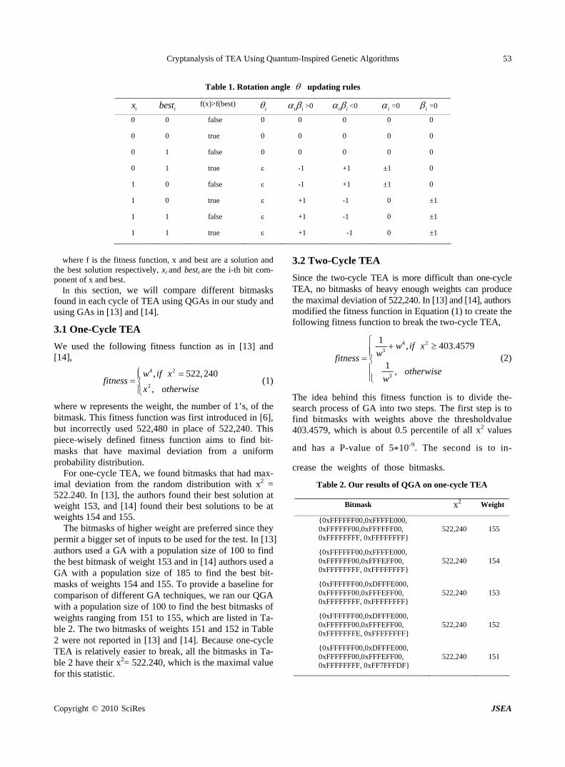
Cryptanalysis of TEA Using Quantum-Inspired Genetic Algorithms
Copyright © 2010 SciRes JSEA
53
Table 1. Rotation angle updating rules
ix ibest f(x)>f(best) i i i >0 i i <0 i =0 i =0
0 0 false 0 0 0 0 0
0 0 true 0 0 0 0 0
0 1 false 0 0 0 0 0
0 1 true ε -1 +1 ±1 0
1 0 false ε -1 +1 ±1 0
1 0 true ε +1 -1 0 ±1
1 1 false ε +1 -1 0 ±1
1 1 true ε +1 -1 0 ±1
3.2 Two-Cycle TEA where f is the fitness function, x and best are a solution and
the best solution respectively, xi and besti are the i-th bit com-ponent of x and best. Since the two-cycle TEA is more difficult than one-cycle
TEA, no bitmasks of heavy enough weights can produce the maximal deviation of 522,240. In [13] and [14], authors
In this section, we will compare different bitmasks found in each cycle of TEA using QGAs in our study and using GAs in [13] and [14]. modified the fitness function in Equation (1) to create the
following fitness function to break the two-cycle TEA, 3.1 One-Cycle TEA
4 23
3
1, 403.4579
1,
w if xwfitness
otherwisew
(2) We used the following fitness function as in [13] and [14],
4 2
2
, 522, 240
,
w if xfitness
x otherwise
(1)
The idea behind this fitness function is to divide the-search process of GA into two steps. The first step is to find bitmasks with weights above the thresholdvalue 403.4579, which is about 0.5 percentile of all x2 values
where w represents the weight, the number of 1’s, of the bitmask. This fitness function was first introduced in [6], but incorrectly used 522,480 in place of 522,240. This piece-wisely defined fitness function aims to find bit-masks that have maximal deviation from a uniform probability distribution.
and has a P-value of 5*10-9. The second is to in-
crease the weights of those bitmasks. For one-cycle TEA, we found bitmasks that had max-
imal deviation from the random distribution with x2 = 522.240. In [13], the authors found their best solution at weight 153, and [14] found their best solutions to be at weights 154 and 155.
Table 2. Our results of QGA on one-cycle TEA
Bitmask x2 Weight
{0xFFFFFF00,0xFFFFE000, 0xFFFFFF00,0xFFFFFF00, 0xFFFFFFFF, 0xFFFFFFFF}
522,240 155
{0xFFFFFF00,0xFFFFE000, 0xFFFFFF00,0xFFFEFF00, 0xFFFFFFFF, 0xFFFFFFFF}
522,240 154
{0xFFFFFF00,0xDFFFE000, 0xFFFFFF00,0xFFFEFF00, 0xFFFFFFFF, 0xFFFFFFFF}
522,240 153
{0xFFFFFF00,0xDFFFE000, 0xFFFFFF00,0xFFFEFF00, 0xFFFFFFFE, 0xFFFFFFFF}
522,240 152
{0xFFFFFF00,0xDFFFE000, 0xFFFFFF00,0xFFFEFF00, 0xFFFFFFFF, 0xFF7FFFDF}
522,240 151
The bitmasks of higher weight are preferred since they permit a bigger set of inputs to be used for the test. In [13] authors used a GA with a population size of 100 to find the best bitmask of weight 153 and in [14] authors used a GA with a population size of 185 to find the best bit-masks of weights 154 and 155. To provide a baseline for comparison of different GA techniques, we ran our QGA with a population size of 100 to find the best bitmasks of weights ranging from 151 to 155, which are listed in Ta-ble 2. The two bitmasks of weights 151 and 152 in Table 2 were not reported in [13] and [14]. Because one-cycle TEA is relatively easier to break, all the bitmasks in Ta-ble 2 have their x2= 522.240, which is the maximal value for this statistic.

Cryptanalysis of TEA Using Quantum-Inspired Genetic Algorithms 54
Table 3. Results of GA on two-cycle TEA in [14]
Weight x2
157 459.6417
155 483.6
158 474.8167
145 486.2333
159 451.3917
158 415.8583
160 422.475
157 435.6833
162 488.3333
159 413.8417
Table 4. Our results of QGA on two-cycle TEA
Bitmask x2 Weight
{0xFFFFD7FF,0xFFDFFBFF,0xFFFCADF9, 0xFFFFFBCF, 0xFFFFFF5E, 0xFFFFFB8B}
611.925 170
{0xFFFFD7FF, xFFDFFBFF,0xFFFCAC75, 0xFFFFDFCF, 0xFFFFFF5E, 0xFFFFFFCB}
606.725 170
{0xFFFFD7F7, 0xFF9FFBFF, 0xFFFEAFF1, 0xFFFFFFCF, 0xFFFFFF5E, 0xFFFFFF8B}
588.875 171
{0xFFFFD7F7,0xFF9FFBFF,0xFFFCBD7B, 0xFFFFFFCF, 0xFFFFFF5E, 0xFFFFFB8F}
572.375 171
{0xFFFFD7FF,0xFF9FFBFF, 0xFFFCAD75, 0xFFFFFBEF, 0xFFFFFF5E, 0xFFFFFF9B}
538.5 171
{0xFFFFD7F7, 0xFF9FFBFF, 0xFFFFAC77, 0xFFFFDFCF, 0xFFFFFF7E, 0xFFFFFF8B}
578.4 171
{0xFFFFD7FF,0xFF9FFBFF, 0xFFFEBDF1, 0xFFFFFBCF, 0xFFFFFF5E, 0xFFFFFB9B}
662.075 171
{0xFFFFD7FF,0xFF9FFBFF, 0xFFFCAD75, 0xFFFFFBEF, 0xFFFFFF5E, 0xFFFFFF9B}
628.125 172
{0xFFFFF7FF,0xFF9FFBFF, 0xFFFCAD73, 0xFFFFFBCF, 0xFFFFF5DE, 0xFFFFFFBF}
635.725 172
{0xFFFFF7F7,0xFFDFFBFF,0xFFFCADF7, 0xFFFFFBCF,0xFFFFFFDF, 0xFFFFFB8B}
598.075 173
In [13], authors employed the fitness function defined
in Equation (2) to find the following best bitmask with a weight of 155 and an average x2 statistic of 508.15 on 30 random input-key datasets:
{0xBFFFF0FA, 0xFFFE7388, 0xFFFFF7F8, 0xFFFFF3F8, 0xFFFFEF85, 0xFFFFEF8C}
In [14] authors found ten bitmasks using the fitness function in Equation (2) and calculated the average x2 statistic across 30 different random input-key datasets, each having 211 input-key pairs. Their results are summa-rized in Table 3.
In [13] and [14], both authors used the same threshold in the fitness function as in Equation (2) for two-cycle, three-cycle, and four-cycle TEAs, and the bitmasks found for four-cycle TEA were not usable due to their
low weights. We suspected that using a different thresh-old in the fitness function for each cycle might be more appropriate since the average x2 values of various cycles are different. Based on this belief, we selected different thresholds in the fitness function for each different cycle.
We used the following fitness function for two-cycle TEA,
4 2
2
, >1100
,
w if xfitness
x otherwise
(3)
The idea behind this fitness function is to ensure the minimum value for x2 first, then find a bitmask of large weight.
Our QGA discovered ten bitmasks whose average x2 statistic across 30 different random input-key datasets and weight are included in Table 4.
In Table 4, the average x2 statistic was 602 and the av-erage bitmask weight was 171, whereas the results from [14] in Table 3 had corresponding values of 453.3875 and 157 respectively.
Our results in Table 4 demonstrated a big improve-ment over those in [13] and [14]. As the cycles of TEA increase, our QGAs show their apparent advantage over GAs as illustrated in the following sections. In all the subsequent experiments below, we used a QGA with population size of 100, generation number of 200, and
0.001 in rotational mutation.
3.3 Three-Cycle TEA
For three-cycle TEA, authors in [14] used the same fit-ness function defined in Equation (2) as for the two-cycle TEA to find ten bitmasks. Their average x2 statistic across 30 different random input-key datasets and weight are presented in Table 5.
In [13], authors used fitness function defined in Equa-tion (2) to get the following best bitmask with a weight of 116 and an average x2 statistic of 466.5 on 30 random input-key datasets:
{0xFFE1F040, 0x FCE70446, 0x FFEFF06E, 0x FFE7F42A, 0x FFBF1825, 0x FFFA0064}
We identified ten bitmasks using the following fitness function for three-cycle TEA,
4 2
2
, >90
,
w if xfitness
0
x otherwise
(4)
The only difference between this function and that in Equation (3) is the threshold employed in the function definition. The information about these bitmasks is summarized in Table 6. The average X
2 statistic was 530.756 and the average bitmask weight was 117.8 in Table 6, while the results from [14] in Table 5 had cor-responding values of 420.8242 and 100.2 respectively.
Copyright © 2010 SciRes JSEA

Cryptanalysis of TEA Using Quantum-Inspired Genetic Algorithms 55
Table 5. Results of GA on three-cycle TEA in [14]
Weight x2
99 427.0
100 432.675
105 413.0417
109 437.7333
104 423.025
93 445.1333
100 396.1917
105 420.7333
79 437.2667
108 375.4417
For two-cycle and three-cycle TEAs, we obtained bet-
ter bitmasks than those found in [13] and [14] in terms of both chi-square statistic and weight.
3.4 Four-Cycle TEA
The task of finding efficient bitmasks becomes more complicated as the cycles of TEA increase. The ap-proaches in [13] and [14] were sufficient to find efficient bitmasks for TEA of cycles less than four, but failed to attack TEA of cycles greater than or equal to four.
In [13], using the fitness function in Equation (2) au-thors found bitmasks of relatively low weights, less than 47. They then took up a different approach. Instead of using chi-square statistic, they used Strict Avalanche Criterion (SAC), a more sensitive measure, to assess the deviation of the output of TEA from randomness. The best bitmask they found was
{0x96922A0C, 0x42C06402, 0x35B11001, 0x97000000, 0xF0000001, 0xBEB00001}
with a weight of 50 and an average x2 statistic of 673.40 on 30 random input-key datasets. Since TEA takes input data of 64 bits, any bitmask of weight less than 64 cannot be useful for different cryptanalysis of TEA.
In [14], authors were unable to find any useful bit-masks for four-cycle TEA. They suspected that with more rounds of calculations in their GA, it might be pos-sible to discover some adequate bitmasks.
Based on the principle that we should approach each cycle differently, the following fitness function was ap-plied to four-cycle TEA,
4 2
2
, >80
,
w if xfitness
0
x otherwise
(5)
Our QGA uncovered five bitmasks. For each of these bitmask, we computed the average x2 statistic across 30 random input-key datasets. The results are listed in Table 7. All these x2 statistic values have a P-value less than 5*10-9.
Table 6. Our results of QGA on three-cycle TEA
Bitmask x2 Weight
{0xF7D65CE6, 0x10FCA894,0xF2ABBFDD, 0xFF0557BB, 0xFF867C02, 0xFFD7E73D}
554.3 120
{0x77D65CE6, 0x10FCA894, 0xF2ABBFDD, 0xFF0557BB, 0xFF867C02, 0xFFD7E73D}
518.74 119
{0x77D65CE6, 0x10FCA894, 0xF2ABBFDD, 0xDF0557BB, 0xFF867C02, 0xFFD7E73D}
536.51 118
{0x77D65CE6, 0x10FCA894, 0xE2ABBFDD, 0xFF0557BB, 0xFF867C02, 0xFBD7E73D}
540.11 117
{0x77D65CE6, 0x10FCA894, 0xE2ABBFDD, 0xDF0557BB, 0xFF867C02, 0xFBD7E73D}
547.80 116
{0xF1729F86, 0x97B6EC6F, 0xFB5A1EE0, 0xFFD328F4, 0xFFE4408C, 0xFFB1FDEA}
542.23 117
{0xF1729F86, 0x97B6EC6F, 0xFB5A1EE0, 0xFFD328F4, 0xFDE4408C, 0xFFB1FDEA}
540.65 116
{0xF38FA5FB, 0xF7E44E4B, 0xF483FB22, 0xF23FE071, 0xFFE1C64D, 0xFFCF5074}
559.45 116
{0xF77C99E2, 0xD157C8BC, 0x7C79BF35, 0x9555D5F2, 0xFFFECA55, 0xCDDDABE5}
482.56 120
{0x773C98EF, 0xD92FCEBC, 0x5C79BF15, 0x955D55F2, 0xFFFECA45, 0xCDDDABC5}
485.21 119
Table 7. Our results of QGA on four-cycle TEA
Bitmask x2 Weight
{0x504007C7, 0xB03C5091, 0x84AE8212, 0x026029C7, 0x411BA198, 0xC81074B8}
740.22 69
{0xF407DC1C, 0x7A123211, 0x8F1042AE, 0x8040A0BE, 0x90017A89, 0x20C204C0}
749.12 69
{ 0x4520B630, 0x0A36E920, 0x0D051868, 0x0AEC3868, 0x2312C768, 0x2460F804}
721.33 69
{0x54D3A2C4, 0x901722EC, 0xE02B0591, 0x21D00283, 0x57848409, 0x49114082}
735.26 67
{0x3E2C642A, 0x80443210, 0xB446B064, 0x87250417, 0x0C93E181, 0x12040508}
767.23 64
The output v[0] & 255 of the first bitmask in Table 7,
from two separate sample runs of TEA on one random input-key dataset of 211 pairs, is displayed in the form of histograms in Figure 1. As illustrated in Figure 1, there is a clear peak or bias at the same position 152 for both runs although the frequencies at all other positions are relatively the same. The x2 statistic values produced by these two sample runs of TEA were 927 and 941 respec-tively. The significance of these x2 statistic values, which measure the deviation of TEA output from randomness, can be evaluated by their P-value. We thought it is more helpful if the plots like those in Figure 1 can be exhib-ited.
3.5 Five-Cycle TEA
In both [13] and [14], no results were reported for five-cycle TEA. We used the following fitness function in this case,
Copyright © 2010 SciRes JSEA
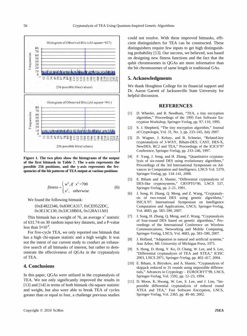
Cryptanalysis of TEA Using Quantum-Inspired Genetic Algorithms 56
Figure 1. The two plots show the histograms of the output of the first bitmask in Table 7. The x-axis represents the possible 256 positions, and the y-axis represents the fre-quencies of the bit patterns of TEA output at various positions
4 2
2
, >70
,
w if xfitness
0
x otherwise
(6)
We found the following bitmask:
{0xE4822346, 0x830CA317, 0xCE9522DC, 0x3E13C130, 0x33C18B0A, 0x128A11A0}
This bitmask has a weight of 76, an average x2 statistic of 631.74 on 30 random input-key datasets, and a P-value less than 5*10-9.
For five-cycle TEA, we only reported one bitmask that has a high chi-square statistic and a high weight. It was not the intent of our current study to conduct an exhaus-tive search of all bitmasks of interest, but rather to dem-onstrate the effectiveness of QGAs in the cryptanalysis of TEA.
4. Conclusions
In this paper, QGAs were utilized in the cryptanalysis of TEA. We not only significantly improved the results in [13] and [14] in terms of both bitmask chi-square statistic and weight, but also were able to break TEA of cycles greater than or equal to four, a challenge previous studies
could not resolve. With these improved bitmasks, effi-cient distinguishers for TEA can be constructed. These distinguishers require few inputs to get high distinguish-ing probability [13]. Our success, we believed, was based on designing new fitness functions and the fact that the qubit chromosomes in QGAs are more informative than the bit chromosomes of same length in traditional GAs. 5. Acknowledgments
We thank Houghton College for its financial support and Dr. Aaron Garrett of Jacksonville State University for helpful discussion.
REFERENCES
[1] D. Wheeler, and R. Needham, “TEA, a tiny encryption algorithm,” Proceedings of the 1995 Fast Software En-cryption Workshop, Springer-Verlag, pp. 97–110, 1995.
[2] S. J. Shepherd, “The tiny encryption algorithm,” Journal of Cryptologia, Vol. 31, No. 3, pp. 233–245, July 2007.
[3] D. Wagner, J. Kelsey, and B. Schneier, “Related-key cryptoanalysis of 3-WAY, Biham-DES, CAST, DES-X, NewDES, RC2 and TEA,” Proceedings of the IClCS’97 Conference, Springer-Verlag, pp. 233–246, 1997.
[4] F. Yang, J. Song, and H. Zhang, “Quantitative cryptana-lysis of six-round DES using evolutionary algorithms,” Proceedings of the 3rd International Symposium on Ad-vances in Computation and Intelligence, LNCS Vol. 5370, Springer-Verlag, pp. 134–141, 2008.
[5] E. Biham and A. Shamir, “Differential cryptanalysis of DES-like cryptosystems,” CRYPTO’90, LNCS 537, Springer-Verlag, pp. 2–21, 1991.
[6] J. Song, H. Zhang, Q. Meng, and Z. Wang, “Cryptanaly-sis of two-round DES using genetic algorithms,” ISICA’07: International Symposium on Intelligence Computation and Applications, LNCS, Springer-Verlag, Vol. 4683, pp. 583–590, 2007.
[7] J. Song, H. Zhang, Q. Meng, and Z. Wang, “Cryptanalysis of four-round DES based on genetic algorithms,” Pro-ceedings of the International Conference on Wireless Communications, Networking and Mobile Computing, Springer-Verlag, LNCS, Vol. 4683, pp. 583–590, 2007.
[8] J. Holland, “Adaptation in natural and artificial systems,” Ann Arbor, MI: University of Michigan Press, 1975.
[9] S. Hong, D. Hong, Y. Ko, D. Chang, W. Lee, and S. Lee, “Differential cryptanalysis of TEA and XTEA,” ICISC 2003, LNCS 2971, Springer-Verlag, pp. 402–417, 2004.
[10] E. Biham, A. Biryukov, and A. Shamir, “Cryptanalysis of skipjack reduced to 31 rounds using impossible differen-tials,” Advances in Cryptology – EUROCRYT’99, LNCS, Springer-Verlag, Vol. 1592, pp. 12–23, 1994.
[11] D. Moon, K. Hwang, W. Lee, S. Lee, and J. Lim, “Im-possible differential cryptanalysis of reduced round XTEA and TEA,” Fast Software Encryption, LNCS, Springer-Verlag, Vol. 2365. pp. 49–60, 2002.
Copyright © 2010 SciRes JSEA

Cryptanalysis of TEA Using Quantum-Inspired Genetic Algorithms
Copyright © 2010 SciRes JSEA
57
[12] L. Knudsen and W. Meier, “Correlations in RC6 with a reduced number of rounds,” Proceedings of the Seventh Fast Software Encryption Workshop, Springer-Verlag, 2000.
[13] J. C. Hernandez and P. Isasi, “Finding efficient distin-guishers for cryptographic mappings, with an application to the block cipher TEA,” Proceedings of the 2003 Con-gress on Evolutionary Computation CEC2003, pp. 341–348, IEEE Press, 2003.
[14] A. Garrett, J. Hamilton, and G. Dozier, “Genetic algorithm techniques for the cryptanalysis of TEA,” International Journal on Intelligent Control and Systems Special Session on Information Assurance. Vol. 12, pp. 325–330, 2007.
[15] J. J. Grefenstette, “Optimization of control parameters for genetic algorithms,” IEEE Transactions on Systems, Man ,
and Cybernetics, Vol. 16, No. 1, pp. 122–128, 1986.
[16] R. Penrose, “Shadows of the mind,” Oxford University Press, 1994.
[17] K. H. Han and J. H. Kim, “Introduction of quantum-inspired evolutionary algorithm,” in Proceedings of the 2002 FIRA Robot World Congress, pp. 243–248, May 2002.
[18] S. Y. Yang and L. C. Jiao, “The quantum evolutionary programming,” Proceedings of the 5th International Con-ference on Computational Intelligence and Multimedia Applications (ICCIMA’03), pp. 362–367, 2003.
[19] National Bureau of Standards, Data Encryption Standard, U.S. Department of Commerce, FIPS, Vol. 46, January 1977.
J. Software Engineering & Applications, 2010, 3: 58-64 doi:10.4236/jsea.2010.31007 Published Online January 2010 (http://www.SciRP.org/journal/jsea)
Copyright © 2010 SciRes JSEA
Application of Design Patterns in Process of Large-Scale Software Evolving Wei WANG, Hai ZHAO, Hui LI, Peng LI, Dong YAO, Zheng LIU, Bo LI, Shuang YU, Hong LIU, Kunzhan YANG
Information Science and Engineering, Northeastern University, Shenyang, China. Email: [email protected], [email protected] Received September 15th, 2009; revised September 29th, 2009; accepted October 13th, 2009.
ABSTRACT
To search for the Design Patterns’ influence on the software, the paper abstracts the feature models of 9 kinds of classic exiting design patterns among the 23 kinds and describes the features with algorithm language. Meanwhile, searching for the specific structure features in the network, the paper designs 9 matching algorithms of the 9 kinds design patterns mentioned above to research on the structure of the design patterns in the software network. At last, the paper analyzes the evolving trends of the software scale and the application frequency of the 9 kinds of design patterns as the software evolves, and search for the rules how these design patterns are applied into 4 kinds of typical software. Keywords: Design Pattern, Feature Model, Software Network, Evolving Trends
1. Introduction
With the increasing of system scale and complexity, the reliability and maintainability are highly required. Design Patterns describe common problems that frequently occur in the process of the object oriented software development and give the resolutions of these problems. Implication Design Patterns into software development can enhance the open, compatibility, stability and exten- sibility of software, which makes the development and maintenance much easier [1].
Does Design Patterns improve the quality of software efficiently? Can Design Patterns be widely used? How these patterns are composed reasonably? What is the reasonable scope of the ratio of the times patterns used and software scale? Facing these questions, it becomes an urgent issue to quantify and measure these patterns when they are used in software in the process of software designing.
If software continues to evolve, it needs to be reor- ganized [2–4]. This is called refactoring and the frames occur during this time. A better understanding of Design Patterns will reduce the time that is spent on refactoring. Looking into how design patterns are implied into some software organized fairly well and evolved continually can direct the design of software system positively. Therefore, it is significant to find out the evolving trends
that design patterns are implied into software designing [5,6].
With the help of open-source software Doxygen, the object oriented software is abstract into XML. Then with the help of XmlParse which is developed in my lab, collect the nodes and edges from XML and abstract the software into software network.
The topology of software system can be represented by topology of network [7–9]. In the network, nodes re- present the component of software and the edges repre- sent the relation between nodes. Complex networks theory is applied into software system which mainly refers to open source software, reverse engineering that get the class graph and network model of the source code is taken to get and analyze the organization structure [10,11]. The abstraction process is shown as Figure 1.
2. Abstracting Process
According to the definition of the design patterns, the paper abstracts the structure features and expresses in mathematical language, which is used for designing and realizing the matching algorithm [12–15].
In the software network, nodes present the abstract data; edges present the relation between the nodes. Nodes can be classified into class, struct and interface; edges can be classified into inherit, usage, static, template and
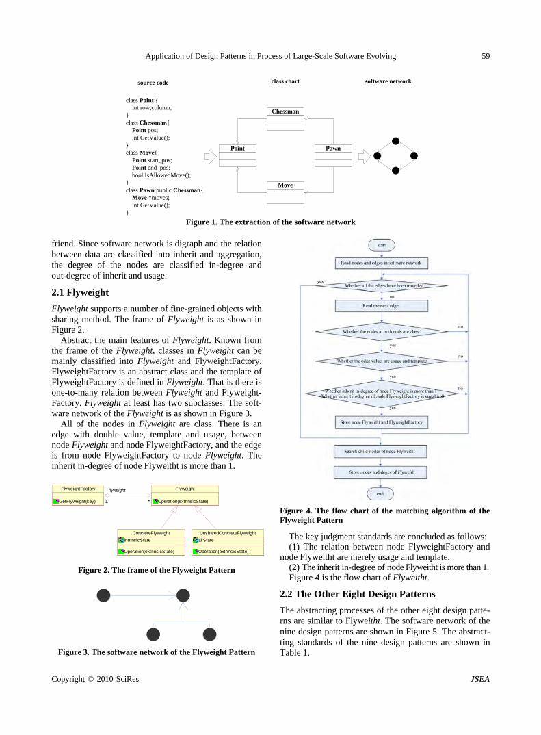
Application of Design Patterns in Process of Large-Scale Software Evolving 59
class Point { int row,column;}class Chessman{
Point pos; int GetValue();}class Move{ Point start_pos; Point end_pos; bool IsAllowedMove();}class Pawn:public Chessman{ Move *moves; int GetValue();}
source code class chart software network
Point
Chessman
Move
Pawn
Figure 1. The extraction of the software network
friend. Since software network is digraph and the relation between data are classified into inherit and aggregation, the degree of the nodes are classified in-degree and out-degree of inherit and usage.
2.1 Flyweight
Flyweight supports a number of fine-grained objects with sharing method. The frame of Flyweight is as shown in Figure 2.
Abstract the main features of Flyweight. Known from the frame of the Flyweight, classes in Flyweight can be mainly classified into Flyweight and FlyweightFactory. FlyweightFactory is an abstract class and the template of FlyweightFactory is defined in Flyweight. That is there is one-to-many relation between Flyweight and Flyweight- Factory. Flyweight at least has two subclasses. The soft- ware network of the Flyweight is as shown in Figure 3.
All of the nodes in Flyweight are class. There is an edge with double value, template and usage, between node Flyweight and node FlyweightFactory, and the edge is from node FlyweightFactory to node Flyweight. The inherit in-degree of node Flyweitht is more than 1.
FlyweightFactory
GetFlyweight(key)
Flyweight
Operation(extrinsicState)1 *1 *
flyweight
ConcreteFlyweight
intrinsicState
Operation(extrinsicState)
UnsharedConcreteFlyweight
allState
Operation(extrinsicState)
Figure 2. The frame of the Flyweight Pattern
Figure 3. The software network of the Flyweight Pattern
Figure 4. The flow chart of the matching algorithm of the Flyweight Pattern
The key judgment standards are concluded as follows: (1) The relation between node FlyweightFactory and
node Flyweitht are merely usage and template. (2) The inherit in-degree of node Flyweitht is more than 1. Figure 4 is the flow chart of Flyweitht.
2.2 The Other Eight Design Patterns
The abstracting processes of the other eight design patte- rns are similar to Flyweitht. The software network of the nine design patterns are shown in Figure 5. The abstract- ting standards of the nine design patterns are shown in Table 1.
Copyright © 2010 SciRes JSEA
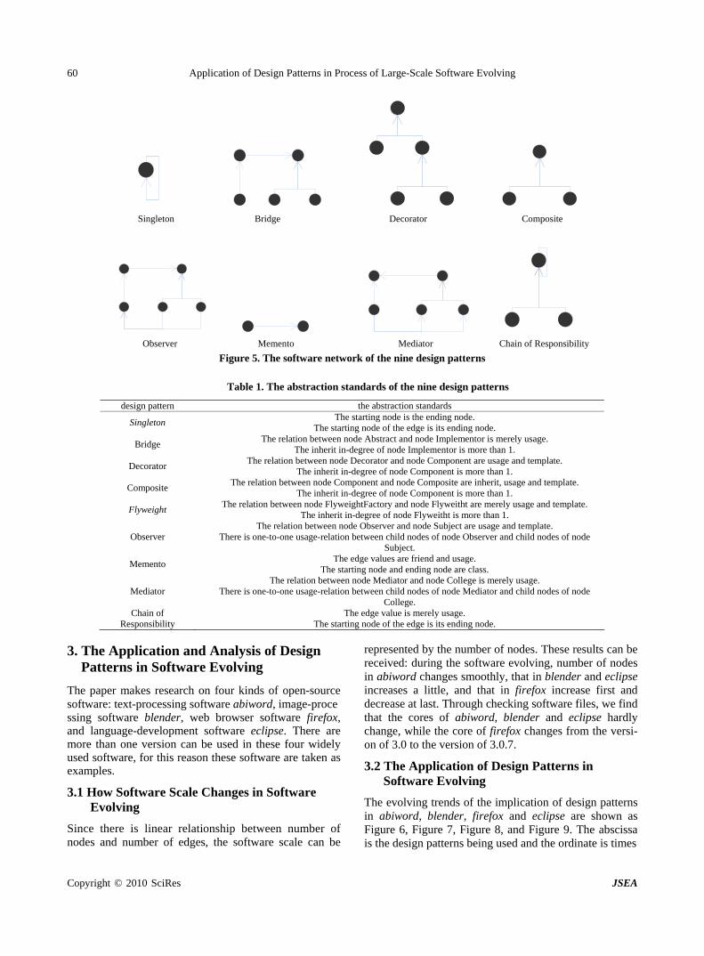
Application of Design Patterns in Process of Large-Scale Software Evolving 60
Singleton Bridge Decorator Composite
Observer Memento Mediator Chain of Responsibility
Figure 5. The software network of the nine design patterns
Table 1. The abstraction standards of the nine design patterns
design pattern the abstraction standards
Singleton The starting node is the ending node.
The starting node of the edge is its ending node.
Bridge The relation between node Abstract and node Implementor is merely usage.
The inherit in-degree of node Implementor is more than 1.
Decorator The relation between node Decorator and node Component are usage and template.
The inherit in-degree of node Component is more than 1.
Composite The relation between node Component and node Composite are inherit, usage and template.
The inherit in-degree of node Component is more than 1.
Flyweight The relation between node FlyweightFactory and node Flyweitht are merely usage and template.
The inherit in-degree of node Flyweitht is more than 1.
Observer The relation between node Observer and node Subject are usage and template.
There is one-to-one usage-relation between child nodes of node Observer and child nodes of node Subject.
Memento The edge values are friend and usage.
The starting node and ending node are class.
Mediator The relation between node Mediator and node College is merely usage.
There is one-to-one usage-relation between child nodes of node Mediator and child nodes of node College.
Chain of Responsibility
The edge value is merely usage. The starting node of the edge is its ending node.
3. The Application and Analysis of Design Patterns in Software Evolving
The paper makes research on four kinds of open-source software: text-processing software abiword, image-proce ssing software blender, web browser software firefox, and language-development software eclipse. There are more than one version can be used in these four widely used software, for this reason these software are taken as examples.
3.1 How Software Scale Changes in Software Evolving
Since there is linear relationship between number of nodes and number of edges, the software scale can be
represented by the number of nodes. These results can be received: during the software evolving, number of nodes in abiword changes smoothly, that in blender and eclipse increases a little, and that in firefox increase first and decrease at last. Through checking software files, we find that the cores of abiword, blender and eclipse hardly change, while the core of firefox changes from the versi- on of 3.0 to the version of 3.0.7.
3.2 The Application of Design Patterns in Software Evolving
The evolving trends of the implication of design patterns in abiword, blender, firefox and eclipse are shown as Figure 6, Figure 7, Figure 8, and Figure 9. The abscissa is the design patterns being used and the ordinate is times
Copyright © 2010 SciRes JSEA
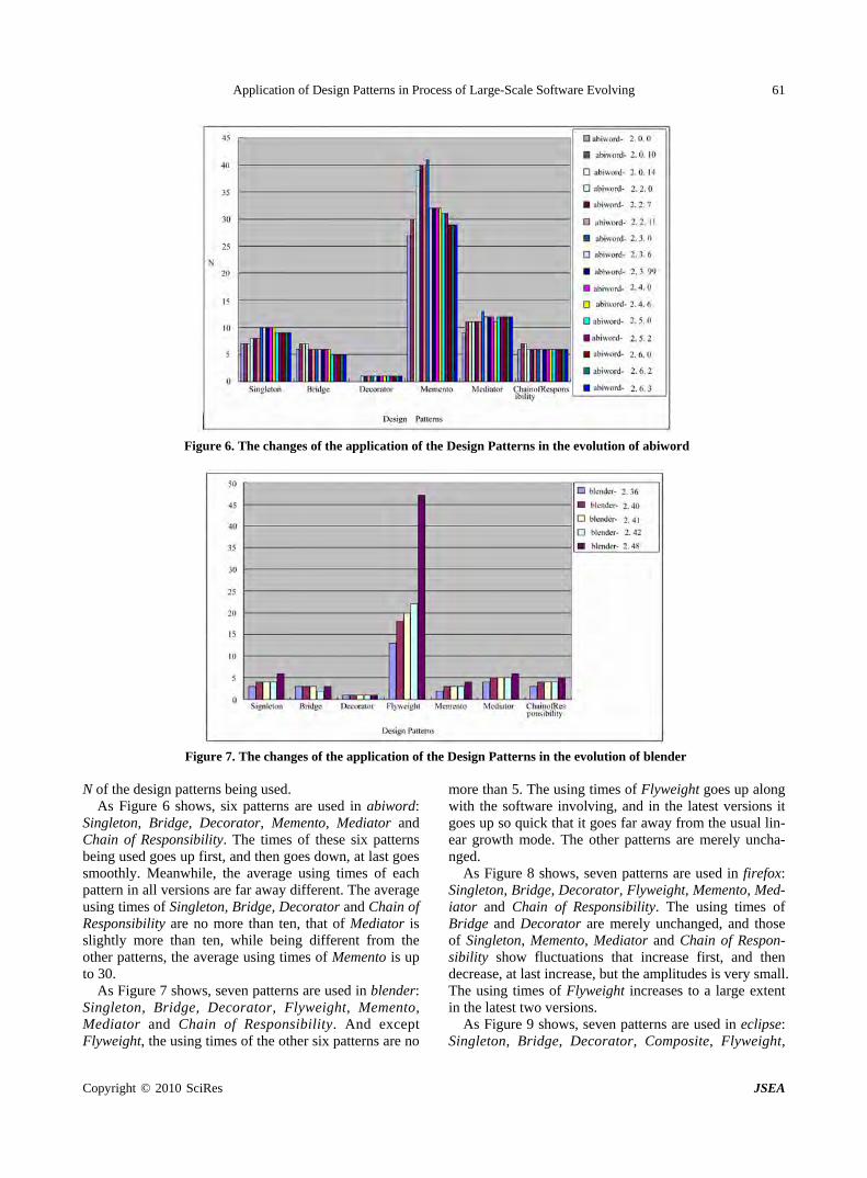
Application of Design Patterns in Process of Large-Scale Software Evolving 61
Figure 6. The changes of the application of the Design Patterns in the evolution of abiword
Figure 7. The changes of the application of the Design Patterns in the evolution of blender
N of the design patterns being used.
As Figure 6 shows, six patterns are used in abiword: Singleton, Bridge, Decorator, Memento, Mediator and Chain of Responsibility. The times of these six patterns being used goes up first, and then goes down, at last goes smoothly. Meanwhile, the average using times of each pattern in all versions are far away different. The average using times of Singleton, Bridge, Decorator and Chain of Responsibility are no more than ten, that of Mediator is slightly more than ten, while being different from the other patterns, the average using times of Memento is up to 30.
As Figure 7 shows, seven patterns are used in blender: Singleton, Bridge, Decorator, Flyweight, Memento, Mediator and Chain of Responsibility. And except Flyweight, the using times of the other six patterns are no
more than 5. The using times of Flyweight goes up along with the software involving, and in the latest versions it goes up so quick that it goes far away from the usual lin- ear growth mode. The other patterns are merely uncha- nged.
As Figure 8 shows, seven patterns are used in firefox: Singleton, Bridge, Decorator, Flyweight, Memento, Med- iator and Chain of Responsibility. The using times of Bridge and Decorator are merely unchanged, and those of Singleton, Memento, Mediator and Chain of Respon- sibility show fluctuations that increase first, and then decrease, at last increase, but the amplitudes is very small. The using times of Flyweight increases to a large extent in the latest two versions.
As Figure 9 shows, seven patterns are used in eclipse: Singleton, Bridge, Decorator, Composite, Flyweight,
Copyright © 2010 SciRes JSEA
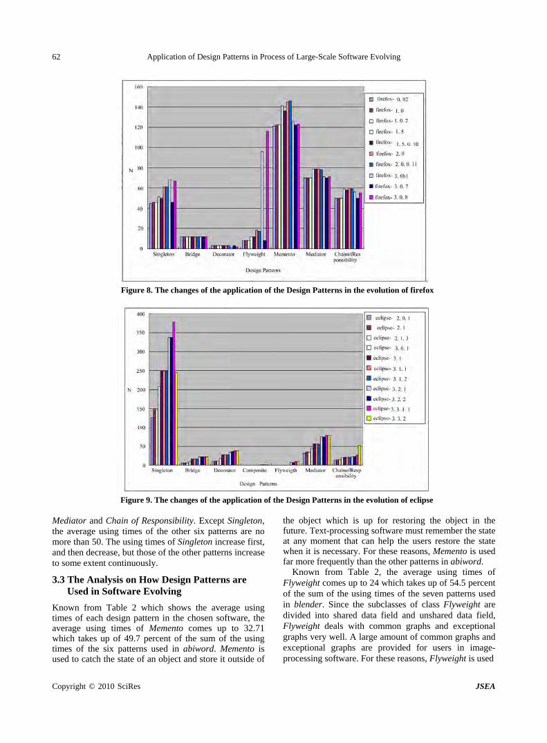
Application of Design Patterns in Process of Large-Scale Software Evolving 62
Figure 8. The changes of the application of the Design Patterns in the evolution of firefox
Figure 9. The changes of the application of the Design Patterns in the evolution of eclipse
Mediator and Chain of Responsibility. Except Singleton, the average using times of the other six patterns are no more than 50. The using times of Singleton increase first, and then decrease, but those of the other patterns increase to some extent continuously.
3.3 The Analysis on How Design Patterns are Used in Software Evolving
Known from Table 2 which shows the average using times of each design pattern in the chosen software, the average using times of Memento comes up to 32.71 which takes up of 49.7 percent of the sum of the using times of the six patterns used in abiword. Memento is used to catch the state of an object and store it outside of
the object which is up for restoring the object in the future. Text-processing software must remember the state at any moment that can help the users restore the state when it is necessary. For these reasons, Memento is used far more frequently than the other patterns in abiword.
Known from Table 2, the average using times of Flyweight comes up to 24 which takes up of 54.5 percent of the sum of the using times of the seven patterns used in blender. Since the subclasses of class Flyweight are divided into shared data field and unshared data field, Flyweight deals with common graphs and exceptional graphs very well. A large amount of common graphs and exceptional graphs are provided for users in image- processing software. For these reasons, Flyweight is used
Copyright © 2010 SciRes JSEA

Application of Design Patterns in Process of Large-Scale Software Evolving 63
Table 2. The average using times of each design pattern in the software
Design Patterns abiword blender firefox eclipse
Singleton 8.75 4.2 54.1 242.8
Bridge 5.875 2.8 12 14.91
Decorator 0.8125 1 2.7 25.64
Composite 0 0 0 0.364
Flyweight 0 24 30.3 3.09
Observer 0 0 0 0
Memento 32.71 3 130.4 0
Mediator 11.5 5 73.7 56.82
Chain of Responsibility 6.125 4 54.7 22.73
far more frequently than the other patterns in blender.
Known from Table 2: the using times of Singleton comes up to 54.1 which takes up of 15.1 percent of the sum of the average using times of the seven patterns used in firefox; the using times of Memento comes up to 130.4 which takes up of 36.4 percent of the sum of the average using times of the seven patterns used in firefox; the using times of Mediator comes up to 73.7 which takes up of 20.6 percent of the sum of the average using times of the seven patterns used in firefox; the using times of Chain of Responsibility comes up to 54.7 which takes up of 15.3 percent of the sum of the average using times of the seven patterns used in firefox. Mediator can deal with the communication among the objects implicitly. Chain of Responsibility can make these requests a line and pass these requests along the line till the final processing. Memento can store the reply data being received for client processing. At the same time, web browser takes C/S model, so users will sent and receive large amount of data request and reply continuously. For these reasons, Memento, Mediator, Chain of Responsibility and Chain of Responsibility are used far more frequently than the other patterns in firefox.
Known from Table 2, the average using times of Singleton comes up to 242.8 which takes up of 66.3 percent of the sum of the using times of the seven patt- erns used in eclipse. The developers have to call the system functions through the interfaces provided by eclipse when they use eclipse and these system interfaces permit being called but not changed, while Singleton can prevent the change made by developers when they use these interfaces. For these reasons, Singleton is used far more frequently than the other patterns in eclipse.
Definition 1: the using times of some design patterns takes up more than 50 percent of the sum of the using times of all the patterns in software, then this pattern is key pattern.
According to the Definition 1, the key pattern of software is similar to the key in database. Since the key pattern decides the main function of software, it can be some kind of symbol of the software. Based on the Definition 1, the key pattern of abiword is Memento; the key pattern of blender is Flyweight; the key patterns of firefox are Memento and Mediator; the key pattern of eclipse is Singleton.
As Figure 6, Figure 7, Figure 8, and Figure 9 show, the using times of Flyweight appears abnormal changes in the last versions of firefox and blender. Through referring to the white books of firefox and blender, we find that the cores of firefox and blender changed too where these abnormal changes happens [16].
4. Conclusions
According what mentioned above, the application and rule of software in the process of evolving is abstracted as follows:
The application of design patterns is changed along with the change of software core and the using times of key pattern of software increases first, then decreases, at last swing around a certain number.
REFERENCES [1] E. Gamma, R. Helm, R. Johnson, and J. Vlissides,
“Design patterns: Elements of reusable object-oriented software [M],” Addison-Wesley Longman Publishing Co., Inc. Boston, MA, USA, 1995.
[2] M. M. Lehma, and J. F. Rmail, “Software evolution and software evolution processes [J],” Annals of Software Engineering, Vol. 14, No. 1, pp. 275–309, 2002.
[3] B. Dougherty, J. White, C. Thompson, and D. C. Schmidt, “Automating hardware and software evolution analysis [A],” Engineering of Computer Based Systems, ECBS 2009. 16th Annual IEEE International Conference and Workshop on the [C], Vol. 35, No. 5, pp. 265–274, 2009.
Copyright © 2010 SciRes JSEA
Application of Design Patterns in Process of Large-Scale Software Evolving64
[4] S. N. Dorogovtsev, and J. F. Mendes, “Scaling properties of scale-free evolving networks: continuous approach [J],” Physical Review E, Vol. 63, No. 5, pp. 56125.
[5] N. Zhao, T. Li, L. L. Yang, Y. Yu, F. Dai, and W. Zhang, “The resource optimization of software evolution processes [A],” Advanced Computer Control, ICACC’09, International Conference on [C], pp. 332–336, 2009.
[6] B. Behm, “Some future trends and implications for systems and software engineering processes [J],” Systems Engineering, Vol. 9, No. 1, pp. 1–19, 2006.
[7] L. Paolo, B. Andrea, and D. G. Felicita, “A decom- position-based modeling framework for complex systems [J],” IEEE Transaction on Reliability, Vol. 58, No. 1, pp. 20–33, 2009.
[8] Y. Ma, and K. A. He, “Complexity metrics set for large-scale object-oriented software systems, in procee- dings of 6th international conference on computer and information technology [J],” pp. 189–189, 2006.
[9] K. Madhavi, and A. A. A. Rao, “Framework for visua- lizing model-driven software evolution [A], Advance Computing Conference IACC’09 IEEE International [C],” pp. 1628–1633, 2009.
[10] S. Valverde, and R. V. Sole, “Network notifs in com-
putational graphs: a case study in software architecture [J],” Physical Review E, Vol. 72, No. 2, pp. 26107, 2005.
[11] C. R. Myers, “Software systems as complex networks: structure, function, and evolvability of software collaboration graphs [J],” Physical Review E, Vol. 68, No. 4, pp. 46116, 2003.
[12] A. Potanin, et al. “Scale-free geometry in OO programs [J],” Communications of ACM, Vol. 48, No. 5, pp. 99–103, 2005.
[13] S. Meyers, “Effective C++ (3rd Edition) [M],” Addison- Wesley Professional, pp. 10–50, 2005.
[14] C. A. Conley, and L. Sproull, “Easier said than done: an empirical investigation of software design and quality in open source software development [A],” System Sciences, HICSS’09 42nd Hawaii International Conference on [C], pp. 1–10, 2009.
[15] W. Lian, R. G. Dromey, and D. Kirk, “Software Engineering and Scale-free Networks [J],” IEEE Trans- actions on Systems, Vol. 39, No. 3, pp. 648–657, 2009.
[16] M. M. Lehma, and J. F. Rmail, “Software evolution background, theory, practice [J],” Information Processing Letters, Vol. 88, No. 1/2, pp. 33–44, 2003.
Copyright © 2010 SciRes JSEA
J. Software Engineering & Applications, 2010, 3: 65-72 doi:10.4236/jsea.2010.31008 Published Online January 2010 (http://www.SciRP.org/journal/jsea)
Copyright © 2010 SciRes JSEA
Element Retrieval Using Namespace Based on Keyword Search over XML Documents
Yang WANG1, Zhikui CHEN1, Xiaodi HUANG2
1School of Software, Dalian University of Technology, Dalian, China; 2School of Computing and Mathematics, Charles Sturt Uni-versity, Australia. Email: [email protected], [email protected], [email protected] Received July 31st, 2009; revised September 12th, 2009; accepted September 22nd, 2009.
ABSTRACT
Querying over XML elements using keyword search is steadily gaining popularity. The traditional similarity measure is widely employed in order to effectively retrieve various XML documents. A number of authors have already proposed different similarity-measure methods that take advantage of the structure and content of XML documents. However, they do not consider the similarity between latent semantic information of element texts and that of keywords in a query. Although many algorithms on XML element search are available, some of them have the high computational complexity due to searching for a huge number of elements. In this paper, we propose a new algorithm that makes use of the se-mantic similarity between elements instead of between entire XML documents, considering not only the structure and content of an XML document, but also semantic information of namespaces in elements. We compare our algorithm with the three other algorithms by testing on real datasets. The experiments have demonstrated that our proposed method is able to improve the query accuracy, as well as to reduce the running time. Keywords: Semantics, Namespace, SVD, Text Matching
1. Introduction
Keyword search querying over XML elements has emer- ged as one of the most effective paradigms in information retrieval. To identify relevant results for an XML key-word query, different approaches lead to various search results in general. Some authors calculated the similarity between the content of XML documents and query, only analyzing the content and structure of XML (e.g., [1–3]). Many algorithms calculate the degree of text of elements matching with the keywords to produce the ranked re-sult-list (e.g., DIL Query processing algorithm [4] and Top-k algorithm [5]). The classical methods focus on TF-IEF formula to calculate the cosine similarity between elements and query (e.g., Tae-Soon Kim et al. [6]; Maria Izabel M et al. [7]; Yun-tao Zhang et al. [8]).
In particular, overlaps of elements in XML documents must be considered. For several overlapping relevant ele- ments, we have to choose which one should be avoided to ensure that users do not see the same information for several times. Su Cheng Haw et al. [9] presented the TwigINLAB algorithm to improve XML Query process-ing. In this paper, we modify it to deal with the elements overlap occurring in keyword search results.
On the basis of previous work, we make the following
contributions in this paper. Firstly, we utilize the seman-tic information of namespaces in elements to filter the relevant components since the text of elements are com-monly related with semantic information of namespace. Secondly, the precision and recall of our algorithm show that the non-text matching but semantic relevant ele-ments with respect to the keyword can be effectively retrieved. Compared with traditional work, our algorithm also shows the better performance on time execution over a large collection of elements.
The rest of this paper is organized as follows: Section 2 introduces the element-rank schema by keyword search. Section 3 presents the Namespace Filter Algorithm (NFA). The experiments on the comparison of NFA and related methods are reported in Section 4. Related work is presented in Section 5, followed by the conclusion.
2. Element-Rank Schema
In this section, we utilize the namespace of elements to describe our element rank schema. Another goal of util-izing namespace is to filter relevant elements with the keyword in a query to reduce time execution compared with traditional algorithms.
Interestingly, namespaces can distinguish different ele-
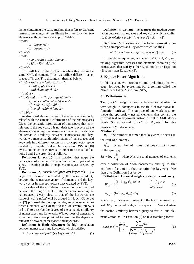
Element Retrieval Using Namespace Based on Keyword Search over XML Documents 66
ments containing the same markup that refers to different semantic meanings. As an illustration, we consider two elements with the same markup of <table>: <table>
<td>apple</td> <td>banana<td>
</table> <table>
<name>coffee table</name> <width>80</width>
</table> This will lead to the confliction when they are in the
same XML document. Thus, we utilize different name-spaces of 'h' and 'f' to distinguish them as below. <h:table xmlns:h = "http://.../fruit">
<h:td>apple</h:td> <h:td>banana</h:td>
</h:table> <f:table xmlns:f = "http://.../furniture">
<f:name>coffee table</f:name> <f:width>80</f:width> <f:length>120</f:length>
</f:table> As discussed above, the text of elements is commonly
related with the semantic information of their namespaces. Given the semantic information of namespace that is ir-relevant to the keyword, it is not desirable to access all the elements containing this namespace. In order to calculate the semantic similarity between namespaces and key-words, we map semantic information of namespaces and keywords into different vectors in a concept vector space created by Singular Value Decomposition (SVD) [10] over a collection of elements. In order to do this, Defini-tions 1 and 2 are provided as follows.
Definition 1: : a function that maps the namespace of element v into a vector and represents a special meaning in the concept vector space created by SVD.
)(vprefix
Definition 2: : the degree of relevance calculated by the cosine similarity between the namespace vector of element v and the key-word vector in concept vector space created by SVD.
)),(( keywordvprefixncorrelatio
The value of the correlation is commonly normalized between the range [-1,1]. If the semantic meaning of namespaces is very close to that of the keywords, the value of ‘correlation’ will be around 1. Nobert Govert et al. [2] proposed the concept of degree of relevance be-tween elements. We extend it to include several intervals in [-1,1] to describe the degree of the semantic similarity of namespaces and keywords. Without loss of generality, some definitions are provided to describe the degree of relevance between namespaces and keywords.
Definition 3: High relevance: the high correlation between namespaces and keywords which satisfies
1)),((1 keywordvprefixncorrelatio (1)
Definition 4: Common relevance: the median corre-lation between namespaces and keywords which satisfies
12 )),(( keywordvprefixncorrelatio (2)
Definition 5: Irrelevance: the lower correlation be-tween namespaces and keywords which satisfies
2)),((1 keywordvprefixncorrelatio (3)
In the above equations, we have 10 12 , our
ranking algorithm accesses the elements containing the namespaces that satisfy either Equation (1) or Equation (2) rather than Equation (3).
3. Espace Filter Algorithm
In this section, we introduce some preliminary knowl-edge, followed by presenting our algorithm called the Namespace Filter Algorithm (NFA).
3.1 Preliminaries
The idftf weight is commonly used to calculate the
term weight in documents in the field of traditional in-formation retrieval. The purpose of our work is to re-trieve the appropriate nested elements that contain the relevant text to keywords instead of entire XML docu-ments. So we extend idftf to for ele-
ments in XML documents.
ieftf et ,
Notations:
ettf , the number of times that keyword t occurs in
the text of element e.
qttf , the number of times that keyword t occurs
in the query q.
ef
Nief 10log where is the total number of elements
over a collection of XML documents, and is the
number of elements that contain the keyword. We then give Definition 6 as below.
N
ef
Definition 6: keyword weights in elements and query
otherwise
tfifieftfW etet
et
0
0)log1( ,,10, (4)
ieftfW qtqt )log1( ,10, (5)
where is keyword weight in the text of element ,
and keyword weight in a query . We calculate
the cosine similarity between query vector
etW ,
qt ,
e
W q
q
and ele-
ment vector e
in Equation (6) on text matching factor.
n
i in
i i
n
i ii
eq
eq
eq
eqeqscore
1
2
1
2
1),( (6)
Copyright © 2010 SciRes JSEA
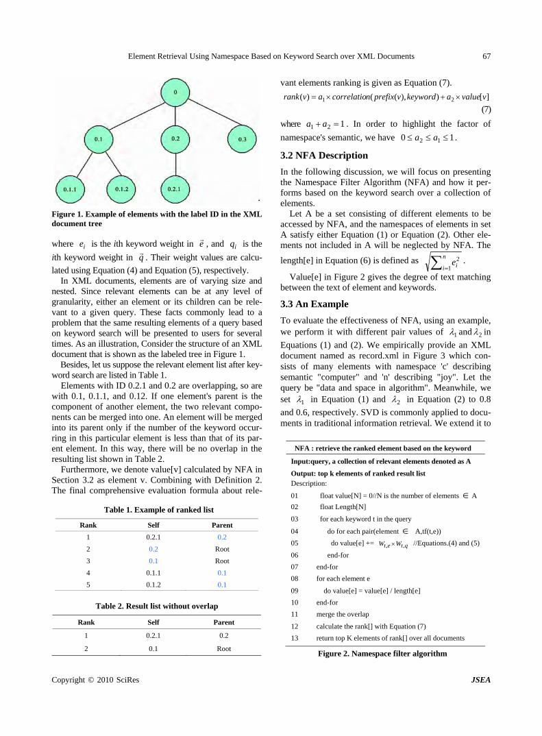
Element Retrieval Using Namespace Based on Keyword Search over XML Documents 67
Figure 1. Example of elements with the label ID in the XML document tree where is the ith keyword weight in ie e
, and is the
ith keyword weight in iq
q
. Their weight values are calcu-
lated using Equation (4) and Equation (5), respectively. In XML documents, elements are of varying size and
nested. Since relevant elements can be at any level of granularity, either an element or its children can be rele-vant to a given query. These facts commonly lead to a problem that the same resulting elements of a query based on keyword search will be presented to users for several times. As an illustration, Consider the structure of an XML document that is shown as the labeled tree in Figure 1.
Besides, let us suppose the relevant element list after key-word search are listed in Table 1.
Elements with ID 0.2.1 and 0.2 are overlapping, so are with 0.1, 0.1.1, and 0.12. If one element's parent is the component of another element, the two relevant compo-nents can be merged into one. An element will be merged into its parent only if the number of the keyword occur-ring in this particular element is less than that of its par-ent element. In this way, there will be no overlap in the resulting list shown in Table 2.
Furthermore, we denote value[v] calculated by NFA in Section 3.2 as element v. Combining with Definition 2. The final comprehensive evaluation formula about rele-
Table 1. Example of ranked list
Rank Self Parent
1 0.2.1 0.2
2 0.2 Root
3 0.1 Root
4 0.1.1 0.1
5 0.1.2 0.1
Table 2. Result list without overlap
Rank Self Parent
1 0.2.1 0.2
2 0.1 Root
vant elements ranking is given as Equation (7).
][)),(()( 21 vvalueakeywordvprefixncorrelatioavrank
(7)
where 121 aa . In order to highlight the factor of
namespace's semantic, we have . 10 12 aa
3.2 NFA Description
In the following discussion, we will focus on presenting the Namespace Filter Algorithm (NFA) and how it per-forms based on the keyword search over a collection of elements.
Let A be a set consisting of different elements to be accessed by NFA, and the namespaces of elements in set A satisfy either Equation (1) or Equation (2). Other ele-ments not included in A will be neglected by NFA. The
length[e] in Equation (6) is defined as
n
i ie1
2 .
Value[e] in Figure 2 gives the degree of text matching between the text of element and keywords.
3.3 An Example
To evaluate the effectiveness of NFA, using an example, we perform it with different pair values of 1 and 2 in
Equations (1) and (2). We empirically provide an XML document named as record.xml in Figure 3 which con-sists of many elements with namespace 'c' describing semantic "computer" and 'n' describing "joy". Let the query be "data and space in algorithm". Meanwhile, we set 1 in Equation (1) and 2 in Equation (2) to 0.8
and 0.6, respectively. SVD is commonly applied to docu- ments in traditional information retrieval. We extend it to
NFA : retrieve the ranked element based on the keyword
Input:query, a collection of relevant elements denoted as A
Output: top k elements of ranked result list Description:
01 float value[N] = 0//N is the number of elements A
02 float Length[N]
03 for each keyword t in the query
04 do for each pair(element A,tf(t,e))
05 do value[e] += //Equations.(4) and (5)qtet WW ,,
06 end-for
07 end-for
08 for each element e
09 do value[e] = value[e] / length[e]
10 end-for
11 merge the overlap
12 calculate the rank[] with Equation (7)
13 return top K elements of rank[] over all documents
Figure 2. Namespace filter algorithm
Copyright © 2010 SciRes JSEA
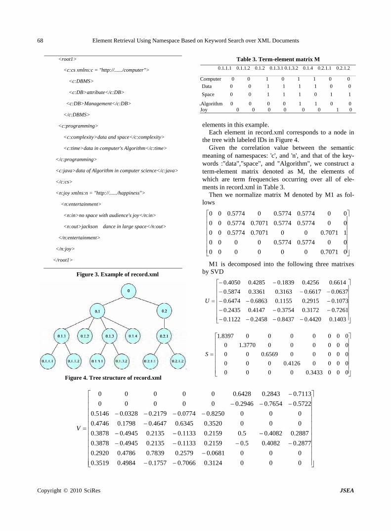
Element Retrieval Using Namespace Based on Keyword Search over XML Documents
Copyright © 2010 SciRes JSEA
68
Table 3. Term-element matrix M <root1>
<c:cs xmlns:c = "http://....../computer">
<c:DBMS>
<c:DB>attribute</c:DB>
<c:DB>Management</c:DB>
</c:DBMS>
<c:programming>
<c:complexity>data and space</c:complexity>
<c:time>data in computer's Algorithm</c:time>
</c:programming>
<c:java>data of Algorithm in computer science</c:java>
</c:cs>
<n:joy xmlns:n = "http://....../happiness">
<n:entertainment>
<n:in>no space with audience's joy</n:in>
<n:out>jackson dance in large space</n:out>
</n:entertainment>
</n:joy>
</root1>
0.1.1.1 0.1.1.2 0.1.2 0.1.3.1 0.1.3.2 0.1.4 0.2.1.1 0.2.1.2
Computer 0 0 1 0 1 1 0 0
Data 0 0 1 1 1 1 0 0
Space 0 0 1 1 1 0 1 1
AAlgorithm 0 0 0 0 1 1 0 0 Joy 0 0 0 0 0 0 1 0
elements in this example.
Each element in record.xml corresponds to a node in the tree with labeled IDs in Figure 4.
Given the correlation value between the semantic meaning of namespaces: 'c', and 'n', and that of the key-words :"data","space", and "Algorithm", we construct a term-element matrix denoted as M, the elements of which are term frequencies occurring over all of ele-ments in record.xml in Table 3.
Then we normalize matrix M denoted by M1 as fol-lows
07071.0000000
005774.05774.00000
17071.0007071.05774.000
005774.05774.07071.05774.000
005774.05774.005774.000
M1 is decomposed into the following three matrixes by SVD Figure 3. Example of record.xml
1403.04420.08437.02458.01122.0
7261.03172.03754.04147.02435.0
1073.02915.01155.06863.06474.0
0637.06617.03163.03361.05874.0
6614.04256.01839.04285.04050.0
U
0003433.00000
00004126.0000
000006569.000
0000003770.10
00000008397.1
S
Figure 4. Tree structure of record.xml
0003124.07066.01757.04984.03519.0
0000681.02579.07839.04786.02920.0
2877.04082.05.02159.01133.02135.04945.03878.0
2887.04082.05.02159.01133.02135.04945.03878.0
0003520.06345.04647.01798.04746.0
0008250.00774.02179.00328.05146.0
5722.07654.02946.000000
7113.02843.06428.000000
V
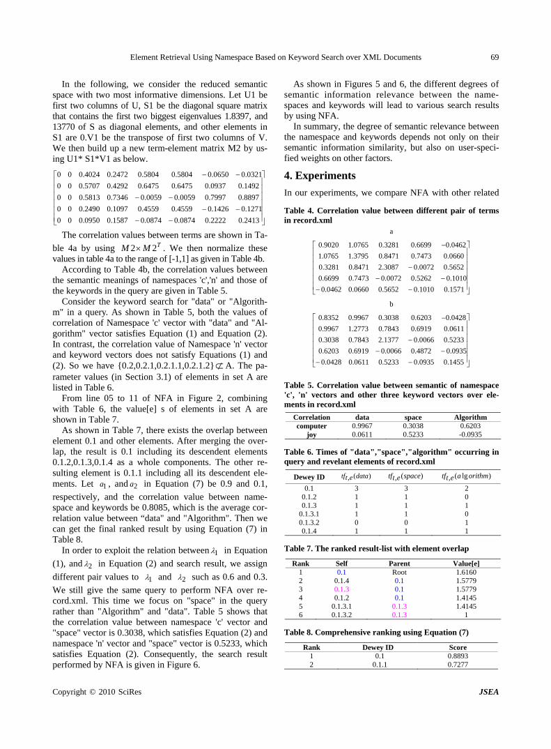
Element Retrieval Using Namespace Based on Keyword Search over XML Documents 69
In the following, we consider the reduced semantic space with two most informative dimensions. Let U1 be first two columns of U, S1 be the diagonal square matrix that contains the first two biggest eigenvalues 1.8397, and 13770 of S as diagonal elements, and other elements in S1 are 0.V1 be the transpose of first two columns of V. We then build up a new term-element matrix M2 by us-ing U1* S1*V1 as below.
2413.02222.00874.00874.01587.00950.000
1271.01426.04559.04559.01097.02490.000
8897.07997.00059.00059.07346.05813.000
1492.00937.06475.06475.04292.05707.000
0321.00650.05804.05804.02472.04024.000
The correlation values between terms are shown in Ta-
ble 4a by using TMM 22 . We then normalize these values in table 4a to the range of [-1,1] as given in Table 4b.
According to Table 4b, the correlation values between the semantic meanings of namespaces 'c','n' and those of the keywords in the query are given in Table 5.
Consider the keyword search for "data" or "Algorith- m" in a query. As shown in Table 5, both the values of correlation of Namespace 'c' vector with "data" and "Al-gorithm" vector satisfies Equation (1) and Equation (2). In contrast, the correlation value of Namespace 'n' vector and keyword vectors does not satisfy Equations (1) and (2). So we have {0.2,0.2.1,0.2.1.1,0.2.1.2}A. The pa-rameter values (in Section 3.1) of elements in set A are listed in Table 6.
From line 05 to 11 of NFA in Figure 2, combining with Table 6, the value[e] s of elements in set A are shown in Table 7.
As shown in Table 7, there exists the overlap between element 0.1 and other elements. After merging the over-lap, the result is 0.1 including its descendent elements 0.1.2,0.1.3,0.1.4 as a whole components. The other re-sulting element is 0.1.1 including all its descendent ele-ments. Let , and in Equation (7) be 0.9 and 0.1,
respectively, and the correlation value between name-space and keywords be 0.8085, which is the average cor-relation value between “data" and "Algorithm". Then we can get the final ranked result by using Equation (7) in Table 8.
1a 2a
In order to exploit the relation between in Equation
(1), and in Equation (2) and search result, we assign
different pair values to and such as 0.6 and 0.3.
We still give the same query to perform NFA over re-cord.xml. This time we focus on "space" in the query rather than "Algorithm" and "data". Table 5 shows that the correlation value between namespace 'c' vector and "space" vector is 0.3038, which satisfies Equation (2) and namespace 'n' vector and "space" vector is 0.5233, which satisfies Equation (2). Consequently, the search result performed by NFA is given in Figure 6.
1
2
1 2
As shown in Figures 5 and 6, the different degrees of semantic information relevance between the name-spaces and keywords will lead to various search results by using NFA.
In summary, the degree of semantic relevance between the namespace and keywords depends not only on their semantic information similarity, but also on user-speci-fied weights on other factors.
4. Experiments
In our experiments, we compare NFA with other related
Table 4. Correlation value between different pair of terms in record.xml
a
1571.01010.05652.00660.00462.0
1010.05262.00072.07473.06699.0
5652.00072.03087.28471.03281.0
0660.07473.08471.03795.10765.1
0462.06699.03281.00765.19020.0
b
1455.00935.05233.00611.00428.0
0935.04872.00066.06919.06203.0
5233.00066.01377.27843.03038.0
0611.06919.07843.02773.19967.0
0428.06203.03038.09967.08352.0
Table 5. Correlation value between semantic of namespace 'c', 'n' vectors and other three keyword vectors over ele-ments in record.xml
Correlation data space Algorithm computer 0.9967 0.3038 0.6203
joy 0.0611 0.5233 -0.0935
Table 6. Times of "data","space","algorithm" occurring in query and revelant elements of record.xml
Dewey ID )(, dataettf )(, spaceettf )lg(, orithmaettf
0.1 3 3 2 0.1.2 1 1 0 0.1.3 1 1 1
0.1.3.1 1 1 0 0.1.3.2 0 0 1 0.1.4 1 1 1
Table 7. The ranked result-list with element overlap
Rank Self Parent Value[e] 1 0.1 Root 1.6160 2 0.1.4 0.1 1.5779 3 0.1.3 0.1 1.5779 4 0.1.2 0.1 1.4145 5 0.1.3.1 0.1.3 1.4145 6 0.1.3.2 0.1.3 1
Table 8. Comprehensive ranking using Equation (7)
Rank Dewey ID Score 1 0.1 0.8893 2 0.1.1 0.7277
Copyright © 2010 SciRes JSEA
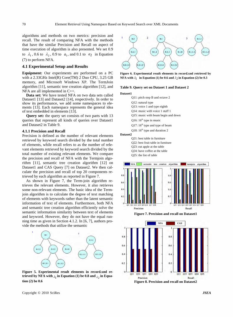
Element Retrieval Using Namespace Based on Keyword Search over XML Documents 70
algorithms and methods on two metrics: precision and recall. The result of comparing NFA with the methods that have the similar Precision and Recall on aspect of time execution of algorithm is also presented. We set 0.9 to 1 , 0.6 to 2 , 0.9 to , and 0.1 to in Equation
(7) to perform NFA. 1a 2a
4.1 Experimental Setup and Results
Equipment: Our experiments are performed on a PC with a 2.33GHz Intel(R) Core(TM) 2 Duo CPU, 3.25 GB memory, and Microsoft Windows XP. The TermJoin algorithm [11], semantic tree creation algorithm [12], and NFA are all implemented in C++.
Data set: We have tested NFA on two data sets called Dataset1 [13] and Dataset2 [14], respectively. In order to show its performance, we add some namespaces to ele-ments [13]. Each namespace represents the general idea of text embedded in elements [13].
Query set: the query set consists of two parts with 13 queries that represent all kinds of queries over Dataset1 and Dataset2 in Table 9.
4.1.1 Precision and Recall Precision is defined as the number of relevant elements retrieved by keyword search divided by the total number of elements, while recall refers to as the number of rele-vant elements retrieved by keyword search divided by the total number of existing relevant elements. We compare the precision and recall of NFA with the Termjoin algo-rithm [11], semantic tree creation algorithm [12] on Dataset1 and CAS Query [7] on Dataset2. We then cal-culate the precision and recall of top 20 components re-trieved by each algorithm as reported in Figure 7.
As shown in Figure 7, the Term-join algorithm re-trieves the relevant elements. However, it also retrieves some non-relevant elements. The basic idea of the Term- join algorithm is to calculate the degree of text matching of elements with keywords rather than the latent semantic information of text of elements. Furthermore, both NFA and semantic tree creation algorithm efficiently solve the semantic information similarity between text of elements and keyword. However, they do not have the equal run-ning time as given in Section 4.1.2. In [6, 7], authors pro-vide the methods that utilize the semantic
Figure 5. Experimental result elements in record.xml re-trieved by NFA with in Equation (1) be 0.8 and in Equa-
tion (2) be 0.6 1 2
Figure 6. Experimental result elements in record.xml retrieved by NFA with in Equation (1) be 0.6 and in Equation (2) be 0.3 1 2
Table 9. Query set on Dataset 1 and Dataset 2
Dataset1 Q11: pitch step B and octave 2
Q12: natural type Q13: voice 1 and type eighth
Q14: music with voice 1 staff 1 Q15: music with beam begin and down
Q16: 16th type in music
Q17: 16th type and type of beam
Q18: 16th type and duration 2 Dataset2
Q21: best table in furniture Q22: best fruit table in furniture Q23: eat apple at the table Q24: have coffee at the table Q25: the list of table
Figure 7. Precision and recall on Dataset1
Figure 8. Precision and recall on Dataset2
Copyright © 2010 SciRes JSEA
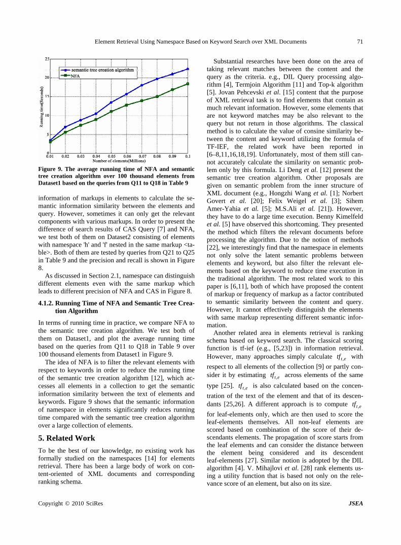
Element Retrieval Using Namespace Based on Keyword Search over XML Documents 71
Figure 9. The average running time of NFA and semantic
formation of markups in elements to calculate the se-
ussed in Section 2.1, namespace can distinguish di
In term e in practice, we compare NFA to
ts with re
knowledge, no existing work has
earches have been done on the area of ta
er related area in elements retrieval is ranking sc
the
tree creation algorithm over 100 thousand elements from Dataset1 based on the queries from Q11 to Q18 in Table 9 inmantic information similarity between the elements and query. However, sometimes it can only get the relevant components with various markups. In order to present the difference of search results of CAS Query [7] and NFA, we test both of them on Dataset2 consisting of elements with namespace 'h' and 'f' nested in the same markup <ta-ble>. Both of them are tested by queries from Q21 to Q25 in Table 9 and the precision and recall is shown in Figure 8.
As discfferent elements even with the same markup which
leads to different precision of NFA and CAS in Figure 8.
4.1.2. Running Time of NFA and Semantic Tree Crea-tion Algorithm
s of running timthe semantic tree creation algorithm. We test both of them on Dataset1, and plot the average running time based on the queries from Q11 to Q18 in Table 9 over 100 thousand elements from Dataset1 in Figure 9.
The idea of NFA is to filter the relevant elemenspect to keywords in order to reduce the running time
of the semantic tree creation algorithm [12], which ac-cesses all elements in a collection to get the semantic information similarity between the text of elements and keywords. Figure 9 shows that the semantic information of namespace in elements significantly reduces running time compared with the semantic tree creation algorithm over a large collection of elements.
5. Related Work
To be the best of ourformally studied on the namespaces [14] for elements retrieval. There has been a large body of work on con-tent-oriented of XML documents and corresponding ranking schema.
Substantial resking relevant matches between the content and the
query as the criteria. e.g., DIL Query processing algo-rithm [4], Termjoin Algorithm [11] and Top-k algorithm [5]. Jovan Pehcevski et al. [15] content that the purpose of XML retrieval task is to find elements that contain as much relevant information. However, some elements that are not keyword matches may be also relevant to the query but not return in those algorithms. The classical method is to calculate the value of consine similarity be-tween the content and keyword utilizing the formula of TF-IEF, the related work have been reported in [6–8,11,16,18,19]. Unfortunately, most of them still can-not accurately calculate the similarity on semantic prob-lem only by this formula. Li Deng et al. [12] present the semantic tree creation algorithm. Other proposals are given on semantic problem from the inner structure of XML document (e.g., Hongzhi Wang et al. [1]; Norbert Govert et al. [20]; Felix Weigel et al. [3]; Sihem Amer-Yahia et al. [5]; M.S.Ali et al. [21]). However, they have to do a large time execution. Benny Kimelfeld et al. [5] have observed this shortcoming. They presented the method which filters the relevant documents before processing the algorithm. Due to the notion of methods [22], we interestingly find that the namespace in elements not only solve the latent semantic problems between elements and keyword, but also filter the relevant ele-ments based on the keyword to reduce time execution in the traditional algorithm. The most related work to this paper is [6,11], both of which have proposed the content of markup or frequency of markup as a factor contributed to semantic similarity between the content and query. However, It cannot effectively distinguish the elements with same markup representing different semantic infor-mation.
Anothhema based on keyword search. The classical scoring
function is tf-ief (e.g., [5,23]) in information retrieval. However, many approaches simply calculate ettf , with
respect to all elements of the collection [9] or p con-sider it by estimating ettf , across elements of the same
type [25]. ettf , is also calculated based on the concen-
tration of th xt of the element and that of its descen-dants [25,26]. A different approach is to compute ettf ,
for leaf-elements only, which are then used to score leaf-elements themselves. All non-leaf elements are scored based on combination of the score of their de-scendants elements. The propagation of score starts from the leaf elements and can consider the distance between the element being considered and its descendent leaf-elements [27]. Similar notion is adopted by the DIL algorithm [4]. V. Mihajlovi et al. [28] rank elements us-ing a utility function that is based not only on the rele-vance score of an element, but also on its size.
artly
e te
Copyright © 2010 SciRes JSEA
Element Retrieval Using Namespace Based on Keyword Search over XML Documents
Copyright © 2010 SciRes JSEA
72
s the keyword search over elem
nymous reviewers for their
REFERENCES [1] H. Z. Wang, J X. M. Lin, “Cod
uhr, and M. Lalmas, “Evalua
gasundaram,
A. Marian, D. Srivastava, and D
Lee, J. W. Song, and D. H. Kim, “Similar-
g, and Y. C. Wang, “An improved
aw and C. S. Lee, “TwigINLAB: A decomposi-
Schutze,” Introduc-
C. Yu, and H. V. Jagadish, “Querying
oral
cxml.org/xml/elite.xml.
www.w3schools.
[15] “HixEval: Highlighting
ring similarity of
, G. Lin, C. Botev, and J. Shanmugasundaram,
“XML
“A novel method for
onsens, and M. Lalmas, “Structural
, Y. Sagiv, and D. Yahav, “Using
anmugasundaram, “Context-sensitive
ct
XXL
. Callan, “Parameter estimation for a sim-
t XML,” IR at INEX 2005.
6. Conclusions
This paper addresse ents tion to information retrieval,” Cambridge Press, April, 2008.
[11] S. Al-Khalifa, in XML documents. Using the namespaces of elements, we have presented the Namespace Filter Algorithm (NFA) that retrieves the relevant components of XML docu-ments with respect to keyword queries. In addition, we provide a new approach that can remove effectively the element overlaps occurring in query results. Using an evaluation formula, our approach is able to produce a ranking result-list without element overlaps. Compared with previous algorithms, NFA has demonstrated a better performance not only on time execution but also on the precision and recall of query results. Our future work will study the relation of the previous factors on the back-ground of graph structures in XML documents.
7. Acknowledgments
We are grateful to the ano
stru
helpful comments.
. Z. Li, W. Wang, and -
sem
ing-based join algorithm for structure queries on graph-structured XML document,” World Wide Web, Vol. 11, pp. 485–510, 2008.
[2] N. Govert, G. Kazai, N. F ting retrieval: What about using contextualrelevance?” SAC, pp. 1114–1115, April 23–27, 2006.
[20] B. Jeong, D. Lee, H. Cho, and J. Lee,the effectiveness of content-oriented XML retrieval,” In-formation Retrieval, Vol. 9, No. 6, pp. 699–722, 2006.
[3] F. Weigel, H. Meuss, and K. U. Schulz, “Francois bry me
content and structure in indexing and ranking XML,” WebDB, Vol. 17–18, pp. 68–72, June 2004.
[4] G. Lin, S. Feng, C. Botev, and J. Shanmu“XRank: Ranked keyword search over XML documents,” ACM International Conference Proceeding, SIGMOD, pp. 7–11, June 9–12, 2003.
[5] S. A. Yahia, N. Koudas, .
rel
Toman, “Structure and content scoring for XML,” Pro-ceedings of the 31st VLDB Conference, pp. 362–372, 2005.
[6] T. S. Kim, J. H. ity measurement of XML documents based on structure and contents,” International Conference on Computational Science (ICCS), Part 3, LNCS 4489, pp. 902–905, 2007.
[7] M. Izabel, M. Azevedo, L. P. Amorim, and N. Ziviani, “A
of st
universal model for XML information retrieval,” LNCS pp. 312–318, 2005.
[8] Y. T. Zhang, L. GonTF-IDF approach for text classification,” Journal of Zhejiang University Science, Vol. 6A, No. 1, pp. 49–55, 2005.
[9] S. C. Htion-matching-merging approach to improving XML query processing,” American Journal of Applied Sciences, Vol. 5, No. 9, pp. 1199–1205, 2008.
[10] C. D. Manning, P. Raghavan, and H.
structured text in an XML database,” ACM International Conference Proceeding, SIGMOD, June 9–12, 2003.
[12] D. Li, X. J. Wang, and L. H. Wang, “Indexing tempXML using semantic tree index,” IEEE Xplore, pp. 448– 451, 2008.
[13] http://www.musi
[14] Namespaces in XML Available: http://com/XML/xml_namespaces.asp/.
J. Pehcevski and J. A. Thom, XML retrieval evaluation,” LNCS 3977, pp. 43–57, 2006.
[16] T. S. Kim, J. H. Lee, J. W. Song, and S. L. Lee, “Semantic ctural similarity for clustering XML documents,” Inha
University Technical Report, 2006. http://webbase.inha. ac.kr/TechnicalReport/tech_04.pdf.
[17] C. Yang and N. Liu, “Measui-structured documents with context weights,” ACM
International Conference Proceeding, pp. 719–720, Au-gust 6–11, 2006.
[18] S. Feng“Efficient keyword search over virtual XML views,” VLDB, pp. 1057–1065, September 23–28, 2007.
[19] K. Sauvagnat, L. Hlaoua, and M. Boughanem,
asuring semantic similarity for XML schema match-ing,” Expert Systems with Applications, Vol. 24, pp. 1651–1658, 2008.
[21] M. S. Ali, M. P. Cevance in XML retrieval evaluation,” Proceedings of
the SIGIR Workshop on XML and Information Retrieval, pp. 2–8, July 27, 2007.
[22] B. Kimelfeld, E. Kovacslanguage models and the HITS algorithm for XML re-trieval,” LNCS 4518, Springer-Verlag Berlin Heidelberg, pp. 253–260, 2007.
[23] C. Botev and J. Shkeyword search and ranking for XML,” WebDB, 2005.
[24] B. Sigurbjornsson, J. Kamps, and M. de Rijke, “The effeructured Queries and selective Indexing on XML re-
trieval,” INEX’05, LNCS 3977, pp. 104–118, 2006.
[25] M. Theobald, R. Schenkel, and G. Weikum, TopX & at INEX 2005.
[26] P. Ogilvie and Jple hierarchical generative model for XML component re-trieval,” INEX, 2004.
[27] S. Geva, “GPX-gardens poin
[28] V. Mihajlovic, G. Ramirez, T. Westerveld, D. Hiemstra, H. E. Blok, and A. P. de Vries, “Vague element selection, image search, overlap, and relevance feedback,” INEX 2005.
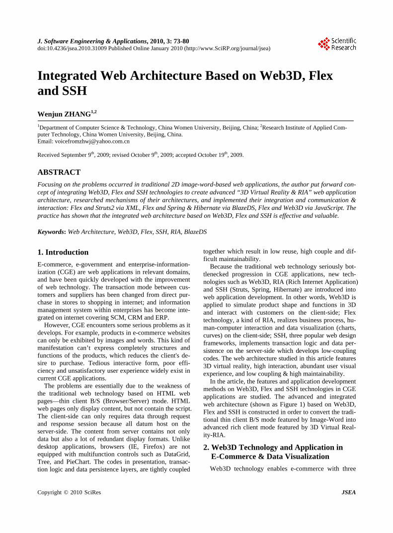
J. Software Engineering & Applications, 2010, 3: 73-80 doi:10.4236/jsea.2010.31009 Published Online January 2010 (http://www.SciRP.org/journal/jsea)
Copyright © 2010 SciRes JSEA
Integrated Web Architecture Based on Web3D, Flex and SSH
Wenjun ZHANG1,2
1Department of Computer Science & Technology, China Women University, Beijing, China; 2Research Institute of Applied Com-puter Technology, China Women University, Beijing, China. Email: [email protected] Received September 9th, 2009; revised October 9th, 2009; accepted October 19th, 2009.
ABSTRACT
Focusing on the problems occurred in traditional 2D image-word-based web applications, the author put forward con-cept of integrating Web3D, Flex and SSH technologies to create advanced “3D Virtual Reality & RIA” web application architecture, researched mechanisms of their architectures, and implemented their integration and communication & interaction: Flex and Struts2 via XML, Flex and Spring & Hibernate via BlazeDS, Flex and Web3D via JavaScript. The practice has shown that the integrated web architecture based on Web3D, Flex and SSH is effective and valuable. Keywords: Web Architecture, Web3D, Flex, SSH, RIA, BlazeDS
1. Introduction
E-commerce, e-government and enterprise-information- ization (CGE) are web applications in relevant domains, and have been quickly developed with the improvement of web technology. The transaction mode between cus-tomers and suppliers has been changed from direct pur-chase in stores to shopping in internet; and information management system within enterprises has become inte-grated on internet covering SCM, CRM and ERP.
However, CGE encounters some serious problems as it develops. For example, products in e-commerce websites can only be exhibited by images and words. This kind of manifestation can’t express completely structures and functions of the products, which reduces the client's de-sire to purchase. Tedious interactive form, poor effi-ciency and unsatisfactory user experience widely exist in current CGE applications.
The problems are essentially due to the weakness of the traditional web technology based on HTML web pages—thin client B/S (Browser/Server) mode. HTML web pages only display content, but not contain the script. The client-side can only requires data through request and response session because all datum host on the server-side. The content from server contains not only data but also a lot of redundant display formats. Unlike desktop applications, browsers (IE, Firefox) are not equipped with multifunction controls such as DataGrid, Tree, and PieChart. The codes in presentation, transac-tion logic and data persistence layers, are tightly coupled
together which result in low reuse, high couple and dif-ficult maintainability.
Because the traditional web technology seriously bot-tlenecked progression in CGE applications, new tech-nologies such as Web3D, RIA (Rich Internet Application) and SSH (Struts, Spring, Hibernate) are introduced into web application development. In other words, Web3D is applied to simulate product shape and functions in 3D and interact with customers on the client-side; Flex technology, a kind of RIA, realizes business process, hu- man-computer interaction and data visualization (charts, curves) on the client-side; SSH, three popular web design frameworks, implements transaction logic and data per-sistence on the server-side which develops low-coupling codes. The web architecture studied in this article features 3D virtual reality, high interaction, abundant user visual experience, and low coupling & high maintainability.
In the article, the features and application development methods on Web3D, Flex and SSH technologies in CGE applications are studied. The advanced and integrated web architecture (shown as Figure 1) based on Web3D, Flex and SSH is constructed in order to convert the tradi-tional thin client B/S mode featured by Image-Word into advanced rich client mode featured by 3D Virtual Real-ity-RIA.
2. Web3D Technology and Application in E-Commerce & Data Visualization
Web3D technology enables e-commerce with three
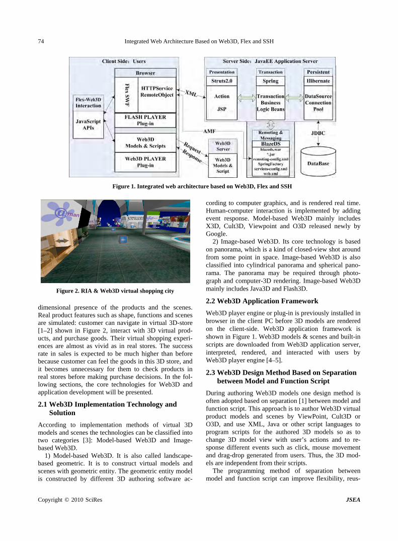
Integrated Web Architecture Based on Web3D, Flex and SSH 74
Figure 1. Integrated web architecture based on Web3D, Flex and SSH
Figure 2. RIA & Web3D virtual shopping city
dimensional presence of the products and the scenes. Real product features such as shape, functions and scenes are simulated: customer can navigate in virtual 3D-store [1–2] shown in Figure 2, interact with 3D virtual prod-ucts, and purchase goods. Their virtual shopping experi-ences are almost as vivid as in real stores. The success rate in sales is expected to be much higher than before because customer can feel the goods in this 3D store, and it becomes unnecessary for them to check products in real stores before making purchase decisions. In the fol-lowing sections, the core technologies for Web3D and application development will be presented.
2.1 Web3D Implementation Technology and Solution
According to implementation methods of virtual 3D models and scenes the technologies can be classified into two categories [3]: Model-based Web3D and Image- based Web3D.
1) Model-based Web3D. It is also called landscape- based geometric. It is to construct virtual models and scenes with geometric entity. The geometric entity model is constructed by different 3D authoring software ac-
cording to computer graphics, and is rendered real time. Human-computer interaction is implemented by adding event response. Model-based Web3D mainly includes X3D, Cult3D, Viewpoint and O3D released newly by Google.
2) Image-based Web3D. Its core technology is based on panorama, which is a kind of closed-view shot around from some point in space. Image-based Web3D is also classified into cylindrical panorama and spherical pano-rama. The panorama may be required through photo-graph and computer-3D rendering. Image-based Web3D mainly includes Java3D and Flash3D.
2.2 Web3D Application Framework
Web3D player engine or plug-in is previously installed in browser in the client PC before 3D models are rendered on the client-side. Web3D application framework is shown in Figure 1. Web3D models & scenes and built-in scripts are downloaded from Web3D application server, interpreted, rendered, and interacted with users by Web3D player engine [4–5].
2.3 Web3D Design Method Based on Separation between Model and Function Script
During authoring Web3D models one design method is often adopted based on separation [1] between model and function script. This approach is to author Web3D virtual product models and scenes by ViewPoint, Cult3D or O3D, and use XML, Java or other script languages to program scripts for the authored 3D models so as to change 3D model view with user’s actions and to re-sponse different events such as click, mouse movement and drag-drop generated from users. Thus, the 3D mod-els are independent from their scripts.
The programming method of separation between model and function script can improve flexibility, reus-
Copyright © 2010 SciRes JSEA
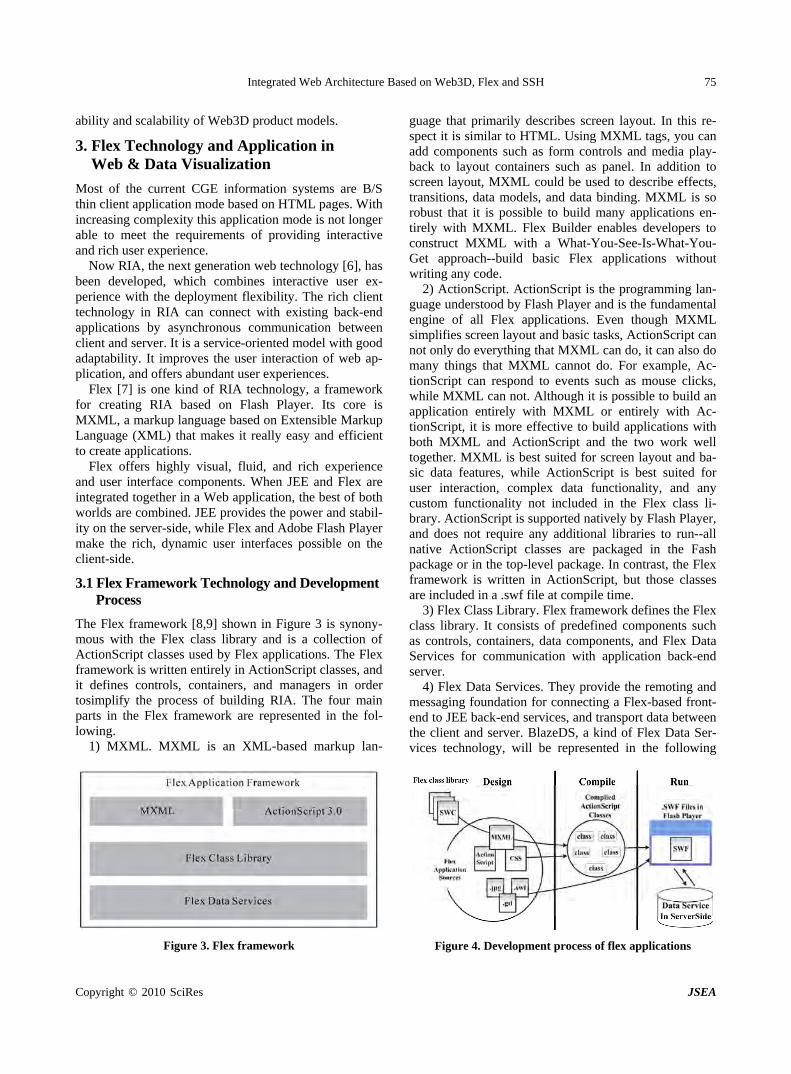
Integrated Web Architecture Based on Web3D, Flex and SSH 75
ability and scalability of Web3D product models.
3. Flex Technology and Application in Web & Data Visualization
Most of the current CGE information systems are B/S thin client application mode based on HTML pages. With increasing complexity this application mode is not longer able to meet the requirements of providing interactive and rich user experience.
Now RIA, the next generation web technology [6], has been developed, which combines interactive user ex-perience with the deployment flexibility. The rich client technology in RIA can connect with existing back-end applications by asynchronous communication between client and server. It is a service-oriented model with good adaptability. It improves the user interaction of web ap-plication, and offers abundant user experiences.
Flex [7] is one kind of RIA technology, a framework for creating RIA based on Flash Player. Its core is MXML, a markup language based on Extensible Markup Language (XML) that makes it really easy and efficient to create applications.
Flex offers highly visual, fluid, and rich experience and user interface components. When JEE and Flex are integrated together in a Web application, the best of both worlds are combined. JEE provides the power and stabil-ity on the server-side, while Flex and Adobe Flash Player make the rich, dynamic user interfaces possible on the client-side.
3.1 Flex Framework Technology and Development Process
The Flex framework [8,9] shown in Figure 3 is synony-mous with the Flex class library and is a collection of ActionScript classes used by Flex applications. The Flex framework is written entirely in ActionScript classes, and it defines controls, containers, and managers in order tosimplify the process of building RIA. The four main parts in the Flex framework are represented in the fol-lowing. 1) MXML. MXML is an XML-based markup lan-
Figure 3. Flex framework
guage that primarily describes screen layout. In this re-spect it is similar to HTML. Using MXML tags, you can add components such as form controls and media play-back to layout containers such as panel. In addition to screen layout, MXML could be used to describe effects, transitions, data models, and data binding. MXML is so robust that it is possible to build many applications en-tirely with MXML. Flex Builder enables developers to construct MXML with a What-You-See-Is-What-You- Get approach--build basic Flex applications without writing any code.
2) ActionScript. ActionScript is the programming lan-guage understood by Flash Player and is the fundamental engine of all Flex applications. Even though MXML simplifies screen layout and basic tasks, ActionScript can not only do everything that MXML can do, it can also do many things that MXML cannot do. For example, Ac-tionScript can respond to events such as mouse clicks, while MXML can not. Although it is possible to build an application entirely with MXML or entirely with Ac-tionScript, it is more effective to build applications with both MXML and ActionScript and the two work well together. MXML is best suited for screen layout and ba-sic data features, while ActionScript is best suited for user interaction, complex data functionality, and any custom functionality not included in the Flex class li-brary. ActionScript is supported natively by Flash Player, and does not require any additional libraries to run--all native ActionScript classes are packaged in the Fash package or in the top-level package. In contrast, the Flex framework is written in ActionScript, but those classes are included in a .swf file at compile time.
3) Flex Class Library. Flex framework defines the Flex class library. It consists of predefined components such as controls, containers, data components, and Flex Data Services for communication with application back-end server.
4) Flex Data Services. They provide the remoting and messaging foundation for connecting a Flex-based front- end to JEE back-end services, and transport data between the client and server. BlazeDS, a kind of Flex Data Ser-vices technology, will be represented in the following
Figure 4. Development process of flex applications
Copyright © 2010 SciRes JSEA
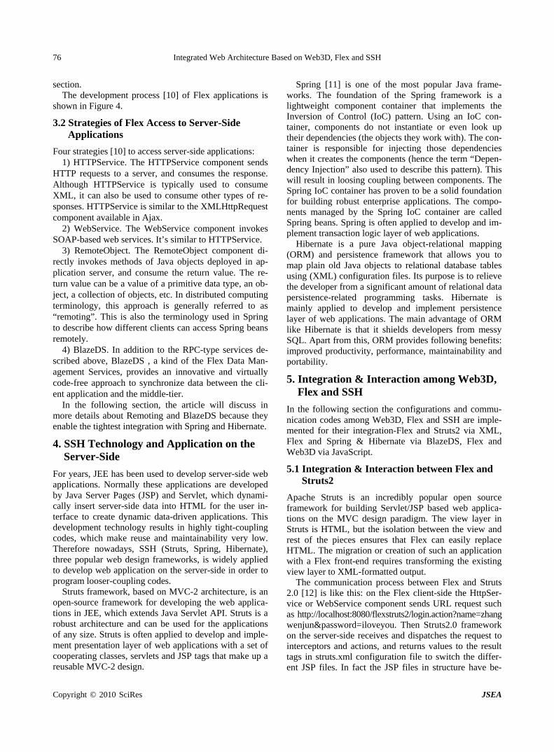
Integrated Web Architecture Based on Web3D, Flex and SSH 76
section. The development process [10] of Flex applications is
shown in Figure 4.
3.2 Strategies of Flex Access to Server-Side Applications
Four strategies [10] to access server-side applications: 1) HTTPService. The HTTPService component sends
HTTP requests to a server, and consumes the response. Although HTTPService is typically used to consume XML, it can also be used to consume other types of re-sponses. HTTPService is similar to the XMLHttpRequest component available in Ajax.
2) WebService. The WebService component invokes SOAP-based web services. It’s similar to HTTPService.
3) RemoteObject. The RemoteObject component di-rectly invokes methods of Java objects deployed in ap-plication server, and consume the return value. The re-turn value can be a value of a primitive data type, an ob-ject, a collection of objects, etc. In distributed computing terminology, this approach is generally referred to as “remoting”. This is also the terminology used in Spring to describe how different clients can access Spring beans remotely.
4) BlazeDS. In addition to the RPC-type services de-scribed above, BlazeDS , a kind of the Flex Data Man-agement Services, provides an innovative and virtually code-free approach to synchronize data between the cli-ent application and the middle-tier.
In the following section, the article will discuss in more details about Remoting and BlazeDS because they enable the tightest integration with Spring and Hibernate.
4. SSH Technology and Application on the Server-Side
For years, JEE has been used to develop server-side web applications. Normally these applications are developed by Java Server Pages (JSP) and Servlet, which dynami-cally insert server-side data into HTML for the user in-terface to create dynamic data-driven applications. This development technology results in highly tight-coupling codes, which make reuse and maintainability very low. Therefore nowadays, SSH (Struts, Spring, Hibernate), three popular web design frameworks, is widely applied to develop web application on the server-side in order to program looser-coupling codes.
Struts framework, based on MVC-2 architecture, is an open-source framework for developing the web applica-tions in JEE, which extends Java Servlet API. Struts is a robust architecture and can be used for the applications of any size. Struts is often applied to develop and imple-ment presentation layer of web applications with a set of cooperating classes, servlets and JSP tags that make up a reusable MVC-2 design.
Spring [11] is one of the most popular Java frame-works. The foundation of the Spring framework is a lightweight component container that implements the Inversion of Control (IoC) pattern. Using an IoC con-tainer, components do not instantiate or even look up their dependencies (the objects they work with). The con- tainer is responsible for injecting those dependencies when it creates the components (hence the term “Depen- dency Injection” also used to describe this pattern). This will result in loosing coupling between components. The Spring IoC container has proven to be a solid foundation for building robust enterprise applications. The compo-nents managed by the Spring IoC container are called Spring beans. Spring is often applied to develop and im-plement transaction logic layer of web applications.
Hibernate is a pure Java object-relational mapping (ORM) and persistence framework that allows you to map plain old Java objects to relational database tables using (XML) configuration files. Its purpose is to relieve the developer from a significant amount of relational data persistence-related programming tasks. Hibernate is mainly applied to develop and implement persistence layer of web applications. The main advantage of ORM like Hibernate is that it shields developers from messy SQL. Apart from this, ORM provides following benefits: improved productivity, performance, maintainability and portability.
5. Integration & Interaction among Web3D, Flex and SSH
In the following section the configurations and commu-nication codes among Web3D, Flex and SSH are imple-mented for their integration-Flex and Struts2 via XML, Flex and Spring & Hibernate via BlazeDS, Flex and Web3D via JavaScript.
5.1 Integration & Interaction between Flex and Struts2
Apache Struts is an incredibly popular open source framework for building Servlet/JSP based web applica-tions on the MVC design paradigm. The view layer in Struts is HTML, but the isolation between the view and rest of the pieces ensures that Flex can easily replace HTML. The migration or creation of such an application with a Flex front-end requires transforming the existing view layer to XML-formatted output.
The communication process between Flex and Struts 2.0 [12] is like this: on the Flex client-side the HttpSer-vice or WebService component sends URL request such as http://localhost:8080/flexstruts2/login.action?name=zhang wenjun&password=iloveyou. Then Struts2.0 framework on the server-side receives and dispatches the request to interceptors and actions, and returns values to the result tags in struts.xml configuration file to switch the differ-ent JSP files. In fact the JSP files in structure have be-
Copyright © 2010 SciRes JSEA
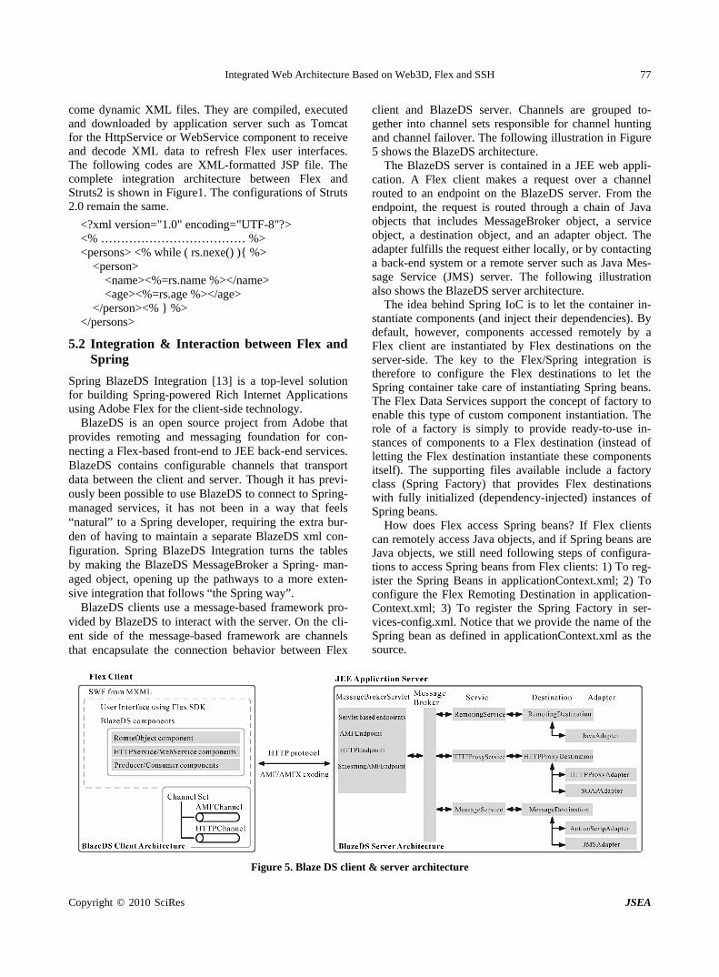
Integrated Web Architecture Based on Web3D, Flex and SSH
Copyright © 2010 SciRes JSEA
77
come dynamic XML files. They are compiled, executed and downloaded by application server such as Tomcat for the HttpService or WebService component to receive and decode XML data to refresh Flex user interfaces. The following codes are XML-formatted JSP file. The complete integration architecture between Flex and Struts2 is shown in Figure1. The configurations of Struts 2.0 remain the same.
client and BlazeDS server. Channels are grouped to-gether into channel sets responsible for channel hunting and channel failover. The following illustration in Figure 5 shows the BlazeDS architecture.
The BlazeDS server is contained in a JEE web appli-cation. A Flex client makes a request over a channel routed to an endpoint on the BlazeDS server. From the endpoint, the request is routed through a chain of Java objects that includes MessageBroker object, a service object, a destination object, and an adapter object. The adapter fulfills the request either locally, or by contacting a back-end system or a remote server such as Java Mes-sage Service (JMS) server. The following illustration also shows the BlazeDS server architecture.
<?xml version="1.0" encoding="UTF-8"?> <% ……………………………… %> <persons> <% while ( rs.nexe() ){ %>
<person> <name><%=rs.name %></name> <age><%=rs.age %></age>
The idea behind Spring IoC is to let the container in-stantiate components (and inject their dependencies). By default, however, components accessed remotely by a Flex client are instantiated by Flex destinations on the server-side. The key to the Flex/Spring integration is therefore to configure the Flex destinations to let the Spring container take care of instantiating Spring beans. The Flex Data Services support the concept of factory to enable this type of custom component instantiation. The role of a factory is simply to provide ready-to-use in-stances of components to a Flex destination (instead of letting the Flex destination instantiate these components itself). The supporting files available include a factory class (Spring Factory) that provides Flex destinations with fully initialized (dependency-injected) instances of Spring beans.
</person><% } %> </persons>
5.2 Integration & Interaction between Flex and Spring
Spring BlazeDS Integration [13] is a top-level solution for building Spring-powered Rich Internet Applications using Adobe Flex for the client-side technology.
BlazeDS is an open source project from Adobe that provides remoting and messaging foundation for con-necting a Flex-based front-end to JEE back-end services. BlazeDS contains configurable channels that transport data between the client and server. Though it has previ-ously been possible to use BlazeDS to connect to Spring- managed services, it has not been in a way that feels “natural” to a Spring developer, requiring the extra bur-den of having to maintain a separate BlazeDS xml con-figuration. Spring BlazeDS Integration turns the tables by making the BlazeDS MessageBroker a Spring- man-aged object, opening up the pathways to a more exten-sive integration that follows “the Spring way”.
How does Flex access Spring beans? If Flex clients can remotely access Java objects, and if Spring beans are Java objects, we still need following steps of configura-tions to access Spring beans from Flex clients: 1) To reg-ister the Spring Beans in applicationContext.xml; 2) To configure the Flex Remoting Destination in application-Context.xml; 3) To register the Spring Factory in ser-vices-config.xml. Notice that we provide the name of the Spring bean as defined in applicationContext.xml as the source.
BlazeDS clients use a message-based framework pro-vided by BlazeDS to interact with the server. On the cli-ent side of the message-based framework are channels that encapsulate the connection behavior between Flex
Figure 5. Blaze DS client & server architecture
Integrated Web Architecture Based on Web3D, Flex and SSH 78
5.3 Integration & Interaction between Flex and Hibernate
If Hibernate is used for web application it will be better implementing our own DataAccess objects and providing public methods of these objects to our clients by a Web-service. Hibernate persists Java objects.
Hibernate and Flex front-ends can be easily connected by using BlazeDS DataManagement Service. In Java developed classes can be accessed in the Flex application using an ActionScript class with the same setter- and getter-methods. This ActionScript class represents the Java class on the client-side. Any changes you make at the ActionScript class will be directly affecting the Java class on the server. There is no need to develop DataAc-cess classes. All create-, update-, and delete-operations are handled by DataManagement Service. Behind the scenes the class flex.data.adapters.JavaAdapter is taking care of the CRUD-Operations.
The hibernate.cfg.xml conatains common settings for the database connection, the SQL dialect and a few more which are not explained in detail here. In the my-class.hbm.xml we map the class myclass. The mapping file has a root tag called <hibernate-mapping>. Within this tag the classes are mapped for the SQL database. In more complex applications every class should have its own mapping file.
Configuration of the RMTP-Channel and the Destina-tions in Figure 5: Like all configuration files for the BlazeDS we will have the DataManagement configura-tion files in the folder [CONTEXT-ROOT]/WEB-INF/ flex of web application server, in this case the Tomcat. The important files for the application are services-config. xml and data-management-config.xml. In the services- config.xml we have to declare the RTMP Channel and the file contains this entry by default.
In the data-management-config.xml we need to declare the Destinations for our developed Java classes. In the <destination> tag we give this destination an ID which will be used later by the Flex application to refer to this particular destination.
To communicate with the Java objects at the Tomcat we need to implement ActionScript classes which are the counterpart to the Java classes—they have the same properties as the Java classes. We declare the properties public so there is no need to write getter- and setter- methods. By definition the ActionScript classes must contain an empty constructor. The classes are declared as managed and we set an alias to the corresponding Java class.
In the <mx:DataService> tag in DataService compo-nent in the Flex application, we set the property “destina-tion” to the name of the destination as we declared it in the data-management-config.xml. The DataService com- ponent also provides methods like deleteItem() and cre-
ateItem() of the typical methods of Data Access Objects. Note that we never declared or implemented these meth-ods. This work is already done by the Flex DataManage- ment Service.
5.4 Communication & Interaction between Flex and Web3D via JavaScript
In application interaction and communication between Flex and Web3D models on the client-side are required. Flex sends data to Web3D, and the Web3D models and scenes change with the received data. On the other hand, Web3D can also send data to Flex, and the visual chart-ings or tables or other components in Flex change with the received data. In addition, the Flex can forward the received data to the server-side.
How can we implement communication & interaction between Flex and Web3D? It is known that Flex runs in Flash Player, and that Web3D models and scenes run in Web3D Player. Both Flex and Web3D are embedded in HTML web pages in browser, and the direct communica-tion between Flash Player and Web3D Player is impossi-ble. However both Flex and Web3D can communicate with JavaScript in web browser, therefore JavaScript can be served as an intermediary between Flex and Web3D. That is, Flex communicates and sends data to JavaScript, then it receives and forwards the data to Web3D; on the other hand, Web3D can send data to Flex via JavaScript shown in Figure 1.
5.4.1 Calling JavaScript Functions from Flex The External Interface API is used to call JavaScript functions from Flex and build wrappers to call from Flex.
1) Flex Codes. In Flex program shown in the follow-ing example an ActionScript function is added into the Script tags, and “flash.external.*” package needs to be imported. If ExternalInterface is available, the Exter-nalInterface.call will be executed. Then the information will be sent to a JavaScript function called “displayPer-son”, whose argument is the selectedItem in a DataGrid. The status label saying “data sent” will be updated. If the ExternalInterface is not available an error message will be displayed in the label. The scripts look like this:
public function jsDisplayPerson():void{ if (ExternalInterface.available) {
ExternalInterface.call("displayPerson", dgPeople.selectedItem);
lblMessage.text = "Data Sent!";} else{lblMessage.text = "Error sending data!"; }}
2) JavaScript Codes. In HTML page the JavaScript code receives and displays the “person” sent from Flex. In a set of JavaScript tags the displayPerson function is created: note that the name has to match perfectly the ExternalInterface.call function in Flex. Firstly the Java- Script function checks whether it gets a null object, and if it is null an alert will be displayed. Then we just use the
Copyright © 2010 SciRes JSEA
Integrated Web Architecture Based on Web3D, Flex and SSH 79
object passed as a JavaScript object and reference the appropriate DataGrid columns using JavaScript object property syntax. Finally the JavaScript forwards the ob-ject to Web3D. In HTML script tags the codes can be written as below.
function displayPerson(person){ if(person = = null){
alert("Please select a person, or maybe I screwed up.");}
else{ document.getElementById('nameDisplay').innerHTML = person.Name; document.getElementById('ageDisplay').innerHTML = person.Age; document.getElementById('sexDisplay').innerHTML = person.Sex;}}
5.4.2 Calling Flex Functions from JavaScript 1) Flex Codes. To call Flex functions from JavaScript via ExternalInterface, the first step is to add some codes to the application startup to initialize Flex functions so that it is accessible through external calls.
<mx:Application xmlns:mx=http://www.adobe.com/2006/mxml initialize="initApp()">
The initApp ActionScript function checks if the Ex-ternalInterface is available and adds a callback for an ActionScript function. This function is externally re-ferred to as “addPerson” and it maps the internal function called addPerson. The initApp function is added in Ac-tionScript Script tags and shown below:
public function initApp():void{ if (ExternalInterface.available) ExternalInterface.ad
dCallback("addPerson", addPerson);}
Now the only thing left is to create the function “addPerson” in Flex, which adds persons to the DataGrid. This function takes three arguments: name, age, and sex.
public function addPerson(name:String, age:String, sex:String):void{
(dgPeople.dataProvider as ArrayCollection).addItem({Name: name, Age: age, Sex: sex});}
2) JavaScript Codes. After the MXML and Aaction-Script completed the JavaScript function grabs values from Web3D and calls the Flex function using those values as arguments. Then function getFlexApp ('Flex JSApp') is used to call the Flex function from JavaScript. The JavaScript tag is the following:
function addPerson(){ var name = document.getElementById('txtName').value; var age = document.getElementById('txtAge').value; var sex = document.getElementById('selSex').value; getFlexApp('FlexJSApp').addPerson(name, age, sex);}
This getFlexApp function in the JavaScript tag actu-ally returns the Flex application embedded in the web
page and takes into account various types of browsers. This function returns the appropriate reference, depend-ing on the browser.
function getFlexApp(appName){if (navigator.appName.indexOf ("Microsoft") !=-1){return window[appName];} else {return document[appName];}}
5.4.3 Communication between Web3D and JavaScript There are many polular Web3D technologies such as Unity3D, Flash 3D, and Google released O3D technol-ogy not long ago. In the following section we will dis-cuss O3D technology and the communication between O3D and JavaScript.
O3D [14] is an open-source JavaScript API for creat-ing interactive 3D graphics applications. O3D extends application JavaScript code with an API for 3D graphics. It uses standard JavaScript event processing and callback methods. An O3D application is contained in an HTML document. The main code for the O3D JavaScript appli-cation is contained in a <script> element inside the <head> element of the HTML document. Typically, when the HTML page is finished loading, the O3D init() function is called and executed automatically.
Because O3D is implemented by JavaScript and runs in HTML browser, it is very easy for O3D to communi-cate with Flex via JavaScript. The O3D JavaScript code of communication with Flex is very similar to the above code between Flex and JavaScript.
6. Conclusions
Several popular web frameworks, namely Web3D, Flex and Struts2-Spring-Hibernate, were studied for this in-teroperability research. The author researched how these frameworks can work together well, and created their integration architecture. Web3D was applied to simulate 3D shape and functions of products and interact with customers on the client-side; Flex was used to implement business process, rich user interfaces and data visualiza-tion on the client-side; SSH, three popular web design frameworks on the server-side, was adopted to realize transaction logic and data persistence so as to develop low-coupling codes. More importantly, the author pro-grammed their codes of integration and communication & interaction: Flex and Struts2 via XML, Flex and Spring & Hibernate via BlazeDS, Flex and Web3D via JavaScript. All research findings were applied into an application demo named “RIA & Web3D Virtual Shop-ping City”. The practice has shown that the architecture based on Web3D, Flex and SSH is effective and valu-able.
7. Acknowledgments
This research project has been sponsored by “Key Re-search Fund Project in 2009” under China Women Uni-versity.
Copyright © 2010 SciRes JSEA
Integrated Web Architecture Based on Web3D, Flex and SSH
Copyright © 2010 SciRes JSEA
80
REFERENCES
[1] W. J. Zhang, “Research of Web3D technology application in e-commerce,” in the 5th China Conference on Software Engineering, Beijing, China, Vol. 44, pp. 225–227, No-vember 2008.
[2] M. Zhang, Z. H. Lu, and X. L. Zhang, “Research and application of the 3D virtual community based on WEBVR and RIA,” Computer and Information Science, Vol. 2, No. 1, pp. 8–15, February 2009.
[3] F. Zhang and W. W. Wang, “The analyzing about Web3D virtual reality technology,” Friend of Science Amateurs, Vol. 5, pp. 130–131, May 2008.
[4] S. Chen, “Interaction design of Web3D based VR on internet,” Packaging Engineering, Vol. 29, No. 4, pp. 84–86, April 2008.
[5] D. Brutzman and L. Daly, “X3D: Extensible 3D graphics for web authors,” Elsevier Inc, 2007.
[6] J. Lott and D. Patterson, “Advanced actionscript 3 with design patterns,” Peachpit Press, 2006.
[7] Adobe Systems Incorporated, Flex 3 help, 2009. http://livedocs.adobe.com/flex/3/html/help.html?content =profiler 3.html.
[8] Adobe Systems Incorporated, Flex 3 language reference, 2009. http://livedocs.adobe.com/flex/3/langref/.
[9] Adobe Systems Incorporated, Flex 3 data visualization developer guide, 2008. http://livedocs.adobe.com/flex/3/datavis_flex3.pdf.
[10] Adobe Systems Incorporated, Flex 3 developer’s guide, 2009. http://livedocs.adobe.com/flex/3/html/help.html? content=Part2_DevApps_1.html.
[11] Walls. C, “Spring in action,” 2nd Edition, Greenwitch Manning, 2008.
[12] W. J. Zhang, “Research of RIA design pattern based on Flex, Spring and Hibernate,” in the 5th China Conference on Software Engineering, Beijing, China, Vol. 44, pp. 126–128, November 2008.
[13] J. Grelle, “Spring BlazeDS integration reference guide,” March, 2009. http://static.springframework.org/spring-flex/docs/1.0.x/reference/html/index.html.
[14] Google, O3D developer’s guide, 2009. http://code.google.com/intl/zh-CN/apis/o3d/docs/devguideintro.html.
J. Software Engineering & Applications, 2010, 3: 81-90 doi:10.4236/jsea.2010.31010 Published Online January 2010 (http://www.SciRP.org/journal/jsea)
Copyright © 2010 SciRes JSEA
Analysis and Comparison of Five Kinds of Typical Device-Level Embedded Operating Systems
Jialiang WANG, Hai ZHAO, Peng LI, Hui LI, Bo LI
School of Information Science and Engineering, Northeastern University, Shenyang, China. Email: [email protected] Received September 1st, 2009; revised September 21st, 2009; accepted September 27th, 2009.
ABSTRACT
Today, the number of embedded system was applied in the field of automation and control has far exceeded a variety of general-purpose computer. Embedded system is gradually penetrated into all fields of human society, and ubiquitous embedded applications constitute the "ubiquitous" computing era. Embedded operating system is the core of the em-bedded system, and it directly affects the performance of the whole system. Our Liaoning Provincial Key Laboratory of Embedded Technology has successfully developed five kinds of device-level embedded operating systems by more than ten years’ efforts, and these systems are Webit 5.0, Worix, μKernel, iDCX 128 and μc/os-II 128. This paper mainly analyses and compares the implementation mechanism and performance of these five kinds of device-level embedded operating systems in detail. Keywords: Embedded System, Operating System Core, Real-Time Ability, I/O Delay and Jitter, Pervasive Computing and Internet of Things
1. Introduction
Embedded system has played a significant role in the field of industrial manufacture, process control, instru-mentation, consumer electronics and military devices and so on. Embedded operating system has a wide range of space not only in the traditional industrial control and business applications, but also in the field of information household electrical appliances, which has brought much convenience to us [1,2].
The using scope of industrial automation devices based on embedded singlechip has been greatly expanded in recent years. The network is the mainly method not only to improve production efficiency and product qual-ity but also to reduce the cost of human resources, such as the application of industrial control, digital machine tool, grid power system, security power system, device inspection, system monitoring and petrochemicals and so on. Embedded system originated in the age of micro-computer, however the size, price and reliability of a microcomputer are unable to meet the need of majority of embedded system applications. Therefore, embedded system must follow the way of independent development, and this way is just the way of the singlechip. Singlechip has enhanced the fast improvement of embedded tech-nology. Among the field of almost traditional process control, 8-bit singlechip is widely used, but the device
-level embedded operating systems can be used for them are very few. So the developing of device-level embed-ded operating system is very necessary.
2. Embedded Operating System
Embedded operating system is mainly used to monitor and control devices, and general desktop operating sys-tem is largely based on the orders of keyboard and mouse. Relatively speaking, the movement of device has very strict timing requirements, but the timing of human ac-tion and reflection are not so strict. So for many applica-tion fields of device-level control environment, the gen-eral desktop operating system is not well competent. Comparing to the micro-computers and large-scale gen-eral-purpose computer operating systems, the embedded operating system has the basic features of real-time per-formance, small core code, preemptive kernel, being configured, reduction and high reliability and so on.
The technology of EI (Embedded Internet) makes it possible of a large number of traditional devices and home electrical appliances instruments achieving net-work interconnection. It has become a trend for RTOS (real-time operating system) is used in EI applications, and it mainly due to the RTOS not only improves the reliability of the system, but also it can reduce the diffi-cult of development of embedded software and improve
Analysis and Comparison of Five Kinds of Typical Device-Level Embedded Operating Systems 82
development efficiency. Different from general embed-ded applications, EI applications require RTOS not only has good real-time kernel, but also can provide the capa-bilities of network protocol stack and certain document management. For most of the existing commercial and free RTOS, they are either very expensive or not having network protocol stack modules, especially for the 8-bit microcontroller with a network of RTOS functions are very few.
Our Liaoning Provincial Key Laboratory of Embedded Technology has successfully developed five kinds de-vice- level embedded operating systems running on 8-bit singlechip, and these systems are Webit 5.0, Worix, μKernel, iDCX 128 and μc/os-II 128. The experimental platform used to develop and test is ATmega 128L manufactured by the United States ATMEL corporation. ATmega 128L is one of the most powerful singlechip in the series of AVR, and AVR singlechip is the first gen-eral RISC architecture singlechip, so its process speed and performance has greatly improved than the MCS-51 series singlechip of CISC architecture.
3. Introduction of Five Kinds of Typical Device-Level Embedded Operating System
3.1 Webit 5.0 Embedded Operating System
Webit is an embedded internet device, which has been successfully embedded into the fieldbus devices and can successfully access to devices through the internet. Webit takes full advantage of singlechip system’s limited re-sources, and combined with TCP/IP protocol and high- performance network to process data. Webit has been successfully developed and manufactured by our Liaon-ing Provincial Key Laboratory of Embedded Technology, and it has passed the appraisal of national science and technology department, and it has also achieved the new product patent of state intellectual property office.
Webit 5.0 operating system directly runs on the device driver, and it mainly achieves the functions of task man-agement, synchronization and communication between tasks. The modules of network file system, protocol stack and I/O management are running outside of system core. The design of task scheduling strategy of Webit 5.0 sys-tem adopting the multi-tasking kernel based on priority scheduling, thus the time performance of the kernel is better, and it makes the tasks with high real-time ability can well gain the system resources and have the ability of quick response. The system uses the mechanisms of mailbox and semaphores to achieve synchronization and communication for inter-task, while it also provides ef-fective mechanism of network authentication and user rights so as to ensure the safety of the system. Webit 5.0 is developed in accordance with the method of modular design, using the micro-kernel technology. TCP/IP pro-tocol suite, I/O interface and user interface are separated
from the kernel, so it results in the architecture of hierar-chy. Each layer corresponds to a module respectively, and each module is separated designed. The call between modules is given interface specification, so it can realize the purposes of flexible reduction based on user demands, and the system is well applied in the field of industrial control.
3.2 WORIX Embedded Operating System
WORIX operating system has the following features: 1) System can accomplish a variety of concurrent op-
erations through multi-task. If the user's application re-quires more additional tasks, they can modify the con-stant value of kernel THREAD_NUMS to reset the max- imum number of tasks that the system supports;
2) Scheduling algorithm of the system is based on static priority preemptive scheduling, so that system can ensure that high-priority task can have the ability of fast response;
3) The system can support different network protocol stack, and users can develop their own network protocols by wireless modules driver interface supported by the operating system, so it can be well applied in the field of wireless sensor networks;
4) WORIX kernel implements the mechanism of semaphores and mutual semaphores so as to let the task to access to exclusive resources;
5) The clock beat of WORIX kernel was set by the in-ternal timer /counter Timer 0. The timer runs interrupt service program every time interval, thus sleep task and wake-up function were handled in the timer interrupt service.
3.3 μKernel Embedded Operating System
The core of the μKernel operating system retains the most basic and important system services, which includ-ing the functions of task management, task scheduling, mutual exclusion semaphores and clock management. Other specific system function modules can be selected in the application part so as to minimize the kernel code size. Time management mechanism is designed as fol-lows: set the time of delay with the unit of clock beat, when the system delays a task for some time, it gets the task from the task ready table, and puts it into the waiting list. This mechanism allows the task can be delayed for a number of clock beat, and it also provides the basis to judge whether waiting tasks exceed their timeout. The design of semaphore aims at establishing a sign of whether the shared resource is occupied. Thus while ac-cessing to shared resource; task may check the sign to know whether the shared resource is occupied. The processing of shared data uses semaphores doesn’t in-creasing the amount of interrupt delay time. If the inter-rupt service program or the current task activates a high-priority task, the high-priority task will be immedi-
Copyright © 2010 SciRes JSEA
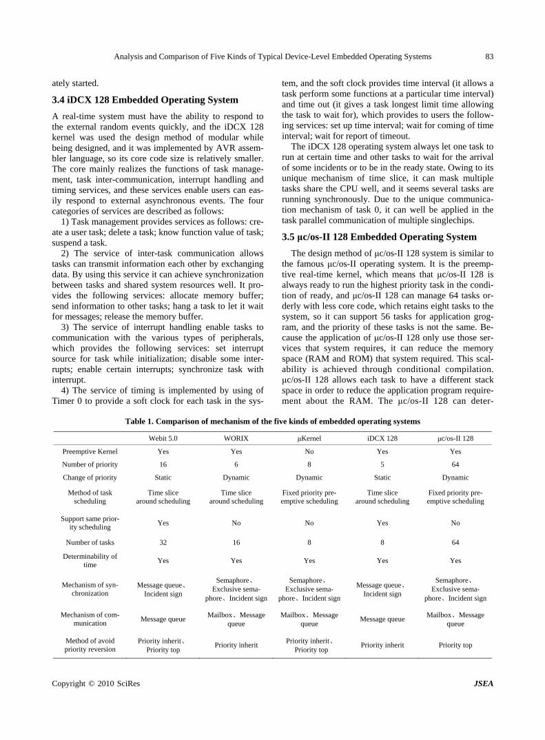
Analysis and Comparison of Five Kinds of Typical Device-Level Embedded Operating Systems
Copyright © 2010 SciRes JSEA
83
ately started.
3.4 iDCX 128 Embedded Operating System
A real-time system must have the ability to respond to the external random events quickly, and the iDCX 128 kernel was used the design method of modular while being designed, and it was implemented by AVR assem-bler language, so its core code size is relatively smaller. The core mainly realizes the functions of task manage-ment, task inter-communication, interrupt handling and timing services, and these services enable users can eas-ily respond to external asynchronous events. The four categories of services are described as follows:
1) Task management provides services as follows: cre-ate a user task; delete a task; know function value of task; suspend a task.
2) The service of inter-task communication allows tasks can transmit information each other by exchanging data. By using this service it can achieve synchronization between tasks and shared system resources well. It pro-vides the following services: allocate memory buffer; send information to other tasks; hang a task to let it wait for messages; release the memory buffer.
3) The service of interrupt handling enable tasks to communication with the various types of peripherals, which provides the following services: set interrupt source for task while initialization; disable some inter-rupts; enable certain interrupts; synchronize task with interrupt.
4) The service of timing is implemented by using of Timer 0 to provide a soft clock for each task in the sys-
tem, and the soft clock provides time interval (it allows a task perform some functions at a particular time interval) and time out (it gives a task longest limit time allowing the task to wait for), which provides to users the follow-ing services: set up time interval; wait for coming of time interval; wait for report of timeout.
The iDCX 128 operating system always let one task to run at certain time and other tasks to wait for the arrival of some incidents or to be in the ready state. Owing to its unique mechanism of time slice, it can mask multiple tasks share the CPU well, and it seems several tasks are running synchronously. Due to the unique communica-tion mechanism of task 0, it can well be applied in the task parallel communication of multiple singlechips.
3.5 μc/os-II 128 Embedded Operating System
The design method of μc/os-II 128 system is similar to the famous μc/os-II operating system. It is the preemp-tive real-time kernel, which means that μc/os-II 128 is always ready to run the highest priority task in the condi-tion of ready, and μc/os-II 128 can manage 64 tasks or-derly with less core code, which retains eight tasks to the system, so it can support 56 tasks for application grog-ram, and the priority of these tasks is not the same. Be-cause the application of μc/os-II 128 only use those ser-vices that system requires, it can reduce the memory space (RAM and ROM) that system required. This scal-ability is achieved through conditional compilation. μc/os-II 128 allows each task to have a different stack space in order to reduce the application program require- ment about the RAM. The μc/os-II 128 can deter-
Table 1. Comparison of mechanism of the five kinds of embedded operating systems
Webit 5.0 WORIX μKernel iDCX 128 μc/os-II 128
Preemptive Kernel Yes Yes No Yes Yes
Number of priority 16 6 8 5 64
Change of priority Static Dynamic Dynamic Static Dynamic
Method of task scheduling
Time slice around scheduling
Time slice around scheduling
Fixed priority pre-emptive scheduling
Time slice around scheduling
Fixed priority pre-emptive scheduling
Support same prior-ity scheduling
Yes No No Yes No
Number of tasks 32 16 8 8 64
Determinability of time
Yes Yes Yes Yes Yes
Mechanism of syn-chronization
Message queue、 Incident sign
Semaphore、Exclusive sema-
phore、Incident sign
Semaphore、Exclusive sema-
phore、Incident sign
Message queue、 Incident sign
Semaphore、Exclusive sema-
phore、Incident sign
Mechanism of com-munication
Message queue Mailbox、Message
queue Mailbox、Message
queue Message queue
Mailbox、Message queue
Method of avoid priority reversion
Priority inherit、Priority top
Priority inherit Priority inherit、
Priority top Priority inherit Priority top
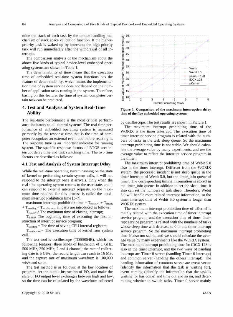
Analysis and Comparison of Five Kinds of Typical Device-Level Embedded Operating Systems 84
mine the stack of each task by the unique handling me- chanism of stack space validation function. If the higher- priority task is waked up by interrupt; the high-priority task will run immediately after the withdrawal of all in-terrupts.
The comparison analysis of the mechanism about the above five kinds of typical device-level embedded oper-ating systems are shown in Table 1.
The determinability of time means that the execution time of embedded real-time system functions has the feature of determinability, which means the implementa-tion time of system service does not depend on the num-ber of application tasks running in the system. Therefore, basing on this feature, the time of system completes cer-tain task can be predicted.
4. Test and Analysis of System Real-Time Ability
The real-time performance is the most critical perform-ance indicators to all control systems. The real-time per-formance of embedded operating system is measured primarily by the response time that is the time of com-puter recognizes an external event and before reacting it. The response time is an important indicator for running system. The specific response factors of RTOS are: in-terrupt delay time and task switching time. The two time factors are described as follows:
4.1 Test and Analysis of System Interrupt Delay
While the real-time operating system running on the state of kernel or performing certain system calls, it will not respond to the interrupt once it arrivals. Only when the real-time operating system returns to the user state, and it can respond to external interrupt requests, so the maxi-mum time required for this process is called the maxi-mum interrupt prohibition time [3–7].
maximum interrupt prohibition time = TcloseINT + TdoISR
+ TsaveReg + TstartService, all parts are introduced as follows:
TcloseINT: The maximum time of closing interrupt;
TdoISR: The beginning time of executing the first in-struction of interrupt service program;
TsaveReg = The time of saving CPU internal registers; TstartService = The execution time of kernel runs system
call. The test tool is oscilloscope (TDS5054B), which has
following features: three kinds of bandwidth of 1 GHz, 500 MHz, 350 MHz; 2 and 4 channel; the rate of collect-ing date is 5 GS/s; the record length can reach to 16 MS, and the capture rate of maximum waveform is 100,000 wfs/s and so on.
The test method is as follows: at the key location of program, set the output instruction of I/O, and make the state of I/O output level exchanges between high and low, so the time can be calculated by the waveform collected
1 2 3 4 5 6 7 810
15
20
25
30
35
40
45
50
55
60
Number of running tasks
Te
st v
alu
e o
f ma
xim
um
inte
rru
pt p
roh
ibiti
on
tim
e (μ
s)
WorixWebit 5.0μc/os- 128Ⅱ
iDCX 128μKernel
Figure 1. Comparison of the maximum interruption delay time of the five embedded operating systems by oscilloscope. The test results are shown in Picture 1.
The maximum interrupt prohibiting time of the WORIX is the timer interrupt. The execution time of timer interrupt service program is related with the num-bers of tasks in the task sleep queue. So the maximum interrupt prohibiting time is not stable. We should calcu-late the average value by many experiments, and use the average value to reflect the interrupt service program in the timer.
The maximum interrupt prohibiting time of Webit 5.0 also in the timer interrupt. Different from the WORIX system, the processed incident is not sleep queue in the timer interrupt of Webit 5.0, but the timer_info queue of timer. The corresponding timing information is stored in the timer_info queue. In addition to set the sleep time, it also can set the numbers of task sleep. Therefore, Webit 5.0 will handle more related interrupt information, so the timer interrupt time of Webit 5.0 system is longer than WORIX system.
The maximum interrupt prohibition time of μKernel is mainly related with the execution time of timer interrupt service program, and the execution time of timer inter-rupt service program is related with the numbers of tasks whose sleep time will decrease to 0 in this timer interrupt service program. So the maximum interrupt prohibiting time is also not stable, and we should calculate the aver-age value by many experiments like the WORIX system. The maximum interrupt prohibiting time for iDCX 128 is also in the timer interrupt, and the two ways of handing interrupt are Timer 0 server (handling Timer 0 interrupt) and common server (handing the others interrupt). The handing information of common server are event vector (identify the information that the task is waiting for), event coming (identify the information that the task is waiting for has come) and time out and so on, and deter-mining whether to switch tasks. Timer 0 server mainly
Copyright © 2010 SciRes JSEA
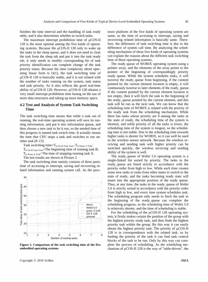
Analysis and Comparison of Five Kinds of Typical Device-Level Embedded Operating Systems 85
finishes the time interval and the handling of task ready table, and it also determines whether to switch tasks.
The maximum interrupt prohibition time of μCOS-II 128 is the most optimal among the five kinds of operat-ing systems. Because the μCOS-II 128 only to wake up the tasks in the sleep queue, and it does not need to clear the task from the sleep tab and put it into the task ready tab, it only needs to modify corresponding bit of task priority identification can complete change of the task priority status. Because the time complexity about oper-ating linear form is O(1), the task switching time of μCOS-II 128 is basically stable, and it is not related with the number of tasks running on the system, task status and task priority. So it also reflects the good real-time ability of μCOS-II 128. However, μCOS-II 128 obtains a very small interrupt prohibition time basing on the use of more data structures and taking up more memory space.
4.2 Test and Analysis of System Task Switching Time
The task switching time means that while a task out of running, the real-time operating system will save its run-ning information, and put it into information queue, and then choose a new task to let it run, so the needed time of this progress is named task switch time. It actually means the time that CPU stops a task and switches to run an-other task [8–13].
Task switching time=Tto Do B Task Time–Tto Pause A Task: Tto Do B Task Time=The beginning time of running task B; Tto Pause A Task=The time of stopping running task A. The test results are shown in Picture 2. The task switching time mainly consists of three parts:
time of accessing to interrupt, saving and recovering re-lated information and running system call. As the proc-
1 2 3 4 5 6 7 815
20
25
30
35
40
45
Number of running tasks
Te
st v
alu
e o
f ta
sk s
witc
hin
g ti
me
(μ
s)
WorixWebit 5.0μc/os- 128ⅡiDCX 128μKernel
Figure 2. Comparison of the task switching time of the five embedded operating systems
essor platform of the five kinds of operating system are same, so the time of accessing to interrupt, saving and recovering related information is basically same. There-fore, the difference of task switching time is due to the difference of system call time. By analyzing the sched-uling mechanism of these five kinds of operating systems can explain the reasons about the different task switching time of these operating systems.
The ready queue of WORIX operating system using a pointer array, and the elements of the array points to the pointer of the beginning of correspondingly priority ready queue. While the system schedules tasks, it will traverse the ready_queue from beginning, if the content pointed by the current element location is empty, it will continuously traverse to later elements of the ready_queue; if the content pointed by the current element location is not empty, then it will fetch the task in the beginning of the ready_queue pointed by the current element, and this task will be run as the next task. We can know that the scheduling time of WORIX is related with the priority of the ready task from the scheduling mechanism. While there has tasks whose priority are 0 among the tasks in the state of ready, the scheduling time of the system is shortest; and while priority of all the tasks is lower, the scheduling time of the system is longest, so the schedul-ing time is not stable. Due to the scheduling time towards higher tasks is shorter for WORIX, so it can well be used in the wireless sensor network. Because the wireless re-ceiving and sending task with higher priority can be switched quickly, the wireless receiving and sending ability of the system is well.
The ready_queue of Webit 5.0 operating system is a single-linked list sorted by priority. The tasks in the ready_queue are listed strictly in accordance with the priority order from high to low. While each time creates some new tasks or tasks from other states to switch to the state of ready, and the tasks becoming ready state will insert into the appropriate position of the ready queue. Thus, at any time, the tasks in the ready_queue of Webit 5.0 is strictly sorted in accordance with the priority order from high to low, and every time system schedules task. The scheduling program only needs to fetch the task in the beginning of the ready_queue can complete the scheduling progress, so the scheduling time of Webit 5.0 is relatively shorter, and the time of scheduling is stable.
For the scheduling of the μCOS-II 128 operating sys-tem, it firstly makes certain the position of the group with the highest priority ready task, and then finds the highest priority task within the group. By this way it can easily obtain the highest priority task. The priority of μCOS-II 128 is in correspondence with the related task, so by finding the priority of the task it can find task control blocks of the task to be run. Only by this way can com-plete the process of scheduling. As the scheduling me- chanism of μCOS-II 128 is the way of "table-driven", the
Copyright © 2010 SciRes JSEA
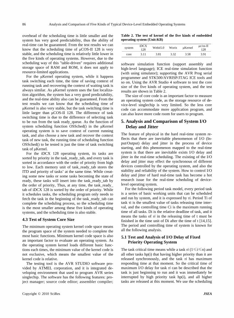
Analysis and Comparison of Five Kinds of Typical Device-Level Embedded Operating Systems 86
overhead of the scheduling time is little smaller and the system has very good predictability, thus the ability of real-time can be guaranteed. From the test results we can know that the scheduling time of μCOS-II 128 is very stable, and the scheduling time is relatively little lower in the five kinds of operating systems. However, due to the scheduling way of this "table-driven" requires additional storage space of RAM and ROM, it does not apply to resource-limited applications.
For the μKernel operating system, while it happens task switching each time, the time of saving context of running task and recovering the context of waiting task is always similar. As μKernel system uses the fast localiza-tion algorithm, the system has a very good predictability, and the real-time ability also can be guaranteed. From the test results we can know that the scheduling time of μKernel is also very stable, but the task switching time is little larger than μCOS-II 128. The difference of task switching time is due to the difference of selecting task to be run from the task ready_queue. As the function of system scheduling function OSSched() in the μKernel operating system is to save context of current running task, and also choose a new task and recover the context task of new task, the running time of scheduling function OSSched() to be tested is just the time of task switching task of μKernel.
For the iDCX 128 operating system, its tasks are sorted by priority in the task_ready_tab, and every task is sorted in accordance with the order of priority from high to low. Each memory unit of task_ready_tab stores the ITD and priority of tasks’ at the same time. While creat-ing some new tasks or some tasks becoming the state of ready, these tasks will insert into the task_ready_tab by the order of priority, Thus, at any time, the task_ready_ tab of iDCX 128 is sorted by the order of priority. While it schedules tasks, the scheduling program only needs to fetch the task in the beginning of the task_ready_tab can complete the scheduling process, so the scheduling time is the most smaller among these five kinds of operating systems, and the scheduling time is also stable.
4.3 Test of System Core Size
The minimum operating system kernel code space means the program space of the system needed to complete the most basic functions. Minimum kernel code space is also an important factor to evaluate an operating system. As the operating system kernel loads different basic func-tions each times, the minimum value of the kernel code is not exclusive, which means the smallest value of the kernel code is relative.
The testing tool is the AVR STUDIO software pro-vided by ATMEL corporation, and it is integrated de-veloping environment that used to program AVR series singlechip. The software has the following features: pro-ject manager; source code editor; assembler compiler;
Table 2. The test of kernel of the five kinds of embedded operating system (Unit:KB)
systemiDCX 128
Webit5.0 Worix μKernel μc/os-II
128
core 3.11 3.81 3.32 3.58 3.91
software simulation function (support assembly and high-level language); ICE real-time simulation function (with using simulator); supporting the AVR Prog serial programmer and STK500/AVRISP/JTAG ICE tools and so on. Using the AVR Studio 4 software to test the core size of the five kinds of operating system, and the test results are shown in Table 2.
The size of core code is an important factor to measure an operating system code, as the storage resource of de-vice-level singlechip is very limited. So the less core code can accommodate more application program, and can also leave more code room for users to program.
5. Analysis and Comparison of System I/O Delay and Jitter
The feature of physical in the hard real-time system re-flects that there are inevitable phenomenon of I/O (In-put/Output) delay and jitter in the process of device starting, and this phenomenon mapped to the real-time system is that there are inevitable exists I/O delay and jitter in the real-time scheduling. The existing of the I/O delay and jitter may effect the synchronous of different devices controlled by the operating system, and also the stability and reliability of the system. How to control I/O delay and jitter of hard real-time task has become a hot research issue for the real-time scheduling of device- level operating system.
For the following period task model, every period task is a series of basic working units that can be scheduled and run by system, and it is expressed by τi. Period Ti of task τi is the smallest value of tasks releasing time inter-val, and the controlling time Ci is the maximum running time of all tasks. Di is the relative deadline of task, and it means the tasks of τi in the releasing time of t must be finished in the time unit of Di after the time of t [14,15]. The period and controlling time of system is known for all the following analysis.
5.1 Test and Analysis of I/O Delay of Fixed Priority Operating System
The task critical time means while a task τi (1≤i≤n) and all other tasks hp(i) that having higher priority than it are released synchronously, and the task τi has maximum responding time at that moment. So the critical time of maximum I/O delay for task τi can be described that the task is just beginning to run and it was immediately be interrupted by high priority task hp(i), and all higher tasks are released at this moment. We use the scheduling
Copyright © 2010 SciRes JSEA

Analysis and Comparison of Five Kinds of Typical Device-Level Embedded Operating Systems
Copyright © 2010 SciRes JSEA
87
Li(b)pree is the maximum solution that meets (4), and it
can be calculated with the original value of Li(b)pree(0)=Ti
by iterative calculation.
method with preemptive threshold value, and allow a time threshold value, and calculate it by the preemptive and not preemptive parts respectively.
The maximum I/O delay of preemptive part of task τi is:
The minimum I/O delay of not preemptive part of task τi is:
( )
pp ii i
k hp i k
LL TH C
T
k
i
(1)
Lip is the least solution that meets (1),it can be calcu-
lated with the original value of Lip (0) = THi by iterative
calculation. The maximum I/O delay of not preemptive part of task
τi is: npi iL C TH (2)
So the maximum I/O delay of task τi based on fixed priority scheduling is:
( )
max p npi i i
pi
i kk hp i k
L L L
LC C
T
(3)
hp(i) is the task set whose priority is higher than the task τi, and Li
max is the least solution that meets (3), and it can be calculated with the original value of Li
max (0)=Ci by iterative calculation.
5.2 Test and Analysis of I/O Jitter of Fixed Priority Operating System
The minimum I/O delay is the least responding time for fixed priority scheduling, so the minimum I/O delay of preemptive part of task τi (1≤i≤n) is:
( )( )
( )
min( , )b p
b p b bi ki i i
k hp i k
L TL C TH
T
kC
i
i
(4)
( ) max( , )b np bi i iL C TH TH (5)
So the minimum I/O delay of the task τi based on the fixed priority scheduling is:
( ) ( ) ( ) max( , )min b p b np b p bi i i i i iL L L L C TH TH (6)
The maximum I/O jitter of not preemptive task τi
based on the fixed priority scheduling can be calculated by the combination of (3) and (6):
max max mini i iJ L L (7)
The operating system of iDCX 128 and Webit 5.0 are both based on fixed priority, testing the I/O delay and jitter while there are 7 tasks running on the system, and the test results are shown in Figure 3.
As we can see from the Figure 3, the Webit 5.0 oper-ating system can well optimize the I/O jitter than iDCX 128 operating system under the condition of the system can be scheduled. But with the increasing of system pay-load, the optimized effect of Webit 5.0 is decreasing con-tinuously, and the cost of this strategy is that the average I/O delay time of Webit 5.0 is much larger than iDCX 128 while system payload exceeds 0.4.
5.3 Test and Analysis of I/O Delay of Dynamic Priority Operating System
Allocate preemptive time threshold THi (0≤THi≤Ci) for task τi (1≤i≤n), and the value of I/O delay created by EDF scheduling needed to be calculated by the preemptive and not preemptive part respectively.
The maximum I/O delay of preemptive of task τi is:
0.1 0.2 0.3 0.4 0.5 0.6 0.7 0.80
5
10
15
20
25
30
35
Payload
Tes
t va
lue
of I
/O d
elay
(μ
s) Webit 5.0
iDCX 128
0.1 0.2 0.3 0.4 0.5 0.6 0.7 0.80
1
2
3
4
5
6
7
Payload
Tes
t va
lue
of I
/O ji
tter
Webit 5.0
iDCX 128
Figure 3. The test of I/O delay and jitter of iDCX 128 and Webit 5.0
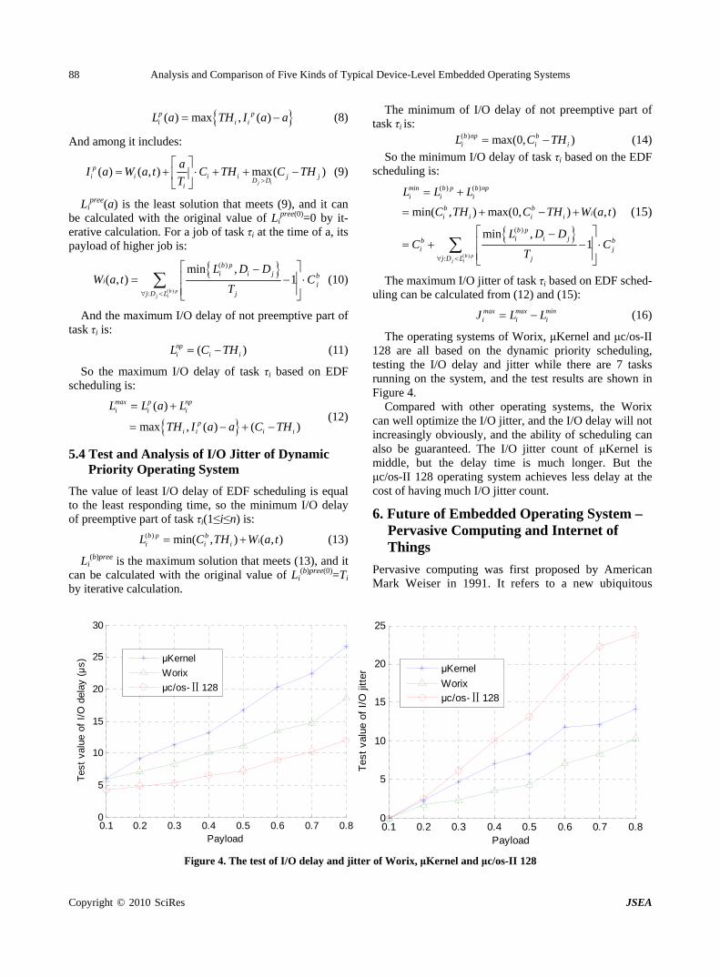
Analysis and Comparison of Five Kinds of Typical Device-Level Embedded Operating Systems 88
( ) max , ( )p pi i iL a TH I a a (8)
And among it includes:
( ) ( , ) max( )j i
pi i i i j
D Di
ajI a W a t C TH C TH
T
(9)
Lipree(a) is the least solution that meets (9), and it can
be calculated with the original value of Lipree(0)=0 by it-
erative calculation. For a job of task τi at the time of a, its payload of higher job is:
( )
( )
:
min ,( , ) 1
b pj i
b pi i j b
i jj D L j
L D DW a t C
T
)i
a t
iTH
(10)
And the maximum I/O delay of not preemptive part of task τi is:
(npi iL C TH (11)
So the maximum I/O delay of task τi based on EDF scheduling is:
( )
max , ( ) ( )
max p npi i i
pi i i i
L L a L
TH I a a C TH
(12)
5.4 Test and Analysis of I/O Jitter of Dynamic Priority Operating System
The value of least I/O delay of EDF scheduling is equal to the least responding time, so the minimum I/O delay of preemptive part of task τi(1≤i≤n) is:
( ) min( , ) ( , )b p bii i iL C TH W (13)
Li(b)pree is the maximum solution that meets (13), and it
can be calculated with the original value of Li(b)pree(0)=Ti
by iterative calculation.
The minimum of I/O delay of not preemptive part of task τi is:
( ) max(0, )b np bi iL C (14)
So the minimum I/O delay of task τi based on the EDF scheduling is:
( )
( ) ( )
( )
:
min( , ) max(0, ) ( , )
min ,1
b pj i
min b p b npi i i
b bii i i i
b pi i jb b
i jj D L j
L L L
C TH C TH W a t
L D DC C
T
(15)
The maximum I/O jitter of task τi based on EDF sched-uling can be calculated from (12) and (15):
max max mini i iJ L L (16)
The operating systems of Worix, μKernel and μc/os-II 128 are all based on the dynamic priority scheduling, testing the I/O delay and jitter while there are 7 tasks running on the system, and the test results are shown in Figure 4.
Compared with other operating systems, the Worix can well optimize the I/O jitter, and the I/O delay will not increasingly obviously, and the ability of scheduling can also be guaranteed. The I/O jitter count of μKernel is middle, but the delay time is much longer. But the μc/os-II 128 operating system achieves less delay at the cost of having much I/O jitter count.
6. Future of Embedded Operating System – Pervasive Computing and Internet of Things
Pervasive computing was first proposed by American Mark Weiser in 1991. It refers to a new ubiquitous
0.1 0.2 0.3 0.4 0.5 0.6 0.7 0.80
5
10
15
20
25
30
Payload
Tes
t va
lue
of I
/O d
elay
(μ
s)
μKernel
Worix
μc/os- 128Ⅱ
0.1 0.2 0.3 0.4 0.5 0.6 0.7 0.80
5
10
15
20
25
Payload
Tes
t va
lue
of I
/O ji
tter
μKernel
Worixμc/os- 128Ⅱ
Figure 4. The test of I/O delay and jitter of Worix, μKernel and μc/os-II 128
Copyright © 2010 SciRes JSEA
Analysis and Comparison of Five Kinds of Typical Device-Level Embedded Operating Systems 89
method of computing can be applied to various informa-tion devices. In the era of pervasive computing, comput-ing devices and the computing environment emerges together closely, and people can access to information and processing at any time and any place, and they will not fell the process of computing at all while using it. It was also considered as the next generation computing model, and the ubiquitous computing devices used are mobile computing devices mostly. Mobile computing devices are essentially part of embedded devices, so it can be said that ubiquitous computing constitutes the indispensable operating platform of the embedded sys-tem. The rapid development of embedded systems is also a strong impetus to the fast development of pervasive computing. While all physical objects of real world are linked by the internet and can be managed intelligently, it means the age of Internet of Things is coming, and peo-ple can access to appliances information easily through the internet, but this process is inseparable from the large support of operating system. So the device-level embed-ded operating system is the indispensable key technology to the coming of Internet of Things.
7. Conclusions
Embedded operating system with stable performance has played a very crucial role to the normal operation of de-vices. So the embedded operating system is considered as the cornerstone in the field of device control. This paper describes the features and implementation mechanisms of the five typical device-level embedded operating sys-tems that are independently developed by our laboratory, and also tests and analyzes the real-time performance, I/O delay and jitter. The five kinds of operating systems has well applied in the fields of Chunlanjing air-condi-tioning, Taiwan Guanyu uninterruptible power supply, network intelligent devices, and monitoring devices and so on. As the five kinds of operating system cores all have good portability and performance by long-term us-ing, and the most important is that they have the advan-tages that they can be easily operated in other device- level singlechip platforms in the fields of automation and device control, etc. So it brought broad application pros-pects for users to choose device-level embedded operat-ing systems.
8. Acknowledgments
This work is supported by the Cultivation Fund of the Key Scientific and Technical Innovation Project, Minis-try of Education of China (NO708026).
REFERENCES [1] H. Zhao, “Embedded Internet [M],” Beijing: Tsinghua
University Press, pp. 27–40, 2002.
[2] F. Robert, “Embedded Internet systems come home [J],” IEEE Internet Computing, Vol. 40, No. 14, pp. 52–53, 2001.
[3] Jacek W. “Embedded Internet technology in process con-trol devices [J],” IEEE Internet Computing, Vol. 34, No. 3, pp. 301–308, 2000.
[4] R. Bergamaschi, S. Bhattacharya, and R. Wagner, “Auto-mating the design of SoCs using cores [J],” IEEE Design &Test of Computers, , Vol. 18, No. 5, pp. 32–45, 2001.
[5] A. Garcey, and V. Lessey, “Design to time real-time scheduling [J],” IEEE Transcations on Systems, Man and Cybernetics, Vol. 23, No. 6, pp. 58–67, 1993.
[6] M. Hiroyuki, and E. Thomas, “An improved randomized on-line algorithm for a weighted interval selection prob-lem [J],” Journal of Scheduling, Vol. 7, No. 4, pp. 293–311, 2004.
[7] D. L. Liu, X. B. S. Hu, D. L. Michael, et al. “Firm real-time system scheduling based on a novel QoS con-straint [J],” IEEE Transactions on Computers, Vol. 55, No. 3, pp. 320–333, 2006.
[8] J. P. S L. Lehoczky, “Performance of real-time bus sched-uling algorithms [J],” ACM Performance Evaluation Re-view, Vol. 14, No. 1, pp. 44–53, 1986.
[9] E. Tavares, P. Maciel, and B. Silva, “Modeling hard real-time systems considering inter-task relations, dy-namic voltage scaling and overheads [J],” Microproces-sors& Microsystems, Vol. 32, No. 8, pp. 460–473, 2008.
[10] Y. Zou, M. Li, and Q. Wang, “Analysis for scheduling theory and approach of open real-time system [J],” Jour-nal of Software, Vol. 14, No. 1, pp. 83–90, 2003.
[11] C. L. Liu, and J. W. Layland, “Scheduling algorithms for multiprogramming in a hard-real-time environment [J],” Journal of the ACM. Vol. 20, No. 1, pp. 46–61, 1973.
[12] M. Sabeghi, P. Deldari, and S. Khajouei, “A fuzzy algo-rithm for scheduling periodic tasks on multiprocessor soft real-time systems [C],” Proceedings of the 17th IASTED international conference on modelling and simulation, May, Montreal, Canada, pp. 436–442, 2006.
[13] D. Liu, W. Y. Xing, R. Li, C. Y. Zhang, et al. “A fault-tolerant real-time scheduling algorithm in software fault-tolerant module [C],” Proceedings of the 7th inter-national conference on Computational Science, Part IV. Beijing, China, pp. 961–964, May, 2007.
[14] D. D. Luo, “Optimizing scheduling for hard real- time tasks in embedded systems [D],” Shenyang: Northeastern University, 2008.
[15] M. Caccamo, G. Buttazzo, and D. C. Thomas, “Efficient reclaiming in reservation-based real-time systems with variable execution times [J],” IEEE Transactions on Com-puters, No. 2, pp. 198–213, 2005.
Copyright © 2010 SciRes JSEA

Analysis and Comparison of Five Kinds of Typical Device-Level Embedded Operating Systems 90
Research Background
The appearance of embedded internet technology enables a large number of traditional devices and home electrical appliances to achieve network interconnection. Powerful performance and strong stability of the embedded oper-ating system will effectively control and make use of embedded devices. Some of existing RTOS having the function of network are very few especially for the 8-bit
microcontroller RTOS. Therefore, Our Liaoning Provin-cial Key Laboratory of Embedded Technology has suc-cessfully self-developed five kinds device-level embed-ded operating systems running on 8-bit singlechip, these systems are Webit 5.0, Worix, μKernel, μc/os-II 128 and iDCX 128. These five systems bring broad selection and apply space for the device-level operating system.
Copyright © 2010 SciRes JSEA
J. Software Engineering & Applications, 2010, 3: 91-97 doi:10.4236/jsea.2010.31011 Published Online January 2010 (http://www.SciRP.org/journal/jsea)
Copyright © 2010 SciRes JSEA
Makespan Algorithms and Heuristic for Internet-Based Collaborative Manufacturing Process Using Bottleneck Approach
Salleh Ahmad BAREDUAN, Sulaiman HASAN
Faculty of Mechanical and Manufacturing Engineering, University Tun Hussein Onn Malaysia, Batu Pahat, Johor, Malaysia. Email: [email protected] Received August 20th, 2009; revised September 15th, 2009; accepted November 12th, 2009.
ABSTRACT
This paper presents makespan algorithms and scheduling heuristic for an Internet-based collaborative design and manufacturing process using bottleneck approach. The collaborative manufacturing process resembles a permutation re-entrant flow shop environment with four machines executing the process routing of M1,M2,M3,M4,M3,M4 in which the combination of the last three processes of M4,M3,M4 has high tendency of exhibiting dominant machine character-istic. It was shown that using bottleneck-based analysis, effective makespan algorithms and constructive heuristic can be developed to solve for near-optimal scheduling sequence. At strong machine dominance level and medium to large job numbers, this heuristic shows better makespan performance compared to the NEH. Keywords: Heuristic, Re-Entrant Flow Shop, Bottleneck, Scheduling, Dominant Machine
1. Introduction
Flow shop manufacturing is a very common production system in many manufacturing facilities, assembly lines and industrial processes. In this environment, the opera-tions of all jobs must follow the same order following the same route along the machines assumed to be set up in series [1]. It is known that finding an optimal solution for a flow shop scheduling problem is a difficult task [2] and even a basic problem involving three machines is already NP-hard [1]. Therefore, many researchers have concen-trated their efforts on finding near optimal solutions within acceptable computation time using heuristics. Most heuristics are developed by the researchers after gaining familiarity and in-depth understanding of the system’s characteristic or behaviour.
One of the important subclass of flow shop which is quite prominent in industries is re-entrant flow shop. The special feature of a re-entrant flow shop compared to ordinary flow shop is that the job routing may return one or more times to any facility. A group of researchers de-veloped a cyclic scheduling method that takes advantage of the flow character of the re-entrant process [3]. This work illustrated a re-entrant flow shop model of a semi-conductor wafer manufacturing process and developed a heuristic algorithm to minimize average throughput time
using cyclic scheduling method at specified production rate. The branch and bound technique was utilized in [4,5] while the decomposition technique in solving maximum lateness problem for re-entrant flow shop with sequence dependent setup times was suggested in [6]. Mixed inte-ger heuristic algorithms was later on elaborated in [7] for minimizing the makespan of a permutation flow shop scheduling problem. Significant works on re-entrant hy-brid flow shop can be found in [8] while hybrid algo-rithms which combine a few well known techniques was reported in [9–11].
In scheduling literature, there are a number of studies conducted using the bottleneck approach in solving shop scheduling problem. This includes shifting bottleneck heuristic [12] and bottleneck minimal idleness heuristic [13,14].Other related studies are the dispatching rule heuristic for proportionate flow shop [15] and flow shops with deteriorating jobs on no-idle dominant machine [16]. However, not much progress is reported on bottleneck approach in solving re-entrant flow shop problem. Among the few researches are [6] who developed a spe-cific version of shifting bottleneck heuristic to solve the re-entrant flow shop sequence problem.
In this paper we explored and investigated an Inter-net-based collaborative design and manufacturing proc-ess scheduling which resembles a four machine permuta-
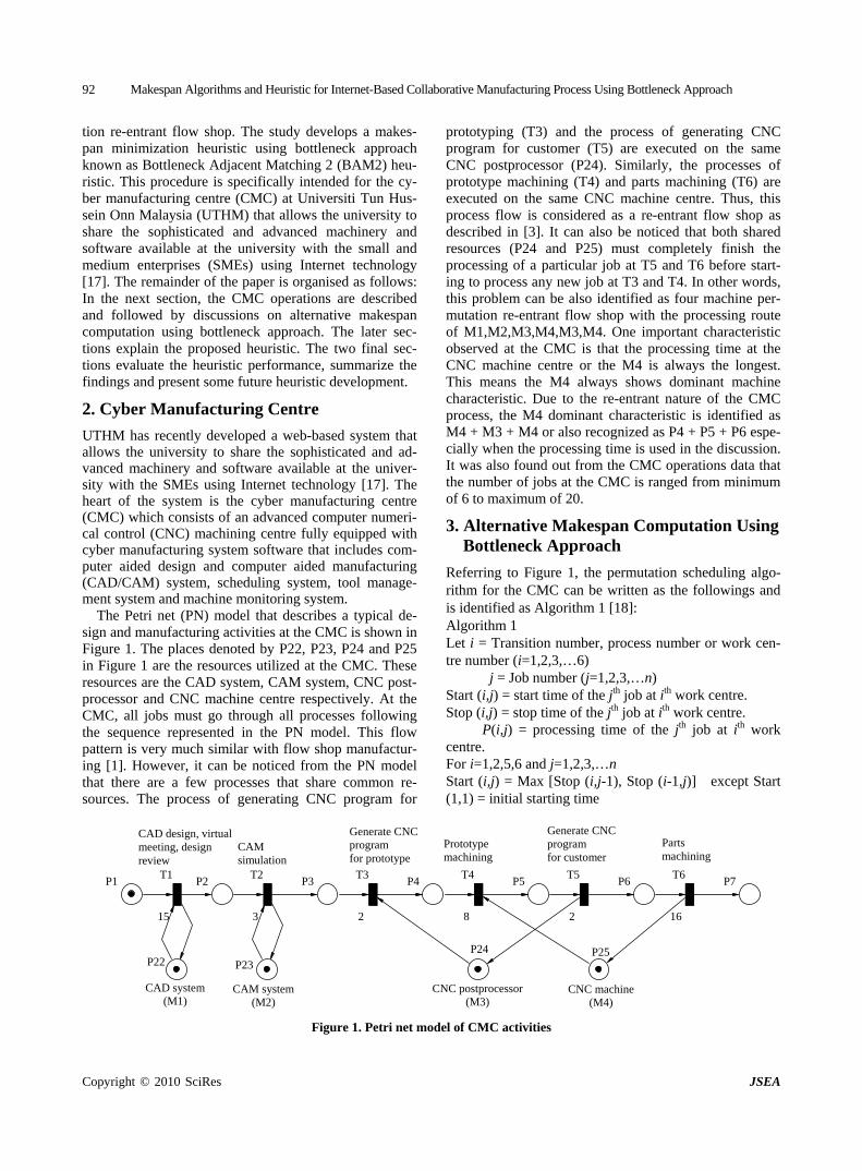
Makespan Algorithms and Heuristic for Internet-Based Collaborative Manufacturing Process Using Bottleneck Approach 92
tion re-entrant flow shop. The study develops a makes- pan minimization heuristic using bottleneck approach known as Bottleneck Adjacent Matching 2 (BAM2) heu-ristic. This procedure is specifically intended for the cy-ber manufacturing centre (CMC) at Universiti Tun Hus-sein Onn Malaysia (UTHM) that allows the university to share the sophisticated and advanced machinery and software available at the university with the small and medium enterprises (SMEs) using Internet technology [17]. The remainder of the paper is organised as follows: In the next section, the CMC operations are described and followed by discussions on alternative makespan computation using bottleneck approach. The later sec-tions explain the proposed heuristic. The two final sec-tions evaluate the heuristic performance, summarize the findings and present some future heuristic development.
2. Cyber Manufacturing Centre
UTHM has recently developed a web-based system that allows the university to share the sophisticated and ad-vanced machinery and software available at the univer-sity with the SMEs using Internet technology [17]. The heart of the system is the cyber manufacturing centre (CMC) which consists of an advanced computer numeri-cal control (CNC) machining centre fully equipped with cyber manufacturing system software that includes com-puter aided design and computer aided manufacturing (CAD/CAM) system, scheduling system, tool manage-ment system and machine monitoring system.
The Petri net (PN) model that describes a typical de-sign and manufacturing activities at the CMC is shown in Figure 1. The places denoted by P22, P23, P24 and P25 in Figure 1 are the resources utilized at the CMC. These resources are the CAD system, CAM system, CNC post-processor and CNC machine centre respectively. At the CMC, all jobs must go through all processes following the sequence represented in the PN model. This flow pattern is very much similar with flow shop manufactur-ing [1]. However, it can be noticed from the PN model that there are a few processes that share common re-sources. The process of generating CNC program for
prototyping (T3) and the process of generating CNC program for customer (T5) are executed on the same CNC postprocessor (P24). Similarly, the processes of prototype machining (T4) and parts machining (T6) are executed on the same CNC machine centre. Thus, this process flow is considered as a re-entrant flow shop as described in [3]. It can also be noticed that both shared resources (P24 and P25) must completely finish the processing of a particular job at T5 and T6 before start-ing to process any new job at T3 and T4. In other words, this problem can be also identified as four machine per-mutation re-entrant flow shop with the processing route of M1,M2,M3,M4,M3,M4. One important characteristic observed at the CMC is that the processing time at the CNC machine centre or the M4 is always the longest. This means the M4 always shows dominant machine characteristic. Due to the re-entrant nature of the CMC process, the M4 dominant characteristic is identified as M4 + M3 + M4 or also recognized as P4 + P5 + P6 espe-cially when the processing time is used in the discussion. It was also found out from the CMC operations data that the number of jobs at the CMC is ranged from minimum of 6 to maximum of 20.
3. Alternative Makespan Computation Using Bottleneck Approach
Referring to Figure 1, the permutation scheduling algo-rithm for the CMC can be written as the followings and is identified as Algorithm 1 [18]: Algorithm 1 Let i = Transition number, process number or work cen-tre number (i=1,2,3,…6) j = Job number (j=1,2,3,…n) Start (i,j) = start time of the jth job at ith work centre. Stop (i,j) = stop time of the jth job at ith work centre. P(i,j) = processing time of the jth job at ith work centre. For i=1,2,5,6 and j=1,2,3,…n Start (i,j) = Max [Stop (i,j-1), Stop (i-1,j)] except Start (1,1) = initial starting time
Figure 1. Petri net model of CMC activities
P1 P2 P3 P4 P5 P6 P7
P22 P23P24 P25
T1
15
T2
3
T3
2
T4
8
T5
2
T6
16
CAD design, virtual CAM simulation
Generate CNCprogram for prototype
Generate CNC Parts machining
Prototype machining
program for customer
meeting, design review
CAD system (M1)
CNC postprocessor(M3)
CAM system (M2)
CNC machine (M4)
Copyright © 2010 SciRes JSEA
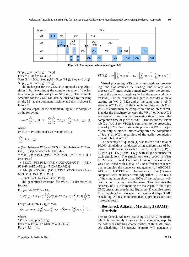
Makespan Algorithms and Heuristic for Internet-Based Collaborative Manufacturing Process Using Bottleneck Approach 93
Resource Time
M1 P11 P12 P13 P14
M2 P21
VP21
P22 VP22
P23 VP23
P24
M3 P 31
P 51
P32 P52 P33 P53 P34 P54
M4 P 41
P61
P42 P62 P43 P63 P44 P64
Figure 2. Example schedule focusing on M4 Stop (i,j) = Start (i,j) + P (i,j) For i =3,4 and j=1,2,3,…n Start (i,j) = Max [Stop (i,j-1), Stop (i-1,j), Stop (i+2,j-1)] Stop (i,j) = Start (i,j) + P(i,j)
The makespan for the CMC is computed using Algo-rithm 1 by determining the completion time of the last task belongs to the last job or Stop (6,n). The example schedule for the CMC can also be observed by focusing on the M4 as the dominant machine and this is shown in Figure 2.
The makespan for the example in Figure 2 is computed as the following:
Cmax= + 1) 3 6
1 1 4
( ,1) ( , )n
i j i
P i P i j
2
4 (n
j
P BCF j ) (
)
6
2
1
1
1
where P4BCF = P4 Bottleneck Correction Factor
2
4 (n
j
P BCF j
= (Gap between P61 and P42) + (Gap between P62 and P43) + (Gap between P63 and P44) = Max[0, P32-P61, (VP21+P22+P32) - (P21+P31+P41+ P51+P61)] + Max[0, P33-P62, (VP21+VP22+P23+P33) - (P21+ P31+P41+P51+P61) - (P42+P52+P62)] + Max[0, P34-P63, (VP21+VP22+VP23+P24+P34) - (P21+P31+P41+P51+P61) - (P42+P52+P62+ P43+P53+P63)]
The generalised equation for P4BCF is described as follows:
For j=2, P4BCF(j) = Max
(2) 3
2
0, (3, ) (6, 1) , ( , ) (2, 1) ( .1)i i
P j P j P i j VP j P i
For j=3,4..n, P4BCF(j) = Max
(3) 13 6 6
2 1 2 4 2
0, (3, ) (6, 1) , ( , ) (2, ) ( .1) ( , )j j
i k i i k
P j P j P i j VP k P i P i k
where, VP = Virtual processing For j = 1, VP(2,1) = Max [P(2,1), P(1,2)] For j = 2,3…n-1,
VP(2,j)=1 1
1 2
(2, ) (2, ), (1, ) (2, )j j j
k k k
Max VP k P j P k VP k
(4)
Virtual processing (VP) time is an imaginary process-ing time that assumes the starting time of any work process (WP) must begin immediately after the comple-tion of the previous imaginary WP at the same work cen-tre (WC). For the example in Figure 2, consider a job X starting on WC 2 (P22) and at the same time a job Y starts at WC 1 (P13). If the completion time of job X on WC 2 is earlier than the completion time of job Y at WC 1, under the imaginary concept, the VP of job X at WC 2 is extended from its actual processing time to match the completion time of job Y at WC 1. This means the VP of job X at WC 2 (or VP22) is equivalent to the processing time of job Y at WC 1 since the process at WC 2 for job Y can only be started immediately after the completion of Job Y at WC 1 regardless of the earlier completion time of job X at WC 2.
The accuracy of Equation (1) was tested with a total of 10,000 simulations conducted using random data of be-tween 1 to 80 hours for each of P( 1, j ), P( 2, j ), P( 3, j ), P( 4, j ), P( 5, j ) and P( 6, j) with six job sequence for each simulations. The simulations were coded in VBA for Microsoft Excel. Each set of random data obtained was also tested with a total of 720 different sequences that resembles the sequence arrangement of ABCDEF, ABCDFE, ABCEDF etc. The makespan from (1) were compared with makespan from Algorithm 1. The result of the simulation shows that 100% of the makespan val-ues for both methods are the same. This indicates the accuracy of (1) in computing the makespan of the 6 job CMC operations scheduling. Equation (1) was also tested for computing the makespan for 10-job and 20-job CMC scheduling. All results indicate that (1) produces accurate makespan result.
4. Bottleneck Adjacent Matching 2 (BAM2) Heuristic
The Bottleneck Adjacent Matching 2 (BAM2) heuristic, which is thoroughly illustrated in this section, exploits the bottleneck limiting characteristics of the CMC proc-ess scheduling. The BAM2 heuristic will generate a
Copyright © 2010 SciRes JSEA
Makespan Algorithms and Heuristic for Internet-Based Collaborative Manufacturing Process Using Bottleneck Approach 94
schedule which selects a job based on the best matching index to the previous job bottleneck processing time, which is the P4 + P5 + P6 (or P456) of the previous job. Ultimately, this minimizes the discontinuity time be-tween the bottleneck machines and thus produces near-optimal schedule arrangement. The procedures to implement the BAM2 heuristic to the CMC scheduling are as the followings:
Step 1: Select the job with the smallest value of P(1,j) + P(2,j)
+ P(3,j) as the first job. If more than one job are having the same smallest value of P(1,j) + P(2,j) + P(3,j), select the first job found to have the smallest P(1,j) + P(2,j) + P(3,j) value. This step is in accordance with (1), which indicated that minimum makespan can be achieved by assigning small-est P(1,j) + P(2,j) + P(3,j) as first job.
Step 2: Compute the BAM2 index for the potential second job
selection by testing each of the remaining jobs as the second job. The BAM2 indexes are derived from the P4BCF algorithm as in (2) and (3) and are computed as the followings:
For j =2, BAM2 index=
Max (5) 3
2
(3, ) (6, 1) , ( , ) (2, 1) ( .1)i
P j P j P i j VP j P i
6
2i
1j
)
For j = 3,4,..n, BAM2 index= Max
13 6 6
2 1 2 4 2
(3, ) (6, 1) , ( , ) (2, ) ( .1) ( , )j
i k i i k
P j P j P i j VP k P i P i k
(6)
where j = remaining jobs to be selected one after the other j-1 = the immediate preceding job that has been assigned The value of VP is computed using (4).
Step 3: Select the job that has zero BAM2 index. If no zero
BAM2 index is available, select the job that has the larg-est negative BAM2 index (negative BAM1 index closest to zero). If no negative BAM2 index is available, select the job with the smallest positive BAM2 index. Assign this job for the current job scheduling. If more than one job have the same best index value, select the first job found to have the best index value from the jobs list.
Step 4: Compute the BAM2 index for job scheduling assign-
ment number 3, 4….n-1 one after the other using algo-rithm at Step 2 and select the best job allocation using Step 3. Assign the last remaining job as the last job.
Step 5: Compute the makespan of the completed job schedul-
ing sequence using (1). Step 6: For the first completed schedule only, use the bottle-
neck scheduling performance 2 (BSP2) index to evaluate the schedule performance. This index is computed as the followings:
BSP2 index = + (7) 3
1
( ,1)i
P i
2
4 (n
j
P BCF j
Excluding the first job in the completed schedule,
identify other jobs which have the value of
less than the BSP2 index. Assign these jobs one after the other as the first job and repeat Step 2 to Step 5.
3
1
( , )i
P i j
Step 7: From the completed schedule arrangement list, select
the schedule that produces the minimum makespan as the BAM2 heuristic solution.
5. BAM2 Heuristic Performance Evaluation
This section discusses the BAM2 heuristic performance evaluation under a few selected operating conditions. Since the P456 dominance level is the major characteris-tic being considered in developing the BAM2 heuristic, it is appropriate to test the performance of this heuristic under various groups of dominance level values. The dominance level is measured by observing how many times the value of P2+P3+P4+P5+P6 of any job greater than P1+P2+P3 of other jobs. Similar to [13], the domi-nance level groups are divided into levels of weak P456 dominance, medium P456 dominance and strong P456 dominance. The determination of the group dominance level ranges is solely depended on the value of the maximum possible P456 dominance level divided by 3. For the experimentation that uses 6 job analysis, the maximum possible P456 dominance level equals to (n-1)n = (6-1)6 = 30. The P456 dominance level range values are summarised in Table 1.
The performance evaluation was simulated using groups of 6 jobs waiting to be scheduled at the CMC. The selection of 6 jobs enables fast enumeration of all possible job sequences that can be used to compare with the BAM2 heuristic result. The processing time for each process was randomly generated using uniform distribu-tion pattern on the realistic data ranges as in Table 2. During each simulation, data on P1 dominance level, minimum makespan from BAM2 heuristic and optimum makespan from complete enumeration were recorded. The ratio between BAM2 heuristic makespan and the optimum makespan from enumeration was then com-puted for performance measurement. A total of 3000 simulations were conducted using the randomly gener-ated data and the results are tabulated in Table 3.
The average makespan ratio in Table 3 represents the average ratio of the makespan from BAM2 heuristic to the optimum makespan from complete enumeration. The optimum result column registers the percentage of oc-
Copyright © 2010 SciRes JSEA
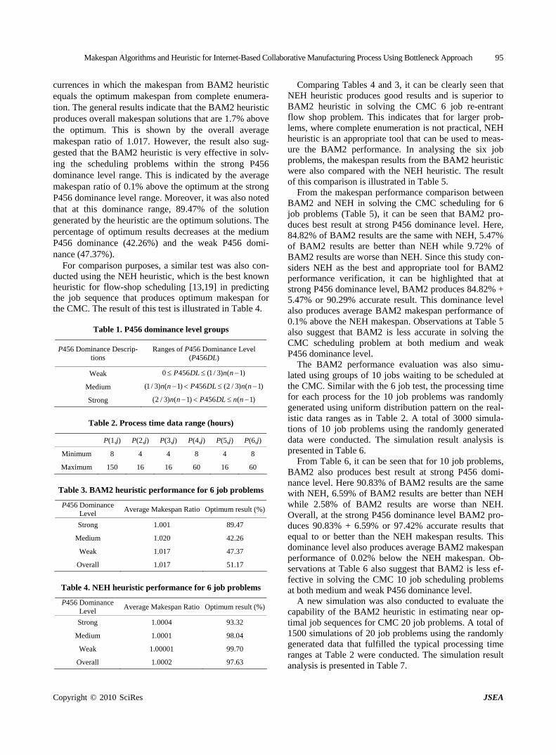
Makespan Algorithms and Heuristic for Internet-Based Collaborative Manufacturing Process Using Bottleneck Approach 95
currences in which the makespan from BAM2 heuristic equals the optimum makespan from complete enumera-tion. The general results indicate that the BAM2 heuristic produces overall makespan solutions that are 1.7% above the optimum. This is shown by the overall average makespan ratio of 1.017. However, the result also sug-gested that the BAM2 heuristic is very effective in solv-ing the scheduling problems within the strong P456 dominance level range. This is indicated by the average makespan ratio of 0.1% above the optimum at the strong P456 dominance level range. Moreover, it was also noted that at this dominance range, 89.47% of the solution generated by the heuristic are the optimum solutions. The percentage of optimum results decreases at the medium P456 dominance (42.26%) and the weak P456 domi-nance (47.37%).
For comparison purposes, a similar test was also con-ducted using the NEH heuristic, which is the best known heuristic for flow-shop scheduling [13,19] in predicting the job sequence that produces optimum makespan for the CMC. The result of this test is illustrated in Table 4.
Table 1. P456 dominance level groups
P456 Dominance Descrip-tions
Ranges of P456 Dominance Level (P456DL)
Weak 0 456 (1 / 3) ( 1P DL n n )
Medium (1/ 3) ( 1) 456 (2 / 3) ( 1)n n P DL n n
Strong (2 / 3) ( 1) 456 ( 1)n n P DL n n
Table 2. Process time data range (hours)
P(1,j) P(2,j) P(3,j) P(4,j) P(5,j) P(6,j)
Minimum 8 4 4 8 4 8
Maximum 150 16 16 60 16 60
Table 3. BAM2 heuristic performance for 6 job problems
P456 Dominance Level
Average Makespan Ratio Optimum result (%)
Strong 1.001 89.47
Medium 1.020 42.26
Weak 1.017 47.37
Overall 1.017 51.17
Table 4. NEH heuristic performance for 6 job problems
P456 Dominance Level
Average Makespan Ratio Optimum result (%)
Strong 1.0004 93.32
Medium 1.0001 98.04
Weak 1.00001 99.70
Overall 1.0002 97.63
Comparing Tables 4 and 3, it can be clearly seen that NEH heuristic produces good results and is superior to BAM2 heuristic in solving the CMC 6 job re-entrant flow shop problem. This indicates that for larger prob-lems, where complete enumeration is not practical, NEH heuristic is an appropriate tool that can be used to meas-ure the BAM2 performance. In analysing the six job problems, the makespan results from the BAM2 heuristic were also compared with the NEH heuristic. The result of this comparison is illustrated in Table 5.
From the makespan performance comparison between BAM2 and NEH in solving the CMC scheduling for 6 job problems (Table 5), it can be seen that BAM2 pro-duces best result at strong P456 dominance level. Here, 84.82% of BAM2 results are the same with NEH, 5.47% of BAM2 results are better than NEH while 9.72% of BAM2 results are worse than NEH. Since this study con-siders NEH as the best and appropriate tool for BAM2 performance verification, it can be highlighted that at strong P456 dominance level, BAM2 produces 84.82% + 5.47% or 90.29% accurate result. This dominance level also produces average BAM2 makespan performance of 0.1% above the NEH makespan. Observations at Table 5 also suggest that BAM2 is less accurate in solving the CMC scheduling problem at both medium and weak P456 dominance level.
The BAM2 performance evaluation was also simu-lated using groups of 10 jobs waiting to be scheduled at the CMC. Similar with the 6 job test, the processing time for each process for the 10 job problems was randomly generated using uniform distribution pattern on the real-istic data ranges as in Table 2. A total of 3000 simula-tions of 10 job problems using the randomly generated data were conducted. The simulation result analysis is presented in Table 6.
From Table 6, it can be seen that for 10 job problems, BAM2 also produces best result at strong P456 domi-nance level. Here 90.83% of BAM2 results are the same with NEH, 6.59% of BAM2 results are better than NEH while 2.58% of BAM2 results are worse than NEH. Overall, at the strong P456 dominance level BAM2 pro-duces 90.83% + 6.59% or 97.42% accurate results that equal to or better than the NEH makespan results. This dominance level also produces average BAM2 makespan performance of 0.02% below the NEH makespan. Ob-servations at Table 6 also suggest that BAM2 is less ef-fective in solving the CMC 10 job scheduling problems at both medium and weak P456 dominance level.
A new simulation was also conducted to evaluate the capability of the BAM2 heuristic in estimating near op-timal job sequences for CMC 20 job problems. A total of 1500 simulations of 20 job problems using the randomly generated data that fulfilled the typical processing time ranges at Table 2 were conducted. The simulation result analysis is presented in Table 7.
Copyright © 2010 SciRes JSEA
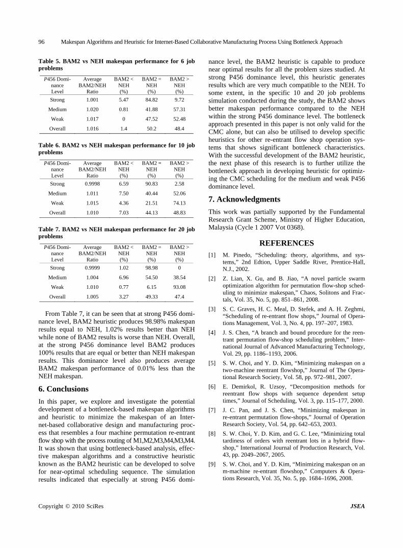
Makespan Algorithms and Heuristic for Internet-Based Collaborative Manufacturing Process Using Bottleneck Approach 96
Table 5. BAM2 vs NEH makespan performance for 6 job problems
P456 Domi-nance Level
Average BAM2/NEH
Ratio
BAM2 < NEH (%)
BAM2 = NEH (%)
BAM2 > NEH (%)
Strong 1.001 5.47 84.82 9.72
Medium 1.020 0.81 41.88 57.31
Weak 1.017 0 47.52 52.48
Overall 1.016 1.4 50.2 48.4
Table 6. BAM2 vs NEH makespan performance for 10 job problems
P456 Domi-nance Level
Average BAM2/NEH
Ratio
BAM2 < NEH (%)
BAM2 = NEH (%)
BAM2 > NEH (%)
Strong 0.9998 6.59 90.83 2.58
Medium 1.011 7.50 40.44 52.06
Weak 1.015 4.36 21.51 74.13
Overall 1.010 7.03 44.13 48.83
Table 7. BAM2 vs NEH makespan performance for 20 job problems
P456 Domi-nance Level
Average BAM2/NEH
Ratio
BAM2 < NEH (%)
BAM2 = NEH (%)
BAM2 > NEH (%)
Strong 0.9999 1.02 98.98 0
Medium 1.004 6.96 54.50 38.54
Weak 1.010 0.77 6.15 93.08
Overall 1.005 3.27 49.33 47.4
From Table 7, it can be seen that at strong P456 domi-
nance level, BAM2 heuristic produces 98.98% makespan results equal to NEH, 1.02% results better than NEH while none of BAM2 results is worse than NEH. Overall, at the strong P456 dominance level BAM2 produces 100% results that are equal or better than NEH makespan results. This dominance level also produces average BAM2 makespan performance of 0.01% less than the NEH makespan.
6. Conclusions
In this paper, we explore and investigate the potential development of a bottleneck-based makespan algorithms and heuristic to minimize the makespan of an Inter-net-based collaborative design and manufacturing proc-ess that resembles a four machine permutation re-entrant flow shop with the process routing of M1,M2,M3,M4,M3,M4. It was shown that using bottleneck-based analysis, effec-tive makespan algorithms and a constructive heuristic known as the BAM2 heuristic can be developed to solve for near-optimal scheduling sequence. The simulation results indicated that especially at strong P456 domi-
nance level, the BAM2 heuristic is capable to produce near optimal results for all the problem sizes studied. At strong P456 dominance level, this heuristic generates results which are very much compatible to the NEH. To some extent, in the specific 10 and 20 job problems simulation conducted during the study, the BAM2 shows better makespan performance compared to the NEH within the strong P456 dominance level. The bottleneck approach presented in this paper is not only valid for the CMC alone, but can also be utilised to develop specific heuristics for other re-entrant flow shop operation sys-tems that shows significant bottleneck characteristics. With the successful development of the BAM2 heuristic, the next phase of this research is to further utilize the bottleneck approach in developing heuristic for optimiz-ing the CMC scheduling for the medium and weak P456 dominance level.
7. Acknowledgments
This work was partially supported by the Fundamental Research Grant Scheme, Ministry of Higher Education, Malaysia (Cycle 1 2007 Vot 0368).
REFERENCES [1] M. Pinedo, “Scheduling: theory, algorithms, and sys-
tems,” 2nd Edtion, Upper Saddle River, Prentice-Hall, N.J., 2002.
[2] Z. Lian, X. Gu, and B. Jiao, “A novel particle swarm optimization algorithm for permutation flow-shop sched-uling to minimize makespan,” Chaos, Solitons and Frac-tals, Vol. 35, No. 5, pp. 851–861, 2008.
[3] S. C. Graves, H. C. Meal, D. Stefek, and A. H. Zeghmi, “Scheduling of re-entrant flow shops,” Journal of Opera-tions Management, Vol. 3, No. 4, pp. 197–207, 1983.
[4] J. S. Chen, “A branch and bound procedure for the reen-trant permutation flow-shop scheduling problem,” Inter-national Journal of Advanced Manufacturing Technology, Vol. 29, pp. 1186–1193, 2006.
[5] S. W. Choi, and Y. D. Kim, “Minimizing makespan on a two-machine reentrant flowshop,” Journal of The Opera-tional Research Society, Vol. 58, pp. 972–981, 2007.
[6] E. Demirkol, R. Uzsoy, “Decomposition methods for reentrant flow shops with sequence dependent setup times,” Journal of Scheduling, Vol. 3, pp. 115–177, 2000.
[7] J. C. Pan, and J. S. Chen, “Minimizing makespan in re-entrant permutation flow-shops,” Journal of Operation Research Society, Vol. 54, pp. 642–653, 2003.
[8] S. W. Choi, Y. D. Kim, and G. C. Lee, “Minimizing total tardiness of orders with reentrant lots in a hybrid flow-shop,” International Journal of Production Research, Vol. 43, pp. 2049–2067, 2005.
[9] S. W. Choi, and Y. D. Kim, “Minimizing makespan on an m-machine re-entrant flowshop,” Computers & Opera-tions Research, Vol. 35, No. 5, pp. 1684–1696, 2008.
Copyright © 2010 SciRes JSEA
Makespan Algorithms and Heuristic for Internet-Based Collaborative Manufacturing Process Using Bottleneck Approach
Copyright © 2010 SciRes JSEA
97
[10] J. S. Chen, J. C. H. Pan, and C. K. Wu, “Hybrid tabu search for re-entrant permutation flow-shop scheduling problem. Expert Systems with Applications,” Vol. 34, No. 3, pp. 1924–1930, 2008.
[11] J. S. Chen, J. C. H. Pan, and C. M.Lin, “Hybrid genetic algorithm for the re-entrant flow-shop scheduling prob-lem. Expert Systems with Applications,” Vol. 34, pp. 570–577, 2008.
[12] S. Mukherjee, and A. K. Chatterjee, “Applying machine based decomposition in 2-machine flow shops,” European Journal of Operational Research, Vol. 169, pp. 723–741, 2006.
[13] A. A. Kalir , and S. C. Sarin, “A near optimal heuristic for the sequencing problem in multiple-batch flow-shops with small equal sublots,” Omega, Vol. 29, pp. 577–584, 2001.
[14] J. B. Wang, F. Shan, B. Jiang, and L. Y. Wang, “Permu-tation flow shop scheduling with dominant machines to minimize discounted total weighted completion time,” Applied Mathematics and Computation, Vol. 182, No. 1, pp. 947–957, 2006.
[15] B. C. Choi, S. H. Yoon, and S. J. Chung, “Minimizing
maximum completion time in a proportionate flow shop with one machine of different speed,” European Journal of Operational Research, Vol. 176, No. 2, pp. 964–976, 2007.
[16] M. B. Cheng, S. J. Sun, and L. M. He, “Flow shop sched-uling problems with deteriorating jobs on no-idle domi-nant machines,” European Journal of Operational Re-search, Vol. 183, pp. 115–124, 2007.
[17] S. A. Bareduan, S. H. Hasan, N. H. Rafai, and M. F. Shaari, “Cyber manufacturing system for small and me-dium enterprises: a conceptual framework,” Transactions of North American Manufacturing Research Institution for Society of Manufacturing Engineers, Vol. 34, pp. 365–372, 2006.
[18] S. A. Bareduan, S. H. Hasan, and S. Ariffin, “Finite scheduling of collaborative design and manufacturing ac-tivity: a Petri net approach,” Journal of Manufacturing Technology Management, Vol. 19, No. 2, pp. 274–288, 2008.
[19] P. J. Kalczynski, and J. Kamburowski, “On the NEH heuristic for minimizing the makespan in permutation flow shops,” Omega, Vol. 35, pp. 53–60, 2007.


![PARALLEL C-MEANS ALGORITHM FOR IMAGE SEGMENTATION ON A RECONFIGURABLE MESH …fs.unm.edu/ScPr/ParallelCMeansAlgorithm.pdf · 2017. 9. 1. · [23] M. Youssfi, O. Bouattane, M.O. Bensalah,](https://img.pdfslide.us/doc/110x75/60b437c0acb6f31bf864a775/parallel-c-means-algorithm-for-image-segmentation-on-a-reconfigurable-mesh-fsunmeduscprpar.jpg)