Copyright © 2009, 2010 by Robin Greenwood and Samuel Hanson

Working papers are in draft form. This working paper is distributed for purposes of comment and discussion only. It may not be reproduced without permission of the copyright holder. Copies of working papers are available from the author.

Characteristic Timing Robin Greenwood Samuel Hanson

Working Paper

09-099

Electronic copy available at: http://ssrn.com/abstract=1320187

Characteristic Timing∗

Robin Greenwood

Harvard Business School and NBER rgreenwood@hbs.edu

Samuel Hanson Harvard University shanson@hbs.edu

Revised: February 2010 (First draft: November 2008)

Abstract We use differences between the attributes of stock issuers and repurchasers to forecast characteristic-related stock returns. For example, we show that large firms underperform following years when issuing firms are large relative to repurchasing firms. Our approach is useful for forecasting returns to portfolios based on book-to-market (HML), size (SMB), price, distress, payout policy, profitability, and industry. We consider interpretations of these results based on both time-varying risk premia and mispricing. Our results are primarily consistent with the view that firms issue and repurchase shares to exploit time-varying characteristic mispricing.

∗ A previous version of this paper was titled “Catering to Characteristics.” We are grateful to Malcolm Baker, John Campbell, Sergey Chernenko, Lauren Cohen, Ben Esty, Borja Larrain, Owen Lamont, Jon Lewellen, Jeff Pontiff, Huntley Schaller, Andrei Shleifer, Erik Stafford, Jeremy Stein, Adi Sunderam, Ivo Welch, Jeff Wurgler, and seminar participants at Harvard, INSEAD, HEC, AllianceBernstein, the University of Michigan, and the NBER Behavioral Working Group for helpful suggestions. The Division of Research at the Harvard Business School provided funding.

Electronic copy available at: http://ssrn.com/abstract=1320187

I. Introduction

It is well known that firms that issue stock subsequently earn low returns on average.

Loughran and Ritter (1995) find that firms issuing equity in either an IPO or a SEO

underperform significantly post offering. Loughran and Vijh (1997) show that acquirers in stock-

financed mergers later underperform. Conversely, Ikenberry, Lakonishok and Vermaelen (1995)

find that firms repurchasing shares have abnormally high returns. Fama and French (2008a) and

Pontiff and Woodgate (2008) synthesize these results using a composite measure of net stock

issuance: they show that the change in split-adjusted shares outstanding is a strong negative

predictor of returns in the cross-section.

A reasonable and widely accepted interpretation of these facts is that managers exploit

private information about the firm’s future stock returns to minimize the total cost of financing.

Where does this informational advantage come from? One view is that managers who know that

their firm is overvalued issue shares to investors who in turn are overly optimistic about the

firm’s future performance. As Loughran and Ritter (1995) put it, “firms take advantage of

transitory windows of opportunity by issuing equity when, on average, they are substantially

overvalued.” This interpretation receives support in Graham and Harvey’s (2001) survey of

CFOs: 67 percent claim that the “the amount by which our stock is undervalued or overvalued by

the market” influences whether the firm issues equity.

In this paper, we put forth a complementary interpretation of these results: firms issue

and repurchase shares to exploit time-varying characteristic mispricing. We show that firms issue

prior to periods in which their characteristics perform poorly, and repurchase prior to periods

when their characteristics perform well. Our empirical design relies on two assumptions. First,

firm characteristics – such as the book-to-market ratio, sales growth, dividend policy, or industry

affiliation – may be correlated with future returns in the cross-section. This assumption receives

Electronic copy available at: http://ssrn.com/abstract=1320187

2

considerable support in the vast empirical literature on stock returns (e.g., Daniel and Titman

1997). Second, characteristic-based expected returns may vary over time. Variation in expected

characteristic returns may be driven by time-varying risk premia, or they may be driven by

characteristic-level mispricing. In the latter case, we might interpret characteristic-level

mispricing as stemming from time-varying investor enthusiasm for different themes. Together,

these assumptions amount to saying that stock returns can be described by a conditional

characteristics model.

How should firms respond to predictable variation in characteristic returns? If this

variation reflects mispricing, firms endowed with a characteristic with low expected returns can

exploit this by selling shares or undertaking stock-financed acquisitions. This activity advantages

firms’ existing long-term shareholders at the expense of short-term investors who buy shares

which subsequently underperform. Likewise, firms endowed with a characteristic with high

expected returns may decide to repurchase existing shares. Why do firms undertake trades of this

sort? Relative to professional arbitrageurs, firms may be advantaged when mispricing converges

slowly or is associated with undiversifiable risk (e.g., Shleifer and Vishny 1997; Stein 2005).

Following the logic above, differences between the attributes of recent issuers and

repurchasers can be used to forecast characteristic-level returns. So, for example, if we were to

observe that recent issuers were predominately firms with characteristic X, we might reasonably

infer that returns of firms with characteristic X would subsequently be low. As we discuss below,

the characteristics of recent issuers might be useful for forecasting characteristic returns even if

this is driven solely by rational variation in risk premia.

Our empirical strategy closely follows the above intuition. Focusing on firm attributes

identified by previous work, we use differences between the characteristics of recent issuers and

repurchasers – which we call “issuer-repurchaser spreads” – to forecast returns to long-short

3

portfolios associated with these characteristics. Specifically, following periods in which issuing

firms have particularly high values of a characteristic compared to repurchasing firms, we would

expect the long-short portfolio associated with that characteristic to perform poorly. Which firm

attributes? Although in principle our approach could be applied to any characteristic, we limit

ourselves to traits which have appeared in previous work and, more importantly, can be

measured reliably in the data since the 1960s: book-to-market, sales growth, accruals, size,

nominal share price, age, beta, volatility, distress (bankruptcy hazard rate), dividend policy, and

profitability. In selecting these characteristics, we hope to capture some of the salient dimensions

along which investors categorize stocks.1

In our baseline results, characteristic issuer-repurchaser spreads significantly forecast

characteristics-based returns in six cases: book-to-market, size, nominal share price, distress,

payout policy, profitability, and industry. For the remaining characteristics, the issuer-

repurchaser spread forecasts returns negatively, albeit with reduced statistical significance. Our

measures help forecast factors associated with size (SMB) and book-to-market (HML).

Arguably, book-to-market and size are two of the most important attributes that investors use to

categorize stocks. Concretely, this means that when issuance is particularly tilted toward large

(low B/M) stocks, SMB (HML) is expected to perform well in the subsequent year. In short,

firms appear to be successful factor timers.

One objection to the results described so far is that we may be picking up a time-varying

loading on the net-issuance anomaly itself—and thus simply repackaging the known relationship

between equity issuance and future stock returns. For instance, if one takes the 1 Among the characteristics listed above, book-to-market, size, nominal share price, dividend payout policy, and industry stand out as being most relevant from the perspective of investor categorization. For instance, there are mutual funds dedicated to stocks in each of these categories. For some of the other characteristics, such as profitability or sales growth, it is less clear that they form the basis of any particular investment style, yet some authors (e.g., Aghion and Stein (2008)) have argued that they may be salient at particular times. Barberis and Shleifer (2003) develop a model in which investors categorize stocks into styles.

4

underperformance of net-issuers as a primitive fact, then it might not be surprising to find that

HML performs well when growth firms have recently issued stock, or likewise, when value firms

have recently repurchased stock. This concern turns out to be easy to fix: similar to Loughran

and Ritter (2000) we construct long-short characteristic portfolios that exclude the issuing and

repurchasing firms. We achieve essentially similar results using these “issuer-purged” portfolios.

In summary, net issuance forecasts the returns of non-issuing firms with similar characteristics.

In a separate set of tests, we examine industry-related characteristics and find that the issuance

and repurchase decisions of firms in a given industry forecast the returns to non-issuers in the

same industry.

An important question is whether our results are consistent with market efficiency. We

consider two potential explanations. The first is that, because equity issues have the effect of

delevering the firm’s assets, the required returns on equity falls mechanically post issuance

through a Modigliani and Miller (1958) channel. A variation of this explanation is that issuance

causes lower returns because firms convert growth options into assets in place when they decide

to invest (Carlson, Fisher, Giammarino 2004). Because growth options are riskier than installed

assets, required returns fall post-issuance. These explanations are unable to account for our

results because issuer-repurchaser spreads forecast characteristic returns for firms that do not

issue or repurchase.

A second potential explanation is that issuance is a noisy proxy for investment which

responds to time variation in rationally required returns. Specifically, when rationally required

returns decline, firms will invest more and some of this investment will be financed with

additional equity. Under this explanation, issuer-repurchaser spreads forecast characteristic

returns because a higher value of the characteristic among issuing firms is associated with lower

required returns. However, in this case, the difference in characteristics between firms with high

5

and low levels of investment should be a better forecaster of returns than the issuer-repurchaser

spread. In univariate regressions these investment-based measures have some modest ability to

predict characteristic-level returns. However, in horse races with our issuer-repurchaser spreads,

the issuer-repurchaser spreads generally remain significant while the investment-based measures

often enter with the wrong sign and are rarely statistically insignificant.

In summary, the evidence is primarily consistent with the view that issuance and

repurchase activity is partly an attempt to exploit time-varying characteristic mispricing,

suggesting that firms may play a role as arbitrageurs in the capital market. We stress, however,

that our forecasting results are useful even if they are consistent with some forms of market

efficiency, since they help us forecast time-series variation in returns at the characteristic level.

For instance, other than Cohen, Polk, and Vuolteenaho (2003), we know of no other paper that

has had much empirical success forecasting HML or SMB.

Given these results, we ask what fraction of the underperformance of recent issuers can

be explained by characteristic timing. If firms only respond weakly to time-varying expected

characteristic returns, characteristic timing might be relatively unimportant from a corporate

finance standpoint, although still useful for forecasting returns. Our estimates suggest that at

least one fifth of the underperformance of recent issuers is due to characteristic timing.

The paper proceeds as follows. In the next section, we lay out an empirical model of

characteristic timing. Section III describes the construction of our characteristic issuer-

repurchaser spread measures. In Section IV, we use issuer-repurchaser spreads to forecast

returns. Section V considers whether the results are consistent with market efficiency, or whether

they are better explained by the view that firms time their issuance to exploit mispriced

characteristics. Section VI evaluates the economic importance of characteristic timing from the

point of view of corporate issuance. The final section concludes.

6

II. Empirical strategy

We develop a framework to motivate our empirical strategy, which uses patterns in

corporate issuance to identify time-variation in characteristic expected returns. We assume that

expected returns are given by a conditional characteristics model:

1 , 1 1 , 1 2 1 , 1 , 1( )t i t t i t t i t i tE R X T Xα β β µ− − − − − − = + ⋅ + ⋅ × + (1)

where Xi,t-1 denotes firm i’s characteristic and Tt-1 reflects time-series variation in the conditional

expected return associated with that characteristic. We emphasize that at this point it makes no

difference if we interpret time-series variation in expected characteristic returns as reflecting

mispricing (in which case they are deviations from rationally required returns) or if (1) describes

investors’ required returns. In the first case, equation (1) can be seen as a stylized representation

of the idea that investor sentiment is associated with different themes during different periods.

Themes attach themselves to attributes, such as “internet,” “profitable,” “large stocks,” or “high

dividend yield” but we recognize that the mapping between these themes and the characteristics

we measure in the data is inherently imperfect. Baker and Wurgler (2006) use a similar empirical

specification to study the role of time-varying investor sentiment. Equation (1) can also be

interpreted within the context of rationally time-varying risk premia: in this case, we assume that

characteristic X is related to the firm’s loading on some risk factor whose price of risk (T) varies

over time.

To keep matters simple, we write equation (1) as a function of a single characteristic.

Without loss of generality, we also assume that E[Tt-1]=0, so that β1 represents the average cross-

sectional effect of Xi,t-1 (e.g., the average premium associated with size) and that Xi,t-1 and Tt-1 are

independent. µi,t-1 is identically and independently distributed over time and across firms, with

7

mean zero and variance 2µσ . This term captures the idea that expected returns can only partially

be explained by the characteristic under investigation.

We assume that corporations issue stock when expected returns are low and repurchase

when expected returns are high. Thus, net stock issuance (NS) is given by

, 1 1 , , 1i t t i t i tNS E R ε− − − = − + (2)

where εi,t-1 is independently distributed across time and firms. We assume a unit elasticity of net

issuance with respect to expected returns for simplicity only. Equation (2) can be seen as a

reduced form representation of the idea that managers derive some benefit from issuing

overpriced equity (and likewise, benefit from repurchasing underpriced equity).2 Under this

interpretation, the noise term ε captures all factors other than market timing that may influence

net stock issuance. For example, some firms might like to exploit mispricing, but can or do not

for idiosyncratic reasons. The larger is the variance of ε, the smaller is the role of market timing

in explaining net stock issuance.3

2As long as mispricing eventually reverts, such opportunistic issuance benefits long-term shareholders at the expense of short-term shareholders who buy the mispriced securities. Shleifer and Vishny (2003) and Baker, Ruback and Wurgler (2007) discuss this in more detail.

Equation (2) can also be interpreted within a fully rational

paradigm in which firms invest more and, hence, issue more equity when rationally required

returns fall. In this case, the noise term ε captures the fact that equity issuance is only a noisy

signal of investment because it reflects a series of uninformative decisions about how that

investment should be financed. In the Appendix, we present a short model in the spirit of Stein

(1996) that motivates equation (2) and nests rational interpretations and interpretations based on

3 For simplicity, equation (2) does not consider feedback effects of issuance on future returns. In Greenwood, Hanson, and Stein (2010), for example, firms issue more when expected returns are low, but in equilibrium, firms “fill the gap,” reducing predictability. Another assumption implicit in (2) is that firms respond with the same intensity to mispricing in any given period.

8

mispricing. Specifically, in this model, issuance is negatively related to both mispricing and to

rational time-varying returns.

Substituting (1) into (2), we have

, 1 1 1 , 1 2 1 , 1 , 1 , 1[ ( ) ] .i t t i t t i t i t i tNS X T Xα β β µ ε− − − − − − −= − + ⋅ + ⋅ × + + (3)

Equation (3) says that issuance will respond to market-wide, characteristic-specific, and firm-

specific expected returns. We now consider a univariate cross-sectional regression of issuance in

period t-1 on characteristics Xi,t-1: , 1 1 1 . 1 , 1i t t t i t i tNS Xθ δ ε− − − − −= + ⋅ + . The slope coefficient from this

regression is

1 1 2 1( )t tTδ β β− −= − + ⋅ , (4)

which is the conditional expected return associated with Xi,t-1. Assuming that β1 and β2 are fixed,

the time series of cross-sectional regression coefficients δt-1 will reveal time variation in

characteristic expected returns Tt-1. The intuition here is straightforward: while the relationship

between expected returns and individual firm issuance and repurchase decisions will be noisy,

the full cross-section of net stock issuance contains information about characteristic-level

expected returns.

The benefit of this approach is best illustrated by example: suppose we are interested in

forecasting Google’s return for the coming year. Following the literature on the cross-section of

expected stock returns, we might assemble information on Google’s characteristics (e.g. book-to-

market, size, dividend yield, profitability, industry, etc.) and construct a forecast under the

assumption that each characteristic is associated with some average return in the cross-section.

However, the previous discussion suggests a refinement. We can use the net issuance of firms

that have the same characteristics as Google to back-out Google’s expected return. Such

information is captured by 1tδ − .

9

A simple implementation of this idea is to compute differences between the

characteristics of issuers (firms with high NSi,t-1) and repurchasers (firms with low NSi,t-1); the

time-series of these differences should negatively forecast returns associated with that

characteristic. We adopt this implementation in Section III.

A more formal implementation can be seen in a panel regression of stock returns on

lagged values of the characteristic, lagged net issuance, and interactions of the lagged

characteristic with our cross-section-based estimate of characteristic expected returns (Tt-1):

, 1 , 1 2 1 , 1 , 1 ,( )i t t i t t i t i t i tR a b X b T X c NS u− − − −= + ⋅ + ⋅ × + ⋅ + (5)

Does knowledge of Tt-1 help forecast stock returns beyond a firm’s own issuance? We have

2

2 2 2 2 .b ε

µ ε

σβσ σ

=+ (6)

Thus, β2 will be non-zero as long as 2 0εσ > : our estimates of time-varying characteristic

expected returns will have incremental forecasting power so long as individual firm net issuance

is a noisy signal of expected returns.

III. Issuer-repurchaser characteristic spreads

The previous section suggests that if we measure the extent to which net issuers are

disproportionately firms endowed with a characteristic, that this should provide information

about the conditional expected returns of that characteristic. We do this for eleven

characteristics, as well as a set of industry-related attributes.

A. Calculation

10

Following Fama and French (2008a), we define net stock issuance (NS) as the change in

log split-adjusted shares outstanding from Compustat (CSHO x AJEX).

In December of year t-1, we divide all firms into New lists, Issuers, Repurchasers, and

Others (i.e., non-issuers) based on share issuance in year t-1. New lists are firms that listed

during year t-1 (these firms have Age less than one in December of year t-1). Since many of the

characteristics we study cannot be defined for new lists, we discard these firms in our baseline

measures. The remaining seasoned firms are divided into three categories: Issuers have NS

greater than 10%. Repurchasers have NS less than -0.5%, and Others have NS between -0.5%

and 10%. Since we are using a composite net issuance measure, issuers include firms completing

SEOs, stock-financed mergers, and other corporate events that significantly increase shares

outstanding (e.g. large executive compensation schemes). Figure 1 illustrates the breakdown of

NS into these three groups by showing the histogram of net issuance of public firms in 1984.

Table 2 summarizes the breakdown by year. Between 1962 and 2006, an average 6.6% of firms

were new lists, 12.4% were issuers, and 13.5% were repurchasers.

Table 2 also shows the average net issuance for firms in each group. Among issuers,

average net issuance hovered near 20% during the 1960s and 1970s, trended upwards during the

1980s, reaching a peak of 43.9% in 1993, and has declined somewhat since the early 1990s.

Repurchasers have bought back between 3% and 7% of shares, on average, since the early

1970s; however, there has been a modest trend toward smaller repurchases in recent years. Due

to growth in executive compensation, the average value of NS among non-issuers has risen

slightly from 1.1% in 1973 to 2.0% in 2006 (Fama and French 2005).

Our objective is to measure time-series variation in the composition of issuers and

repurchasers. Let , 1i tX − denote firm i’s value of (or cross-sectional decile for) characteristic X in

11

year t-1. We define the issuer-repurchaser spread for characteristic X as the average characteristic

decile of issuers minus the average characteristic decile of repurchasers:

, 1, 1

11 1

i ti t

i RepurchasersX i Issuerst Issuers Repurchasers

t t

XXISSREP

N N

−−∈∈

−− −

= −∑∑

(7)

where cross-sectional X-deciles for each year are based on NYSE breakpoints. For instance, if

we consider size (ME), then 1 1MEtISSREP− = indicates that issuing firms were on average one size

decile larger than repurchasing firms in year t-1. We define characteristic issuer-repurchaser

spreads for book-to-market equity (B/M), sales growth (ΔS t/S t-1), accruals (Acc/A), size (ME),

nominal share price (P), age, beta (β ), idiosyncratic volatility (σ), distress (SHUM) proxied

using the Shumway (2001) bankruptcy hazard rate, dividend policy (Div), and profitability (E/B).

These characteristics capture themes related to growth and growth opportunities (B/M, ΔS t/S t-1,

Acc/A), size and/or safety (ME, P, Age, β, σ, SHUM, Div), and profitability (E/B). The detailed

construction of each characteristic is described in the Appendix. All characteristics except for

dividend policy are measured using NYSE deciles; dividend policy is a dummy variable that

takes a value of one if the firm paid a cash dividend in that year. We follow the Fama and French

(1992) convention that accounting variables are measured in the fiscal year ending in year t-1

and market-based variables are measured at the end of June of year t.

Intuitively, the issuer-repurchaser spread captures the tilt of net issuance with respect to a

given characteristic. A few alternate constructions could capture the same intuition. One obvious

alternative would be to compare characteristics between new lists and existing firms. Underlying

this would be the idea that a firm’s decision to go public is affected by the conditional expected

12

returns associated with its characteristics. Not surprisingly, spreads based on the characteristics

of new lists are correlated with measures we compute in (7).4

Although we examine a variety of characteristics, a priori one might expect our approach

to work better for some characteristics than for others. One issue is that in order for ISSREPX to

forecast returns associated with characteristic X, any time variation in expected returns must be

sufficiently persistent for corporate managers to be able to act on it in a reasonable time-frame.

For instance, under the characteristic mispricing interpretation, there may be a delay between the

recognition of mispricing and managers’ ability to issue more equity. Thus, we would be

surprised to find firms timing their issuance and repurchase decisions to exploit short-lived

signals such as one-month reversal. By contrast, we would be less surprised to find firms

responding to changes in expected returns of more persistent characteristics such as B/M, size, or

industry.

When using the issuer-repurchaser spreads to forecast returns, we primarily focus on the

1972-2006 period, thus forecasting returns for 1973-2007, although we always show results for

the full 1963-2007 period as well. Our focus on the later data is for two reasons. First, we worry

that characteristic spreads are contaminated by changes in the CRSP universe due to the

introduction of NASDAQ data in December 1972. Second, Pontiff and Woodgate (2008) and

Fama and French (2008b) find that net share issuance does not predict returns prior to 1970 and

1963, respectively. Bagwell and Shoven (1989) point out that repurchases surged after 1982.

Fama and French (2005) argue that share issuance has become far more widespread post-1972,

while Fama-French (2008c) show that net issuance was more responsive to valuations (B/M) in

their 1983-2006 sub-sample than from 1963-1982.

4 We achieve many of the same results if we instead define a “new list minus repurchaser” spread constructed analogously to our main predictor. However, for several of the characteristics we consider, the new list characteristic series are noisier than our SEO-based series, driven by a few years in which the number of new lists is quite small.

13

B. Discussion

Figure 2 plots and Table 1 summarizes issuer-repurchaser spreads for each of the eleven

characteristics. Panel A of Table 3 lists the average cross-sectional correlations between our

eleven characteristics (in decile form) and Panel B of Table 3 summarizes the time-series

correlations between the eleven issuer-repurchaser spreads.

From Table 1, the average value of the issuer-repurchaser spread for book-to-market is -

1.78 deciles and is always negative, as issuers are disproportionately growth firms throughout the

sample. More importantly for our purposes, Panel A of Figure 2 shows that the issuer-

repurchaser spread for book-to-market exhibits significant time-series variation. The spread

starts out low during the “tronics” fad of 1962 and is low again during the boom of 1967-1968.

The spread is high during the bear market of the early to mid-1970s, but declines during the late

1970s and the IPO boom of the early 1980s. The spread begins to rise in 1983 and remains high

throughout the remainder of the 1980s. It then drops sharply during the technology bubble in

1999, before rising significantly afterwards.

The issuer-repurchaser spread for sales growth is always positive, indicating that issuers

have higher sales growth than repurchasers on average. Panel B of Figure 2 suggests that

issuance was particularly tilted toward firms with high sales growth during the late 1960s and

early 1970s, the early 1980s, and again in the late 1990s. The issuer-repurchaser spread for

accruals is typically positive and is highly correlated with the issuer-repurchaser spread for sales

growth (ρ = 0.72).

As shown in Panel B of Table 3, the issuer-repurchaser spreads for size, price, age, beta,

idiosyncratic volatility, and dividend policy are all strongly correlated, with pairwise correlations

ranging from 0.44 to 0.97 in magnitude.

14

The issuer-repurchaser spread for size is close to zero on average. That is, there has been

little unconditional size tilt in stock issuance. However, there is significant time-series variation.

As shown in Panel D of Figure 2, issuance was tilted toward small firms in the late 1960s and

toward large firms during the “nifty-fifty” period of the early 1970s when large firms were

popular with investors. The spread appears slightly countercyclical, increasing modestly during

each of the recessions in our sample with the exception of the 1980-1982 recession.

Greene and Hwang (2008) suggest that investors classify stocks based on their nominal

share price. Panel E shows that the issuer-repurchaser spread for share price closely tracks the

spread for size. Benartzi, Michaely, Thaler and Weld (2007) point out that size and price are

strongly correlated in the cross-section.

As shown in Panel F of Figure 2, the issuer-repurchaser spread for age also tracks the

spread for size, particularly during the first half of the sample. Consistent with Loughran and

Ritter (2004), who find little change in the age of IPO firms from 1980-1998, the age spread has

been relatively constant since the early 1980s. However, there is a small shift toward older

issuers after the collapse of technology stocks in 2000.

The issuer-repurchaser spreads for beta and volatility are highly correlated in the time-

series (ρ = 0.68). While the issuer repurchaser spread for beta is usually positive, Panel G

shows that issuance was particularly tilted towards high beta firms during the late 1960s, early

1980s, and late 1990s. The issuer-repurchaser spread for volatility is always positive and has

trended steadily upwards since the late 1970s.

The issuer-repurchaser spread for distress in part reflects the previous results for size and

volatility. Our distress measure is the bankruptcy hazard rate estimated by Shumway (2001) and

reflects a linear combination of size, volatility, past returns, profitability, and leverage. As shown

in Panel I of Figure 2, issuers typically face higher bankruptcy risks than repurchasers. Issuance

15

was tilted towards firms with high bankruptcy risk during the late 1960s and early 1970s, with

the pattern reversing in the mid-1970s. Not surprisingly, there is some tendency for the issuer-

repurchaser spread for distress to decline during recessions.

The issuer-repurchaser spread for dividend policy is highly correlated with the spreads

for size and age. This series is also 50% correlated with the Baker and Wurgler (2004) dividend

premium (untabulated). This is not surprising given the cross-sectional correlation between net

issuance and market-to-book ratios.

Last, consistent with the findings in Fama and French (2004), Panel K of Figure 2 shows

that there is a steady downward trend in the profitability of issuers relative to repurchasers.

IV. Results

In this section, we use issuer-repurchaser spreads to forecast characteristic returns. We

also consider an adjustment to our baseline methodology that allows us to consider industry-

related characteristics.

A. Long-short portfolio forecasting regressions

Our main prediction is that the long-short portfolio for a given characteristic will

underperform following periods when the issuer-repurchaser spread is high. Table 4 shows the

results from our baseline forecasting regression:

1X X

t t tR a b ISSREP u−= + ⋅ + (8)

where RX denotes the return on a portfolio that buys firms with high values of characteristic X

and sells short firms with low values of X. The construction of these portfolios follows the Fama

and French (1993) procedure for constructing HML.5

5 Firms are independently sorted into Low, Neutral, or High groups of characteristic X using 30% and 70% NYSE breakpoints, and as small or big relative to the NYSE size median. We compute value weighted returns within these

For example, if the characteristic in

16

question is B/M, then RX is simply the return on the Fama and French HML portfolio. For the

size (ME) characteristic, RX is negative one times SMB. We follow the usual timing convention

that issuer-repurchase spreads for fiscal-years ending in calendar year t-1 are matched to monthly

returns between July of year t and June of year t+1. In these monthly regressions, the ISSREPX

predictor is measured annually, so standard errors are clustered by portfolio formation year.

Panel A of Table 4 shows the results of this univariate forecasting regression for the

1963-2007 and 1973-2007 sample periods. As can be seen in Panel A, our central prediction is

confirmed for many, but not all, of the characteristics we consider. For example, using returns

between 1963 and 2007, Table 4 shows that when issuers have high book-to-market relative to

repurchasers, subsequent returns to HML are poor. Likewise, when issuers are particularly small

relative to repurchasers, subsequent returns on SMB are low. Considering both the 1963-2007

and 1973-2007 periods, our issuer-repurchaser spreads forecast the returns of all characteristic

portfolios in the expected direction, with a single exception. In the later 1973-2007 sample, we

obtain statistically significant results for book-to-market (B/M), size (ME), price (P), distress

(SHUM), payout policy (Div), and profitability (E/B). In untabulated tests, we find that the

eleven issuer-repurchaser spreads are jointly significant forecasters of characteristic returns at

greater than the one percent level.6

6 size-by-X buckets. The long-short return for characteristic X is defined as RX = ½ (RBH - RBL) + ½ (RSH – RSL) where, for instance, RBH is the value-weighted return on big, high-X stocks. For size, we use RME = -SMB, while for dividend policy we use RDiv = (RPay - RNoPay) where, for instance, RPay is the value-weighted return on dividend-paying stocks.

However, consistent with the previous discussion, we

typically find the strongest predictability for characteristics that are more persistent at the firm

level, such as B/M, size, price, and dividend policy.

6Specifically, we estimate a system of eleven forecasting regressions by OLS and perform an F-test that the coefficients on all the issuer-repurchaser spreads are jointly zero. This test takes into account the correlation of residuals across the forecasting regressions.

17

The predictability documented in Table 4 is economically significant. For example, the

coefficient -0.713 in the first row and column of the table implies that when the issuer-

repurchaser spread for B/M rises by one decile, HML returns fall by 71 bps per month in the

following year. Thus, a one standard deviation increase in /B MISSREP of 0.58 is associated with

a 41 bps decline in monthly HML returns. One may wish to compare these effects to the mean

and standard deviation of characteristic portfolio returns shown in Panel C of Table 1. As can be

seen, 41 bps is large relative to the average monthly HML return of 44 bps and its monthly

standard deviation of 295 bps. Similar calculations show that the estimates in Table 4 imply

economically meaningful predictability for size (ME), price (P), β, distress (SHUM), dividend

policy (Div), and profitability (E/B).

In Panel B, we add controls for contemporaneous (monthly) realizations of market excess

returns, HML, SMB, and UMD, thus we effectively use XISSREP to forecast the 4-factor α of

the long-short characteristic portfolios. (We do not include HML as a control in the regressions

for B/M because the dependent variable is HML. Similarly, we do not include SMB as a control

in the ME regression because the dependent variable is minus SMB.) While these results are

generally similar to those from the univariate specifications in Panel A, there are some minor

differences. For instance, in the 1973-2007 sample period the result for profitability (E/B) is no

longer significant once we add the 4-factor controls; however, the result for β is now borderline

significant (t = -1.80).

Despite the fact that many of our characteristic-based spreads survive the additional

controls, conceptually we still prefer the univariate specifications. For many of our

characteristics, returns might be correlated with temporary fluctuations in the expected returns

associated with size or book-to-market, and thus the HML and SMB controls are potentially

18

removing economically interesting variation. For example, our ability to forecast returns

associated with price (P) is diminished once we control for contemporaneous realizations of

SMB. Since size and price are tightly linked in both the cross-section and over time, this

essentially tells us that the univariate forecasts for price reflect a similar pattern to the

predictability we have documented for size (ME). Notwithstanding these stringent controls, the

ability to forecast the returns of some characteristic-based portfolios remains. In the last column

in Table 4, for example, characteristic spreads for β, distress (SHUM), and dividend policy (Div)

prove to be somewhat useful for forecasting returns, despite the tight link between these

characteristics and both size and B/M in both the cross-section and over time.

B. Issuance purged forecasting regressions

One concern with the results presented so far is that we might simply be restating the net

issuance anomaly in characteristic space. This would work as follows. Suppose we take the

negative relationship between net stock issues (NS) and future returns as a primitive fact.

Consider a year where the issuer-repurchaser spread for characteristic X is high. The long-side of

the high-X minus low-X portfolio in that year is likely to contain a higher than usual number of

issuers and, to the extent that NS and X each contain independent information about future

returns, we would expect below average returns to the portfolio in that year. Thus, instead of

time-varying characteristic expected returns, our results could reflect a time-varying loading on

the net-issuance anomaly.

Following the approach in Loughran and Ritter (2000), we can address this concern by

forecasting the returns to “issuer-purged” characteristic portfolios computed using only the set of

non-issuing firms. Specifically, while ISSREPX is calculated as before, the characteristic returns

are now based on the subset of seasoned firms where NS is between -0.5% and 10%. The cross-

19

sectional breakpoints used when computing the issuer-purged factors are the same as those used

for the standard or un-purged factors.

Table 5 shows these results. As expected, the results are weaker for several

characteristics, suggesting that our initial findings in Table 4 may be partially picking up the

direct effect of issuance. However, in the 1973-2007 period, the correlation between the issuer-

repurchaser spread and subsequent returns remains negative in nine out of eleven cases, and

significant or marginally significant in five cases: book-to-market, size, price, distress, and

payout policy. In summary, the issuance and repurchase decisions of firms contain information

which can be used to forecast returns of non-issuers with similar characteristics.

C. Industry characteristics

We have not yet considered industry-based returns, yet industry is undoubtedly a salient

firm characteristic. Industry membership is inherently categorical rather than continuous, and

thus does not map neatly into our baseline methodology which requires us to assign high or low

values of a characteristic to each stock (e.g., there is no sense in which a stock is a “low” or a

“high” retailer).

We adapt our approach to study the expected returns associated with industry

characteristics and estimate pooled monthly forecasting regressions of the form

, , 1 , 1 , 1 , 1 , 1 ,j t t j t j t j t j t j t j tR a b NS c BM d ME e MOM f uβ− − − − −= + ⋅ + ⋅ + ⋅ + ⋅ + ⋅ + . (9)

In equation (11), Rj,t is the value-weighted return to stocks in industry j. As in the previous

section, industry returns are “issuer-purged”: we use only the subset of seasoned firms that did

not issue or repurchase stock in the prior fiscal year. The lagged independent variables include

the value-weighted averages of NS and BM for stocks in that industry, the log market

capitalization of stocks in that industry (ME), the industry’s cumulative returns between months

20

t-13 and t-2 (MOM), and the industry’s market beta (β). Our baseline specifications are estimated

with month fixed effects (at), so the identification is from cross-industry differences in net

issuance.7

To estimate (11), we require an appropriate definition of industry. We follow the

common practice in academic studies of using the 48 industries identified by Fama and French

(1997).

We also present specifications that add industry fixed-effects. Standard errors are

clustered by month to account for the cross-sectional correlation of industry residuals.

8

The results of estimating equation (9) are shown in Table 6. The table shows that the

issuance and repurchase decisions of firms in a given industry forecast the returns to non-issuers

in the same industry. The estimate of -0.019 in the first column implies that if industry NS

increases by one percentage point, the returns to non-issuers in the same industry decline by 1.9

basis points per month during the following year. Alternately, a one standard deviation increase

in industry NS of 5.44% lowers industry returns by 11 bps per month or 1.33% per year. In Panel

B we estimate equation (11) replacing the right-hand-side variables with their industry ranks (i.e.

1 through 48). This yields even stronger evidence that industry net issuance is negatively related

to future returns.

Many of these industry definitions correspond to those investors use to classify stocks.

For example, there are mutual funds with mandates based on communications, utilities,

petroleum and natural gas, all of which occupy distinct industries under the Fama and French

classification scheme.

7 We obtain similar results using the Fama-MacBeth (1973) procedure, albeit with slightly diminished significance. The pooled estimator with time fixed-effects is a weighted average of the coefficients from monthly cross-sectional regressions. However, the panel estimator efficiently weights these cross-sections (e.g. periods with greater cross-industry variance in NS receive more weight), whereas Fama-MacBeth assigns equal weights to all periods. 8 Chan, Lakonishok and Swaminathan (2007) compare the Fama and French (1997) classifications to GICS-based classifications commonly used by practitioners. Although they find that GICS-based classifications are slightly better, the Fama and French (1997) classifications perform reasonably. Our sense is that the Fama and French classifications may be too fine to capture the broad patterns of industry-level sentiment that might be expected under the characteristic mispricing view.

21

D. Robustness issues in time-series regressions

Below we describe the results of a number of robustness tests. To save space, we describe

the results here and tabulate the results in the Internet Appendix.9

The first set of concerns relates to measurement of issuer-repurchaser spreads. We obtain

broadly similar results if (1) net issuance is derived from CRSP data as in Pontiff and Woodgate

(2008); (2) issuer-repurchaser spreads are redefined as the difference in raw characteristics

between issuers and repurchasers (in contrast with characteristic deciles); (3) we use different

cut-offs for partitioning issuers, repurchasers, and non-issuers; (4) we use a “characteristic net

issuance spread” defined as the difference in average NS (or NS decile) between firms with high

and low values of X; and (5) we use the coefficient from a cross-sectional regression of NS (or

NS decile) on characteristic X (or X decile).

A second set of concerns relates to measurement of returns themselves: We obtain similar

results if we instead use the returns to portfolios that are long (short) stocks in decile ten (one) of

characteristic X (in contrast to the size-balanced long-short portfolios that we use as a baseline).

We also obtain similar results with equal weighted portfolios.

A third set of concerns relates to potential controls in our forecasting regressions. Our

portfolio-level tests already include contemporaneous HML, SMB, UMD, and the market excess

return. Our results are robust to controlling for lagged characteristic returns. Thus, the

predictability we identify is distinct from the style-level reversal and momentum documented in

Teo and Woo (2004). Our results are also robust to controlling for the “characteristic value

spread” defined as the difference between the average book-to-market of high X and low X

stocks. While value spreads help to forecast characteristic returns, these tests show that ISSREPX

9 See http://www.people.hbs.edu/rgreenwood/papers/CTSupplementaryResults.pdf for untabulated results described in this section.

22

contains information over and above that contained in book-to-market ratios. Adding a time

trend to the controls strengthens the results for several characteristics by eliminating a secular

trend in our measure (e.g., in β and σ). However, the result for profitability, which trends

strongly over time, is weakened by the inclusion of this trend. Finally, since we previously noted

a small cyclical component to some of the ISSREPX series, we estimate specifications in which

we include a simple recession dummy as a control. The results are qualitatively unchanged by

this addition.

A fourth set of concerns relates to the composition of firms that respond to variation in

expected characteristic returns. For instance, Fama and French (2008c) suggest that opportunistic

financing has increased markedly for small firms since 1982. Reassuringly, we obtain similar

results if issuer-repurchaser spreads are based on the value-weighted averages of characteristic

deciles among issuers and repurchasers as opposed to equal the equal-weighted averages. A

related question is whether the characteristic return predictability that we document is present

mainly among small or large firms. We find that, while the effects are typically strongest for

small firms, ISSREPX has some forecasting power for long-short characteristic portfolios for both

large and small stocks.

Fifth, one may wonder whether our forecasting results are driven by the issuer side of the

issuer-repurchaser spread, or by the repurchaser side. We can decompose the spread into these

two pieces (issuers minus others and others minus repurchasers). Both issuance and repurchase

activity contribute to the predictability shown in Table 4.

A final set of concerns is related to “pseudo market timing” bias (Shultz (2003)). If

issuers behave in a contrarian fashion so that issuer-repurchaser spreads increase when

characteristic returns are high, one may worry that our results are driven by “aggregate pseudo

market-timing” bias of the sort described in Butler, Grullon, and Weston (2005). As pointed out

23

by Baker, Taliaferro, and Wurgler (2006), this is simply a form of small-sample bias studied in

Stambaugh (1999). The bias is most severe when the predictor variable is highly persistent and

innovations to the predictor are correlated with return innovations. We compute bias-adjusted

estimates of b and appropriate standard errors following Amihud and Hurvich (2004). It turns out

that the bias is quite small for all characteristics since our issuer-repurchaser spreads are not too

persistent and, more importantly, are not strongly related to past characteristic returns.

E. Panel Estimation

Here we estimate panel specifications that follow directly from Section II. Specifically,

we interact characteristics with estimates of time-varying characteristic expected returns to

forecast firm-level returns in a panel regression. The panel technique should yield similar results

to those shown in Tables 4 and 5, with the benefit that we can now directly control for a host of

return predictors at the firm level. For example, we can control for the possibility that our

forecasting results are simply picking up a book-to-market effect aggregated to the characteristic

level (this would be the case if managers used the book-to-market ratio as the summary measure

of overvaluation which told them whether to issue or repurchase stock). Thus, the regressions

that follow serve as a further robustness check.

Even ignoring the additional control variables, we might expect there to be some small

differences with the results in Tables 4 and 5. For one, the panel estimation allows us to control

for the direct effects of net issuance – rather than simply throwing out issuers and repurchasers

altogether. In addition, because the panel weights all firms equally, it puts more weight on small

firms where one might expect to find stronger evidence of characteristic predictability.

24

We start by measuring time-series variation in the net issuance tilt with respect to each

characteristic. For each characteristic X in each year t-1, we estimate a cross-sectional regression

of net issuance on the characteristic decile:

, 1 1 1 , 1 , 1X

i t t t i t i tNS Xθ δ ε− − − − −= + ⋅ + (10)

This procedure yields a series of 45 estimates (between 1962 and 2006) of δX. Conceptually, δX

captures the same idea as the issuer-repurchaser spread (ISSREPX) and the two measures are

highly correlated over time. For example, the correlation between the issuer-repurchaser spread

for size and the corresponding δME time series is 0.79.10

Using this time-series of δX, we now estimate annual firm-level panel regressions of the

form:

, 1 , 1 2 1 , 1 , 1 ,( ) .Xi t t i t t i t i t i tR a b X b X c NS uδ− − − −= + ⋅ + ⋅ × + ⋅ + (11)

The right-hand side includes lagged values of net issuance, lagged values of the characteristic,

and interactions of the characteristic with the issuance tilt δX. We include year fixed effects ( ta )

so as to focus on cross-sectional patterns in stock returns. We include NS in all specifications in

order to control for the direct relationship between net issuance and stock returns. To the extent

that we obtain a negative coefficient on the interaction term, b2, it suggests that firms’ issuance

behavior contains information about future characteristic returns. Standard errors are clustered by

year to account for the cross-sectional correlation of residuals.

Table 7 shows these results which largely confirm our earlier conclusions. Characteristic

issuance tilts predict stock returns for the following attributes: book-to-market, size, price, and

10 However, δX is somewhat less correlated with the issuer-repurchaser spreads for growth-related characteristics. For example, the correlation between δB/M and the corresponding issuer repurchase spread is 0.18. The lower correlation here reflects the increased cross-sectional dispersion of net issuance in the 1990s and 2000s.

25

distress. Accruals, age, β, volatility, and dividend policy all attract t-statistics greater than 1.40.11

In Panel B, we re-estimate the panel regression (11) for each characteristic, additionally

controlling for firm-specific size, book-to-market, momentum, and beta. As shown in the table,

these results are quite similar to those shown in Panel A.

V. Discussion

The correlations between the returns of characteristic-based portfolios and our issuer-

repurchase spreads do not by themselves prove that characteristics are subject to time-varying

mispricing. By extension, we cannot yet conclude that firms exploit time-varying characteristic

demand in formulating their issuance and repurchase decisions. In this section, we consider and

test two explanations for our results which are consistent with market efficiency. We then ask

whether the evidence could be consistent with the view that issuance and repurchase activity is

partly an attempt to time characteristic mispricing.

The simplest rational explanation for our results follows directly from the Modigliani and

Miller (1958) theorem. It works as follows. Holding constant investors’ required return on assets,

when firms issue equity, the ratio of debt to total assets falls and investors’ required return on

equity falls mechanically. Eckbo, Masulis, and Norli (2000) argue that this deleveraging effect

can explain why issuers generally underperform in the years after issuance. Baker and Wurgler

(2000) argue that the effects on leverage are too small to explain the relationship between

aggregate equity issuance and market returns. With respect to forecasting characteristic returns,

we can rule out this explanation quite easily because our issuer-repurchaser spreads forecast the

11 We note that differences between the 1963-2007 and 1973-2007 periods in Table 7 are minimal; this is because the panel approach weights all firms-years equally, thus giving a higher effective weight to later sample years. However, we obtain similar results if we instead weight all years equally.

26

returns of firms that do not issue. Non-issuers share characteristics with issuing firms, but do not

experience changes in leverage and thus should not experience any mechanical changes in

required returns. In Table 5, for example, where we forecast purged characteristic returns, the

coefficients on ISSREPX are virtually unchanged from the baseline regressions shown in Table 4,

particularly for B/M, size, price, and distress. We can draw the same lesson from our panel

regressions. In Table 7, we forecast characteristic-level returns controlling for each firm’s

individual issue and repurchase decisions.

A subtle variation of the Modigliani and Miller (1958) leverage effect is put forth by

Carlson, Fisher, and Giammarino (2004). They argue that stock issuers experience lower returns

post-issuance because firms extinguish growth options when they decide to invest. These growth

options act as a form of operating leverage. Thus, when growth options are exercised, required

returns to the equity holders should fall. In a follow-up article, Carlson, Fisher, and Giammarino

(2006) argue that this theory can help explain the general underperformance of secondary equity

offerings. We do not dispute the potential importance of this channel in explaining the returns to

issuers; however, this channel cannot explain our results for the same reason as above.

Specifically, because we can forecast the returns to characteristics-based portfolios for non-

issuers, which do not experience changes in operating leverage.

A second potential explanation for our results is that issuance is simply a noisy proxy for

investment which itself responds to changes in rationally required returns. Specifically, suppose

that some risk factor has a time-varying price of risk, and that a given characteristic X is

positively correlated with loadings on the risk factor. Consider what happens when the price of

risk falls. Firms with high values of the characteristic (and hence high loadings on the risk factor)

experience the largest declines in their required returns. These firms will raise their investment

the most, financing some portion of this by issuing equity. Furthermore, if investment responds

27

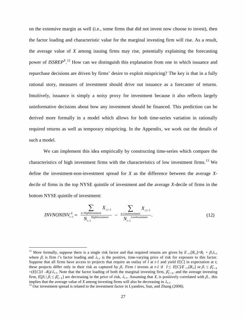
on the extensive margin as well (i.e., some firms that did not invest now choose to invest), then

the factor loading and characteristic value for the marginal investing firm will rise. As a result,

the average value of X among issuing firms may rise, potentially explaining the forecasting

power of ISSREPX.12

We can implement this idea empirically by constructing time-series which compare the

characteristics of high investment firms with the characteristics of low investment firms.

How can we distinguish this explanation from one in which issuance and

repurchase decisions are driven by firms’ desire to exploit mispricing? The key is that in a fully

rational story, measures of investment should drive out issuance as a forecaster of returns.

Intuitively, issuance is simply a noisy proxy for investment because it also reflects largely

uninformative decisions about how any investment should be financed. This prediction can be

derived more formally in a model which allows for both time-series variation in rationally

required returns as well as temporary mispricing. In the Appendix, we work out the details of

such a model.

13

We

define the investment-non-investment spread for X as the difference between the average X-

decile of firms in the top NYSE quintile of investment and the average X-decile of firms in the

bottom NYSE quintile of investment:

, 1 , 1

11 1

.i t i t

i HighInvestmentX i LowInvestmentt HighInvestment LowInvestment

t t

X XINVNONINV

N N

− −∈ ∈

−− −

= −∑ ∑

(12)

12 More formally, suppose there is a single risk factor and that required returns are given by E t-1[Ri,t]=Rf + βiλt-1 where βi is firm i’s factor loading and λt-1 is the positive, time-varying price of risk for exposure to this factor. Suppose that all firms have access to projects that require an outlay of I at t-1 and yield E[C] in expectation at t; these projects differ only in their risk as captured by βi. Firm i invests at t-1 if I ≤ E[C]/E t-1[Ri,t] or βi ≤ =(E[C]/I –Rf)/λt-1. Note that the factor loading of both the marginal investing firm, , and the average investing firm, E[βi | βi ≤ ] are decreasing in the price of risk, λt-1. Assuming that Xi is positively correlated with βi , this implies that the average value of X among investing firms will also be decreasing in λt-1. 13 Our investment spread is related to the investment factor in Lyandres, Sun, and Zhang (2008).

28

For example, 1 1MEtINVNONINV − = indicates that high investment firms were on average

one size decile larger than low investment firms in year t-1. To measure investment in equation

(14), we use capital expenditures over assets (CAPX/A). We also construct INVNONINV using

debt growth. Investment can be funded using either debt, equity, or internal funds, but

mispricing-related explanations would have firms favor equity over debt when equity was

perceived to be overvalued. Thus, debt growth can be interpreted as residual investment after

netting out the portion that is funded by equity.14

Table 8 summarizes the INVNONINVX variables, as well as describing their correlations

with the corresponding characteristic issuer-repurchaser spreads. As expected, the table shows

that INVNONINVX is generally positively correlated with ISSREPX, with an average correlation

of 0.32 in Panel A and 0.21 in Panel B. There are some exceptions, however. For instance, the

correlation between the investment based spread and ISSREPX actually turns negative in Panel A

for the age and distress attributes.

In Table 9 we use the investment-noninvestment spread to forecast returns to

characteristic portfolios:

1X X

t t tR a c INVNONINV u−= + ⋅ + (13)

Panel A shows these results when investment is measured using capital expenditures; in Panel B

investment is the percentage growth in debt. As can be seen in the table, the results are mixed.

For the full 1963-2007 sample period, only nominal share price is significant in both Panels A

and B, while profitability (E/B) is also significant when investment is measured using debt

growth. And, for six of the eleven characteristics, the sign goes the wrong direction when

investment is measured using CAPX/A. The results are slightly stronger in the 1973-2007 period.

14 A related construction is to use asset growth as a measure of investment. This combines equity and debt funded investment. These results are shown in the Internet Appendix.

29

For instance, the coefficient for size is now significant in Panel A and is marginally significant in

Panel B. Overall, these investment-based measures have some modest ability to forecast

characteristic-level returns.

In Table 10, we run a horse-race between INVNONINVX and our ISSREPX variable to

forecast future characteristic returns:

1 1X X X

t t t tR a b ISSREP c INVNONINV u− −= + ⋅ + ⋅ + (14)

Recall that under the null hypothesis where all time-variation in expected returns is due to

variation in rationally required returns, ISSREPX is simply a noisy proxy for INVNONINVX. We

consider first the results in Panel A, where investment is measured as capital expenditures. For

nearly every characteristic, the coefficient b on ISSREPX is nearly identical to its value in the

univariate regressions shown in Table 4. For example, for the 1963-2007 sample period, b=-

0.713 for book-to-market and -0.214 for size in Table 4, and -0.734 and -0.229 in Table 10.

Interestingly, the coefficient c on INVNONINVX is no longer significant for a single

characteristic, and the vast majority of the time goes in the wrong direction. This same general

pattern emerges in Panel B where investment is measured as the percentage change in debt.

While c is statistically significant for sales growth in the 1963-2007 period and for share price

and profitability in the 1973-2007 period, the coefficients on ISSREPX are again largely

unaffected in Panel B. In summary, explanations based on time-varying risk premia – at least

insofar as they should drive firm-level investment – do not fare well in our forecasting

regressions.

One potential objection is that these rational explanations link required returns to

investment plans, but there may be a short gap between investment plans and realized investment

(e.g., Lamont (2000)). In this case, one could argue that issuance is perhaps a better proxy for

30

investment plans than investment itself. While we cannot rule out this explanation entirely, we

can look ahead to firms’ future investment rates. Specifically, we can construct INVNOINVX

based on future capital expenditures, and run the same horse race as shown in Table 10. These

results are similar (see Internet Appendix) in that the coefficients on ISSREPX are virtually

unchanged compared to the univariate specifications in Table 4. Another robustness test is

construct INVNOINVX based on asset growth (conceptually we prefer measures based on capital

expenditures or debt growth because asset growth combines growth in both financial and real

assets, and thus is mechanically linked to equity issues). In the Internet Appendix, we show

results for this alternate construction as well, reaching similar conclusions.

Taken together, it is difficult to fully explain our results within a straightforward rational

framework. At the same time, our results do not show that all time variation in expected

characteristic returns is due to mispricing. However, they do lend support to the view that public

companies have successfully timed characteristic returns in their issuance and repurchase

decisions.

VI. Evaluating the importance of characteristic timing for corporate issuance

The previous section suggests that issuance and repurchase activity is partly an attempt to

exploit time-varying characteristic mispricing. But what fraction of the underperformance of net

issuers does such characteristic timing explain? We can address this question by modifying the

approach in Daniel, Grinblatt, Titman, and Wermers (1997). Specifically, we decompose the

return to a long-short strategy based on net stock issuance into three components: the return in

excess of the return on firms with similar characteristics (“characteristic selectivity”), the return

associated with the long-run average characteristics of the net issuance portfolio (“average

31

style”), and the return associated with the timing of those characteristics (“characteristic

timing”).

Each year we form a portfolio that is long (short) firms in the lowest (highest) NYSE

decile of net stock issuance. Motivated by our earlier findings, we limit our matching

characteristics to size and book-to-market, so the results should be seen as a lower bound

estimate of the importance of characteristic timing. We match each firm in this portfolio to one

of 25 size and book-to-market benchmark portfolios. To construct these benchmarks, firms are

first grouped by NYSE size quintile, and within each size quintile, we then sort firms into book-

to-market quintiles. The benchmark portfolios include only seasoned firms that did not issue or

repurchase stock in the prior year.

Following Daniel, Grinblatt, Titman, and Wermers (1997), characteristic selectivity is the

difference between the portfolio return and the weighted return on the matched benchmark

portfolios. Next, let , 1b tw − denote the total portfolio weight of firms matched to benchmark b at

time t-1. The average style and characteristic timing components of the net issuance portfolio

return are

t bbtb

AS w R= ∑ , and (15)

, 1( ) bt bb t b tC wwT R− −= ∑ . (16)

where bw denotes the time-series mean of bw . The average style term reflects the performance on

a benchmark portfolio that captures the average size and B/M composition of the NS portfolio.

The characteristic timing component reflects deviations of the current size and B/M composition

of the portfolio from its long-run average.15

15 Our measure captures the ability of issuers to time characteristics at both short and long horizons whereas the measure used in the mutual fund literature is primarily designed to capture timing ability at shorter horizons.

32

We report the results of this decomposition in Table 11. Each row decomposes the return

on the net stock issuance portfolio into CS, AS, and CT components. We show results for both

value and equal-weighted portfolios based on NS. The first column shows the average return to

the long-short NS strategy. For the value-weighted NS strategy, the 9.23% annual return can be

decomposed into a 7.39% characteristic selectivity return, an -0.08% average style return, and a

1.92% characteristic timing return. Thus, approximately 21 percent of the forecasting ability of

NS in the cross-section comes from firms’ ability to time size and book-to-market characteristics.

The results for the equal- and value-weighted portfolios are similar.

VII. Conclusion

Firms are well suited to time broad patterns of characteristic-based mispricing. When

investors demand a particular characteristic, firms absorb some of that demand by issuing new

equity. When a particular characteristic is out of favor, firms endowed with that characteristic

repurchase shares. Consistent with this idea, time-series variation in the differences between the

attributes of stock issuers and repurchasers forecasts characteristic-related stock returns. Our

approach helps forecast returns to portfolios based on book-to-market, size, share price, distress,

payout policy, profitability, and industry.

Our work has implications for the large literature that studies the stock market

performance of SEOs, IPOs, and recent acquirers. In many of these studies, researchers purge the

returns of event firms of size and book-to-market effects. Our findings suggest that this

methodology is too conservative, since, for example, low market-to-book firms issue stock just

prior to periods when low market-to-book firms in general are going to perform poorly. More

broadly, event studies that compare the performance of sample firms to firms matched on

33

characteristics will omit any returns coming from event firms’ ability to time those

characteristics.

Although characteristic timing based on size and book-to-market only explains a modest

portion of the total underperformance of issuers, it is interesting to contrast this with studies of

mutual fund performance (i.e. Grinblatt, Titman, and Wermers (1997) and Wermers (2000)).

These studies typically find that mutual funds have very small or even slightly negative

characteristic timing ability. The contrast between these studies and our findings for issuing

firms is consistent with the view that corporations may have a comparative advantage over

professional investors in attacking certain forms of broad-based mispricing. This advantage may

be greatest when mispricing converges slowly or is associated with undiversifiable risk. It is

plausible that these conditions could be satisfied for the most salient characteristics we consider,

including size, book-to-market, and industry.

34

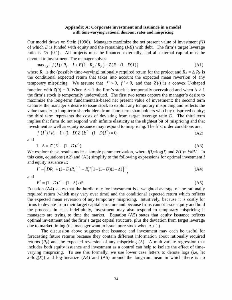
Appendix A: Corporate investment and issuance in a model with time-varying rational discount rates and mispricing

Our model draws on Stein (1996). Managers maximize the net present value of investment f(I) of which E is funded with equity and the remaining (I-E) with debt. The firm’s target leverage ratio is (0,1)D ∈ . All projects must be financed externally, and all external capital must be devoted to investment. The manager solves:

( ){ },max ( ) / 1 / ( (1 ) )I E F Ff I R I E R R Z E D I∆− + − − − − (A1) where RF is the (possibly time-varying) rationally required return for the project and R∆ = ∆ RF is the conditional expected return that takes into account the expected mean reversion of any temporary mispricing. We assume that ' 0, '' 0,f f> < and that ( )Z ⋅ is a convex U-shaped function with Z(0) = 0. When ∆ < 1 the firm’s stock is temporarily overvalued and when ∆ > 1 the firm’s stock is temporarily undervalued. The first two terms capture the manager’s desire to maximize the long-term fundamentals-based net present value of investment; the second term captures the manager’s desire to issue stock to exploit any temporary mispricing and reflects the value transfer to long-term shareholders from short-term shareholders who buy mispriced equity; the third term represents the costs of deviating from target leverage ratio D. The third term implies that firms do not respond with infinite elasticity at the slightest bit of mispricing and that investment as well as equity issuance may respond to mispricing. The first order conditions are:

* * *( ) / 1 (1 ) ( (1 ) ) 0,Ff I R D Z E D I′ ′− + − − − = (A2) and

* *1 ( (1 ) ).Z E D I′− ∆ = − − (A3) We explore these results under a simple parameterization, where f(I)=log(I) and Z(L)= ½θL2. In this case, equations (A2) and (A3) simplify to the following expressions for optimal investment I and equity issuance E:

[ ] [ ]1 1* 1(1 ) 1 (1 )(1 )F FI DR D R R D− −−∆= + − = − − − ∆ , (A4)

and * *(1 ) (1 ) / .E D I θ= − + − ∆ (A5)

Equation (A4) states that the hurdle rate for investment is a weighted average of the rationally required return (which may vary over time) and the conditional expected return which reflects the expected mean reversion of any temporary mispricing. Intuitively, because it is costly for firms to deviate from their target capital structure and because firms cannot issue equity and hold the proceeds in cash indefinitely, investment may also respond to temporary mispricing if managers are trying to time the market. Equation (A5) states that equity issuance reflects optimal investment and the firm’s target capital structure, plus the deviation from target leverage due to market timing (the manager want to issue more stock when ∆ < 1). The discussion above suggests that issuance and investment may each be useful for forecasting future returns because they contain different information about rationally required returns (RF) and the expected reversion of any mispricing (∆). A multivariate regression that includes both equity issuance and investment as a control can help to isolate the effect of time-varying mispricing. To see this formally, we use lower case letters to denote logs (i.e, let x=log(X)) and log-linearize (A4) and (A5) around the long-run mean in which there is no

35

mispricing (∆=1) and rationally required returns are R . This yields the following expressions for log investment and equity issuance at time t:

* *,( ) (1 ) ,t F t ti i r r D δ− = − − − − (A6)

and * * * *

, (1 )(1 ) (

( ) ( )1

.)t F t t t t t

Re e r r i i RDD D

δ δ δθ θ

− = − − − − −− −

− = − (A7)

Consider the following thought experiment, in which we compare the effect of changes in the rational discount rate (rF,t) on it

*and et*, with the effect of changes in expected returns due to

mispricing (δt). Reductions in rF,t increase both investment and equity issuance one-for-one. Reductions in δt increase investment, but less so than reductions in rF,t. This is because managers trade off the benefits of market timing against the costs of overinvestment. The above expressions also show that et

* will respond more elastically than it* to changes in δt. Moreover,

assuming that / ( (1 ))R D Dθ < − so that the costs of deviating from target leverage are not too high, issuance will respond more to a given change in δt than a comparable change in rF,t.

Now suppose that the realized log return at time t+1 is given by rt+1 =rF,t + δt + εt+1 and assume that the three terms are uncorrelated. We first consider the case in which there is time series variation in both rF,t and δt. Now, the coefficient on et

* in a univariate return forecasting regression is given by:

*,1

* 2,

[ ] [(1 ) ( / ((1 ) ))] [ ][ , ] .[ ] [ ] [(1 ) ( / ((1 ) ))] [ ]

F t tt tu

t F t t

Var r D R D VarCov e rbVar e Var r D R D Var

θ δθ δ

+ + − + − ⋅= = −

+ − + − ⋅ (A8)

Similarly, the coefficient on it* in a univariate return forecasting regression is given by:

*,1

* 2,

[ ] (1 ) [ ][ , ] .[ ] [ ] (1 ) [ ]

F t tt tu

t F t t

Var r D VarCov i rVar i Var r D Var

cδδ

+ + − ⋅= = −

+ − ⋅ (A9)

By contrast in a multivariate regression, we have: 1* * * *

1* * * *

1

(1 )( ) /[ ] [ , ] [ , ]( ) /[ , ] [ ] ]

., 1 (1[ )

m t t t t t

t t t tm t

D D RVar e Cov e i Cov e rD RCov e i Var i Cov i r

bc D

θθ

+

+

−

= = − + −

−

−

(A10)

Again, assuming that / ( (1 ))R D Dθ < − , it follows that 1 0u mb b− < < < and 1 0u mc c< − < < . That is, the coefficients on equity issuance and investment from a multivariate regression that includes both variables will be smaller in magnitude than the corresponding univariate coefficients due to a classic omitted variable bias. However, in a fully rational model with Var[δt] = 0 or in the absence of managerial attempts to time mispricing, one would expect investment to drive out issuance in a multivariate specification as long as there is some amount of noise in financing decisions. (In the absence of any noise, investment and issuance would be perfectly collinear in this case.) One way to model this noise is to assume that target leverage ratios fluctuate in ways that are uncorrelated with expected returns. Under this assumption, (A6) remains unchanged and (A7) becomes:

* * * *

(1 ) (1( ( )

)) ,t t t t

R DD

e e i i d dD

δθ

−− −

− = − − − (A11)

where td d− represents the deviation of target leverage from its long-run mean. The intuition is that changes in target leverage have a first order effect on equity issuance, but only affect

36

investment when 1∆ ≠ . In this case, the coefficient on investment from a univariate forecasting regression (cu) remains unchanged, the coefficient on issuance (bu) in a univariate regression is:

,2 2

,

[ ] [(1 ) ( / ((1 ) ))] [ ],

[ ] [(1 ) ( / ((1 ) ))] [ ] ( / (1 )) [ ]F t t

uF t t t

Var r D R D Varb

Var r D R D Var D D Var dθ δ

θ δ+ − + − ⋅

−+ − + − ⋅ + − ⋅

=

(A12)

and a multivariate regression yields:

2 2 2 2

2 2 2

2 2 2

,

, ,

, ,

, ,

[ ] [ ] (1- )[ ] [ ]+ [ ] [ [ ] (1 ) [ ]]

[ ] [ ] [ (1- )] [ ] [ [ ] (1 ) [ ]][ ] [ ]+ [ ] [ [

F t

F t F t

F t

t

t t tm

m t t t

t t

F t

F t F t

Var Var R D DR Var Var Var d D Var D Varb

c Var Var R R D D Var d D Var D VarR Var Va

rr r

r rr Var d D Vr rar

δ θδ θ δ

δ θ θ δδ θ

⋅⋅ + −

= − ⋅ − + ⋅ + − ⋅ 2

.

] (1 ) [ ]]t tD Var δ

+ −

(A13)

(A13) reduces to (A10) when Var[dt] = 0. It is straightforward to see from (A13) that so long as Var[dt] > 0 investment will completely drive out issuance in a horse race when Var[rF,t] = 0 or Var[δt] = 0. The same result obtains if managers do not issue equity to exploit mispricing. The intuition is that in each case, equity issuance contains no additional information about expected returns over and above investment. Thus, it is driven out in a horse race because it also reflects a series of uninformative decisions about how investment should be financed.

37

Appendix B: Characteristic Definitions

Where applicable, we provide in parentheses the relevant Compustat data items from the Fundamentals Annual file. When matching to returns in July of year t to June of t+1, we follow the Fama and French (1992) convention that accounting variables are measured as of fiscal year ending t-1, and market-based variables (ME, P, β, σ, as well as the market-based components of SHUM) are measured as of June of year t. However, we label all of these characteristics as year t-1 for notational convenience.

Book-to-market equity (B/M): Book equity is stockholder's equity, plus balance sheet deferred taxes (item TXDB) and investment tax credits (ITCB) each when available, minus preferred stock. For stockholder’s equity we use item SEQ when available; if SEQ is missing we use the book value of common equity (CEQ) plus the book value of preferred stock (PSTK); finally, we use total assets (AT) minus total liabilities (LT) minus minority interest (MIB). For preferred stock we use redemption value (PSTKRV), liquidation value (PSTKL), and book value (PSTK) in that order. We divide book equity for fiscal years ending in year t-1 by the value of market equity at the end of December in year t-1 from CRSP. Sales Growth (ΔS t/S t-1): Sales growth is the log change in sales (SALE).

Accruals (Acc/A): Following Bergstresser and Philippon (2006) we define accruals as

1

( ) ( )( / ) .( / 2)

t t t t t tt

t t

CurrAssets Cash CurrLiab STDebt TaxesPayable DeprecAcc AA A −

∆ − ∆ − ∆ − ∆ − ∆ −=

+

where current assets is Compustat item ACT, cash is item CHE, current liabilities is item LCT, taxes payable is item TXP, and depreciation is item DP.

Size: Size is market equity (ME) at the end of June in year t. Price: Price is the nominal price per share at the end of June in year t. Age: Age is number of years since the first appearance of a firm (PERMCO) on CRSP measured to the nearest month.

Beta (β) and Volatility (σ): Beta and volatility are estimated from a trailing 24-month CAPM regression. We require that a firm has valid returns for at least 12 of the previous 24 months.

Distress (SHUM): We use the bankruptcy hazard rate estimated by Shumway (2001): exp( ) / (1 exp( ))SHUM H H= − where

0.461 73.303 1.982 / 3.59 1.809 ( ) 53 7/ . 91MH NI A L A RELSIZE R R σ= − − ⋅ + ⋅ ⋅ − +⋅− ⋅− NI/A is net income over period-end assets, L/A is total liabilities over assets, RELSIZE is the log of a firm's market equity divided by the total capitalization of all NYSE and AMEX stocks,

MR R− is firm's cumulative return over the prior 12-months minus the cumulative return on the value-weighted NYSE/AMEX index, and σ is volatility of residuals from trailing 12-month market-model regression.

Dividends (Div): Div is a dummy variable equal to one for dividend payers (firms for which DVPSXF>0) and zero for nonpayers.

Profitability (E/B): Earnings (E) is income before extraordinary available for common (IBCOM) plus income statement deferred taxes (TXDI) when available. Income is scaled by average book equity where book equity is as defined above.

38

References

Amihud, Yakov, and Clifford M. Hurvich, 2004, Predictive regressions: A reduced-bias estimation method, Journal of Financial and Quantitative Analysis 39, 813-841.

Bagwell, Laurie Simon, and John B. Shoven, 1989, Cash distributions to shareholders, Journal of Economic Perspectives, 129-140.

Baker, Malcolm, Richard Ruback, and Jeffrey Wurgler, 2007, Behavioral Corporate Finance: A Survey, in Espen Eckbo, ed, Handbook of Corporate Finance: Empirical Corporate Finance.

Baker, Malcolm, Ryan Taliaferro, and Jeffrey Wurgler, 2006, Predicting returns with managerial decision variables: Is there a small-sample bias?, Journal of Finance 61, 1711-1730.

Baker, Malcolm, and Jeffrey Wurgler, 2000, The equity share in new issues and aggregate stock returns, Journal of Finance 55, 2219 – 2257.

Baker, Malcolm, and Jeffrey Wurgler, 2004, A catering theory of dividends, Journal of Finance,1125-1165.

Baker, Malcolm, and Jeffrey Wurgler, 2006, Investor sentiment and the cross-section of stock returns, Journal of Finance 61, 1645-1680.

Barberis, Nicholas and Andrei Shleifer, 2003, Style investing, Journal of Financial Economics 68, 161 – 199.

Benartzi, Shlomo, Roni Michaely, Richard Thaler, and William Weld, 2007, The nominal price puzzle, Working paper.

Bergstresser, Daniel, and Thomas Philippon, 2006, CEO incentives and earnings management, Journal of Financial Economics, 511-529.

Butler Alex, Gustavo Grullon, and James Weston, 2005, Journal of Finance 60, 963 – 986.

Carlson, Murray, Adlai Fisher, and Ron Giammarino, 2006, Corporate Investment and Asset Price Dynamics: Implications for SEO Event Studies and Long-Run Performance, Journal of Finance 61, 1009 – 1034.

Chan, Louis K, Josef Lakonishok, and Bhaskaran Swaminathan, 2007, Industry classifications and return comovement, Financial Analysts Journal 63, 56-71.

Cohen, Randolph, Samuel Thompson, and Tuomo Vuolteenaho, 2006, Cross-sectional forecasts of the equity premium, Journal of Financial Economics 81, 101-141.

Daniel, Kent and Sheridan Titman, 1997, Evidence on the characteristics of cross-sectional variation in stock returns, Journal of Finance 52, 1 – 33.

39

Daniel, Kent, Mark Grinblatt, Sheridan Titman, and Russ Wermers, 1997, Measuring mutual fund performance with characteristic based benchmarks, Journal of Finance 52, 1035-1038.

Eckbo, Espen, Ronald Masulis, and Oyvind Norli, 2000, Seasoned public offerings: Resolution of the new issues puzzle, Journal of Financial Economics 56, 251-291.

Fama, Eugene F. and Kenneth R. French, 1992, The cross-section of expected stock returns, Journal of Finance 47, 427-465.

Fama, Eugene F. and Kenneth R. French, 1993, Common risk factors in the returns on stocks and bonds, Journal of Financial Economics 33, 3-56.

Fama, Eugene F. and Kenneth R. French, 1997, Industry costs of equity, Journal of Financial Economics 43, 153-193.

Fama, Eugene F. and Kenneth R. French, 2004, New lists: fundamentals and survival rates, Journal of Financial Economics 72, 229 – 269.

Fama, Eugene F. and Kenneth R. French, 2005, Financing decisions: who issues stock?, Journal of Financial Economics, 76, 549 – 582.

Fama, Eugene F. and Kenneth R. French, 2008a, Dissecting anomalies, Journal of Finance 63, 1653-1678.

Fama, Eugene F. and Kenneth R. French, 2008b, Average returns, B/M, and share issues, Journal of Finance 63, 2971-2995.

Fama, Eugene F. and Kenneth R. French, 2008c, Opportunistic financing, Working paper.

Fama, Eugene F. and James Macbeth, 1973, Risk, return, and equilibrium: Empirical tests, Journal of Political Economy 81, 607-636.

Graham, Benjamin, 1973, The Intelligent Investor, 4th ed., Harper & Row.

Graham, John R., and Campbell R. Harvey, 2001, The theory and practice of corporate finance: evidence from the field, Journal of Financial Economics 60, 187-243.

Daniel, Kent, Mark Grinblatt, Sheridan Titman, and Russ Wermers, 1997, Measuring mutual fund performance with characteristics-based benchmarks, Journal of Finance 52, 1035-1058.Carlson, Murray, Adlai Fisher, and Ron Giammarino, 2004, Corporate investment and asset price dynamics: Implications for the cross-section of returns, Journal of Finance 59, 2577-2603.

Carlson, Murray, Adlai Fisher, and Ron Giammarino, 2006, Corporate investment and asset price dynamics: Implications for SEO event studies and long-run performance, Journal of Finance 61, 1009-1034.

40

Greenwood, Robin, Samuel Hanson, and Jeremy C. Stein, 2010, A gap-filling theory of corporate debt maturity choice, forthcoming Journal of Finance.

Greene, T. Clifton, and Byoung-Hyoun Huang, 2009, Price-based return comovement, Journal of Financial Economics 93, 37-50.

Ikenberry, David, Josef Lakonishok, and Theo Vermaelen, 1995, Market underreaction to open market share repurchases, Journal of Financial Economics 39, 181 – 208.

Lamont, Owen, 2000, Investment plans and stock returns, Journal of Finance 55, 2719-2745.

Loughran, Tim, and Jay R. Ritter, 1995, The new issues puzzle, Journal of Finance 50, 23 – 51.

Loughran, Tim, and Jay R. Ritter, 2000, Uniformly least powerful tests of market efficiency, Journal of Financial Economics 55, 361-389.

Loughran, Tim, and Jay R. Ritter, 2004, Why has IPO underpricing changed over time?, Financial Management, 5-37.

Louhgran, Tim, and Anand M. Vijh, 1997, Do long-term shareholders benefit from corporate acquisitions? Journal of Finance 52, 1765-1790.

Lyandres, Evgeny, Le Sun, and Lu Zhang, 2008, The new issues puzzle: Testing the investment-based explanation, Review of Financial Studies 21, 2825-2855.

Modigliani, Franco, and Merton H. Miller, 1958, The cost of capital, corporation finance, and the theory of investment, American Economic Review 48, 655–669.

Pontiff, Jeffrey, and Artemiza Woodgate, 2008, Share issuance and cross-sectional returns, Journal of Finance 63, 921 – 945.

Schultz, Paul, 2003, Pseudo Market Timing and the Long-Run Underperformance of IPOs, Journal of Finance 58, 483–517.

Shumway, Tyler, 2001, Forecasting Bankruptcy More Accurately: A Simple Hazard Model, Journal of Business 74, 101-124.

Shleifer, Andrei, and Robert Vishny, 1997, The limits of arbitrage, Journal of Finance 35-55.

Stambaugh, Robert F., 1999, Predictive regressions, Journal of Financial Economics 54, 375-421.

Stein, Jeremy C., 1996, Rational capital budgeting in an irrational world, Journal of Business 69, 429 – 455.

Stein, Jeremy C., 2005, Why Are Most Funds Open-End? Competition and the Limits of Arbitrage, Quarterly Journal of Economics 120, 247-272.

41

Teo, Melvyn and Sung-Jun Woo, 2004. Style effects in the cross-section of stock returns, Journal of Financial Economics 74, 367-398.

Thompson, Samuel, 2006. Simple Formulas for Standard Errors That Cluster by Both Firm and Time. Working paper, Harvard University.

Wermers, Russ, 2000. Mutual fund performance: An empirical decomposition into stock-picking talent, style, transactions costs, and expenses, Journal of Finance 55, 1655-1695.

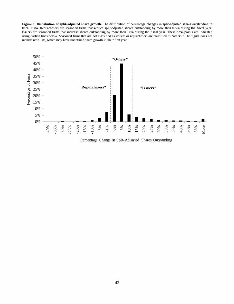
42

Figure 1. Distribution of split-adjusted share growth. The distribution of percentage changes in split-adjusted shares outstanding in fiscal 1984. Repurchasers are seasoned firms that reduce split-adjusted shares outstanding by more than 0.5% during the fiscal year. Issuers are seasoned firms that increase shares outstanding by more than 10% during the fiscal year. These breakpoints are indicated using dashed lines below. Seasoned firms that are not classified as issuers or repurchasers are classified as “others.” The figure does not include new lists, which may have undefined share growth in their first year.

0%5%

10%15%20%25%30%35%40%45%50%

-40%

-35%

-30%

-25%

-20%

-15%

-10% -5%

-1% 0% 5% 10%

15%

20%

25%

30%

35%

40%

45%

50%

55%

Mor

e

Perc

enta

ge o

f Firm

s

Percentage Change in Split-Adjusted Shares Outstanding

"Repurchasers" "Issuers"

"Others"

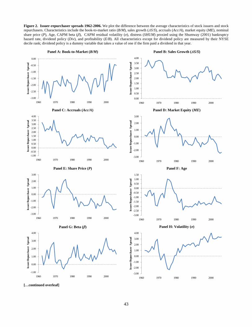
43

Figure 2. Issuer-repurchaser spreads 1962-2006. We plot the difference between the average characteristics of stock issuers and stock repurchasers. Characteristics include the book-to-market ratio (B/M), sales growth (ΔS/S), accruals (Acc/A), market equity (ME), nominal share price (P), Age, CAPM beta (β), CAPM residual volatility (σ), distress (SHUM) proxied using the Shumway (2001) bankruptcy hazard rate, dividend policy (Div), and profitability (E/B). All characteristics except for dividend policy are measured by their NYSE decile rank; dividend policy is a dummy variable that takes a value of one if the firm paid a dividend in that year.

Panel A: Book-to-Market (B/M) Panel B: Sales Growth (ΔS/S)

Panel C: Accruals (Acc/A) Panel D: Market Equity (ME)

Panel E: Share Price (P) Panel F: Age

Panel G: Beta (β) Panel H: Volatility (σ)

[…continued overleaf]

-3.00

-2.50

-2.00

-1.50

-1.00

-0.50

0.00

1960 1970 1980 1990 2000

Issu

er R

epur

chas

er S

prea

d

0.00

0.50

1.00

1.50

2.00

2.50

3.00

3.50

4.00

1960 1970 1980 1990 2000

Issu

er R

epur

chas

er S

prea

d

-1.00-0.500.000.501.001.502.002.503.003.504.00

1960 1970 1980 1990 2000

Issu

er R

epur

chas

er S

prea

d

-3.00

-2.00

-1.00

0.00

1.00

2.00

3.00

1960 1970 1980 1990 2000

Issu

er R

epur

chas

er S

prea

d

-3.00

-2.00

-1.00

0.00

1.00

2.00

3.00

1960 1970 1980 1990 2000

Issu

er R

epur

chas

er S

prea

d

-3.00-2.50-2.00-1.50-1.00-0.500.000.501.001.50

1960 1970 1980 1990 2000

Issu

er R

epur

chas

er S

prea

d

-1.00

0.00

1.00

2.00

3.00

4.00

1960 1970 1980 1990 2000

Issu

er R

epur

chas

er S

prea

d

-3.00

-2.00

-1.00

0.00

1.00

2.00

3.00

4.00

1960 1970 1980 1990 2000

Issu

er R

epur

chas

er S

prea

d

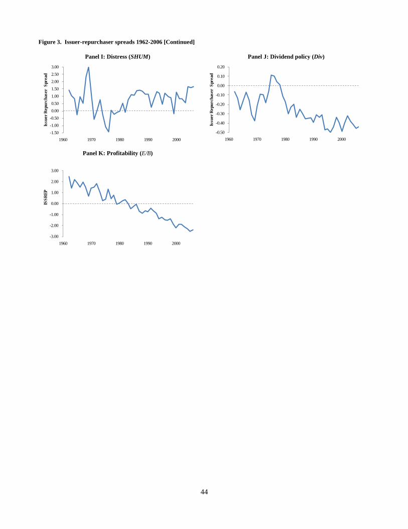
44

Figure 3. Issuer-repurchaser spreads 1962-2006 [Continued]

Panel I: Distress (SHUM) Panel J: Dividend policy (Div)

Panel K: Profitability (E/B)

-1.50-1.00-0.500.000.501.001.502.002.503.00

1960 1970 1980 1990 2000

Issu

er R

epur

chas

er S

prea

d

-0.50

-0.40

-0.30

-0.20

-0.10

0.00

0.10

0.20

1960 1970 1980 1990 2000

Issu

er R

epur

chas

er S

prea

d

-3.00

-2.00

-1.00

0.00

1.00

2.00

3.00

1960 1970 1980 1990 2000

ISSR

EP

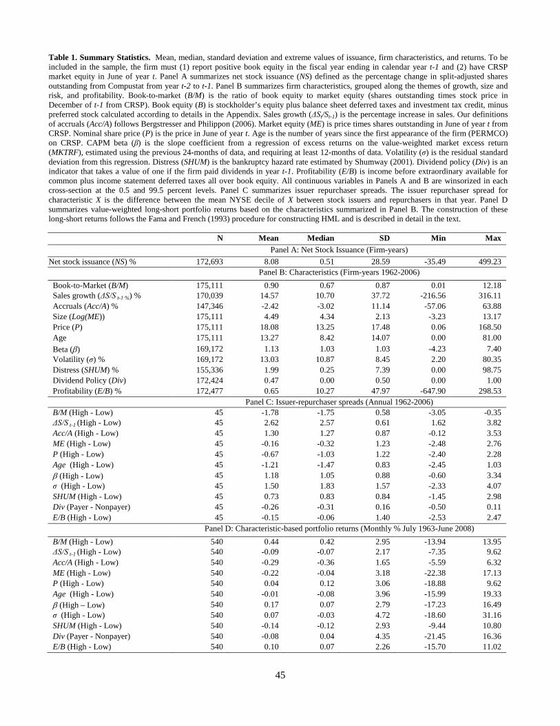
45

Table 1. Summary Statistics. Mean, median, standard deviation and extreme values of issuance, firm characteristics, and returns. To be included in the sample, the firm must (1) report positive book equity in the fiscal year ending in calendar year t-1 and (2) have CRSP market equity in June of year t. Panel A summarizes net stock issuance (NS) defined as the percentage change in split-adjusted shares outstanding from Compustat from year t-2 to t-1. Panel B summarizes firm characteristics, grouped along the themes of growth, size and risk, and profitability. Book-to-market (B/M) is the ratio of book equity to market equity (shares outstanding times stock price in December of t-1 from CRSP). Book equity (B) is stockholder’s equity plus balance sheet deferred taxes and investment tax credit, minus preferred stock calculated according to details in the Appendix. Sales growth (ΔSt/St-1) is the percentage increase in sales. Our definitions of accruals (Acc/A) follows Bergstresser and Philippon (2006). Market equity (ME) is price times shares outstanding in June of year t from CRSP. Nominal share price (P) is the price in June of year t. Age is the number of years since the first appearance of the firm (PERMCO) on CRSP. CAPM beta (β) is the slope coefficient from a regression of excess returns on the value-weighted market excess return (MKTRF), estimated using the previous 24-months of data, and requiring at least 12-months of data. Volatility (σ) is the residual standard deviation from this regression. Distress (SHUM) is the bankruptcy hazard rate estimated by Shumway (2001). Dividend policy (Div) is an indicator that takes a value of one if the firm paid dividends in year t-1. Profitability (E/B) is income before extraordinary available for common plus income statement deferred taxes all over book equity. All continuous variables in Panels A and B are winsorized in each cross-section at the 0.5 and 99.5 percent levels. Panel C summarizes issuer repurchaser spreads. The issuer repurchaser spread for characteristic X is the difference between the mean NYSE decile of X between stock issuers and repurchasers in that year. Panel D summarizes value-weighted long-short portfolio returns based on the characteristics summarized in Panel B. The construction of these long-short returns follows the Fama and French (1993) procedure for constructing HML and is described in detail in the text.

N Mean Median SD Min Max Panel A: Net Stock Issuance (Firm-years) Net stock issuance (NS) % 172,693 8.08 0.51 28.59 -35.49 499.23 Panel B: Characteristics (Firm-years 1962-2006)

Book-to-Market (B/M) 175,111 0.90 0.67 0.87 0.01 12.18 Sales growth (ΔS/S t-1 %) % 170,039 14.57 10.70 37.72 -216.56 316.11 Accruals (Acc/A) % 147,346 -2.42 -3.02 11.14 -57.06 63.88 Size (Log(ME)) 175,111 4.49 4.34 2.13 -3.23 13.17 Price (P) 175,111 18.08 13.25 17.48 0.06 168.50 Age 175,111 13.27 8.42 14.07 0.00 81.00 Beta (β) 169,172 1.13 1.03 1.03 -4.23 7.40 Volatility (σ) % 169,172 13.03 10.87 8.45 2.20 80.35 Distress (SHUM) % 155,336 1.99 0.25 7.39 0.00 98.75 Dividend Policy (Div) 172,424 0.47 0.00 0.50 0.00 1.00 Profitability (E/B) % 172,477 0.65 10.27 47.97 -647.90 298.53 Panel C: Issuer-repurchaser spreads (Annual 1962-2006) B/M (High - Low) 45 -1.78 -1.75 0.58 -3.05 -0.35 ΔS/S t-1 (High - Low) 45 2.62 2.57 0.61 1.62 3.82 Acc/A (High - Low) 45 1.30 1.27 0.87 -0.12 3.53 ME (High - Low) 45 -0.16 -0.32 1.23 -2.48 2.76 P (High - Low) 45 -0.67 -1.03 1.22 -2.40 2.28 Age (High - Low) 45 -1.21 -1.47 0.83 -2.45 1.03 β (High - Low) 45 1.18 1.05 0.88 -0.60 3.34 σ (High - Low) 45 1.50 1.83 1.57 -2.33 4.07 SHUM (High - Low) 45 0.73 0.83 0.84 -1.45 2.98 Div (Payer - Nonpayer) 45 -0.26 -0.31 0.16 -0.50 0.11 E/B (High - Low) 45 -0.15 -0.06 1.40 -2.53 2.47

Panel D: Characteristic-based portfolio returns (Monthly % July 1963-June 2008) B/M (High - Low) 540 0.44 0.42 2.95 -13.94 13.95 ΔS/S t-1 (High - Low) 540 -0.09 -0.07 2.17 -7.35 9.62 Acc/A (High - Low) 540 -0.29 -0.36 1.65 -5.59 6.32 ME (High - Low) 540 -0.22 -0.04 3.18 -22.38 17.13 P (High - Low) 540 0.04 0.12 3.06 -18.88 9.62 Age (High - Low) 540 -0.01 -0.08 3.96 -15.99 19.33 β (High – Low) 540 0.17 0.07 2.79 -17.23 16.49 σ (High - Low) 540 0.07 -0.03 4.72 -18.60 31.16 SHUM (High - Low) 540 -0.14 -0.12 2.93 -9.44 10.80 Div (Payer - Nonpayer) 540 -0.08 0.04 4.35 -21.45 16.36 E/B (High - Low) 540 0.10 0.07 2.26 -15.70 11.02

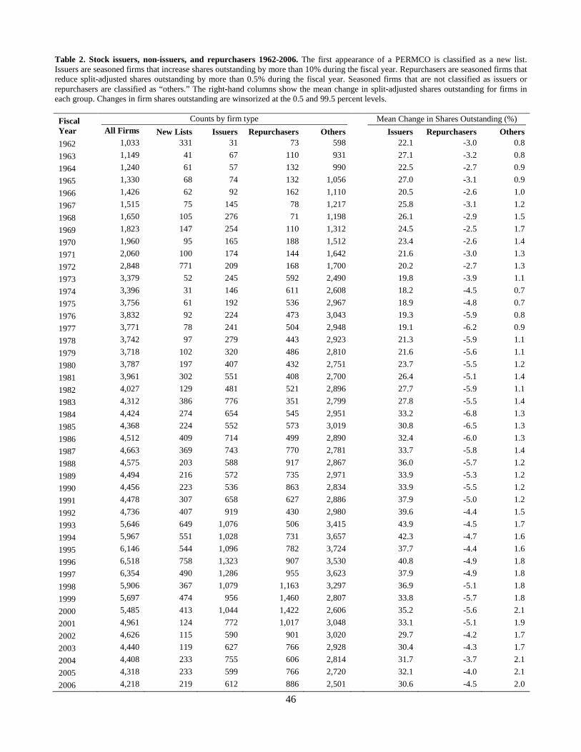
46

Table 2. Stock issuers, non-issuers, and repurchasers 1962-2006. The first appearance of a PERMCO is classified as a new list. Issuers are seasoned firms that increase shares outstanding by more than 10% during the fiscal year. Repurchasers are seasoned firms that reduce split-adjusted shares outstanding by more than 0.5% during the fiscal year. Seasoned firms that are not classified as issuers or repurchasers are classified as “others.” The right-hand columns show the mean change in split-adjusted shares outstanding for firms in each group. Changes in firm shares outstanding are winsorized at the 0.5 and 99.5 percent levels.

Fiscal Year

Counts by firm type Mean Change in Shares Outstanding (%) All Firms New Lists Issuers Repurchasers Others Issuers Repurchasers Others

1962 1,033 331 31 73 598 22.1 -3.0 0.8 1963 1,149 41 67 110 931 27.1 -3.2 0.8 1964 1,240 61 57 132 990 22.5 -2.7 0.9 1965 1,330 68 74 132 1,056 27.0 -3.1 0.9 1966 1,426 62 92 162 1,110 20.5 -2.6 1.0 1967 1,515 75 145 78 1,217 25.8 -3.1 1.2 1968 1,650 105 276 71 1,198 26.1 -2.9 1.5 1969 1,823 147 254 110 1,312 24.5 -2.5 1.7 1970 1,960 95 165 188 1,512 23.4 -2.6 1.4 1971 2,060 100 174 144 1,642 21.6 -3.0 1.3 1972 2,848 771 209 168 1,700 20.2 -2.7 1.3 1973 3,379 52 245 592 2,490 19.8 -3.9 1.1 1974 3,396 31 146 611 2,608 18.2 -4.5 0.7 1975 3,756 61 192 536 2,967 18.9 -4.8 0.7 1976 3,832 92 224 473 3,043 19.3 -5.9 0.8 1977 3,771 78 241 504 2,948 19.1 -6.2 0.9 1978 3,742 97 279 443 2,923 21.3 -5.9 1.1 1979 3,718 102 320 486 2,810 21.6 -5.6 1.1 1980 3,787 197 407 432 2,751 23.7 -5.5 1.2 1981 3,961 302 551 408 2,700 26.4 -5.1 1.4 1982 4,027 129 481 521 2,896 27.7 -5.9 1.1 1983 4,312 386 776 351 2,799 27.8 -5.5 1.4 1984 4,424 274 654 545 2,951 33.2 -6.8 1.3 1985 4,368 224 552 573 3,019 30.8 -6.5 1.3 1986 4,512 409 714 499 2,890 32.4 -6.0 1.3 1987 4,663 369 743 770 2,781 33.7 -5.8 1.4 1988 4,575 203 588 917 2,867 36.0 -5.7 1.2 1989 4,494 216 572 735 2,971 33.9 -5.3 1.2 1990 4,456 223 536 863 2,834 33.9 -5.5 1.2 1991 4,478 307 658 627 2,886 37.9 -5.0 1.2 1992 4,736 407 919 430 2,980 39.6 -4.4 1.5 1993 5,646 649 1,076 506 3,415 43.9 -4.5 1.7 1994 5,967 551 1,028 731 3,657 42.3 -4.7 1.6 1995 6,146 544 1,096 782 3,724 37.7 -4.4 1.6 1996 6,518 758 1,323 907 3,530 40.8 -4.9 1.8 1997 6,354 490 1,286 955 3,623 37.9 -4.9 1.8 1998 5,906 367 1,079 1,163 3,297 36.9 -5.1 1.8 1999 5,697 474 956 1,460 2,807 33.8 -5.7 1.8 2000 5,485 413 1,044 1,422 2,606 35.2 -5.6 2.1 2001 4,961 124 772 1,017 3,048 33.1 -5.1 1.9 2002 4,626 115 590 901 3,020 29.7 -4.2 1.7 2003 4,440 119 627 766 2,928 30.4 -4.3 1.7 2004 4,408 233 755 606 2,814 31.7 -3.7 2.1 2005 4,318 233 599 766 2,720 32.1 -4.0 2.1 2006 4,218 219 612 886 2,501 30.6 -4.5 2.0

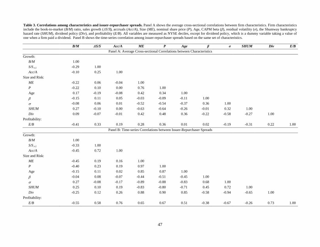
47

Table 3. Correlations among characteristics and issuer-repurchaser spreads. Panel A shows the average cross-sectional correlations between firm characteristics. Firm characteristics include the book-to-market (B/M) ratio, sales growth (ΔS/S), accruals (Acc/A), Size (ME), nominal share price (P), Age, CAPM beta (β), residual volatility (σ), the Shumway bankruptcy hazard rate (SHUM), dividend policy (Div), and profitability (E/B). All variables are measured as NYSE deciles, except for dividend policy, which is a dummy variable taking a value of one when a firm paid a dividend. Panel B shows the time-series correlation among issuer-repurchaser spreads based on the same set of characteristics.

B/M ΔS/S Acc/A ME P Age β σ SHUM Div E/B Panel A: Average Cross-sectional Correlations between Characteristics

Growth: B/M 1.00 S/S t-1 -0.29 1.00 Acc/A -0.10 0.25 1.00

Size and Risk: ME -0.22 0.06 -0.04 1.00 P -0.22 0.10 0.00 0.76 1.00 Age 0.17 -0.19 -0.08 0.42 0.34 1.00 β -0.15 0.11 0.05 -0.03 -0.09 -0.11 1.00 σ -0.08 0.06 0.01 -0.52 -0.54 -0.37 0.36 1.00 SHUM 0.27 -0.10 0.00 -0.63 -0.64 -0.26 -0.01 0.32 1.00 Div 0.09 -0.07 -0.01 0.42 0.48 0.36 -0.22 -0.58 -0.27 1.00

Profitability: E/B -0.41 0.33 0.19 0.28 0.36 0.01 0.02 -0.19 -0.31 0.22 1.00

Panel B: Time-series Correlations between Issuer-Repurchaser Spreads Growth:

B/M 1.00 S/S t-1 -0.33 1.00 Acc/A -0.45 0.72 1.00

Size and Risk: ME -0.45 0.19 0.16 1.00 P -0.40 0.23 0.19 0.97 1.00 Age -0.15 0.11 0.02 0.85 0.87 1.00 β -0.04 0.08 -0.07 -0.44 -0.51 -0.45 1.00 σ 0.27 -0.08 -0.17 -0.89 -0.88 -0.83 0.68 1.00 SHUM 0.25 0.10 0.19 -0.83 -0.80 -0.71 0.45 0.72 1.00 Div -0.25 0.12 0.26 0.88 0.90 0.85 -0.58 -0.94 -0.65 1.00

Profitability: E/B -0.55 0.58 0.76 0.65 0.67 0.51 -0.38 -0.67 -0.26 0.73 1.00

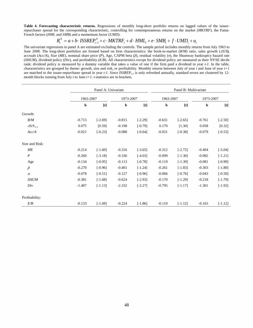
48

Table 4. Forecasting characteristic returns. Regressions of monthly long-short portfolio returns on lagged values of the issuer-repurchaser spread for the corresponding characteristic, controlling for contemporaneous returns on the market (MKTRF), the Fama-French factors (HML and SMB) and a momentum factor (UMD):

1X X

t t t t t t tR a b ISSREP c MKTRF d HML e SMB f UMD u−= + ⋅ + ⋅ + ⋅ + ⋅ + ⋅ +

The univariate regressions in panel A are estimated excluding the controls. The sample period includes monthly returns from July 1963 to June 2008. The long-short portfolios are formed based on firm characteristics: the book-to-market (B/M) ratio, sales growth (ΔS/S), accruals (Acc/A), Size (ME), nominal share price (P), Age, CAPM beta (β), residual volatility (σ), the Shumway bankruptcy hazard rate (SHUM), dividend policy (Div), and profitability (E/B). All characteristics except for dividend policy are measured as their NYSE decile rank; dividend policy is measured by a dummy variable that takes a value of one if the firm paid a dividend in year t-1. In the table, characteristics are grouped by theme: growth, size and risk, or profitability. Monthly returns between July of year t and June of year t+1 are matched to the issuer-repurchaser spread in year t-1. Since ISSREPt-1 is only refreshed annually, standard errors are clustered by 12-month blocks running from July t to June t+1. t-statistics are in brackets.

Panel A: Univariate Panel B: Multivariate

1963-2007 1973-2007 1963-2007 1973-2007 b [t] b [t] b [t] b [t]

Growth: B/M -0.713 [-2.69] -0.815 [-2.29] -0.631 [-2.65] -0.761 [-2.50] ΔS/S t-1 0.075 [0.59] -0.198 [-0.79] 0.170 [1.30] 0.058 [0.32] Acc/A -0.021 [-0.23] -0.088 [-0.64] -0.031 [-0.38] -0.079 [-0.53]

Size and Risk: ME -0.214 [-1.60] -0.316 [-3.65] -0.312 [-2.72] -0.404 [-5.04] P -0.260 [-3.18] -0.336 [-4.03] -0.099 [-1.30] -0.082 [-1.21] Age -0.134 [-0.95] -0.113 [-0.78] -0.119 [-1.39] -0.081 [-0.99]

β -0.270 [-0.96] -0.401 [-1.24] -0.261 [-1.83] -0.303 [-1.80]

σ -0.078 [-0.51] -0.127 [-0.96] -0.066 [-0.76] -0.043 [-0.50] SHUM -0.381 [-1.68] -0.624 [-2.93] -0.170 [-1.29] -0.218 [-1.79] Div -1.407 [-1.13] -2.332 [-2.27] -0.795 [-1.17] -1.301 [-1.92]

Profitability: E/B -0.133 [-1.69] -0.224 [-1.86] -0.110 [-1.12] -0.163 [-1.12]

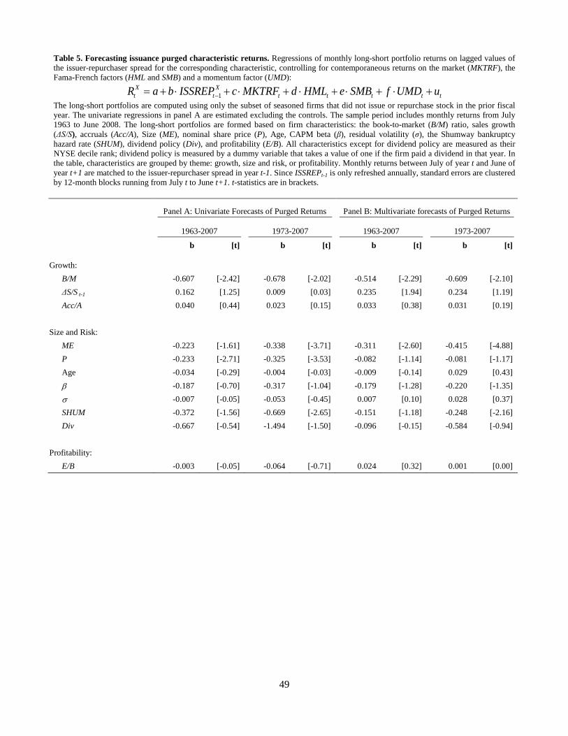
49

Table 5. Forecasting issuance purged characteristic returns. Regressions of monthly long-short portfolio returns on lagged values of the issuer-repurchaser spread for the corresponding characteristic, controlling for contemporaneous returns on the market (MKTRF), the Fama-French factors (HML and SMB) and a momentum factor (UMD):

1X X

t t t t t t tR a b ISSREP c MKTRF d HML e SMB f UMD u−= + ⋅ + ⋅ + ⋅ + ⋅ + ⋅ +

The long-short portfolios are computed using only the subset of seasoned firms that did not issue or repurchase stock in the prior fiscal year. The univariate regressions in panel A are estimated excluding the controls. The sample period includes monthly returns from July 1963 to June 2008. The long-short portfolios are formed based on firm characteristics: the book-to-market (B/M) ratio, sales growth (ΔS/S), accruals (Acc/A), Size (ME), nominal share price (P), Age, CAPM beta (β), residual volatility (σ), the Shumway bankruptcy hazard rate (SHUM), dividend policy (Div), and profitability (E/B). All characteristics except for dividend policy are measured as their NYSE decile rank; dividend policy is measured by a dummy variable that takes a value of one if the firm paid a dividend in that year. In the table, characteristics are grouped by theme: growth, size and risk, or profitability. Monthly returns between July of year t and June of year t+1 are matched to the issuer-repurchaser spread in year t-1. Since ISSREPt-1 is only refreshed annually, standard errors are clustered by 12-month blocks running from July t to June t+1. t-statistics are in brackets.

Panel A: Univariate Forecasts of Purged Returns Panel B: Multivariate forecasts of Purged Returns

1963-2007 1973-2007 1963-2007 1973-2007 b [t] b [t] b [t] b [t]

Growth: B/M -0.607 [-2.42] -0.678 [-2.02] -0.514 [-2.29] -0.609 [-2.10] ΔS/S t-1 0.162 [1.25] 0.009 [0.03] 0.235 [1.94] 0.234 [1.19] Acc/A 0.040 [0.44] 0.023 [0.15] 0.033 [0.38] 0.031 [0.19]

Size and Risk: ME -0.223 [-1.61] -0.338 [-3.71] -0.311 [-2.60] -0.415 [-4.88] P -0.233 [-2.71] -0.325 [-3.53] -0.082 [-1.14] -0.081 [-1.17] Age -0.034 [-0.29] -0.004 [-0.03] -0.009 [-0.14] 0.029 [0.43]

β -0.187 [-0.70] -0.317 [-1.04] -0.179 [-1.28] -0.220 [-1.35]

σ -0.007 [-0.05] -0.053 [-0.45] 0.007 [0.10] 0.028 [0.37] SHUM -0.372 [-1.56] -0.669 [-2.65] -0.151 [-1.18] -0.248 [-2.16] Div -0.667 [-0.54] -1.494 [-1.50] -0.096 [-0.15] -0.584 [-0.94]

Profitability: E/B -0.003 [-0.05] -0.064 [-0.71] 0.024 [0.32] 0.001 [0.00]

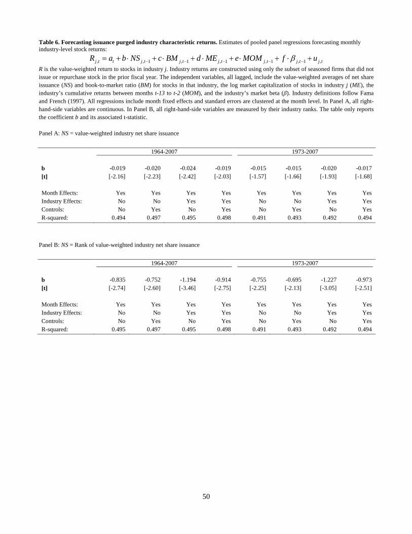
50

Table 6. Forecasting issuance purged industry characteristic returns. Estimates of pooled panel regressions forecasting monthly industry-level stock returns:

, , 1 , 1 , 1 , 1 , 1 ,j t t j t j t j t j t j t j tR a b NS c BM d ME e MOM f uβ− − − − −= + ⋅ + ⋅ + ⋅ + ⋅ + ⋅ +

R is the value-weighted return to stocks in industry j. Industry returns are constructed using only the subset of seasoned firms that did not issue or repurchase stock in the prior fiscal year. The independent variables, all lagged, include the value-weighted averages of net share issuance (NS) and book-to-market ratio (BM) for stocks in that industry, the log market capitalization of stocks in industry j (ME), the industry’s cumulative returns between months t-13 to t-2 (MOM), and the industry’s market beta (β). Industry definitions follow Fama and French (1997). All regressions include month fixed effects and standard errors are clustered at the month level. In Panel A, all right-hand-side variables are continuous. In Panel B, all right-hand-side variables are measured by their industry ranks. The table only reports the coefficient b and its associated t-statistic.

Panel A: NS = value-weighted industry net share issuance

1964-2007 1973-2007 b -0.019 -0.020 -0.024 -0.019 -0.015 -0.015 -0.020 -0.017 [t] [-2.16] [-2.23] [-2.42] [-2.03] [-1.57] [-1.66] [-1.93] [-1.68] Month Effects: Yes Yes Yes Yes Yes Yes Yes Yes Industry Effects: No No Yes Yes No No Yes Yes Controls: No Yes No Yes No Yes No Yes R-squared: 0.494 0.497 0.495 0.498 0.491 0.493 0.492 0.494

Panel B: NS = Rank of value-weighted industry net share issuance

1964-2007 1973-2007 b -0.835 -0.752 -1.194 -0.914 -0.755 -0.695 -1.227 -0.973 [t] [-2.74] [-2.60] [-3.46] [-2.75] [-2.25] [-2.13] [-3.05] [-2.51] Month Effects: Yes Yes Yes Yes Yes Yes Yes Yes Industry Effects: No No Yes Yes No No Yes Yes Controls: No Yes No Yes No Yes No Yes R-squared: 0.495 0.497 0.495 0.498 0.491 0.493 0.492 0.494

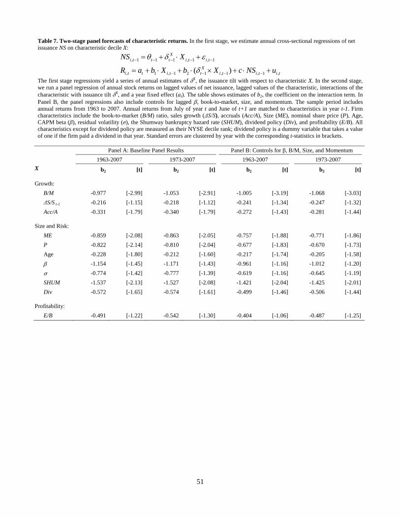
51

Table 7. Two-stage panel forecasts of characteristic returns. In the first stage, we estimate annual cross-sectional regressions of net issuance NS on characteristic decile X:

, 1 1 1 , 1 , 1

, 1 , 1 2 1 , 1 , 1 ,( )

Xi t t t i t i t

Xi t t i t t i t i t i t

NS X

R a b X b X c NS u

θ δ ε

δ− − − − −

− − − −

= + ⋅ +

= + ⋅ + ⋅ × + ⋅ +

The first stage regressions yield a series of annual estimates of δX, the issuance tilt with respect to characteristic X. In the second stage, we run a panel regression of annual stock returns on lagged values of net issuance, lagged values of the characteristic, interactions of the characteristic with issuance tilt δX, and a year fixed effect (at). The table shows estimates of b2, the coefficient on the interaction term. In Panel B, the panel regressions also include controls for lagged β, book-to-market, size, and momentum. The sample period includes annual returns from 1963 to 2007. Annual returns from July of year t and June of t+1 are matched to characteristics in year t-1. Firm characteristics include the book-to-market (B/M) ratio, sales growth (ΔS/S), accruals (Acc/A), Size (ME), nominal share price (P), Age, CAPM beta (β), residual volatility (σ), the Shumway bankruptcy hazard rate (SHUM), dividend policy (Div), and profitability (E/B). All characteristics except for dividend policy are measured as their NYSE decile rank; dividend policy is a dummy variable that takes a value of one if the firm paid a dividend in that year. Standard errors are clustered by year with the corresponding t-statistics in brackets.

Panel A: Baseline Panel Results Panel B: Controls for β, B/M, Size, and Momentum 1963-2007 1973-2007 1963-2007 1973-2007 X b2 [t] b2 [t] b2 [t] b2 [t]

Growth:

B/M -0.977 [-2.99] -1.053 [-2.91] -1.005 [-3.19] -1.068 [-3.03] ΔS/S t-1 -0.216 [-1.15] -0.218 [-1.12] -0.241 [-1.34] -0.247 [-1.32] Acc/A -0.331 [-1.79] -0.340 [-1.79] -0.272 [-1.43] -0.281 [-1.44]

Size and Risk: ME -0.859 [-2.08] -0.863 [-2.05] -0.757 [-1.88] -0.771 [-1.86] P -0.822 [-2.14] -0.810 [-2.04] -0.677 [-1.83] -0.670 [-1.73] Age -0.228 [-1.80] -0.212 [-1.60] -0.217 [-1.74] -0.205 [-1.58]

β -1.154 [-1.45] -1.171 [-1.43] -0.961 [-1.16] -1.012 [-1.20]

σ -0.774 [-1.42] -0.777 [-1.39] -0.619 [-1.16] -0.645 [-1.19] SHUM -1.537 [-2.13] -1.527 [-2.08] -1.421 [-2.04] -1.425 [-2.01] Div -0.572 [-1.65] -0.574 [-1.61] -0.499 [-1.46] -0.506 [-1.44]

Profitability: E/B -0.491 [-1.22] -0.542 [-1.30] -0.404 [-1.06] -0.487 [-1.25]

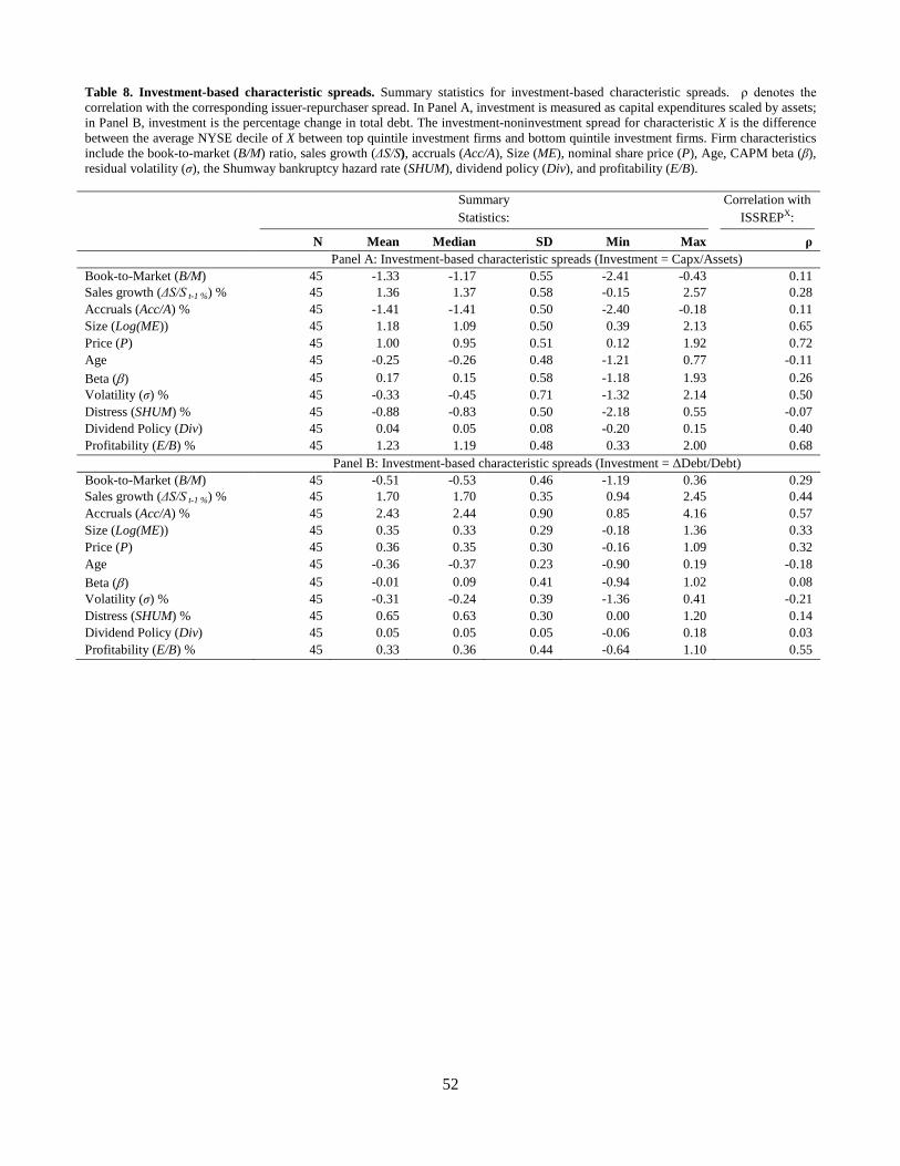
52

Table 8. Investment-based characteristic spreads. Summary statistics for investment-based characteristic spreads. ρ denotes the correlation with the corresponding issuer-repurchaser spread. In Panel A, investment is measured as capital expenditures scaled by assets; in Panel B, investment is the percentage change in total debt. The investment-noninvestment spread for characteristic X is the difference between the average NYSE decile of X between top quintile investment firms and bottom quintile investment firms. Firm characteristics include the book-to-market (B/M) ratio, sales growth (ΔS/S), accruals (Acc/A), Size (ME), nominal share price (P), Age, CAPM beta (β), residual volatility (σ), the Shumway bankruptcy hazard rate (SHUM), dividend policy (Div), and profitability (E/B).

Summary Statistics:

Correlation with ISSREPX:

N Mean Median SD Min Max ρ Panel A: Investment-based characteristic spreads (Investment = Capx/Assets) Book-to-Market (B/M) 45 -1.33 -1.17 0.55 -2.41 -0.43 0.11 Sales growth (ΔS/S t-1 %) % 45 1.36 1.37 0.58 -0.15 2.57 0.28 Accruals (Acc/A) % 45 -1.41 -1.41 0.50 -2.40 -0.18 0.11 Size (Log(ME)) 45 1.18 1.09 0.50 0.39 2.13 0.65 Price (P) 45 1.00 0.95 0.51 0.12 1.92 0.72 Age 45 -0.25 -0.26 0.48 -1.21 0.77 -0.11 Beta (β) 45 0.17 0.15 0.58 -1.18 1.93 0.26 Volatility (σ) % 45 -0.33 -0.45 0.71 -1.32 2.14 0.50 Distress (SHUM) % 45 -0.88 -0.83 0.50 -2.18 0.55 -0.07 Dividend Policy (Div) 45 0.04 0.05 0.08 -0.20 0.15 0.40 Profitability (E/B) % 45 1.23 1.19 0.48 0.33 2.00 0.68 Panel B: Investment-based characteristic spreads (Investment = ΔDebt/Debt) Book-to-Market (B/M) 45 -0.51 -0.53 0.46 -1.19 0.36 0.29 Sales growth (ΔS/S t-1 %) % 45 1.70 1.70 0.35 0.94 2.45 0.44 Accruals (Acc/A) % 45 2.43 2.44 0.90 0.85 4.16 0.57 Size (Log(ME)) 45 0.35 0.33 0.29 -0.18 1.36 0.33 Price (P) 45 0.36 0.35 0.30 -0.16 1.09 0.32 Age 45 -0.36 -0.37 0.23 -0.90 0.19 -0.18 Beta (β) 45 -0.01 0.09 0.41 -0.94 1.02 0.08 Volatility (σ) % 45 -0.31 -0.24 0.39 -1.36 0.41 -0.21 Distress (SHUM) % 45 0.65 0.63 0.30 0.00 1.20 0.14 Dividend Policy (Div) 45 0.05 0.05 0.05 -0.06 0.18 0.03 Profitability (E/B) % 45 0.33 0.36 0.44 -0.64 1.10 0.55

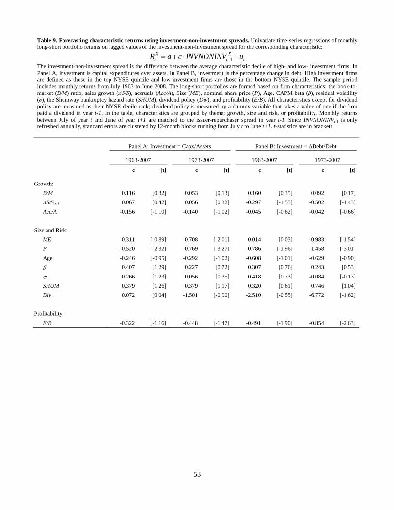
53

Table 9. Forecasting characteristic returns using investment-non-investment spreads. Univariate time-series regressions of monthly long-short portfolio returns on lagged values of the investment-non-investment spread for the corresponding characteristic:

1X X

t t tR a c INVNONINV u−= + ⋅ +

The investment-non-investment spread is the difference between the average characteristic decile of high- and low- investment firms. In Panel A, investment is capital expenditures over assets. In Panel B, investment is the percentage change in debt. High investment firms are defined as those in the top NYSE quintile and low investment firms are those in the bottom NYSE quintile. The sample period includes monthly returns from July 1963 to June 2008. The long-short portfolios are formed based on firm characteristics: the book-to-market (B/M) ratio, sales growth (ΔS/S), accruals (Acc/A), Size (ME), nominal share price (P), Age, CAPM beta (β), residual volatility (σ), the Shumway bankruptcy hazard rate (SHUM), dividend policy (Div), and profitability (E/B). All characteristics except for dividend policy are measured as their NYSE decile rank; dividend policy is measured by a dummy variable that takes a value of one if the firm paid a dividend in year t-1. In the table, characteristics are grouped by theme: growth, size and risk, or profitability. Monthly returns between July of year t and June of year t+1 are matched to the issuer-repurchaser spread in year t-1. Since INVNONINVt-1 is only refreshed annually, standard errors are clustered by 12-month blocks running from July t to June t+1. t-statistics are in brackets.

Panel A: Investment = Capx/Assets Panel B: Investment = ΔDebt/Debt

1963-2007 1973-2007 1963-2007 1973-2007 c [t] c [t] c [t] c [t]

Growth: B/M 0.116 [0.32] 0.053 [0.13] 0.160 [0.35] 0.092 [0.17] ΔS/S t-1 0.067 [0.42] 0.056 [0.32] -0.297 [-1.55] -0.502 [-1.43] Acc/A -0.156 [-1.10] -0.140 [-1.02] -0.045 [-0.62] -0.042 [-0.66]

Size and Risk: ME -0.311 [-0.89] -0.708 [-2.01] 0.014 [0.03] -0.983 [-1.54] P -0.520 [-2.32] -0.769 [-3.27] -0.786 [-1.96] -1.458 [-3.01] Age -0.246 [-0.95] -0.292 [-1.02] -0.608 [-1.01] -0.629 [-0.90]

β 0.407 [1.29] 0.227 [0.72] 0.307 [0.76] 0.243 [0.53]

σ 0.266 [1.23] 0.056 [0.35] 0.418 [0.73] -0.084 [-0.13] SHUM 0.379 [1.26] 0.379 [1.17] 0.320 [0.61] 0.746 [1.04] Div 0.072 [0.04] -1.501 [-0.90] -2.510 [-0.55] -6.772 [-1.62]

Profitability: E/B -0.322 [-1.16] -0.448 [-1.47] -0.491 [-1.90] -0.854 [-2.63]

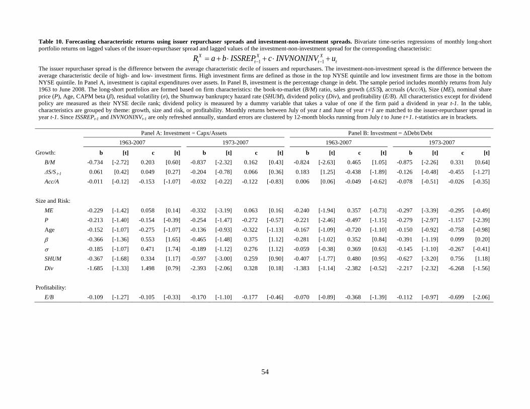
54

Table 10. Forecasting characteristic returns using issuer repurchaser spreads and investment-non-investment spreads. Bivariate time-series regressions of monthly long-short portfolio returns on lagged values of the issuer-repurchaser spread and lagged values of the investment-non-investment spread for the corresponding characteristic:

1 1X X X

t t t tR a b ISSREP c INVNONINV u− −= + ⋅ + ⋅ +

The issuer repurchaser spread is the difference between the average characteristic decile of issuers and repurchasers. The investment-non-investment spread is the difference between the average characteristic decile of high- and low- investment firms. High investment firms are defined as those in the top NYSE quintile and low investment firms are those in the bottom NYSE quintile. In Panel A, investment is capital expenditures over assets. In Panel B, investment is the percentage change in debt. The sample period includes monthly returns from July 1963 to June 2008. The long-short portfolios are formed based on firm characteristics: the book-to-market (B/M) ratio, sales growth (ΔS/S), accruals (Acc/A), Size (ME), nominal share price (P), Age, CAPM beta (β), residual volatility (σ), the Shumway bankruptcy hazard rate (SHUM), dividend policy (Div), and profitability (E/B). All characteristics except for dividend policy are measured as their NYSE decile rank; dividend policy is measured by a dummy variable that takes a value of one if the firm paid a dividend in year t-1. In the table, characteristics are grouped by theme: growth, size and risk, or profitability. Monthly returns between July of year t and June of year t+1 are matched to the issuer-repurchaser spread in year t-1. Since ISSREPt-1 and INVNONINVt-1 are only refreshed annually, standard errors are clustered by 12-month blocks running from July t to June t+1. t-statistics are in brackets.

Panel A: Investment = Capx/Assets Panel B: Investment = ΔDebt/Debt

1963-2007 1973-2007 1963-2007 1973-2007

Growth: b [t] c [t] b [t] c [t] b [t] c [t] b [t] c [t] B/M -0.734 [-2.72] 0.203 [0.60] -0.837 [-2.32] 0.162 [0.43] -0.824 [-2.63] 0.465 [1.05] -0.875 [-2.26] 0.331 [0.64] ΔS/S t-1 0.061 [0.42] 0.049 [0.27] -0.204 [-0.78] 0.066 [0.36] 0.183 [1.25] -0.438 [-1.89] -0.126 [-0.48] -0.455 [-1.27] Acc/A -0.011 [-0.12] -0.153 [-1.07] -0.032 [-0.22] -0.122 [-0.83] 0.006 [0.06] -0.049 [-0.62] -0.078 [-0.51] -0.026 [-0.35]

Size and Risk: ME -0.229 [-1.42] 0.058 [0.14] -0.332 [-3.19] 0.063 [0.16] -0.240 [-1.94] 0.357 [-0.73] -0.297 [-3.39] -0.295 [-0.49] P -0.213 [-1.40] -0.154 [-0.39] -0.254 [-1.47] -0.272 [-0.57] -0.221 [-2.46] -0.497 [-1.15] -0.279 [-2.97] -1.157 [-2.39] Age -0.152 [-1.07] -0.275 [-1.07] -0.136 [-0.93] -0.322 [-1.13] -0.167 [-1.09] -0.720 [-1.10] -0.150 [-0.92] -0.758 [-0.98]

β -0.366 [-1.36] 0.553 [1.65] -0.465 [-1.48] 0.375 [1.12] -0.281 [-1.02] 0.352 [0.84] -0.391 [-1.19] 0.099 [0.20]

σ -0.185 [-1.07] 0.471 [1.74] -0.189 [-1.12] 0.276 [1.12] -0.059 [-0.38] 0.369 [0.63] -0.145 [-1.10] -0.267 [-0.41] SHUM -0.367 [-1.68] 0.334 [1.17] -0.597 [-3.00] 0.259 [0.90] -0.407 [-1.77] 0.480 [0.95] -0.627 [-3.20] 0.756 [1.18] Div -1.685 [-1.33] 1.498 [0.79] -2.393 [-2.06] 0.328 [0.18] -1.383 [-1.14] -2.382 [-0.52] -2.217 [-2.32] -6.268 [-1.56]

Profitability: E/B -0.109 [-1.27] -0.105 [-0.33] -0.170 [-1.10] -0.177 [-0.46] -0.070 [-0.89] -0.368 [-1.39] -0.112 [-0.97] -0.699 [-2.06]

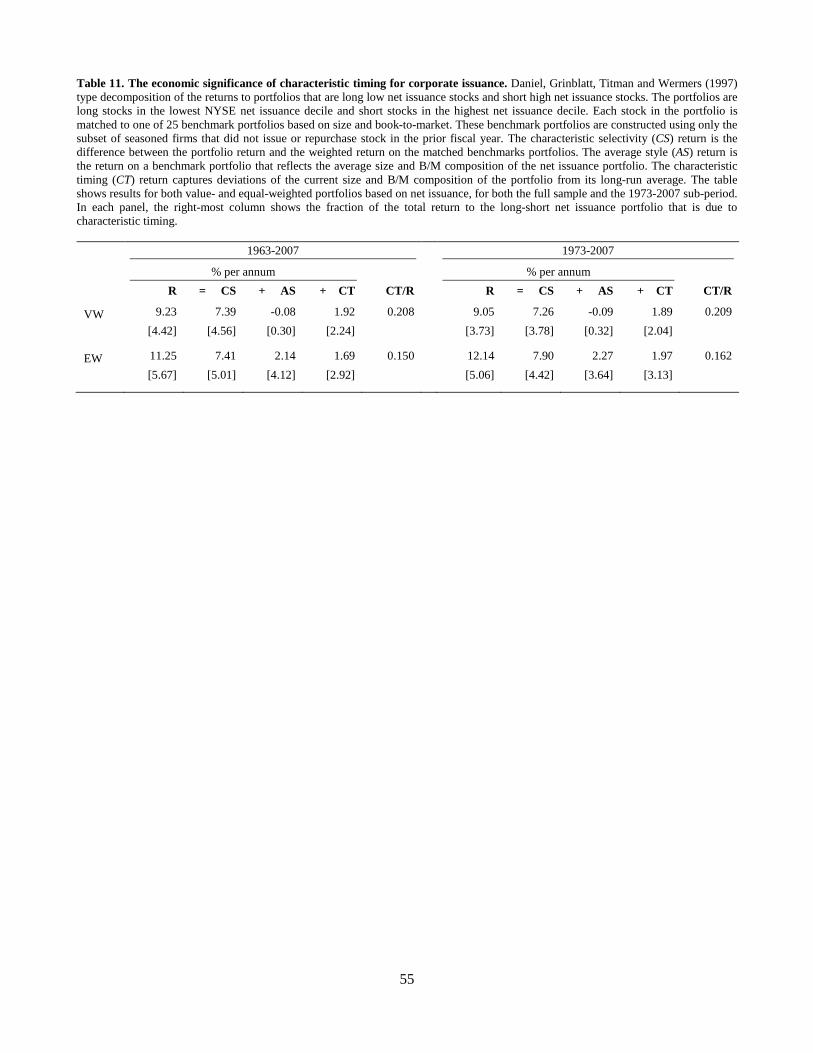
55

Table 11. The economic significance of characteristic timing for corporate issuance. Daniel, Grinblatt, Titman and Wermers (1997) type decomposition of the returns to portfolios that are long low net issuance stocks and short high net issuance stocks. The portfolios are long stocks in the lowest NYSE net issuance decile and short stocks in the highest net issuance decile. Each stock in the portfolio is matched to one of 25 benchmark portfolios based on size and book-to-market. These benchmark portfolios are constructed using only the subset of seasoned firms that did not issue or repurchase stock in the prior fiscal year. The characteristic selectivity (CS) return is the difference between the portfolio return and the weighted return on the matched benchmarks portfolios. The average style (AS) return is the return on a benchmark portfolio that reflects the average size and B/M composition of the net issuance portfolio. The characteristic timing (CT) return captures deviations of the current size and B/M composition of the portfolio from its long-run average. The table shows results for both value- and equal-weighted portfolios based on net issuance, for both the full sample and the 1973-2007 sub-period. In each panel, the right-most column shows the fraction of the total return to the long-short net issuance portfolio that is due to characteristic timing.

1963-2007 1973-2007 % per annum % per annum R = CS + AS + CT CT/R R = CS + AS + CT CT/R

VW 9.23 7.39 -0.08 1.92 0.208 9.05 7.26 -0.09 1.89 0.209

[4.42] [4.56] [0.30] [2.24] [3.73] [3.78] [0.32] [2.04]

EW 11.25 7.41 2.14 1.69 0.150 12.14 7.90 2.27 1.97 0.162

[5.67] [5.01] [4.12] [2.92] [5.06] [4.42] [3.64] [3.13]