Embed Size (px)
Citation preview
273
Chapter 7Random Variables and
Selected Probability Models
In this chapter we further develop our understanding of probability by presenting theconcept of discrete and continuous random variables. As we shall see presently, randomvariables are those whose numerical values are in some sense governed by a probabilisticmechanism. In some cases this mechanism takes a definite mathematical form which isreferred to as a probability model. We shall describe two such models that apply todiscrete random variables - the Binomial and Poisson models. We shall also consider theGaussian probability model which depicts the probabilistic behaviour of certaincontinuous random variables. Some time will be devoted to the expectations operator.This is a special mathematical tool used to calculate the mean and variance of randomvariables. We shall also learn how the expectations operator may be used to facilitatebusiness decision making within a real estate setting. Finally, some discussion will bedevoted to the use of EXCEL and the HP - 10B in areas related to this chapter.
7.1 Random Variables
A random variable x may be thought of as the numerical value of a function which isdefined on a sample space S generated by an experiment.
More formally, the ith value of a random variable is defined as :
xi = f(Ei) where : Ei ∈ S
This rather abstract idea may be illustrated with a very simple example. Consider anexperiment in which two tenants are randomly selected (without replacement) from thepopulation of ten tenants in a medium sized office building.
Let T1 (T2) = 1 if the first (second) of these tenants drawn from the population isagreeable to a lease variation proposed by the owner of the building. Let T1 (T2) = 0 if thefirst (second) tenant is not agreeable.
Now the sample space generated by this experiment comprises the following four pairs :
S = {(T1, T2) : (0,1) (1,0) (1,1) (0,0)}
and the random variable x is the number of agreeable tenants generated by theexperiment.
The numerical function defined on the sample space S - denoted : f(T1, T2) = T1 + T2 -maps the sample points (i.e. the pairs (T1, T2) into x-values as indicated in Figure 7.1.
274 Chapter 7
Figure 7.1 : Depiction of a Random Variable as a Numerical Functionthat Maps Sample Points {Ei} in the Sample Space S into Numerical Values {xi}
(0,1)
(1,0)
(1,1)
(0,0)
x = 1
x = 2
x = 0
f(T1, T 2) = T1 + T2 = x
S =
xi{ }Ei{ }
Note that each x-value corresponds to some elementary event or a set of elementaryevents. For example x = 1 is associated with the set of events : {(1, 0) (0, 1)} Moreover, x= 0 is associated with event (0,0). Now if these events occur with a specific probability, wemay assign probabilities to the various values of x. For example, suppose that 5 of the 10tenants would be agreeable to the lease variation. Then :
Pr(x=0) = Pr(T1 = 0 ∩ T2 = 0) = Pr(T1 = 0) Pr(T2 = 0 | T1 = 0) = 510 x
49 =
2090
Pr(x=1) = Pr(T1 = 1 ∩ T2 = 0) + Pr(T1 = 0 ∩ T2 = 1) = Pr(T1 = 1)Pr(T2= 0 | T1 = 1) + Pr(T1 = 0)Pr(T2 = 1 | T1 = 0)
= 510 x
59 + 5
10 x 59 =
2590 +
2590 =
5090
Pr(x=0) = Pr(T1 = 1 ∩ T2 = 1) = Pr(T1 = 1) Pr(T2 = 1 | T1 = 1) = 510 x
49 =
2090
The Probability Distribution of a Random Variable x
The probability distribution of a random variable x is the set of ordered pairs :
{ (xi, Pr(xi) }
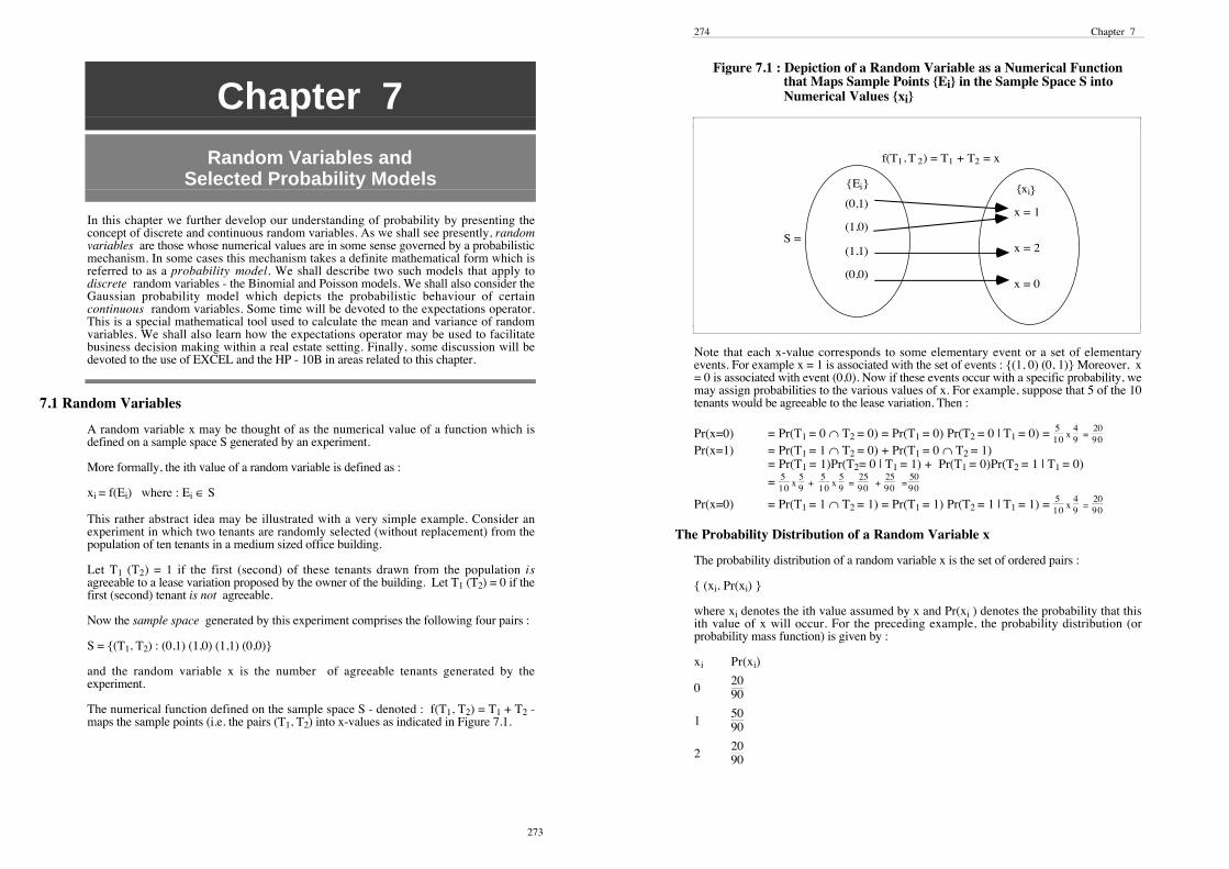
where xi denotes the ith value assumed by x and Pr(xi ) denotes the probability that thisith value of x will occur. For the preceding example, the probability distribution (orprobability mass function) is given by :
xi Pr(xi)
02090
15090
22090
Random Variables and Selected Probability Models 275
The probability mass function may also be presented graphically. For the probabilitydistribution we have just considered, its graphical analogue is reproduced in Figure 7.2 :
Figure 7.2 Graphical Presentation of a Probability Mass Function
0 1 2
50/90
40/90
30/90
20/90
10/90
0
Pr ( x )i
ix
•
•
•
The Expected Value of a Random Variable x
The expected value of a random variable x - denoted E(x) - is its arithmetic mean µobtained by taking a weighted average of the xi's using the associated Pr(xi)'s as weights.Symbolically we write :
E(x) = ΣPr(xi)⋅xi
We may illustrate the concept of expected value by considering management of arestaurant franchise operation that has employed the empirical approach to generate theprobability distribution of the internal rate of return xi of a restaurant1 in the franchisechain. This distribution is reproduced in Table 7.1.
From this table the expected internal rate of return of a restaurant in the chain is givendirectly below :
E(x) = ΣPr(xi)⋅xi = (-.05)(.05) + (.05)(.15) + (.15)(.30) + (.20)(.50)
= -.0025 + .0075 + .045 +.10 = .15
The variance of a random variable x - denoted V(x) - is the mean squared deviation of thevariable x from its expected value (or mean). More formally, we may write :
V(x) = E([x -E(x)]2)
1 The internal rate of return is the rate of profitability of an investment. For simplicity suppose onewere to plough half a million dollars into a restaurant operation that one expects will return a profit of$50,000 for ever (sic). Then the rate of profitability or internal rate of return would be 10% or .10expressed decimally.
276 Chapter 7
Table 7.1 Probability Distribution for the Internal Rate of Return x
xi Pr(xi)
- .05 .05
+.05 .15
+.15 .30
+.20 .50
The expression on the right hand side of this expression may be expanded as follows :
E{[x -E(x)]2} = E{x2 -2E(x)⋅x + [E(x)]2}
= E(x2) -2[E(x)]2 + [E(x)]2 = E(x2) - [E(x)]2
where : E(x2) = ΣPr(xi)⋅x2i and [E(x)]2 = [ΣPr(xi)⋅xi]2
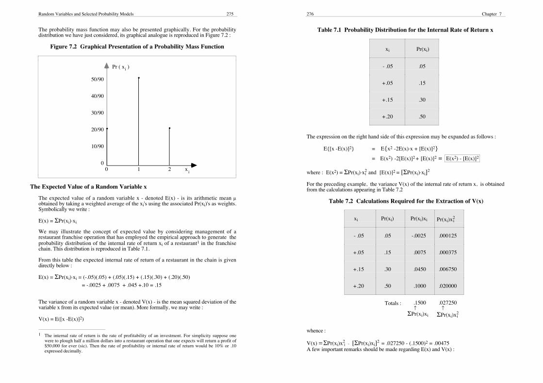
For the preceding example, the variance V(x) of the internal rate of return x, is obtainedfrom the calculations appearing in Table 7.2
Table 7.2 Calculations Required for the Extraction of V(x)
xi Pr(xi) Pr(xi)xi Pr(xi)x2i
- .05 .05 -.0025 .000125
+.05 .15 .0075 .000375
+.15 .30 .0450 .006750
+.20 .50 .1000 .020000
Totals : .1500 ↑ΣPr(xi)xi
.027250 ↑ΣPr(xi)x
2i
whence :
V(x) = ΣPr(xi)x2i - [ΣPr(xi)xi]2 = .027250 - (.1500)2 = .00475
A few important remarks should be made regarding E(x) and V(x) :
Random Variables and Selected Probability Models 277
Remark 1
From Chapter 4 it should be recalled that the variance is the square of the standarddeviation σ. In terms of the expectations operator : E(x) we may define σ as follows :
σ = √⎯⎯⎯⎯V(x) = √⎯⎯⎯⎯⎯⎯⎯⎯⎯E{[x - E(x)]2} = √⎯⎯⎯⎯⎯⎯⎯⎯⎯E(x2) - [E(x)]2.
Hence, for our restaurant franchise example, the standard deviation of the internal rate ofreturn is given by :
√⎯⎯⎯⎯⎯⎯.00475 = .06892 ≈ .07.
That is, the internal rate of return of restaurants in the chain is expected to vary 'on theaverage' within the range : .08 and .22 (i.e. .15 ± .07).
Remark 2
The standard random variable z is defined as one whose expected value is zero (i.e. E(z)= 0) and its variance is unity (i.e. V(z) = 1). Any random variable x may be converted intothe standard random variable z by applying the following transformation :
z = x - E(x)
√⎯⎯⎯⎯V( )x .
This transformation process is referred to as the standardisation of the random variablex. Later in this chapter we shall have much more to say about it.
Remark 3
If x and y are random variables, then for any given constants a and b the following rules -stated without proof - hold :
Rule 1 : E(a ± bx) = a ± bE(x)
To illustrate this rule, suppose demand for a recreational site (measured in number ofannual visits) is given by :
a + bx = 50000+ 20000x
where : a = 50000b = 20000x = 1 (0) if the weather in summer is good(poor)
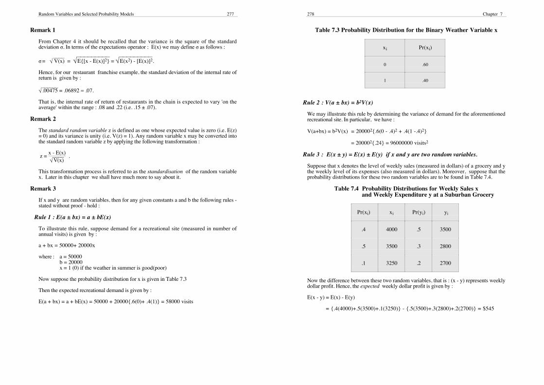
Now suppose the probability distribution for x is given in Table 7.3
Then the expected recreational demand is given by :
E(a + bx) = a + bE(x) = 50000 + 20000{.6(0)+ .4(1)} = 58000 visits
278 Chapter 7
Table 7.3 Probability Distribution for the Binary Weather Variable x
xi Pr(xi)
0 .60
1 .40
Rule 2 : V(a ± bx) = b2V(x)
We may illustrate this rule by determining the variance of demand for the aforementionedrecreational site. In particular, we have :
V(a+bx) = b2V(x) = 200002{.6(0 - .4)2 + .4(1 -.4)2}
= 200002{.24} = 96000000 visits2
Rule 3 : E(x ± y) = E(x) ± E(y) if x and y are two random variables.
Suppose that x denotes the level of weekly sales (measured in dollars) of a grocery and ythe weekly level of its expenses (also measured in dollars). Moreover, suppose that theprobability distributions for these two random variables are to be found in Table 7.4.
Table 7.4 Probability Distributions for Weekly Sales xand Weekly Expenditure y at a Suburban Grocery
Pr(xi) xi Pr(yi) yi
.4 4000 .5 3500
.5 3500 .3 2800
.1 3250 .2 2700
Now the difference between these two random variables, that is : (x - y) represents weeklydollar profit. Hence, the expected weekly dollar profit is given by :
E(x - y) = E(x) - E(y)
= {.4(4000)+.5(3500)+.1(3250)} - {.5(3500)+.3(2800)+.2(2700)} = $545
Random Variables and Selected Probability Models 279
Rule 4 : V(x ± y) = V(x) + V(y) if x and y are independent random variables 2
We may illustrate this rule by returning to our grocery example. Specifically, suppose wewish to determine the variance of weekly grocery profit. Then, if sales and expenses maybe regarded as independent random variables we may apply Rule 4 as follows :
V(x - y) = V(x) + V(y) = {E(x2) - [E(x)]2} + {E(y2) - [E(y)]2} = 75625 + 138100 = 213725 dollars2
where :
E(x) = .4(4000)+.5(3500)+.1(3250) = 3675[E(x)]2 = 36752 = 13505625E(x2) = .4(4000)2 +.5(3500)2 +.1(3250)2 = 13581250E(y) = .5(3500) +.3(2800)+.2(2700) = 3130[E(y)]2 = 31302 = 9796900E(y2) = .5(3500)2 +.3(2800)2 +.2(2700)2 = 9935000
Using E(x) and V(x) to Facilitate Business Decision Making
When the random variable under study represents income or profit (measured in dollars),the operators E(x) and V(x) may be used to facilitate business decision making when itcomes to selecting the optimal business undertaking from a choice set of competingalternatives.
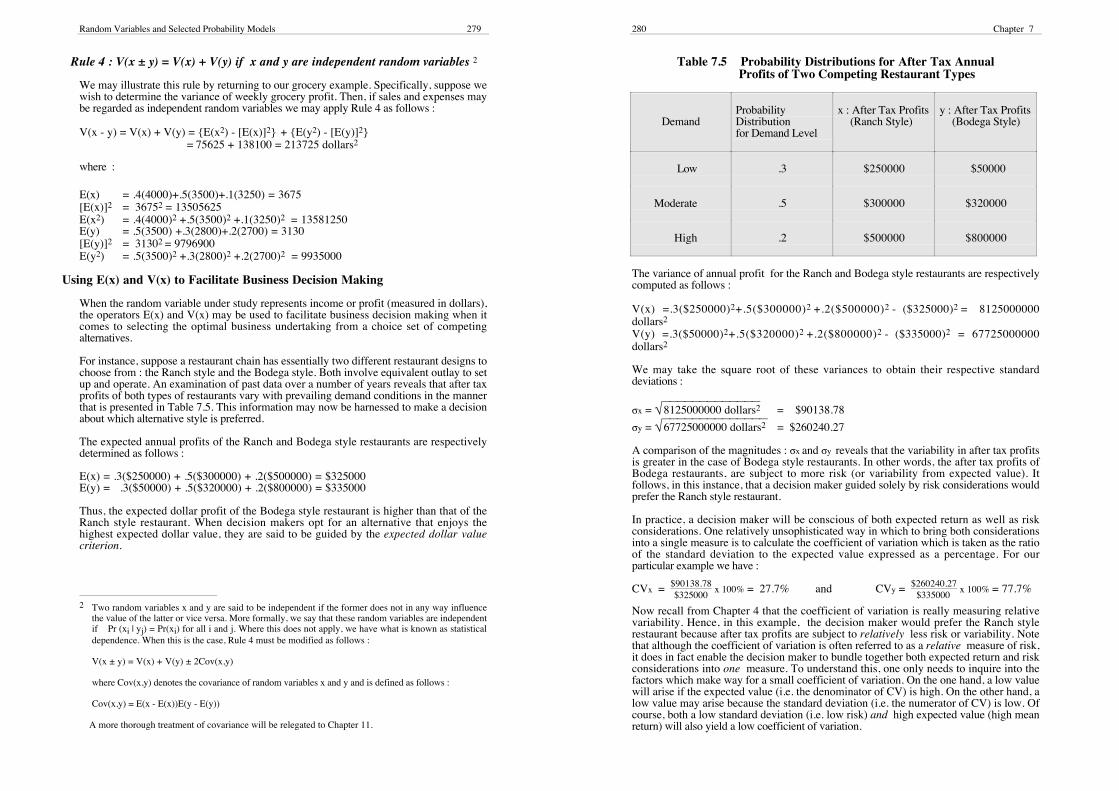
For instance, suppose a restaurant chain has essentially two different restaurant designs tochoose from : the Ranch style and the Bodega style. Both involve equivalent outlay to setup and operate. An examination of past data over a number of years reveals that after taxprofits of both types of restaurants vary with prevailing demand conditions in the mannerthat is presented in Table 7.5. This information may now be harnessed to make a decisionabout which alternative style is preferred.
The expected annual profits of the Ranch and Bodega style restaurants are respectivelydetermined as follows :
E(x) = .3($250000) + .5($300000) + .2($500000) = $325000E(y) = .3($50000) + .5($320000) + .2($800000) = $335000
Thus, the expected dollar profit of the Bodega style restaurant is higher than that of theRanch style restaurant. When decision makers opt for an alternative that enjoys thehighest expected dollar value, they are said to be guided by the expected dollar valuecriterion.
2 Two random variables x and y are said to be independent if the former does not in any way influencethe value of the latter or vice versa. More formally, we say that these random variables are independentif Pr (xi | yj) = Pr(xi) for all i and j. Where this does not apply, we have what is known as statisticaldependence. When this is the case, Rule 4 must be modified as follows :
V(x ± y) = V(x) + V(y) ± 2Cov(x,y)
where Cov(x,y) denotes the covariance of random variables x and y and is defined as follows :
Cov(x,y) = E(x - E(x))E(y - E(y))
A more thorough treatment of covariance will be relegated to Chapter 11.
280 Chapter 7
Table 7.5 Probability Distributions for After Tax Annual Profits of Two Competing Restaurant Types
DemandProbabilityDistributionfor Demand Level
x : After Tax Profits(Ranch Style)
y : After Tax Profits(Bodega Style)
Low .3 $250000 $50000
Moderate .5 $300000 $320000
High .2 $500000 $800000
The variance of annual profit for the Ranch and Bodega style restaurants are respectivelycomputed as follows :
V(x) =.3($250000)2+.5($300000)2 +.2($500000)2 - ($325000)2 = 8125000000dollars2
V(y) =.3($50000)2+.5($320000)2 +.2($800000)2 - ($335000)2 = 67725000000dollars2
We may take the square root of these variances to obtain their respective standarddeviations :
σx = √⎯⎯⎯⎯⎯⎯⎯⎯⎯⎯⎯⎯⎯8125000000 dollars2 = $90138.78
σy = √⎯⎯⎯⎯⎯⎯⎯⎯⎯⎯⎯⎯⎯⎯67725000000 dollars2 = $260240.27
A comparison of the magnitudes : σx and σy reveals that the variability in after tax profitsis greater in the case of Bodega style restaurants. In other words, the after tax profits ofBodega restaurants, are subject to more risk (or variability from expected value). Itfollows, in this instance, that a decision maker guided solely by risk considerations wouldprefer the Ranch style restaurant.
In practice, a decision maker will be conscious of both expected return as well as riskconsiderations. One relatively unsophisticated way in which to bring both considerationsinto a single measure is to calculate the coefficient of variation which is taken as the ratioof the standard deviation to the expected value expressed as a percentage. For ourparticular example we have :
CVx = $90138.78$325000
x 100% = 27.7% and CVy = $260240.27$335000
x 100% = 77.7%
Now recall from Chapter 4 that the coefficient of variation is really measuring relativevariability. Hence, in this example, the decision maker would prefer the Ranch stylerestaurant because after tax profits are subject to relatively less risk or variability. Notethat although the coefficient of variation is often referred to as a relative measure of risk,it does in fact enable the decision maker to bundle together both expected return and riskconsiderations into one measure. To understand this, one only needs to inquire into thefactors which make way for a small coefficient of variation. On the one hand, a low valuewill arise if the expected value (i.e. the denominator of CV) is high. On the other hand, alow value may arise because the standard deviation (i.e. the numerator of CV) is low. Ofcourse, both a low standard deviation (i.e. low risk) and high expected value (high meanreturn) will also yield a low coefficient of variation.
Random Variables and Selected Probability Models 281
Continuous Random Variables
So far we have dealt with discrete random variables. These are variables that take a finitenumber of values. An experiment may also generate continuous random variables. That is,random variables that take on an uncountable number of values.
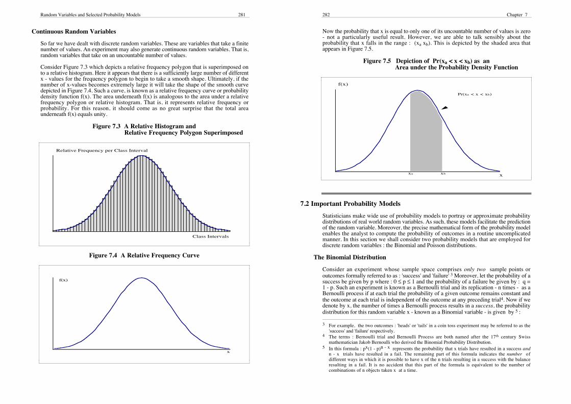
Consider Figure 7.3 which depicts a relative frequency polygon that is superimposed onto a relative histogram. Here it appears that there is a sufficiently large number of differentx - values for the frequency polygon to begin to take a smooth shape. Ultimately, if thenumber of x-values becomes extremely large it will take the shape of the smooth curvedepicted in Figure 7.4. Such a curve, is known as a relative frequency curve or probabilitydensity function f(x). The area underneath f(x) is analogous to the area under a relativefrequency polygon or relative histogram. That is, it represents relative frequency orprobability. For this reason, it should come as no great surprise that the total areaunderneath f(x) equals unity.
Figure 7.3 A Relative Histogram andRelative Frequency Polygon Superimposed
Relative Frequency per Class Interval
Class Intervals
Figure 7.4 A Relative Frequency Curve
f(x)
x
282 Chapter 7
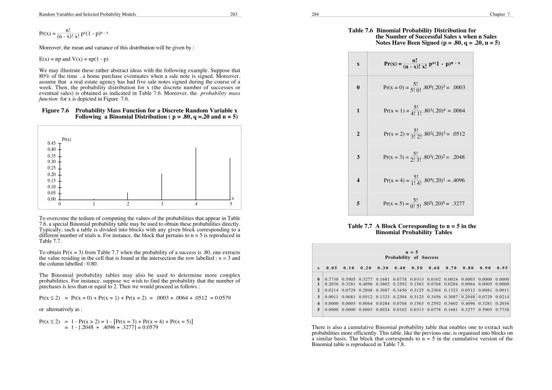
Now the probability that x is equal to only one of its uncountable number of values is zero- not a particularly useful result. However, we are able to talk sensibly about theprobability that x falls in the range : (xa xb). This is depicted by the shaded area thatappears in Figure 7.5.
Figure 7.5 Depiction of Pr(xa < x < xb) as anArea under the Probability Density Function
x
f(x)
Pr(xa < x < xb)
xa xb
7.2 Important Probability Models
Statisticians make wide use of probability models to portray or approximate probabilitydistributions of real world random variables. As such, these models facilitate the predictionof the random variable. Moreover, the precise mathematical form of the probability modelenables the analyst to compute the probability of outcomes in a routine uncomplicatedmanner. In this section we shall consider two probability models that are employed fordiscrete random variables : the Binomial and Poisson distributions.
The Binomial Distribution
Consider an experiment whose sample space comprises only two sample points oroutcomes formally referred to as : 'success' and 'failure' 3 Moreover, let the probability of asuccess be given by p where : 0 ≤ p ≤ 1 and the probability of a failure be given by : q =1 - p. Such an experiment is known as a Bernoulli trial and its replication - n times - as aBernoulli process if at each trial the probability of a given outcome remains constant andthe outcome at each trial is independent of the outcome at any preceding trial4. Now if wedenote by x, the number of times a Bernoulli process results in a success, the probabilitydistribution for this random variable x - known as a Binomial variable - is given by 5 :
3 For example, the two outcomes : 'heads' or 'tails' in a coin toss experiment may be referred to as the'success' and 'failure' respectively.
4 The terms : Bernoulli trial and Bernoulli Process are both named after the 17th century Swissmathematician Jakob Bernoulli who derived the Binomial Probability Distribution.
5 In this formula : px(1 - p)n - x represents the probability that x trials have resulted in a success andn - x trials have resulted in a fail. The remaining part of this formula indicates the number ofdifferent ways in which it is possible to have x of the n trials resulting in a success with the balanceresulting in a fail. It is no accident that this part of the formula is equivalent to the number ofcombinations of n objects taken x at a time.
Random Variables and Selected Probability Models 283
Pr(x) = n!
(n - x)! x! px(1 - p)n - x
Moreover, the mean and variance of this distribution will be given by :
E(x) = np and V(x) = np(1 - p)
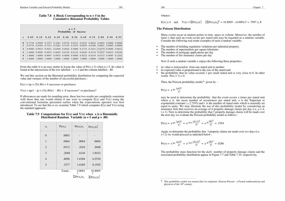
We may illustrate these rather abstract ideas with the following example. Suppose that80% of the time , a home purchase eventuates when a sale note is signed. Moreover,assume that a real estate agency has had five sale notes signed during the course of aweek. Then, the probability distribution for x (the discrete number of successes oreventual sales) is obtained as indicated in Table 7.6. Moreover, the probability massfunction for x is depicted in Figure 7.6.
Figure 7.6 Probability Mass Function for a Discrete Random Variable xFollowing a Binomial Distribution ( p = .80, q =.20 and n = 5)
0.000.050.100.150.200.250.300.350.400.45
0 1 2 3 4 5
Pr(x)
x
To overcome the tedium of computing the values of the probabilities that appear in Table7.6, a special Binomial probability table may be used to obtain these probabilities directly.Typically, such a table is divided into blocks with any given block corresponding to adifferent number of trials n. For instance, the block that pertains to n = 5 is reproduced inTable 7.7.
To obtain Pr(x = 3) from Table 7.7 when the probability of a success is .80, one extractsthe value residing in the cell that is found at the intersection the row labelled : x = 3 andthe column labelled : 0.80.
The Binomial probability tables may also be used to determine more complexprobabilities. For instance, suppose we wish to find the probability that the number ofpurchases is less than or equal to 2. Then we would proceed as follows :
Pr(x ≤ 2) = Pr(x = 0) + Pr(x = 1) + Pr(x = 2) = .0003 + .0064 + .0512 = 0.0579
or alternatively as :
Pr(x ≤ 2) = 1 - Pr(x > 2) = 1 - [Pr(x = 3) + Pr(x = 4) + Pr(x = 5)]= 1 - [.2048 + .4096 + .3277] = 0.0579
284 Chapter 7
Table 7.6 Binomial Probability Distribution forthe Number of Successful Sales x when n Sales
Notes Have Been Signed (p = .80, q = .20, n = 5)
x Pr(x) = n!
(n - x)! x! px(1 - p)n - x
0 Pr(x = 0) = 5!
5! 0! .800(.20)5 = .0003
1 Pr(x = 1) = 5!
4! 1! .801(.20)4 = .0064
2 Pr(x = 2) = 5!
3! 2! .802(.20)3 = .0512
3 Pr(x = 3) = 5!
2! 3! .803(.20)2 = .2048
4 Pr(x = 4) = 5!
1! 4! .804(.20)1 = .4096
5 Pr(x = 5) = 5!
0! 5! .805(.20)0 = .3277
Table 7.7 A Block Corresponding to n = 5 in theBinomial Probability Tables
n = 5Probability of Success
x 0 . 0 5 0 . 1 0 0 . 2 0 0 . 3 0 0 . 4 0 0 . 5 0 0 . 6 0 0 . 7 0 0 . 8 0 0 . 9 0 0 . 9 5
0 0.7738 0.5905 0.3277 0.1681 0.0778 0.0313 0.0102 0.0024 0.0003 0.0000 0.00001 0.2036 0.3281 0.4096 0.3602 0.2592 0.1563 0.0768 0.0284 0.0064 0.0005 0.0000
2 0.0214 0.0729 0.2048 0.3087 0.3456 0.3125 0.2304 0.1323 0.0512 0.0081 0.0011
3 0.0011 0.0081 0.0512 0.1323 0.2304 0.3125 0.3456 0.3087 0.2048 0.0729 0.0214
4 0.0000 0.0005 0.0064 0.0284 0.0768 0.1563 0.2592 0.3602 0.4096 0.3281 0.2036
5 0.0000 0.0000 0.0003 0.0024 0.0102 0.0313 0.0778 0.1681 0.3277 0.5905 0.7738
There is also a cumulative Binomial probability table that enables one to extract suchprobabilities more efficiently. This table, like the previous one, is organised into blocks ona similar basis. The block that corresponds to n = 5 in the cumulative version of theBinomial table is reproduced in Table 7.8.
Random Variables and Selected Probability Models 285
Table 7.8 A Block Corresponding to n = 5 in theCumulative Binomial Probability Tables
n = 5Probability of Success
x 0 . 0 5 0 . 1 0 0 . 2 0 0 . 3 0 0 . 4 0 0 . 5 0 0 . 6 0 0 . 7 0 0 . 8 0 0 . 9 0 0 . 9 5
0 0.7738 0.5905 0.3277 0.1681 0.0778 0.0313 0.0102 0.0024 0.0003 0.0000 0.00001 0.9774 0.9185 0.7373 0.5282 0.3370 0.1875 0.0870 0.0308 0.0067 0.0005 0.0000
2 0.9988 0.9914 0.9421 0.8369 0.6826 0.5000 0.3174 0.1631 0.0579 0.0086 0.0012
3 1.0000 0.9995 0.9933 0.9692 0.9130 0.8125 0.6630 0.4718 0.2627 0.0815 0.0226
4 1.0000 1.0000 0.9997 0.9976 0.9898 0.9688 0.9222 0.8319 0.6723 0.4095 0.2262
5 1.0000 1.0000 1.0000 1.0000 1.0000 1.0000 1.0000 1.0000 1.0000 1.0000 1.0000
From this table it is an easy matter to locate the value of Pr(x ≤ 2) when n = 5. Its value isfound at the intersection of the row labelled : x = 2 and the column labelled : .80.
We end this section on the Binomial probability distribution by computing the expectedvalue and variance of the number of successful purchases :
E(x) = np = (5)(.80) = 4 successes or purchases
V(x) = np(1 - p) = (5)(.80)(1 - .80) = .8 successes2 or purchases2
If allowances are made for rounding error, these last two results are completely consistentwith those that one would obtain if one were to compute E(x) and V(x) using theconventional formulae presented earlier when the expectations operator was firstintroduced. To see that this is so, examine Table 7.9 which computes E(x) and V(x) usingthe standard approach.
Table 7.9 Computations for E(x) and V(x) when x is a Binomially Distributed Random Variable (n = 5 and p = .80)
xi Pr(xi) Pr(xi)xi Pr(xi)x2i
0 .0003 - -
1 .0064 .0064 .0064
2 .0512 .1024 .2048
3 .2048 .6144 1.8432
4 .4096 1.6384 6.5536
5 .3277 1.6385 8.1925
Totals : 4.0001 ↑ΣPr(xi)xi
16.8005 ↑ΣPr(xi)x
2i
286 Chapter 7
whence :
E(x) ≅ 4 and V(x) = ΣPr(xi)x2i - [ΣPr(xi)xi]2 = 16.8005 - (4.0001)2 = .7997 ≅ .8
The Poisson Distribution
Many events occur at random points in time, space or volume. Moreover, the number oftimes x that such an event occurs per stated unit may be regarded as a random variable.Consider the following real estate examples of such a random variable :
• The number of building regulation violations per industrial property.• The number of supermarkets per square kilometre• The number of mortgage applications per day• The number of fire insurance claims per day
Now if such a random variable x enjoys the following three properties :
• its value is independent from one stated unit to another• its expected value is proportional to the size of the stated unit• the probability that its value exceeds 1 per small stated unit is very close to 0. In other
words Pr(x > 1) ≅ 0.
Then, the Poisson probability model 6 given by :
Pr(x) = e-µt (µt)x
x!
may be used to determine the probability that the event occurs x times per stated unitwhere µ is the mean number of occurrences per stated unit, e is the Napierian orexponential constant ( ≅ 2.7183) and t is the number of stated units which is normally setequal to unity. We may illustrate the use of this probability model by considering aninsurance firm that receives an average of 4 property damage claims per day (i.e. µ = 4,t = 1). Now to determine the probability that 3 property damage claims will be made overthe next day we evaluate the Poisson probability model as follows :
Pr(x) = e-µt (µt)x
x! = e-4x1 (4x1)3
3! = e-4 (4)3
3! = .1954
Again, to determine the probability that 3 property claims are made over two days (i.e.t = 2) we would proceed as indicated below :
Pr(x) = e-µt (µt)x
x! = e-4x2 (4x2)3
3! = e-8 (8)3
3! = .0286
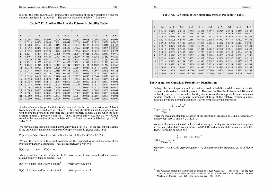
The probability mass function for the daily number of property damage claims and theassociated probability distribution appear in Figure 7.7 and Table 7.10 respectively.
6 This probability model was named after its originator, Simeon Poisson - a French mathematician andphysicist of the 18th century.
Random Variables and Selected Probability Models 287
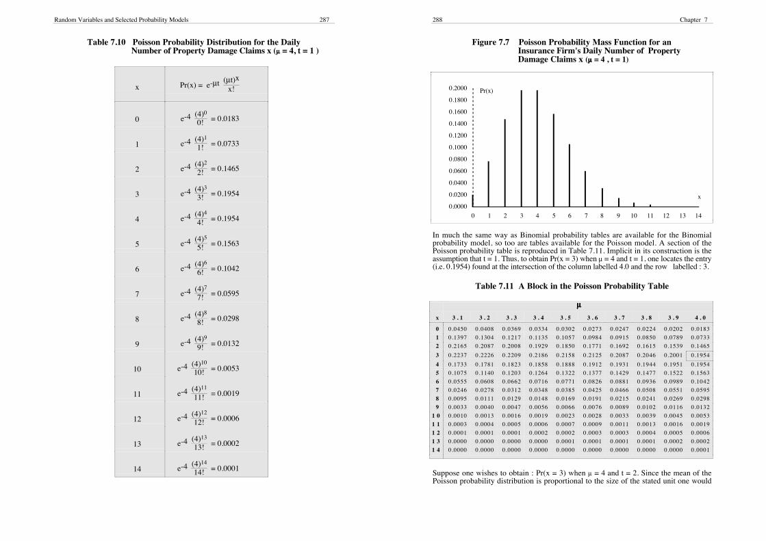
Table 7.10 Poisson Probability Distribution for the DailyNumber of Property Damage Claims x (µµµµ = 4, t = 1 )
x Pr(x) = e-µt (µt)x
x!
0 e-4 (4)0
0! = 0.0183
1 e-4 (4)1
1! = 0.0733
2 e-4 (4)2
2! = 0.1465
3 e-4 (4)3
3! = 0.1954
4 e-4 (4)4
4! = 0.1954
5 e-4 (4)5
5! = 0.1563
6 e-4 (4)6
6! = 0.1042
7 e-4 (4)7
7! = 0.0595
8 e-4 (4)8
8! = 0.0298
9 e-4 (4)9
9! = 0.0132
10 e-4 (4)10
10! = 0.0053
11 e-4 (4)11
11! = 0.0019
12 e-4 (4)12
12! = 0.0006
13 e-4 (4)13
13! = 0.0002
14 e-4 (4)14
14! = 0.0001
288 Chapter 7
Figure 7.7 Poisson Probability Mass Function for anInsurance Firm's Daily Number of PropertyDamage Claims x (µµµµ = 4 , t = 1)
0.0000
0.0200
0.0400
0.0600
0.0800
0.1000
0.1200
0.1400
0.1600
0.1800
0.2000
0 1 2 3 4 5 6 7 8 9 10 11 12 13 14
Pr(x)
x
In much the same way as Binomial probability tables are available for the Binomialprobability model, so too are tables available for the Poisson model. A section of thePoisson probability table is reproduced in Table 7.11. Implicit in its construction is theassumption that t = 1. Thus, to obtain Pr(x = 3) when µ = 4 and t = 1, one locates the entry(i.e. 0.1954) found at the intersection of the column labelled 4.0 and the row labelled : 3.
Table 7.11 A Block in the Poisson Probability Table
µµµµx 3 . 1 3 . 2 3 . 3 3 . 4 3 . 5 3 . 6 3 . 7 3 . 8 3 . 9 4 . 0
0 0.0450 0.0408 0.0369 0.0334 0.0302 0.0273 0.0247 0.0224 0.0202 0.0183
1 0.1397 0.1304 0.1217 0.1135 0.1057 0.0984 0.0915 0.0850 0.0789 0.0733
2 0.2165 0.2087 0.2008 0.1929 0.1850 0.1771 0.1692 0.1615 0.1539 0.1465
3 0.2237 0.2226 0.2209 0.2186 0.2158 0.2125 0.2087 0.2046 0.2001 0.1954
4 0.1733 0.1781 0.1823 0.1858 0.1888 0.1912 0.1931 0.1944 0.1951 0.1954
5 0.1075 0.1140 0.1203 0.1264 0.1322 0.1377 0.1429 0.1477 0.1522 0.1563
6 0.0555 0.0608 0.0662 0.0716 0.0771 0.0826 0.0881 0.0936 0.0989 0.1042
7 0.0246 0.0278 0.0312 0.0348 0.0385 0.0425 0.0466 0.0508 0.0551 0.0595
8 0.0095 0.0111 0.0129 0.0148 0.0169 0.0191 0.0215 0.0241 0.0269 0.0298
9 0.0033 0.0040 0.0047 0.0056 0.0066 0.0076 0.0089 0.0102 0.0116 0.0132
1 0 0.0010 0.0013 0.0016 0.0019 0.0023 0.0028 0.0033 0.0039 0.0045 0.0053
1 1 0.0003 0.0004 0.0005 0.0006 0.0007 0.0009 0.0011 0.0013 0.0016 0.0019
1 2 0.0001 0.0001 0.0001 0.0002 0.0002 0.0003 0.0003 0.0004 0.0005 0.0006
1 3 0.0000 0.0000 0.0000 0.0000 0.0001 0.0001 0.0001 0.0001 0.0002 0.0002
1 4 0.0000 0.0000 0.0000 0.0000 0.0000 0.0000 0.0000 0.0000 0.0000 0.0001
Suppose one wishes to obtain : Pr(x = 3) when µ = 4 and t = 2. Since the mean of thePoisson probability distribution is proportional to the size of the stated unit one would
Random Variables and Selected Probability Models 289
look for the entry (i.e. 0.0286) found at the intersection of the row labelled : 3 and thecolumn labelled : 8 (i.e. µt = 2x4). This entry is indicated in Table 7.12 below :
Table 7.12 Another Block in the Poisson Probability Table
µµµµ
x 7 . 1 7 . 2 7 . 3 7 . 4 7 . 5 7 . 6 7 . 7 7 . 8 7 . 9 8 . 0
0 0.0008 0.0007 0.0007 0.0006 0.0006 0.0005 0.0005 0.0004 0.0004 0.00031 0.0059 0.0054 0.0049 0.0045 0.0041 0.0038 0.0035 0.0032 0.0029 0.00272 0.0208 0.0194 0.0180 0.0167 0.0156 0.0145 0.0134 0.0125 0.0116 0.01073 0.0492 0.0464 0.0438 0.0413 0.0389 0.0366 0.0345 0.0324 0.0305 0.02864 0.0874 0.0836 0.0799 0.0764 0.0729 0.0696 0.0663 0.0632 0.0602 0.05735 0.1241 0.1204 0.1167 0.1130 0.1094 0.1057 0.1021 0.0986 0.0951 0.09166 0.1468 0.1445 0.1420 0.1394 0.1367 0.1339 0.1311 0.1282 0.1252 0.12217 0.1489 0.1486 0.1481 0.1474 0.1465 0.1454 0.1442 0.1428 0.1413 0.13968 0.1321 0.1337 0.1351 0.1363 0.1373 0.1381 0.1388 0.1392 0.1395 0.13969 0.1042 0.1070 0.1096 0.1121 0.1144 0.1167 0.1187 0.1207 0.1224 0.1241
1 0 0.0740 0.0770 0.0800 0.0829 0.0858 0.0887 0.0914 0.0941 0.0967 0.09931 1 0.0478 0.0504 0.0531 0.0558 0.0585 0.0613 0.0640 0.0667 0.0695 0.07221 2 0.0283 0.0303 0.0323 0.0344 0.0366 0.0388 0.0411 0.0434 0.0457 0.04811 3 0.0154 0.0168 0.0181 0.0196 0.0211 0.0227 0.0243 0.0260 0.0278 0.02961 4 0.0078 0.0086 0.0095 0.0104 0.0113 0.0123 0.0134 0.0145 0.0157 0.01691 5 0.0037 0.0041 0.0046 0.0051 0.0057 0.0062 0.0069 0.0075 0.0083 0.00901 6 0.0016 0.0019 0.0021 0.0024 0.0026 0.0030 0.0033 0.0037 0.0041 0.00451 7 0.0007 0.0008 0.0009 0.0010 0.0012 0.0013 0.0015 0.0017 0.0019 0.00211 8 0.0003 0.0003 0.0004 0.0004 0.0005 0.0006 0.0006 0.0007 0.0008 0.00091 9 0.0001 0.0001 0.0001 0.0002 0.0002 0.0002 0.0003 0.0003 0.0003 0.00042 0 0.0000 0.0000 0.0001 0.0001 0.0001 0.0001 0.0001 0.0001 0.0001 0.00022 1 0.0000 0.0000 0.0000 0.0000 0.0000 0.0000 0.0000 0.0000 0.0001 0.0001
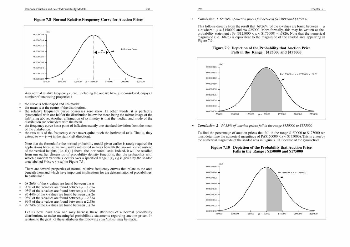
A table of cumulative probabilities is also available for the Poisson distribution. A blockfrom this table is reproduced in Table 7.13. We may illustrate its use by supposing wewish to find the probability that there are 3 or less property damage claims when the dailyaverage number of property claims is 4. Then, this probability [i.e. Pr(x ≤ 3) = .4335] isfound at the intersection of the row labelled : x = 3 and the column labelled : µ = 4.0 inTable 7.13.
We may also use this table to find a probability like : Pr(x > 3). In the present context thisis the probability that the daily number of property claims is greater than 3. But :
Pr(x ≤ 3) + Pr(x > 3) = 1 ⇒ Pr(x > 3) = 1 - Pr(x ≤ 3) = 1 - .4335 = 0.5665
We end this section with a brief comment on the expected value and variance of thePoisson probability distribution. These are respectively given by :
E(x) = µt and V(x) = µt
where µ and t are defined as earlier. Let us now return to our example which revolvesaround property damage claims. Then :
E(x) = 4 claims and V(x) = 4 claims2 when µ = 4 and t = 1
E(x) = 8 claims and V(x) = 8 claims2 when µ = 4 and t = 2
290 Chapter 7
Table 7.13 A Section of the Cumulative Poisson Probability Table
µµµµ
x 3 . 1 3 . 2 3 . 3 3 . 4 3 . 5 3 . 6 3 . 7 3 . 8 3 . 9 4 . 0
0 0.0450 0.0408 0.0369 0.0334 0.0302 0.0273 0.0247 0.0224 0.0202 0.01831 0.1847 0.1712 0.1586 0.1468 0.1359 0.1257 0.1162 0.1074 0.0992 0.0916
2 0.4012 0.3799 0.3594 0.3397 0.3208 0.3027 0.2854 0.2689 0.2531 0.2381
3 0.6248 0.6025 0.5803 0.5584 0.5366 0.5152 0.4942 0.4735 0.4532 0.4335
4 0.7982 0.7806 0.7626 0.7442 0.7254 0.7064 0.6872 0.6678 0.6484 0.6288
5 0.9057 0.8946 0.8829 0.8705 0.8576 0.8441 0.8301 0.8156 0.8006 0.7851
6 0.9612 0.9554 0.9490 0.9421 0.9347 0.9267 0.9182 0.9091 0.8995 0.8893
7 0.9858 0.9832 0.9802 0.9769 0.9733 0.9692 0.9648 0.9599 0.9546 0.9489
8 0.9953 0.9943 0.9931 0.9917 0.9901 0.9883 0.9863 0.9840 0.9815 0.9786
9 0.9986 0.9982 0.9978 0.9973 0.9967 0.9960 0.9952 0.9942 0.9931 0.9919
1 0 0.9996 0.9995 0.9994 0.9992 0.9990 0.9987 0.9984 0.9981 0.9977 0.9972
1 1 0.9999 0.9999 0.9998 0.9998 0.9997 0.9996 0.9995 0.9994 0.9993 0.9991
1 2 1.0000 1.0000 1.0000 0.9999 0.9999 0.9999 0.9999 0.9998 0.9998 0.9997
1 3 1.0000 1.0000 1.0000 1.0000 1.0000 1.0000 1.0000 1.0000 0.9999 0.9999
1 4 1.0000 1.0000 1.0000 1.0000 1.0000 1.0000 1.0000 1.0000 1.0000 1.0000
The Normal (or Gaussian) Probability Distribution
Perhaps the most important and most widely used probability model in statistics is thenormal or Gaussian probability model 7. However, unlike the Poisson and Binomialprobability models, the normal probability model is one that is applicable to a continuousrandom variable x. The general mathematical form of the relative frequency curveassociated with the normal distribution is given by the following expression.
f(x) = 1
σ√⎯⎯2π e
12 (x - µ ) 2 /σ2-
where the mean and standard deviation of the distribution are given by µ and σ respectivelyand π = 3.14159 .... and e = 2.71828 .....
We may illustrate the idea of such a distribution by assuming metropolitan auction pricesare normally distributed with a mean µ = $150000 and a standard deviation σ = $25000.Then, f(x) would be given by :
f(x) = 1
25000√⎯⎯2π e
12 ( x - ) 2/2
150000 25000-
Moreover, when f(x) is graphed against x we obtain the relative frequency curve in Figure7.8.
7 The Gaussian probability distribution is named after Karl Gauss (1777 - 1855) who was the bestknown of several mathematicians that contributed to its formulation. Other originators includeAbraham De Moivre (1667 - 1754) and Pierre Laplace (1749 - 1827).
Random Variables and Selected Probability Models 291
Figure 7.8 Normal Relative Frequency Curve for Auction Prices
0.000000
0.000002
0.000004
0.000006
0.000008
0.000010
0.000012
0.000014
0.000016
75000 100000 125000 150000 175000 200000 225000
f(x)
σ Inflexion Point
µ =
Any normal relative frequency curve, including the one we have just considered, enjoys anumber of interesting properties :
• the curve is bell-shaped and uni-modal• the mean is at the centre of the distribution.• the relative frequency curve possesses zero skew. In other words, it is perfectly
symmetrical with one half of the distribution below the mean being the mirror image of thehalf lying above. Another affirmation of symmetry is that the median and mode of thedistribution are coincident with the mean.
• the frequency curve has a point of inflexion exactly one standard deviation from the meanof the distribution.
• the two tails of the frequency curve never quite touch the horizontal axis. That is, theyextend to + ∞ (- ∞) in the right (left direction).
Note that the formula for the normal probability model given earlier is rarely required forapplications because we are usually interested in areas beneath the normal curve insteadof the vertical heights [ i.e. f(x) ] above the horizontal axis. Indeed, it will be recalledfrom our earlier discussion of probability density functions, that the probability withwhich a random variable x occurs over a specified range : (xa xb) is given by the shadedarea labelled Pr(xa < x < xb) in Figure 7.5.
There are several properties of normal relative frequency curves that relate to the areabeneath them and which have important implications for the determination of probabilities.In particular :
• 68.26% of the x-values are found between µ ± σ• 90% of the x-values are found between µ ± 1.65σ• 95% of the x-values are found between µ ± 1.96σ• 95.44% of the x-values are found between µ ± 2σ• 98% of the x-values are found between µ ± 2.33σ• 99% of the x-values are found between µ ± 2.58σ• 99.74% of the x-values are found between µ ± 3σ
Let us now learn how one may harness these attributes of a normal probabilitydistribution, to make meaningful probabilistic statements regarding auction prices. Inrelation to the first of these attributes the following conclusions may be made.
292 Chapter 7
• Conclusion 1 68.26% of auction prices fall between $125000 and $175000.
This follows directly from the result that 68.26% of the x-values are found between µ± σ where : µ = $150000 and σ = $25000. More formally, this may be written as theprobability statement : Pr ($125000 < x < $175000) = .6826. Note that the numericalmagnitude (i.e. .6826) is equivalent to the magnitude of the shaded area appearing inFigure 7.9.
Figure 7.9 Depiction of the Probability that Auction PriceFalls in the Range : $125000 and $175000
0.000000
0.000002
0.000004
0.000006
0.000008
0.000010
0.000012
0.000014
0.000016
75000 100000 125000 150000 175000 200000 225000
f(x)
µ =
Pr(125000 < x < 175000) = .6826
• Conclusion 2 34.13% of auction prices fall in the range $150000 to $175000
To find the percentage of auction prices that fall in the range $150000 to $175000 wemust determine the numerical magnitude of Pr($150000 < x < $175000). This is given bythe numerical magnitude of the shaded area in Figure 7.10. Because of the symmetrical
Figure 7.10 Depiction of the Probability that Auction PriceFalls in the Range : $150000 and $175000
0.000000
0.000002
0.000004
0.000006
0.000008
0.000010
0.000012
0.000014
0.000016
75000 100000 125000 150000 175000 200000 225000
f(x)
µ =
Pr(150000 < x < 175000)
Random Variables and Selected Probability Models 293
properties of the normal probability distribution, it follows that Pr($125000 < x <$175000) will be half of the area depicted in Figure 7.9. Since the shaded area in Figure7.9 came to .6826 it follows that the shaded area in Figure 7.10 is .5(.6826) = .3413 or34.13%.
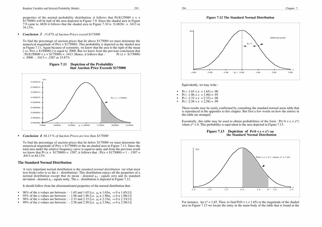
• Conclusion 3 15.87% of Auction Prices exceed $175000
To find the percentage of auction prices that lie above $175000 we must determine thenumerical magnitude of Pr(x > $175000). This probability is depicted as the shaded areain Figure 7.11. Again because of symmetry, we know that the area to the right of the mean[ i.e. Pr(x > $150000) ] is equal to .5000. But we know from the previous conclusion that: Pr($150000 < x < $175000) = .3413. Hence, it follows that : Pr (x > $175000)= .5000 - .3413 = .1587 or 15.87%
Figure 7.11 Depiction of the Probabilitythat Auction Price Exceeds $175000
0.000000
0.000002
0.000004
0.000006
0.000008
0.000010
0.000012
0.000014
0.000016
75000 100000 125000 150000 175000 200000 225000
f(x)
µ =
Pr( x > 175000)
• Conclusion 4 84.13 % of Auction Prices are less than $175000
To find the percentage of auction prices that lie below $175000 we must determine thenumerical magnitude of Pr(x < $175000) or the un-shaded area in Figure 7.11. Since thetotal area under the relative frequency curve is equal to unity and from the previous resultwe know that Pr (x > $175000) = .1587, it follows that : Pr(x < $175000) = 1 - .1587 =.8413 or 84.13%
The Standard Normal Distribution
A very important normal distribution is the standard normal distribution (or what mosttext books refer to as the z - distribution). This distribution enjoys all the properties of anormal distribution except that its mean - denoted µz - equals zero and its standarddeviation - denoted σz - equals unity. The z - distribution is depicted in Figure 7.12.
It should follow from the aforementioned properties of the normal distribution that :
• 90% of the z-values are between : - 1.65 and 1.65 [i.e. µz ± 1.65σz ⇒ 0 ± 1.65(1)]• 95% of the z-values are between : - 1.96 and 1.96 [i.e. µz ± 1.96σz ⇒ 0 ± 1.96(1)]• 98% of the z-values are between : - 2.33 and 2.33 [i.e. µz ± 2.33σz ⇒ 0 ± 2.33(1)]• 99% of the z-values are between : - 2.58 and 2.58 [i.e. µz ± 2.58σz ⇒ 0 ± 2.58(1)]
294 Chapter 7
Figure 7.12 The Standard Normal Distribution
f(z)
-3.00 -2.00 -1.00 0.00 1.00 2.00 3.00µ =z
z
Inflexion point
σ = 1z
Equivalently, we may write :
• Pr ( -1.65 < z < 1.65) = .90• Pr ( -1.96 < z < 1.96) = .95• Pr ( -2.33 < z < 2.33) = .98• Pr ( -2.58 < z < 2.58) = .99
These results may be easily confirmed by consulting the standard normal areas table thatis reproduced in the appendix to this chapter. But first a few words on how the entries inthis table are arranged.
Essentially, this table may be used to obtain probabilities of the form : Pr( 0 < z < z*)where z* > 0. This probability is equivalent to the area depicted in Figure 7.13.
Figure 7.13 Depiction of Pr(0 < z < z*) onthe Standard Normal Distribution
f(z)
-3.0 -2.0 -1.0 0.0 1.0 2.0 3.0z
Pr(0 < z < z*) where z* = 1.65
z*
For instance, let z* = 1.65. Then, to find Pr(0 < z < 1.65) or the magnitude of the shadedarea in Figure 7.13 we locate the entry in the main body of the table that is found at the
Random Variables and Selected Probability Models 295
intersection of the row labelled : 1.60 and the column labelled .05. It should be clear bynow that the row and column headings of the standard normal areas table effectivelyidentify the z*-value (i.e. z* = 1.60 + .05 = 1.65). Now the entry at the intersectionpoint is found to be .4505. Moreover, since the standard normal distribution issymmetrical it follows that :
Pr(-1.65 < z < 1.65) = 2 × Pr(0 < z < 1.65) = 2 × (.4505) ≅ .90 or 90%
which confirms our earlier cited result. The keen reader should try to use the areas table toconfirm remaining probabilistic properties (cited earlier) of the standard normaldistribution.
There is only one table of areas available for normal distributions - the one that relates tothe standard normal distribution. Does this mean that we are restricted to the resolution ofproblems in which the variable of interest is standard normally distributed? The answer tothis question is 'yes' as well as 'no'.
We may say 'yes', because strictly speaking the table of areas relates to a standard normaldistribution alone. On the other hand, we may say 'no', because every normally distributedvariable x may be converted into a standard normally distributed variable z by applying thefollowing data transformation :
z = x - µ
σ
where : z measures in standard deviation units how far above or below the mean an actualx-value lies. Thus, if we standardize each of the x-values - i.e. compute corresponding z-values - the resultant distribution of z-values will be standard normally distributed. Thisexceedingly important result, enables us to convert any problem relating to a normaldistribution into a similar problem that relates to the standard normal distribution. And, forthis reason, only one table of areas is required to address any problem that initially relatesto a normal rather than standard normal distribution. Having described the nature of thestandard normal distribution, let us now use a series of worked problems to explore moredeeply how the z-distribution may be used to address typical questions relating to anormally distributed variable x.
In each of the worked problems appearing below we make use of earlier example ofnormally distributed auction prices.
• Worked Problem 1
Determine the probability that auction price lies between $158000 and $179000 if meanauction price equals $150000 with a standard deviation of $25000 .
Symbolically, we are required to obtain : Pr(x1 < x < x2) where : x1 = $158000 and x2= $179000. To solve this problem, one must first transform (or standardize) x1 and x2into the values : z1 and z2 respectively. This is done immediately below :
z1 = x1 - µ
σ = [$158000 - $150000]
$25000 = .32 and
z2 = x2 - µ
σ = [$179000 - $150000]
$25000 = 1.16
But Pr(z1 < z < z2) = Pr(x1 < x < x2).
So, we may use the standard normal area tables to find Pr(.32 < z < 1.16) which will beequivalent to determining Pr($158000 < x < $179000), our initially stated objective.
296 Chapter 7
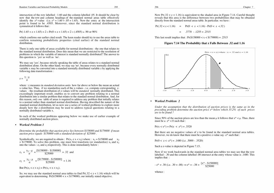
Now Pr(.32 < z < 1.16) is equivalent to the shaded area in Figure 7.14. Careful thoughtreveals that this area is the difference between two probabilities that may be obtaineddirectly from the standard normal areas table. In particular, we have :
Pr(.32 < z < 1.16) = Pr(0 < z < 1.16) - Pr(0 < z <.32 )
= .3770 - .1255 = .2515
This last result implies that : Pr($158000 < x < $179000) = .2515
Figure 7.14 The Probability that z Falls Between .32 and 1.16
f(z)
-3.0 -2.0 -1.0 0.0 1.0 2.0 3.0zz1 z2
Pr(z1 < z < z2) where : z1 = .32 and z2 = 1.16
• Worked Problem 2
Under the assumption that the distribution of auction prices is the same as in thepreceding problem determine the auction price x* below which 35.2% of such pricesare to be found ?
Since 50% of the auction prices are less than the mean µ it follows that x* < µ. Thus, theremust be a z* < 0 such that :
Pr(x < x*) = Pr(z < z*) = .3520
But there are no negative values of z to be found in the standard normal area tables.However, we do know that there must be a positive z-value say -z* such that :
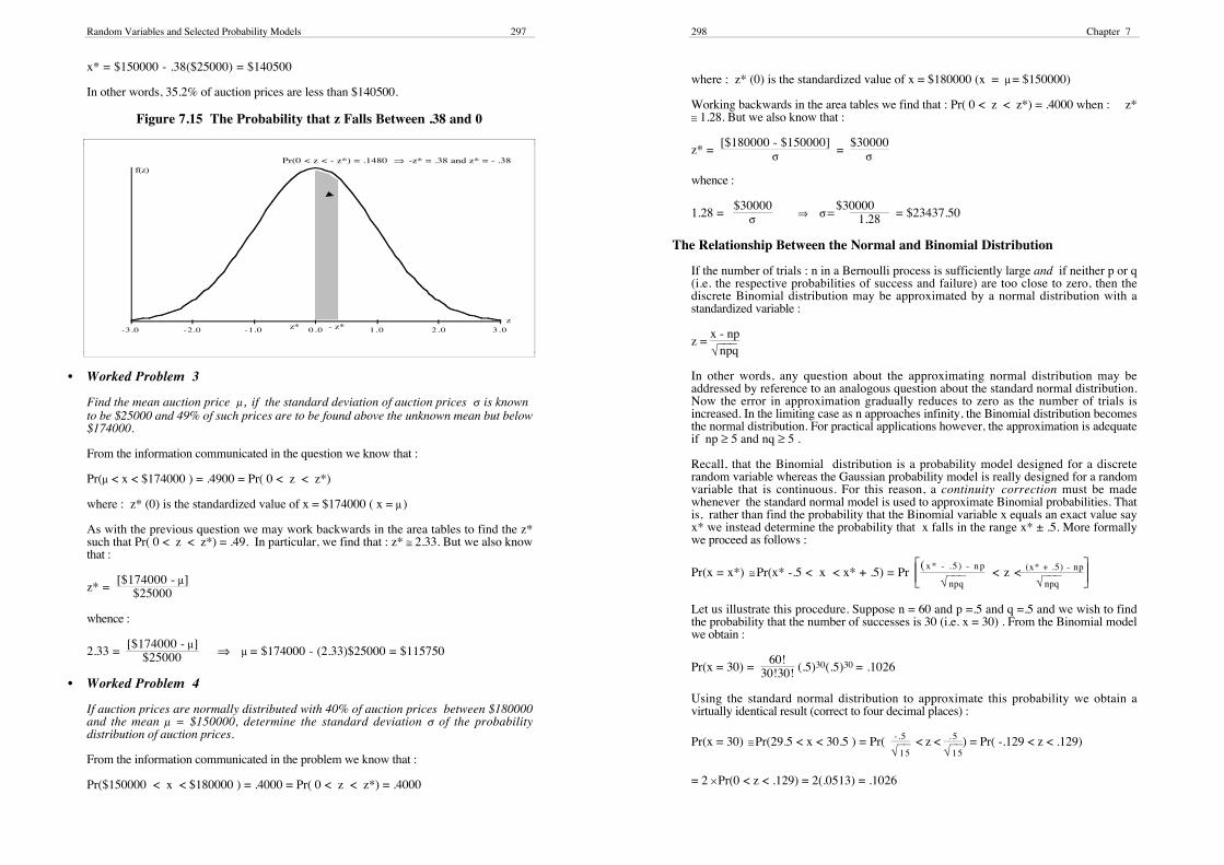
Pr(0 < z < -z*) = .1480 (i.e. .5000 - .3520)
Such a z-value is depicted in Figure 7.15.
Now if we work backwards in the standard normal area tables we may see that the rowlabelled : .30 and the column labelled .08 intersect at the entry whose value is .1480. Thisimplies that :
- z* = .38 (i.e. .30 + .08) ⇒ z* = -.38 = [x* - $150000]
$25000
whence :
Random Variables and Selected Probability Models 297
x* = $150000 - .38($25000) = $140500
In other words, 35.2% of auction prices are less than $140500.
Figure 7.15 The Probability that z Falls Between .38 and 0
f(z)
-3.0 -2.0 -1.0 0.0 1.0 2.0 3.0z
- z*z*
Pr(0 < z < - z*) = .1480 ⇒ -z* = .38 and z* = - .38
• Worked Problem 3
Find the mean auction price µ , if the standard deviation of auction prices σ is knownto be $25000 and 49% of such prices are to be found above the unknown mean but below$174000.
From the information communicated in the question we know that :
Pr(µ < x < $174000 ) = .4900 = Pr( 0 < z < z*)
where : z* (0) is the standardized value of x = $174000 ( x = µ )
As with the previous question we may work backwards in the area tables to find the z*such that Pr( 0 < z < z*) = .49. In particular, we find that : z* ≅ 2.33. But we also knowthat :
z* = [$174000 - µ]
$25000
whence :
2.33 = [$174000 - µ]
$25000 ⇒ µ = $174000 - (2.33)$25000 = $115750
• Worked Problem 4
If auction prices are normally distributed with 40% of auction prices between $180000and the mean µ = $150000, determine the standard deviation σ of the probabilitydistribution of auction prices.
From the information communicated in the problem we know that :
Pr($150000 < x < $180000 ) = .4000 = Pr( 0 < z < z*) = .4000
298 Chapter 7
where : z* (0) is the standardized value of x = $180000 (x = µ = $150000)
Working backwards in the area tables we find that : Pr( 0 < z < z*) = .4000 when : z*≅ 1.28. But we also know that :
z* = [$180000 - $150000]
σ = $30000
σ
whence :
1.28 = $30000
σ ⇒ σ = $300001.28 = $23437.50
The Relationship Between the Normal and Binomial Distribution
If the number of trials : n in a Bernoulli process is sufficiently large and if neither p or q(i.e. the respective probabilities of success and failure) are too close to zero, then thediscrete Binomial distribution may be approximated by a normal distribution with astandardized variable :
z = x - np
√⎯⎯⎯npq
In other words, any question about the approximating normal distribution may beaddressed by reference to an analogous question about the standard normal distribution.Now the error in approximation gradually reduces to zero as the number of trials isincreased. In the limiting case as n approaches infinity, the Binomial distribution becomesthe normal distribution. For practical applications however, the approximation is adequateif np ≥ 5 and nq ≥ 5 .
Recall, that the Binomial distribution is a probability model designed for a discreterandom variable whereas the Gaussian probability model is really designed for a randomvariable that is continuous. For this reason, a continuity correction must be madewhenever the standard normal model is used to approximate Binomial probabilities. Thatis, rather than find the probability that the Binomial variable x equals an exact value sayx* we instead determine the probability that x falls in the range x* ± .5. More formallywe proceed as follows :
Pr(x = x*) ≅ Pr(x* -.5 < x < x* + .5) = Pr ⎣⎢⎢⎡
⎦⎥⎥⎤(x* - . 5 ) - np
√⎯⎯⎯npq < z < (x* + .5) - np
√⎯⎯⎯npq
Let us illustrate this procedure. Suppose n = 60 and p =.5 and q =.5 and we wish to findthe probability that the number of successes is 30 (i.e. x = 30) . From the Binomial modelwe obtain :
Pr(x = 30) = 60!
30!30! (.5)30(.5)30 = .1026
Using the standard normal distribution to approximate this probability we obtain avirtually identical result (correct to four decimal places) :
Pr(x = 30) ≅ Pr(29.5 < x < 30.5 ) = Pr( -.5
√⎯⎯15 < z < . 5
√⎯⎯15) = Pr( -.129 < z < .129)
= 2 × Pr(0 < z < .129) = 2(.0513) = .1026
Random Variables and Selected Probability Models 299
A more general application of the principle of continuity correction occurs when we seekto approximate : Pr(x1 ≤ x ≤ x2) where : x1 and x2 respectively denote the inclusivelower and upper bound of the range within which the Binomial variable x is located forthe purposes of the probability calculation. Here the continuity correction manifests itselfin the following manner :
Pr(x1 ≤ x ≤ x2) ≅ Pr(x1 -.5 < x < x2 +.5 ) = Pr ⎣⎢⎢⎡
⎦⎥⎥⎤(x 1 - . 5 ) - np
√⎯⎯⎯npq < z <
(x2 + .5) - np
√⎯⎯⎯npq
Let us now illustrate the accuracy of the approximation for Pr(30 ≤ x ≤ 31). If we retainour previous assumptions for p, q and n, then the Binomial model will yield the followingresult :
Pr(30 ≤ x ≤ 31) = Pr(x = 30) + Pr(x = 31) = 60!30!30! (.5)30(.5)30 + 60!
31!29! (.5)31(.5)29
= .1026 + .0993 = 0.2019
If we now employ the standard normal distribution to approximate this probability weobtain the same result (correct to four decimal places).
Pr(30 ≤ x ≤ 31) ≅ Pr(30 - .5 < x < 31 + .5 ) = Pr ⎣⎢⎢⎡
⎦⎥⎥⎤(30 - . 5 ) - 30
√⎯⎯15 < z < (31 + .5) - 30
√⎯⎯15
= Pr(-.129 < z < .387) = Pr(0 < z < .129) + Pr (0 < z < .387)
= .0513 + .1506 = 0.2019
The Relationship Between the Binomial and Poisson Distribution
It may be shown, though not here, that if the number of trials of a Bernoulli processapproaches infinity and the probability of success : p at each trial approaches zero then theBinomial distribution collapses into the Poisson distribution. More importantly forpractical applications, if the number of trials : n ≥ 50 and if np < 5, then the Binomialdistribution may be reasonably approximated by the Poisson distribution with µ = np andt = 1.
Consider the following case in which n ≥ 50 and np < 5 :
n = 150 p = .01 and q =.99 [ ⇒ n > 50 and np = 1.5 < 5]
Now let us compute Pr(x=1) using the Binomial and Poisson probability models andgauge the difference in computed values. Using the Binomial model we obtain :
Pr(x = 1) = n!
(n-x)! x! (p)x(q)n-x = 150!
149!1! (.01)1(.99)149 = .3355
and if we use the Poisson Probability model (with t = 1 and µ = np) as an approximationwe obtain :
Pr(x = 1) ≅ e- µ t (µt)x
x! = e- 1.5 (1.5)1
1! =.3347
This represents an approximation error of between one fifth and one quarter of onepercent.
300 Chapter 7
The Relationship Between the Poisson and Normal Distribution
It may be shown that as µ - the mean number of occurrences per stated unit - increasesindefinitely, that a Poisson distribution approaches a normal distribution with astandardized variable :
z = (x - µ)
√⎯ µ
7.3 Use of the HP-10B and EXCEL
In this section we demonstrate how EXCEL and the HP-10B may be used to performtasks that are related to the material covered earlier in this chapter.
Using the HP - 10B to Compute Expected Values
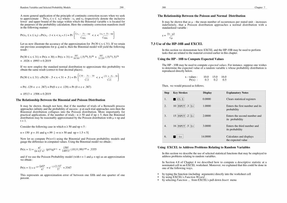
The HP - 10B may be used to compute expected values. For instance, suppose one wishesto determine the expected value of a random variable x whose probability distribution isreproduced directly below.
x - values : 10.0 15.0 16.0Pr(x) : 0.3 0.2 0.5
Then, we would proceed as follows.
Step Key Strokes Display Explanatory Notes
1. ■ CL Σ 0.0000 Clears statistical registers
2. 10 INPUT .3 Σ+ 1.0000 Enters the first number and its probability
3. 15 INPUT .2 Σ+ 2.0000 Enters the second number and its probability
4. 16 INPUT .5 Σ+ 3.0000 Enters the third number and its probability
6. ■ -xw 14.0000 Calculates and displaysthe expected value
Using EXCEL to Address Problems Relating to Random Variables
In this section we describe the use of selected statistical functions that may be employed toaddress problems relating to random variables.
In Section 4.8 of Chapter 4 we described how to compute a descriptive statistic at anominated cell in an EXCEL worksheet. Moreover, we explained that this could be done inone of the following ways.
• by typing the function (including arguments) directly into the worksheet cell• by using EXCEL's Function Wizard .• by selecting Function ... from EXCEL's pull down Insert menu
Random Variables and Selected Probability Models 301
All of these approaches apply to the statistical functions which we describe immediatelybelow.
The BINOMDIST Function
The BINOMDIST function is designed to return Binomial probabilities. The syntax forthis function is given by =BINOMDIST(x, n , p, cumulative).
Here the argument x denotes the number of successes, n denotes the number of trials andp denotes the probability of a success at each trial. Finally, the argument labelledcumulative denotes a logical value that is set to false (true) if one wishes to return the(cumulative) probability that x (x or less) occurs.
For example, consider a fair coin that is tossed 10 times. Then, the probability that the coincomes up heads 4 out of 10 times is given by :
Pr(x = 4) =BINOMDIST(4, 10, .5, false) = 0.2050
Moreover, the probability that 4 or less heads come up is given by :
Pr(x ≤ 4) =BINOMDIST(4, 10, .5, true) = 0.3770
The POISSON Function
As its name suggests, the POISSON function is designed to return Poisson probabilities.The syntax for this function is given by =POISSON(x, µ, cumulative).
Here the argument x denotes the number of times a specified event occurs per stated unitand µ denotes the mean number of occurrences per stated unit. Finally, the argument thatis labelled cumulative has the same interpretation as the argument of the same name in theBINOMDIST function.
As an example, suppose we wish to determine the probability that 3 property insuranceclaims are made over a day when the average number of daily claims is 2. Then, thearguments of the POISSON function would be inserted as follows :
Pr(x = 3) =POISSON(3, 2, false) = 0.1804
On the other hand, if we wish to compute the probability that 3 or less property insuranceclaims are made over a day, then we would employ the arguments displayed below.
Pr(x ≤ 3) =POISSON(3, 2, true) = 0.8571
The NORMDIST and NORMINV Functions
The NORMDIST function is designed to return Gaussian probabilities. The syntax forthis function is given by =NORMDIST(x, µ, σ, cumulative).
Here the x argument represents the particular value of a normally distributed variable atwhich the NORMDIST function is to be evaluated. Moreover, µ and σ respectively denotethe mean and standard deviation of the normally distributed variable. Finally, the argumentthat is labelled cumulative has much the same interpretation as the identically labelledargument appearing in the BINOMDIST function.
As an example, suppose auction prices are normally distributed with a mean of 150000and a standard deviation of 25000. Then, the probability that an auction price x is lessthan 175000 is given by :Pr(x < 175000) =NORMDIST(175000, 150000, 25000, true) = 0.8413
302 Chapter 7
Moreover, the probability that auction price is between $175000 and the mean auctionprice of 150000 is given by :
Pr(150000 < x < 175000) =NORMDIST(175000, 150000, 25000, true) - .5 = 0.3413
Suppose we now wish to find the vertical height of the bell shaped Gaussian probabilitydistribution (Note, this is not a probability) at an auction price of 175000. Then, thiswould be given by :
=NORMDIST(175000, 150000, 25000, false) = 0.0584.
Careful thought reveals that by setting the cumulative argument to false for a series ofdifferent x-values (i.e. auction prices) and then plotting as a line graph the resultantNORMDIST values against their corresponding x-values, we are able to trace out the bell-shaped curve for this normally distributed variable.
The NORMINV function returns the inverse of the normal cumulative distribution for anominated mean and standard deviation. The syntax for this function is given byNORMINV(p, µ, σ). Here the p argument denotes cumulative probability with thearguments µ and σ possessing the same interpretation as identically labelled arguments inthe NORMDIST function.
As an example of this function, suppose we wish to determine the price beneath which areto be found 97.5% of the auction prices. If auction prices are normally distributed asdescribed earlier, we may use the NORMINV function as follows.
=NORMINV(.975, 150000, 25000) = 198999.03.
The NORMSDIST and NORMSINV Functions
The NORMSDIST function returns the standard normal cumulative distribution functionand may be used instead of a table of areas for the standard normal distribution. Thesyntax for the NORMSDIST function is given by =NORMSDIST(z) where theargument z is the value of the standardised variable for which the cumulative probability isto be determined.
As an example suppose we wish to determine the probability that the standard normalvariable is less than 1.96. Then, the NORMSDIST function would evaluate thisprobability as follows :
Pr(z < 1.96) = NORMSDIST(1.96) = 0.9750
Observe that this is not the same number that would be found if we looked up a z-value of1.96 in the standard normal areas table (reproduced in the appendix to this chapter). Thisis because the number in the areas table really represents Pr(0 < z < 1.96) = .4750 whichis equivalent to :
Pr(0 < z < 1.96) = NORMSDIST(1.96) - .5 = 0.4750
The NORMSINV function returns the inverse of the standard normal cumulativedistribution. In other words, this function returns the particular z-value below which is tobe found a nominated cumulative probability.
The syntax of the NORMSINV is given by =NORMSINV(p) where the argument pdenotes cumulative probability.
Random Variables and Selected Probability Models 303
As an example of this function suppose we wish to determine the z-value below which97.5% of z-values are to be found on a standard normal distribution. Then we wouldobtain our answer as follows :
=NORMSINV(.9750) = 1.96
The STANDARDIZE Function
The meaning of a standard random variable z, was defined in Remark 2 of this chapter(see Section 7.1). Now the STANDARDIZE function may be used to transform arandom variable x into a standardized random variable z.
The syntax for this function is given by =STANDARDIZE(x, µ, σ) where the x argumentis the value we wish to standardize and µ and σ are defined as in the NORMDISTfunction.
As an example of this function, suppose we wish to normalize the auction price of 175000when mean auction price is 150000 and its standard deviation is 25000. Then, ournormalised value is evaluated as follows :
=STANDARDIZE(175000, 150000, 25000) = 1.00 = 175000 - 150000
25000 = x - µ
σ = z
An Important Aside on EXCEL Functions for Random Variables
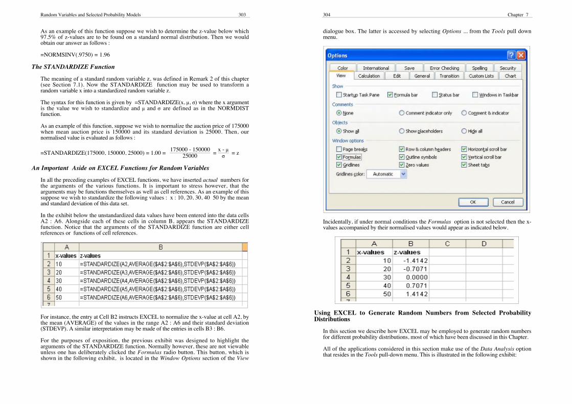
In all the preceding examples of EXCEL functions, we have inserted actual numbers forthe arguments of the various functions. It is important to stress however, that thearguments may be functions themselves as well as cell references. As an example of thissuppose we wish to standardize the following values : x : 10, 20, 30, 40 50 by the meanand standard deviation of this data set.
In the exhibit below the unstandardized data values have been entered into the data cellsA2 : A6. Alongside each of these cells in column B, appears the STANDARDIZEfunction. Notice that the arguments of the STANDARDIZE function are either cellreferences or functions of cell references.
For instance, the entry at Cell B2 instructs EXCEL to normalize the x-value at cell A2, bythe mean (AVERAGE) of the values in the range A2 : A6 and their standard deviation(STDEVP). A similar interpretation may be made of the entries in cells B3 : B6.
For the purposes of exposition, the previous exhibit was designed to highlight thearguments of the STANDARDIZE function. Normally however, these are not viewableunless one has deliberately clicked the Formulas radio button. This button, which isshown in the following exhibit, is located in the Window Options section of the View
304 Chapter 7
dialogue box. The latter is accessed by selecting Options ... from the Tools pull downmenu.
Incidentally, if under normal conditions the Formulas option is not selected then the x-values accompanied by their normalised values would appear as indicated below.
Using EXCEL to Generate Random Numbers from Selected ProbabilityDistributions
In this section we describe how EXCEL may be employed to generate random numbersfor different probability distributions, most of which have been discussed in this Chapter.
All of the applications considered in this section make use of the Data Analysis optionthat resides in the Tools pull-down menu. This is illustrated in the following exhibit:
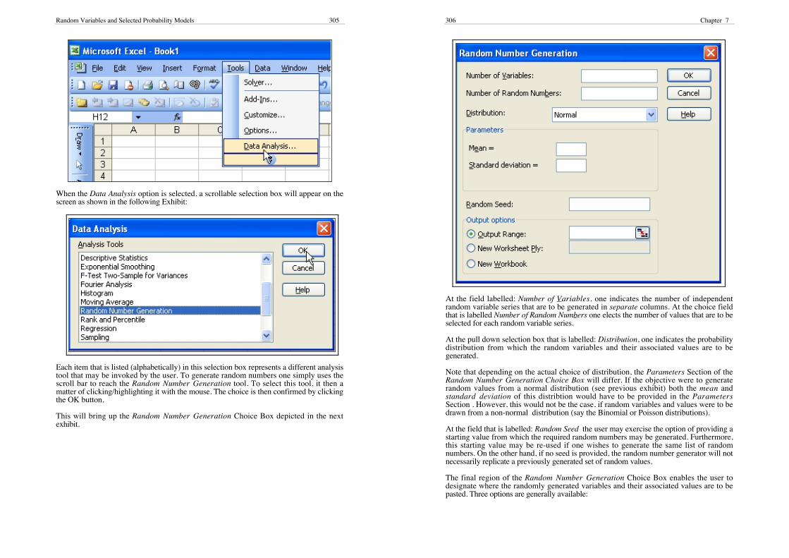
Random Variables and Selected Probability Models 305
When the Data Analysis option is selected, a scrollable selection box will appear on thescreen as shown in the following Exhibit:
Each item that is listed (alphabetically) in this selection box represents a different analysistool that may be invoked by the user. To generate random numbers one simply uses thescroll bar to reach the Random Number Generation tool. To select this tool, it then amatter of clicking/highlighting it with the mouse. The choice is then confirmed by clickingthe OK button.
This will bring up the Random Number Generation Choice Box depicted in the nextexhibit.
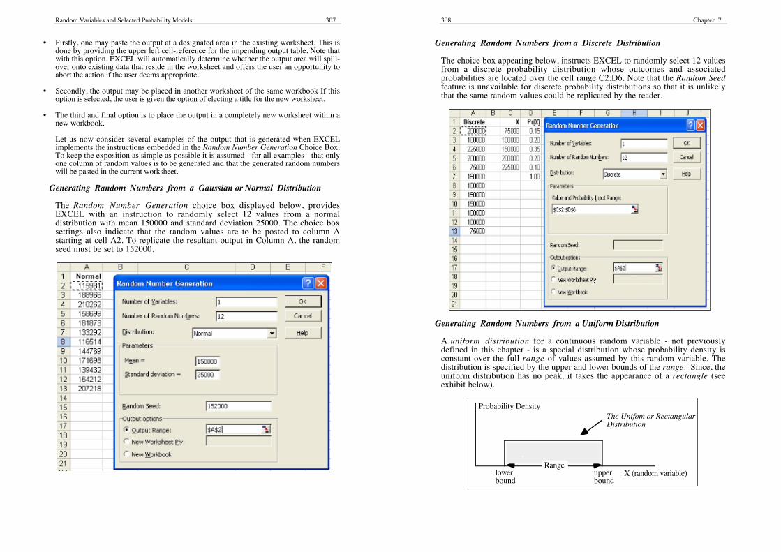
306 Chapter 7
At the field labelled: Number of Variables, one indicates the number of independentrandom variable series that are to be generated in separate columns. At the choice fieldthat is labelled Number of Random Numbers one elects the number of values that are to beselected for each random variable series.
At the pull down selection box that is labelled: Distribution, one indicates the probabilitydistribution from which the random variables and their associated values are to begenerated.
Note that depending on the actual choice of distribution, the Parameters Section of theRandom Number Generation Choice Box will differ. If the objective were to generaterandom values from a normal distribution (see previous exhibit) both the mean andstandard deviation of this distribtion would have to be provided in the ParametersSection . However, this would not be the case, if random variables and values were to bedrawn from a non-normal distribution (say the Binomial or Poisson distributions).
At the field that is labelled: Random Seed the user may exercise the option of providing astarting value from which the required random numbers may be generated. Furthermore,this starting value may be re-used if one wishes to generate the same list of randomnumbers. On the other hand, if no seed is provided, the random number generator will notnecessarily replicate a previously generated set of random values.
The final region of the Random Number Generation Choice Box enables the user todesignate where the randomly generated variables and their associated values are to bepasted. Three options are generally available:
Random Variables and Selected Probability Models 307
• Firstly, one may paste the output at a designated area in the existing worksheet. This isdone by providing the upper left cell-reference for the impending output table. Note thatwith this option, EXCEL will automatically determine whether the output area will spill-over onto existing data that reside in the worksheet and offers the user an opportunity toabort the action if the user deems appropriate.
• Secondly, the output may be placed in another worksheet of the same workbook If thisoption is selected, the user is given the option of electing a title for the new worksheet.
• The third and final option is to place the output in a completely new worksheet within anew workbook.
Let us now consider several examples of the output that is generated when EXCELimplements the instructions embedded in the Random Number Generation Choice Box.To keep the exposition as simple as possible it is assumed - for all examples - that onlyone column of random values is to be generated and that the generated random numberswill be pasted in the current worksheet.
Generating Random Numbers from a Gaussian or Normal Distribution
The Random Number Generation choice box displayed below, providesEXCEL with an instruction to randomly select 12 values from a normaldistribution with mean 150000 and standard deviation 25000. The choice boxsettings also indicate that the random values are to be posted to column Astarting at cell A2. To replicate the resultant output in Column A, the randomseed must be set to 152000.
308 Chapter 7
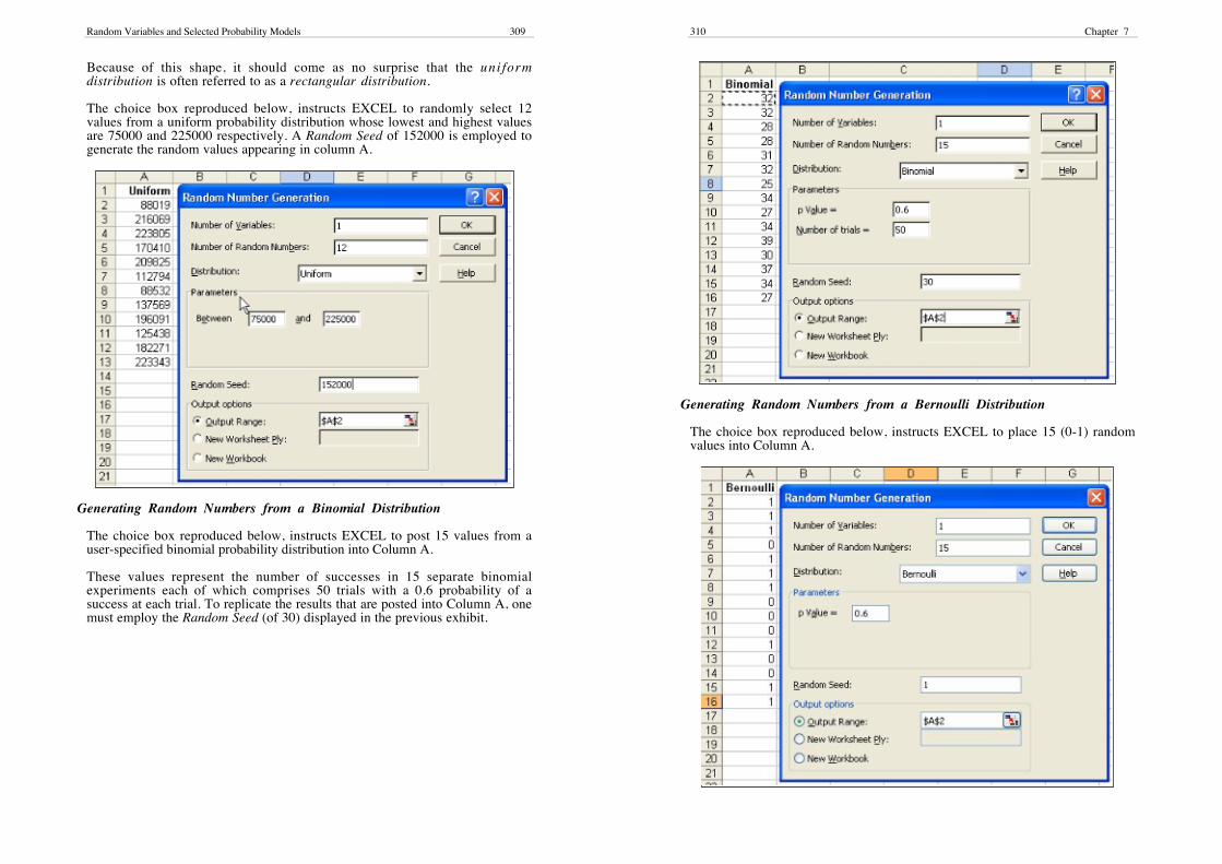
Generating Random Numbers from a Discrete Distribution
The choice box appearing below, instructs EXCEL to randomly select 12 valuesfrom a discrete probability distribution whose outcomes and associatedprobabilities are located over the cell range C2:D6. Note that the Random Seedfeature is unavailable for discrete probability distributions so that it is unlikelythat the same random values could be replicated by the reader.
Generating Random Numbers from a Uniform Distribution
A uniform distribution for a continuous random variable - not previouslydefined in this chapter - is a special distribution whose probability density isconstant over the full range of values assumed by this random variable. Thedistribution is specified by the upper and lower bounds of the range. Since, theuniform distribution has no peak, it takes the appearance of a rectangle (seeexhibit below).
lowerbound
upperbound
X (random variable)
Probability Density
Range
The Unifom or Rectangular Distribution
Random Variables and Selected Probability Models 309
Because of this shape, it should come as no surprise that the uni formdistribution is often referred to as a rectangular distribution.
The choice box reproduced below, instructs EXCEL to randomly select 12values from a uniform probability distribution whose lowest and highest valuesare 75000 and 225000 respectively. A Random Seed of 152000 is employed togenerate the random values appearing in column A.
Generating Random Numbers from a Binomial Distribution
The choice box reproduced below, instructs EXCEL to post 15 values from auser-specified binomial probability distribution into Column A.
These values represent the number of successes in 15 separate binomialexperiments each of which comprises 50 trials with a 0.6 probability of asuccess at each trial. To replicate the results that are posted into Column A, onemust employ the Random Seed (of 30) displayed in the previous exhibit.
310 Chapter 7
Generating Random Numbers from a Bernoulli Distribution
The choice box reproduced below, instructs EXCEL to place 15 (0-1) randomvalues into Column A.
Random Variables and Selected Probability Models 311
These 0-1 values indicate whether there has been a success (=1) or a failure (=0)at each of 15 separate Bernouilli experiments where the probability of a success(failure) is set to 0.60 (0.40). To replicate the results illustrated in Column A onemust employ the same Random Seed (of 1) appearing in the preceding exhibit.
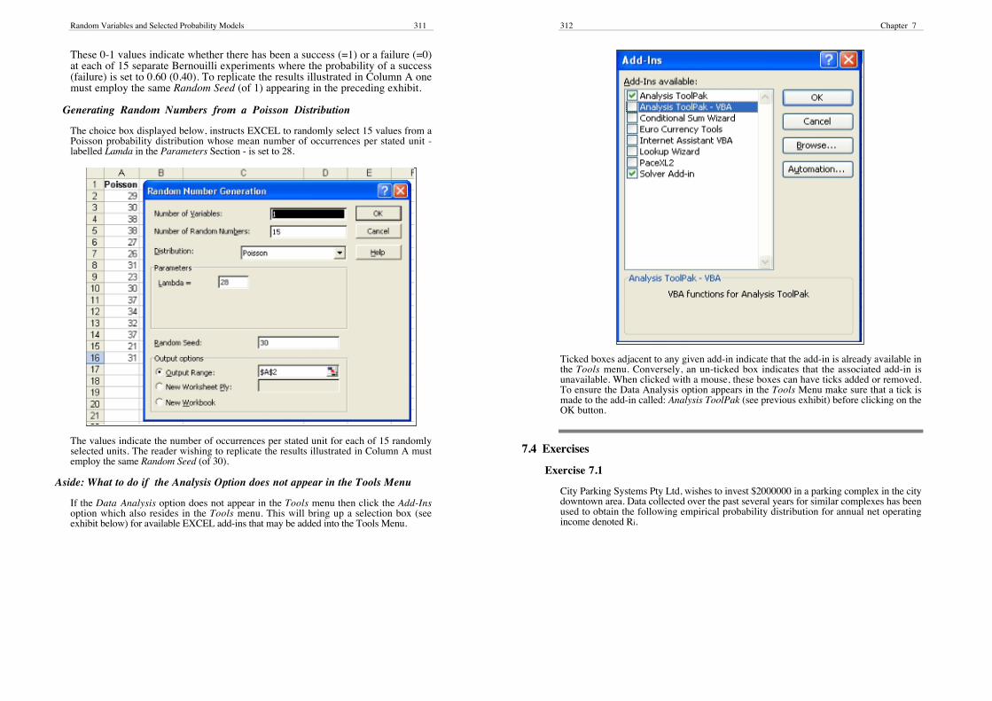
Generating Random Numbers from a Poisson Distribution
The choice box displayed below, instructs EXCEL to randomly select 15 values from aPoisson probability distribution whose mean number of occurrences per stated unit -labelled Lamda in the Parameters Section - is set to 28.
The values indicate the number of occurrences per stated unit for each of 15 randomlyselected units. The reader wishing to replicate the results illustrated in Column A mustemploy the same Random Seed (of 30).
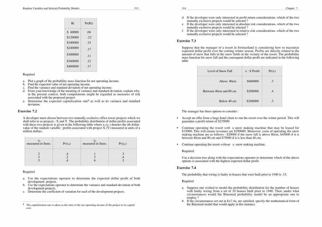
Aside: What to do if the Analysis Option does not appear in the Tools Menu
If the Data Analysis option does not appear in the Tools menu then click the Add-Insoption which also resides in the Tools menu. This will bring up a selection box (seeexhibit below) for available EXCEL add-ins that may be added into the Tools Menu.
312 Chapter 7
Ticked boxes adjacent to any given add-in indicate that the add-in is already available inthe Tools menu. Conversely, an un-ticked box indicates that the associated add-in isunavailable. When clicked with a mouse, these boxes can have ticks added or removed.To ensure the Data Analysis option appears in the Tools Menu make sure that a tick ismade to the add-in called: Analysis ToolPak (see previous exhibit) before clicking on theOK button.
7.4 Exercises
Exercise 7.1
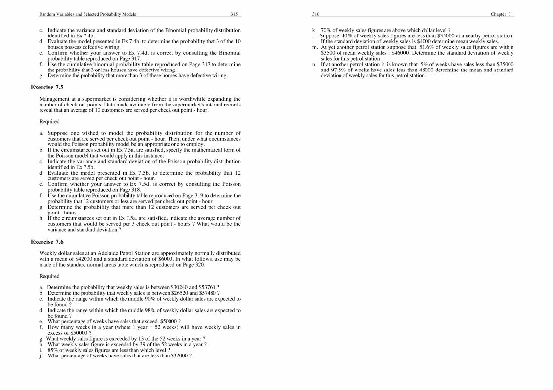
City Parking Systems Pty Ltd, wishes to invest $2000000 in a parking complex in the citydowntown area. Data collected over the past several years for similar complexes has beenused to obtain the following empirical probability distribution for annual net operatingincome denoted Ri.
Random Variables and Selected Probability Models 313
Ri Pr(Ri)
$ 60000 .06
$120000 ...22
$180000 .15
$240000 .17
$300000 .11
$360000 .12
$400000 .17
Required
a. Plot a graph of the probability mass function for net operating income.b. Find the expected value of net operating income.c. Find the variance and standard deviation of net operating income.d. From your knowledge of the meaning of variance and standard deviation, explain why,
in the present context, both computations might be regarded as measures of riskassociated with the proposed project.
e. Determine the expected capitalization rate8 as well as its variance and standarddeviation.
Exercise 7.2
A developer must choose between two mutually exclusive office tower projects which weshall refer to as projects : X and Y. The probability distribution of dollar profits associatedwith these two projects is given in the following table where xi (yi ) denotes the ith dollar-value of the random variable : profits associated with project X (Y) measured in units of amillion dollars.
ximeasured in $mio. Pr(xi)
yimeasured in $mio. Pr(yi)
2 .4 1 .33 .2 3 .45 .4 6 .3
Required
a. Use the expectations operator to determine the expected dollar profit of bothdevelopment projects.
b. Use the expectations operator to determine the variance and standard deviation of bothdevelopment projects.
c. Determine the coefficient of variation for each of the development projects.
8 The capitalization rate is taken as the ratio of the net operating income of the project to its capital cost.
314 Chapter 7
d. If the developer were only interested in profit return considerations, which of the twomutually exclusive projects would be selected ?
e. If the developer were only interested in absolute risk considerations, which of the twomutually exclusive projects would be selected ?
f. If the developer were only interested in relative risk considerations, which of the twomutually exclusive projects would be selected ?
Exercise 7.3
Suppose that the manager of a resort in Switzerland is considering how to maximizeexpected dollar profit over the coming winter season. Profits are directly related to theamount of snow that falls in the snow fields in the vicinity of the resort. The probabilitymass function for snow fall and the consequent dollar profit are indicated in the followingtable:
Level of Snow Fall x : $ Profit Pr(x)
Above 80cm $600000 .3
Between 40cm and 80 cm $200000 .4
Below 40 cm -$200000 .3
The manager has three options to consider :
• Accept an offer from a large hotel chain to run the resort over the winter period. This willguarantee a profit return of $235000
• Continue operating the resort with a snow making machine that may be leased for$15000. This will ensure revenues are $290000. Moreover, costs of operating the snowmaking machine are as follows : $20000 if the snow fall is above 80cm, $45000 if it isbetween 40cm and 80 cm and $75000 if it is less than 40 cm.
• Continue operating the resort without a snow making machine.
Required:
Use a decision tree along with the expectations operator to determine which of the aboveoptions is associated with the highest expected dollar profit.
Exercise 7.4
The probability that wiring is faulty in houses that were built prior to 1940 is .15.
Required
a. Suppose one wished to model the probability distribution for the number of houseswith faulty wiring from a set of 10 houses built prior to 1940. Then, under whatcircumstances would the Binomial probability model be an appropriate one toemploy ?
b. If the circumstances set out in Ex7.4a. are satisfied, specify the mathematical form ofthe Binomial model that would apply in this instance.
Random Variables and Selected Probability Models 315
c. Indicate the variance and standard deviation of the Binomial probability distributionidentified in Ex 7.4b.
d. Evaluate the model presented in Ex 7.4b. to determine the probability that 3 of the 10houses possess defective wiring
e. Confirm whether your answer to Ex 7.4d. is correct by consulting the Binomialprobability table reproduced on Page 317.
f. Use the cumulative binomial probability table reproduced on Page 317 to determinethe probability that 3 or less houses have defective wiring.
g. Determine the probability that more than 3 of these houses have defective wiring.
Exercise 7.5
Management at a supermarket is considering whether it is worthwhile expanding thenumber of check out points. Data made available from the supermarket's internal recordsreveal that an average of 10 customers are served per check out point - hour.
Required
a. Suppose one wished to model the probability distribution for the number ofcustomers that are served per check out point - hour. Then, under what circumstanceswould the Poisson probability model be an appropriate one to employ.
b. If the circumstances set out in Ex 7.5a. are satisfied, specify the mathematical form ofthe Poisson model that would apply in this instance.
c. Indicate the variance and standard deviation of the Poisson probability distributionidentified in Ex 7.5b.
d. Evaluate the model presented in Ex 7.5b. to determine the probability that 12customers are served per check out point - hour.
e. Confirm whether your answer to Ex 7.5d. is correct by consulting the Poissonprobability table reproduced on Page 318.
f. Use the cumulative Poisson probability table reproduced on Page 319 to determine theprobability that 12 customers or less are served per check out point - hour.
g. Determine the probability that more than 12 customers are served per check outpoint - hour.
h. If the circumstances set out in Ex 7.5a. are satisfied, indicate the average number ofcustomers that would be served per 3 check out point - hours ? What would be thevariance and standard deviation ?
Exercise 7.6
Weekly dollar sales at an Adelaide Petrol Station are approximately normally distributedwith a mean of $42000 and a standard deviation of $6000. In what follows, use may bemade of the standard normal areas table which is reproduced on Page 320.
Required
a. Determine the probability that weekly sales is between $30240 and $53760 ?b. Determine the probability that weekly sales is between $26520 and $57480 ?c. Indicate the range within which the middle 90% of weekly dollar sales are expected to
be found ?d. Indicate the range within which the middle 98% of weekly dollar sales are expected to
be found ?e. What percentage of weeks have sales that exceed $50000 ?f. How many weeks in a year (where 1 year = 52 weeks) will have weekly sales in
excess of $50000 ?g. What weekly sales figure is exceeded by 13 of the 52 weeks in a year ?h. What weekly sales figure is exceeded by 39 of the 52 weeks in a year ?i. 85% of weekly sales figures are less than which level ?j. What percentage of weeks have sales that are less than $32000 ?
316 Chapter 7
k. 70% of weekly sales figures are above which dollar level ?l. Suppose 40% of weekly sales figures are less than $35000 at a nearby petrol station.
If the standard deviation of weekly sales is $4000 determine mean weekly sales.m. At yet another petrol station suppose that 51.6% of weekly sales figures are within
$3500 of mean weekly sales : $46000. Determine the standard deviation of weeklysales for this petrol station.
n. If at another petrol station it is known that 5% of weeks have sales less than $35000and 97.5% of weeks have sales less than 48000 determine the mean and standarddeviation of weekly sales for this petrol station.
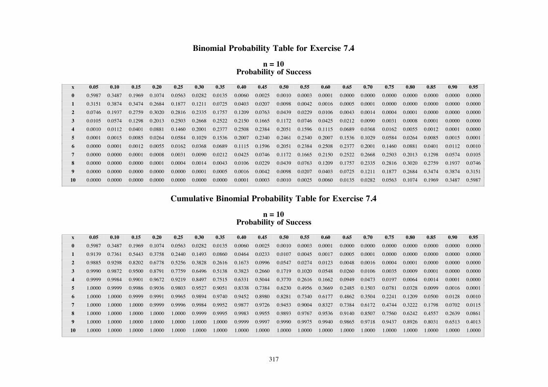
317
Binomial Probability Table for Exercise 7.4
n = 10Probability of Success
x 0.05 0.10 0.15 0.20 0.25 0.30 0.35 0.40 0.45 0.50 0.55 0.60 0.65 0.70 0.75 0.80 0.85 0.90 0.95
0 0.5987 0.3487 0.1969 0.1074 0.0563 0.0282 0.0135 0.0060 0.0025 0.0010 0.0003 0.0001 0.0000 0.0000 0.0000 0.0000 0.0000 0.0000 0.0000
1 0.3151 0.3874 0.3474 0.2684 0.1877 0.1211 0.0725 0.0403 0.0207 0.0098 0.0042 0.0016 0.0005 0.0001 0.0000 0.0000 0.0000 0.0000 0.0000
2 0.0746 0.1937 0.2759 0.3020 0.2816 0.2335 0.1757 0.1209 0.0763 0.0439 0.0229 0.0106 0.0043 0.0014 0.0004 0.0001 0.0000 0.0000 0.0000
3 0.0105 0.0574 0.1298 0.2013 0.2503 0.2668 0.2522 0.2150 0.1665 0.1172 0.0746 0.0425 0.0212 0.0090 0.0031 0.0008 0.0001 0.0000 0.0000
4 0.0010 0.0112 0.0401 0.0881 0.1460 0.2001 0.2377 0.2508 0.2384 0.2051 0.1596 0.1115 0.0689 0.0368 0.0162 0.0055 0.0012 0.0001 0.0000
5 0.0001 0.0015 0.0085 0.0264 0.0584 0.1029 0.1536 0.2007 0.2340 0.2461 0.2340 0.2007 0.1536 0.1029 0.0584 0.0264 0.0085 0.0015 0.0001
6 0.0000 0.0001 0.0012 0.0055 0.0162 0.0368 0.0689 0.1115 0.1596 0.2051 0.2384 0.2508 0.2377 0.2001 0.1460 0.0881 0.0401 0.0112 0.0010
7 0.0000 0.0000 0.0001 0.0008 0.0031 0.0090 0.0212 0.0425 0.0746 0.1172 0.1665 0.2150 0.2522 0.2668 0.2503 0.2013 0.1298 0.0574 0.0105
8 0.0000 0.0000 0.0000 0.0001 0.0004 0.0014 0.0043 0.0106 0.0229 0.0439 0.0763 0.1209 0.1757 0.2335 0.2816 0.3020 0.2759 0.1937 0.0746
9 0.0000 0.0000 0.0000 0.0000 0.0000 0.0001 0.0005 0.0016 0.0042 0.0098 0.0207 0.0403 0.0725 0.1211 0.1877 0.2684 0.3474 0.3874 0.3151
10 0.0000 0.0000 0.0000 0.0000 0.0000 0.0000 0.0000 0.0001 0.0003 0.0010 0.0025 0.0060 0.0135 0.0282 0.0563 0.1074 0.1969 0.3487 0.5987
Cumulative Binomial Probability Table for Exercise 7.4
n = 10Probability of Success
x 0.05 0.10 0.15 0.20 0.25 0.30 0.35 0.40 0.45 0.50 0.55 0.60 0.65 0.70 0.75 0.80 0.85 0.90 0.95
0 0.5987 0.3487 0.1969 0.1074 0.0563 0.0282 0.0135 0.0060 0.0025 0.0010 0.0003 0.0001 0.0000 0.0000 0.0000 0.0000 0.0000 0.0000 0.0000
1 0.9139 0.7361 0.5443 0.3758 0.2440 0.1493 0.0860 0.0464 0.0233 0.0107 0.0045 0.0017 0.0005 0.0001 0.0000 0.0000 0.0000 0.0000 0.0000
2 0.9885 0.9298 0.8202 0.6778 0.5256 0.3828 0.2616 0.1673 0.0996 0.0547 0.0274 0.0123 0.0048 0.0016 0.0004 0.0001 0.0000 0.0000 0.0000
3 0.9990 0.9872 0.9500 0.8791 0.7759 0.6496 0.5138 0.3823 0.2660 0.1719 0.1020 0.0548 0.0260 0.0106 0.0035 0.0009 0.0001 0.0000 0.0000
4 0.9999 0.9984 0.9901 0.9672 0.9219 0.8497 0.7515 0.6331 0.5044 0.3770 0.2616 0.1662 0.0949 0.0473 0.0197 0.0064 0.0014 0.0001 0.0000
5 1.0000 0.9999 0.9986 0.9936 0.9803 0.9527 0.9051 0.8338 0.7384 0.6230 0.4956 0.3669 0.2485 0.1503 0.0781 0.0328 0.0099 0.0016 0.0001
6 1.0000 1.0000 0.9999 0.9991 0.9965 0.9894 0.9740 0.9452 0.8980 0.8281 0.7340 0.6177 0.4862 0.3504 0.2241 0.1209 0.0500 0.0128 0.0010
7 1.0000 1.0000 1.0000 0.9999 0.9996 0.9984 0.9952 0.9877 0.9726 0.9453 0.9004 0.8327 0.7384 0.6172 0.4744 0.3222 0.1798 0.0702 0.0115
8 1.0000 1.0000 1.0000 1.0000 1.0000 0.9999 0.9995 0.9983 0.9955 0.9893 0.9767 0.9536 0.9140 0.8507 0.7560 0.6242 0.4557 0.2639 0.0861
9 1.0000 1.0000 1.0000 1.0000 1.0000 1.0000 1.0000 0.9999 0.9997 0.9990 0.9975 0.9940 0.9865 0.9718 0.9437 0.8926 0.8031 0.6513 0.4013
10 1.0000 1.0000 1.0000 1.0000 1.0000 1.0000 1.0000 1.0000 1.0000 1.0000 1.0000 1.0000 1.0000 1.0000 1.0000 1.0000 1.0000 1.0000 1.0000
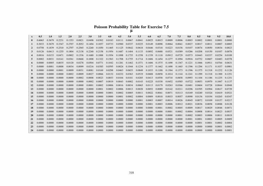
318
Poisson Probability Table for Exercise 7.5µµµµ
x 0.5 1.0 1.5 2.0 2.5 3.0 3.5 4.0 4.5 5.0 5.5 6.0 6.5 7.0 7.5 8.0 8.5 9.0 9.5 10.0
0 0.6065 0.3679 0.2231 0.1353 0.0821 0.0498 0.0302 0.0183 0.0111 0.0067 0.0041 0.0025 0.0015 0.0009 0.0006 0.0003 0.0002 0.0001 0.0001 0.0000
1 0.3033 0.3679 0.3347 0.2707 0.2052 0.1494 0.1057 0.0733 0.0500 0.0337 0.0225 0.0149 0.0098 0.0064 0.0041 0.0027 0.0017 0.0011 0.0007 0.0005
2 0.0758 0.1839 0.2510 0.2707 0.2565 0.2240 0.1850 0.1465 0.1125 0.0842 0.0618 0.0446 0.0318 0.0223 0.0156 0.0107 0.0074 0.0050 0.0034 0.0023
3 0.0126 0.0613 0.1255 0.1804 0.2138 0.2240 0.2158 0.1954 0.1687 0.1404 0.1133 0.0892 0.0688 0.0521 0.0389 0.0286 0.0208 0.0150 0.0107 0.0076
4 0.0016 0.0153 0.0471 0.0902 0.1336 0.1680 0.1888 0.1954 0.1898 0.1755 0.1558 0.1339 0.1118 0.0912 0.0729 0.0573 0.0443 0.0337 0.0254 0.0189
5 0.0002 0.0031 0.0141 0.0361 0.0668 0.1008 0.1322 0.1563 0.1708 0.1755 0.1714 0.1606 0.1454 0.1277 0.1094 0.0916 0.0752 0.0607 0.0483 0.0378
6 0.0000 0.0005 0.0035 0.0120 0.0278 0.0504 0.0771 0.1042 0.1281 0.1462 0.1571 0.1606 0.1575 0.1490 0.1367 0.1221 0.1066 0.0911 0.0764 0.0631
7 0.0000 0.0001 0.0008 0.0034 0.0099 0.0216 0.0385 0.0595 0.0824 0.1044 0.1234 0.1377 0.1462 0.1490 0.1465 0.1396 0.1294 0.1171 0.1037 0.0901
8 0.0000 0.0000 0.0001 0.0009 0.0031 0.0081 0.0169 0.0298 0.0463 0.0653 0.0849 0.1033 0.1188 0.1304 0.1373 0.1396 0.1375 0.1318 0.1232 0.1126
9 0.0000 0.0000 0.0000 0.0002 0.0009 0.0027 0.0066 0.0132 0.0232 0.0363 0.0519 0.0688 0.0858 0.1014 0.1144 0.1241 0.1299 0.1318 0.1300 0.1251
10 0.0000 0.0000 0.0000 0.0000 0.0002 0.0008 0.0023 0.0053 0.0104 0.0181 0.0285 0.0413 0.0558 0.0710 0.0858 0.0993 0.1104 0.1186 0.1235 0.1251
11 0.0000 0.0000 0.0000 0.0000 0.0000 0.0002 0.0007 0.0019 0.0043 0.0082 0.0143 0.0225 0.0330 0.0452 0.0585 0.0722 0.0853 0.0970 0.1067 0.1137
12 0.0000 0.0000 0.0000 0.0000 0.0000 0.0001 0.0002 0.0006 0.0016 0.0034 0.0065 0.0113 0.0179 0.0263 0.0366 0.0481 0.0604 0.0728 0.0844 0.0948
13 0.0000 0.0000 0.0000 0.0000 0.0000 0.0000 0.0001 0.0002 0.0006 0.0013 0.0028 0.0052 0.0089 0.0142 0.0211 0.0296 0.0395 0.0504 0.0617 0.0729
14 0.0000 0.0000 0.0000 0.0000 0.0000 0.0000 0.0000 0.0001 0.0002 0.0005 0.0011 0.0022 0.0041 0.0071 0.0113 0.0169 0.0240 0.0324 0.0419 0.0521
15 0.0000 0.0000 0.0000 0.0000 0.0000 0.0000 0.0000 0.0000 0.0001 0.0002 0.0004 0.0009 0.0018 0.0033 0.0057 0.0090 0.0136 0.0194 0.0265 0.0347
16 0.0000 0.0000 0.0000 0.0000 0.0000 0.0000 0.0000 0.0000 0.0000 0.0000 0.0001 0.0003 0.0007 0.0014 0.0026 0.0045 0.0072 0.0109 0.0157 0.0217
17 0.0000 0.0000 0.0000 0.0000 0.0000 0.0000 0.0000 0.0000 0.0000 0.0000 0.0000 0.0001 0.0003 0.0006 0.0012 0.0021 0.0036 0.0058 0.0088 0.0128
18 0.0000 0.0000 0.0000 0.0000 0.0000 0.0000 0.0000 0.0000 0.0000 0.0000 0.0000 0.0000 0.0001 0.0002 0.0005 0.0009 0.0017 0.0029 0.0046 0.0071
19 0.0000 0.0000 0.0000 0.0000 0.0000 0.0000 0.0000 0.0000 0.0000 0.0000 0.0000 0.0000 0.0000 0.0001 0.0002 0.0004 0.0008 0.0014 0.0023 0.0037
20 0.0000 0.0000 0.0000 0.0000 0.0000 0.0000 0.0000 0.0000 0.0000 0.0000 0.0000 0.0000 0.0000 0.0000 0.0001 0.0002 0.0003 0.0006 0.0011 0.0019
21 0.0000 0.0000 0.0000 0.0000 0.0000 0.0000 0.0000 0.0000 0.0000 0.0000 0.0000 0.0000 0.0000 0.0000 0.0000 0.0001 0.0001 0.0003 0.0005 0.0009
22 0.0000 0.0000 0.0000 0.0000 0.0000 0.0000 0.0000 0.0000 0.0000 0.0000 0.0000 0.0000 0.0000 0.0000 0.0000 0.0000 0.0001 0.0001 0.0002 0.0004
23 0.0000 0.0000 0.0000 0.0000 0.0000 0.0000 0.0000 0.0000 0.0000 0.0000 0.0000 0.0000 0.0000 0.0000 0.0000 0.0000 0.0000 0.0000 0.0001 0.0002
24 0.0000 0.0000 0.0000 0.0000 0.0000 0.0000 0.0000 0.0000 0.0000 0.0000 0.0000 0.0000 0.0000 0.0000 0.0000 0.0000 0.0000 0.0000 0.0000 0.0001
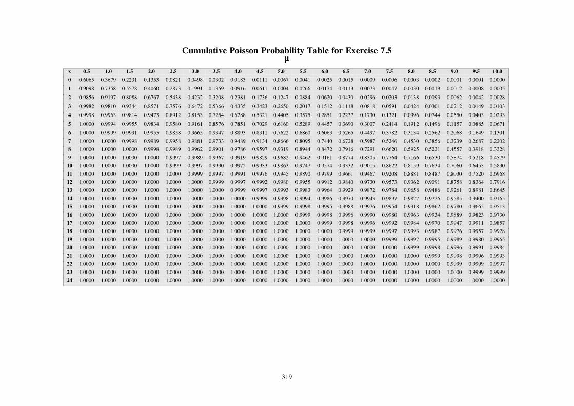
319
Cumulative Poisson Probability Table for Exercise 7.5µµµµ
x 0.5 1.0 1.5 2.0 2.5 3.0 3.5 4.0 4.5 5.0 5.5 6.0 6.5 7.0 7.5 8.0 8.5 9.0 9.5 10.0
0 0.6065 0.3679 0.2231 0.1353 0.0821 0.0498 0.0302 0.0183 0.0111 0.0067 0.0041 0.0025 0.0015 0.0009 0.0006 0.0003 0.0002 0.0001 0.0001 0.0000
1 0.9098 0.7358 0.5578 0.4060 0.2873 0.1991 0.1359 0.0916 0.0611 0.0404 0.0266 0.0174 0.0113 0.0073 0.0047 0.0030 0.0019 0.0012 0.0008 0.0005
2 0.9856 0.9197 0.8088 0.6767 0.5438 0.4232 0.3208 0.2381 0.1736 0.1247 0.0884 0.0620 0.0430 0.0296 0.0203 0.0138 0.0093 0.0062 0.0042 0.0028
3 0.9982 0.9810 0.9344 0.8571 0.7576 0.6472 0.5366 0.4335 0.3423 0.2650 0.2017 0.1512 0.1118 0.0818 0.0591 0.0424 0.0301 0.0212 0.0149 0.0103
4 0.9998 0.9963 0.9814 0.9473 0.8912 0.8153 0.7254 0.6288 0.5321 0.4405 0.3575 0.2851 0.2237 0.1730 0.1321 0.0996 0.0744 0.0550 0.0403 0.0293
5 1.0000 0.9994 0.9955 0.9834 0.9580 0.9161 0.8576 0.7851 0.7029 0.6160 0.5289 0.4457 0.3690 0.3007 0.2414 0.1912 0.1496 0.1157 0.0885 0.0671
6 1.0000 0.9999 0.9991 0.9955 0.9858 0.9665 0.9347 0.8893 0.8311 0.7622 0.6860 0.6063 0.5265 0.4497 0.3782 0.3134 0.2562 0.2068 0.1649 0.1301
7 1.0000 1.0000 0.9998 0.9989 0.9958 0.9881 0.9733 0.9489 0.9134 0.8666 0.8095 0.7440 0.6728 0.5987 0.5246 0.4530 0.3856 0.3239 0.2687 0.2202
8 1.0000 1.0000 1.0000 0.9998 0.9989 0.9962 0.9901 0.9786 0.9597 0.9319 0.8944 0.8472 0.7916 0.7291 0.6620 0.5925 0.5231 0.4557 0.3918 0.3328
9 1.0000 1.0000 1.0000 1.0000 0.9997 0.9989 0.9967 0.9919 0.9829 0.9682 0.9462 0.9161 0.8774 0.8305 0.7764 0.7166 0.6530 0.5874 0.5218 0.4579
10 1.0000 1.0000 1.0000 1.0000 0.9999 0.9997 0.9990 0.9972 0.9933 0.9863 0.9747 0.9574 0.9332 0.9015 0.8622 0.8159 0.7634 0.7060 0.6453 0.5830
11 1.0000 1.0000 1.0000 1.0000 1.0000 0.9999 0.9997 0.9991 0.9976 0.9945 0.9890 0.9799 0.9661 0.9467 0.9208 0.8881 0.8487 0.8030 0.7520 0.6968
12 1.0000 1.0000 1.0000 1.0000 1.0000 1.0000 0.9999 0.9997 0.9992 0.9980 0.9955 0.9912 0.9840 0.9730 0.9573 0.9362 0.9091 0.8758 0.8364 0.7916
13 1.0000 1.0000 1.0000 1.0000 1.0000 1.0000 1.0000 0.9999 0.9997 0.9993 0.9983 0.9964 0.9929 0.9872 0.9784 0.9658 0.9486 0.9261 0.8981 0.8645
14 1.0000 1.0000 1.0000 1.0000 1.0000 1.0000 1.0000 1.0000 0.9999 0.9998 0.9994 0.9986 0.9970 0.9943 0.9897 0.9827 0.9726 0.9585 0.9400 0.9165
15 1.0000 1.0000 1.0000 1.0000 1.0000 1.0000 1.0000 1.0000 1.0000 0.9999 0.9998 0.9995 0.9988 0.9976 0.9954 0.9918 0.9862 0.9780 0.9665 0.9513
16 1.0000 1.0000 1.0000 1.0000 1.0000 1.0000 1.0000 1.0000 1.0000 1.0000 0.9999 0.9998 0.9996 0.9990 0.9980 0.9963 0.9934 0.9889 0.9823 0.9730
17 1.0000 1.0000 1.0000 1.0000 1.0000 1.0000 1.0000 1.0000 1.0000 1.0000 1.0000 0.9999 0.9998 0.9996 0.9992 0.9984 0.9970 0.9947 0.9911 0.9857
18 1.0000 1.0000 1.0000 1.0000 1.0000 1.0000 1.0000 1.0000 1.0000 1.0000 1.0000 1.0000 0.9999 0.9999 0.9997 0.9993 0.9987 0.9976 0.9957 0.9928
19 1.0000 1.0000 1.0000 1.0000 1.0000 1.0000 1.0000 1.0000 1.0000 1.0000 1.0000 1.0000 1.0000 1.0000 0.9999 0.9997 0.9995 0.9989 0.9980 0.9965
20 1.0000 1.0000 1.0000 1.0000 1.0000 1.0000 1.0000 1.0000 1.0000 1.0000 1.0000 1.0000 1.0000 1.0000 1.0000 0.9999 0.9998 0.9996 0.9991 0.9984
21 1.0000 1.0000 1.0000 1.0000 1.0000 1.0000 1.0000 1.0000 1.0000 1.0000 1.0000 1.0000 1.0000 1.0000 1.0000 1.0000 0.9999 0.9998 0.9996 0.9993
22 1.0000 1.0000 1.0000 1.0000 1.0000 1.0000 1.0000 1.0000 1.0000 1.0000 1.0000 1.0000 1.0000 1.0000 1.0000 1.0000 1.0000 0.9999 0.9999 0.9997
23 1.0000 1.0000 1.0000 1.0000 1.0000 1.0000 1.0000 1.0000 1.0000 1.0000 1.0000 1.0000 1.0000 1.0000 1.0000 1.0000 1.0000 1.0000 0.9999 0.9999
24 1.0000 1.0000 1.0000 1.0000 1.0000 1.0000 1.0000 1.0000 1.0000 1.0000 1.0000 1.0000 1.0000 1.0000 1.0000 1.0000 1.0000 1.0000 1.0000 1.0000
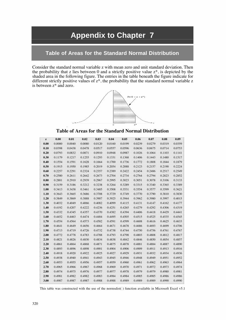
320
Appendix to Chapter 7
Table of Areas for the Standard Normal Distribution
Consider the standard normal variable z with mean zero and unit standard deviation. Thenthe probability that z lies between 0 and a strictly positive value z*, is depicted by theshaded area in the following figure. The entries in the table beneath the figure indicate fordifferent strictly positive values of z*, the probability that the standard normal variable zis between z* and zero.
Table of Areas for the Standard Normal Distribution
z 0.00 0.01 0.02 0.03 0.04 0.05 0.06 0.07 0.08 0.09
0.00 0.0000 0.0040 0.0080 0.0120 0.0160 0.0199 0.0239 0.0279 0.0319 0.0359
0.10 0.0398 0.0438 0.0478 0.0517 0.0557 0.0596 0.0636 0.0675 0.0714 0.0753
0.20 0.0793 0.0832 0.0871 0.0910 0.0948 0.0987 0.1026 0.1064 0.1103 0.1141
0.30 0.1179 0.1217 0.1255 0.1293 0.1331 0.1368 0.1406 0.1443 0.1480 0.1517
0.40 0.1554 0.1591 0.1628 0.1664 0.1700 0.1736 0.1772 0.1808 0.1844 0.1879
0.50 0.1915 0.1950 0.1985 0.2019 0.2054 0.2088 0.2123 0.2157 0.2190 0.2224
0.60 0.2257 0.2291 0.2324 0.2357 0.2389 0.2422 0.2454 0.2486 0.2517 0.2549
0.70 0.2580 0.2611 0.2642 0.2673 0.2704 0.2734 0.2764 0.2794 0.2823 0.2852
0.80 0.2881 0.2910 0.2939 0.2967 0.2995 0.3023 0.3051 0.3078 0.3106 0.3133
0.90 0.3159 0.3186 0.3212 0.3238 0.3264 0.3289 0.3315 0.3340 0.3365 0.3389
1.00 0.3413 0.3438 0.3461 0.3485 0.3508 0.3531 0.3554 0.3577 0.3599 0.3621
1.10 0.3643 0.3665 0.3686 0.3708 0.3729 0.3749 0.3770 0.3790 0.3810 0.3830
1.20 0.3849 0.3869 0.3888 0.3907 0.3925 0.3944 0.3962 0.3980 0.3997 0.4015
1.30 0.4032 0.4049 0.4066 0.4082 0.4099 0.4115 0.4131 0.4147 0.4162 0.4177
1.40 0.4192 0.4207 0.4222 0.4236 0.4251 0.4265 0.4279 0.4292 0.4306 0.4319
1.50 0.4332 0.4345 0.4357 0.4370 0.4382 0.4394 0.4406 0.4418 0.4429 0.4441
1.60 0.4452 0.4463 0.4474 0.4484 0.4495 0.4505 0.4515 0.4525 0.4535 0.4545
1.70 0.4554 0.4564 0.4573 0.4582 0.4591 0.4599 0.4608 0.4616 0.4625 0.4633
1.80 0.4641 0.4649 0.4656 0.4664 0.4671 0.4678 0.4686 0.4693 0.4699 0.4706
1.90 0.4713 0.4719 0.4726 0.4732 0.4738 0.4744 0.4750 0.4756 0.4761 0.4767
2.00 0.4772 0.4778 0.4783 0.4788 0.4793 0.4798 0.4803 0.4808 0.4812 0.4817
2.10 0.4821 0.4826 0.4830 0.4834 0.4838 0.4842 0.4846 0.4850 0.4854 0.4857
2.20 0.4861 0.4864 0.4868 0.4871 0.4875 0.4878 0.4881 0.4884 0.4887 0.4890
2.30 0.4893 0.4896 0.4898 0.4901 0.4904 0.4906 0.4909 0.4911 0.4913 0.4916
2.40 0.4918 0.4920 0.4922 0.4925 0.4927 0.4929 0.4931 0.4932 0.4934 0.4936
2.50 0.4938 0.4940 0.4941 0.4943 0.4945 0.4946 0.4948 0.4949 0.4951 0.4952
2.60 0.4953 0.4955 0.4956 0.4957 0.4959 0.4960 0.4961 0.4962 0.4963 0.4964
2.70 0.4965 0.4966 0.4967 0.4968 0.4969 0.4970 0.4971 0.4972 0.4973 0.4974
2.80 0.4974 0.4975 0.4976 0.4977 0.4977 0.4978 0.4979 0.4979 0.4980 0.4981
2.90 0.4981 0.4982 0.4982 0.4983 0.4984 0.4984 0.4985 0.4985 0.4986 0.4986
3.00 0.4987 0.4987 0.4987 0.4988 0.4988 0.4989 0.4989 0.4989 0.4990 0.4990
This table was constructed with the use of the normsdist( ) function available in Microsoft Excel v5.1