Copyright © 2005 Brooks/Cole, a division of Thomson Learning, Inc. 7.1 Random Variables and Discrete Probability Distributions

Copyright © 2005 Brooks/Cole, a division of Thomson Learning, Inc. 7.1

Random Variables andDiscrete Probability

Distributions


Random Variables…

A random variable is a function or rule that assigns a number to each outcome of an experiment. Basically it is just a symbol that represents the outcome of an experiment.

X = number of heads when the experiment is flipping a coin 20 times.

C = the daily change in a stock price.

R = the number of miles per gallon you get on your auto during a family vacation.

Y = the amount of medication in a blood pressure pill.

V = the speed of an auto registered on a radar detector used on I-20


Two Types of Random Variables… Discrete Random Variable – usually count data [Number of]

* one that takes on a countable number of values – this means you can sit down and list all possible outcomes without missing any, although it might take you an infinite amount of time.X = values on the roll of two dice: X has to be either 2, 3, 4, …, or 12.Y = number of accidents on the UTA campus during a week: Y has to be 0, 1, 2, 3, 4, 5, 6, 7, 8, ……………”real big number”

Continuous Random Variable – usually measurement data [time, weight, distance, etc]

* one that takes on an uncountable number of values – this means you can never list all possible outcomes even if you had an infinite amount of time.X = time it takes you to drive home from class: X > 0, might be 30.1 minutes measured to the nearest tenth but in reality the actual time is 30.10000001…………………. minutes?)

Exercise: try to list all possible numbers between 0 and 1.


Probability Distributions…

A probability distribution (density function) is a table, formula, or graph that describes the values of a random variable and the probability associated with these values.

– Discrete Probability Distribution

X = outcome of rolling one die

– Continuous Probability Distribution

X 1 2 3 4 5 6P(X) 1/6 1/6 1/6 1/6 1/6 1/6


Discrete Probability Notation…

An upper-case letter will represent the name of the random variable, usually X.

Its lower-case counterpart, x, will represent the value of the random variable.

The probability that the random variable X will equal x is:

P(X = x) or more simply P(x)

X = number of heads in 10 flips of coin

P(X = 5) = P(5) = probability of 5 heads (x) in 10 flips


Discrete Probability Distributions…

Probabilities, P(x), associated with Discrete random variables have the following properties.

X 1 2 3 4 5 6P(X) 1/6 1/6 1/6 1/6 1/6 1/6


Developing Discrete Probability DistributionsProbability distributions can be estimated from relative frequencies. Consider the discrete (countable) number of televisions per household (X) from US survey data (Example 7.1)…

1,218 ÷ 101,501 = 0.012

e.g. P(X=4) = P(4) = 0.076 = 7.6%


Questions you might want answered

E.g. what is the probability there is at least one television but no more than three in any given household?

“at least one television but no more than three”P(1 ≤ X ≤ 3) = P(1) + P(2) + P(3) = .319 + .374 + .191 = .884

Copyright © 2005 Brooks/Cole, a division of Thomson Learning, Inc.

In most college courses, you get as a grade, either an A, B, C, D, or F. For credit purposes, A’s aregiven 4 points, B’s are given 3 points, C’s are given 2 points, Ds are given 1 point, and F’s are no points.

Let X be the random variable representing the points a student gets. What are the possible values of X?

7.9

The possible values of X are 4, 3, 2, 1, and 0.

Example


Example

Value of X

P(X)

7.10

A college instructor teaching a large class traditionally gives 10% A’s, 20% B’s, 45% C’s, 15% D’s, and 10% F’s. If a student is chosen at random from the class, the student’s grade on a 4-point scale (A = 4) is a random variable X. Create the distribution of X.

What is the probability that a student has a grade point of 3 or better in this class?

What is the probability that a student has a grade point of 2 or worse in this class?

Draw a probability histogram to picture the probability distribution of the random variable X.


Discrete Probability Distribution

The mean of a discrete random variable is the weighted average of all of its values. The weights are the probabilities. This parameter is also called the expected value of X and is represented by E(X).

The variance is

The standard deviation is


Example

Value of X 0 1 2 3 4

P(X) .10 .15 .45 .20 .10

7.12

A college instructor teaching a large class traditionally gives 10% A’s, 20% B’s, 45% C’s, 15% D’s, and 10% F’s. If a student is chosen at random from the class, the student’s grade on a 4-point scale (A = 4) is a random variable X. Create the distribution of X.

Find the mean (expected value) and standard deviation for the probability distribution.


Example

A fair coin is flipped 3 times. Find the mean and standard deviation of the discrete random variable X that counts the number of heads.

7.13


Example

The daily lottery costs $1 to play. You pick a 3 digit number. If you win, you win $500. Find the expected value and standard deviation of the lottery.

7.14


Example

Choose an American household at random and let the random variable X be the number of persons living in the household. Find the mean and standard deviation of the average American household.

7.15


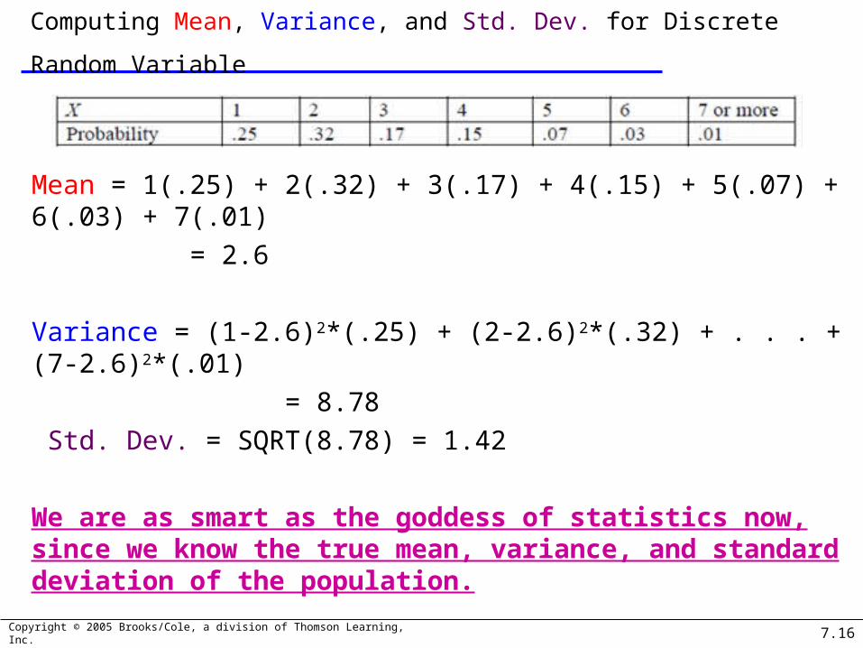
Computing Mean, Variance, and Std. Dev. for Discrete Random

Variable

Mean = 1(.25) + 2(.32) + 3(.17) + 4(.15) + 5(.07) + 6(.03) + 7(.01)

= 2.6

Variance = (1-2.6)2*(.25) + (2-2.6)2*(.32) + . . . + (7-2.6)2*(.01)

= 8.78

Std. Dev. = SQRT(8.78) = 1.42

We are as smart as the goddess of statistics now, since we know the true mean, variance, and standard deviation of the population.


Rules for means

7.17

Example: You play two casino games. Game 1 has an expectation of losing $1 a play and game 2 has an expectation of losing $2 a play. If you play both games, what is your expectation for both games.

Example: You go to a casino and play the same slot machine which averages losing 15 cents a play. You play the machine 100 times and then leave, paying $5 for parking. Find your expectation for your casino visit.


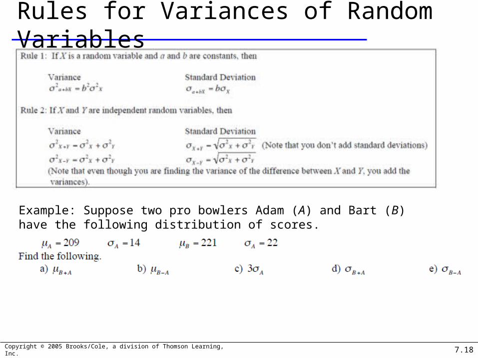
Rules for Variances of Random Variables

7.18

Example: Suppose two pro bowlers Adam (A) and Bart (B) have the following distribution of scores.


ExampleDepending on the attendance of a minor league baseball team,

the number of hot dogs and sodas sold at a game is given by the following table.

Find the standard deviation of the number of hot dogs plus the number of sodas sold.

7.19


Example: You weight all 30,000 studentsRandom Variable: X = students weightMean(X) = X-Bar = 160 lbsVariance(X) = s2 = 900 lbs2

StdDev(X) = s = 30 lbs*************************************You now discover that the scales reported a student’s weight 5 lbs too heavy. The student’s real weights (Y) should have been Y = X – 5. What are the mean and variance of the student’s REAL weightsMean(Y) = Mean(X) – 5 = 160 – 5 = 155 lbsVariance(Y) = Variance(X) = 900StdDev(Y) = SQRT(900) = 30


Example: You measure the height of all 30,000 students

Random Variable: X = students height in “Feet”

Mean(X) = X-Bar = 5.8 feet

Variance(X) = s2 = 0.09 feet2

StdDev(X) = s = 0.3 feet

*************************************

You now discover that the President wanted to measure student’s heights in “Inches” and not “Feet”. The student’s height in “Inches” (Y) should have been Y = 12*X . What are the mean and variance of the student’s heights in Inches?

Mean(Y) = 12*Mean(X) = 12*5.8 = 69.6 inches

Variance(Y) = 122*Variance(X) = 144*(.09) = 12.96

StdDev(Y) = SQRT(12.96) = 3.6


Laws…We can derive laws of expected value and variance for the sum of two independent

random variables as follows…E(X + Y) = E(X) + E(Y)V(X + Y) = V(X) + V(Y) **************************************************************X = weight of right shoes: Mean(X) = .5 lbs and Var(X) = .0004Y = weight of left shoes: Mean(Y) = .5 lbs and Var(Y) = .0004**************************************************************What is the mean and variance of a “Pair” of shoes. P = X +YE(P) = E(X + Y) = E(X) + E(Y) = .5 + .5 = 1.0V(P) = V(X+Y) = V(X) + V(Y) = .0004 + .0004 = .0008

NOTE: WEIGHTS OF RIGHT AND LEFT SHOE INDEPENDENT***************************************************************

? How could you determine the mean and variance of the weight of an automobile after you make all the parts but before you assemble the automobile


Binomial Distribution… 2 parameters [n and p]The binomial distribution is the probability distribution that

results from doing a “binomial experiment”. Binomial experiments have the following properties:

1. Fixed number of trials, represented as n.

2. Each trial has two possible outcomes, a “success” and a “failure”.

3. P(success)=p (and thus: P(failure)=1–p), for all trials.

4. The trials are independent, which means that the outcome of one trial does not affect the outcomes of any other trials.


Success and Failure……are just labels for a binomial experiment, there is no value judgment implied. You may define either one of the 2 possible outcomes as “Success”

For example a coin flip will result in either heads or tails. If we define “heads” as success then necessarily “tails” is considered a failure (inasmuch as we attempting to have the coin lands heads up).

Other potential examples of binomial random variables:– A firecracker pops or fails to pop– A patient get an infection during an operation or does not get an infection


Binomial Random Variable…The random variable of a binomial experiment is defined as the number of successes, X, in the n trials, where the probability of success on a single trial is p.

E.g. flip a fair coin 10 times…

1) Fixed number of trials n=10

2) Each trial has two possible outcomes {heads (success), tails (failure)}

3) P(success)= 0.50; P(failure)=1–0.50 = 0.50 4) The trials are independent (i.e. the outcome of heads on the first flip will have no impact on subsequent coin flips).

Hence flipping a coin ten times is a binomial experiment since all conditions were met.


Are these examples of binomial distributions?1) Tossing 20 coins and counting the number of heads.

1) Success is a heads, failure is a tails. 2) n = 20 3) Independence is true – coins have no influence on each other 4) p = .5.

So X is B(20, .5). The possible values of X are the integers from 0 to 20.

2) Picking 5 cards from a standard deck and counting the number of hearts. We replace the card each time and reshuffle.1) Success is a heart, failure is anything but a heart. 2) n = 5. 3) Independence is true. 4) p =.25.


7.26


Are these examples of binomial distributions?3) Picking 5 cards from a standard deck and counting the number of hearts

without reshuffling.This is not binomial because of the independence issue.

4) Choosing a card from a standard deck until you get a heart.This is not binomial as there are not a fixed number of observations.

5) It is estimated that 87% of computers users use Explorer as their default web browser. We choose 50 computer users and ask their default browser.1) Success is Explorer, failure is anything else.2) n =50. 3) Independence seems logical.4) p = .87.


7.27


Binomial Distribution [formula]

The binomial random variable (# of successes in n trials) take on values 0, 1, 2, …, n. Thus, its a discrete random variable.

Once we know a random variable is binomial, we can calculate the probability associated with each value of the random variable from the binomial distribution:

where n = number in sample p = probability of success

k = # successes and n-k = # failures

!

! !n k

nC

k n k


Problem: Pat Statsdud…

Pat Statsdud failed to study for the next stat exam. Pat’s exam strategy is to rely on luck for the next quiz. The quiz consists of 10 multiple-choice questions (n=10). Each question has five possible answers, only one of which is correct (p=0.2). Pat plans to guess the answer to each question.

What is the probability that Pat gets no answers correct?

P(X=0) = P(0) =

What is the probability that Pat gets two answers correct?

P(X=2) = P(2) =


Pat Statsdud…

n=10, and P(success) = .20

What is the probability that Pat gets no answers correct?

I.e. # success, x, = 0; hence we want to know P(x=0)

Pat has about an 11% chance of getting no answers correctusing the guessing strategy.


Pat Statsdud…

n=10, and P(success) = .20

What is the probability that Pat gets two answers correct?

I.e. # success, x, = 2; hence we want to know P(x=2)

Pat has about a 30% chance of getting exactly two answerscorrect using the guessing strategy.


Example

You toss 5 coins. What is the probability that you get 3 heads?

7.32

( ) (1 )k n knP X k p p

k


Cumulative Probability…“Find the probability that Pat fails the quiz”

If a grade on the quiz is less than 50% (i.e. 5 questions

out of 10), that’s considered a failed quiz.

P(fail quiz) = P(X < 4) = P(0)+P(1)+P(2)+P(3)+P(4)

Called a cumulative probability, that is, P(X ≤ x)

Note: Calculating all these individual probabilities would be tedious and time consuming, however, the Binomial tables at back of book gives you the cumulative probabilities [n=10, p=0.2, x=4]


Pat Statsdud…Calculate Individual Probabilities and Add Up!P(X ≤ 4) = P(0) + P(1) + P(2) + P(3) + P(4)

We already know P(0) = .1074 and P(2) = .3020. Using the binomial formula to calculate the others:P(1) = .2684 , P(3) = .2013, and P(4) = .0881

Hense P(X ≤ 4) = .1074 + .2684 + … + .0881 = .9672

ORUse binomial tables at back of book for n=10, p=0.2, and x=4 OR Use CALCULATOR!


Calculator

binompdf(number of trials, probability of success, number of success)

Used to compute binomial probabilities for a particular number of successes.

binomcdf(number of trials, probability, number of successes or less)

Used to compute cumulative (from smaller) successes.

7.35


ExampleWill Guess takes a true-false test of 6 questions and has

absolutely no idea of any of the answers.So, true to his name, he guesses on all of them. If 4 questions

correct is passing, what is the probability that he passes the exam?

7.36

Suppose the test above is now multiple choice with 4 answers per problem and again, Will Guesses.Find the probability that he passes the test and the expected number of passing students in a school of 1,500 ifthey all guessed.


Example

In a particular city, 63% of the adults own their home and 37% rent. A sample of 20 adults is taken.

Find the probability that the sample will have at least half home-owners.

7.37


Binomial Distribution…As you might expect, statisticians have determined formulas for the mean, variance, and standard deviation of a binomial random variable. They are:

Previous example: n=10, p=0.2μ = n*p = 10*0.2 = 2σ2 = n*p*(1-p) = 10*0.2*0.8= 1.6σ = SQRT(1.6) = 1.26


Example

A basketball player is traditionally a 72% foul shooter. In a season, he takes 427 foul shots. Find

the mean and standard deviation of the distribution.

7.39


Geometric Random Variables Only two possible outcomes (success or failure)

Probability of success is constant for each trial

Each trial is independent of other trials

Looking for the number of trials to obtain the FIRST success

7.40


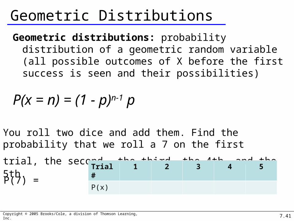
Geometric DistributionsGeometric distributions: probability distribution of a

geometric random variable (all possible outcomes of X before the first success is seen and their possibilities)

P(x = n) = (1 - p)n-1 p

7.41

You roll two dice and add them. Find the probability that we roll

a 7 on the first trial, the second, the third, the 4th, and the 5th.

P(7) =

Trial # 1 2 3 4 5

P(x)


Calculator

geometpdf(probability of success, number of trials)

Use for computing geom. probabilities for a particular number of trials.

geometcdf (probability of success, number of trials)

Use for computing geom. probabilities of a given number of trials or less (cumulative from smaller end)

7.42


Example

It is estimated that 45% of people in Fast-Food restaurants order a diet drink with their lunch.

Find the probability that the fourth person orders a diet drink.

Also find the probability that the first dietdrinker of the day occurs before the 5th person.

7.43


Mean and Standard deviational

7.44

1X p

2

1X

p

p

Standard deviation of geometric random variable X:

Mean of geometric random variable X:

In New York City at rush hour, the chance that a taxicab passes someone and is available is 15%.a)How many cabs can you expect to pass you for you to find one that is free? b) What is the probability that more than 10 cabs pass you before you find one that is free?



Poisson Distribution… 1 parameter [μ]Named for Simeon Poisson, the Poisson distribution is a discrete probability distribution and refers to the number of events (a.k.a. successes) within a specific time period or region of space. For example:

• The number of cars arriving at a service station in 1 hour. (The interval of time is 1 hour.)

• The number of flaws in a bolt of cloth. (The specific region is a bolt of cloth.)

• The number of accidents in 1 day on a particular stretch of highway. (The interval is defined by both time, 1 day, and space, the particular stretch of highway.)


Poisson Probability Distribution…

The probability that a Poisson random variable assumes a value of x is given by:

Note: μ is the only parameter [tell me μ and I can calculate the probabilities]and e is the natural logarithm base.

FYI:


Example 7.12…

The number of typographical errors in new editions of textbooks varies considerably from book to book. After some analysis he concludes that the number of errors is Poisson distributed with a mean of 1.5 typos per 100 pages. The instructor randomly selects 100 pages of a new book. What is the probability that there are no typos?

That is, what is P(X=0) given that = 1.5?

“There is about a 22% chance of finding zero errors”


Poisson Distribution…

As mentioned on the Poisson experiment slide:

The probability of a success is proportional to the size of the interval

Thus, knowing an error rate of 1.5 typos per 100 pages, we can determine a mean value for a 400 page book as:

=1.5(4) = 6 typos / 400 pages.


Example 7.13…

For a 400 page book, what is the probability that there are

no typos?

P(X=0) =

“there is a very small chance there are no typos”


Example 7.13…

For a 400 page book, what is the probability that there are five or less typos?

P(X≤5) = P(0) + P(1) + … + P(5)

This is rather tedious to solve manually. A better alternative is to refer to Table 2 in Appendix B…

…k=5, =6, and P(X ≤ k) = .446

“there is about a 45% chance there are 5 or less typos”


Example 7.13…

…Excel is an even better alternative:


Poisson Practice

The number of infections [X] in a hospital each week has been shown to follow a poisson distribution with mean 3.0 infections per week. Calculate the following probabilities.•P(X = 0) =

•P(X < 4) =

•P(X > 9) =

•If you found 9 infections next week, what would you say??

Documents

Copyright © 2005 Brooks/Cole, a division of Thomson Learning, Inc. 7.1 Random Variables and Discrete Probability Distributions