Fightin’ Words: Lexical Feature Selection and Evaluation for Identifying …languagelog.ldc.upenn.edu/myl/Monroe.pdf · Fightin’ Words: Lexical Feature Selection and ... Our proposed

Advance Access publication February 16, 2009 Political Analysis (2008) 16:372–403doi:10.1093/pan/mpn018

Fightin’ Words: Lexical Feature Selection andEvaluation for Identifying the Content of Political

Conflict

Burt L. Monroe

Department of Political Science, Quantitative Social Science Initiative, The Pennsylvania

State University, e-mail: [email protected] (corresponding author)

Michael P. Colaresi

Department of Political Science, Michigan State University, e-mail: [email protected]

Kevin M. Quinn

Department of Government and Institute for Quantitative Social Science, Harvard University,

e-mail: [email protected]

Entries in the burgeoning ‘‘text-as-data’’ movement are often accompanied by lists or

visualizations of how word (or other lexical feature) usage differs across some pair or set of

documents. These are intended either to establish some target semantic concept (like the

content of partisan frames) to estimate word-specific measures that feed forward into

another analysis (like locating parties in ideological space) or both. We discuss a variety of

techniques for selecting words that capture partisan, or other, differences in political speech

and for evaluating the relative importance of those words. We introduce and emphasize

several new approaches based on Bayesian shrinkage and regularization. We illustrate the

relative utility of these approaches with analyses of partisan, gender, and distributive speech

in the U.S. Senate.

1 Introduction

As new approaches to, and applications of, the ‘‘text-as-data’’ movement emerge, we findourselves presented with many collections of disembodied words. Newspaper articles,blogs, and academic papers burst with lists of words that vary or discriminate across groupsof documents (Gentzkow and Shapiro 2006; Quinn et al. 2006; Diermeier et al. 2007;Sacerdote and Zidar 2008; Yu et al. 2008), pictures of words scaled in some political space(Schonhardt-Bailey 2008), or both (Monroe and Maeda 2004; Slapin and Proksch 2008).These word or feature lists and graphics are one of the most intuitive ways to convey the

Author’s note: We would like to thank Mike Crespin, Jim Dillard, Jeff Lewis, Will Lowe, Mike MacKuen, AndrewMartin, Prasenjit Mitra, Phil Schrodt, Corwin Smidt, Denise Solomon, Jim Stimson, Anton Westveld, Chris Zorn,and participants in seminars at the University of North Carolina, Washington University, and Pennsylvania StateUniversity for helpful comments on earlier and related efforts. Any opinions, findings, and conclusions or rec-ommendations expressed in the paper are those of the authors and do not necessarily reflect the views of theNational Science Foundation.

� The Author 2009. Published by Oxford University Press on behalf of the Society for Political Methodology.All rights reserved. For Permissions, please email: [email protected]

372

at University of Pennsylvania L

ibrary on June 3, 2013http://pan.oxfordjournals.org/

Dow

nloaded from

http://pan.oxfordjournals.org/

key insight from such analyses—the content of a politically interesting difference. Accord-ingly, we notice when such analyses 1) produce key word lists with odd conceptualmatches,1 2) remove words from lists before presenting them to the reader (Diermeieret al. 2007) or 3) produce no word lists or pictures at all (Hillard et al. 2007; Hopkinsand King 2007).

These word visualizations and lists are common because they serve three importantroles. First, they are often intended (implicitly) to offer semantic validity to an automatedcontent analysis—to ensure that substantive meaning is being captured by some text-as-data measure (Krippendorff 2004). That is, the visualizations reflect either a selection ofwords or a word-specific measure that is intended to characterize some semantic politicalconcept of direct interest, for example, topic (Quinn et al. 2006), ideology (Diermeier et al.2007), or competitive frame (Schonhardt-Bailey 2008). Second, the visualizations reflecteither a selection of words or a word-specific measure that is intended to feed forward tosome other analysis. For example, these word estimates might be used to train a classifierfor uncoded documents (Yu et al. 2008), to scale future party manifestos against past ones(Laver et al. 2003), to scale individual legislators relative to their parties (Monroe andMaeda 2004), or to evaluate partisan bias in media sources (Gentzkow and Shapiro2006). Third and more broadly, the political content of the words themselves—words tellus what they mean—allows word lists and visualizations of words to compactly present thevery political content and cleavages that justify the enterprise. If we cannot find principledways to meaningfully sort, organize, and summarize the substantial and at times over-whelming information captured in speech, the promise of using speeches and words asobservations to be statistically analyzed is severely compromised.

In this paper, we take a closer look at methods for identifying and weighting words andfeatures that are used distinctly by one or more political groups or actors. We demonstratesome fundamental problems with common methods used for this purpose. Major problemsinclude failure to account for sampling variation and overfitting of idiosyncratic differen-ces. Having diagnosed these problems, we offer two new approaches to the problem ofidentifying political content. Our proposed solution relies on a model-based approachto avoid inefficiency and shrinkage and regularization to avoid both infinite estimatesand overfitting the sample data. We illustrate the usefulness of these methods by examiningpartisan framing, the content of representation and polarization over time, and the dimen-sionality of politics in the U.S. Senate.

2 The Objectives: Feature Selection and Evaluation

There are two slightly different goals to be considered here: feature selection and featureevaluation. With feature selection, the primary goal is a binary decision—in or out—for theinclusion of features in some subsequent analysis. We might, for example, want to knowwhich words are reliably used differently by two political parties. This might be for thepurpose of using these features in a subsequent model of individual speaker positioning orfor a qualitative evaluation of the ideological content of party competition to give twoexamples. In the former case, fear of overfitting leads us to prefer parsimonious specifi-cations, as with variable selection in regression. In the latter case, computers can estimate but

1Motorway is a Labour word? (Laver et al. 2003). The single most Republican word is meth? (Yu et al. 2008). Theword that best defines the ideological left in Germany is pornographie? (Slapin and Proksch 2008). Martin LutherKing and Ronald Reagan’s speeches were distinguished by the use of him (MLK) and she (Reagan)? (Sacerdoteand Zidar 2008).

373Fightin’ Words



Dow

nloaded from


not interpretourmodels;data reduction isnecessary to reduce thequantityof information thatmust be processed by the analyst. Further, the scale of speech data is immense. Feature se-lection is useful because we necessarily need a lower dimensional summary of the sampledata.Additionally,weknowapriori thatdifferentspeechpatternsacrossgroupscanflowfromboth partisan and nonpartisan sources, including idiosyncrasies of dialect and style.

With feature evaluation, the goal is to quantify our information about different features.We want to know, for example, the extent to which each word is used differently by twopolitical parties. This might be used to tell us how to weight features in a subsequent modelor allow us, in the qualitative case, to have some impression of the relative importanceof each word for defining the content of the partisan conflict. The question is not whichof these terms are partisan and which are not, but which are the most partisan, on whichside, and by how much. Again, in all these cases, parsimony and clarity are virtues. Over-fitting should be guarded against because 1) we are interested, not solely in the sample data,but inferring externally valid regularities from that sample data and 2) a list of thousandsof words, all of which are approximately equal in weight, is less useful than a list thatis winnowed and summarized by some useful criterion.

3 Methods for Lexical Feature Selection and Evaluation

To fix ideas, we use a running example, identifying and evaluating the linguistic differencesbetween Democrats and Republicans in U.S. Senate speeches on a given topic. The topicswe use, like ‘‘Defense’’ or ‘‘Judicial Nominations’’ or ‘‘Taxes’’ or ‘‘Abortion’’, are thosethat emerge from the topic model of Senate speech from 1997 to 2004 discussed in Quinnet al. (2006).2 In this section, our running example is an analysis of speeches deliveredon the topic of ‘‘Abortion’’ during the 106th Congress (1999–2000), often the subjectof frame analysis (Adams 1997; McCaffrey and Keys 2008; Schonhardt-Bailey 2008).3

The familiarity of this context makes clear the presence, or absence, of semantic validityunder different methods.

Thelessonsareeasilygeneralizedandapplied toothercontexts (gender,electoraldistricts,opposition status, multiparty systems, etc.), which we demonstrate in the final section. Wetake the set of potentially relevant lexical features to be the counts of word stems (or ‘‘lem-mas’’) produced in aggregate across speeches by those of each party. In the interest of directcommunication, we will simply say ‘‘words’’ throughout. This generalizes trivially to otherfeature lists: nonstemmed words, n-grams, part-of-speech-tagged words, and so on.4 So, inshort, we wish to select partisan words, evaluate the partisanship of words, or both.

2Our data are constructed from the Congressional Speech Corpus under the Dynamics of Rhetoric and PoliticalRepresentation Project. The raw data are the electronic version of the (public domain) U.S. Congressional Recordmaintained by the Library of Congress on its THOMAS system. The Congressional corpus includes both theHouse and the Senate for the period beginning with the 101st Congress (1988–) to the present. For this analysis,we truncate the data at December 31, 2004. We then parse these raw html documents to into tagged XML ver-sions. Each paragraph is tagged as speech or nonspeech, with speeches further tagged by speaker. For the topiccoding of the speeches, the unit of analysis is the speech document. That is, all words spoken by the same speakerwithin a single html document. The speeches are then further parsed to filter out capitalization and punctuationusing a set of rules developed by Monroe et al. (2006). Finally, the words are stemmed using the Porter SnowballII stemmer (Porter 2001). This is simply a set of rules that groups words with similar roots (e.g., speed andspeeding). These stems are then summed within each speech document and the sums used within the DynamicMultinomial Topic Coding model (Quinn et al. 2006).

3For our particular substantive and theoretical interests, pooling all speech together has several undesirable con-sequences and topic modeling is a crucial prior step.

4The computational demands for preprocessing, storage, and estimation time can vary, as can the statistical fit andsemantic interpretability of the results.

374 Burt L. Monroe, Michael P. Colaresi, and Kevin M. Quinn



Dow

nloaded from


In the sections that follow, we consider several sets of approaches. The first are ‘‘classi-fication’’ methods from machine learning that are often applied to such problems. The ideawould be, in our example, to try to identify the party of a speaker based on thewords she used.We provide a brief discussion about why this is inappropriate to the task. Second, we discussseveral commonly used nonmodel-based approaches. These use a variety of simple and not-so-simple statistics but share the common feature that there is no stated model of the data-generatingprocess andno implied statementsofconfidence about the conclusions.This set ofapproaches includes techniques often used in journalistic and informal applications, as wellas techniques associated with more elaborate scoring algorithms. Here, we also discuss a pairof ad hoc techniques that are commonly used to try to correct the problems that appear in suchapproaches. Third, we discuss some basic model-based approaches that allow for more sys-tematic information accounting. Fourth and finally, we discuss a variety of techniques thatuse shrinkage, or regularization, to improve results further. Roughly speaking, our judgmentof the usefulness of the techniques increases as the discussion progresses, and the two meth-ods in the fourth section are the ones we recommend.

We start with some general definitions of notation that we use throughout. Let w 5 1,. . ., W index words. Let y denote the W-vector of word frequencies in the corpus, and yk theW-vector of word frequencies within any given topic k. We further partition the documentsacross speakers/authors. Let i 2 I index a partition of the documents in the corpus. In someapplications, i may correspond to a single document; in other applications, it may corre-spond to an aggregation, like all speeches by a particular person, by all members of a givenparty, or by all members of a state delegation, depending on the variable of interest. So, letyðiÞk denote the W-vector of word frequencies from documents of class i in topic k.

In our running example of this section, we focus on the lexical differences induced byparty, so we assume that I 5 fD, Rg—Democratic and Republican—so that y

ðDÞkw represents

the number of times Democratic Senators used word w on topic k, which in this section isexclusively abortion. y

ðRÞkw is analogously defined.

3.1 Classification

One approach, standard in the machine learning literature, is to treat this as a classificationproblem. In our example, we would attempt to find the words (w) that significantly predictpartisanship (p). A variety of established machine learning methods could be used: SupportVector Machines (Vapnik 2001), AdaBoost (Freund and Schapire 1997), random forests(Breiman 2001) among many other possibilities.5 These approaches would attempt to findsome classifier function, c, that mapped words to some unknown party label, c : w/p.

The primary problem of this approach, for our purposes, is that it gets the data gener-ation process backwards. Party is not plausibly a function of word choice. Word choice is(plausibly) a function of party. Any model of some substantive process of political lan-guage production—such as the strategic choice of language for heresthetic purposes (Riker1986)—would need to build the other way.

Nor does this correctly match the inferential problem, implying we (a) observe partisan-ship and word choice for some subset of our data, (b) observe only word choice for anothersubset, and (c) wish to develop a model for accurately inferring partisanship for the secondsubset. Partisanship is perfectly observed. While it is possible to infer future unobserved

5A detailed explanation of these approaches is beyond the scope of the paper. See Hastie et al. (2001) for aintroduction.

375Fightin’ Words



Dow

nloaded from


word choice with a model that treated this information as given (P(pjw)) by inverting theprobability using Bayes’ rule, this would entail knowing something about the underlyingdistribution of words (P(w)). More problematically, in many applications we would beusing an uncertain probabilistic statement (P(pjw)), in place of what we know—the par-tisan membership of an individual. This effectively discards information unnecessarily.

Hand (2006) has noted several other relevant problems with these, nicely supplementedfor political scientists by Hopkins and King (2007). Yu et al. (2008) apply such an approachin the Congressional setting, using language in Congressional speech to classify speakersby party. Their Tables 6–8 list features (words) detected for Democratic-Republican clas-sification by their method, one way of using classification techniques like support vectormachines or Naive Bayes for feature selection.

3.2 Nonmodel-Based Approaches

Many of the most familiar approaches to the problems of feature selection and evaluationare not based on probabilistic models. These include a variety of simple statistics, as well astwo slightly more elaborate algorithmic methods for ‘‘scoring’’ words. The latter includethe tf.idf measure in broad use in computational linguistics and the WordScores method(Laver et al. 2003) prominent in political science. In this section, we demonstrate thesemethods for our running example, discuss how they are related, and evaluate potentialproblems in the semantic validity of their results.

3.2.1 Difference of frequencies

We start with a variety of simple statistics. One very naive index is simply the difference inthe absolute word-use frequency by parties: y

ðDÞkw 2 y

ðRÞkw . If Republicans say freedom more

than Democrats, then it is a Republican word. The problem with this, of course, is that it isoverwhelmed by whoever speaks more. So, in our running example of speech on abortion,we find that the most common words (the, of, and, is, to, a) are considered Republican. Themistake here is obvious in our data, but perhaps less obvious when one does something likecompare the number of database hits for freedom in a year of the New York Times and theWashington Post, without making some effort to ascertain how big each database is. This iscommon in journalistic accounts6 and common enough in linguistics that Geoffrey Nun-berg devotes a methodological appendix in Talking Right to explaining why it is a mistake(Nunberg 2006, 209–10).

3.2.2 Difference of proportions

Taking the obvious step of normalizing the word vectors to reflect word proportions ratherthan word counts, a better measure is the difference of proportions on each word. Defining theobserved proportions by f

ðiÞkw 5 y

ðiÞkw=n

ðiÞk . Now, the evaluation measure becomes f

ðDÞkw 2 f

ðRÞkw .

Figure 1 shows the results of applying this measure to evaluate partisanship of words onthe topic of abortion during the 106th (1999–2000) Senate. The scatter cloud plots thesevalues for each word against the (logged) total frequency of the word in this collection of

6For example, a recent widely circulated graphic in The New York Times (available at http://www.nytimes.com/interactive/2008/09/04/us/politics/20080905_WORDS_GRAPHIC.html) provided a comparative table of the ab-solute frequencies of selected words and phrases in the presidential convention speeches of four Republicans andfour Democrats (Ericson 2008).




Dow

nloaded from

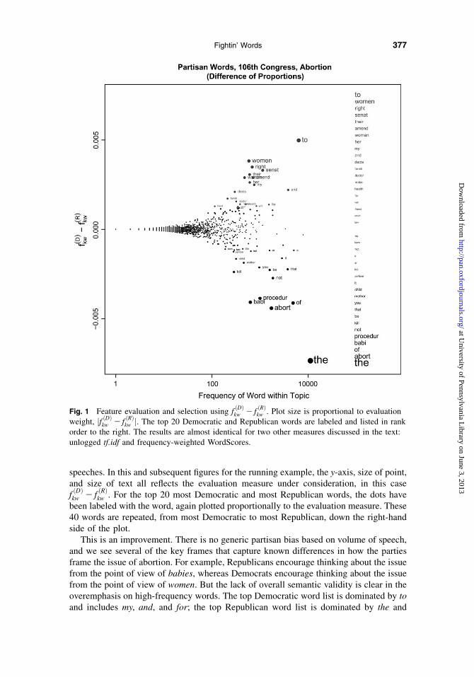
http://www.nytimes.com/interactive/2008/09/04/us/politics/20080905_WORDS_GRAPHIC.html



speeches. In this and subsequent figures for the running example, the y-axis, size of point,and size of text all reflects the evaluation measure under consideration, in this casefðDÞkw 2 f

ðRÞkw . For the top 20 most Democratic and most Republican words, the dots have

been labeled with the word, again plotted proportionally to the evaluation measure. These40 words are repeated, from most Democratic to most Republican, down the right-handside of the plot.

This is an improvement. There is no generic partisan bias based on volume of speech,and we see several of the key frames that capture known differences in how the partiesframe the issue of abortion. For example, Republicans encourage thinking about the issuefrom the point of view of babies, whereas Democrats encourage thinking about the issuefrom the point of view of women. But the lack of overall semantic validity is clear in theoveremphasis on high-frequency words. The top Democratic word list is dominated by toand includes my, and, and for; the top Republican word list is dominated by the and

Fig. 1 Feature evaluation and selection using fðDÞkw 2 f

ðRÞkw . Plot size is proportional to evaluation

weight, jf ðDÞkw 2 fðRÞkw j. The top 20 Democratic and Republican words are labeled and listed in rank

order to the right. The results are almost identical for two other measures discussed in the text:unlogged tf.idf and frequency-weighted WordScores.

377Fightin’ Words



Dow

nloaded from


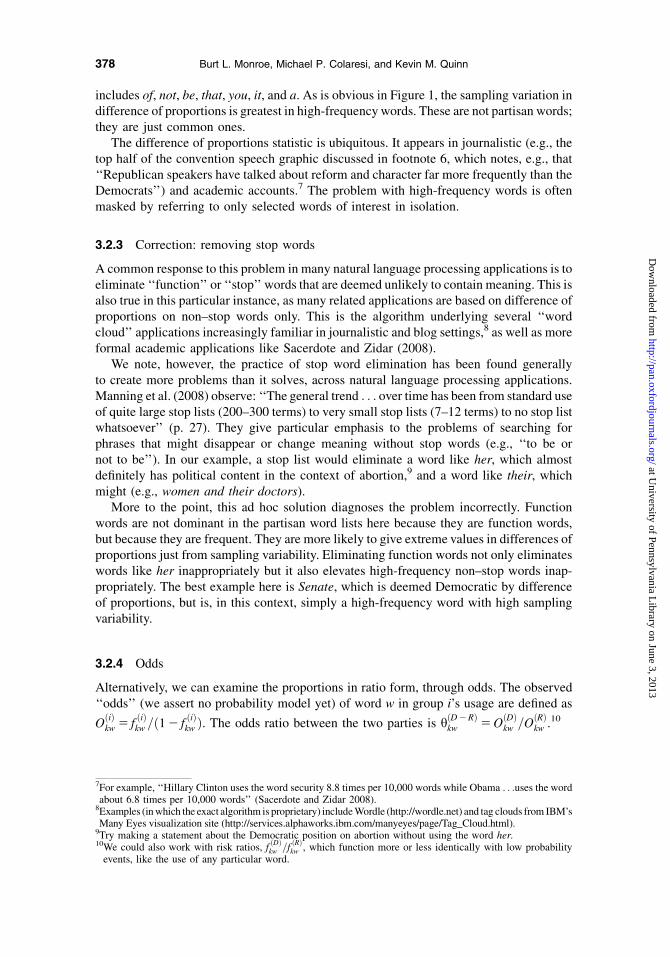
includes of, not, be, that, you, it, and a. As is obvious in Figure 1, the sampling variation indifference of proportions is greatest in high-frequency words. These are not partisan words;they are just common ones.

The difference of proportions statistic is ubiquitous. It appears in journalistic (e.g., thetop half of the convention speech graphic discussed in footnote 6, which notes, e.g., that‘‘Republican speakers have talked about reform and character far more frequently than theDemocrats’’) and academic accounts.7 The problem with high-frequency words is oftenmasked by referring to only selected words of interest in isolation.

3.2.3 Correction: removing stop words

A common response to this problem in many natural language processing applications is toeliminate ‘‘function’’ or ‘‘stop’’ words that are deemed unlikely to contain meaning. This isalso true in this particular instance, as many related applications are based on difference ofproportions on non–stop words only. This is the algorithm underlying several ‘‘wordcloud’’ applications increasingly familiar in journalistic and blog settings,8 as well as moreformal academic applications like Sacerdote and Zidar (2008).

We note, however, the practice of stop word elimination has been found generallyto create more problems than it solves, across natural language processing applications.Manning et al. (2008) observe: ‘‘The general trend . . . over time has been from standard useof quite large stop lists (200–300 terms) to very small stop lists (7–12 terms) to no stop listwhatsoever’’ (p. 27). They give particular emphasis to the problems of searching forphrases that might disappear or change meaning without stop words (e.g., ‘‘to be ornot to be’’). In our example, a stop list would eliminate a word like her, which almostdefinitely has political content in the context of abortion,9 and a word like their, whichmight (e.g., women and their doctors).

More to the point, this ad hoc solution diagnoses the problem incorrectly. Functionwords are not dominant in the partisan word lists here because they are function words,but because they are frequent. They are more likely to give extreme values in differences ofproportions just from sampling variability. Eliminating function words not only eliminateswords like her inappropriately but it also elevates high-frequency non–stop words inap-propriately. The best example here is Senate, which is deemed Democratic by differenceof proportions, but is, in this context, simply a high-frequency word with high samplingvariability.

3.2.4 Odds

Alternatively, we can examine the proportions in ratio form, through odds. The observed‘‘odds’’ (we assert no probability model yet) of word w in group i’s usage are defined as

OðiÞkw 5 f

ðiÞkw =ð12 f

ðiÞkw Þ. The odds ratio between the two parties is hðD2RÞ

kw 5OðDÞkw =O

ðRÞkw .10

7For example, ‘‘Hillary Clinton uses the word security 8.8 times per 10,000 words while Obama . . .uses the wordabout 6.8 times per 10,000 words’’ (Sacerdote and Zidar 2008).

8Examples (in which the exact algorithm is proprietary) include Wordle (http://wordle.net) and tag clouds from IBM’sMany Eyes visualization site (http://services.alphaworks.ibm.com/manyeyes/page/Tag_Cloud.html).

9Try making a statement about the Democratic position on abortion without using the word her.10We could also work with risk ratios, f

ðDÞkw =f

ðRÞkw , which function more or less identically with low probability

events, like the use of any particular word.




Dow

nloaded from

http://wordle.net

http://services.alphaworks.ibm.com/manyeyes/page/Tag_Cloud.html


This is generally presented for single words in isolation or as a metric for ranking words.Examples can be found across the social sciences, including psychology11 and sociology.12

In our data, the odds of a Republican using a variant of babi are 5.4 times those of a Dem-ocratic when talking about abortion, which seems informative. But, the odds of a Repub-lican using the word April are 7.4 times those of a Democrat when talking about abortion,which seems less so.

3.2.5 Log-odds-ratio

Lack of symmetry also makes odds difficult to interpret. Logging the odds ratio providesa measure that is symmetric between the two parties. Working naively, it is unclear what weare to do with words that are spoken by only one party and therefore have infinite oddsratios. If we let the infinite values have infinite weight, the partisan word list consists ofonly those spoken by a single party. The most Democratic words are then bankruptci,Snow½e�, ratifi, confidenti, and church, and the most Republican words are infant, admit,Chines, industri, and 40. If we instead throw out the words with zero counts in one party,the most Democratic words are treati, discrim, abroad, domest, and privacy, and the mostRepublican words are perfect, subsid, percent, overrid, and cell.

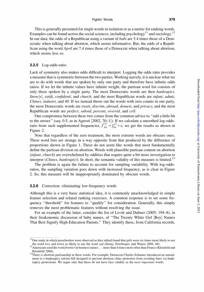
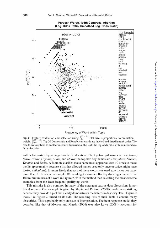
One compromise between these two comes from the common advice to ‘‘add a little bitto the zeroes’’ (say, 0.5, as in Agresti ½2002, 70–1�). If we calculate a smoothed log-odds-ratio from such supplemented frequencies, f

ðiÞkw 5 f

ðiÞkw1e, we get the results as shown in

Figure 2.Note that regardless of the zero treatment, the most extreme words are obscure ones.

These word lists are strange in a way opposite from that produced by the difference ofproportions shown in Figure 1. These do not seem like words that most fundamentallydefine the partisan division on abortion. Words with plausible partisan content on abortion(infant, church) are overwhelmed by oddities that require quite a bit more investigation tointerpret (Chines, bankruptci). In short, the semantic validity of this measure is limited.13

The problem is again the failure to account for sampling variability. With log-odds-ratios, the sampling variation goes down with increased frequency, as is clear in Figure2. So, this measure will be inappropriately dominated by obscure words.

3.2.6 Correction: eliminating low-frequency words

Although this is a very basic statistical idea, it is commonly unacknowledged in simplefeature selection and related ranking exercises. A common response is to set some fre-quency ‘‘threshold’’ for features to ‘‘qualify’’ for consideration. Generally, this simplyremoves the most problematic features without resolving the issue.

For an example of the latter, consider the list of Levitt and Dubner (2005; 194–8), intheir freakonomic discussion of baby names, of ‘‘The Twenty White Girl ½Boy� NamesThat Best Signify High-Education Parents.’’ They identify these, from California records,

11One study in which preschoolers were observed as they talked found that girls were six times more likely to usethe word love and twice as likely to use the word sad (Senay, Newberger, and Waters 2004, 68).

12Americans used the word frontier in business names . . .more than 4 times more often than France (Kleinfeld andKleinfeld 2004).

13There is abortion partisanship in these words. For example, Democrat Charles Schumer introduced an amend-ment to a bankruptcy reform bill designed to prevent abortion clinic protesters from avoiding fines via bank-ruptcy protections. We argue only that these do not have face validity as the most important words.

379Fightin’ Words



Dow

nloaded from


with a list ranked by average mother’s education. The top five girl names are Lucienne,Marie-Claire, Glynnis, Adair, and Meira; the top five boy names are Dov, Akiva, Sander,Yannick, and Sacha. A footnote clarifies that a name must appear at least 10 times to makethe list (presumably because a list that allowed names used only once or twice might havelooked ridiculous). It seems likely that each of these words was used exactly, or not manymore than, 10 times in the sample. We would get a similar effect by drawing a line at 10 or100 minimum uses of a word in Figure 2, with the method then selecting the most extremeexamples from the least frequent qualifying words.

This mistake is also common in many of the emergent text-as-data discussions in po-litical science. One example is given by Slapin and Proksch (2008), made more strikingbecause they provide a plot that clearly demonstrates the heteroskedasticity. Their Figure 2looks like Figure 2 turned on its side. The resulting lists of their Table 1 contain manyobscurities. This is probably only an issue of interpretation. The item response model theydescribe, like that of Monroe and Maeda (2004) (see also Lowe ½2008�), accounts for

Fig. 2 Feature evaluation and selection using dðD2RÞkw . Plot size is proportional to evaluation

weight,��dðD2RÞ

kw j. Top 20 Democratic and Republican words are labeled and listed in rank order. Theresults are identical to another measure discussed in the text: the log-odds-ratio with uninformativeDirichlet prior.




Dow

nloaded from


variance when the word parameters are used to estimate speaker/author positions. That is,despite their use of captions like ‘‘word weights’’ and ‘‘Top Ten Words placing parties onthe left and right,’’ these are really the words with the 10 leftmost and rightmost pointestimates, not the words that have the most influence in the estimates of actor positions.

3.2.7 tf.idf (Computer Science)

It is common practice in the computational linguistics applications of classification (e.g.,Which bin does this document belong in?) and search (e.g., Which document(s) should thisset of terms be matched to?) to model documents not by their words but by words that havebeen weighted by their tf.idf, or term frequency—inverse document frequency. Term fre-quency refers to the relative frequency (proportion) with which a word appears in the doc-ument; document frequency refers to the relative frequency with which a word appears, atall, in documents across the collection. The logic of tf.idf is that the words containing thegreatest information about a particular document are the words that appear many times inthat document, but in relatively few others. tf.idf is recommended in standard textbooks(Jurafsky and Martin (2000, 651–4) (Manning and Schutze 1999, 541–4) and is widelyused in document search and information retrieval tasks.14 To the extent tf.idf reliably cap-tures what is distinctive about a particular document, it could be interpreted as a featureevaluation technique.

The most common variant of tf.idf logs the idf term—this is the ‘‘ntn’’ variant (naturaltf term, logged df term, no normalization, see Manning and Schutze ½1999, 544�). So, lettingdfkw denote the fraction of groups that use the word w on topic k at least once, then:

tf :idfðiÞkw ðntnÞ5 f ikwln ð1=dfkwÞ: ð1Þ

Qualitatively, the results from this approach are identical to the infinite log-odds-ratioresults given earlier. The most partisan words are the words spoken the most by one party,while spoken not once by the other (bankruptci, infant).15 Clearly, the logic of logging thedocument frequency16 breaks down in a collection of two documents.

Alternatively, we can use an unlogged document frequency term—the ‘‘nnn’’ (natural tfterm, natural df term, no normalization; see Manning and Schutze ½1999, 544�) variant oftf.idf.

tf :idfðiÞkw ðnnnÞ5 f ikw =dfkw: ð2Þ

The results for our running example are nearly identical, qualitatively and quantitativelywith those from raw difference of proportions, shown in Figure 1. The weights are cor-related (at 10.997 in this case) and differ only in doubling the very low weights of therelatively low-frequency words used by only one party.17 In any case, for our purposes,neither version of tf.idf has clear value. See Hiemstra (2000) and Aizawa (2003) for effortsto put tf.idf on a probabilistic or information-theoretic footing.

14We note over 15,000 hits for the term in Google Scholar.15The degenerate graphic of this result is omitted for space reasons, but available in the web appendix.16Due to the large number of documents in many collections, this measure is usually squashed with a log function

(Jurafsky and Martin 2000, 653).17We omit this mostly redundant graphic here. It is available in the web appendix.

381Fightin’ Words



Dow

nloaded from


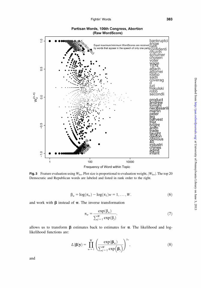
3.2.8 WordScores (Political Science)

Perhaps the most prominent text-as-data approach in political science is the WordScoresprocedure (Laver et al. 2003), which embeds a feature evaluation technique in its algo-rithm. The first step of the algorithm establishes scores for words based on their frequencieswithin ‘‘reference’’ texts, which are then used to scale other ‘‘virgin’’ texts (for furtherdetail, see Lowe ½2008�).

In our running example, we calculate these by setting the Democrats at 11 and theRepublicans at 21. Then the raw WordScore for each word is:

WðD2RÞkw 5

yðDÞkw =n

ðDÞk 2 y

ðRÞkw =n

ðRÞk

yðDÞkw =n

ðDÞk 1 y

ðRÞkw =n

ðRÞk

: ð3Þ

Figure 3 shows the results of applying this stage of the WordScores algorithm to our run-ning example. The results bear qualitative resemblance to those with the smoothed log-odds-ratios shown in Figure 2. As shown in Figure 3, the extreme Wkw are received by thewords spoken by only one party. As with several previous measures, the maximal words areobscure low-frequency words.

The ultimate use for WordScores, however, is for the spatial placement of documents.When the Wkw are taken forward to the next step, the impact of any word is proportional toits relative frequency. That is, the implicit evaluation measure, W

�ðD2RÞkw , is

W�ðD2RÞkw 5

yðDÞkw =n

ðDÞk 2 y

ðRÞkw =n

ðRÞk

yðDÞkw =n

ðDÞk 1 y

ðRÞkw =n

ðRÞk

nkw: ð4Þ

In the case of two ‘‘documents,’’ as is the case here, this is nearly identical to the differenceof proportions measure. In this example, they correlate at over 10.998. So, WordScoresdemonstrates the same failure to account for sampling variation and the same overweight-ing of high-frequency words. Lowe (2008) (in this volume) gives much greater detail on theworkings of the WordScores procedure and how it might be given a probabilistic footing.

3.3 Model-Based Approaches

In our preferred model-based approaches, we model the choice of word as a function ofparty, P(wjp). We begin by discussing a model for the full collection of documents and thenshow how this can be used as a starting point and baseline for subgroup-specific models. Ingeneral, our strategy is to first model word usage in the full collection of documents and tothen investigate how subgroup-specific word usage diverges from that in the full collectionof documents.

3.3.1 The likelihood

Consider the following model. We will start without subscripts and consider the counts inthe entire corpus, y:

y�Multinomialðn;pÞ; ð5Þ

where n 5PW

w5 1 yw and p is a W-vector of multinomial probabilities. Since p is a vectorof multinomial probabilities, it is constrained to be in the (W 2 1)–dimensional simplex. Insome variants below, we reparameterize and use the (unbounded) log odds transformation




Dow

nloaded from


bw 5 logðpwÞ2 logðp1Þw5 1; . . . ;W: ð6Þ

and work with b instead of p. The inverse transformation

pw 5expðbwÞPWj5 1 expðbjÞ

: ð7Þ

allows us to transform b estimates back to estimates for p. The likelihood and log-likelihood functions are:

LðbjyÞ5YWw5 1

expðbwÞPWj5 1 exp

�bj

�!yw

; ð8Þ

and

Fig. 3 Feature evaluation using Wkw. Plot size is proportional to evaluation weight, jWkwj. The top 20Democratic and Republican words are labeled and listed in rank order to the right.

383Fightin’ Words



Dow

nloaded from


‘ðbjyÞ5XWw5 1

ywlog

expðbwÞPWj5 1 exp

�bj

�!: ð9Þ

Within any topic, k, the model to this point goes through with addition of subscripts:

yk �Multinomialðnk;pkÞ; ð10Þ

with parameters of interest, bkw, and log-likelihood, ‘ðbkjykÞ, defined analogously.Further, within any group-topic partition, indexed by i and k, we superscript for group to

model:

yðiÞk �Multinomial

�nðiÞk ;p

ðiÞk

�; ð11Þ

with parameters of interest, bðiÞkw, and log-likelihood, ‘ðbðiÞk jyðiÞk Þ, defined analogously.

If we wish to proceed directly to ML estimation, the lack of covariates results in animmediately available analytical solution for the MLE of bðiÞkw. We calculate

pMLE 5 f5 y � ð1=nÞ; ð12Þ

and bMLE

follows after transforming.

3.3.2 Prior

The simplest Bayesian model proceeds by specifying the prior using the conjugate for themultinomial distribution, the Dirichlet:

p�DirichletðaÞ; ð13Þ

where a is a W-vector, aw > 0, with a very clean interpretation in terms of ‘‘prior samplesize.’’ That is, use of any particular Dirichlet prior defined by a affects the posterior exactlyas if we had observed in the data an additional aw – 1 instances of word w. This can bearbitrarily uninformative, for example, aw 5 0.01 for all w. Again, we can carry this modelthrough to topics and topic-group partitions with appropriate sub- and superscripting.

3.3.3 Estimation

Due to the conjugacy, the full Bayesian estimate using the Dirichlet prior is also analyt-ically available in analogous form:

p5�y1a

�� 1��

n1 a0�: ð14Þ

where a0 5PW

w5 1 aw.Again, all this goes directly through to partitions with appropriate subscripts if desired.

3.3.4 Feature evaluation

What we have to this point is sufficient to suggest the first approach to feature evaluation.Denote the odds (now with probabilistic meaning) of word w, relative to all others, as




Dow

nloaded from


Xw 5 pw/(1 – pw), again with additional sub- and superscripts for specific partitions. Sincethe Xw are functions of the pw, estimates of these follow directly from the pw.

Within any one topic, k, we are interested in how the usage of a word by group i differsfrom usage of the word in the topic by all groups, which we can capture with the log-odds-ratio, which we will now define as dðiÞw 5 logðXðiÞ

w =XwÞ. The point estimate for this is

dðiÞkw 5 log

h �yðiÞkw 1 aðiÞkw

��nðiÞk 1 aðiÞk0 2 y

ðiÞkw 2 aðiÞkw

�i2 log

�ðykw 1 akwÞ

ðnk 1 ak0 2 ykw 2 akwÞ

�: ð15Þ

In certain cases, we may be more interested in the comparison of two specific groups. Thisis the case in our running example, where we will have exactly two groups, Democrats andRepublicans. The usage difference is then captured by the log-odds-ratio between the twogroups, dði2 jÞ

w , which is estimated by

dði2 jÞkw 5 log

h �yðiÞkw 1 aðiÞkw

��nðiÞk 1 aðiÞk0 2 y

ðiÞkw 2 aðiÞkw

�i2 logh �

yðjÞkw 1 aðjÞkw

��nðjÞk 1 aðjÞk0 2 y

ðjÞkw 2 aðjÞkw

�i: ð16Þ

Without the prior, this is of course simply the observed log-odds-ratio. This would emergefrom viewing word counts as conventional categorical data in a contingency table or a logit.For each word, imagine a 2 � 2 contingency table, with the cells including the counts, foreach of the two groups, of word w and of all other words. Or, we can specify a logit of thebinary choice, word w versus any other word, with our party group indicator the only re-gressor. With more than two groups, the same information, with slightly more manipula-tion (via risk ratios), can be recovered from a multinomial logit or an appropriatelyconstrained Poisson regression (Agresti 2002). With the prior, this is a relabeling ofthe smoothed log-odds-ratio discussed before.

So, if we apply the measure, with equivalent prior, we get results identical to thoseshown in Figure 2. This has the same problems, with the dominant words still the samelist of obscurities. The problem is clearly that the estimates for infrequently spoken wordshave higher variance than frequently spoken ones.

We can now exploit the first advantage of having specified a model. Under the givenmodel, the variance of these estimates is approximately:

r2

dðiÞkw

� 1�

yðiÞkw 1 aðiÞkw

�1 1�nðiÞk 1 aðiÞk0 2 y

ðiÞkw 2 aðiÞkw

�1 1

ðykw 1 akwÞ1

1

ðnk 1 ak0 2 ykw 2 akwÞ;

ð17Þ

� 1�yðiÞkw 1 aðiÞkw

�1 1

ðykw 1 akwÞ; ð18Þ

and

r2�dði2 jÞkw

�� 1�

yðiÞkw1aðiÞkw

�1 1�nðiÞk 1aðiÞk02y

ðiÞkw2aðiÞkw

�1 1�yðjÞkw1aðjÞkw

�1 1�nðjÞk 1aðjÞk02y

ðjÞkw2aðjÞkw

�;ð19Þ

385Fightin’ Words



Dow

nloaded from


� 1�yðiÞkw 1 aðiÞkw

�1 1�yðjÞkw 1 aðjÞkw

�: ð20Þ

Where the approximations in Equations 17 and 19 assume yðiÞkw � aðiÞkw; ykw � akw and

ignore covariance terms that will typically be close to 0 while Equations 18 and 20 ad-ditionally assume that n

ðiÞk � y

ðiÞkw and nk � ykw. The approximations are unnecessary but

reasonable for documents of moderate size (at 1000 words only the fourth decimal place isaffected) and help clarify the variance equation. Variance is based on the absolute fre-quency of a word in all, or both, documents of interest, and its implied absolute frequencyin the associated priors.

3.4 Accounting for Variance

Now we can evaluate features not just by their point estimates but also by our certaintyabout those estimates. Specifically, we will use as the evaluation measure the z-scores of thelog-odds-ratios, which we denote with f:

fðiÞkw 5 d

ðiÞkw=

ffiffiffiffiffiffiffiffiffiffiffiffiffiffiffiffiffiffir2�dðiÞkw

�r; ð21Þ

and

fði2 jÞkw 5 d

ði2 jÞkw =

ffiffiffiffiffiffiffiffiffiffiffiffiffiffiffiffiffiffiffiffiffiffir2�dði2 jÞkw

�r: ð22Þ

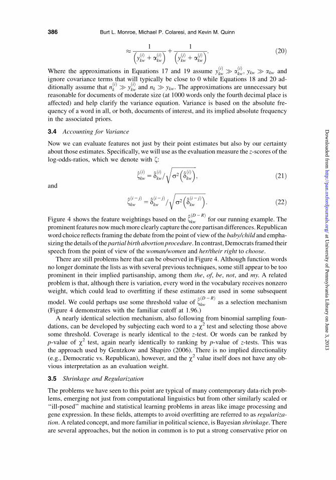
Figure 4 shows the feature weightings based on the fðD2RÞkw for our running example. The

prominent features now much more clearly capture the core partisan differences. Republicanword choice reflects framing the debate from the point of view of the baby/child and empha-sizing the details of the partial birth abortion procedure. In contrast, Democrats framed theirspeech from the point of view of the woman/women and her/their right to choose.

There are still problems here that can be observed in Figure 4. Although function wordsno longer dominate the lists as with several previous techniques, some still appear to be tooprominent in their implied partisanship, among them the, of, be, not, and my. A relatedproblem is that, although there is variation, every word in the vocabulary receives nonzeroweight, which could lead to overfitting if these estimates are used in some subsequent

model. We could perhaps use some threshold value of fðD2RÞkw as a selection mechanism

(Figure 4 demonstrates with the familiar cutoff at 1.96.)A nearly identical selection mechanism, also following from binomial sampling foun-

dations, can be developed by subjecting each word to a v2 test and selecting those abovesome threshold. Coverage is nearly identical to the z-test. Or words can be ranked byp-value of v2 test, again nearly identically to ranking by p-value of z-tests. This wasthe approach used by Gentzkow and Shapiro (2006). There is no implied directionality(e.g., Democratic vs. Republican), however, and the v2 value itself does not have any ob-vious interpretation as an evaluation weight.

3.5 Shrinkage and Regularization

The problems we have seen to this point are typical of many contemporary data-rich prob-lems, emerging not just from computational linguistics but from other similarly scaled or‘‘ill-posed’’ machine and statistical learning problems in areas like image processing andgene expression. In these fields, attempts to avoid overfitting are referred to as regulariza-tion. A related concept, and more familiar in political science, is Bayesian shrinkage. Thereare several approaches, but the notion in common is to put a strong conservative prior on




Dow

nloaded from


the model. We bias the model toward the conclusion of no partisan differences, requiringthe data to speak very loudly if such a difference is to be declared.

In this section, we discuss two approaches. In the first, we use the same model as above,but put considerably more information into the Dirichlet prior. In the second, we use a dif-ferent (Laplace) functional form for the prior distribution.

3.5.1 Informative Dirichlet prior

One approach is to use more of what we know about the expected distribution of words. We cando this by specifying a prior proportional to the expected distribution of features in a randomtext. That is, we know the is used much more often than nuclear, and our prior can reflectthat information. In our running example, we can use the observed proportion of words inthe vocabulary in the context of Senate speech, but across multiple Senate topics.18 That is,

Fig. 4 Feature evaluation and selection using fðD2RÞkw . Plot size is proportional to evaluation weight,��fðD2RÞ

kw

��; those with��fðD2RÞ

kw

��<1:96 are gray. The top 20 Democratic and Republican words are

labeled and listed in rank order to the right.

18Although this is technically not a legitimate subjective prior because the data are being used twice, nearly all theprior information is coming from data that are not used in the analysis. Qualitatively similar empirical Bayesresults could be obtained by basing the prior on speeches on all topics other than the topic in question or, for thatmatter, on general word frequency information from other sources altogether.

387Fightin’ Words



Dow

nloaded from


aðiÞkw 5 aðiÞk0pMLE 5 y � a0

nð23Þ

where aðiÞk0 determines the implied amount of information in the prior. This prior shrinks thepðiÞkw and XðiÞ

kw to the global values, and shrinks the feature evaluation measures, the fðiÞkw andthe fði2 jÞ

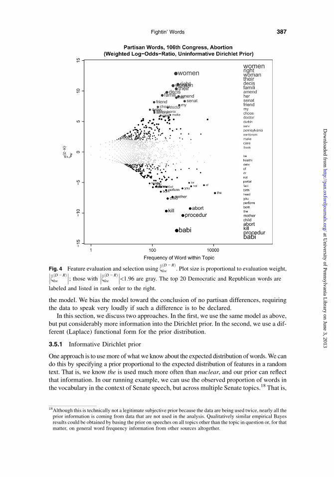
kw , toward zero. The greater aðiÞk0 is, the more shrinkage we will have.Figure 5 illustrates results from the running example using this approach. We set a0 to

imply a ‘‘prior sample’’ of 500 words per party every day, roughly the average number ofwords per day used per party on each topic in the data set.

As is shown in Figure 5, this has a desirable effect on the function-word problem notedabove. For example, the Republican top 20 list has shuffled, with the, you, not, of, and bebeing replaced by the considerably more evocative aliv, infant, brutal, brain, and necessari.

Fig. 5 Feature evaluation and selection based on fðD2RÞkw . Plot size is proportional to evaluation

weight, fðD2RÞkw ; those with

��fðD2RÞkw

��<1:96 are gray. The top 20 Democratic and Republican words are

labeled and listed in rank order to the right.




Dow

nloaded from


We also see an apparent improvement in selection, with fewer words now exceeding thesame f threshold.

The amount of shrinkage is determined by the scale parameter in the Dirichlet priorrelative to the absolute frequency of speech in the topic. The prior used in this examplehas almost no effect on estimates in topics with much more speech and strong partisandifferences (like defense, post-Iraq), and overwhelms estimates—as it should—in topicswith very little speech or no partisan differences (like symbolic constituent tributes).

Relative to the technique in the next section, this simple approach has several advan-tages. First, because of the analytical solution, it requires very little computation. Second,this low computational overhead makes it relatively straightforward to develop more flex-ible variants, such as a dynamic version we discuss below. Third, the fact that these esti-mates could be recovered from appropriate standard Bayesian generalized linear modelsmeans the approach is easily extended beyond the setting of a strict partitioning of thedocument space into discrete groups. Multiple observable characteristics (party *and* gen-der *and* geographic district) can be modeled simultaneously, subject to the identificationconstraints typical of a regression problem.

This approach still suffers as a technique for feature selection: it is unclear where onedraws the line between words that qualitatively matter and words that qualitatively do not.So, there is still the problem for the qualitative analyst of interpreting a long (weighted/ordered) list and the problem for the quantitative analyst of possibly overfitting if these areused in subsequent modeling.

3.5.2 Laplace prior

We address this here by using an alternative functional form for the prior, one which shrinksmost contrasts between estimates not toward zero, but to zero. In this approach, we specifya prior for b

ðiÞk . Specifically, we assume

bðiÞind:kw� LaplaceðbMLE

kw ; cÞ; w5 2; . . . ;W: ð24Þ

Or, even more precisely,

pðbðiÞk jcÞ5

YWw5 2

c2exp�2 c��bðiÞkw 2 b

MLE

kw

��: ð25Þ

Here bMLEk is the maximum likelihood estimate from an analysis of the pooled y which

serves as the ‘‘prior’’ mode for bðiÞk and c > 0 serves as an inverse scale parameter.It is fairly well known that such a prior is equivalent to an L1 regularization penalty

(Williams 1995). In practice, such a prior (or regularization penalty) causes many, ifnot most, of the elements of the posterior mode of b

ðiÞk to be exactly equal to the prior

mode bMLE

k .To finish the prior specification, we consider two types of hyper-priors for c. The first is

that c follows an exponential distribution.

pEðcÞ5 a expð2 acÞ: ð26Þ

The second is the improper Jeffreys prior:

pJðcÞ} 1=c: ð27Þ

389Fightin’ Words



Dow

nloaded from


It is well known that this corresponds to a uniform prior for log(c).Under the exponential hyper-prior for c, the full posterior becomes:

pðbðiÞk ; cjyðiÞk Þ} pðyðiÞk jbðiÞ

k ÞpðbðiÞk jcÞpEðcÞ

}

(YWw5 1

expðbðiÞkwÞPW

i5 1

expðbðiÞki Þ

!ykw)(YWw5 2


MLE

kw

��)aexp

�2 ac

�ð28Þ

and under the Jeffreys hyper-prior for c, the full posterior becomes:


k ÞpðbðiÞk jcÞpJðcÞ

}

(YWw5 1

expðbðiÞkwÞPW

i5 1

exp

bðiÞki

!ykw)(YW

i5 2


MLE

kw

��)1�c: ð29Þ

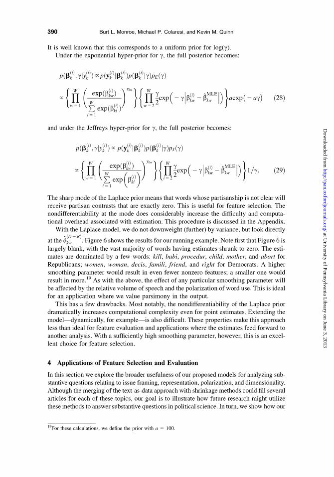
The sharp mode of the Laplace prior means that words whose partisanship is not clear willreceive partisan contrasts that are exactly zero. This is useful for feature selection. Thenondifferentiability at the mode does considerably increase the difficulty and computa-tional overhead associated with estimation. This procedure is discussed in the Appendix.

With the Laplace model, we do not downweight (further) by variance, but look directly

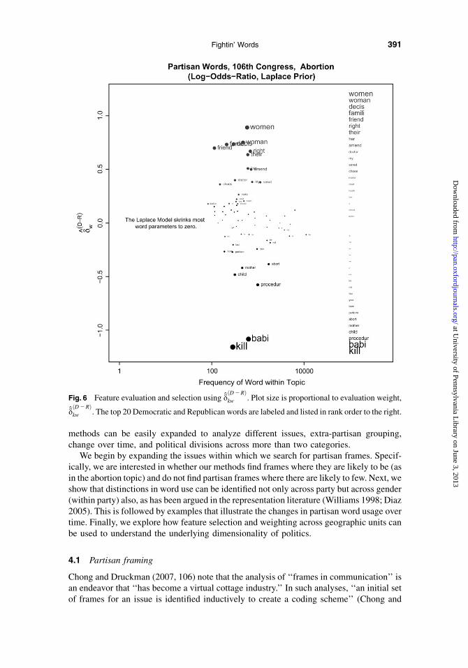
at the dðD2RÞkw . Figure 6 shows the results for our running example. Note first that Figure 6 is

largely blank, with the vast majority of words having estimates shrunk to zero. The esti-mates are dominated by a few words: kill, babi, procedur, child, mother, and abort forRepublicans; women, woman, decis, famili, friend, and right for Democrats. A highersmoothing parameter would result in even fewer nonzero features; a smaller one wouldresult in more.19 As with the above, the effect of any particular smoothing parameter willbe affected by the relative volume of speech and the polarization of word use. This is idealfor an application where we value parsimony in the output.

This has a few drawbacks. Most notably, the nondifferentiability of the Laplace priordramatically increases computational complexity even for point estimates. Extending themodel—dynamically, for example—is also difficult. These properties make this approachless than ideal for feature evaluation and applications where the estimates feed forward toanother analysis. With a sufficiently high smoothing parameter, however, this is an excel-lent choice for feature selection.

4 Applications of Feature Selection and Evaluation

In this section we explore the broader usefulness of our proposed models for analyzing sub-stantive questions relating to issue framing, representation, polarization, and dimensionality.Although the merging of the text-as-data approach with shrinkage methods could fill severalarticles for each of these topics, our goal is to illustrate how future research might utilizethese methods to answer substantive questions in political science. In turn, we show how our

19For these calculations, we define the prior with a 5 100.




Dow

nloaded from


methods can be easily expanded to analyze different issues, extra-partisan grouping,change over time, and political divisions across more than two categories.

We begin by expanding the issues within which we search for partisan frames. Specif-ically, we are interested in whether our methods find frames where they are likely to be (asin the abortion topic) and do not find partisan frames where there are likely to few. Next, weshow that distinctions in word use can be identified not only across party but across gender(within party) also, as has been argued in the representation literature (Williams 1998; Diaz2005). This is followed by examples that illustrate the changes in partisan word usage overtime. Finally, we explore how feature selection and weighting across geographic units canbe used to understand the underlying dimensionality of politics.

4.1 Partisan framing

Chong and Druckman (2007, 106) note that the analysis of ‘‘frames in communication’’ isan endeavor that ‘‘has become a virtual cottage industry.’’ In such analyses, ‘‘an initial setof frames for an issue is identified inductively to create a coding scheme’’ (Chong and

Fig. 6 Feature evaluation and selection using dðD2RÞkw . Plot size is proportional to evaluation weight,

dðD2RÞkw . The top 20 Democratic and Republican words are labeled and listed in rank order to the right.

391Fightin’ Words



Dow

nloaded from


Druckman 2007, 107). The result of this initial stage is something like the 65-argumentcoding scheme developed by Baumgartner et al. (2008) to exhaustively capture the pro-and antiframes used in debate over the death penality (Baumgartner et al. 2008, 103–12,243–51). These then serve as the basis for a content analysis of relevant texts, like news-paper articles, to evaluate variations in frame across source and across time. The featureselection techniques we describe here can be useful for such a purpose.

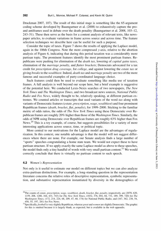
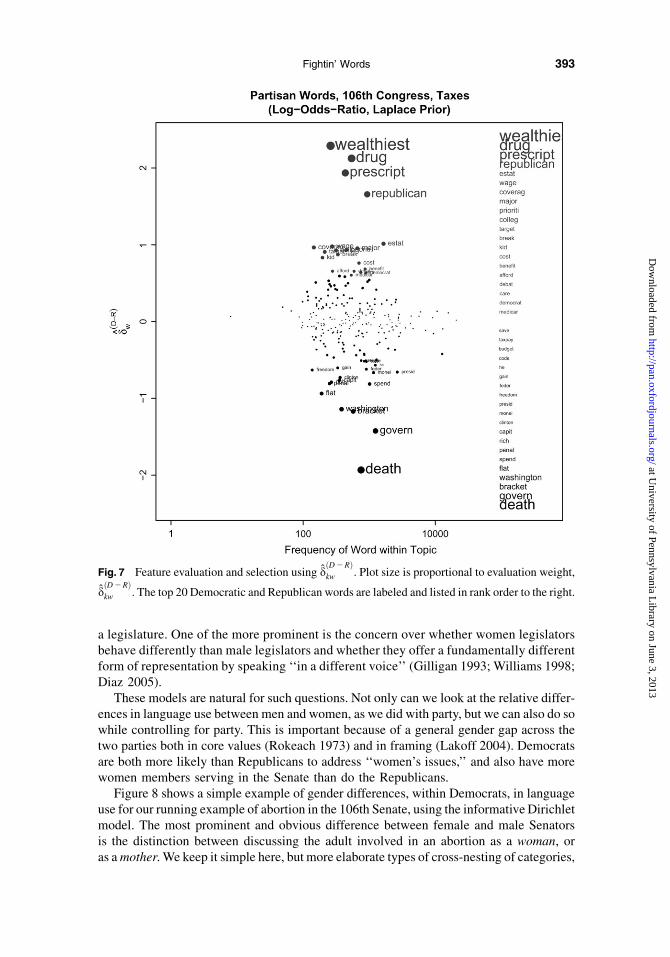
Consider the topic of taxes. Figure 7 shows the results of applying the Laplace model,again in the 106th Congress. Note the more compressed y-axis, relative to the abortionanalysis of Figure 6, indicating that during this period taxation was a considerably morepartisan topic. The prominent features identify the most prominent partisan frames. Re-publicans were pushing for elimination of the death tax, lowering of capital gains taxes,elimination of the marriage penalty, and flatter brackets; Democrats advocated for a taxcredit for prescription drug coverage, for college, and against lowering the estate tax orgiving breaks to the wealthiest. Indeed, death tax and marriage penalty are two of the morefamous and successful examples of party-coordinated language choice.

Such features could then be used to evaluate something like media use of taxationframes. A full analysis is well beyond our scope here, but a brief example is suggestiveof the potential here. We conducted Lexis-Nexis searches of two newspapers, The NewYork Times and The Washington Times, and two broadcast news sources, National PublicRadio and Fox News, widely thought to be, relatively speaking, at different partisan ex-tremes. We counted articles or transcripts that used variants of the word tax along withvariants of Democratic features (estate, prescription, wage, wealthiest) and four prominentRepublican frames (death, bracket, flat, penalty), for 1999–2000. Sticking to the familiarmetric of odds ratios, the odds of The New York Times using these Democratic over Re-publican frames are roughly 20% higher than those of the Washington Times. Similarly, theodds of NPR using Democratic over Republican frames are roughly 63% higher than FoxNews.20 This is a toy example, of course, but suggests possibilities for a variety of moreinteresting applications across source, time, or political topic.

More central to our motivations for the Laplace model are the advantages of regula-rization. In this context, one notable advantage is that the model will not suggest differ-ences where there are none. For example, our Senate analysis finds a large number of‘‘sports’’ speeches congratulating a home state team. We would not expect these to havepartisan structure. If we apply exactly the same Laplace model as above to these speeches,the model finds only a tiny handful of words with very small partisan content.21 We wouldcorrectly conclude that there is virtually no partisan content to such speech.

4.2 Women’s Representation

Not only is it useful to estimate our model on different topics but we can also analyzeextra-partisan distinctions. For example, a long-standing question in the representationliterature concerns the relative roles of descriptive representation, symbolic representa-tion, and substantive representation instantiated by diversity in the demographics of

20The counts of estate, prescription, wage, wealthiest, death, bracket, flat, penalty, respectively, are (2078, 620,1159, 208, 1280, 164, 431, 743) for The New York Times, (1032, 376, 692, 84, 731, 189, 399, 720) for TheWashington Times, (172, 214, 224, 68, 209, 47, 68, 174) for National Public Radio, and (167, 362, 238, 54,450, 55, 197, 281) for Fox News.

21Specifically, football is very slightly Republican, whereas great and women are slightly Democratic. The graphicfor this is omitted because it is largely blank, as expected, but is available in the web appendix.




Dow

nloaded from


a legislature. One of the more prominent is the concern over whether women legislatorsbehave differently than male legislators and whether they offer a fundamentally differentform of representation by speaking ‘‘in a different voice’’ (Gilligan 1993; Williams 1998;Diaz 2005).

These models are natural for such questions. Not only can we look at the relative differ-ences in language use between men and women, as we did with party, but we can also do sowhile controlling for party. This is important because of a general gender gap across thetwo parties both in core values (Rokeach 1973) and in framing (Lakoff 2004). Democratsare both more likely than Republicans to address ‘‘women’s issues,’’ and also have morewomen members serving in the Senate than do the Republicans.

Figure 8 shows a simple example of gender differences, within Democrats, in languageuse for our running example of abortion in the 106th Senate, using the informative Dirichletmodel. The most prominent and obvious difference between female and male Senatorsis the distinction between discussing the adult involved in an abortion as a woman, oras a mother. We keep it simple here, but more elaborate types of cross-nesting of categories,

Fig. 7 Feature evaluation and selection using dðD2RÞkw . Plot size is proportional to evaluation weight,

dðD2RÞkw . The top 20 Democratic and Republican words are labeled and listed in rank order to the right.

393Fightin’ Words



Dow

nloaded from


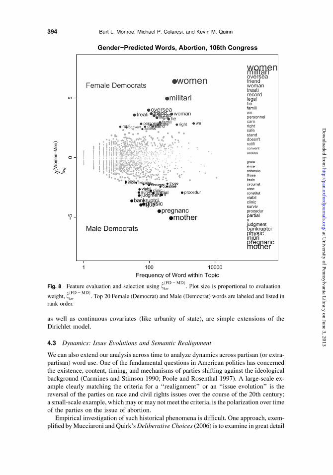
as well as continuous covariates (like urbanity of state), are simple extensions of theDirichlet model.

4.3 Dynamics: Issue Evolutions and Semantic Realignment

We can also extend our analysis across time to analyze dynamics across partisan (or extra-partisan) word use. One of the fundamental questions in American politics has concernedthe existence, content, timing, and mechanisms of parties shifting against the ideologicalbackground (Carmines and Stimson 1990; Poole and Rosenthal 1997). A large-scale ex-ample clearly matching the criteria for a ‘‘realignment’’ or an ‘‘issue evolution’’ is thereversal of the parties on race and civil rights issues over the course of the 20th century;a small-scale example, which may or may not meet the criteria, is the polarization over timeof the parties on the issue of abortion.

Empirical investigation of such historical phenomena is difficult. One approach, exem-plified by Mucciaroni and Quirk’s Deliberative Choices (2006) is to examine in great detail

Fig. 8 Feature evaluation and selection using fðFD2MDÞkw . Plot size is proportional to evaluation

weight, fðFD2MDÞkw . Top 20 Female (Democrat) and Male (Democrat) words are labeled and listed in

rank order.




Dow

nloaded from


the traceable behaviors—in this case, Congressional speeches, testimony, etc.—for a par-ticular policy debate held over a relatively short time scale. A second approach, exempli-fied by Carmine and Stimson’s Issue Evolution (1990) and similar work that followed itslead (Adams 1997), looks for changes across more abstract traceable behaviors—for ex-ample, rollcall votes in Congress, survey responses—in a single issue area over a long timescale: race for Carmines and Stimson, abortion and others for later work. A third approach,exemplified by Poole and Rosenthal’s Congress (1997), looks at a single behavior—Congressional rollcall votes—across all issues and long time scales, looking for abstractchanges in the partisan relationship, such as the dimensionality of a model required toexplain the behaviors.

Speech offers interesting potential leverage on the problem. We have seen that staticsnapshots can illuminate the content of a particular partisan conflict. If these techniques canbe extended dynamically, we can look directly at how the content of partisan conflictchanges.

The analytic solution of the Dirichlet model makes dynamic extensions straightforward.First, the y are extremely noisy on a day-to-day basisso we apply a smoother to the data.22

Then we calculate zeta over a moving time window of the data.A genuine partisan realignment or issue evolution would be evidenced by massive shifts

in the partisanship of language. That is, a necessary condition for an issue evolution wouldbe for some words to switch sides, to flip sign in our measure. This generally occurred (orbeen agreed to have occurred) only over fairly long time frames. So, over the relativelyshort time frame of these data, 8 years, we would not expect to find much that would qualifyas such. However, we do find many microscale movements that suggest such analyses canprove fruitful.

For example, we find several instances where Republicans ‘‘own’’ an issue or framewhile in opposition to Clinton are successful in obtaining a policy change during the Bushhoneymoon period of early 2001 or in the rally period after 9/11, only to find Democrats‘‘owning’’ the issue when the policy becomes unpopular. Dramatic examples include debtwhen discussing the budget, oil when discussing energy policy, and Iraq when discussingdefense policy.

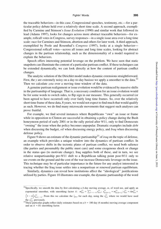
Figure 9 shows an estimate of the dynamic partisanship23 of iraq on the topic of defense,an example which provides a unique window into the dynamics of partisan conflict. Inorder to observe shifts in the tectonic plates of partisan conflict, we need both salience(the parties and presumably the public must care) and some exogenous shock or changein the status quo (to motivate change). Iraq supplies both of these, and in turn, we seerelative nonpartisanship pre-9/11 shift to a Republican talking point post-9/11 only tosee events on the ground and the cost of the war increase Democratic leverage on the issue.This technique may be of particular importance in the future for any analyst interested intracing whether the Iraq issue settles into a nonpartisan or renewed partisan equilibrium.

Similarly, dynamics can reveal how institutions affect the ‘‘ideological’’ justificationsutilized by parties. Figure 10 illustrates one example, the dynamic partisanship of the word

22Specifically, we smooth the data by first calculating a b-day moving average, m, of word use, and apply an

exponential smoother, with smoothing factor A : mðiÞkwt 5

Pts5 t2 b y

ðiÞkws; s

ðiÞkwðb11Þ 5m

ðiÞkwðb11Þ; s

ðiÞkwt 5Am

ðiÞkwt1�

12A�sðiÞkwðt2 1Þ. From this we calculate the fkwt for each day, using the s

ðiÞkwt where we would have used

the yðiÞkwt previously.

23These particular graphs reflect daily estimates based on a b 5 180 day (6 months) moving average componentand an A 5.01 smoothing factor.

395Fightin’ Words



Dow

nloaded from


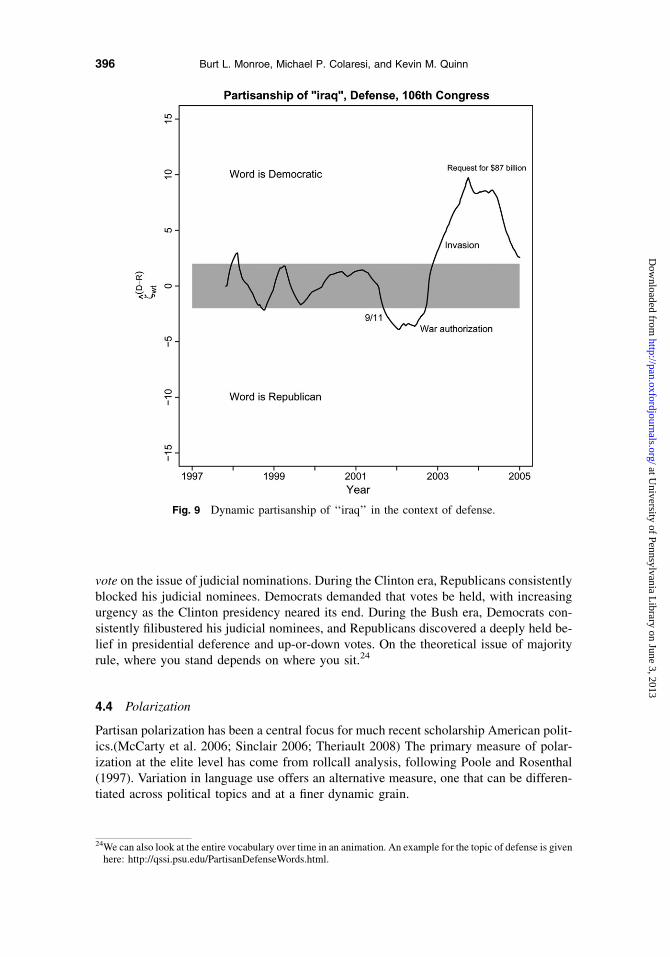
vote on the issue of judicial nominations. During the Clinton era, Republicans consistentlyblocked his judicial nominees. Democrats demanded that votes be held, with increasingurgency as the Clinton presidency neared its end. During the Bush era, Democrats con-sistently filibustered his judicial nominees, and Republicans discovered a deeply held be-lief in presidential deference and up-or-down votes. On the theoretical issue of majorityrule, where you stand depends on where you sit.24

4.4 Polarization

Partisan polarization has been a central focus for much recent scholarship American polit-ics.(McCarty et al. 2006; Sinclair 2006; Theriault 2008) The primary measure of polar-ization at the elite level has come from rollcall analysis, following Poole and Rosenthal(1997). Variation in language use offers an alternative measure, one that can be differen-tiated across political topics and at a finer dynamic grain.

Fig. 9 Dynamic partisanship of ‘‘iraq’’ in the context of defense.

24We can also look at the entire vocabulary over time in an animation. An example for the topic of defense is givenhere: http://qssi.psu.edu/PartisanDefenseWords.html.




Dow

nloaded from

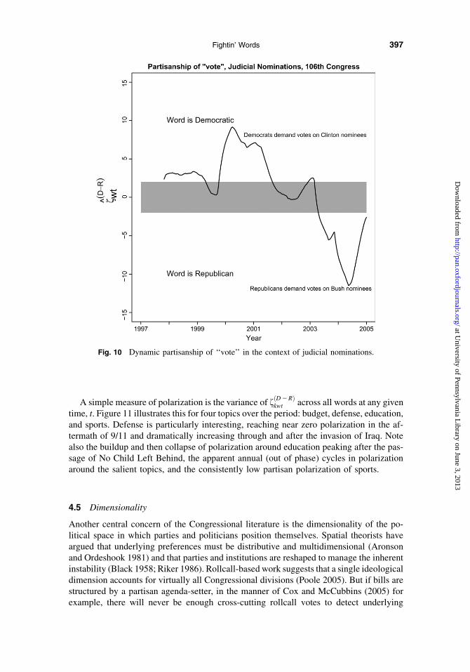
http://qssi.psu.edu/PartisanDefenseWords.html


A simple measure of polarization is the variance of fðD2RÞkwt across all words at any given

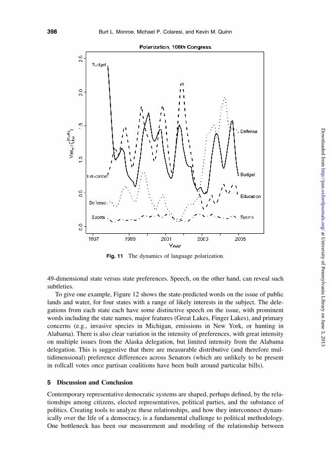
time, t. Figure 11 illustrates this for four topics over the period: budget, defense, education,and sports. Defense is particularly interesting, reaching near zero polarization in the af-termath of 9/11 and dramatically increasing through and after the invasion of Iraq. Notealso the buildup and then collapse of polarization around education peaking after the pas-sage of No Child Left Behind, the apparent annual (out of phase) cycles in polarizationaround the salient topics, and the consistently low partisan polarization of sports.

4.5 Dimensionality

Another central concern of the Congressional literature is the dimensionality of the po-litical space in which parties and politicians position themselves. Spatial theorists haveargued that underlying preferences must be distributive and multidimensional (Aronsonand Ordeshook 1981) and that parties and institutions are reshaped to manage the inherentinstability (Black 1958; Riker 1986). Rollcall-based work suggests that a single ideologicaldimension accounts for virtually all Congressional divisions (Poole 2005). But if bills arestructured by a partisan agenda-setter, in the manner of Cox and McCubbins (2005) forexample, there will never be enough cross-cutting rollcall votes to detect underlying

Fig. 10 Dynamic partisanship of ‘‘vote’’ in the context of judicial nominations.

397Fightin’ Words



Dow

nloaded from


49-dimensional state versus state preferences. Speech, on the other hand, can reveal suchsubtleties.

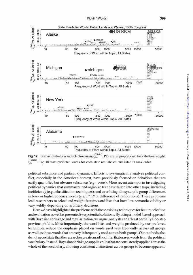
To give one example, Figure 12 shows the state-predicted words on the issue of publiclands and water, for four states with a range of likely interests in the subject. The dele-gations from each state each have some distinctive speech on the issue, with prominentwords including the state names, major features (Great Lakes, Finger Lakes), and primaryconcerns (e.g., invasive species in Michigan, emissions in New York, or hunting inAlabama). There is also clear variation in the intensity of preferences, with great intensityon multiple issues from the Alaska delegation, but limited intensity from the Alabamadelegation. This is suggestive that there are measurable distributive (and therefore mul-tidimensional) preference differences across Senators (which are unlikely to be presentin rollcall votes once partisan coalitions have been built around particular bills).

5 Discussion and Conclusion

Contemporary representative democratic systems are shaped, perhaps defined, by the rela-tionships among citizens, elected representatives, political parties, and the substance ofpolitics. Creating tools to analyze these relationships, and how they interconnect dynam-ically over the life of a democracy, is a fundamental challenge to political methodology.One bottleneck has been our measurement and modeling of the relationship between

Fig. 11 The dynamics of language polarization.




Dow

nloaded from


political substance and partisan dynamics. Efforts to systematically analyze political con-flict, especially in the American context, have previously focused on behaviors that areeasily quantified but obscure substance (e.g., votes). More recent attempts to investigatingpolitical dynamics that summarize and organize text have fallen into other traps, includinginefficiency (e.g., classification techniques), and overfitting idiosyncratic group differencesin low- or high-frequency words (e.g., tf.idf or difference of proportions). These problemslead researchers to select and weight feature/word lists that have low semantic validity orvary wildly depending on arbitrary decisions.

Herewehavehighlighted theproblems with these existing techniques for feature selectionand evaluation aswell as presented two potential solutions. By using a model-based approachwith Bayesian shrinkage and regularization, we argue, analysts can at least partially side-stepprevious pitfalls. Most importantly, the word lists and weights produced by our preferredtechniques reduce the emphasis placed on words used very frequently across all groupsas well as those words that are very infrequently used across both groups. Our methods alsodonotnecessitate that the researchercreateanadhocfilter that eraseswords fromthe politicalvocabulary. Instead,Bayesianshrinkagesuppliesrules thatareconsistentlyappliedacross thewhole of the vocabulary, allowing consistent distinctions across groups to become apparent.

Fig. 12 Feature evaluation and selection using fðStateÞkw . Plot size is proportional to evaluation weight,

fðStateÞkw . Top 10 state-predicted words for each state are labeled and listed in rank order.

399Fightin’ Words



Dow

nloaded from


We are, of course, ultimately concerned with whether these tools are useful for politicalanalysis. Our examples have shown that questions relating to issue framing, representation,polarization, and dimensionality can be explicitly explored with text data through our tech-niques. We expect that others working within these substantive fields will be able to carryout more detailed and extensive applications with these tools.

The next step is to further refine and craft methods that will be useful for unlocking theexciting potential of political texts. Our model-based regularization approach is one suchattempt. Although off-the-shelf algorithms and techniques have proven valuable, wemust look under the hood to know if we are validly measuring the concepts we care about.There is much that is theoretically and conceptually unique about the production oflanguage in politics, and there is a need for new methods to be developed and appliedaccordingly.

Funding

National Science Foundation (grant BCS 05-27513 and BCS 07-14688).

Appendix—Estimation of the Laplace Model

Maximization of the posterior densities in equations 28 and 29 is complicated by the dis-continuities in the partial derivatives that are introduced by the Laplace prior. We make useof a version of the algorithm of Shevade and Keerthi (2003) that has been modified to workwith a multinomial likelihood. Calculation of the relevant derivatives is tedious but notdifficult. In addition to moving from a Bernoulli to a multinomial likelihood, we also ex-tend the work of Shevade and Keerthi (2003) and Cawley and Talbot (2006) to allow anexponential prior for c.

Marginalizing over c with a Jeffreys Prior

Using results from Cawley and Talbot (2006), it is easy to show how the value of bðiÞk that

maximizes

pðbðiÞk jyðiÞk Þ}

Zp�yðiÞk jbðiÞ

k ÞpðbðiÞk jcÞpJðcÞdc ðA1Þ

can be calculated via a modified version of the iterative approach of Shevade and Keerthi(2003) in which, at each iteration, a working version, c, of c is defined to be:

c[W=XWw5 1

��bðiÞkw 2 bMLE

kw

��; ðA2Þ

and then the maximization over bðiÞkw is carried out conditional on c.

Marginalizing over c with an Exponential Prior

Using ideas similar to those described in the previous subsection to show how the value ofbðiÞk that maximizes




Dow

nloaded from


pðbðiÞk jyðiÞk Þ}

ZpðyðiÞk jbðiÞ

k ÞpðbðiÞk jcÞpEðcÞdc ðA3Þ

can be calculated via a modified version of the iterative approach of Shevade and Keerthi(2003) in which, at each iteration, a working version, c, of c is defined to be:

c[ðW1 1Þ

a1PWw5 1


kw

�� ðA4Þ

and then the maximization over bðiÞkw is carried out conditional on c.

Maximizing over c with an Exponential Prior

It is also possible to show that values of bðiÞk and c that maximizes


k ÞpðbðiÞk jcÞpEðcÞ ðA5Þ

can be calculated via a modified version of the iterative approach of Shevade and Keerthi(2003) in which, at each iteration, a local conditional maximizer for c is:

c[W

a1PWw5 1


kw

��; ðA6Þ

and then the maximization over bðiÞkw is carried out conditional on c.Note that when a 5 0, the results from this procedure are equivalent to those from the

setup where c is given a Jeffreys prior and then integrated out of the posterior.

References

Adams, Greg D. 1997. Abortion: Evidence of issue evolution. American Journal of Political Science 41(3):718–37.

Agresti, Alan. 2002. Categorical data analysis. 2nd ed. Hoboken, NJ: Wiley.

Aizawa, Akiko. 2003. An information-theoretic perspective of tf-idf measures. Information Processing and Man-

agement 39(1):45–65.

Aronson, Peter H., and Peter C. Ordeshook. 1981. Regulation, redistribution, and public choice. Public Choice

37(1):69–100.

Baumgartner, Frank R., Suzanna L. DeBoef, and Amber E. Boydstun. 2008. The decline of the death penalty and

the discovery of innocence. Cambridge: Cambridge University Press.

Black, Duncan. 1958. The theory of committees and elections. Cambridge: Cambridge University Press.

Breiman, Leo. 2001. Random forests. Machine Learning 45(1):5–32.

Carmines, Edward, and James Stimson. 1990. Issue evolution. New York: Princeton University Press.

Cawley, Gavin C., and Nicola L. C. Talbot. 2006. Gene selection in cancer classification using sparse logistic

regression with Bayesian regularization. Bioinformatics 22(19):2348–55.

Chong, Dennis, and James N. Druckman. 2007. Framing theory. Annual Review of Political Science 10:103–26.

Cox, Gary W., and Mathew D. McCubbins. 2005. Setting the agenda: Responsible party government in the US

House of Representatives. Cambridge: Cambridge University Press.

Diaz, Mercedes Mateo. 2005. Representing women? Female legislators in West European parliaments. Colches-

ter, UK: ECPR Press Monographs.

Diermeier, Daniel, Jean-Francois Godbout, Bei Yu, and Stefan Kaufmann. 2007. Language and ideology in

congress. Chicago, IL: Midwestern Political Science Association.

Emily, Senay, Eli H. Newberger, and Rob Waters. 2004. From boys to men. New York: Simon and Schuster.

Ericson, Matthew. 2008. The words they used. The New York Times, September 4, http://www.nytimes.com/

interactive/2008/09/04/us/politics/20080905_WORDS_GRAPHIC.html (accessed November 1, 2008).

Freund, Yoav, and Robert Schapire. 1997. A decision-theoretic generalization of on-line learning and an appli-

cation to boosting. Journal of Computer and System Sciences 55(1):119–39.

401Fightin’ Words



Dow

nloaded from




Gentzkow, Matthew, and Jesse M. Shapiro. 2006. What drives media slant? Evidence from U.S. daily newspapers.

University of ChicagoTechnical report.

Gilligan, Carol. 1993. In a different voice: Psychological theory and women’s development. Cambridge, MA:

Harvard University Press.

Hand, David J. 2006. Classifier technology and the illusion of progress. Statistical Science 21(1):1–14.

Hastie, Trevor, Robert Tibshirani, and Jerome Friedman. 2001. The elements of statistical learning. New York:

Springer.

Hiemstra, Djoerd. 2000. A probabilistic justification for using tfxidf term weighting in information retrieval.

International Journal on Digital Libraries 3:131–9.

Hillard, Dustin, Stephen Purpura, and John Wilkerson. 2007. Computer-assisted topic classification for mixed-

methods social science research. Journal of Information Technology and Politics 4(4):31–46.

Hopkins, Daniel, and Gary King. 2007. Extracting systematic social science meaning from text. Chicago, IL:

Midwestern Political Science Association.

Jurafsky, Daniel, and James H. Martin. 2000. Speech and language processing. Upper Saddle River, NJ:

Prentice Hall.

Kleinfeld, Judith, and Andrew Kleinfeld. 2004. Cowboy nation and American character. Society 41(3):43–50.

Krippendorff, Klaus. 2004. Content analysis: An introduction to its methodology. 2nd ed. New York: Sage.

Lakoff, George. 2004. Don’t think of an elephant! Know your values and frame the debate. White River Junction,

VT: Chelsea Green Publishing.

Laver, Michael, Kenneth Benoit, and John Garry. 2003. Extracting policy positions from political texts using

words as data. American Political Science Review 97:311–31.

Lowe, Will. 2008. Understanding Wordscores. Political Analysis doi:10.1093/pan/mpn004 (accessed October 4,

2008).

Manning, Christopher D., and Hinrich Schutze. 1999. Foundations of statistical natural language processing.

Cambridge, MA: MIT Press.

Manning, Christopher D., Prabhakar Raghavan, and Hinrich Schutze. 2008. An introduction to information

retrieval. Cambridge: Cambridge University Press.

Many Eyes (IBM). Tag Cloud Guide. http://manyeyes.alphaworks.ibm.com/manyeyes/page/Tag_Cloud.html

(accessed July 13, 2008).

McCaffrey, Dawn, and Jennifer Keys. 2008. Competitive framing processes in the abortion debate: Polarization-

vilification, frame saving, and frame debunking. Sociological Quarterly 41(1):41–61.

McCarty, Nolan, Keith T. Poole, and Howard Rosenthal. 2006. Polarized America: The dance of ideology and

unequal riches. Cambridge, MA: MIT Press.

Monroe, Burt L., Cheryl L. Monroe, Kevin M. Quinn, Dragomir Radev, Michael H. Crespin, Michael P. Colaresi,

Jacob Balazar, and Steven P. Abney. 2006. United States congressional speech corpus. State College, PA:

Pennsylvania State University.

Monroe, Burt L., and Ko Maeda. 2004. Rhetorical ideal point estimation: Mapping legislative speech. Society for

Political Methodology. Palo Alto: Stanford University.

Monroe, Burt L., Michael P. Colaresi, and Kevin M. Quinn. An Animated History of Senate Debate on Defense,

1997–2004. http://qssi.psu.edu/PartisanDefenseWords.html (accessed November 1, 2008).

Mucciaroni, Gary, and Paul J. Quirk. 2006. Deliberative choice: Debating public policy in congress. Chicago, IL:

University of Chicago Press.

Nunberg, Geoffrey. 2006. Talking right: How conservatives turned liberalism into a tax-raising, latte-drinking,

sushi-eating, volvo-driving, New York Times-Reading, Body-Piercing, Hollywood-Loving, Left-Wing Freak

Show. New York: Public Affairs.

Poole, Keith T. 2005. Spatial models of parliamentary voting. New York, Cambridge: Cambridge University Press.

Poole, Keith T., and Howard Rosenthal. 1997. Congress: A political-economic history of roll-call voting. Oxford:

Oxford University Press.

Porter, Martin F. 2001. The English (Porter2) stemming algorithm. http://snowball.tartarus.org/algorithms/

english/stemmer.html (accessed July 3, 2008).

Quinn, Kevin, Burt L. Monroe, Michael Colaresi, Michael Crespin, and Dragomir Radev. 2006. How to analyze

political attention with minimal assumptions and costs. Davis, CA: Society for Political Methodology.

Riker, William H. 1986. The art of political manipulation. New Haven, CT: Yale University Press.

Rokeach, Milton. 1973. The nature of human values. New York: The Free Press.

Sacerdote, Bruce, and Owen Zidar. 2008. Campaigning in poetry: Is there information conveyed in the candidates’

choice of words. Technical report, University of Dartmouth.

Schonhardt-Bailey, Cheryl. 2008. The congressional debate on partial-birth abortion: Constitutional gravitas and

moral passion. British Journal of Political Science 38(3):383–410.




Dow

nloaded from

http://manyeyes.alphaworks.ibm.com/manyeyes/page/Tag_Cloud.html

http://qssi.psu.edu/PartisanDefenseWords.html

http://snowball.tartarus.org/algorithms/english/stemmer.html

http://snowball.tartarus.org/algorithms/english/stemmer.html


Shevade, S. K., and S. S. Keerthi. 2003. A simple and efficient algorithm for gene selection using sparse logistic

regression. Bioinformatics 19(17):2246–53.

Sinclair, Barbara. 2006. Party wars: Polarization and the politics of national policy making. Norman, OK:

University of Oklahoma Press.

Slapin, Jonathan B., and Sven-Oliver Proksch. 2008. A scaling model for estimating time-series party positions

from texts. American Journal of Political Science 52(3):705–22.

Theriault, Sean M. 2008. Party polarization in congress. Cambridge: Cambridge University Press.

Vapnik, Vladimir. 2001. The nature of statistical learning theory. New York: Springer-Verlag.

Williams, Melissa S. 1998. Voice, trust and memory: Marginalized groups and the failings of liberal represen-

tation. Princeton, NJ: Princeton University Press.

Williams, Peter M. 1995. Bayesian regularization and pruning using a Laplace prior. Neural Computation

7(1):117–43.

Wordle. 2008. http://wordle.net (accessed July 13, 2008).

Yu, Bei, Stefan Kaufmann, and Daniel Diermeier. 2008. Classifying party affiliation from political speech. Journal

of Information Technology and Politics 5(1):33–48.

403Fightin’ Words



Dow

nloaded from

http://wordle.net


Documents

Fightin’ Words: Lexical Feature Selection and Evaluation for Identifying …languagelog.ldc.upenn.edu/myl/Monroe.pdf · Fightin’ Words: Lexical Feature Selection and ... Our proposed