-1-UNRESTRICTED / ILLIMITÉ

Field Implementation of a Transient Eddy

Current System for Carbon Steel Pipe

Thickness MeasurementsJeremy A. Buck, Colin Kramer, Jia Lei, and Brian A. Lepinejeremy.buck@cnl.ca 613-584-3311 ext. 42359

Canadian Nuclear Laboratories, Chalk River LaboratoriesInspection, Monitoring and Dynamics Branch

-2-UNRESTRICTED / ILLIMITÉ

• Tile hole storage arrays

• Inspection head and probe design

• Transient eddy current (TEC) testing theory

• Analysis methods and results

• Voltage-threshold analysis

• Power-law analysis

• TEC multi-frequency analysis

• Comparison to ultrasonic testing (UT) results

• Summary and conclusion

Outline

-3-UNRESTRICTED / ILLIMITÉ

• Engineered concrete structure for radioactive waste storage

• Multiple vertical tile holes

• Each tile hole has a carbon steel liner:

• 5 m long, and surrounded by concrete

• 250 mm inside diameter Schedule 40 pipe

• 9.3 mm nominal wall thickness

• Carbon steel is a common waste container material:

• Good structural properties

• Neutron absorber

Tile Hole Storage ArraysBackground

-4-UNRESTRICTED / ILLIMITÉ

Tile Hole Storage Arrays

• Inspection requirements:

• Determine overall condition of carbon steel pipes

• Report thickness to ±1 mm

• Flag if thickness <50% nominal

• Sample 10 tile holes from four separate arrays

• Challenges:

• Unknown pipe surface conditions

• Moderate liftoff (~13 mm)

• Ferromagnetic material

• No prior inspection data

Inspection Requirements and Challenges

-5-UNRESTRICTED / ILLIMITÉ

Inspection HeadDesign Approach

TEC Sensors

UT Transducers

• Inspection head combining TEC and UT probes

• Complimentary techniques

• 8 UT transducers

• 8 TEC coil pairs

• Sensors evenly spaced in 45° intervals

• Couplant not required for TEC inspection

-6-UNRESTRICTED / ILLIMITÉ

Inspection Head

• Two TEC sensor designs:

• “Reflection” coil pairs (T1R1, T2R3, T3R5, T4R7)

• “Transmit/Receive” coil pairs (R2, R4, R6, R8)

• Sensor designs alternated around the probe

• Two scans of each tile hole were performed, rotating the inspection head 45°, for full coverage with both probe types

• TEC measurements collected every 100 mm translating down the pipe

TEC SensorsT1 R2

R1

-7-UNRESTRICTED / ILLIMITÉ

Transient Eddy Current (TEC) Testing

• Eddy currents generated via Faraday’s Law:

휀 = −𝑁𝑑𝜑

𝑑𝑡• Broadband voltage pulse used to induce eddy currents

• Eddy currents decay following a diffusion process

• TEC testing much less susceptible to skin effects

Theory

0

2

4

6

8

10

12

0 20 40 60 80 100

Vo

ltag

e (V

)

Time (ms)

0

0.1

0.2

0.3

0.4

0.5

0.6

0.7

0 20 40 60 80 100

Vo

ltag

e (V

)

Time (ms)

-8-UNRESTRICTED / ILLIMITÉ

Analysis Methods

• Signal-to-noise ratio of T/R data hindered analysis, so reflection data was exclusively examined.

• Three analysis techniques were applied to the TEC data:

• Voltage-threshold analysis

• Power-law analysis

• TEC multi-frequency analysis

Overview

-9-UNRESTRICTED / ILLIMITÉ

Voltage-Threshold AnalysisMethod

-10-UNRESTRICTED / ILLIMITÉ

Voltage-Threshold

• Channels calibrated independently for each scan to compensate for thickness variations around the calibration pipe and slight differences in probe response

• A linear interpolation was used to estimate unknown thickness

%𝑊𝑇 = 100 −𝑊𝑇𝑁𝑂𝑀 −𝑊𝑇𝐼𝐷𝐶𝑁𝑂𝑀 − 𝐶𝐼𝐷

∗ 𝐶𝑁𝑂𝑀 − 𝐶𝑀𝑒𝑎𝑠𝑢𝑟𝑒𝑚𝑒𝑛𝑡

• Assumed thickness and voltage-threshold relationship was linear

Calibration

-11-UNRESTRICTED / ILLIMITÉ

Voltage-ThresholdInspectionWare

-12-UNRESTRICTED / ILLIMITÉ

Voltage-ThresholdResults

0°

90°

180°

270°

6

7

8

9

10

11

12

4800 4400 4000 3600 3200 2800 2400 2000 1600 1200 800 400 0

Angular Position

Thic

knes

s [m

m]

Axial Position [mm]

-13-UNRESTRICTED / ILLIMITÉ

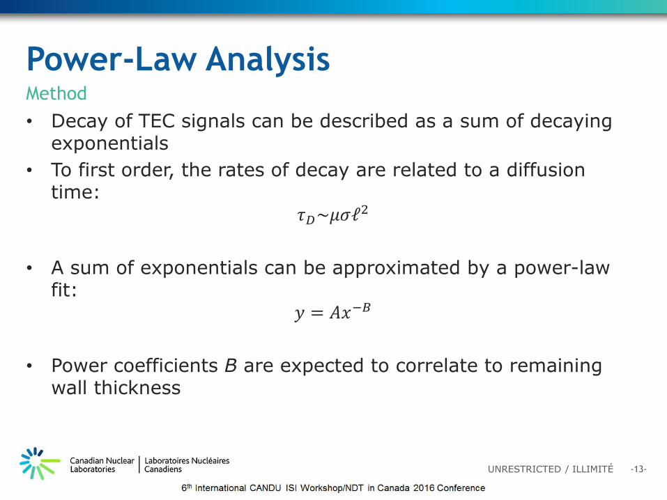
Power-Law Analysis

• Decay of TEC signals can be described as a sum of decaying exponentials

• To first order, the rates of decay are related to a diffusion time:

𝜏𝐷~𝜇𝜎𝓁2

• A sum of exponentials can be approximated by a power-law fit:

𝑦 = 𝐴𝑥−𝐵

• Power coefficients B are expected to correlate to remaining wall thickness

Method

-14-UNRESTRICTED / ILLIMITÉ

Power-Law Analysis

• Each channel calibrated independently

• Data were windowed from 3 to 30 ms before power fit after window optimization based on lab data

• Analysis was performed post-acquisition using MATLAB

Calibration

y = 574.88x-3.49

y = 580.41x-3.498

y = 380.51x-3.434

y = 354.26x-3.3860.001

0.01

0.1

1

10

6

Log(

Vo

ltag

e) [

V]

Log(Time) [ms]

T1R1

T2R3

T3R5

T4R7

-15-UNRESTRICTED / ILLIMITÉ

Power-Law AnalysisResults

0°

90°

180°

270°

6

7

8

9

10

11

12

4800 4400 4000 3600 3200 2800 2400 2000 1600 1200 800 400 0

Angular Position

Thic

knes

s [m

m]

Axial Position [mm]

-16-UNRESTRICTED / ILLIMITÉ

TEC Multi-Frequency Analysis*

• Requires a Fourier Transform be applied to the data

• Fourier components normalized through complex division of reference point components at each frequency

• Liftoff Fourier components normalized and subtracted from measurement components

• Analytic approximations of

Skin Depth: 𝛿 = 50𝜌

𝑓𝜇

Amplitude: A = s(δ/2)(1+p)(e−2x/δ−e−2w/δ)

Phase: φ = φ0 + φl + 1 + 2/δ(we−2w/δ − xe−2x/δ)/(e−2w/δ − e−2x/δ)*presented in greater detail by Dag Horn at this conference.

Method

-17-UNRESTRICTED / ILLIMITÉ

TEC Multi-Frequency AnalysisResults

0°

90°

180°

270°

6

7

8

9

10

11

12

4800 4400 4000 3600 3200 2800 2400 2000 1600 1200 800 400 0

Angular Position

Thic

knes

s [m

m]

Axial Position [mm]

-18-UNRESTRICTED / ILLIMITÉ

Ultrasonic TestingResults

0°

90°

180°

270°

6

7

8

9

10

11

12

4800 4400 4000 3600 3200 2800 2400 2000 1600 1200 800 400 0

Angular Position

Thic

knes

s [m

m]

Axial Position [mm]

-19-UNRESTRICTED / ILLIMITÉ

Comparison of Results

• UT thickness estimates accepted as accurate measurements

• TEC analysis-method means compared to UT means

• On average, TEC multi-frequency analysis outperformed the other two methods

Tile Hole

UT Voltage Threshold Power Law TEC MFAMean Mean SD % diff Mean SD % diff Mean SD % diff

1 9.3 8.2 0.5 12 8.8 0.3 5 9.1 0.4 2

2 9.2 7.4 0.9 19 8.8 0.4 4 9.5 0.4 -33 9.8 8.2 0.6 16 9.2 0.4 6 9.6 0.4 24 9.6 7.6 0.7 20 9.4 0.4 3 9.4 0.3 25 9.6 8.7 1.1 10 9.2 0.3 5 9.3 0.4 3

6 9.5 8.5 1.1 11 8.7 0.3 8 9.3 0.4 27 9.3 7.8 0.9 16 9.5 0.2 -2 9.7 0.3 -5

8 9.3 7.7 0.7 17 9.5 0.4 -2 9.7 0.3 -4

9 9.6 8.4 0.5 13 9.2 0.3 5 9.6 0.4 0

10 9.4 7.4 0.7 21 9.3 0.3 1 9.6 0.2 -2

Average 9.5 8.0 0.8 15 9.2 0.3 3 9.5 0.4 0

-20-UNRESTRICTED / ILLIMITÉ

Conclusions• Inspection requirements met by TEC and UT:

• No regions of wall thinning beyond nominal tolerance reported

• Good overall agreement with UT measurements qualitatively and quantitatively

• TEC method sensitive enough to identify pilger manufacturing process in ferromagnetic pipes (~0.5 mm amplitude ripples)

• Liquid couplant not required for TEC inspection

• Voltage-threshold most sensitive to low-voltage noise

• Power-law and TEC multi-frequency analysis methods are more closely related to electromagnetic phenomena, and produced more accurate results

• Electromagnetic inspection of ferromagnetic pipe has been successfully demonstrated

-21-UNRESTRICTED / ILLIMITÉ

Questions