NUREG/CR-6984 PNNL-14374

Field Evaluation of Low-Frequency SAFT-UT on Cast Stainless Steel and Dissimilar Metal Weld Components

Office of Nuclear Regulatory Research

Abstract

This report documents work performed at the Pacific Northwest National Laboratory (PNNL) in Richland, Washington, and at the Electric Power Research Institute’s (EPRI) Nondestructive Examination (NDE) Center in Charlotte, North Carolina, on evaluating a low-frequency ultrasonic inspection technique used for examination of cast austenitic stainless steel (CASS) and dissimilar metal (DMW) reactor piping components. It should be noted that this work predates efforts recently published in two reports: NUREG/CR-6933, “Assessment of Crack Detection in Heavy-Walled Cast Stainless Steel Piping Welds Using Advanced Low-Frequency Ultrasonic Methods,” published in March 2007 (Anderson et al. 2007), and NUREG/CR-6929, “Assessment of Eddy Current Testing for the Detection of Cracks in Cast Stainless Steel Reactor Piping Components,” published in February 2007 (Diaz et al. 2007). The results of the earlier work are being published because it was conducted semi-blind and will be a valuable source of information relative to performance demonstration assessments. In addition, there were some examinations of DMWs, and the number of studies published to date providing DMW examination results are limited. The early work demonstrated the potential for using low-frequency ultrasound coupled with synthetic aperture focusing technique (SAFT) signal processing to detect cracking in coarse-grained stainless steels. The follow-on efforts are detailed in NUREG/CR-6929 and NUREG/CR-6933. It should be noted that the inspection techniques have greatly improved since the initial work; in particular, the use of low-frequency phased arrays which permits faster inspections, more flexible and precise scans, and better detectability. The technique discussed in this report uses a zone-focused, multi-incident angle, low-frequency (250–450 kHz) inspection protocol coupled with the synthetic aperture focusing technique (SAFT). The primary focus of this work is to provide information to the United States Nuclear Regulatory Commission on the utility, effectiveness and reliability of ultrasonic testing (UT) inspection techniques as related to the inservice ultrasonic inspection of coarse grained primary piping components in pressurized water reactors (PWRs). Experiments were conducted in order to assess the low-frequency (350 kHz) ultrasonic inspection technique for coarse-grained stainless steel components. Software was modified and experiments were performed for applying a noise reduction algorithm to the pre- and post-SAFT processed data sets. PNNL staff traveled to the EPRI NDE Center to examine samples from the inventory of Westinghouse Owner’s Group (WOG) CASS and DMW sections. The results reported here do not represent data from a statistically large number of field-representative CASS samples. Approximately 20 CASS specimens (PNNL and EPRI specimens) were examined using this examination protocol. Results from this field test clearly show that the low-frequency/SAFT inspection technique is capable of providing quality detection and localization data, and accurate length sizing information.

iii

NUREG/CR-6984 PNNL-14374

Field Evaluation of Low-Frequency SAFT-UT on Cast Stainless Steel and Dissimilar Metal Weld Components Manuscript Completed: August 2008 Date Published: November 2008 Prepared by A.A. Diaz, R.V. Harris, S.R. Doctor

Pacific Northwest National Laboratory P.O. Box 999 Richland, WA 99352 D.A. Jackson and W.E. Norris, NRC Project Managers

NRC Job Code N6398 Office of Nuclear Regulatory Research

FOREWORD

The low cost and relative corrosion-resistance of cast austenitic stainless steel (CASS) have resulted in its extensive use in the primary pressure boundary of pressurized-water reactors (PWRs). This is significant because Section XI of the Boiler and Pressure Vessel Code promulgated by the American Society of Mechanical Engineers (ASME) requires periodic inservice inspection of welds in the primary pressure boundary, including those that are fabricated using CASS. In most applications, ultrasonic testing (UT) techniques can reliably detect and accurately size flaws that may occur during service. However, this is not the case for CASS because its coarse-grained non-homogeneous, anisotropic microstructure makes components constructed with CASS difficult to inspect. Anisotropic means that the material properties are direction dependant. Because of the anisotropic nature of CASS, the reflection of the ultrasound wave is highly dependent on any given point in the material. This is because the large and dissimilar grain sizes of CASS strongly affect the propagation of ultrasound waves by causing severe attenuation (loss of energy or magnitude), changes in velocity, and scattering of ultrasonic waves. As a result, it can be difficult to distinguish scatter from flaw-induced signal patterns. In addition, redirection of the ultrasonic waves may result in incomplete examination. Given these issues, the U.S. Nuclear Regulatory Commission (NRC), Office of Nuclear Regulatory Research (RES), sponsored research at the Pacific Northwest National Laboratory (PNNL) to assess the reliability and effectiveness of various nondestructive examination (NDE) techniques for inspecting coarse-grained materials like CASS. Two recently published reports provide results from this work. NUREG/CR-6933, “Assessment of Crack Detection in Heavy-Walled Cast Stainless Steel Piping Welds Using Advanced Low-Frequency Ultrasonic Methods,” published in March 2007, discusses the effectiveness and reliability of advanced low-frequency UT to penetrate thick-walled sections of CASS primary piping to detect inside surface-breaking cracks from the outside surface. NUREG/CR-6929, “Assessment of Eddy Current Testing for the Detection of Cracks in Cast Stainless Steel Reactor Piping Components,” published in February 2007, discusses the results of a study of advanced eddy-current probe configurations sensitive to near-surface flaws in both axial and circumferential orientations. To augment those studies, this report documents earlier research performed by PNNL at their laboratory in Richland, Washington, and at the Electric Power Research Institute (EPRI) Nondestructive Examination Center (NDE) in Charlotte, North Carolina. The research was conducted to evaluate a zone-focused low-frequency (250–450 kHz) ultrasonic inspection protocol coupled with the synthetic aperture focusing technique (SAFT) for use in examining reactor piping components that are fabricated using CASS and dissimilar metal welds (DMWs), which are located in safety-related systems of nuclear power plants. Before beginning that research, PNNL, EPRI, and the NRC mutually agreed to interact throughout the study, sharing ultrasonic data and information in order to conduct a more effective and thorough evaluation of the inspection problem. The purpose of the experiments at PNNL was to assess the low-frequency ultrasonic inspection technique for CASS. The EPRI NDE exercise was to evaluate the effectiveness of the low-frequency/SAFT inspection protocol under more realistic, field-representative conditions (using piping specimens furnished by the Westinghouse Owner’s Group) and further refine crack identification and sizing criteria. This study demonstrated the potential for using low-frequency ultrasound, coupled with SAFT signal processing, to detect cracking in coarse-grained stainless steels, and established the groundwork for the efforts detailed in NUREG/CR-6929 and NUREG/CR-6933. As a result, inspection techniques (particularly the use of low-frequency phased arrays) have greatly improved since the initial work.

v

vi

In publishing this report, the NRC’s purpose is to make the research results publicly available because the investigation was semi-blind and its results will be a valuable source of information for future performance demonstration assessments. Moreover, this report addresses examinations of DMWs, for which only limited data have previously been published. In addition, the NRC has presented the results of the PNNL and EPRI research to the cognizant ASME committees as technical justification for initiating the necessary work to improve the reliability and effectiveness of the inspection of these materials.

Contents

Abstract .............................................................................................................................................. iii Foreword............................................................................................................................................ v Executive Summary ........................................................................................................................... ix Acknowledgments.............................................................................................................................. xiii Abbreviations and Acronyms ............................................................................................................ xv 1 Introduction................................................................................................................................ 1.1

1.1 Experimental Approach..................................................................................................... 1.1

1.2 Examination Specimens .................................................................................................... 1.3

2 Low-Frequency Ultrasonic Data Acquisition ............................................................................ 2.1

2.1 Low-Frequency, Variable-Angle Search Unit ................................................................... 2.3

3 Signal Processing ....................................................................................................................... 3.1

3.1 Examination Procedures .................................................................................................... 3.2

3.2 Crack Identification and Sizing Criteria ............................................................................ 3.4

3.3 Examination Results .......................................................................................................... 3.6

4 Conclusions................................................................................................................................ 4.1 5 References .................................................................................................................................. 5.1 Appendix A – Velocity and Specimen Information Templates ......................................................... A.1 Appendix B – Discussion of Specimens ............................................................................................ B.1 Appendix C – Step-by-Step Various Stages of Analysis Using the

SAFT-Processed Ultrasonic Images ........................................................................... C.1

vii

viii

Figures

1.1 Side View of Typical WOG CASS Specimen......................................................................... 1.5

1.2 Underside View of Typical WOG CASS Specimen ............................................................... 1.5

1.3 Side View of Typical WOG DMW Specimen ........................................................................ 1.7

1.4 Underside View of Specimen “H”, 100% Through-Wall Crack, 35.56-cm Long .................. 1.8

2.1 Schematic of Low-Frequency Ultrasonic Data Acquisition System ....................................... 2.2

2.2 View of Instrumentation and Scanner Set-up in the EPRI High Bay Facility......................... 2.3

2.3 Low-Frequency, Variable-Angle Search Unit......................................................................... 2.4

3.1 Data Analysis Being Conducted by Ms. Deborah Jackson (NRC) and Dr. Robert Harris (PNNL) ................................................................................................ 3.1

3.2 Illustration Defining the “Area of Interest” for Crack Definition ........................................... 3.4

3.3 Graphical Summary of Inspection Results .............................................................................. 3.13

4.1 True Surface Length of WOG Specimen Flaws versus Ultrasonically Estimated Lengths............................................................................................ 4.2

4.2 Circumferential Flaw Center Position on Surface ................................................................... 4.2

4.3 Overlapped Length as a Fraction of Total Length for Specimens A through H...................... 4.3

4.4 Overlapped Length of Flaws versus True Length of Flaws .................................................... 4.3

4.5 Overlapped Length of Flaws versus Total Length of Flaws.................................................... 4.4

Tables

3.1 Actual Flaw Dimensions for Specimens Examined at EPRI................................................... 3.7

3.2 Actual Flaw Dimensions versus Measured Flaw Dimensions ................................................ 3.8

Executive Summary

This report documents work performed at the Pacific Northwest National Laboratory (PNNL) in Richland, Washington, and at the Electric Power Research Institute’s (EPRI) Nondestructive Examination (NDE) Center in Charlotte, North Carolina, on evaluating a low-frequency ultrasonic inspection technique used for examination of cast austenitic stainless steel (CASS) and dissimilar metal weld (DMW) reactor piping components. It should be noted that this work predates efforts recently published in two reports: NUREG/CR-6933, “Assessment of Crack Detection in Heavy-Walled Cast Stainless Steel Piping Welds Using Advanced Low-Frequency Ultrasonic Methods,” published in March 2007, and NUREG/CR-6929, “Assessment of Eddy Current Testing for the Detection of Cracks in Cast Stainless Steel Reactor Piping Components,” published in February 2007. The results of the earlier work are being published because it was conducted semi-blind and will be a valuable source of information relative to performance demonstration assessments. In addition, there were some examinations of DMWs, and the number of studies published to date providing DMW examination results are limited. The early work demonstrated the potential for using low-frequency ultrasound coupled with synthetic aperture focusing technique (SAFT) signal processing to detect cracking in coarse-grained stainless steels. The follow-on efforts are detailed in NUREG/CR-6929 and NUREG/CR-6933. It should be noted that the inspection techniques have greatly improved since the initial work; in particular, the use of low-frequency phased arrays. The technique uses a zone-focused low-frequency (250–450 kHz) inspection protocol coupled with the synthetic aperture focusing technique (SAFT). The primary focus of this work is to provide information to the United States Nuclear Regulatory Commission on the utility, effectiveness and reliability of ultrasonic testing (UT) inspection techniques as related to the inservice ultrasonic inspection of primary piping components in pressurized water reactors (PWRs). PNNL staff traveled to the EPRI NDE Center in Charlotte, North Carolina, to conduct a performance evaluation of the low-frequency/SAFT inspection method on coarse-grained, CASS, and DMW piping components. The EPRI NDE Center provided technical support and access to the Westinghouse Owner’s Group (WOG) CASS and DMW piping specimens. Experiments were conducted in order to assess the low-frequency ultrasonic inspection technique for coarse-grained stainless steel components. Enhancements were made to the software and experiments were performed for applying a noise reduction algorithm to the pre- and post-SAFT processed data sets. Prior to the start of the evaluation, staff from EPRI, PNNL and the U.S. Nuclear Regulatory Commission (NRC) agreed to mutually interact throughout the exercise, sharing ultrasonic data and pertinent information associated with the inspection problem in order to more effectively conduct a thorough evaluation of the low-frequency inspection technique coupled with SAFT. The examination protocol is based upon the premise that there exist sufficient differences between the characteristics of coherently scattered ultrasonic energy from grain boundaries and geometrical reflectors and the scattered ultrasonic energy from surface-breaking thermal and mechanical fatigue cracks in coarse grained steels. PNNL’s empirical approach relies on the notion that propagational effects due to acoustic impedance variations at the grain boundaries can be minimized by using lower frequencies (longer wavelengths), and the degree of coherent energy scattered from these grain boundaries should be

ix

inconsistent as a function of frequency, insonification angle, scan direction, and the amplitude of returning signals. The low-frequency/SAFT approach is directed toward detecting the corner-trap response from the surface-breaking crack as a function of time, spatial position, and amplitude. If the frequency is low enough, the examination is less sensitive to the effects of the microstructure and the probability of detection increases for surface-breaking cracks. The tradeoff is resolution. However, with the addition of SAFT signal processing, the examination can be performed at low frequencies while maintaining the capability to detect inside surface-breaking thermal and mechanical fatigue cracks greater than approximately 35%( )a through-wall depth in typical CASS and DMW piping components, provided that access to the outside surface was sufficient for adequate transducer placement and coupling. Further, cracks on the order of 15–35% through-wall can be periodically detected using a 500-kHz phased array method. Therefore, by utilizing multiple examination frequencies and incident angles, and inspecting from both sides of the weld, the low-frequency/SAFT technique invokes a composite approach for detection, localization and sizing of cracks in CASS and DMW material. The examination process is further enhanced by the addition of a low-frequency, variable-angle, high-bandwidth search unit that enables the inspector to compensate for acoustic velocity variations due to the microstructure by selecting the optimal incident angle in the material under test. The high bandwidth allows the inspector to utilize a wide range of examination frequencies centered around 350 kHz. The zone-focal characteristics of the dual element search unit provide optimal insonification of the inner surface (ID) over a specified range of incident angles. The purpose of conducting the exercise at the EPRI NDE Center was to evaluate the performance of the low-frequency/SAFT inspection approach under more realistic, field representative conditions in order to determine the effectiveness of this examination protocol and further refine the crack identification and sizing criteria. The work conducted at PNNL and during the EPRI field exercise demonstrates the potential for useful crack detection in CASS and DMW materials using low-frequency ultrasound. Specifically, an ultrasonic inspection technique coupled with SAFT signal processing, utilizing the full complement of examination angles (0°, 30°, 45°, and 60° from both sides of the weld) in the longitudinal wave mode, in a pitch-catch configuration at low frequencies has demonstrated a good probability of detection for fatigue cracking in coarse-grained stainless steels. Utilization of the SAFT for signal processing coupled with the low-frequency UT technique in a field test at the EPRI NDE Center provided positive results with respect to detection, localization and length sizing. The experimental results indicate that this low-frequency/SAFT technique is capable of consistently detecting and sizing circumferentially oriented thermal and mechanical fatigue cracks on the order of 35% deep and greater and 3.81 cm (1.5 in.) in extent and longer, in CASS and DMW components, as well as fabricated 10% deep circumferential notches, 25% deep circumferential sawcuts, end-of-block corner traps, and 1.59 mm (1/16 in.) diameter circumferential side drilled holes.

(a) Future work and probe enhancements have resulted in significant improvements for detecting smaller

flaws.

x

These results do not represent data from a statistically large number of field-representative CASS samples. Approximately 20 CASS specimens (PNNL and EPRI specimens) were examined using this inspection protocol. Results from this field test clearly show that the low-frequency/SAFT inspection technique is capable of providing quality detection and localization data, and accurate length sizing information.

xi

xii

Acknowledgments

The work reported here was conducted under JCN W6275 and written under JCN Y6604, with technical guidance provided by Ms. Deborah Jackson, and Mr. Wallace Norris, the NRC Project Monitors. Ms. Jackson’s participation in the field exercise at EPRI is also very much appreciated. In addition, we thank Mr. Harold Gray (NRC Region 1) for his participation and technical support during the EPRI field exercise. The majority of the work reported here was conducted at the EPRI NDE Center in Charlotte, North Carolina, and PNNL staff appreciate the opportunity to work with the following EPRI staff members who demonstrated their hospitality and technical support throughout the two-week visit. We thank Mr. Stan Walker, Mr. Steve Kenefick, Mr. Jeff Landrum, Mr. F. Larry Becker, and Dr. Doug MacDonald. The re-engineered ultrasonic search unit was developed and manufactured by Mr. Gary Langlois of Sigma Transducers Inc., Kennewick, Washington. At PNNL, the authors wish to thank Mr. Robert Bowey, Mr. Doug Riechers, and Mr. George Schuster for their technical support, advice and assistance on this project.

xiii

xiv

Abbreviations and Acronyms

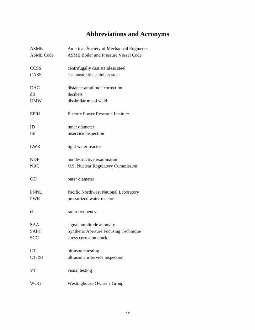
ASME American Society of Mechanical Engineers ASME Code ASME Boiler and Pressure Vessel Code CCSS centrifugally cast stainless steel CASS cast austenitic stainless steel DAC distance-amplitude correction dB decibels DMW dissimilar metal weld EPRI Electric Power Research Institute ID inner diameter ISI inservice inspection LWR light water reactor NDE nondestructive examination NRC U.S. Nuclear Regulatory Commission OD outer diameter PNNL Pacific Northwest National Laboratory PWR pressurized water reactor rf radio frequency SAA signal amplitude anomaly SAFT Synthetic Aperture Focusing Technique SCC stress corrosion crack UT ultrasonic testing UT/ISI ultrasonic inservice inspection VT visual testing WOG Westinghouse Owner’s Group

xv

xvi

1 Introduction

The low cost and relative corrosion-resistance of cast austenitic stainless steel (CASS) have resulted in extensive use of this material in the primary pressure boundary of light water reactors (LWRs). These materials are subjected to a volumetric examination based on the requirements of Section XI of the American Society of Mechanical Engineers Boiler and Pressure Vessel Code (ASME Code). The volumetric examination may be either radiographic or ultrasonic. For inservice examinations, background radiation and access limitations generally prevent the use of radiography. Hence, cast austenitic welds in primary piping loops of LWRs are subject to ultrasonic inservice inspection. The purpose of ultrasonic inservice inspection (UT/ISI) of nuclear reactor piping and pressure vessels is the reliable detection and accurate sizing of material defects. Before defects can be sized, they must first be detected. This is typically done by analyzing ultrasonic echo waveforms from material defects. Due to the coarse microstructure of CASS material, many inspection problems exist and are common to structures such as cladded pipe, inner-surface cladding of pressure vessels, statically cast elbows, statically cast pump bowls, centrifugally cast stainless steel (CCSS) piping, dissimilar metal welds (DMW), and weld-overlay-repaired pipe joints. Far-side weld inspection of stainless steels is an inspection technique included in the work scope since the ultrasonic field must pass through weld material. Because CCSS piping is used in the primary reactor coolant loop piping of 27 pressurized water reactors (PWRs) manufactured by the Westinghouse Electric Corporation, there exists a need to develop effective and reliable inspection techniques for these components. CCSS inspection procedures continue to perform unsatisfactorily due to the coarse microstructure that characterizes these materials. The major microstructural classifications are columnar, equiaxed, and mixed columnar-equiaxed microstructure of which the majority of field material is believed to be the latter. CCSS is an anisotropic and nonhomogeneous material. The manufacturing process can result in the formation of a long columnar grain structure, (approximately normal to the surface) with grain growth oriented along the direction of heat dissipation, often several centimeters in length. During the solidification of the material, columnar equiaxed (randomly speckled microstructure), or a mixed structure can result depending on chemical content and control of the cooling process (NUREG/CR-6594; Diaz et al. 1998). The large size of the anisotropic grains, relative to the acoustic pulse wavelength, strongly affects the propagation of ultrasound by causing severe attenuation, changes in velocity, and scattering of ultrasonic energy. Refraction and reflection of the sound beam occur at the grain boundaries resulting in defects being incorrectly reported, specific volumes of material not being examined, or both. When coherent reflection and scattering of the sound beam occur at the grain boundaries, ultrasonic indications occur which are difficult to distinguish from signals originating from flaws. When inspecting pipe sections, where the signal-to-noise ratio is relatively low, ultrasonic examinations can be confusing, unpredictable and unreliable. 1.1 Experimental Approach

Staff from the Pacific Northwest National Laboratory (PNNL) traveled to the Electric Power Research Institute’s (EPRI) NDE Center in Charlotte, North Carolina, to conduct a performance evaluation of the low-frequency/synthetic aperture focusing technique (SAFT) inspection method on coarse grained,

1.1

CASS, and DMW piping components. The EPRI NDE Center hosted the inspection team from PNNL, providing technical support and an area located in the NDE Center’s high-bay facility to perform ultrasonic examinations on Westinghouse Owner’s Group (WOG) cast austenitic stainless steel and dissimilar metal weld piping specimens. Prior to the start of the evaluation, staff from EPRI, PNNL and the U.S. Regulatory Commission (NRC) agreed to mutually interact throughout the exercise sharing ultrasonic data and pertinent information associated with the inspection problem in order to more effectively conduct a thorough evaluation of the low-frequency inspection technique coupled with SAFT. Extensive laboratory work was performed at PNNL prior to the exercise. PNNL staff examined aluminum and CASS calibration blocks as well as numerous CASS pipe-to-pipe sections and one DMW calibration block. The calibration blocks, CASS pipe-to-pipe sections and DMW calibration block, were used to evaluate various performance characteristics associated with the ultrasonic inspection system, including detection, resolution and sizing limitations, inspection parameters, and imaging characteristics associated with various SAFT signal processing parameters. Although the specimens examined at PNNL exhibited all of the necessary reflector types, including corner-trap geometries, side drilled holes, notches, weldment geometries and thermal/mechanical fatigue cracks, these specimens did not exhibit field representative conditions associated with inner-diameter (ID) and outer-diameter (OD) surface contours, wall thickness, component geometry, coarseness and grain orientation of the various microstructures, weldment geometry and counterbore, and access limitations associated with these conditions. Previous work, coupled with prior participation in CASS round robins, provided a foundation for development of a framework for crack identification and sizing criteria using the low-frequency/SAFT approach. Therefore, the purpose of conducting the exercise at the EPRI NDE Center was to evaluate the performance of the low-frequency/SAFT inspection approach under more field representative conditions in order to determine the effectiveness of this examination protocol and further refine the crack identification and sizing criteria. PNNL staff used EPRI CASS and DMW calibration blocks and two WOG CASS training specimens with known reflector and crack information to refine the low-frequency/SAFT crack identification and sizing criteria. The focus of the examination was directed toward crack detection localization, and length sizing but not depth sizing. Initially, the PNNL team had determined that the examination should focus on the specimens exhibiting cracks of categorically larger dimensions (i.e., cracks of 5.08 cm (2.0 in.) in length and longer, and depths of 35–40% through-wall and deeper). This was based upon extensive fracture mechanics work conducted at PNNL that guided inspections to focus on cracking that potentially challenged the structural integrity of the components. EPRI provided the PNNL inspection team with those WOG specimens that contained the largest flaw depths and extent that were present in the EPRI inventory, however, most of the specimens provided for the evaluation contained cracking that bordered on the lower limits of detection of the low-frequency/SAFT inspection system, between 25% and 35% through-wall depth and between 3.81 cm (1.5 in.) and 8.89 cm (3.5 in.) in length. The examination protocol is based upon the premise that sufficient differences exist between the characteristics of coherently scattered ultrasonic energy from grain boundaries and geometrical reflectors and the scattered ultrasonic energy from surface-breaking thermal and mechanical fatigue cracks in coarse grained steels. PNNL’s empirical approach relies on the notion that acoustic impedance variations at the grain boundaries can be minimized by using lower frequencies (longer wavelengths), and the degree of coherent energy scattered from these grain boundaries should be inconsistent as a function of frequency, insonification angle, scan direction, and the amplitude of returning signals. The low-frequency/SAFT

1.2

approach is directed toward detecting the corner-trap response from the surface-breaking crack as a function of time, spatial position, and amplitude. If the frequency is low enough, the examination is less sensitive to the effects of the microstructure and the probability of detection increases for surface-breaking cracks. The tradeoff is resolution. However, with the addition of SAFT signal processing, the examination can be performed at low frequencies while maintaining the capability to detect cracks approximately 35% deep or greater in typical CASS and DMW piping components. Therefore, by utilizing multiple examination frequencies and incident angles, and inspecting from both sides of a weld, the low-frequency/SAFT technique invokes a composite approach for detection, localization and sizing of cracks in CASS and DMW material. The examination process is further enhanced by the addition of a low-frequency, variable angle, high bandwidth search unit which enables the inspector to compensate for acoustic velocity variations due to the microstructure by selecting the optimal incident angle in the material under test. The high bandwidth allows the inspector to utilize a wide range of examination frequencies centered around 350 kHz. The zone-focal characteristics of the dual element search unit provide optimal insonification of the ID over a range of incident angles. 1.2 Examination Specimens

Twelve specimens (sectioned components) were examined during the evaluation exercise. One calibration block that was shipped from PNNL, two EPRI NDE Center CASS calibration blocks, one EPRI NDE Center DMW calibration block, one EPRI NDE Center pipe section with a 100% through-wall mechanical fatigue crack, six WOG CASS sections, and one WOG DMW section comprise the list of specimens examined. All WOG specimens described in this study will be identified only by a capital letter (e.g., WOG Specimen “A”) and will be referred to using this nomenclature throughout the report in order to disguise the true identification of any specimen examined. This section contains a detailed description of the specimens examined during the exercise at EPRI. The CASS calibration block shipped from PNNL was a section cut from a butt-welded 845-mm outer diameter, 60-mm-thick centrifugally cast stainless steel pipe. This CCSS pipe material was from two different heats of ASTM A-351 Grade CF-8A (which is a cast 304 material). This sample contains a weld which is located approximately in the middle of the section, and was fabricated by welders qualified to meet Section III requirements of the ASME Code. The weld in this sample was made under shop conditions and is not typical of field practice. The weld crown was ground relatively smooth and blended with the parent pipe, although troughs between weld paths are still present. This calibration block is a 5.97-cm (2.35-in.) thick pipe section and contains both intermediate-size grained equiaxed and intermediate-size grained columnar microstructures. This sample also contains three 10% through-wall notches, 5.08 cm (2.0 in.) in length and 0.635 cm (0.25 in.) in width, two on the columnar side, and one located on the equiaxed side of the weld root, as well as a gouged out area along the ID of the weld root of small dimensions. This specimen also contains a number of 4.76 mm (3/16 in.) diameter side-drilled holes at ¼ T, ½ T, and ¾ T depths on both sides of the weld. There were two EPRI CASS calibration blocks examined during the exercise. The first calibration block was cut from a statically cast elbow containing both axial and circumferential reflectors. The specimen identification number was: WOG-UT-MUHU-1074-001-elbow. This calibration block was 31.12-cm (12.25-in.) wide in the circumferential direction, 30.48-cm (12.0-in.) long in the axial direction and

1.3

7.24-cm (2.85-in.) thick. This specimen contained four sets of side drilled holes, two sets oriented axially, and two sets oriented circumferentially. One circumferential set was 1.59 mm (1/16 in.) in diameter, with 1/8 T, ¼ T, and 3/8 T depths. The second circumferential set of holes were 4.76 mm (3/16 in.) in diameter, with ¼ T, ½ T, and ¾ T depths. This specimen also contained four 1.59-mm (1/16-in.) wide sawcuts (unknown depths), two oriented circumferentially, and two oriented axially. One circumferential sawcut was 3.81 cm (1.5 in.) in length and the second circumferential sawcut was 7.62 cm (3.0 in.) in length. The second calibration block was cut from a section of unknown origin. The microstructure and grain orientation were unknown as well. The specimen identification number was: WOG-UT-MUHU-1074-001-1565-29. This calibration block was 20.64-cm (8.125-in.) wide in the circumferential direction, 31.12-cm (12.25-in.) long in the axial direction and 6.35-cm (2.5-in.) thick. This specimen contained three 1.59-mm (1/16-in.) wide circumferential sawcuts of shallow depth (too shallow for the inspection system to detect or resolve), and a set of circumferentially oriented 4.76-mm (3/16-in.) diameter side drilled holes with ¼ T, ½ T, and ¾ T depths. There was one EPRI DMW flat calibration block that was examined during the exercise. The specimen identification number was: EPRI-2928-182-1. This specimen contained carbon steel material with an Inconel 182 weld to an unknown grade of stainless steel. This flat DMW calibration block was 21.59-cm (8.5-in.) wide (in the direction perpendicular to the weld), 30.48-cm (12.0-in.) long (in the direction parallel to the weld), and 4.60-cm (1.81-in.) thick at the weld centerline. This specimen contained four axially oriented sawcuts (crossing the weld root and oriented perpendicular to the weld), each varying in length and depth. The dimensions of the reflectors in this specimen were not available from EPRI personnel. The cracks in the WOG pipe sections were created using methods that have proven useful in producing realistic surface-connected mechanical and thermal fatigue cracks. The flaws in the WOG specimens are basically considered to be planar cracks, parallel to the weld centerline, and perpendicular to and connected to the inner diameter. However, the fabrication process has also created transverse cracking in some of these specimens. The tightness and roughness of the thermal fatigue cracks generally make them more difficult to detect in comparison to mechanical fatigue cracks. WOG Specimens “A” through “E” were all statically cast elbow sections welded to centrifugally cast pipe sections. The OD surface contours were significantly sloped across the crown of the welds, and there existed surface “lips” on the elbow sides of each component that quite often precluded the implementation of 30° and/or 60° incident scans from one or both sides of the weld due to transducer decoupling effects. The ID contours exhibited significant counterbore geometry and variations in thickness as a function of axial position on the specimens. Due to the fact that the weld centerline varied positionally between the two counterbores and the crown of the weld was often quite sloped, the 0° data did not always provide useful profiling information. Again due to decoupling effects, the transducer positioning relative to the weld centerline was difficult to establish on an accurate and consistent basis. Figures 1.1 and 1.2 on the next page depict the irregular OD and ID surface contours quite well:

1.4

Figure 1.1 Side View of Typical WOG CASS Specimen

Figure 1.2 Underside View of Typical WOG CASS Specimen Specimen “A” was 24.13-cm (9.5-in.) wide (circumferential direction, 54.0-cm (21.25-in.) long (axial direction) and 5.46-cm (2.15-in.) thick at the weld centerline. With conventional examinations performed at EPRI, severe beam splitting and distortion was exhibited from the pipe side with less attenuation occurring from the elbow side using a 1-MHz longitudinal wave examination. This block contained a crack (unknown crack type) located directly on the weld root. Specimen “B” was 24.13-cm (9.5-in.) wide (circumferential direction), 60.33-cm (23.75-in.) long (axial direction), and 6.21-cm (2.445-in.) thick at the weld centerline. There was significant thickness variation as a function of axial position along this specimen. The joint configuration of this specimen consisted of a manual field-welded centrifugally cast pipe-to-statically cast elbow. The pipe side contained a mixed structure, with a coarse columnar grained microstructure near the OD which phased into a coarse grained randomly oriented (equiaxed) microstructure near the ID. The elbow side contained statically cast stainless steel with intermediate-sized grains. This joint was manually field welded using stainless steel 308 weld material. It exhibited a slightly tapered contour up toward the elbow side, and a wavy ground weld crown. The ID surface contour of the elbow side was irregular. The weld root, with respect to the counterbore, was considerably shifted toward the pipe side. This block contained a thermal fatigue crack on the elbow side.

1.5

Specimen “C” was 25.4-cm (10.0-in.) wide (circumferential direction), 60.96-cm (24.0-in.) long (axial direction), and 7.19-cm (2.832-in.) thick at the weld centerline. This specimen exhibited significant thickness variation as a function of axial position. The joint configuration of this specimen consisted of an automatic shop-welded centrifugally cast pipe-to-statically cast elbow. The pipe side contained a randomly oriented (equiaxed) coarse grained microstructure. The elbows side contained statically cast stainless steel with intermediate-sized grains. The ID contour of the elbow side was extremely irregular, and this specimen exhibited a severely tapered weld crown (tapered up toward the elbow). The weld root was considerably shifted in position toward the pipe side with respect to the counterbore. This block contained a mechanical fatigue crack on the elbow side. Specimen “D” was 24.13-cm (9.5-in.) wide (circumferential direction) across the weld crown, 60.96-cm (24.0-in.) long (axial direction) and 7.13-cm (2.807-in.) thick at the weld centerline. This specimen exhibited significant thickness variation as a function of axial position. The joint configuration of this specimen consisted of an automated shop-weld centrifugally cast pipe-to-statically cast elbow. The pipe side contained a randomly oriented (equiaxed) coarse grained microstructure, and the elbow side exhibited statically cast stainless steel with intermediate-sized grains. The ID contour of the elbow side was very irregular, and this specimen exhibited a severely tapered weld crown (tapered up toward the elbow). The weld root of this sample was considerably shifted in position toward the pipe side, with respect to the counterbore. This block contained a mechanical fatigue crack located on the pipe side. Specimen “E” was 30.48-cm (12.0-in.) wide (circumferential direction), 60.96-cm (24.0-in.) long (axial direction), and 7.02-cm (2.765-in.) thick at the weld centerline. This specimen exhibited significant thickness variation as a function of axial position. The joint configuration of this specimen consisted of an automated shop-welded centrifugally cast pipe-to-statically cast elbow. The pipe side contained a coarse grained, randomly oriented (equiaxed) microstructure, while the elbow side contained statically cast stainless steel (SCSS) with intermediate-sized grains. The ID contour on the elbow side was very irregular. This specimen contained a severely tapered weld crown (tapered up toward the elbow) and the weld root was considerably shifted in position toward the pipe side, with respect to the counterbore. This block contained a thermal fatigue crack located on the elbow side. Specimen “F” was 36.2-cm (14.25-in.) wide (circumferential direction), 60.96-cm (24.0-in.) long (axial direction), and 6.59-cm (2.595-in.) thick at the weld centerline. This specimen exhibited severe thickness variation as a function of axial position. Definitive joint configuration data was not available on this specimen, however, this block was a wrought stainless steel pipe-to-statically cast elbow component, with a smoothly ground weld crown. Specimen “G” was a WOG dissimilar metal weld specimen, 24.13-cm (9.5-in.) wide (circumferential direction), 61.6-cm (24.25-in.) long (axial direction), and 6.54-cm (2.575-in.) thick at the second weld centerline between the forged stainless steel buttering and CCSS pipe. Although there did not exist any definitive joint configuration data, the specimen contained a carbon steel vessel side with a 0.635-cm (0.25-in.) underclad with an Inconel weld to a forged steel buttering in turn welded to a CCSS pipe section. This specimen did exhibit significant thickness variation as a function of axial position, and the weld crown was severely tapered (up toward the vessel side), precluding all scanning from the vessel side of the second weld, and limiting the scans acquired from the CCSS pipe side of the weld. The ID contour on this specimen was very irregular as well. An example of a dissimilar metal weld specimen is depicted on the next page in Figure 1.3.

1.6

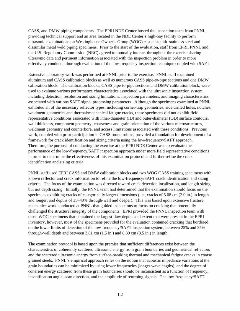
Figure 1.3 Side View of Typical WOG DMW Specimen Specimen “H” was a specially fabricated EPRI pipe section containing a 100% through-wall mechanical fatigue crack and was examined from the SCSS side only. This specimen was a wrought steel pipe to statically cast elbow, where the specimen had actually been broken into two separate pieces at one point, and re-welded (at different depths across the width of the crack). This specimen was 35.71 cm (14.06 in.) in width (circumferential direction), 60.96 cm (24.0 in.) in length (axial direction), and 6.54-cm (2.575-in.) thick at the weld centerline. The weld centerline lies 31.12 cm (12.25 in.) from the elbow end of the specimen. Figure 1.4 depicts this specimen from the underside.

1.7

Figure 1.4 Underside View of Specimen “H”, 100% Through-Wall Crack, 35.56-cm (14.0-in.) Long

1.8

2 Low-Frequency Ultrasonic Data Acquisition

The low-frequency/SAFT-UT inspection system is an automated, computerized UT imaging system designed and developed by PNNL. This study employed an NRC Mobile SAFT-UT inspection system (this system is no longer used). The NRC system was a field-tested system, consisting of several subsystems and components. The pulser produced high voltage pulses that excited the transducer. The internal pulser was not used with the low-frequency system. The receiver conditioned and amplified the received UT response signals. The system allowed the inspector to apply a time varied amplification factor [i.e., electronically generated distance-amplitude correction (DAC)]. The internal receiver was not used with the low-frequency system. The data acquisition subsystem contained the analog-to digital converter. The data processing and storage subsystem performed SAFT processing of raw (unprocessed) UT data. The data display and analysis subsystem displayed the SAFT-UT processed data (A-scans, B-scans, and C-scans) during analysis of UT indications using the graphics workstation features. The low-frequency ultrasonic data acquisition system used at the EPRI NDE Center allowed low-frequency ultrasonic data to be efficiently acquired under rapid, low noise conditions, for a variety of CASS microstructures using a field-ready automated pipe scanner. The schematic in Figure 2.1 illustrates the laboratory system hardware used for ultrasonic data acquisition during the exercise. The data analysis and storage systems are not included in this schematic. As shown in the schematic, the low-frequency data acquisition electronics are coupled to the NRC Mobile SAFT-UT inspection system. The NRC automated pipe scanner was used for accurate and smooth continuous scanning of the search unit through a specified number of points in the X-Y plane, while maintaining low noise conditions. The NRC system was used to acquire (digitize) data and initialize a trigger output to the motor controller and pulse generator, which in turn, was used to sync all instrumentation. The waveform generator was programmed to generate a single cycle sine wave tone burst, at various voltages, for driving the transmit element of the search unit. The low voltage sine wave tone burst output of the arbitrary waveform generator was amplified by a low-frequency, 200 watt, radio frequency (rf) power amplifier, prior to excitation of the search unit. The received signal responses (echoes) were initially amplified by a low-noise, low-frequency, ultrasonic preamplifier, and then bandpass filtered using a PNNL manufactured active filter in order to allow suitable amplification while reducing extraneous low-frequency noise components under 150 kHz and higher frequency noise components over 600 kHz. The preamplified and conditioned signal responses were then amplified by a wideband amplifier and further conditioned using a high pass filtering option to further enhance amplification while minimizing amplifier noise. All signals (excitation pulses and received signal responses) were monitored using a digital oscilloscope, providing the capability to view the trigger and sync pulses, the excitation pulse before and after amplification, and the received signal response just prior to digitization, simultaneously. The oscilloscope also provided linear averaging, and the capability to analyze the frequency characteristics of the A-scan data.

2.1

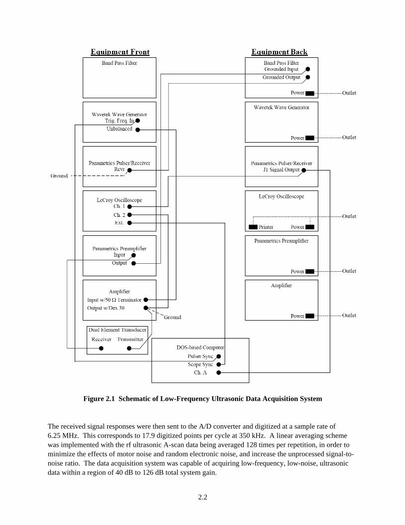
Figure 2.1 Schematic of Low-Frequency Ultrasonic Data Acquisition System The received signal responses were then sent to the A/D converter and digitized at a sample rate of 6.25 MHz. This corresponds to 17.9 digitized points per cycle at 350 kHz. A linear averaging scheme was implemented with the rf ultrasonic A-scan data being averaged 128 times per repetition, in order to minimize the effects of motor noise and random electronic noise, and increase the unprocessed signal-to-noise ratio. The data acquisition system was capable of acquiring low-frequency, low-noise, ultrasonic data within a region of 40 dB to 126 dB total system gain.

2.2

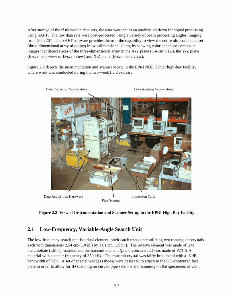
After storage of the rf ultrasonic data sets, the data was sent to an analysis platform for signal processing using SAFT. The raw data sets were post-processed using a variety of beam processing angles, ranging from 6° to 25°. The SAFT software provides the user the capability to view the entire ultrasonic data set (three-dimensional array of points) in two-dimensional slices, by viewing color enhanced composite images that depict slices of the three-dimensional array in the X-Y plane (C-scan view), the Y-Z plane (B-scan end-view or D-scan view) and X-Z plane (B-scan side view). Figure 2.2 depicts the instrumentation and scanner set-up in the EPRI NDE Center high-bay facility, where work was conducted during the two-week field exercise.

Data Acquisition HardwarePipe Scanner

Immersion Tank

Data Collection Workstation Data Analysis Workstation

Data Acquisition HardwarePipe Scanner

Immersion Tank

Data Collection Workstation Data Analysis Workstation

Figure 2.2 View of Instrumentation and Scanner Set-up in the EPRI High Bay Facility 2.1 Low-Frequency, Variable-Angle Search Unit

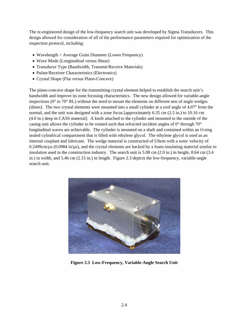
The low-frequency search unit is a dual-element, pitch-catch transducer utilizing two rectangular crystals each with dimensions 2.54 cm (1.0 in.) by 3.81 cm (1.5 in.). The receive element was made of lead metaniobate (LM-1) material and the transmit element (plano-concave cut) was made of PZT 5-A material with a center frequency of 350 kHz. The transmit crystal was fairly broadband with a -6 dB bandwidth of 72%. A set of special wedges (shoes) were designed to attach to the OD-contoured face plate in order to allow for ID scanning on curved pipe sections and scanning on flat specimens as well.

2.3

The re-engineered design of the low-frequency search unit was developed by Sigma Transducers. This design allowed for consideration of all of the performance parameters required for optimization of the inspection protocol, including: • Wavelength > Average Grain Diameter (Lower Frequency) • Wave Mode (Longitudinal versus Shear) • Transducer Type (Bandwidth, Transmit/Receive Materials) • Pulser/Receiver Characteristics (Electronics) • Crystal Shape (Flat versus Plano-Concave)

The plano-concave shape for the transmitting crystal element helped to establish the search unit’s bandwidth and improve its zone focusing characteristics. The new design allowed for variable-angle inspections (0° to 70° RL) without the need to mount the elements on different sets of angle wedges (shoes). The two crystal elements were mounted into a small cylinder at a roof angle of 4.07° from the normal, and the unit was designed with a zone focus [approximately 6.35 cm (2.5 in.) to 10.16 cm (4.0 in.) deep in CASS material]. A knob attached to the cylinder and mounted to the outside of the casing unit allows the cylinder to be rotated such that refracted incident angles of 0° through 70° longitudinal waves are achievable. The cylinder is mounted on a shaft and contained within an O-ring sealed cylindrical compartment that is filled with ethylene glycol. The ethylene glycol is used as an internal couplant and lubricant. The wedge material is constructed of Ultem with a sonic velocity of 0.2499cm/µs (0.0984 in/µs), and the crystal elements are backed by a foam-insulating material similar to insulation used in the construction industry. The search unit is 5.08 cm (2.0 in.) in height, 8.64 cm (3.4 in.) in width, and 5.46 cm (2.15 in.) in length. Figure 2.3 depicts the low-frequency, variable-angle search unit.

Figure 2.3 Low-Frequency, Variable-Angle Search Unit

2.4

3 Signal Processing

Prior to the EPRI exercise, a combination of SAFT and the implementation of an A-scan subtraction algorithm to the data were examined to determine if any signal-to-noise improvement could be made. The A-scan subtraction algorithm subtracts a selected A-scan from every A-scan in the entire data set. “Synthetic aperture focusing” refers to a process in which the focal properties of a large-aperture focused transducer are synthetically generated from data collected over a large area using a small transducer with a divergent sound field. The processing required to focus this collection of data has been called beam forming, coherent summation, or synthetic aperture processing. The resultant image is a full-volume focused characterization of the inspected area. Figure 3.1 depicts Ms. Deborah Jackson (NRC Project Monitor) and Dr. Robert Harris (PNNL) performing SAFT processing on the ultrasonic data and analyzing the processed ultrasonic images. The SAFT processing algorithm is able to provide significant enhancements to the inspection of coarse-grained materials. The resolution of an imaging system is limited by the effective aperture area; that is, the area over which data can be detected, collected, and processed. SAFT is an imaging method that was developed to overcome some of the limitations imposed by large physical apertures and has been successfully applied in the field of ultrasonic testing. Relying on the physics of ultrasonic wave propagation, SAFT is a very robust technique.

Figure 3.1 Data Analysis Being Conducted by Ms. Deborah Jackson (NRC) and Dr. Robert Harris (PNNL)

3.1

Utilizing a pitch-catch configuration for typical data collection throughout the EPRI exercise, the transducer was positioned on the surface of the specimen, and rf ultrasonic data was collected. As the transducer was scanned over the surface of the specimen, the A-scan record (rf waveform) was amplified, filtered, and digitized for each position of the transducer. Each reflector produced a collection of echoes in the A-scan records. The unprocessed or rf data sets were then post-processed using the SAFT algorithm, and invoking a variety of full beam angle values (between 6° and 25°) in order to optimize the spatial averaging enhancement. If the reflector is an elementary single point reflector, the collection of echoes will form a hyperbolic surface within the data-set volume. The shape of the hyperboloid is determined by the depth of the reflector in the specimen and the velocity of sound in the specimen. This relationship, between echo location in the series of A-scans and the actual location of the reflectors within the specimen, makes it possible to reconstruct a high-resolution, high signal-to-noise ratio image from the acquired raw data. If the scanning and surface geometries are well known, it is possible to accurately predict the shape of the locus of echoes for each point within the test object. The process of coherent summation for each image point involves shifting a locus of A-scans, within a regional aperture, by predicted time delays and summing the shifted A-scans. This process may also be viewed as performing a spatial matched filter operation for each point within the volume to be imaged. Each element is then averaged by the number of points that were summed to produce the final processed value. If the particular location correlates with the elementary point response hyperboloid, then the values summed will be in phase and produce a high-amplitude result. If the location does not correlate with the predicted response, the destructive interference will take place and the spatial average will result in a low-amplitude value; thus, reducing the noise level to a very small value. The A-scan subtraction method was implemented for data analysis by selecting and subtracting one A-scan from all other A–scans in the data set. This worked best for rf data sets, not rectified data sets. It appeared to be very effective in removing “shoe noise” and other constant-time signals. However, SAFT is equally effective at removing constant-time signals that are not near the front surface, and sub-volume selection readily removes near-surface signals. On one specimen, the following process improved the flaw visibility: • Perform unrectified SAFT (i.e., no envelope detection) • Perform A-scan selection and subtraction • Perform rectification of the data set

However, this technique was used on a second data set with no improvement. In order to test this process, it would be best to automate the sequence of steps, as it presently requires using several programs alternately and is quite time-consuming. The conclusion was to utilize a wide-angle (beam-processing angle) SAFT-processing scheme for the EPRI exercise. 3.1 Examination Procedures

The inspection system was configured to accommodate data acquisition for a variety of component geometries and sizes, including:

3.2

• Pipe to pipe sections • Pipe to elbow sections • Outlet nozzle to safe end to elbow sections • Pipe to safe end to RPV outlet nozzle sections • Pipe to safe end to RPV inlet nozzle section • DMW sections • Calibration standards

The specimens were loaded into a plastic immersion tank with a water bath for couplant. Each component was examined using the following orientations: • 0° L-wave, 350 kHz for back surface profiling over the entire weld area • 30° L-wave, 250, 350, and 450 kHz both near and far-side scanning • 45° L-wave, 250, 350, and 450 kHz both near and far-side scanning • 60° L-wave, 250, 350, and 450 kHz both near and far-side scanning

Initially, all three examination frequencies were used; however, due to the higher attenuation at 450 kHz, the fact that no significantly useful information was added by performing scans at 450 kHz, and the additional data acquisition and analysis time consumed by using a third inspection frequency, this frequency was eliminated after the first two WOG specimen examinations. Therefore, 13 full scans were conducted per component, unless the component geometry, weld crown, or surface area precluded the use of 30° or 60° incident angles. All data was post-processed using the SAFT signal processing algorithm with a 25° beam processing angle and at times a 6° and/or 12° beam processing angle. Step size for each scan was 2.54 mm (0.1 in.) per increment in both axes. Digitization sample rate was 6.25 MHz, yielding approximately 18 digitized points per cycle during data acquisition for 350-kHz signals. The number of data points per inch along the sound propagation direction was approximately 40 points (corresponding to approximately a 1-mm sample spacing). With the given step size, sample rate, and a reasonable digitized time window of 50 to 60 µs at each point, over the spatial area and volume scanned all individual files were under 5 Mbytes in total size. Each file was named with a filename that identified the component scanned, the incident angle, the examination frequency, the microstructure, and near or far side scanning orientation. All raw UT data files and SAFT processed files were saved to a re-writable magneto-optical 1.2 Gbyte disk and 1 Gbyte Jazz Diskettes for storage and later analysis. Prior to scanning it was necessary to measure the acoustic velocity in the specimen at 0° and, if possible, at 30°, 45°, and 60° using the end of block (corner trap geometry) as the target. The end of block geometry was also used as a target indicator for identification and selection of the proper incident angle in the material under test. Specimen thicknesses were measured, surface contour sketches were drawn, and a velocity template was completed for each specimen at each incident angle for each microstructure. The velocity and specimen information templates are shown in Appendix A. Scanning was invoked from the OD surface. General scanning procedures include: 1. Invoke scanning setup menu on PC 2. Modify header files and parameters for transducer, material, sampling, and scan pattern 3. Examine A-scan trace on computer monitor

3.3

4. Slowly scan transducer over corner trap geometry and/or welded area and verify proper gain settings

on instrumentation, setting the total system gain 2 dB below saturation of the highest amplitude signal to be found

5. When all parameters have been set, outline scan aperture 6. Print out header file 7. Initiate scanning 8. Complete documentation of “Instrumental Settings” template. This template, along with other

pertinent recording documentation, is shown in Appendix A. 3.2 Crack Identification and Sizing Criteria

Within any given planar view (B-scan side view, B-scan end view, or C-scan view), the analysis focused on the following criteria for identifying or rejecting regions as cracked in the material, where ultrasonic signal amplitude anomalies occurred. Signal amplitude anomalies will be abbreviated as SAAs in the following criteria description. These criteria are based upon acquiring some combination of redundancy in the ultrasonic data as a function of the various inspection parameters which include examination incident angle, driving frequency of the transducer, and scan direction. The diagram in Figure 3.2 illustrates the area of interest for crack identification as it relates to component geometry. SAAs occurring in the volumetric space between the top edges of the two counterbore slopes, and including the weld root, will be fully examined. This is due primarily to the high-amplitude signal returns scattered from counterbore geometry effectively masking any cracking that may exist in this area.

E lb o w P ip e

T o p “ t ip ” o f c o u n te rb o re

W e ld r o o t

O D S u r fa c

ID S u r f a c e

A r e a o f In te r e s t f o r E P R I E x e r c is e

T T

X

Z o n e th a t C o d e s a y s m u s t b e in s p e c te d is d e f in e d b y T = th ic k n e s s a n d X = 1 /3 le n g th

Area of Interest for EPRI Exercise

PipeOD Surface

ID Surface

Zone that Code says must be inspected isdefined by T = thickness and X = 1/3 lengthTop “tip” of counterbore

Weld root

ElbowE lb o w P ip e

T o p “ t ip ” o f c o u n te rb o re

W e ld r o o t

O D S u r fa c

ID S u r f a c e

A r e a o f In te r e s t f o r E P R I E x e r c is e

T T

X

Z o n e th a t C o d e s a y s m u s t b e in s p e c te d is d e f in e d b y T = th ic k n e s s a n d X = 1 /3 le n g th

Area of Interest for EPRI Exercise

PipeOD Surface

ID Surface

Zone that Code says must be inspected isdefined by T = thickness and X = 1/3 lengthTop “tip” of counterbore

Weld root

Elbow

Figure 3.2 Illustration Defining the “Area of Interest” for Crack Definition

3.4

1. If the full complement of inspection angles were used in the examination (0°, 30°, 45°, and 60°), coinciding SAAs should occur from at least one inspection angle from both sides of the weld, in order for the indication to be further considered as evidence of cracking. Exceptions may be made to this, if for instance strong SAAs are evident from only one side due to unusual material or surface conditions on the adjacent side precluding the acquisition of useable data.

2. If the full complement of inspection angles were used in the examination, coinciding SAAs must

occur at more than one examination frequency, or more than one examination incident angle, or more than one scan direction (from data acquired from the other side of the weld), or some combination thereof, in order to establish a degree of redundancy that allows the inspection analysis to determine whether or not the SAA is evidence of cracking.

3. SAAs may occur above, on, or below the back surface line appearing on the SAFT representations.

Differences in position of ±1.27 cm (±0.5 in.) above or below this line are not significant, and SAA position will be measured from the peak amplitude point. When an SAA occurs in this region, its tail will be included in the boxed examination region of the image. When the back-surface line is positioned accurately, corner trap signal returns from cracking in the material will result in SAAs that lie just on the back-surface line, with the majority of the SAA below the line. The accuracy of the back-surface line is a function of the material velocity and transducer delay, and the actual position of an SAA relative to this line is a function of incident angle, acoustic velocity, frequency, wavelength, and zone focal dimensions of the transducer. Because material velocity varies with spatial position and incident angle in the material, inaccuracies must be allowed for. The 0° data acquired from both sides of the weld is used to determine ID surface contouring, and nominal wall thickness data is used to substantiate the ultrasonic data on the SAFT images. Depending upon the differences between the nominal wall thickness data and the 0° ultrasonic profiling data, the actual z-axis dimension of the volume boxed for examination can range up to 3.81 cm (1.5 in.) in total length.

4. SAAs should have some degree of characteristic shape (either circular or elliptical) to them, with

somewhat smooth contours on their edges, as opposed to random blotchy, scattered amplitude blips that appear with little symmetry and rough contours. Also, SAAs should have reasonable and proper orientation with respect to the examination incident angle of the insonifying beam. A perpendicular orientation is preferred.

5. SAAs occurring very near the edge of the material under test (especially in the case of curved pipe

sections) will be discounted due to edge scattering effects. The side wall of the pipe section acts as a mirror to reflect more energy back to the receive element than would normally occur if no edge existed. This can be minimized by starting the transducer at a point on the pipe OD surface where no overlap exists between the transducer face and the edge of the pipe, but this effectively decreases the width of the scan on the ID surface.

6. Differences in lateral position of ±1.27 cm (±0.5 in.) or less are not significant, except at a single

examination incident angle with multiple frequencies. 7. Length and depth sizing will be performed from the most continuous SAFTed image where the

signal-to-noise ratio is high, if a data file of this nature exists; however, in most cases, the composite data will be plotted using spreadsheet analysis and data resolution of 2.54 mm (0.1 in.) in the x- and

3.5

y-axes. If tip signal returns exist, depth measurements will be made using the most continuous SAFTed image. In the case of length sizing and localization (positioning), the -3 dB points will be used to “clip” the data from the background noise, and the data points will be extracted from the SAFT images and plotted on a spreadsheet. Generally, the accuracy of length sizing and crack positioning will be ±1.27 cm (±0.5 in.) in both circumferential and axial directions. If one data file exhibits a strong signal-to-noise ratio and the SAA of interest is coincident in other scans, this data file may be used for location and sizing; however, in general when no single data file can be judged to exhibit these characteristics, the composite data will be plotted, and the data will be averaged graphically in order to determine location and size.

8. PNNL inspection analysis will provide sizing and location data that is referenced to the OD surface

dimensions, and will compensate for transducer overlap and nominal beam position in the material. EPRI personnel will need to compensate for true state crack dimension data reference to the ID surface of the component.

The data analysis protocol conducted at EPRI utilized multiple data sets for crack identification, localization and sizing. The analysis technique (which is presently quite time-intensive) is based upon redundancy of the ultrasonic indications as a function of the various inspection parameters. Scans were performed at various angles and frequencies and, when possible, from both sides of the weld. Each scan was separately analyzed for indications. Each indication was given a start and stop pair of (x, y) coordinates. These coordinates were entered in an Excel spreadsheet. The different scans were placed in different columns so that Excel could automatically assign colors and symbols to the respective scans. Three (x, y) plots of the data sets were made from one side of the weld, from the other side of the weld, and both sides combined. 3.3 Examination Results

In the work leading up to the EPRI exercise, it had been determined that the low-frequency/SAFT inspection system could consistently detect geometrical reflectors, notches (25% deep), sawcuts (25% deep), side-drilled holes (1/8 T), and fatigue-type cracking in thinner-walled CASS materials that were at least 30–35% through-wall in depth and greater, and with a minimal extent of 2.54 cm (1.0 in.) or longer. The plots were examined visually to determine what indications appeared to recur most often, which (if any) were geometrical features, and which seemed to be grain noise or other irrelevant indications. The most likely cluster was used to determine the crack location. In some cases an arithmetic average of the endpoints was used; in other cases, a visual estimate was used. This has the advantage of allowing the inspector to assign (implicit) weights to the data sets. The PNNL inspection team was ideally looking to examine fatigue cracks in CASS material with depth dimensions of 35–40% or greater and length dimensions of 5.08 cm (2.0 in.) or greater. The actual flaw depths and flaw lengths are given below in Table 3.1.

3.6

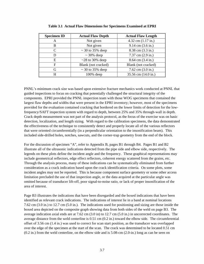
Table 3.1 Actual Flaw Dimensions for Specimens Examined at EPRI

Specimen ID Actual Flaw Depth Actual Flaw Length A Not given 4.32 cm (1.17 in.) B Not given 9.14 cm (3.6 in.) C ~ 30 to 35% deep 8.38 cm (3.3 in.) D ~ 30% deep 7.37 cm (2.9 in.) E ~28 to 30% deep 8.64 cm (3.4 in.) F Blank (not cracked) Blank (not cracked) G ~ 30 to 35% deep 7.62 cm (3.0 in.) H 100% deep 35.56 cm (14.0 in.)

PNNL’s minimum crack size was based upon extensive fracture mechanics work conducted at PNNL that guided inspections to focus on cracking that potentially challenged the structural integrity of the components. EPRI provided the PNNL inspection team with those WOG specimens that contained the largest flaw depths and widths that were present in the EPRI inventory; however, most of the specimens provided for the evaluation contained cracking that bordered on the lower limits of detection for the low-frequency/SAFT inspection system with regard to depth, between 25% and 35% through-wall in depth. Crack depth measurement was not part of the analysis protocol, as the focus of the exercise was on basic detection, localization, and length sizing. With regard to the calibration specimens, the data demonstrated the effectiveness of the technique to consistently detect and properly locate all of the various reflectors that were oriented circumferentially (in a perpendicular orientation to the insonification beam). This included side-drilled holes, notches, sawcuts, and the corner-trap geometry from the end of the block. For the discussion of specimen “A”, refer to Appendix B, pages B1 through B4. Pages B1 and B2 illustrate all of the ultrasonic indications detected from the pipe side and elbow side, respectively. The legends on these plots define the incident angle and the frequency. These graphical representations may include geometrical reflectors, edge effect reflectors, coherent energy scattered from the grains, etc. Through the analysis process, many of these indications can be systematically eliminated from further consideration as a crack indication based upon the crack identification criteria. On some plots, some incident angles may not be reported. This is because component surface geometry or some other access limitation precluded the use of that inspection angle, or the data acquired at the particular angle was omitted because of transducer lift-off, poor signal-to-noise ratio, or lack of proper insonification of the area of interest. Page B3 illustrates the indications that have been disregarded and the boxed indications that have been identified as relevant crack indications. The indications of interest lie in a band at nominal locations 7.62 cm (3.0 in.) to 12.7 cm (5.0 in.). The indications used for positioning and sizing are those inside the boxed area depicted on the composite graph showing data from both sides of the weld on page B3. The average indication axial ends are at 7.62 cm (3.0 in) to 12.7 cm (5.0 in.) in uncorrected coordinates. The average distance from the weld centerline is 0.51 cm (0.2 in.) toward the elbow side. The circumferential offset of 3.56 cm (1.4 in.) was used to correct for scan start position, as the transducer was overlapped over the edge of the specimen at the start of the scan. The crack was determined to be located 0.51 cm (0.2 in.) from the weld centerline, on the elbow side and is 5.08-cm (2.0-in.) long as can be seen on

3.7

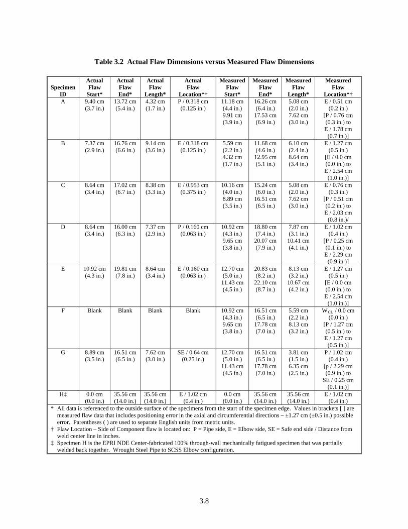
Table 3.2 Actual Flaw Dimensions versus Measured Flaw Dimensions

Specimen ID

Actual Flaw

Start*

Actual Flaw End*

Actual Flaw

Length*

Actual Flaw

Location*†

Measured Flaw

Start*

Measured Flaw End*

Measured Flaw

Length*

Measured Flaw

Location*† A 9.40 cm

(3.7 in.) 13.72 cm (5.4 in.)

4.32 cm (1.7 in.)

P / 0.318 cm (0.125 in.)

11.18 cm (4.4 in.) 9.91 cm (3.9 in.)

16.26 cm (6.4 in.)

17.53 cm (6.9 in.)

5.08 cm (2.0 in.) 7.62 cm (3.0 in.)

E / 0.51 cm (0.2 in.)

[P / 0.76 cm (0.3 in.) to E / 1.78 cm

(0.7 in.)] B 7.37 cm

(2.9 in.) 16.76 cm (6.6 in.)

9.14 cm (3.6 in.)

E / 0.318 cm (0.125 in.)

5.59 cm (2.2 in.) 4.32 cm (1.7 in.)

11.68 cm (4.6 in.)

12.95 cm (5.1 in.)

6.10 cm (2.4 in.) 8.64 cm (3.4 in.)

E / 1.27 cm (0.5 in.)

[E / 0.0 cm (0.0 in.) to E / 2.54 cm

(1.0 in.)] C 8.64 cm

(3.4 in.) 17.02 cm (6.7 in.)

8.38 cm (3.3 in.)

E / 0.953 cm (0.375 in.)

10.16 cm (4.0 in.) 8.89 cm (3.5 in.)

15.24 cm (6.0 in.)

16.51 cm (6.5 in.)

5.08 cm (2.0 in.) 7.62 cm (3.0 in.)

E / 0.76 cm (0.3 in.)

[P / 0.51 cm (0.2 in.) to E / 2.03 cm

(0.8 in.)/ D 8.64 cm

(3.4 in.) 16.00 cm (6.3 in.)

7.37 cm (2.9 in.)

P / 0.160 cm (0.063 in.)

10.92 cm (4.3 in.) 9.65 cm (3.8 in.)

18.80 cm (7.4 in.)

20.07 cm (7.9 in.)

7.87 cm (3.1 in.)

10.41 cm (4.1 in.)

E / 1.02 cm (0.4 in.)

[P / 0.25 cm (0.1 in.) to E / 2.29 cm

(0.9 in.)] E 10.92 cm

(4.3 in.) 19.81 cm (7.8 in.)

8.64 cm (3.4 in.)

E / 0.160 cm (0.063 in.)

12.70 cm (5.0 in.)

11.43 cm (4.5 in.)

20.83 cm (8.2 in.)

22.10 cm (8.7 in.)

8.13 cm (3.2 in.)

10.67 cm (4.2 in.)

E / 1.27 cm (0.5 in.)

[E / 0.0 cm (0.0 in.) to E / 2.54 cm

(1.0 in.)] F Blank Blank Blank Blank 10.92 cm

(4.3 in.) 9.65 cm (3.8 in.)

16.51 cm (6.5 in.)

17.78 cm (7.0 in.)

5.59 cm (2.2 in.) 8.13 cm (3.2 in.)

WCL / 0.0 cm (0.0 in.)

[P / 1.27 cm (0.5 in.) to E / 1.27 cm

(0.5 in.)] G 8.89 cm

(3.5 in.) 16.51 cm (6.5 in.)

7.62 cm (3.0 in.)

SE / 0.64 cm (0.25 in.)

12.70 cm (5.0 in.)

11.43 cm (4.5 in.)

16.51 cm (6.5 in.)

17.78 cm (7.0 in.)

3.81 cm (1.5 in.) 6.35 cm (2.5 in.)

P / 1.02 cm (0.4 in.)

[p / 2.29 cm (0.9 in.) to

SE / 0.25 cm (0.1 in.)]

H‡ 0.0 cm (0.0 in.)

35.56 cm (14.0 in.)

35.56 cm (14.0 in.)

E / 1.02 cm (0.4 in.)

0.0 cm (0.0 in.)

35.56 cm (14.0 in.)

35.56 cm (14.0 in.)

E / 1.02 cm (0.4 in.)

* All data is referenced to the outside surface of the specimens from the start of the specimen edge. Values in brackets [ ] are measured flaw data that includes positioning error in the axial and circumferential directions – ±1.27 cm (±0.5 in.) possible error. Parentheses ( ) are used to separate English units from metric units.

† Flaw Location – Side of Component flaw is located on: P = Pipe side, E = Elbow side, SE = Safe end side / Distance from weld center line in inches.

‡ Specimen H is the EPRI NDE Center-fabricated 100% through-wall mechanically fatigued specimen that was partially welded back together. Wrought Steel Pipe to SCSS Elbow configuration.

3.8

page B4. It starts at 11.18 cm (4.4 in.) from the edge of the part and stops at 16.26 cm (6.4 in.). All measurements were made from the OD, and the positioning error associated with this data is ±1.27 cm (±0.5 in.) in both the axial and circumferential directions. The presentation on page B4 also shows the true location of the crack referenced to the OD surface of the pipe, superimposed on the measured data. For tutorial purposes, the data associated with specimen “B” has been presented in a detailed step-by-step fashion that takes the reader through the various stages of the analysis using the SAFT-processed ultrasonic images. Refer to Appendix C, pages C1 through C10, for this portion of the discussion. Page C1 illustrates the C-scan view of specimen “B” at 30° incidence using 250 kHz from the pipe side of the weld. The color bar located on the right side of the image is a relative amplitude scale in decibels (dB), defining the dynamic range of the scan. The brighter colors (pink and red) define higher-amplitude signal returns while the darker colors (blue and black) define lower-amplitude signal returns. The various ultrasonic indications shown on the C-scan view are labeled with an associated description. The top of the image is the scan start position of the transducer at the “0” position in the circumferential direction. The nominal weld center line is illustrated by the large tick mark on the bottom of the image and is defined as the “0” position in the axial direction. All C-scan images are defined in this manner. The ultrasonic indications are boxed out (isolated), magnified, and analyzed using various perspectives (B-scan side view, B-scan end view, and C-scan view) to determine various characteristics associated with the specific signal amplitude anomaly. These include shape, contour, extent, axial position with respect to the weld centerline, depth with respect to the back-surface line, orientation with respect to the insonification beam, etc. Figure C1 shows ultrasonic indications due to weld geometry, material reflectors (large grain boundaries), and the crack itself (relevant indication). The analysis is performed as a function of examination frequency, incident angle, and scan direction with respect to the weld. Therefore, numerous views are studied and dissected using isolation boxes and magnification. This process was quite time-intensive. Improvements have since been made that dramatically improved processing time. Page C2 illustrates the same view C-scan view only the entire data set has been “clipped” by -3 dB so that only the relatively higher-amplitude signal responses are shown, and the surrounding background signal levels are reduced. This enhanced image can separate indications for localization and sizing. Pages C3 and C4 show the same view from data sets scanned at 45° incidence and 60° incidence using 350 kHz. Again, the -3 dB “clip” is used. At these angles and this specific frequency, different geometric indications are evident, and what are considered relevant indications (labeled after the analysis was completed) and various material reflectors can also be seen. Initially, all indications are plotted, and no one indication is deemed “relevant” until the composite data is reviewed and the criteria for crack identification and sizing are met. For tutorial purposes, the “relevant” indications are labeled for the readers benefit. Page C5 depicts the C-scan view of specimen “B” scanned at 30° from the elbow side of the weld using 350 kHz. This data set was SAFT-processed with envelope detection, and then the A-scan subtraction algorithm was invoked, which proved quite useful on this particular data set, as it provided good separation between the relevant ultrasonic indications and the ultrasonic indications from the counterbore. The relevant indications stand out nicely from the background noise in the image. Page C6 shows a boxed (isolated) and magnified region from the previous C-scan, that illustrates the relevant indications with better definition. Page C7 shows the same data set and the same C-scan perspective only the data set

3.9

used to generate this image was processed using SAFT with no A-scan subtraction performed. Pages C8 and C9 show another comparison of identical data sets (45° incidence at 250 kHz from the elbow side) using SAFT alone, and non-envelope detected SAFT combined with A-scan subtraction, respectively. This time, there is not much improvement with regard to sign-to-noise or image definition. These images illustrate edge effects, material reflectors and relevant indications as well. Page C10 illustrates the C-scan view of specimen “B” as scanned at 45° from the elbow side of the weld at 450 kHz. Again, this shows indications from material grain boundaries, energy scattered from the edge (side-wall) of the specimen, and coherent energy scattered from the flaw itself (relevant indication). This view has been clipped using the -3 dB method. These types of ultrasonic images allow the inspector to examine various planar perspectives (side views and end views) of the data scanned from different sides of the weld. From these B-scan perspectives, the analyst can see the signal amplitude responses separated from the front surface (including show noise). Some of these images were generated using the -3 dB clip method for better separation of indications. The inspector can also generate B-scan side views (composite views of the component in the X-Z plane and B-scan end views (composite orthogonal side views) of the component in the Y-Z plane. From these B-scan perspectives, the analyst can gain new insights into the position and characteristics of the various signal amplitude indication. After reviewing all of the various images (as a function of frequency, incident angle and scan direction) and plotting all of the indications on a composite map, the area of highest redundancy is then used to determine crack location and extent. For the general discussion of specimen “B” and referring to Appendix B, pages B5 through B8, the relevant indications are those within the boxed area depicted on the composite graph showing data from both sides of the weld. The measured crack location has been corrected to probe offset in the circumferential direction. The view is from the OD. All measured crack data are ±1.27 cm (±0.5 in.) in both the axial and circumferential directions. The plot on page B7 shows a high degree of redundancy among the various incident angles and frequencies in the boxed area. From the data, the crack is located 1.27 cm (0.5 in.) from the weld centerline and 6.10-cm (2.4-in.) long. The measured crack begins at 5.59 cm (2.2 in.) and runs to 11.68 cm (4.6 in.) circumferentially as shown on page B8. It should be noted that this technique may be detecting only the deepest portions of the crack and not those portions of the crack that lie outside of the detection limits of the system. For the discussion of specimen “C”, refer to Appendix B, pages B9 through B12. The individual indications for the pipe side and elbow side data are shown on pages B9 and B10. The white box indicates the region of relevant indications as shown on the plot on page B11. There are two large groups of indications from the elbow side, and numerous scattered indications from the pipe side. The upper group of indications from the elbow side have only three similar indications, while the lower group has seven. The lower group also shows indications from other angles and the other side. To convert the above measurements to part coordinates, an offset of 3.56 cm (1.4 in.) was added to the circumferential values in order to compensate for transducer offset. The crack is estimated to be 5.08-cm (2.0-in.) long, on the elbow side, 0.76 cm (0.3 in.) from the weld centerline, beginning 10.16 cm (4.0 in.) from the edge of the block and ending 15.24 cm (6.0 in.) from the edge of the block, in the circumferential direction. All measurements are ±1.27 cm (±0.5 in.). The plot on page B12 shows the general positioning, as viewed from the OD. All measurements were calculated from the OD. For the discussion of specimen “D”, refer to Appendix B, pages B13 through B16. Pages B13 and B14 show all of the ultrasonic indications on the pipe side and elbow side, each one reduced to two -3 dB

3.10

points, one at either end of the circumference direction. From the composite view on page B15, the indications to the left of the weld centerline appear to be geometric in nature. The 30° data from the pipe side and the 60° data from the elbow side did not yield useful data and were omitted. There was not a single obvious indication on any one scan, so the area of greatest repetition has been indicated as the most probable location of the crack. The selected area enclosed by a white box on page B15 shows multiple indications from both sides of the weld and redundant ultrasonic contributions from multiple incident angles, which is not the case with any other area. Page B16 shows the crack measurement. The measured crack is 7.87-cm (3.1-in.) long and is located 1.02 cm (0.4 in.) from weld centerline, on the elbow side. It starts at 10.92 cm (4.3 in.) from the edge (OD side up, 0 at bottom, elbow end at right) and ends at 18.80 cm (7.4 in.) in the circumferential direction. All estimates are as measured from the OD, ±1.27 cm (±0.5 in.). For discussion of specimen “E”, refer to Appendix B, pages B17 through B22. Pages B17 and B18 show all of the ultrasonic indications on the pipe side and elbow side, each one reduced to two -3 dB points, one at either end of the indication. Page B19 shows a composite plot with all of the indications from both sides of the weld. From the entire set of indications shown on this plot, the indications that appear to be geometric (45° indications to the left of the weld centerline) were eliminated from consideration. A reduction in the data based upon the crack identification criteria resulted in a plot shown on page B20, where the indications in the boxed area were identified as the relevant indications. From this, the indications from the 60° scan were eliminated, as having no coincident indications from other frequencies at or near the same axial position. The other indications starting at about 5.08 cm (2.0 in.) to 7.62 cm (3.0 in.) on the circumferential axis were eliminated for the same reason. This left the indications in the boxed area on the plot on page B21, which show coincident information from 45° in both directions, and 30° from one direction (the only 30° scan that could be made). The final call is shown on page B22 where all measurements are ±1.27 cm (±0.5 in.). The crack is located 1.27 cm (0.5 in.) from the weld centerline on the elbow side, and is 8.13 cm (3.2-in.) long. It begins at 16.26 cm (6.4 in.) from the edge of the part 12.7 cm (5.0 in.) on the scanning axis, plus 3.56 cm (1.4 in.) offset due to transducer overlap. It continues to 24.38 cm (9.6 in.) from the edge of the part in the circumferential direction. For discussion of specimen “F”, refer to Appendix B, pages B23 through B24. The 45° scans used to examine this component were uncalibrated and could not be heavily relied upon. Page B23 shows the composite information, which is from one side only. The nominal coordinates of the measured indication are shown on page B24. The actual weld centerline, which was very difficult to determine, appears to be about -2.03 cm (-0.8 in.), judging by the 30° data, so the crack position is actually on the weld centerline. The 30° data appeared to exhibit a higher signal-to-noise ratio than the 45° data, and was used to determine the position and length of the indication. All coordinates are ±1.27 cm (±0.5 in.). The indication is on the weld centerline and is 5.59-cm (2.2-in.) long. It begins at 15.24 cm (6.0 in.) from the sample edge [10.92 cm (4.3 in.) + 4.32 cm (1.7 in.) offset due to transducer position] and ends at 20.83 cm (8.2 in.) in the circumferential direction. The plot on page B24 shows the analysis results in part coordinates as seen from the OD surface. Specimen “F” (the uncracked specimen) was called cracked only because of the limited amount of ultrasonic data acquired. EPRI personnel would not permit examination from the wrought steel side of the weld, and the OD and ID contour on the SCSS side of the weld did not allow the inspectors to calibrate the search unit properly or measure velocity as a function of incident angle. A surface lip on the OD precluded the use of 60° examination, and the 45° examination was not optimal due to the lack of a

3.11

reflector target for proper angle selection. Although two different scans were acquired at 45°, neither data set was optimal. The information reported on this specimen was based upon data that could not be identified as part geometry or cracked material. The analysis was contingent upon using limited data from only one side of the weld, and the required degree of redundancy as a function of scan direction and examination angles did not exist. Part geometry could not be localized or properly positioned. From the information that was acquired, the PNNL team decided to call the ultrasonic indications as a “crack” solely based upon this limited information. Prior to obtaining knowledge of the true-state of this specimen, the PNNL team did state that under normal conditions, no call would have been made on this specimen until further data could be acquired to show some redundancy and to support the proper location of part geometry. After further analysis (using data acquired from both sides of the weld), the call on this specimen would have indeed been “blank”. For the discussion of specimen “G”, refer to Appendix B, page B25. This specimen could be scanned from only one side and at two angles; 45° and 60°. There was only one consistent indication, as seen from the C-scan views in the ultrasonic data. The average of four of the five scans was used for location and sizing of this indication. All locations were ±1.27 cm (±0.5 in.). The crack is located 1.02 cm (0.4 in.) from the weld centerline, on the pipe side, and is 3.81 cm (1.5-in.) long. The crack begins at 12.7 cm (5.0 in.) from the edge of the specimen and runs to 16.51 cm (6.5 in.), this takes into account an offset of 2.95 cm (1.16 in.) from the edge of the part due to transducer overlap. With the limited information, and the lack of proper placement of part geometry due to limited data acquisition, the error in axial positioning with respect to the weld centerline should be disregarded. Specimen “H” did not allow the inspectors the luxury of using the end-of-block corner trap for calibration of the incident angle and velocity measurements in the material; therefore, the actual crack was used to “dial” in the proper incident angle and make the necessary velocity measurements prior to scanning. This did not affect the quality of the ultrasonic data, as the crack was detected along its full length from start to finish of the entire scan aperture. Crack location was measured correctly, and the areas of higher and lower amplitude in the C-scan views were verified by EPRI personnel as corresponding to the varying degrees of weldment associated with circumferential location along the crack as is evident in the B-scan views. A graphic presentation of inspection results, showing positions as estimated ultrasonically compared with true positions, is shown in Figure 3.3. Results are laid out as though all the defects were on a single piece, with weld centerlines spaced 5.08 cm (2.0 in.) apart. Sample “F” was a false cell, so no true position is shown.

3.12

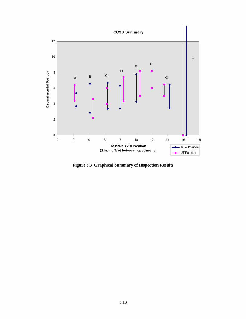
CCSS Summary

0

2

4

6

8

10

12

0 2 4 6 8 10 12 14 16

Relative Axial Position(2 inch offset between specimens)

Circ

umfe

rent

ial P

ositi

on

18

True Position

UT Position

A G

ED

CB

HF

Figure 3.3 Graphical Summary of Inspection Results

3.13

3.14

4 Conclusions

The work conducted at PNNL and during the EPRI field exercise demonstrated the potential for useful crack detection in CASS and DMW materials using low-frequency ultrasound. Specifically, an ultrasonic inspection technique coupled with SAFT signal processing, utilizing the full complement of examination angles (0°, 30°, 45°, and 60° from both sides of the weld) in the longitudinal wave mode, in a pitch-catch configuration at low frequencies (250 to 450 kHz) has demonstrated a good probability of detection for fatigue cracking in coarse-grained stainless steel. Utilization of the synthetic aperture focusing technique for signal processing coupled with the low-frequency UT technique in a field test at the EPRI NDE Center provided positive results with respect to detection, localization, and length sizing. The experimental results indicate that this low-frequency/SAFT technique is capable of consistently detecting and sizing circumferentially oriented thermal and mechanical fatigue cracks on the order of 35% deep and greater, and 3.81 cm (1.5 in.) in extent and longer, in CASS and DMW components, as well as fabricated 10% deep circumferential notches, 25% deep circumferential sawcuts, end-of-block corner traps, and 1.59-mm (1/16-in.) diameter circumferential side-drilled holes. The results provided in this report do not represent data from a statistically large number of field-representative CASS samples. Approximately 20 CASS specimens (PNNL and WOG specimens) were examined using this inspection protocol. This work clearly demonstrated, however, that the low-frequency/SAFT inspection technique is capable of providing quality detection and localization data, and accurate length sizing information. The follow-on efforts resulting from this initial work are described in NUREC/CR-6929 and NUREG/CR-6933. Significant improvements have been made to the techniques and, in particular, through the use of the low-frequency phased arrays. A non-rigorous statistical and graphical analysis of results for the WOG samples was undertaken in order to more fully understand the data acquired throughout the exercise. Generally speaking, for a perfect fit, the equations for the data would be: y = 1.0x + 0.0 (slope of the best fit line) R2 = 1.0 (correlation coefficient) If R2 is less than 0.5, the correlation is not generally considered causative. In studying the true lengths of the flaws versus the ultrasonically estimated lengths, the data is well correlated especially with the long through-wall crack added to the data set. Figure 4.1 illustrates the fit and shows that the correlation is near 1 for this data. The data for the true center circumferential positions of flaws in the WOG specimens versus the ultrasonically estimated circumferential center positions of these flaws is shown in Figure 4.2. The statistical analysis included three attempts to capture the circumferential aspect of the data acquired at the EPRI NDE Center, and these plots are shown in Figures 4.3 through 4.5.

4.1

Lengths

y = 1.0408x - 0.7443R2 = 0.9704

0

1

2

3

4

5

6

7

8

9

10

11

12

13

14

0 2 4 6 8 10 12 1

True length (surface)

UT

Estim

at

4

e

True Length (surface)

UT

Estim

ate

Lengths

y = 1.0408x – 0.7443R2 = 0.9704

Lengths

y = 1.0408x - 0.7443R2 = 0.9704

0

1

2

3

4

5

6

7

8

9

10

11

12

13

14

0 2 4 6 8 10 12 1

True length (surface)

UT

Estim

at

4

e

True Length (surface)

UT

Estim

ate

Lengths

y = 1.0408x – 0.7443R2 = 0.9704

Figure 4.1 True Surface Length of WOG Specimen Flaws versus Ultrasonically Estimated Lengths.

Units in inches, where 1 inch is equal to 2.54 cm.

y = 0.9609x + 0.458R2 = 0.5207

2

3

4

5

6

7

8

9

10

2 3 4 5 6 7 8 9 1

True Center (surface)

UT

Estim

ate

0

UT

Estim

ate

y = 1.9609x + 0.458R2 = 0.5207

True Center (surface)

Circumferential Positions (center)

y = 0.9609x + 0.458R2 = 0.5207

2

3

4

5

6

7

8

9

10

2 3 4 5 6 7 8 9 1

True Center (surface)

UT

Estim

ate

0

UT

Estim

ate

y = 1.9609x + 0.458R2 = 0.5207

True Center (surface)

Circumferential Positions (center)

Figure 4.2 Circumferential Flaw Center Position on Surface (True versus UT Estimate). Units in inches, where 1 inch is equal to 2.54 cm.

4.2

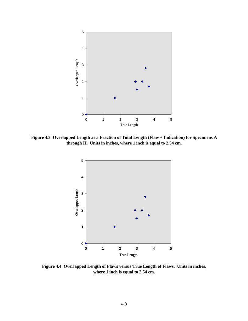
True Length

0

1

2

3

4

5

0 1 2 3 4 5

True length

Ove

rlapp

ed le

ngth

Ove

rlapp

ed L

engt

h

True Length

0

1

2

3

4

5

0 1 2 3 4 5

Ove

rlapp

ed L

engt

h

True LengthTrue Length

0

1

2

3

4

5

0 1 2 3 4 5

True length

Ove

rlapp

ed le

ngth

Ove

rlapp

ed L

engt

h

True Length

0

1

2

3

4

5

0 1 2 3 4 5

Ove

rlapp

ed L

engt

h

True Length Figure 4.3 Overlapped Length as a Fraction of Total Length (Flaw + Indication) for Specimens A

through H. Units in inches, where 1 inch is equal to 2.54 cm.

True Length

Ove

rlapp

edLe

ngth

0

1

2

3

4

5

0 1 2 3 4 5

True Length

Ove

rlapp

edLe

ngth

0

1

2

3

4

5

0 1 2 3 4 5

Figure 4.4 Overlapped Length of Flaws versus True Length of Flaws. Units in inches, where 1 inch is equal to 2.54 cm.

4.3

Total Length

Ove

rlapp

edLe

ngth

0

1

2

3

4

5

0 1 2 3 4 5

Total Length

Ove

rlapp

edLe

ngth

0

1

2

3

4

5

0 1 2 3 4 5

Figure 4.5 Overlapped Length of Flaws versus Total Length of Flaws. Units in inches, where 1 inch is equal to 2.54 cm.

Quite often, surface geometry and access limitations due to probe size precluded the implementation of the full complement of incident angles from either or both sides of the weld, as well as scan coverage in the axial direction. ID surface irregularities were difficult to establish because of OD weld contouring. Positioning of the transducer relative to the actual weld centerline on the specimen was difficult to consistently and accurately determine. All of these obstacles, coupled with the fact that the wave length at 350 kHz in these materials is approximately 1.73 cm (0.68 in.), contributed to the inherent error associated with positioning and localization of cracking from the ultrasonic data. PNNL was looking for specimens that were metallurgically representative of field conditions, but geometrically “easy,” in order to evaluate the effectiveness of the technique with regards to basic detection and localization of cracks in CASS and DWM material. Unfortunately, EPRI did not have specimens that were geometrically “easy.” The WOG specimens were designed to have cracks of sizes that are of interest in wrought material, which is much smaller than those of interest in cast material, according to the latest fracture analysis results from PNNL (NUREG/CR-6594). The system detection limits for ID-connected fatigue cracks are about 30% through-wall and greater. If a crack is shallower than 30% of the part thickness in depth, assuming CASS material structure with thicknesses between 5.33 cm (2.1 in.) and 8.89 cm (3.5 in.), the low-frequency/SAFT inspection system will probably not detect it. Therefore, throughout the exercise, the examinations were conducted at the lower limits of detection for the low-frequency/SAFT technique. This could be viewed as a “worst-case” type scenario with respect to crack dimensions. The technique used in the exercise reported here allowed discrimination of cracks from other features, if cracking is present. At the time, a baseline had not yet been established for determining whether a

4.4

specimen contains a crack. A better understanding of the variability in sound transmission through CASS and greater knowledge in distinguishing indication characteristics from geometric and crack-like reflectors has resulted in an improved ability to establish amplitude criteria. Regarding the results at the time that the data were gathered, target motion criteria were difficult to use because of the low resolution at sub-megahertz frequencies. As an example, specimen “F” (the uncracked specimen) was called cracked only because of the limited amount of ultrasonic data acquired. The analysis was contingent upon using limited data from only one side of the weld, and the required degree of redundancy as a function of scan direction and examination angles did not exist. Part geometry could not be localized or properly positioned. After further analysis (using data acquired from both sides of the weld), the call on this specimen would have indeed been “blank.” Methods employed here (and described earlier) for combining data from different angles, frequencies, and directions are relatively crude. Advanced methods for data fusion and composition image analysis would be of great benefit to this approach. Sector scanning (varying the angle from a fixed position, as in medical ultrasound imaging) may be a viable approach for enhanced crack imaging. This would be combined with raster scanning, but might allow a larger increment in the raster scan in one direction. Likewise, multiple frequencies could be used during the sector scan. Another possibility is to combine data sets taken at multiple angles and frequencies. This has the advantage of using our existing data acquisition software, but the disadvantage of requiring a difficult registration between the data sets. In any case, it would be necessary to develop criteria for eliminating the geometric reflections (based, for instance, on variation of amplitude as a function of angle) so that the cracks could be more reliably detected. The entire analysis process is time-intensive and requires automation; however, precise criteria would be needed to remove the high-amplitude geometric indications so that the grain boundaries and cracks could be effectively detected—then the grain boundaries could be eliminated. Even a partial automation of the process by automatically transferring a cursor position from Aplot (SAFT analysis software) to Excel for example would prove useful. Precise positioning and geometric analysis are very important in a successful multi-scan analysis. EPRI personnel felt that on at least one specimen (Specimen “E”) the PNNL analysis created a multiple image of the flaw by incorrectly registering the data from the two sides of the weld, because of differences in distance on ID and OD plus some possible beam skewing. A cursory analysis of the indication plot supports this idea; however, some factors were not evaluated. The PNNL analysis protocol uses OD distances (not ID) to correlate positions from the two sides of the weld for localization of cracks in the specimen, which compensates for proper alignment of the transducer position. If the beam is skewed then it may be necessary to take depth into account in the alignment scheme. But first, the amount of skew must be known; and if this varies because of metallurgy, positioning and crack localization inaccuracies may increase. However, if we can establish a baseline skew then this information will help provide for better alignment when examining thick sections. Although some skewing may indeed be occurring, the utility of lower frequencies (longer wave length) should help alleviate these conditions.

4.5

4.6

As with any ultrasonic examination, there are difficulties in discriminating between geometries and flaws. The first piece examined by the PNNL team was specimen “B”, which contained a large, isolated geometric reflector. Initially, this indication was interpreted as a crack because the position of the counterbore was not considered in the analysis. The PNNL team had little experience with true field conditions associated with weld geometry, as CASS specimens at PNNL had been ground smooth on both the ID and OD. This specimen was used as a training specimen for the exercise, and the ID surface was visually examined during the analysis of ultrasonic data. When the data from this part was re-analyzed, it was easy to find the crack and distinguish it from the counterbore signals. The 0° profile (both SAFTed and raw) was very helpful in this determination, and the 30° data corresponds well with the 0° data. Thus, it is clear that the interpretation of inspections depends critically on an understanding of the part geometry and a certain degree of field inspection experience, for this method as well as for current established methods to be successful.

5 References

Anderson MT, SL Crawford, SE Cumblidge, KM Denslow, AA Diaz and SR Doctor. 2007. Assessment of Crack Detection in Heavy-Walled Cast Stainless Steel Piping Welds Using Advanced Low-Frequency Ultrasonic Methods. NUREG/CR-6933, PNNL-16292. U.S. Nuclear Regulatory Commission, Washington, DC. Diaz AA, SR Doctor, BP Hildebrand, FA Simonen, GJ Schuster, ES Andersen, GP McDonald and RD Hasse. 1998. Evaluation of Ultrasonic Inspection Techniques for Coarse-Grained Materials. NUREG/CR-6594, PNNL-11171. U.S. Nuclear Regulatory Commission, Washington, DC. Diaz AA, RA Mathews, J Hixon and SR Doctor. 2007. Assessment of Eddy Current Testing for the Detection of Cracks in Cast Stainless Steel Reactor Piping Components. NUREG/CR-6929, PNNL-16253. U.S. Nuclear Regulatory Commission, Washington, DC.

5.1

5.2

Appendix A

Velocity and Specimen Information Templates

Velocity Template Filename: ________________________ Date and Time: ____________________________ Specimen ID: ________________________________________________________________ Thickness = a = _______________________________________________________________ Measurement Location on Specimen: ________________________________________________________________

A.1

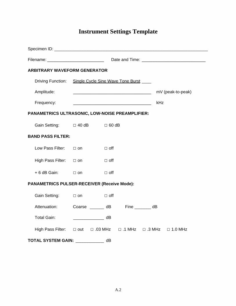
Instrument Settings Template

Specimen ID: _________________________________________________________________ Filename: ________________________ Date and Time: ___________________________ ARBITRARY WAVEFORM GENERATOR Driving Function: Single Cycle Sine Wave Tone Burst ____ Amplitude: _________________________________ mV (peak-to-peak) Frequency: _________________________________ kHz PANAMETRICS ULTRASONIC, LOW-NOISE PREAMPLIFIER: Gain Setting: □ 40 dB □ 60 dB BAND PASS FILTER: Low Pass Filter: □ on □ off High Pass Filter: □ on □ off + 6 dB Gain: □ on □ off PANAMETRICS PULSER-RECEIVER (Receive Mode): Gain Setting: □ on □ off Attenuation: Coarse ______ dB Fine _______ dB Total Gain: _____________ dB High Pass Filter: □ out □ .03 MHz □ .1 MHz □ .3 MHz □ 1.0 MHz TOTAL SYSTEM GAIN: ____________ dB

A.2

Scan Plan Template

Filename: ________________________ Date and Time: ___________________________ Listing of Inspection Personnel: Name: Title: Organization: ____________________________ ____________________ _________________________ ____________________________ ____________________ _________________________ ____________________________ ____________________ _________________________ SAFT-UT Parameter Header File (attached) □ Search Unit Type: Focused □ Flat □ Dual Element □ Search Unit Size:______________ Frequency of Inspection (kHz) 200 □ 250 □ 300 □ 350 □ 400 □ 450 □ Type of Scan: Pulse-echo □ Pitch-catch □ Beam Angle (incident angle in degrees): 0 □ 30 □ 45 □ 60 □ Beam Direction with Respect to Weld and Flow Direction: see component information attachment Acoustic Mode of Inspection: Longitudinal □ Shear □ Surface Wave □ Area and Volume of Component to be Examined:____________________________________________ ___________________________________________________________________________________ ___________________________________________________________________________________ ___________________________________________________________________________________ Flaw Types and Orientation to be Detected: ________________________________________________ ___________________________________________________________________________________ ___________________________________________________________________________________ Notes: ___________________________________________________________________________________ ___________________________________________________________________________________ ___________________________________________________________________________________ ___________________________________________________________________________________ ___________________________________________________________________________________

A.3

Component Information Filename: ________________________ Date and Time: ___________________________ Component Description: ______________________________________________________ ___________________________________________________________________________ ___________________________________________________________________________ Component Identification (if applicable): ___________________________________________ Description of Microstructure: ___________________________________________________ ___________________________________________________________________________ Average Grain Diameter: ____________ Component OD: ___________________ Component Drawing*: *Note: indicate flow and beam direction with respect to weld in the drawing below.

A.4

Component Information (continued)

SCAN PLAN VIEW GRID

A.5

A.6

Calibration Template Filename: ________________________ Date and Time: ___________________________ Header File (attached) □ Reference Sensitivity: _________________________________________________________________ Instrument Settings (see attachment) □ Scan Plan (see attachment) □ Component Information (see attachment) □

Appendix B

Discussion of Specimens

Specimen A Analysis

B.1

B.2

B.3

B.4

Specimen B Analysis

B.5

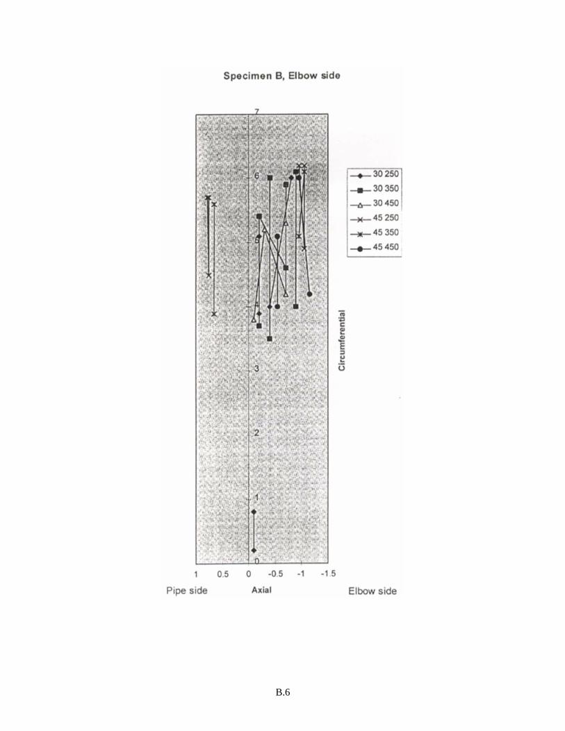
B.6

B.7

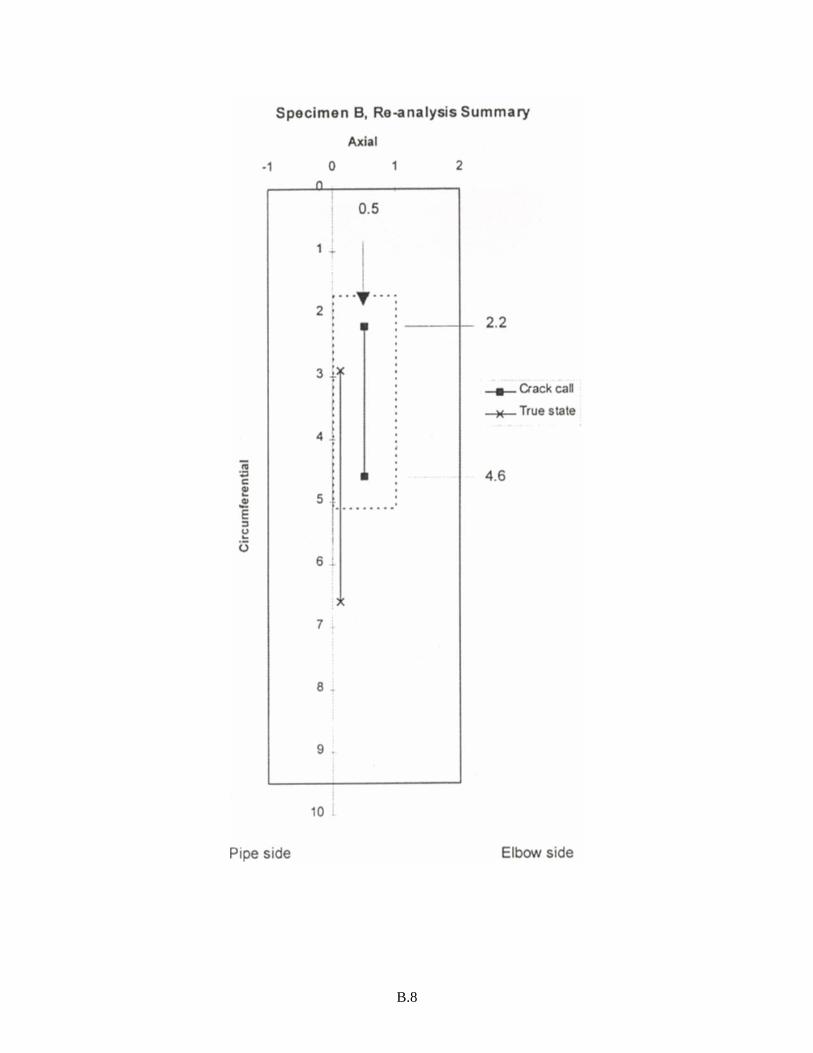
B.8

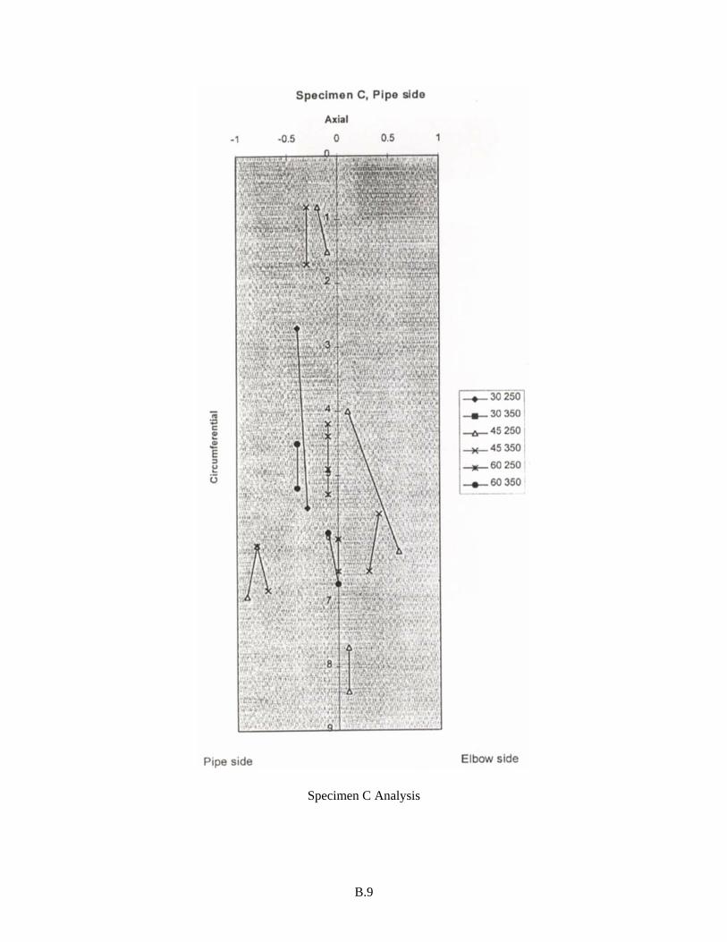
Specimen C Analysis

B.9

B.10

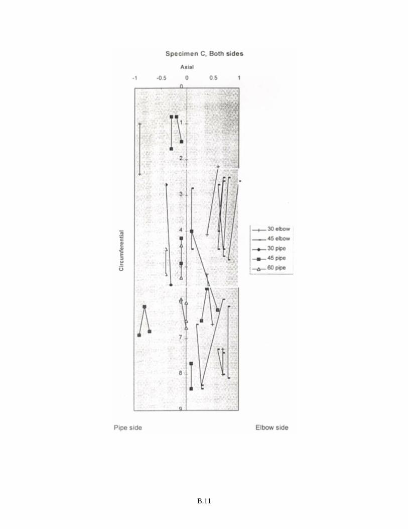
B.11

B.12

Specimen D Analysis

B.13

B.14

B.15

B.16

Specimen E Analysis

B.17

B.18

B.19

B.20

B.21

B.22

Specimen F Analysis

B.23

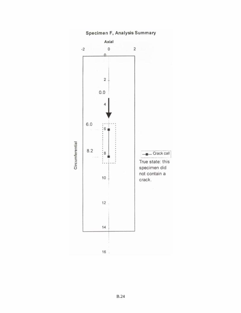
B.24

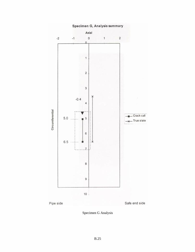
Specimen G Analysis

B.25

B.26

Appendix C

Step-by-Step Various Stages of Analysis Using the SAFT-Processed Ultrasonic Images

Figure C1 C-scan View of Specimen “B”, 30° Incident Angle, 250 kHz from the Pipe Side

C.1

Figure C2 C-scan View of Specimen “B”, 30° Incident Angle, 350 kHz from the Pipe Side –3 dB Clip

C.2

Figure C3 C-scan View of Specimen “B”, 45° Incident Angle, 350 kHz from the Pipe Side –3 dB Clip

C.3

Figure C4 C-scan View of Specimen “B”, 60° Incident Angle, 350 kHz from the Pipe Side –3 dB Clip

C.4

Figure C5 C-scan View of Specimen “B”, 30° Incident Angle, 350 kHz from the Elbow Side using A-scan Subtraction Algorithm

C.5

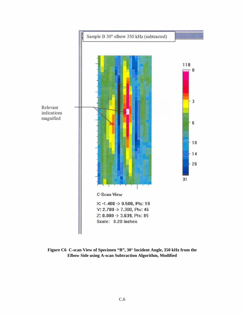
Figure C6 C-scan View of Specimen “B”, 30° Incident Angle, 350 kHz from the Elbow Side using A-scan Subtraction Algorithm, Modified

C.6

Figure C7 C-scan View of Specimen “B”, 30° Incident Angle, 350 kHz from the Elbow Side

C.7

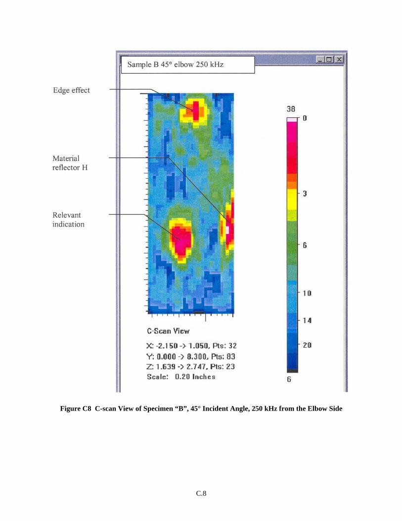
Figure C8 C-scan View of Specimen “B”, 45° Incident Angle, 250 kHz from the Elbow Side

C.8

Figure C9 C-scan View of Specimen “B”, 45° Incident Angle, 250 kHz from the Elbow Side using A-scan Subtraction Algorithm

C.9

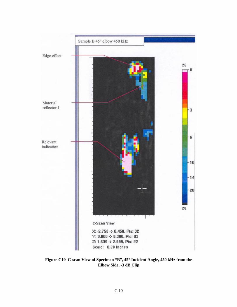
C.10

Figure C10 C-scan View of Specimen “B”, 45° Incident Angle, 450 kHz from the Elbow Side, -3 dB Clip