Fibre Based Modeling of WoodDynamics and Fracture

by

Sean Meiji Sutherland

B.Sc., The University of British Columbia, 2008

A THESIS SUBMITTED IN PARTIAL FULFILLMENT OFTHE REQUIREMENTS FOR THE DEGREE OF

MASTER OF SCIENCE

in

The Faculty of Graduate Studies

(Computer Science)

THE UNIVERSITY OF BRITISH COLUMBIA

(Vancouver)

October 2012

c⃝ Sean Meiji Sutherland 2012

Abstract

We present a model for the simulation of the dynamics and fracturing char-acteristics of wood, specifically its anisotropic behaviour. Existing workfocuses on FEM or other uniform lattice representations, with anisotropybeing modeled by data driven parameters. Our model instead utilizes anunderlying structure that is inherently anisotropic. We utilize an existingdescription of thin discrete elastic rods to build a fibrous material, ultimatelyyielding the characteristic splintering behaviour of wood. Our model extendsupon the existing work by defining coupling forces between these discreterods, allowing the construction of cohesive bundles of fibres. Additionally,we describe the conditions under which fracture occurs in the material. Therod and coupling components in the model are handled separately, as in thedynamics, resulting in inherently anisotropic responses. We conclude witha brief validation, followed by a discussion of possible future work.

ii

Table of Contents

Abstract . . . . . . . . . . . . . . . . . . . . . . . . . . . . . . . . . ii

Table of Contents . . . . . . . . . . . . . . . . . . . . . . . . . . . . iii

List of Figures . . . . . . . . . . . . . . . . . . . . . . . . . . . . . . v

1 Introduction . . . . . . . . . . . . . . . . . . . . . . . . . . . . . 11.1 Problem . . . . . . . . . . . . . . . . . . . . . . . . . . . . . 11.2 Overview . . . . . . . . . . . . . . . . . . . . . . . . . . . . . 2

2 Related Work . . . . . . . . . . . . . . . . . . . . . . . . . . . . 32.1 Concrete Models . . . . . . . . . . . . . . . . . . . . . . . . . 32.2 Wood Models . . . . . . . . . . . . . . . . . . . . . . . . . . 32.3 Fibre-based Models . . . . . . . . . . . . . . . . . . . . . . . 4

3 Wood Mechanics Model . . . . . . . . . . . . . . . . . . . . . . 53.1 Motivation . . . . . . . . . . . . . . . . . . . . . . . . . . . . 53.2 Discrete Elastic Rods . . . . . . . . . . . . . . . . . . . . . . 5

3.2.1 Discrete Rod Representation . . . . . . . . . . . . . . 63.2.2 Rod Bending . . . . . . . . . . . . . . . . . . . . . . . 73.2.3 Rod Stretching . . . . . . . . . . . . . . . . . . . . . . 83.2.4 Material Frame . . . . . . . . . . . . . . . . . . . . . 93.2.5 Collisions . . . . . . . . . . . . . . . . . . . . . . . . . 9

3.3 Wood Model Structure . . . . . . . . . . . . . . . . . . . . . 103.3.1 Rod placement . . . . . . . . . . . . . . . . . . . . . . 103.3.2 Binding Forces . . . . . . . . . . . . . . . . . . . . . . 11

3.4 Fracture Model . . . . . . . . . . . . . . . . . . . . . . . . . . 143.4.1 Single Rod Fracture . . . . . . . . . . . . . . . . . . . 153.4.2 Inter-rod Fracture . . . . . . . . . . . . . . . . . . . . 16

iii

Table of Contents

4 Validation and Observations . . . . . . . . . . . . . . . . . . . 174.1 Energy Conservation . . . . . . . . . . . . . . . . . . . . . . 174.2 Observations . . . . . . . . . . . . . . . . . . . . . . . . . . . 194.3 Implementation Details . . . . . . . . . . . . . . . . . . . . . 19

5 Rendering . . . . . . . . . . . . . . . . . . . . . . . . . . . . . . 205.1 Mesh Initialization . . . . . . . . . . . . . . . . . . . . . . . . 20

5.1.1 Cross Sectional Mesh . . . . . . . . . . . . . . . . . . 205.1.2 Mesh Extrusion . . . . . . . . . . . . . . . . . . . . . 21

5.2 Mesh Alignment . . . . . . . . . . . . . . . . . . . . . . . . . 225.3 Handling Fracture Events . . . . . . . . . . . . . . . . . . . . 24

5.3.1 Single Rod Fracture . . . . . . . . . . . . . . . . . . . 245.3.2 Inter-rod Fracture . . . . . . . . . . . . . . . . . . . . 26

6 Future Work and Improvements . . . . . . . . . . . . . . . . 276.1 Twisting Mechanics . . . . . . . . . . . . . . . . . . . . . . . 276.2 Fracture Conditions . . . . . . . . . . . . . . . . . . . . . . . 276.3 Constraints . . . . . . . . . . . . . . . . . . . . . . . . . . . . 286.4 Rod Collisions . . . . . . . . . . . . . . . . . . . . . . . . . . 29

7 Conclusion . . . . . . . . . . . . . . . . . . . . . . . . . . . . . . 30

Bibliography . . . . . . . . . . . . . . . . . . . . . . . . . . . . . . . 31

iv

List of Figures

3.1 Wood Cells and Fracture Photos . . . . . . . . . . . . . . . . 63.2 One Dimensional Rod Representation . . . . . . . . . . . . . 73.3 Rod Placement Diagram . . . . . . . . . . . . . . . . . . . . . 103.4 Rod Coupling Definition and Representation . . . . . . . . . 123.5 Rod Fracture Conditions and Treatment . . . . . . . . . . . . 14

4.1 Energy Conservation Example . . . . . . . . . . . . . . . . . . 184.2 Snapshots of Splintering Simulation . . . . . . . . . . . . . . 18

5.1 Mesh Initialization . . . . . . . . . . . . . . . . . . . . . . . . 215.2 Mesh Alignment and Fracture Handling . . . . . . . . . . . . 235.3 Rendering Mesh Demonstration . . . . . . . . . . . . . . . . . 26

v

Chapter 1

Introduction

1.1 Problem

The problem of modeling material fracture is an area well studied in com-puter graphics and physically-based animation [12]. While great advance-ments have been made, much of the research focuses around the simulationof isotropic materials. These include metals, ceramics, glass, and other ma-terials whose physical properties are largely independent of orientation.

While many objects that would be of interest to simulate are in fact madeof such isotropic materials, organic matter generally does not fall underthis category. In particular, wood exhibits highly anisotropic behaviour,especially with respect to fracturing.

This behaviour is caused by the internal structure of wood [20]. Woodis composed of straw-like cells, arranged in a parallel configuration. Be-cause the individual cells have directional structure, the overall material hasaccordingly anisotropic mechanics.

One approach to model such mechanics is to use a uniform materialbut with anisotropic response. Our research proposes a model for wooddynamics that will allow us to capture this anisotropy by instead simulatinga structure that inherently resembles that of the original material.

We use existing work on thin elastic rods to build a fibrous structureresembling that of wood. These rods are held together by binding forcesso that they can behave as one cohesive material. This approach allowsus to intuitively model the rods’ internal forces and external binding forcesseparately, and still achieve the desired anisotropic behaviour of the overallmaterial.

The same approach is taken for the fracture conditions of the wood.Since the rods themselves and the binding forces are already separate enti-ties, each can have separate fracture models. There is no need to force anyanisotropic behaviour onto these conditions, because the underlying struc-ture will induce anisotropic fracture patterns inherently.

1

1.2. Overview

1.2 Overview

This thesis consists of 5 chapters following this introduction. In Chapter2, we discuss related work in the field. Chapter 3 contains the details ofour wood model, and consists of 4 major sections. The first is a descriptionof the motivation behind our model, followed by an outline of the discreteelastic rod work by Bergou et al. [1] that forms the basis for our woodstructure. The last two sections discuss our treatment of the rod bindingforces, and of the fracture conditions for our model. In Chapter 4, we discussthe testing and results of our model. Chapter 5 describes the constructionof a triangle mesh that can be used in rendering our wood model, followedby a conclusion in Chapter 6.

2

Chapter 2

Related Work

There has been extensive work done in modeling the dynamics of homo-geneous and isotropic materials. Research in modeling materials that areinhomogeneous or anisotropic is not as prevalent, with the majority of thework being heavily driven by experimental data. This is due to the fact thatthe work often focuses on building materials such as wood or concrete, andis intended for engineering applications. In applications where the toleranceof a material to fracture is being simulated for engineering purposes, themodel must have a high degree of accuracy, which often requires the modelto be data driven.

2.1 Concrete Models

Much of the work in the modeling of inhomogeneous materials is focused onsimulating concrete[18]. Generally concrete is composed of sand, gravel, andstone embedded in cement, and this inhomogeneity gives concrete its uniquephysical properties. In simulation, the material is frequently modeled usinga finite element method (FEM)[7, 11]. Finite element methods are a robustrepresentation that allows the model to be driven by experimental data,which, as mentioned above, is common in the modeling of these materials.The use of such a method also allows inhomogeneity to be built into thesystem intuitively. The separate components of the concrete can simply berepresented with different element parameters. For example, Schlangen andGarboczi [15] employ a lattice model, in which vertices and their connectionsare modeled as separate entities, with corresponding dynamics and equationsof motion.

2.2 Wood Models

In addition to inhomogeneous materials, the modeling of materials that ex-hibit anisotropic response is also well studied. Among such materials, acommon area of interest is the modeling of wood behaviour. Like concrete,

3

2.3. Fibre-based Models

much of the work is based around FEMs [5, 6]. FEM models use a represen-tation that is uniform across the entire model, and anisotropy is achievedthrough varying the parameters controlling inter-element interaction basedon direction. Often these parameters are obtained through experimentaldata [16, 19], and the work has been extended to the use of non-standard fi-nite element formulations [13, 17]. In contrast to this work, our model strivesto build a structure using a representation that is inherently anisotropic, atopic briefly mentioned in Vasic, Smith, and Landis [21]. We utilize existingwork in modeling thin fibre dynamics[1, 8] as a basis for our model.

2.3 Fibre-based Models

Many real world materials have a fibrous structure, such as wood, rope, andhair. Hair modeling can be of particular interest. Physically implausible hairmovement is very noticeable to the human eye, and the level of detail re-quired can be very expensive [24]. Many different representation techniquesexist for modeling hair, such as mass spring systems [14], rigid body chains[9], and super helices [2, 10]. The work has been extended to methods fordynamically grouping strands of hair for more efficient and realistic results[3, 22]. In more abstract fibre modeling, Bergou et al. [1] define a settingfor thin elastic rods with small cross section. Our model heavily utilizes thiswork as a basis for our fibrous wood structure.

4

Chapter 3

Wood Mechanics Model

We develop a physical model for wood mechanics that inherently capturesthe fibrous nature of the material. We draw upon the discrete elastic rodmodel described by Bergou et al. [1] as an underlying component in ourdescription. These rods are bound together by forces designed to opposerelative translational movement. Finally, we implement conditions for thefracturing of our material.

This chapter will describe the motivation behind our model, followed bythe details of each component therein.

3.1 Motivation

Wood is a naturally fibrous material, the bulk of which is made up of millionsof straw-like wood cells, as can be seen in Figure 3.1(a). This structure leadsto a lot of the characteristic behaviour we observe in wood. In particular,it gives rise to the splintering effect we see when wood is broken, as shownin Figure 3.1(b). While the splintered pieces are of a vastly different scalethan the wood cells themselves, the anisotropy in the fracture patterns islargely caused by that of the underlying structure.

Anisotropy is also introduced by having the types of wood cells veryacross the material, in other words the “grain” of the wood. While we donot incorporate any notion of grain in our model, it is certainly a strongconsideration for future work.

It is not computationally feasible at present to dynamically simulatestructure on the order of individual wood cells. However, it is possiblefor the model to capture the characteristic fracture behaviour even with arelatively coarse fibre-like representation.

3.2 Discrete Elastic Rods

The first step in defining our structure is to create a model of an individualfibre. We use the discrete elastic rod model described by Bergou et al.[1],

5

3.2. Discrete Elastic Rods

Figure 3.1: (a) An image of microscopic wood cell structure. Image courtesyof Ian Smith [16] (b) A photograph illustrating the characteristic splinteringbehaviour of wood fracture. Image courtesy of Gene Wengert [23]

based on Kirchhoff’s theory of elastic rod mechanics. In this work, rodsare described by their centerline curve, and the material frame coordinatesalong that curve. They are assumed to have a constant cross-section that issmall in comparison to the length of the rod.

Here we will give a brief description of the equations of motion for theserods that are pertinent to our wood model. An in depth discussion of thederivation and physics behind the equations can be found in the originalpaper[1]. While these rods can have arbitrary undeformed configurations,our model only uses straight rods, and therefore that will be the assumptionthroughout this section.

3.2.1 Discrete Rod Representation

The state of a one dimensional continuous rod can be described by Γ ={γ; t,m1,m2}. Here γ(s) represents the rod’s arclength parameterized cen-terline, and {t(s),m1(s),m2(s)} describe the orthonormal material frame ateach point along the rod (see Figure 3.2). This material frame is constrainedby the property that t(s) = γ′(s), to ensure that one axis lies tangent to thecenterline curve.

In the discretized case, we replace the centerline, γ(s) with verticesx0, . . . , xn. These vertices are connected by edges, which we refer to ase0, . . . , en−1, with ei = xi+1 − xi. These edges are the discretization ofthe tangent component t(s) of the material frame above. Each vertex alsohas associated with it vectors representing the other two components of thematerial frame.

6

3.2. Discrete Elastic Rods

Figure 3.2: The continuous and discrete representations of a one dimensionalrod.

Rod vertices also have mass values associated with them. We assumeuniform mass distribution along the rod, so the mass of each vertex is basedon its surrounding edge lengths. In particular, the mass at vertex xi isproportional to ∥ei−1∥ + ∥ei∥, with the appropriate term excluded for x0and xn.

The forces governing these rods consist of two components, bending andstretching. Our model does not incorporate any force resisting the twist ofa single rod. In both cases, we describe the potential energy of the systemresulting from such deformations, followed by the induced force. We firstlook at the bending energy of a discrete rod.

3.2.2 Rod Bending

According to Kirchhoff’s model, the bending energy of a rod takes the form

Ebend =1

2

∫α∥κ∥2ds (3.1)

where α is the rod’s bending modulus and κ is the curvature of the rod. Thisenergy has the physical interpretation of being based on the stretching andcompressing of the outer and inner part of a curved rod. This lends itselfto the rod fracture conditions described later. Bergou et al. show in theirpaper that the analysis of the geometry of a discrete rod naturally yieldsthe following form for the curvature at xi[1]:

κi = 2 tanϕi

2(3.2)

with ϕi as defined in Figure3.2. Using this, we can then define the curva-ture binormal as the vector having magnitude κi = 2 tan(ϕi/2) and beingorthogonal to the edges adjacent to xi:

7

3.2. Discrete Elastic Rods

κbi =2ei−1 × ei

∥ei−1∥∥ei∥+ ei−1 · ei(3.3)

where ∥ei∥ denotes the rest length of edge ei.When we express the bending energy above in terms of the corresponding

discrete quantities, we get

Ebend =1

2

∑α

(κbili/2

)2li2=∑ α(κbi)

2

li(3.4)

where li = ∥ei−1∥ + ∥ei∥, accounting for the measure of the domain in theintegral.

In order to find the forces acting upon the vertices due to bending defor-mation, we take the gradient of this energy. Since the curvature binormalonly depends on adjacent edges, and therefore on the adjacent vertices, thegradient term for a vertex xi will only depend on the information at xi, xi−1,and xi+1, when they exist. The force on xi can therefore be expressed as asum of up to 3 terms of the form

−2α

lj(▽i(κ

b)j)T (κb)j (3.5)

where i− 1 ≤ j ≤ i+ 1. The gradient of the curvature binormal is given bythe following expressions

▽i−1κbi =

2[ei] + (κbi)(ei)T

∥ei−1∥∥ei∥+ ei−1 · ei(3.6)

▽i+1κbi =

2[ei−1]− (κbi)(ei−1)T

∥ei−1∥∥ei∥+ ei−1 · ei(3.7)

▽iκbi = −(▽i−1 +▽i+1)(κ

bi) (3.8)

where [e] is the skew symmetric 3x3 matrix satisfying [e]x = e × x for any3-vector x.

3.2.3 Rod Stretching

For the stretching component of the rod’s energy, we use a simple springmodel

Estretch =1

2

n−1∑i=0

k(∥xi+1 − xi∥/∥ei∥ − 1)2∥ei∥ (3.9)

8

3.2. Discrete Elastic Rods

where k is the rod’s spring constant. After taking the gradient, we find theforce on a vertex xi to be given by

Fstretch = −k

[(∥xi+1 − xi∥∥ei∥

− 1

)xi+1 − xi

∥xi+1 − xi∥

+

(∥xi − xi−1∥∥ei − 1∥

− 1

)xi − xi−1

∥xi − xi−1∥

](3.10)

3.2.4 Material Frame

The material frame represents the orientation of material at each vertexpoint. As mentioned earlier, the t direction is constrained to be along theedge of the rod. The m1 and m2 directions represent the twist of the rod.As our model does not incorporate a twist force, the only use of these axesof the material frame is for rendering purposes, described later.

At the initialization of a rod, the orientation of the twist axes of thematerial frame is arbitrary, though the same for all vertices. At each timestep, and for each vertex xi, consider the edges e

t−1i and eti with superscripts

denoting the time step. Let ρi = cos−1(et−1i · eti/(∥e

t−1i ∥ · ∥eti∥)) be the angle

of the rotation of the edge during the time step, and hi = et−1i × eti the axis

of the rotation. Each of the material frame axes of xi from the previousstate are rotated by ρi about the vector hi to form the new material frame.

3.2.5 Collisions

Our model does not incorporate any detection or resolution of collisionsbetween two rods or rods with itself. The only such interactions our modelhandles are those provided by the binding forces of our wood model describedin the next section. The potential use of such collision detection is discussedin Section 6.4.

We do, however, model the interactions between rods and external rigidbodies. We use the assumption that the bodies are large relative to the edgelengths of rods, so that we need only to check the intersection of rigid bodieswith individual rod vertices.

Each rod vertex is tested as to whether it is inside a rigid body. If anintersection is found, then the positions of the rigid body and the vertexare adjusted as if they had undergone a perfectly elastic collision, giventheir mass and current velocity. If a collision is resolved, all other intersec-tions are rechecked until no collisions are found, up to a given threshold ofinteractions.

9

3.3. Wood Model Structure

Figure 3.3: This figure illustrates the process by which rods are placed withina cylindrical wood structure. First, 2D points are sampled within a circularboundary. These points are then extruded in the third dimension to yieldrods.

3.3 Wood Model Structure

Using the discrete rods described above, our wood model can now be built.We use the strand like nature of the rods to macroscopically emulate thebundles of fibres that yield the characteristic behaviour of wood. In thefollow sections, we describe the method by which we use these rods to con-struct our model. We discuss the inter-rod behaviour that we desire andconstruct the corresponding potential functions, as well as the forces thatare derived as a result.

3.3.1 Rod placement

Our structure is built using a set of rods placed within some bound, sep-arated by some minimum distance. For simplicity, we modeled the woodas having an approximately cylindrical boundary. We also restricted therods to being parallel to the axis of the cylinder. This simplifies the rodplacement algorithm to be generating points within the 2D cross section ofthe wood, and then extruding these points into rods. The rod placement isrestricted so that no two rods are within some given minimum distance, µ,of each other.

First, points are sampled within a 2D circle, corresponding to the crosssection of the wood, as shown in Figure 3.3. The process for this is comprisedof two separate parts, both making use of a Poisson disk sampling method[4]. We first use a simplified 1D implementation of the algorithm to samplepoints in [0, 2π], and use these to generate points around the edge of the

10

3.3. Wood Model Structure

cross section. Then, points are sampled within the cross section using a 2Dimplementation of the same algorithm.

In sampling the points from [0, 2π], we first generate a starting point,p0, sampled uniformly in [0, µ]. We then repeat the process of taking themost recently placed point, p, and uniformly sampling a new point in therange [p+µ, p+2µ]. This process is stopped when a point is sampled withindistance µ of 2π + p0 or is greater than 2π. These two conditions togetherare equivalent to stopping when a point is sampled with distance µ of p0,if we interpret the boundaries of our space as being periodic. We then takethese sampled points as angles for rod placement along the edge of the woodcross section.

Next, we sample points within the interior of the wood cross section. Wedefine a set of points, S, and a set of “active” point, A, both initialized tothe set of points along the cross section edge created above. The followingsteps are repeated until A is empty. Step 1: take an arbitrary point p ∈ A.Step 2: uniformly sample (r, θ) from [µ, 2µ]× [0, 2π], and consider the pointx when (r, θ) are interpreted as polar coordinates centered on p. Point xis considered valid if it is at least distance µ from every point in S, and iscontained within the wood cross section. Step 3: If x is not valid, then repeatstep 2. This process will repeat a fixed number of times, the limit being atuneable parameter. If no valid point is found within these iterations, p isremoved from A, and the algorithm repeats from Step 1. If x is valid it isadded to both A and S, p is removed from A, and the algorithm repeatsfrom Step 1.

The set of points S generated by this algorithm are the points that willbe extruded along the length of the wood to form rods, as demonstratedin Figure 3.3. In our model, the rods generated are always parallel andspan the entire cylindrical region of the wood. The locations of internalvertices for each rod, however, are randomly generated with some thresholdsfor minimum and maximum edge length. The random placement of rodvertices mitigates some aliasing effects in the simulation. The introductionof randomness at this level of the model leads to desirable noise in theeventual fracture pattern.

3.3.2 Binding Forces

The next step in building the wood structure is to determine which portionsof the wood are bound together. While a simple approach would be to createbinding constraints between vertices of nearby rods, the random nature ofthe placement of these vertices makes this often impractical. Frequently, a

11

3.3. Wood Model Structure

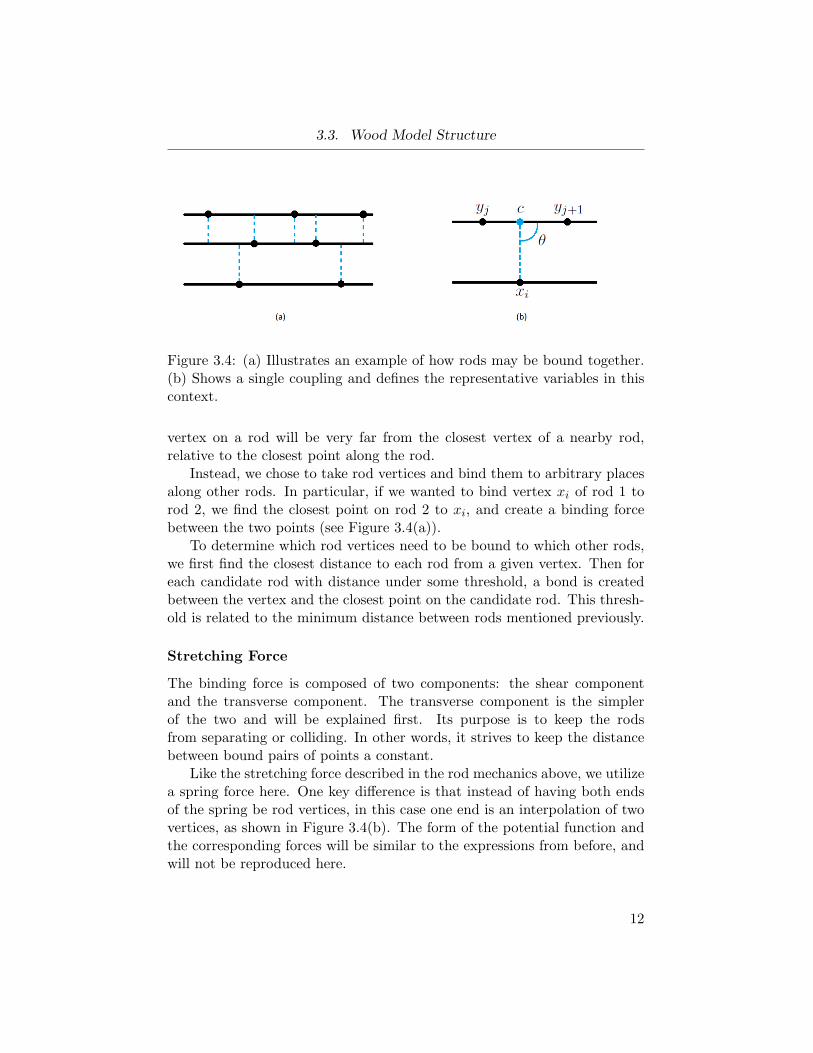
Figure 3.4: (a) Illustrates an example of how rods may be bound together.(b) Shows a single coupling and defines the representative variables in thiscontext.

vertex on a rod will be very far from the closest vertex of a nearby rod,relative to the closest point along the rod.

Instead, we chose to take rod vertices and bind them to arbitrary placesalong other rods. In particular, if we wanted to bind vertex xi of rod 1 torod 2, we find the closest point on rod 2 to xi, and create a binding forcebetween the two points (see Figure 3.4(a)).

To determine which rod vertices need to be bound to which other rods,we first find the closest distance to each rod from a given vertex. Then foreach candidate rod with distance under some threshold, a bond is createdbetween the vertex and the closest point on the candidate rod. This thresh-old is related to the minimum distance between rods mentioned previously.

Stretching Force

The binding force is composed of two components: the shear componentand the transverse component. The transverse component is the simplerof the two and will be explained first. Its purpose is to keep the rodsfrom separating or colliding. In other words, it strives to keep the distancebetween bound pairs of points a constant.

Like the stretching force described in the rod mechanics above, we utilizea spring force here. One key difference is that instead of having both endsof the spring be rod vertices, in this case one end is an interpolation of twovertices, as shown in Figure 3.4(b). The form of the potential function andthe corresponding forces will be similar to the expressions from before, andwill not be reproduced here.

12

3.3. Wood Model Structure

Shear Force

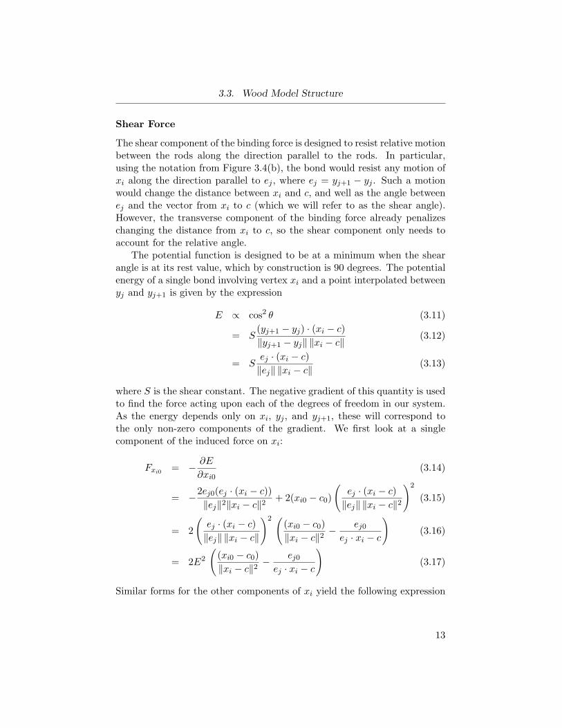
The shear component of the binding force is designed to resist relative motionbetween the rods along the direction parallel to the rods. In particular,using the notation from Figure 3.4(b), the bond would resist any motion ofxi along the direction parallel to ej , where ej = yj+1 − yj . Such a motionwould change the distance between xi and c, and well as the angle betweenej and the vector from xi to c (which we will refer to as the shear angle).However, the transverse component of the binding force already penalizeschanging the distance from xi to c, so the shear component only needs toaccount for the relative angle.

The potential function is designed to be at a minimum when the shearangle is at its rest value, which by construction is 90 degrees. The potentialenergy of a single bond involving vertex xi and a point interpolated betweenyj and yj+1 is given by the expression

E ∝ cos2 θ (3.11)

= S(yj+1 − yj) · (xi − c)

∥yj+1 − yj∥ ∥xi − c∥(3.12)

= Sej · (xi − c)

∥ej∥ ∥xi − c∥(3.13)

where S is the shear constant. The negative gradient of this quantity is usedto find the force acting upon each of the degrees of freedom in our system.As the energy depends only on xi, yj , and yj+1, these will correspond tothe only non-zero components of the gradient. We first look at a singlecomponent of the induced force on xi:

Fxi0 = − ∂E

∂xi0(3.14)

= −2ej0(ej · (xi − c))

∥ej∥2∥xi − c∥2+ 2(xi0 − c0)

(ej · (xi − c)

∥ej∥ ∥xi − c∥2

)2

(3.15)

= 2

(ej · (xi − c)

∥ej∥ ∥xi − c∥

)2 ((xi0 − c0)

∥xi − c∥2− ej0

ej · xi − c

)(3.16)

= 2E2

((xi0 − c0)

∥xi − c∥2− ej0

ej · xi − c

)(3.17)

Similar forms for the other components of xi yield the following expression

13

3.4. Fracture Model

Figure 3.5: (a) A diagram of the relevant variables when considering thebending stress at a rod vertex. (b) Illustrates the result of a rod fractureoccurring.

for the force on xi

Fxi = 2E2

((xi − c)

∥xi − c∥2− ej

ej · xi − c

)(3.18)

Likewise, the forces upon yj and yj+1 are given by the expressions

Fyj =2(ej · (xi − c))(xi0 − c0)

∥xi − c∥2∥ej∥− 2ej

(ej · (xi − c)

∥ej∥ ∥xi − c∥2

)2

(3.19)

= 2E2

(xi − c

ej · (xi − c)− ej

∥ej∥2

)(3.20)

(3.21)

Fyj+1 = 2E2

(ej

∥ej∥2− xi − c

ej · (xi − c)

)(3.22)

= −Fyj (3.23)

3.4 Fracture Model

The final step in building our wood model is to define the condition underwhich the material undergoes fracture. Our model conceptually separatesthe nature of forces within rods from those between rods, in order to incor-porate an inherent anisotropic nature. Thus it follows that separate fractureconditions should be created to deal with stresses within a rod, and stresseson the binding forces between them.

14

3.4. Fracture Model

3.4.1 Single Rod Fracture

The fracture conditions for a single rod are based on a combination of thestresses within that rod. The discrete elastic rod model we use has bendingand stretching stress energies, and therefore these are the deformations thatthe fracture condition will depend on.

The stresses within a rod are evaluated at each of the interior vertices,and consist of two components: stretching and bending. In both cases, thefracture condition is based on the ratio of the length between the deformedmaterial, and the rest state. This representation will later allow us to easilycombine the two terms into a single value.

While the amount of stretching on a rod is something more naturallyassociated with its edges, for the purposes of evaluating fracture it is con-venient to have both of the fracture conditions associated with the samecomponents of the model, in this case the vertices. As a result, we simplyaverage the deformation ratios for each of the vertex’s neighbouring edgesto achieve our result.

For computing the deformation ratio due to bending, we consider therelative length of the outer edge of the rod to the centerline. Because thediscrete representation does not give us a curved centerline, we interpolateone near the vertex in question (see Figure 3.5a). We first find the circlethat interpolates the vertex, xi, and its two neighbours, which lies in theplane defined by those vertices. The arc of this circle within the solid angleformed by xi−1, xi+1 and C (the circle center) are what we will use as ourreference length.

We then construct a second concentric circle with the radius increasedby half of the cross-sectional radius of the rod. The length of this circle’sarc with the same solid angle will be the deformed outer edge length. Wedivide these two length to compute the bending deformation ratio.

Rθ

rθ=

r + 12h

r= 1 +

h

2r= 1 +

h

2∥xi − C∥(3.24)

where r and R are the radii of the inner and outer circle respectively, h isthe cross-sectional radius of the rod, and C the center of the circles.

At each vertex we can now evaluate both the length ratios due to stretch-ing and bending, and multiply them to obtain a total deformation ratio.When this value passes some predetermined threshold, the rod is brokenat that point. We replace a rod consisting of vertices x0, . . . , xn, fracturedat xf , with two new rods y0, . . . , yf and z0, . . . , zn−f with vertex locationsat x0, . . . , xf and xf , . . . , xn respectively (Figure 3.5b). All of the binding

15

3.4. Fracture Model

forces between the rods are also updated to reference the corresponding ver-tices from the new rods. Any forces tied to xf are duplicated for yf and z0.Bonds to edge ef−1 are assigned to the edge between yf−1 and yf . Similarly,bonds to edge ef are assigned to z0 and z1.

3.4.2 Inter-rod Fracture

The condition for breaking the inter-rod binding forces is simpler than fora single rod. For each binding force in the wood, we evaluate the sum ofthe shear and transverse potential. As above, if the value crosses somepredetermined threshold, the bond is removed. A weighted mean of the twocomponents can be used instead, with the weight left as a parameter.

16

Chapter 4

Validation and Observations

4.1 Energy Conservation

As our work is a simulation of a physical system, we want the total energy ofour system to remain as constant as possible. The result of a fracture eventoccurring is a decrease in the energy of our system as we have defined it,consisting only of potential and kinetic energy. In reality, a fracture eventwould convert much of the potential energy to forms other than kinetic, suchas sound or heat.

However, it is still desirable that the other aspects of the system, specifi-cally those concerned with forces acting upon the degrees of freedom, respectthe conservation of energy. The two determining factors of the energy sta-bility of the simulation are the equations governing the forces in our system,and the numerical integration method used to compute discretized motionfrom these forces.

All of the forces used in our system are derived from corresponding po-tential energy functions. This ensures that, at least in a continuous setting,these forces would yield motion that conserves the sum of potential and ki-netic energy, the only forms present in our model. The equations of motionare integrated using the Symplectic, or semi-implicit, Euler method. Theenergy of the system is quite close to being perfectly conserved using thistechnique.

To verify this conservation of energy, an experiment was set up using asection of wood. The initial state of the wood is set to be a bent configura-tion, with the rest state being straight, yielding an oscillating motion. Frac-ture events are disabled for this simulation, so that the conserving propertiesof the equations of motion can be observed alone. The results are shown inFigure 4.1.

17

4.1. Energy Conservation

Figure 4.1: The graph represents the sum of the potential and kinetic energyof the system. Snapshots indicate the oscillation occurring in the material.

Figure 4.2: Snapshots from three simulations illustrating splintering be-haviour.

18

4.2. Observations

4.2 Observations

In computer graphics, there is often no concrete metric by which to evaluatethe quality of a particular animation or model. Certainly there are specificdesirable properties, such as the conservation of energy as discussed above.In some cases, a high degree of physical accuracy is also required. In others,the goal is to create a model that captures the essential behaviour of somephenomenon, rather that to create an exact physical duplication.

Our model for wood behaviour is intended to fall into the latter category.As such, the primary method for evaluating the results is to visually identifythe desired behavioural characteristics. In Figure 4.2, we show snapshots ofa simulation intended to demonstrate splintering behaviour.

In this simulation, three blocks impart force upon a section of wood, andthe resulting stresses induce fracturing. The spatial scale of the model isintended to be on the order of a small branch, with the length of the rodsbeing 15cm. The time scale is approximately 3 seconds for each simulationshown.

4.3 Implementation Details

The simulation code was written in C++ and drew upon the Discrete Elas-tic Rods [1] project code generously provided by Miklos Bergou. At eachsimulation time step, the equations of motion are integrated using the Sym-plectic Euler method, with collisions between rods and rigid bodies thenbeing resolved afterwards.

Each of the simulations in Figure 4.2 had a run time of approximately1 hour for 3 seconds of simulation time. The run time could be dramati-cally improved through optimization techniques such as parallelization andgraphical hardware acceleration.

If the threshold distance for creating rod-rod bonds is linear in the min-imum distance of their placement (see Section 3.3.2) then the run timecomplexity in the number of rods is linear. This is because increasing thenumber of rods, and therefore their density, is equivalent to decreasing theminimum distance between them. This will result in each rod being boundto, on average, the same number of neighbouring rods. The per-rod dynam-ics computations are certainly linear in the number of rods, and with therod-rod bond dynamics being linear as well, this results in an overall linearcomplexity.

19

Chapter 5

Rendering

In this chapter we detail a method of creating a triangle mesh surroundingthe wood, for use in rendering. The mesh is designed with three importantproperties in mind. The first is that the mesh follows the rods throughoutthe simulation. This is accomplished by using coordinate systems that aretied to the rod state. The second requirement is that a portion of the meshsurrounding interconnected rods remains cohesive throughout simulation.During rendering, the mesh is dynamically adjusted to maintain this cohe-sion. The third property, crucial to the nature of the project as a whole, isthat the mesh easily accommodates fracture events during simulation. Thisis done inherently through the representation, which, as can be seen below,lends itself to both types of fracture present in our model.

5.1 Mesh Initialization

The rendering mesh is a set of triangle meshes covering each rod. The initialmesh is created using a two step process, similar to that of initializing therods themselves. The cross section of the rod bundle is used to create aVoronoi diagram, with each cell surrounding a single rod. These cells arethen extruded into meshes associated with each rod.

5.1.1 Cross Sectional Mesh

The first step is to define the boundaries between the rods, at least as faras the mesh is concerned. This will yield a cross sectional mesh from whichwe can extrude the rendering mesh. The cross sectional mesh is constructedusing a Voronoi diagram.

We first take the set of 2D points defining the cross section of the wood,as described in Section 3.3.1. The Voronoi diagram associates regions of theplane with the rod placement points. The boundaries between these regionswill become edges in our mesh, and the intersections of these boundaries willbecome vertices. These edges and vertices make up the base of our crosssectional mesh.

20

5.1. Mesh Initialization

Figure 5.1: (a) A cross sectional mesh, consisting of a Voronoi diagramwith a boundary. (b) Copies of a cross sectional polygon, aligned with rodvertices. (c) A pair of triangles constructed between two adjacent crosssectional polygons.

We bound the regions associated with the rods on the outer edge bycreating an extra boundary around the entire set of rods. For each rod witha non-bounded region, we create a vertex some fixed distance from the rodposition.

The vertices are placed radially outward relative the center of circle inwhich the rod positions were sampled. The fixed distance they are placedaway from the rod is equal to the minimum distance that was required whilesampling the rod positions.

Next, we take the convex hull of these new vertices, and add the resultingedges and vertices to the cross sectional mesh. This convex hull defines theouter edge, and as such, everything outside of it is discarded. We also insertnew vertices at any edge intersections. The final cross sectional mesh isshown in Figure 5.1(a).

5.1.2 Mesh Extrusion

The next step in creating the rendering mesh is to extrude the cross sectionalmesh into a 3D triangle mesh. Consider a single rod placement location inthe cross sectional mesh, and the polygon within which it is contained. Letus notate the rod point as x0, the polygon as P 0, and the vertices of P 0 asp01, p

02, . . . , p

0m.

During the initialization of the wood, the rod placement point x0 isextended to a full rod, with vertices x0, x1, . . . , xn. We create n additionalcopies of the polygon P 0, differentiated by superscript, with each translated

21

5.2. Mesh Alignment

a different length along the rod axis. Each copy of the polygon is alignedwith a rod vertex such that the polygon consisting of vertices pj1, p

j2, . . . , p

jm

is coplanar to xj , as shown in Figure 5.1(b).With our vertices in place, the triangles composing the rendering mesh

can be specified. We first specify quadrilaterals between these vertices. Aquadrilateral is created between points pji , p

j(i+1)mod m, pj+1

(i+1)mod m, pj+1i for

1 ≤ i ≤ m and 1 ≤ j ≤ n − 1. Next, these quadrilaterals are triangulated.The parity of the triangulation is arbitrary but kept consistent across theentire mesh. An example is shown in Figure 5.1(c). These triangles formthe first part of the rendering mesh.

To close the mesh, geometry must be added at both ends of the rods.The polygon p01, p

02, . . . , p

0m can be triangulated by having adjacent vertices

form a triangle with the rod point x0. A similar process can be repeated forthe other end of the rod. With these triangles included, the mesh is nowclosed.

The process of extruding a cross sectional mesh polygon into a full 3Dmesh is repeated for each rod. Note that many of the triangles in the interiorof the wood will not be initially visible. However creating these trianglesduring initialization will greatly simplify dealing with fracture events in thewood.

As the rod moves and deforms during simulation, the mesh must follow.In order to accomplish this, the mesh vertices must be stored as positionsrelative to the rod. The end points x0 and xn are already components ofthe rod state. The polygon pj1, p

j2, . . . , p

jm will have its vertices stored as

coordinates with respect to xj ’s material frame axes.

5.2 Mesh Alignment

With each rod having an entirely independent mesh, it is possible that visualartefacts will arise. The wood is intended to be a single solid object. As therods vertices move, however, the separate meshes may pull apart, giving theappearance of a hole in the mesh. This problem is solved by adjusting thelocations of the mesh vertices so that the boundaries between the adjacentrods meshes are as close to aligned as possible. For mesh edges and verticesto be considered adjacent, we also require the existence of a binding forcebetween the corresponding rods. This ensures that we only align portionsof the mesh that are connected in the context of the simulation.

After initialization of the rendering mesh, we find all the vertices thatlie on the edge or vertex of another rod’s mesh. Consider such a vertex, v,

22

5.2. Mesh Alignment

Figure 5.2: (a) An example of a mesh alignment iteration, with vertex-edgeassociations highlighted. (b) A single rod fracture event.

that lies on the edge, q, of another mesh, with q having vertices r and s.Let R1 be the rod associated the mesh that v belongs to, and R2 be that ofq. From the initialization, we know that each vertex of the mesh is part ofa cross sectional polygon associated with a single rod vertex. In addition,if a vertex were to lie on the edge of another mesh, that edge must spanvertices of two different cross sectional polygons. This is because the edgeswithin a cross sectional polygon line up precisely with those from adjacentmeshes, both being associated with a single edge of the Voronoi diagram.We further define xi to be the rod vertex corresponding to mesh vertex v,yj and yj+1 the rod vertices corresponding to mesh vertices r and s, andej the rod edge from yj to yj+1. If it is the case that a binding force wasconstructed between xi and a point along ej , we create what we call anassociation between v and q.

An association consists of v, r, s, and a scalar value λ parameterizingthe point along q coinciding with v. If we interpret the vertices as spatiallocations, λ satisfies v = (1 − λ)r + λs. In the case where v lies in thesame point as a vertex w of another mesh, only v and w are stored asan association. This process is repeated for all applicable vertices in therendering mesh. Note that an association of v with w is distinct from oneof w with v. A reference to the binding force we required is also stored inthe association.

During simulation, these associations can be used to adjust the mesh

23

5.3. Handling Fracture Events

vertices through an iterative procedure. We first outline a single iteration.Consider a vertex v with a single association, represented by r, s, and λ,as above. Let a = (1 − λ)r + λs, the point along the edge which initiallycoincided with v. We set the new position of v to be the midpoint between aand the current position of v. In the case that v is associated with a vertexw, the midpoint between v and w is instead used. In general it is possiblethat v will have two or more associations. In this situation the average of vand all associated points is used as the new position for v.

This adjustment is performed for every vertex in the mesh, and this setof adjustments comprises a single iteration of mesh alignment. An exampleof an alignment iteration is shown in Figure 5.2. Once the iterations of meshalignment are concluded, the mesh is ready to be rendered. The terminationcondition we use for alignment iterations is simply a fixed number of itera-tions. However, other conditions could be used, such as having an iterationwhere no vertex was adjusted by more than some threshold.

Note that the adjusted vertex locations are temporary, and the originalvertex location in the material frame coordinates of the rod are always keptintact. This is because the association may be removed during simulation, atwhich point the renderer reverts to the original vertex location. The adjustedlocation, transformed to material frame coordinates, can also be saved fromframe to frame. If a method with a variable number of iterations was used,this may increase efficiency. Even with a fixed number of iterations, a betteralignment can be found, as the deformation of the wood as compared to theprevious frame is frequently smaller than as compared to the initial state.

5.3 Handling Fracture Events

The rendering mesh was designed to easily handle fracture events duringsimulation. There are two types of fracture events. The first is a single rodbreaking into two pieces. The second is the binding force between two rodsbeing broken.

5.3.1 Single Rod Fracture

As described in Section 3.4.1, when a rod consisting of vertices x0, x1, . . . , xnundergoes a fracture event at vertex xf , two new rods are created withvertex locations at x0, . . . , xf and xf , . . . , xn. A similar process occurs forthe rendering mesh.

Let P j denote the cross sectional polygon of rod vertex xj . Let usfurther notate the two new rods as y and z, and their vertices y0, . . . , yf

24

5.3. Handling Fracture Events

and z0, . . . , zm, and Qj and Rk the cross sectional polygons of yj and zkrespectively. When a fracture event occurs at xf , first the cross sectionalpolygons are copied to the new rods. For all 0 ≤ j ≤ f , Qj will take on thecoordinates as P j . Similarly, for all 0 ≤ k ≤ m, Rk will have the coordinatesof P k+f . As the material frames of the new rod vertices correspond to thoseof the original rod, the material frame coordinates of the polygons do notneed to be transformed.

Triangles are then specified between vertices of adjacent cross sectionalpolygons. The parity of the triangulation should be consistent with that ofthe mesh of the original rod. The triangles closing the mesh at the rod endsare constructed by the same process as in the initialization. Polygon Q0 istriangulated using y0, along with Qf and yf , R

0 and z0, Rm and zm. This

now yields two separate meshes for rod y and rod z.The only link between mesh vertices and their corresponding rod is a

reference to the material frame for evaluating vertex positions. As such, theprocess of breaking the mesh into two can be made more efficient by simplyupdating the rod from which each vertex is referencing material frames. Inthis case, almost all of the triangles needed in the new meshes are in place,and the alterations reduce to the following. The polygons P 0 to P f havetheir references changed to use rod y’s material frame, and become Q0 to Qf .The process is repeated for P f+1 to Pn and z, these polygons becoming R1

to Rm. A duplicate of P f is created with references to z0’s material frame,corresponding to R0, and all triangles between Qf and R1 are changed to bebetween R0 and R1. The last step is to triangulate Qf with yf and R0 withz0, closing both meshes. The result of this process is illustrated in Figure5.2.

The final step in handling a fracture event is to update the associations.Every association that made reference to a vertex in rod x’s mesh will insteadreference the corresponding vertex in the mesh for y or z, with the exceptionof vertices from P f . Associations from vertices in P f , and associations to avertex or edge from P f , are duplicated and referenced to the correspondingvertices in Qf and R0. In the case where a vertex from P f was referencedas part of an edge to a different polygon, Qf or R0 is used when the edgewas originally connected to P f−1 or P f+1 respectively. The associations’references to binding forces can also be updated, as the binding forces forthe new rods are handled in a similar way.

25

5.3. Handling Fracture Events

Figure 5.3: A wood simulation rendered using rod meshes.

5.3.2 Inter-rod Fracture

The process for updating the mesh for an inter-rod fracture is much simplerthan for a single rod fracture. An inter-rod fracture consists of the deletionof a binding force between the two rods. During initialization, each of theassociations between meshes vertices and edges required a binding forcebetween the corresponding rods. The removal of such a bond should implythe removal of any associations that required it. Therefore when a bindingforce is removed due to inter-rod fracture, we remove any mesh associationsthat were contingent on the bond.

It is also worth noting that when such inter-rod fracture occurs, it ispossible that the two rod meshes may intersect one another. We makeno attempt to remove such interpenetration as there are no obvious visualproblems resulting from this.

26

Chapter 6

Future Work andImprovements

Our model has served as a proof of concept for a fibre based model of woodfracture. However there are many improvements or refinements that can bemade. In this chapter we discuss some of the ideas that could be used tobuild on the existing work.

6.1 Twisting Mechanics

Our current version of the model does not incorporate any forces within arod to resist twisting. However, the discrete elastic rods work by Bergou etal. does discuss and derive all the necessary equations to handle the twistingforces. We would need only to incorporate them into our model.

In addition to the twisting forces, we would also require fracture condi-tions based on twisting. One option would be to formulate such conditionsin a similar way to those presented earlier. For each edge of the rod, weconsider a line along the edge of the cylinder aligned to the rod edge, withthe radius given by the cross-sectional radius of the rod. If the ends of thecylinder are twisted by some angle and we interpolate the interior uniformly,the line is curved into a spiral. We could take the ratio between the lengthof this curve and the length of the original line (equivalent to the edge) asour deformation due to twisting. This could then be treated together withthe other rod fracturing conditions described before.

Note that while our rod model does not yet have torsion resistance, thewood model as a whole will still resist twisting due to the inter-rod bindingforces.

6.2 Fracture Conditions

Another area for potential refinement is the conditions under which fractureoccurs within a rod. The current model allows for fracture to occur only at

27

6.3. Constraints

rod vertices. Thus the specific locations where fracture is possible dependentirely on where the vertices in the rod happen to lie.

Ideally, we would like to be able to compute some notion of bendingand/or stretching stress that varies continuously along the rod. Given sucha system a much improved fracture model could be easily built.

One such model would be to first take the set of points along the rodfor which the stress is higher than some threshold. This set could then bepartitioned into contiguous sections, and the local maximum computed foreach section. These local maxima could then be the candidate points forfracture.

The development of a continuously varying stress model can still bea difficult problem. For bending, the solution would likely be to createa spline curve though the vertex points, either interpolating them or justpassing nearby. This can be tricky, however. For many types of splines withlow polynomial degree, the curvature will be piecewise constant or linear. Inboth cases, the model will still only allow for fracture at a few specific points.If the degree of the polynomial is too high, the spline may be overfitting,resulting in poor approximation of the rod shape between vertices.

6.3 Constraints

The model we presented does not enforce any hard constraints. However,there are a number of aspects of our system that attempt to represent near-rigidity. For example, the transverse component of the binding forces forrods is designed to have a very low tolerance for deformation. This is simi-larly true of the stretching force within a rod. The downside to the approachwe took is that it leads to the system becoming very stiff, requiring intoler-ably small time steps to retain stability.

In place of these forces, we could have instead implemented hard con-straints, alleviating the stiffness of the system. Replacing too many springcomponents of the system with constraints can cause the model to behavetoo rigidly, and can also lead to situations where there are no solutionssatisfying the constraints.

Another potential solution to maintaining stability with stiff forces is touse implicit integration for our simulation’s time steps. Both approachesclearly have their advantages and are certainly worth looking into in futurework.

28

6.4. Rod Collisions

6.4 Rod Collisions

Our model could also be further improved through the addition of rod-rodcollision handling. In principle, the model resists collisions between rodswithin the wood structure through the use of binding forces. This couldbe enforced more strongly through the use of hard constraints as discussedabove.

However, this will not prevent collisions between rods that do not havebinding forces between them. This is of particular concern after fractureevents occur, as rods that were previously kept separated through a bindingforce are now free to intersect.

Implementing a collision handler between rods would solve this problem,making the model further realistic. However, handling potential collisionsbetween every pair of rods in the model can be computationally expensive,especially if used in conjunction with rigid body collision handling, as in oursimulations.

A potential solution would be to only detect collisions between rods thatare not already bound together. In particular, detecting collisions betweenrod edges if no vertex-edge pair involved has an existing bond. With thismethod, rod collisions within the wood structure are resisted using the modeldynamics already in place, and collisions can still be handled explicitly forrods that have undergone fracture.

29

Chapter 7

Conclusion

This thesis presented an approach to modeling wood using an internal fibrestructure. Wood exhibits anisotropic behaviour both in dynamics and frac-ture patterns as a result of its fibrous cell structure. Our model capturesthis behaviour by building a model with an anisotropic underlying structure.This structure is composed of bundles of one dimensional fibres, which arebased on existing work, joined together by binding forces. This results inan intuitive model that inherently exhibits the anisotropic behaviour char-acteristic of wood.

Within the scope of this project, future work on the topic includes re-finement of the various components of the model. As mentioned earlier,improvements can be made to the binding forces and fracture conditions.However future work in the area as a whole can

This project is a step in the direction of modeling materials throughrepresentations that reflect the physical structure of the material. Suchmethods can lead to more intuitive and higher quality models.

30

Bibliography

[1] Miklos Bergou, Max Wardetzky, Stephen Robinson, Basile Audoly, andEitan Grinspun. Discrete elastic rods. ACM Transactions on Graphics(SIGGRAPH), 27, 2008.

[2] F. Bertails, B. Audoly, M-P. Cani, B. Querleux, F. Leroy, and J-L.Leveque. Super-helices for predicting the dynamics of natural hair.ACM Transactions on Graphics, 2006.

[3] F. Bertails, T-Y. Kim, M-P. Cani, and U. Neumann. Adaptive wisp tree- a multiresolution control structure for simulating dynamic clusteringin hair motion. Proceedings of the 2003 ACM SIGGRAPH Symposiumon Computer Animation, 2003.

[4] R. Bridson. Fast poisson disk sampling in arbitrary dimensions. ACMSIGGRAPH 2007 sketches, 2007.

[5] C.J. Chen, T.L. Lee, and D.S. Jeng. Finite element modeling for the me-chanical behaviour of dowel-type timber joints. Computers and Struc-tures, 81, 2003.

[6] R.H. Falk and R.Y. Itani. Finitel element modeling of wood di-aphragms. Journal of Structural Engineering, 115, 1989.

[7] W.H. Gerstle and M. Xie. FEM modeling of fictitious crack propogationin concrete. Journal of Engineering Mechanics, 118, 1992.

[8] M. Gregoire and E. Schomer. Interactive simulation of one-dimentionalflexible parts. CAD, 39,8:694–707, 2007.

[9] S. Hadap. Oriented strands: Dynamics of stiff multi-body system. Pro-ceedings of the ACM SIGGRAPH/Eurographics Symposium on Com-puter Animation, 2006.

[10] S. Hadap, M-P. Cani, M. Lin, T-Y. Kim, F. Bertails, S. Marschner,K. Ward, and Kacic-Alesic. Realistic hair simulation: Animation andrendering. SIGGRAPH 2008 Course Notes, 2008.

31

Bibliography

[11] A. Hillerborg, M. Modeer, and P-E. Petersson. Analysis of crack for-mation and crack growth in concrete by means of fracture mechanicsand finite elements. Cement and Concrete Research, 6, 1976.

[12] J.F. O’Brien, A.W. Bargteil, and J.K. Hodgins. Graphical modeling andanimation of ductile fracture. ACM Transactions of Graphics, 2002.

[13] M. Patton-Mallory, S.M. Cramer, F.W. Smith, and P.J. Pellicane. Non-linear material models for analysis of bolted wood connections. Journalof Structural Engineering, 1997.

[14] R.E. Rosenblum, W.E. Carlson, and E. Tripp III. Simulating the struc-ture and dynamics of human hair: Modeling, rendering, and animation.The Journal of Visualization and Computer Animation, 1991.

[15] E. Schlangen and E.J. Garboczi. Fracture simulation of concrete usinglattice models: Computational aspects. Engineering Fracture Mechan-ics, 57, 1997.

[16] I. Smith and S. Vasic. Fracture behaviour of softwood. Mechanics ofMaterials, 35, 2003.

[17] A. Tabiei and J. Wu. Three-dimentional nonlinear orthotropic finiteelement material model for wood. Composite Structures, 50, 2000.

[18] J.G. Teigen, D.M. Frangopol, S. Sture, and C.A. Felippa. Probabilisticfem for nonlinear concrete structures. Journal of Structural Engineer-ing, 117, 1991.

[19] P. Triboulot, P. Jodin, and G. Pluvinage. Validity of fracture mechanicsconcepts applied to wood by finite element calculation. Wood Scienceand Technology, 18, 1984.

[20] Forest Products Laboratory (U.S.). Wood Handbook: Wood as an En-gineering Material. Tha Laboratory, Madison, Washington, 1974.

[21] S. Vasic, I. Smith, and E. Landis. Finite element techniques and modelsfor wood fracture mechanics. Wood Science and Technology, 39, 2005.

[22] K. Ward and M.C. Lin. Adaptive grouping and subdivision for simu-lating hair dynamics. Computer Graphics and Applications, 2003.

[23] G. Wengert. Bending basics. http://www.cabinetmakerfdm.com/1557.html,September 2007. Retrieved Sept, 2012.

32

Bibliography

[24] C. Yuksel and S. Tariq. Advanced techniques in real-time hair renderingand simulation. SIGGRAPH 2010 Course Notes, 2010.

33