Embed Size (px)
Citation preview
Feynman Diagrams In String Theory
Edward Witten
PiTP, July 25, 2013

I will aim to explain the minimum about string perturbation theorythat every quantum physicist should know.
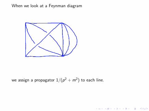
When we look at a Feynman diagram
we assign a propagator 1/(p2 + m2) to each line. We can write
1
p2 + m2=
∫ ∞0
dt exp(−t(p2 + m2)),
where t is the Schwinger parameter or proper time.
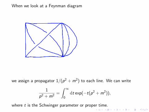
When we look at a Feynman diagram
we assign a propagator 1/(p2 + m2) to each line.
We can write
1
p2 + m2=
∫ ∞0
dt exp(−t(p2 + m2)),
where t is the Schwinger parameter or proper time.
When we look at a Feynman diagram
we assign a propagator 1/(p2 + m2) to each line. We can write
1
p2 + m2=
∫ ∞0
dt exp(−t(p2 + m2)),
where t is the Schwinger parameter or proper time.

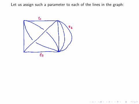
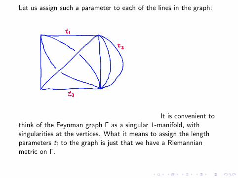
Let us assign such a parameter to each of the lines in the graph:
It is convenient tothink of the Feynman graph Γ as a singular 1-manifold, withsingularities at the vertices. What it means to assign the lengthparameters ti to the graph is just that we have a Riemannianmetric on Γ. Up to diffeomorphisms of the internal lines in Γ, theonly invariants of such a metric are the lengths of the linesegments, that is, the ti .
Let us assign such a parameter to each of the lines in the graph:
It is convenient tothink of the Feynman graph Γ as a singular 1-manifold, withsingularities at the vertices.
What it means to assign the lengthparameters ti to the graph is just that we have a Riemannianmetric on Γ. Up to diffeomorphisms of the internal lines in Γ, theonly invariants of such a metric are the lengths of the linesegments, that is, the ti .
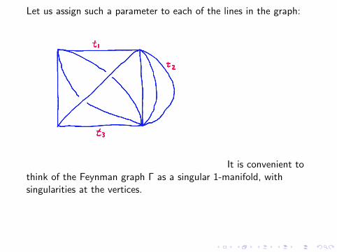
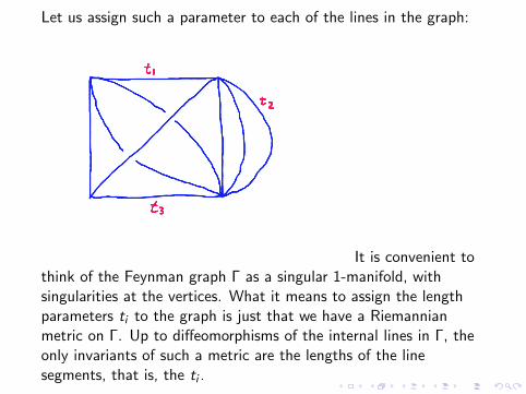
Let us assign such a parameter to each of the lines in the graph:
It is convenient tothink of the Feynman graph Γ as a singular 1-manifold, withsingularities at the vertices. What it means to assign the lengthparameters ti to the graph is just that we have a Riemannianmetric on Γ.
Up to diffeomorphisms of the internal lines in Γ, theonly invariants of such a metric are the lengths of the linesegments, that is, the ti .
Let us assign such a parameter to each of the lines in the graph:
It is convenient tothink of the Feynman graph Γ as a singular 1-manifold, withsingularities at the vertices. What it means to assign the lengthparameters ti to the graph is just that we have a Riemannianmetric on Γ. Up to diffeomorphisms of the internal lines in Γ, theonly invariants of such a metric are the lengths of the linesegments, that is, the ti .
Although each internal line in Γ has its own momentum pi , we donot just integrate over the pi independently: we have to imposemomentum conservation. Momentum conservation must beimposed at each vertex.
For a typical vertex
we want a delta function
(2π)4δ4(p1 + p2 + p3).
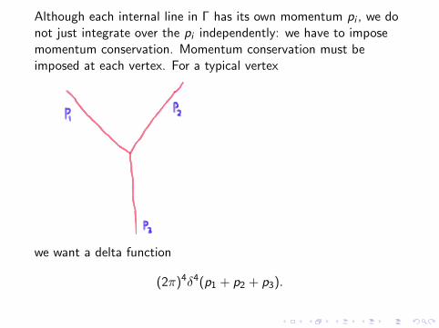
Although each internal line in Γ has its own momentum pi , we donot just integrate over the pi independently: we have to imposemomentum conservation. Momentum conservation must beimposed at each vertex. For a typical vertex
we want a delta function
(2π)4δ4(p1 + p2 + p3).
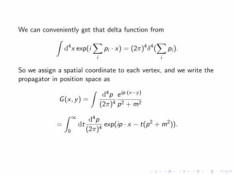
We can conveniently get that delta function from∫d4x exp(i
∑i
pi · x) = (2π)4δ4(∑i
pi ).
So we assign a spatial coordinate to each vertex, and we write thepropagator in position space as
G (x , y) =
∫d4p
(2π)4
e ip·(x−y)
p2 + m2
=
∫ ∞0
dtd4p
(2π)4exp(ip · x − t(p2 + m2)).

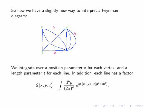
So now we have a slightly new way to interpret a Feynmandiagram:
We integrate over a position parameter x for each vertex, and alength parameter t for each line. In addition, each line has a factor
G (x , y ; t) =
∫d4p
(2π)4e ip·(x−y)−t(p2+m2).
So now we have a slightly new way to interpret a Feynmandiagram:
We integrate over a position parameter x for each vertex, and alength parameter t for each line. In addition, each line has a factor
G (x , y ; t) =
∫d4p
(2π)4e ip·(x−y)−t(p2+m2).
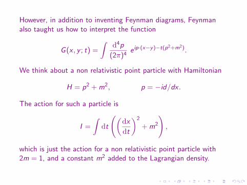
However, in addition to inventing Feynman diagrams, Feynmanalso taught us how to interpret the function
G (x , y ; t) =
∫d4p
(2π)4e ip·(x−y)−t(p2+m2).
We think about a non relativistic point particle with Hamiltonian
H = p2 + m2, p = −id/dx .
The action for such a particle is
I =
∫dt
((dx
dt
)2
+ m2
),
which is just the action for a non relativistic point particle with2m = 1, and a constant m2 added to the Lagrangian density.
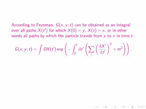
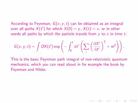
According to Feynman, G (x , y ; t) can be obtained as an integralover all paths X (t ′) for which X (0) = y , X (t) = x , or in otherwords all paths by which the particle travels from y to x in time t:
G (x , y ; t) =
∫DX (t ′) exp
(−∫ t
0dt ′
(∑i
(dX i
dt ′
)2
+ m2
)).
This is the basic Feynman path integral of non-relativistic quantummechanics, which you can read about in for example the book byFeynman and Hibbs.

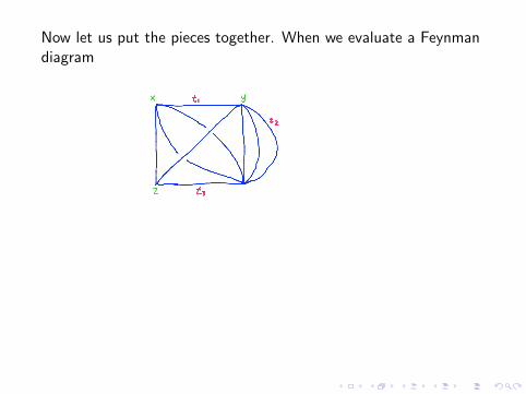
Now let us put the pieces together.
When we evaluate a Feynmandiagram
we integrate over all possible Riemannian metrics on the graph,which amounts to integrating over all length parameters t1, t2, . . . .We also integrate over all possible locations of the vertices x , y , zin space-time, and also over all possible maps of the linesconnecting the vertices into space-time. In other words, weintegrate over all possible maps of Γ into space-time.
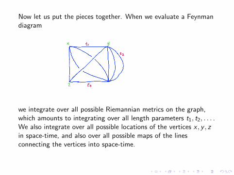
Now let us put the pieces together. When we evaluate a Feynmandiagram
we integrate over all possible Riemannian metrics on the graph,which amounts to integrating over all length parameters t1, t2, . . . .We also integrate over all possible locations of the vertices x , y , zin space-time, and also over all possible maps of the linesconnecting the vertices into space-time. In other words, weintegrate over all possible maps of Γ into space-time.
Now let us put the pieces together. When we evaluate a Feynmandiagram
we integrate over all possible Riemannian metrics on the graph,which amounts to integrating over all length parameters t1, t2, . . . .We also integrate over all possible locations of the vertices x , y , zin space-time, and also over all possible maps of the linesconnecting the vertices into space-time.
In other words, weintegrate over all possible maps of Γ into space-time.

Now let us put the pieces together. When we evaluate a Feynmandiagram
we integrate over all possible Riemannian metrics on the graph,which amounts to integrating over all length parameters t1, t2, . . . .We also integrate over all possible locations of the vertices x , y , zin space-time, and also over all possible maps of the linesconnecting the vertices into space-time. In other words, weintegrate over all possible maps of Γ into space-time.

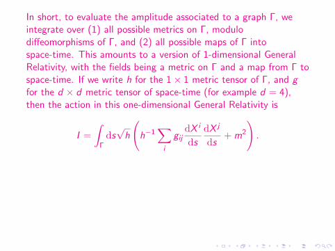
In short, to evaluate the amplitude associated to a graph Γ, weintegrate over (1) all possible metrics on Γ, modulodiffeomorphisms of Γ, and (2) all possible maps of Γ intospace-time.
This amounts to a version of 1-dimensional GeneralRelativity, with the fields being a metric on Γ and a map from Γ tospace-time. If we write h for the 1× 1 metric tensor of Γ, and gfor the d × d metric tensor of space-time (for example d = 4),then the action in this one-dimensional General Relativity is
I =
∫Γds√h
(h−1
∑i
gijdX i
ds
dX j
ds+ m2
).
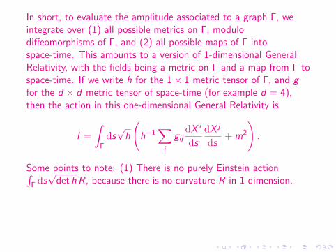
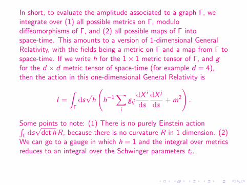
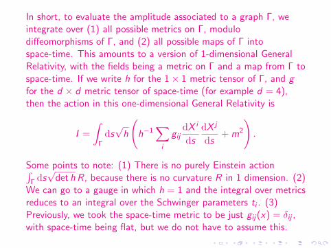
Some points to note: (1) There is no purely Einstein action∫Γ ds√
det h R, because there is no curvature R in 1 dimension. (2)We can go to a gauge in which h = 1 and the integral over metricsreduces to an integral over the Schwinger parameters ti . (3)Previously, we took the space-time metric to be just gij(x) = δij ,with space-time being flat, but we do not have to assume this.
In short, to evaluate the amplitude associated to a graph Γ, weintegrate over (1) all possible metrics on Γ, modulodiffeomorphisms of Γ, and (2) all possible maps of Γ intospace-time. This amounts to a version of 1-dimensional GeneralRelativity, with the fields being a metric on Γ and a map from Γ tospace-time.
If we write h for the 1× 1 metric tensor of Γ, and gfor the d × d metric tensor of space-time (for example d = 4),then the action in this one-dimensional General Relativity is
I =
∫Γds√h
(h−1
∑i
gijdX i
ds
dX j
ds+ m2
).
Some points to note: (1) There is no purely Einstein action∫Γ ds√
det h R, because there is no curvature R in 1 dimension. (2)We can go to a gauge in which h = 1 and the integral over metricsreduces to an integral over the Schwinger parameters ti . (3)Previously, we took the space-time metric to be just gij(x) = δij ,with space-time being flat, but we do not have to assume this.
In short, to evaluate the amplitude associated to a graph Γ, weintegrate over (1) all possible metrics on Γ, modulodiffeomorphisms of Γ, and (2) all possible maps of Γ intospace-time. This amounts to a version of 1-dimensional GeneralRelativity, with the fields being a metric on Γ and a map from Γ tospace-time. If we write h for the 1× 1 metric tensor of Γ, and gfor the d × d metric tensor of space-time (for example d = 4),then the action in this one-dimensional General Relativity is
I =
∫Γds√h
(h−1
∑i
gijdX i
ds
dX j
ds+ m2
).
Some points to note: (1) There is no purely Einstein action∫Γ ds√
det h R, because there is no curvature R in 1 dimension. (2)We can go to a gauge in which h = 1 and the integral over metricsreduces to an integral over the Schwinger parameters ti . (3)Previously, we took the space-time metric to be just gij(x) = δij ,with space-time being flat, but we do not have to assume this.

In short, to evaluate the amplitude associated to a graph Γ, weintegrate over (1) all possible metrics on Γ, modulodiffeomorphisms of Γ, and (2) all possible maps of Γ intospace-time. This amounts to a version of 1-dimensional GeneralRelativity, with the fields being a metric on Γ and a map from Γ tospace-time. If we write h for the 1× 1 metric tensor of Γ, and gfor the d × d metric tensor of space-time (for example d = 4),then the action in this one-dimensional General Relativity is
I =
∫Γds√h
(h−1
∑i
gijdX i
ds
dX j
ds+ m2
).
Some points to note:
(1) There is no purely Einstein action∫Γ ds√
det h R, because there is no curvature R in 1 dimension. (2)We can go to a gauge in which h = 1 and the integral over metricsreduces to an integral over the Schwinger parameters ti . (3)Previously, we took the space-time metric to be just gij(x) = δij ,with space-time being flat, but we do not have to assume this.
In short, to evaluate the amplitude associated to a graph Γ, weintegrate over (1) all possible metrics on Γ, modulodiffeomorphisms of Γ, and (2) all possible maps of Γ intospace-time. This amounts to a version of 1-dimensional GeneralRelativity, with the fields being a metric on Γ and a map from Γ tospace-time. If we write h for the 1× 1 metric tensor of Γ, and gfor the d × d metric tensor of space-time (for example d = 4),then the action in this one-dimensional General Relativity is
I =
∫Γds√h
(h−1
∑i
gijdX i
ds
dX j
ds+ m2
).
Some points to note: (1) There is no purely Einstein action∫Γ ds√
det h R, because there is no curvature R in 1 dimension.
(2)We can go to a gauge in which h = 1 and the integral over metricsreduces to an integral over the Schwinger parameters ti . (3)Previously, we took the space-time metric to be just gij(x) = δij ,with space-time being flat, but we do not have to assume this.
In short, to evaluate the amplitude associated to a graph Γ, weintegrate over (1) all possible metrics on Γ, modulodiffeomorphisms of Γ, and (2) all possible maps of Γ intospace-time. This amounts to a version of 1-dimensional GeneralRelativity, with the fields being a metric on Γ and a map from Γ tospace-time. If we write h for the 1× 1 metric tensor of Γ, and gfor the d × d metric tensor of space-time (for example d = 4),then the action in this one-dimensional General Relativity is
I =
∫Γds√h
(h−1
∑i
gijdX i
ds
dX j
ds+ m2
).
Some points to note: (1) There is no purely Einstein action∫Γ ds√
det h R, because there is no curvature R in 1 dimension. (2)We can go to a gauge in which h = 1 and the integral over metricsreduces to an integral over the Schwinger parameters ti .
(3)Previously, we took the space-time metric to be just gij(x) = δij ,with space-time being flat, but we do not have to assume this.
In short, to evaluate the amplitude associated to a graph Γ, weintegrate over (1) all possible metrics on Γ, modulodiffeomorphisms of Γ, and (2) all possible maps of Γ intospace-time. This amounts to a version of 1-dimensional GeneralRelativity, with the fields being a metric on Γ and a map from Γ tospace-time. If we write h for the 1× 1 metric tensor of Γ, and gfor the d × d metric tensor of space-time (for example d = 4),then the action in this one-dimensional General Relativity is
I =
∫Γds√h
(h−1
∑i
gijdX i
ds
dX j
ds+ m2
).
Some points to note: (1) There is no purely Einstein action∫Γ ds√
det h R, because there is no curvature R in 1 dimension. (2)We can go to a gauge in which h = 1 and the integral over metricsreduces to an integral over the Schwinger parameters ti . (3)Previously, we took the space-time metric to be just gij(x) = δij ,with space-time being flat, but we do not have to assume this.

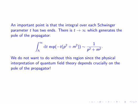
An important point is that the integral over each Schwingerparameter t has two ends. There is t →∞ which generates thepole of the propagator:∫ ∞
Λdt exp(−t(p2 + m2)) ∼ 1
p2 + m2.
We do not want to do without this region since the physicalinterpretation of quantum field theory depends crucially on thepole of the propagator!

The other end of the t integral is responsible for the fact that thepropagator is singular at short distances:∫ Λ
0dt
∫ddp
(2π)de ip·(x−y)−t(p2+m2) ∼ 1
|x − y |d−2.
This singular short distance behavior of the propagator comescompletely from the small t part of the integral.
This is where ultraviolet divergences come from.
When all theproper time parameters in a loop go to 0 and all the vertices in theloop map to (almost) the same point in space-time, we potentiallyrun into an ultraviolet divergence:
This is where ultraviolet divergences come from. When all theproper time parameters in a loop go to 0 and all the vertices in theloop map to (almost) the same point in space-time, we potentiallyrun into an ultraviolet divergence:

This is where ultraviolet divergences come from. When all theproper time parameters in a loop go to 0 and all the vertices in theloop map to (almost) the same point in space-time, we potentiallyrun into an ultraviolet divergence:

In quantum field theory, there is no way to get rid of the small tregion because if we put a lower cutoff on t, we would spoilspace-time locality.
This is the reason that quantum field theoriesare at risk of ultraviolet divergences.
In quantum field theory, there is no way to get rid of the small tregion because if we put a lower cutoff on t, we would spoilspace-time locality. This is the reason that quantum field theoriesare at risk of ultraviolet divergences.
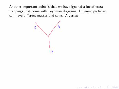
Another important point is that we have ignored a lot of extratrappings that come with Feynman diagrams. Different particlescan have different masses and spins.
A vertex
should be labeled by which types of particles are attached to it. Avertex has a coupling constant, which may depend on whichparticles are chosen. The Feynman rules may tell us to place at avertex not just a coupling “constant” but a more general factorthat may depend on the momenta or possibly the polarizations ofthe particles.
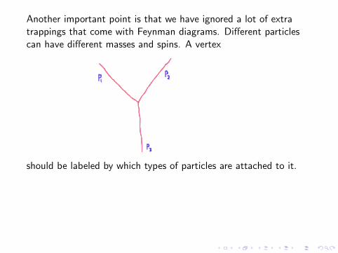
Another important point is that we have ignored a lot of extratrappings that come with Feynman diagrams. Different particlescan have different masses and spins. A vertex
should be labeled by which types of particles are attached to it. Avertex has a coupling constant, which may depend on whichparticles are chosen. The Feynman rules may tell us to place at avertex not just a coupling “constant” but a more general factorthat may depend on the momenta or possibly the polarizations ofthe particles.
Another important point is that we have ignored a lot of extratrappings that come with Feynman diagrams. Different particlescan have different masses and spins. A vertex
should be labeled by which types of particles are attached to it.
Avertex has a coupling constant, which may depend on whichparticles are chosen. The Feynman rules may tell us to place at avertex not just a coupling “constant” but a more general factorthat may depend on the momenta or possibly the polarizations ofthe particles.

Another important point is that we have ignored a lot of extratrappings that come with Feynman diagrams. Different particlescan have different masses and spins. A vertex
should be labeled by which types of particles are attached to it. Avertex has a coupling constant, which may depend on whichparticles are chosen.
The Feynman rules may tell us to place at avertex not just a coupling “constant” but a more general factorthat may depend on the momenta or possibly the polarizations ofthe particles.
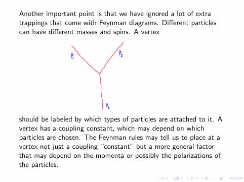
Another important point is that we have ignored a lot of extratrappings that come with Feynman diagrams. Different particlescan have different masses and spins. A vertex
should be labeled by which types of particles are attached to it. Avertex has a coupling constant, which may depend on whichparticles are chosen. The Feynman rules may tell us to place at avertex not just a coupling “constant” but a more general factorthat may depend on the momenta or possibly the polarizations ofthe particles.
These bells and whistles are what model-building in quantum fieldtheory is all about.
However, we have ignored them. We have justdescribed the properties that are common to all quantum fieldtheories.
These bells and whistles are what model-building in quantum fieldtheory is all about. However, we have ignored them.
We have justdescribed the properties that are common to all quantum fieldtheories.

These bells and whistles are what model-building in quantum fieldtheory is all about. However, we have ignored them. We have justdescribed the properties that are common to all quantum fieldtheories.
Now we move on to string theory, and I doubt it will surpriseanyone to be told that instead of doing 1-dimensional GeneralRelativity, we are now going to do 2-dimensional General Relativity.
Now in the starting point, we replace graphs by 2-dimensionalmanifolds, which are also called Riemann surfaces.
. I will callsuch a 2-manifold “the string worldsheet.”
Now we move on to string theory, and I doubt it will surpriseanyone to be told that instead of doing 1-dimensional GeneralRelativity, we are now going to do 2-dimensional General Relativity.Now in the starting point, we replace graphs by 2-dimensionalmanifolds, which are also called Riemann surfaces.
. I will callsuch a 2-manifold “the string worldsheet.”

Now we move on to string theory, and I doubt it will surpriseanyone to be told that instead of doing 1-dimensional GeneralRelativity, we are now going to do 2-dimensional General Relativity.Now in the starting point, we replace graphs by 2-dimensionalmanifolds, which are also called Riemann surfaces.
.
I will callsuch a 2-manifold “the string worldsheet.”

Now we move on to string theory, and I doubt it will surpriseanyone to be told that instead of doing 1-dimensional GeneralRelativity, we are now going to do 2-dimensional General Relativity.Now in the starting point, we replace graphs by 2-dimensionalmanifolds, which are also called Riemann surfaces.
. I will callsuch a 2-manifold “the string worldsheet.”
One thing we note immediately is that there is no need to assumesingularities and hence a lot of the bells and whistles of quantumfield theory will not have analogs.
Unlike a Feynman graph, whichis divided into different lines, which can represent particles ofdifferent types with different masses and spins, any part of a stringworldsheet is equivalent to any other so “there is only one string.”Whatever particles there are going to be represent different statesof vibration of one basic string. Also there are not any vertices inthe string worldsheet so we do not have the freedom to tell thestring how to interact.
One thing we note immediately is that there is no need to assumesingularities and hence a lot of the bells and whistles of quantumfield theory will not have analogs. Unlike a Feynman graph, whichis divided into different lines, which can represent particles ofdifferent types with different masses and spins, any part of a stringworldsheet is equivalent to any other so “there is only one string.”
Whatever particles there are going to be represent different statesof vibration of one basic string. Also there are not any vertices inthe string worldsheet so we do not have the freedom to tell thestring how to interact.

One thing we note immediately is that there is no need to assumesingularities and hence a lot of the bells and whistles of quantumfield theory will not have analogs. Unlike a Feynman graph, whichis divided into different lines, which can represent particles ofdifferent types with different masses and spins, any part of a stringworldsheet is equivalent to any other so “there is only one string.”Whatever particles there are going to be represent different statesof vibration of one basic string.
Also there are not any vertices inthe string worldsheet so we do not have the freedom to tell thestring how to interact.
One thing we note immediately is that there is no need to assumesingularities and hence a lot of the bells and whistles of quantumfield theory will not have analogs. Unlike a Feynman graph, whichis divided into different lines, which can represent particles ofdifferent types with different masses and spins, any part of a stringworldsheet is equivalent to any other so “there is only one string.”Whatever particles there are going to be represent different statesof vibration of one basic string. Also there are not any vertices inthe string worldsheet so we do not have the freedom to tell thestring how to interact.

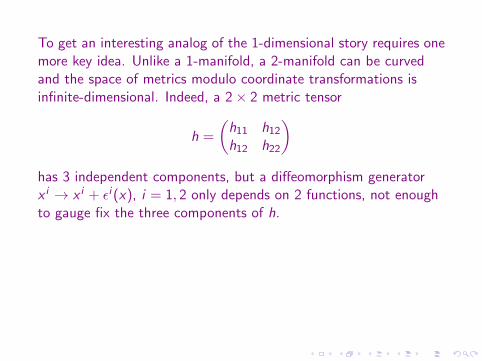
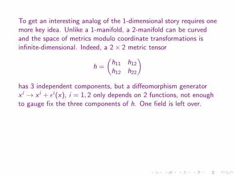
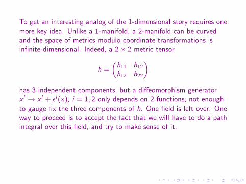
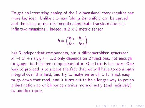
To get an interesting analog of the 1-dimensional story requires onemore key idea.
Unlike a 1-manifold, a 2-manifold can be curvedand the space of metrics modulo coordinate transformations isinfinite-dimensional. Indeed, a 2× 2 metric tensor
h =
(h11 h12
h12 h22
)has 3 independent components, but a diffeomorphism generatorx i → x i + εi (x), i = 1, 2 only depends on 2 functions, not enoughto gauge fix the three components of h. One field is left over. Oneway to proceed is to accept the fact that we will have to do a pathintegral over this field, and try to make sense of it. It is not easyto go down that road, and it turns out to be a longer way to get toa destination at which we can arrive more directly (and incisively)by another route.
To get an interesting analog of the 1-dimensional story requires onemore key idea. Unlike a 1-manifold, a 2-manifold can be curvedand the space of metrics modulo coordinate transformations isinfinite-dimensional.
Indeed, a 2× 2 metric tensor
h =
(h11 h12
h12 h22
)has 3 independent components, but a diffeomorphism generatorx i → x i + εi (x), i = 1, 2 only depends on 2 functions, not enoughto gauge fix the three components of h. One field is left over. Oneway to proceed is to accept the fact that we will have to do a pathintegral over this field, and try to make sense of it. It is not easyto go down that road, and it turns out to be a longer way to get toa destination at which we can arrive more directly (and incisively)by another route.
To get an interesting analog of the 1-dimensional story requires onemore key idea. Unlike a 1-manifold, a 2-manifold can be curvedand the space of metrics modulo coordinate transformations isinfinite-dimensional. Indeed, a 2× 2 metric tensor
h =
(h11 h12
h12 h22
)has 3 independent components, but a diffeomorphism generatorx i → x i + εi (x), i = 1, 2 only depends on 2 functions, not enoughto gauge fix the three components of h.
One field is left over. Oneway to proceed is to accept the fact that we will have to do a pathintegral over this field, and try to make sense of it. It is not easyto go down that road, and it turns out to be a longer way to get toa destination at which we can arrive more directly (and incisively)by another route.
To get an interesting analog of the 1-dimensional story requires onemore key idea. Unlike a 1-manifold, a 2-manifold can be curvedand the space of metrics modulo coordinate transformations isinfinite-dimensional. Indeed, a 2× 2 metric tensor
h =
(h11 h12
h12 h22
)has 3 independent components, but a diffeomorphism generatorx i → x i + εi (x), i = 1, 2 only depends on 2 functions, not enoughto gauge fix the three components of h. One field is left over.
Oneway to proceed is to accept the fact that we will have to do a pathintegral over this field, and try to make sense of it. It is not easyto go down that road, and it turns out to be a longer way to get toa destination at which we can arrive more directly (and incisively)by another route.
To get an interesting analog of the 1-dimensional story requires onemore key idea. Unlike a 1-manifold, a 2-manifold can be curvedand the space of metrics modulo coordinate transformations isinfinite-dimensional. Indeed, a 2× 2 metric tensor
h =
(h11 h12
h12 h22
)has 3 independent components, but a diffeomorphism generatorx i → x i + εi (x), i = 1, 2 only depends on 2 functions, not enoughto gauge fix the three components of h. One field is left over. Oneway to proceed is to accept the fact that we will have to do a pathintegral over this field, and try to make sense of it.
It is not easyto go down that road, and it turns out to be a longer way to get toa destination at which we can arrive more directly (and incisively)by another route.
To get an interesting analog of the 1-dimensional story requires onemore key idea. Unlike a 1-manifold, a 2-manifold can be curvedand the space of metrics modulo coordinate transformations isinfinite-dimensional. Indeed, a 2× 2 metric tensor
h =
(h11 h12
h12 h22
)has 3 independent components, but a diffeomorphism generatorx i → x i + εi (x), i = 1, 2 only depends on 2 functions, not enoughto gauge fix the three components of h. One field is left over. Oneway to proceed is to accept the fact that we will have to do a pathintegral over this field, and try to make sense of it. It is not easyto go down that road, and it turns out to be a longer way to get toa destination at which we can arrive more directly (and incisively)by another route.
The other route is as follows.
We get something nice if we imposean extra symmetry that eliminates 1 component of h. We do thatby requiring conformal or Weyl invariance
hij ∼= hije2σ
for any function σ.

The other route is as follows. We get something nice if we imposean extra symmetry that eliminates 1 component of h.
We do thatby requiring conformal or Weyl invariance
hij ∼= hije2σ
for any function σ.
The other route is as follows. We get something nice if we imposean extra symmetry that eliminates 1 component of h. We do thatby requiring conformal or Weyl invariance
hij ∼= hije2σ
for any function σ.
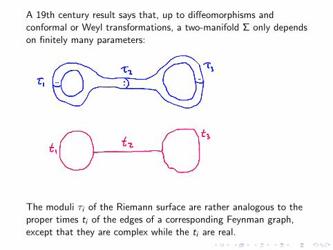
A 19th century result says that, up to diffeomorphisms andconformal or Weyl transformations, a two-manifold Σ only dependson finitely many parameters:
The moduli τi of the Riemann surface are rather analogous to theproper times ti of the edges of a corresponding Feynman graph,except that they are complex while the ti are real.
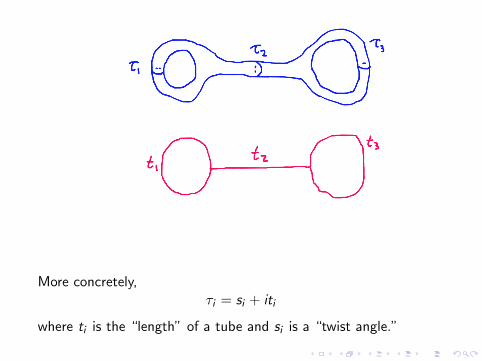
More concretely,τi = si + iti
where ti is the “length” of a tube and si is a “twist angle.”
Just as in 1 dimension, we are going to add “matter” to our2-dimensional gravity theory.
Since we are trying to use conformalinvariance to improve the analogy between 2 dimensions and 1dimension, by reducing the integral over 2-dimensional metrics toan integral over finitely many parameters τi , the “matter” part ofthe action has to be conformally invariant. For instance, in 2dimensions, the usual action for massless scalar fields isconformally invariant:
I =
∫Σd2σ
√det g
(gαβ∂αX
I∂βXJGIJ(X )
).
The X ’s describe a map from the two-manifold Σ to a spacetimeM, which can have D dimensions and which I’ve endowed with ametric tensor GIJ(X ).

Just as in 1 dimension, we are going to add “matter” to our2-dimensional gravity theory. Since we are trying to use conformalinvariance to improve the analogy between 2 dimensions and 1dimension, by reducing the integral over 2-dimensional metrics toan integral over finitely many parameters τi , the “matter” part ofthe action has to be conformally invariant.
For instance, in 2dimensions, the usual action for massless scalar fields isconformally invariant:
I =
∫Σd2σ
√det g
(gαβ∂αX
I∂βXJGIJ(X )
).
The X ’s describe a map from the two-manifold Σ to a spacetimeM, which can have D dimensions and which I’ve endowed with ametric tensor GIJ(X ).

Just as in 1 dimension, we are going to add “matter” to our2-dimensional gravity theory. Since we are trying to use conformalinvariance to improve the analogy between 2 dimensions and 1dimension, by reducing the integral over 2-dimensional metrics toan integral over finitely many parameters τi , the “matter” part ofthe action has to be conformally invariant. For instance, in 2dimensions, the usual action for massless scalar fields isconformally invariant:
I =
∫Σd2σ
√det g
(gαβ∂αX
I∂βXJGIJ(X )
).
The X ’s describe a map from the two-manifold Σ to a spacetimeM, which can have D dimensions and which I’ve endowed with ametric tensor GIJ(X ).

There is still (almost) no purely gravitational action in twodimensions since the Einstein-Hilbert action∫
Σd2σ√
det h R
is a total derivative (topological invariant).
So just as in ordinaryquantum field theory, we basically have to only consider the actionfor the matter fields.
There is still (almost) no purely gravitational action in twodimensions since the Einstein-Hilbert action∫
Σd2σ√
det h R
is a total derivative (topological invariant). So just as in ordinaryquantum field theory, we basically have to only consider the actionfor the matter fields.
To develop the theory, we are supposed to (i) for a fixed Σ, do aFeynman path integral over the fields X = (X 1, . . . ,XD), and (ii)then integrate over the moduli τ1, τ2, . . . and sum over alltopological choices for Σ. The last step is the analog of summingover all Feynman graphs in ordinary field theory.
To understand why the ultraviolet divergences go away, let usconsider the basic 1-loop contribution to the vacuum energy.
Asimple example of a divergent 1-loop contribution to the vacuumenergy comes from a scalar field of mass m. Its path integral gives
1√det(−∇2 + m2)
= exp(−1
2Tr log(−∇2 + m2)).
This means that the 1-loop contribution to the effective action is
I ∗ =1
2Tr log(−∇2 + m2) =
1
2
∫ ∞0
dt
texp(−tH)
where H = p2 + m2 = −∇2 + m2.
To understand why the ultraviolet divergences go away, let usconsider the basic 1-loop contribution to the vacuum energy. Asimple example of a divergent 1-loop contribution to the vacuumenergy comes from a scalar field of mass m.
Its path integral gives
1√det(−∇2 + m2)
= exp(−1
2Tr log(−∇2 + m2)).
This means that the 1-loop contribution to the effective action is
I ∗ =1
2Tr log(−∇2 + m2) =
1
2
∫ ∞0
dt
texp(−tH)
where H = p2 + m2 = −∇2 + m2.

To understand why the ultraviolet divergences go away, let usconsider the basic 1-loop contribution to the vacuum energy. Asimple example of a divergent 1-loop contribution to the vacuumenergy comes from a scalar field of mass m. Its path integral gives
1√det(−∇2 + m2)
= exp(−1
2Tr log(−∇2 + m2)).
This means that the 1-loop contribution to the effective action is
I ∗ =1
2Tr log(−∇2 + m2) =
1
2
∫ ∞0
dt
texp(−tH)
where H = p2 + m2 = −∇2 + m2.
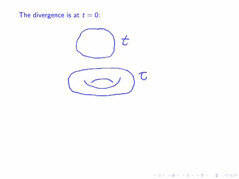
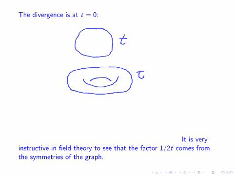
The divergence is at t = 0:
It is veryinstructive in field theory to see that the factor 1/2t comes fromthe symmetries of the graph.
The divergence is at t = 0:
It is veryinstructive in field theory to see that the factor 1/2t comes fromthe symmetries of the graph.
This integral diverges for t → 0. What we are about to see is thatthe string theory problem is similar, except that the integral onlygoes over t ≥ 1, so there will be no divergence.
(I will take a shortcut and assume the torus is conformallyequivalent to a rectangle with opposite sides glued together ratherthan a more general parallelogram. This doesn’t affect theconclusion, but it shortens the explanation.)
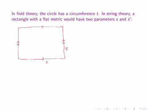
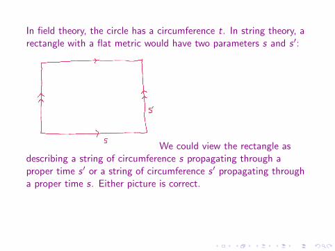
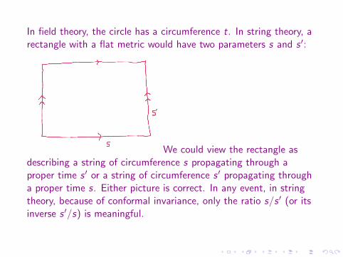
In field theory, the circle has a circumference t. In string theory, arectangle with a flat metric would have two parameters s and s ′:
We could view the rectangle asdescribing a string of circumference s propagating through aproper time s ′ or a string of circumference s ′ propagating througha proper time s. Either picture is correct. In any event, in stringtheory, because of conformal invariance, only the ratio s/s ′ (or itsinverse s ′/s) is meaningful.
In field theory, the circle has a circumference t. In string theory, arectangle with a flat metric would have two parameters s and s ′:
We could view the rectangle asdescribing a string of circumference s propagating through aproper time s ′ or a string of circumference s ′ propagating througha proper time s. Either picture is correct.
In any event, in stringtheory, because of conformal invariance, only the ratio s/s ′ (or itsinverse s ′/s) is meaningful.
In field theory, the circle has a circumference t. In string theory, arectangle with a flat metric would have two parameters s and s ′:
We could view the rectangle asdescribing a string of circumference s propagating through aproper time s ′ or a string of circumference s ′ propagating througha proper time s. Either picture is correct. In any event, in stringtheory, because of conformal invariance, only the ratio s/s ′ (or itsinverse s ′/s) is meaningful.
The string theory formula will reduce approximately to field theoryif, say, s >> s ′. Then we can think in terms of a string ofcircumference s ′ propagating for a proper time s. Because ofconformal invariance we can set s ′ = 1 and identify s with theproper time t of a field theory: t = s/s ′ = s. So the integral thatin field theory is an integral over the proper time t is in stringtheory replaced by an integral over the ratio s/s ′.
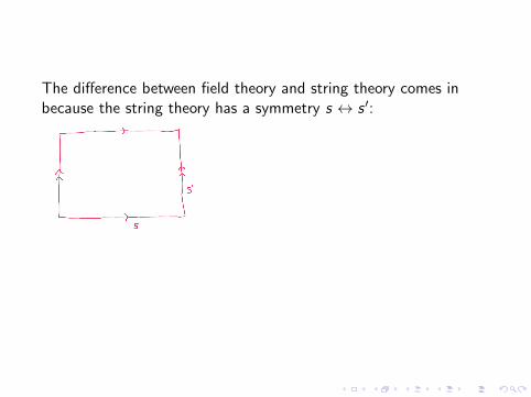
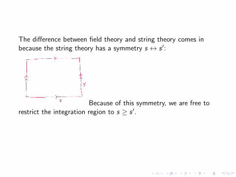
The difference between field theory and string theory comes inbecause the string theory has a symmetry s ↔ s ′:
Because of this symmetry, we are free torestrict the integration region to s ≥ s ′. In other words, if we sett = s/s ′, we are restricted to t ≥ 1.
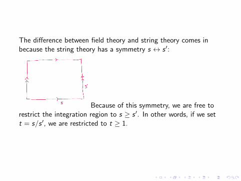
The difference between field theory and string theory comes inbecause the string theory has a symmetry s ↔ s ′:
Because of this symmetry, we are free torestrict the integration region to s ≥ s ′. In other words, if we sett = s/s ′, we are restricted to t ≥ 1.
The difference between field theory and string theory comes inbecause the string theory has a symmetry s ↔ s ′:
Because of this symmetry, we are free torestrict the integration region to s ≥ s ′.
In other words, if we sett = s/s ′, we are restricted to t ≥ 1.
The difference between field theory and string theory comes inbecause the string theory has a symmetry s ↔ s ′:
Because of this symmetry, we are free torestrict the integration region to s ≥ s ′. In other words, if we sett = s/s ′, we are restricted to t ≥ 1.
In short, in field theory we integrate over t from 0 to ∞ and wetypically find ultraviolet divergences for t → 0.
(Depending on thetheory, we may find infrared divergences for t →∞.) In stringtheory, we integrate over t from 1 to ∞. There is no ultravioletdivergence since the integral begins at 1. (Depending on thetheory, there may be an infrared divergence for t →∞.)
In short, in field theory we integrate over t from 0 to ∞ and wetypically find ultraviolet divergences for t → 0. (Depending on thetheory, we may find infrared divergences for t →∞.)
In stringtheory, we integrate over t from 1 to ∞. There is no ultravioletdivergence since the integral begins at 1. (Depending on thetheory, there may be an infrared divergence for t →∞.)
In short, in field theory we integrate over t from 0 to ∞ and wetypically find ultraviolet divergences for t → 0. (Depending on thetheory, we may find infrared divergences for t →∞.) In stringtheory, we integrate over t from 1 to ∞. There is no ultravioletdivergence since the integral begins at 1.
(Depending on thetheory, there may be an infrared divergence for t →∞.)
In short, in field theory we integrate over t from 0 to ∞ and wetypically find ultraviolet divergences for t → 0. (Depending on thetheory, we may find infrared divergences for t →∞.) In stringtheory, we integrate over t from 1 to ∞. There is no ultravioletdivergence since the integral begins at 1. (Depending on thetheory, there may be an infrared divergence for t →∞.)

I have explained this in a slightly naive way, but the point holdstrue in general.
Technically, the moduli space of Riemann surfaceshas a region “at infinity” that corresponds to the infrared regiont →∞ in field theory. But it has no region corresponding to theultraviolet region t → 0 in field theory. So string theory is free ofthe ultraviolet divergences of field theory.
What is true but much less trivial is the following statement: Theinfrared behavior of string theory matches the infrared behavior ofa field theory with appropriate light particles and interactions.
I have explained this in a slightly naive way, but the point holdstrue in general.Technically, the moduli space of Riemann surfaceshas a region “at infinity” that corresponds to the infrared regiont →∞ in field theory.
But it has no region corresponding to theultraviolet region t → 0 in field theory. So string theory is free ofthe ultraviolet divergences of field theory.
What is true but much less trivial is the following statement: Theinfrared behavior of string theory matches the infrared behavior ofa field theory with appropriate light particles and interactions.
I have explained this in a slightly naive way, but the point holdstrue in general.Technically, the moduli space of Riemann surfaceshas a region “at infinity” that corresponds to the infrared regiont →∞ in field theory. But it has no region corresponding to theultraviolet region t → 0 in field theory.
So string theory is free ofthe ultraviolet divergences of field theory.
What is true but much less trivial is the following statement: Theinfrared behavior of string theory matches the infrared behavior ofa field theory with appropriate light particles and interactions.

I have explained this in a slightly naive way, but the point holdstrue in general.Technically, the moduli space of Riemann surfaceshas a region “at infinity” that corresponds to the infrared regiont →∞ in field theory. But it has no region corresponding to theultraviolet region t → 0 in field theory. So string theory is free ofthe ultraviolet divergences of field theory.
What is true but much less trivial is the following statement: Theinfrared behavior of string theory matches the infrared behavior ofa field theory with appropriate light particles and interactions.

By now I have done what I said at the beginning,
but theorganizers are so generous with the time that I will explain onemore thing: why string theory describes gravity in the targetspacetime, which I call M. This isn’t up to us; it happensautomatically. To explain this takes a couple of steps.
By now I have done what I said at the beginning, but theorganizers are so generous with the time that I will explain onemore thing: why string theory describes gravity in the targetspacetime, which I call M.
This isn’t up to us; it happensautomatically. To explain this takes a couple of steps.

By now I have done what I said at the beginning, but theorganizers are so generous with the time that I will explain onemore thing: why string theory describes gravity in the targetspacetime, which I call M. This isn’t up to us; it happensautomatically.
To explain this takes a couple of steps.

By now I have done what I said at the beginning, but theorganizers are so generous with the time that I will explain onemore thing: why string theory describes gravity in the targetspacetime, which I call M. This isn’t up to us; it happensautomatically. To explain this takes a couple of steps.

First of all, what are the fields in the target space theory?
In thefamiliar case, they are the external lines in a Feynman diagram. Soin the present case, the fields in the target space are the externalstrings:
In other words, the fields are the vibrational states of a string.
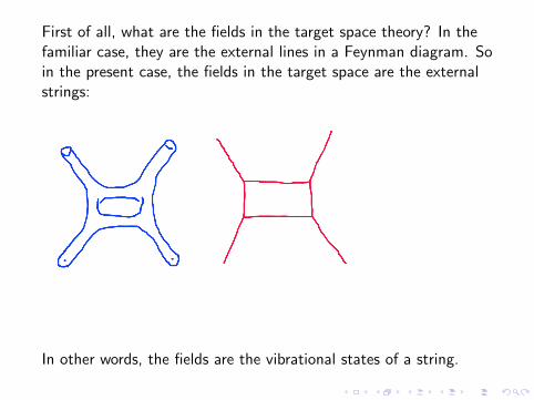
First of all, what are the fields in the target space theory? In thefamiliar case, they are the external lines in a Feynman diagram.
Soin the present case, the fields in the target space are the externalstrings:
In other words, the fields are the vibrational states of a string.

First of all, what are the fields in the target space theory? In thefamiliar case, they are the external lines in a Feynman diagram. Soin the present case, the fields in the target space are the externalstrings:
In other words, the fields are the vibrational states of a string.
First of all, what are the fields in the target space theory? In thefamiliar case, they are the external lines in a Feynman diagram. Soin the present case, the fields in the target space are the externalstrings:
In other words, the fields are the vibrational states of a string.
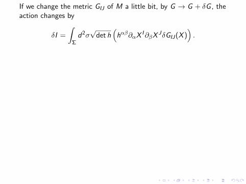
If we change the metric GIJ of M a little bit, by G → G + δG , theaction changes by
δI =
∫Σd2σ√
det h(hαβ∂αX
I∂βXJδGIJ(X )
).
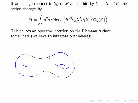
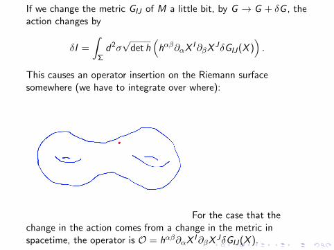
This causes an operator insertion on the Riemann surfacesomewhere (we have to integrate over where):
For the case that thechange in the action comes from a change in the metric inspacetime, the operator is O = hαβ∂αX
I∂βXJδGIJ(X ).
If we change the metric GIJ of M a little bit, by G → G + δG , theaction changes by
δI =
∫Σd2σ√
det h(hαβ∂αX
I∂βXJδGIJ(X )
).
This causes an operator insertion on the Riemann surfacesomewhere (we have to integrate over where):
For the case that thechange in the action comes from a change in the metric inspacetime, the operator is O = hαβ∂αX
I∂βXJδGIJ(X ).
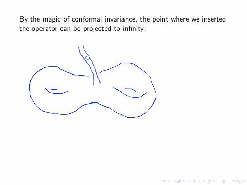
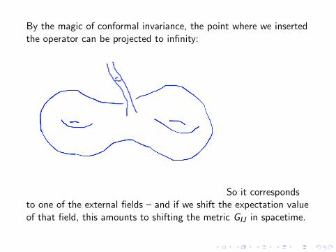
By the magic of conformal invariance, the point where we insertedthe operator can be projected to infinity:
So it correspondsto one of the external fields – and if we shift the expectation valueof that field, this amounts to shifting the metric GIJ in spacetime.
By the magic of conformal invariance, the point where we insertedthe operator can be projected to infinity:
So it correspondsto one of the external fields – and if we shift the expectation valueof that field, this amounts to shifting the metric GIJ in spacetime.
So the dynamics of gravity in spacetime is part of what stringtheory describes.
A shift in the metric of spacetime is a shift in theexpectation value of one of the string fields; or differently put, oneof the string fields is the spacetime metric.
So the dynamics of gravity in spacetime is part of what stringtheory describes. A shift in the metric of spacetime is a shift in theexpectation value of one of the string fields; or differently put, oneof the string fields is the spacetime metric.

Going down this road (and incorporating spacetime supersymmetryto avoid some infrared problems), one arrives at a systematic wayto calculate quantum processes involving gravitons, free of theultraviolet divergences that one gets if one tries to quantizeEinstein’s theory directly.
The ultraviolet divergences are absentbecause two-dimensional conformal invariance completelyeliminates the ultraviolet region from the Feynman diagrams.
Going down this road (and incorporating spacetime supersymmetryto avoid some infrared problems), one arrives at a systematic wayto calculate quantum processes involving gravitons, free of theultraviolet divergences that one gets if one tries to quantizeEinstein’s theory directly. The ultraviolet divergences are absentbecause two-dimensional conformal invariance completelyeliminates the ultraviolet region from the Feynman diagrams.