Efficient Manifold Ranking for Image Retrieval

Bin Xu1, Jiajun Bu1, Chun Chen1, Deng Cai2, Xiaofei He2, Wei Liu3, Jiebo Luo4

1Zhejiang Provincial Key Laboratory of Service RobotCollege of Computer Science, Zhejiang University, Hangzhou, China

{xbzju,bjj,chenc,hezhanying}@zju.edu.cn2State Key Lab of CAD&CG, College of Computer Science, Zhejiang University, Hangzhou, China

{dengcai,xiaofeihe}@cad.zju.edu.cn3Columbia University, New York, NY, USA, wliu@ee.columbia.edu

4Kodak Research Laboratories, Eastman Kodak Company, Rochester, NY, USA, jiebo.luo@kodak.com

ABSTRACTManifold Ranking (MR), a graph-based ranking algorithm,has been widely applied in information retrieval and shownto have excellent performance and feasibility on a varietyof data types. Particularly, it has been successfully appliedto content-based image retrieval, because of its outstandingability to discover underlying geometrical structure of thegiven image database. However, manifold ranking is com-putationally very expensive, both in graph construction andranking computation stages, which significantly limits its ap-plicability to very large data sets. In this paper, we extendthe original manifold ranking algorithm and propose a newframework named Efficient Manifold Ranking (EMR). Weaim to address the shortcomings of MR from two perspec-tives: scalable graph construction and efficient computation.Specifically, we build an anchor graph on the data set insteadof the traditional k-nearest neighbor graph, and design a newform of adjacency matrix utilized to speed up the rankingcomputation. The experimental results on a real world im-age database demonstrate the effectiveness and efficiency ofour proposed method. With a comparable performance tothe original manifold ranking, our method significantly re-duces the computational time, makes it a promising methodto large scale real world retrieval problems.

Categories and Subject DescriptorsH.3.3 [Information Search and Retrieval]: Retrievalmodels; H.2.8 [Database Applications]: Image databases

General TermsAlgorithm, Performance

KeywordsEfficient manifold ranking, image retrieval, graph-based al-gorithm, out-of-sample

Permission to make digital or hard copies of all or part of this work forpersonal or classroom use is granted without fee provided that copies arenot made or distributed for profit or commercial advantage and that copiesbear this notice and the full citation on the first page. To copy otherwise, torepublish, to post on servers or to redistribute to lists, requires prior specificpermission and/or a fee.SIGIR’11 July 24–28, 2011, Beijing, ChinaCopyright 2011 ACM 978-1-4503-0757-4/11/07 ...$10.00.

1. INTRODUCTIONTraditional image retrieval systems are based on keyword

search, such as Google and Yahoo image search. In thesesystems, user keyword is matched with the context aroundan image including the title, manual annotation, web doc-ument, etc. These systems don’t utilize information fromimages. However these systems suffer many problems, suchas shortage of the text information and inconsistency of themeaning of the text and image.

Content-based image retrieval (CBIR) is a considerablechoice to overcome these difficulties. CBIR has drawed agreat attention in the past two decades [5, 19, 27]. Differ-ent from traditional keyword search systems, CBIR systemsutilize the low-level features (color, texture, shape, etc.),automatically extracted from images. This is a vital char-acter for efficient management and search in a large imagedatabase. But the low-level features used in CBIR systemsare often visually characterized, and with no direct connec-tion with semantic concepts of the images. How to narrowthe semantic gap has been the main challenge for CBIR.

Many data sets have underlying cluster or manifold struc-ture. Under such circumstances, the assumption of label con-sistency is reasonable [23, 36]. It means that those nearbydata points, or points belong to the same cluster or mani-fold, are very likely to share the same semantic label. Thisphenomenon is extremely important to explore the seman-tic relevance when the label information is unknown. Thus,a good CBIR method should consider low-level features aswell as intrinsic structure of the data.

Manifold Ranking (MR) [36,37], a semi-supervised graph-based ranking algorithm, has been widely applied in infor-mation retrieval, and shown to have excellent performanceand feasibility on a variety of data types, such as the text[28], image [9], and video [34]. The core idea of manifoldranking is to rank the data with respect to the intrinsicstructure collectively revealed by a large number of data.By taking the underlying structure into account, manifoldranking assigns each data point a relative ranking score, in-stead of an absolute pairwise similarity as traditional ways.The score is treated as a distance metric defined on the man-ifold, which is more meaningful to capturing the semanticrelevance degree. He et al. [9] firstly applied manifold rank-ing to CBIR, and significantly improved image retrieval per-formance compared with state-of-the-art algorithms.

However, manifold ranking has its own drawbacks to han-dle large scale data sets – it has expensive computational

525

cost, both in graph construction and ranking computationstages. Particularly, it is costly to handle an out-of-samplequery (a new sample). That means original manifold rank-ing is inadequate for a real world CBIR system, in whichthe user provided query is always an out-of-sample. It’s in-tolerable for a user to wait a long time to get returns.

In this paper, we extend the original manifold ranking andpropose a novel framework named Efficient Manifold Rank-ing (EMR). We try to address the shortcomings of manifoldranking from two perspectives: the first is scalable graphconstruction; and the second is efficient computation, espe-cially for out-of-sample retrieval. The main contributions ofthis paper are as follows. (1) Based on the anchor graphconstruction [18,35], we design a new form of adjacency ma-trix and give it an intuitive explanation. (2) By the newform, our method EMR achieves a comparable performanceto original manifold ranking but significantly reduces thecomputational time.

The rest of this paper is organized as follows. In section2, we briefly discuss some related works and in section 3, wereview the manifold ranking algorithm and make a detailedanalysis. The proposed approach EMR is described in sec-tion 4. In section 5, we present the experiment results on areal world image database. Finally we provide an extensionanalysis in section 6 and conclusions in section 7.

2. RELATED WORKIn this section, we discuss two most relevant topics to our

work: ranking model and content-based image retrieval.The problem of ranking has recently gained great atten-

tions in both information retrieval and machine learningareas. Conventional ranking models can be content basedmodels, like the Vector Space Model, BM25, and the lan-guage modeling [22]; or link structure based models, like thefamous PageRank [2] and HITS [15]; or cross media mod-els [13]. Another important category is the learning to rankmodel, which aims to optimize a ranking function that incor-porates relevance features and avoids tuning a large numberof parameters empirically [7, 26]. However, many conven-tional models ignore the important issue of efficiency, whichis crucial for a real-time systems, such as a web application.In [29], the authors present a unified framework for jointlyoptimizing effectiveness and efficiency.

2.1 Graph-based RankingIn this paper, we focus on a particular kind of ranking

model – graph-based ranking. It has been successfully ap-plied in link-structure analysis of the web [2, 15] and socialnetworks research [3, 8, 17]. Generally, a graph can be de-noted as G = (V,E,W ), where V is a set of vertices in whicheach vertex represents a data point, E ⊆ V × V is a set ofedges connecting related vertices, and W is a adjacency ma-trix recording the pairwise weights between vertices. Theobject of a graph-based ranking model is to decide the im-portance of a vertex in a graph, based on local or globalinformation draw from the graph.

Agarwal [1] proposed to model the data by a weightedgraph, and incorporated this graph structure into the rank-ing function as a regularizer. Guan et al. [8] proposed agraph-based ranking algorithm for interrelated multi-typeresources to generate personalized tag recommendation. Liuet al. [17] proposed an automatically tag ranking scheme byperforming a random walk over a tag similarity graph. In [3],

the authors made the music recommendation by ranking ona unified hypergraph, combining with rich social informationand music content. Recently, there have been some paperson speeding up manifold ranking. In [11], the authors parti-tioned the data into several parts and computed the rankingfunction by a block-wise way.

2.2 Content-based Image RetrievalIn many cases, we have no more information than the data

itself. Without label information, capturing semantic rela-tionship between images is quite difficult. A great amount ofresearches have been performed for designing more informa-tive low-level features (e.g., SIFT features [20]) to representimages, or better metrics (e.g., DPF [16]) to measure theperceptual similarity, but their performance is restricted bymany conditions and is sensitive to the data. Relevancefeedback [24] is a powerful tool for interactive CBIR. User’shigh level perception is captured by dynamically updatedweights based on the user’s feedback.

Many traditional image retrieval methods focus on thedata features too much, and they ignore the underlyingstructure information, which is of great importance for se-mantic discovery, especially when the label information isunknown. A good CBIR method should consider the imagefeatures as well as the intrinsic structure of the data, in ouropinion. Manifold ranking [36,37] ranks data with respect tothe intrinsic geometrical structure, which is exactly in linewith our consideration.

3. MANIFOLD RANKING REVIEWIn this section, we briefly review the manifold ranking

algorithm and make a detailed analysis about its drawbacks.We start form the description of notations.

3.1 Notations and FormulationsGiven a set of data χ = {x1, x2, . . . , xn} ⊂ Rm and build

a graph on the data (e.g., kNN graph). W ∈ Rn×n denotesthe adjacency matrix with element wij saving the weight ofthe edge between point i and j. Normally the weight canbe defined by the heat kernel wij = exp[−d2(xi, xj)/2σ

2)] ifthere is an edge linking xi and xj , otherwise wij = 0. Func-tion d(xi, xj) is a distance metric of xi and xj defined on χ,such as the Euclidean distance. Let r : χ → R be a rank-ing function which assigns to each point xi a ranking scoreri. Finally, we define an initial vector y = [y1, . . . , yn]

T , inwhich yi = 1 if xi is a query and yi = 0 otherwise.

The cost function associated with r is defined to be

O(r) =1

2(

n∑i,j=1

wij‖ 1√Dii

ri − 1√Djj

rj‖2 +μ

n∑i=1

‖ri − yi‖2),

(1)where μ > 0 is the regularization parameter and D is adiagonal matrix with Dii =

∑nj=1 wij .

The first term in the cost function is a smoothness con-straint, which makes the nearby points in the space haveclose ranking scores. The second term is a fitting constraint,which means the ranking result should fit to the initial labelassignment. If we have more prior knowledge about the rel-evance or confidence of each query, we can assign differentinitial scores to the queries. Minimizing the cost function

526

O(r), we get the optimal r by the following closed form

r∗ = (In − αS)−1y, (2)

where α = 11+μ

, In is an identity matrix with n× n, and S

is the symmetrical normalization of W , S = D−1/2WD−1/2.In large scale problems, we prefer to use the iteration scheme:

r(t+ 1) = αSr(t) + (1− α)y. (3)

During each iteration, each point receives information fromits neighbors (first term), and retains its initial informa-tion (second term). The iteration process is repeated untilconvergence. When manifold ranking is applied to retrieval(such as image retrieval), after specifying a query by theuser, we can use the closed form or iteration scheme to com-pute the ranking score of each point. The ranking score canbe viewed as a metric of the manifold distance which is moremeaningful to measure the semantic relevance.

3.2 AnalysisAlthough manifold ranking has been widely used in many

applications and proved effective for multiple resources, ithas its own drawbacks to handle large scale data sets, whichsignificantly limits its applicability.

The first is its graph construction method. The kNNgraph is quite appropriate for manifold ranking because of itsgood ability to capture local structure of the data. But theconstruction cost for kNN graph is O(kn2), which is expen-sive in large scale situations. Moreover, manifold ranking, aswell as many other graph-based algorithms directly use theadjacency matrix W in their computation. In some cases, itis impossible to keep matrix W as large as n×n in memory,especially for very large data sets or memory-short environ-ment applications. Thus, we need to find a way to build agraph in both low construction cost and small storage space,as well as good ability to capture underlying structure of thegiven data set.

The second, manifold ranking has very expensive compu-tational cost because of the matrix inversion operation inequation (2). This has been the main bottleneck to applymanifold ranking in large scale applications. Although wecan use the iteration algorithm in equation (3), it is stillinefficient in large scale cases and may arrive at a local con-vergence. Thus, original manifold ranking is inadequate fora real-time retrieval system.

4. EFFICIENT MANIFOLD RANKINGWe try to address the shortcomings of original manifold

ranking from two main perspectives: scalable graph con-struction and efficient ranking computation. Particularly,our method can handle the out-of-sample retrieval problem,which is crucial for a real world retrieval system.

4.1 Scalable Graph ConstructionTo handle scalable data sets, we want the graph construc-

tion cost to be linear or near linear with the graph size.That means, for each data point, we can’t search the wholegraph, like kNN strategy does. To achieve this requirement,we construct an anchor graph [18, 35] and propose a newdesign of adjacency matrix W .

The definitions of anchor points and anchor graph haveappeared in some other works. For instance, in [33], the au-thors proposed that each data point on the manifold can be

locally approximated by a linear combination of its nearbyanchor points, and the linear weights become its local co-ordinate coding. Liu et al. [18] designed the adjacency ma-trix in a probabilistic measure and used it for scalable semi-supervised learning. This work inspires us much.

4.1.1 Anchor Graph ConstructionNow we introduce how to use anchor graph to model the

data [18,35]. Suppose we have a data set χ = {x1, . . . , xn} ⊂Rm with n samples inm dimensions, and U = {u1, . . . , ud} ⊂Rm denotes a set of anchors sharing the same space with thedata set. Let f : χ → R be a real value function which as-signs each data point in χ a semantic label. We aim to finda weight matrix Z ∈ Rd×n that measures the potential rela-tionships between data points in χ and anchors in U . Thenwe estimate f(x) for each data point as a weighted averageof the labels on anchors

f(xi) =

d∑k=1

zkif(uk), i = 1, . . . , n, (4)

with constraints∑d

k=1 zki = 1 and zki ≥ 0. Element zki rep-resents the weight between data point xi and anchor uk. Weadopt the well known Nadaraya-Watson kernel regression toassign weights smoothly

zki =K( |xi−uk|

λ)∑d

l=1 K( |xi−ul|λ

), (5)

with the Epanechnikov quadratic kernel

Kλ(t) =

{34(1− t2) if |t| ≤ 1;

0 otherwise.(6)

The smoothing parameter λ determines the size of thelocal region in which anchors can affect the target point. Itis reasonable to consider that one data point has the samesemantic label with its nearby anchors in a high probability.There are many ways to determine the parameter λ. Forexample, it can be a constant selected by cross-validationfrom a set of training data. In this paper we use a morerobust way to get λ, which uses the nearest neighborhoodsize s to replace λ, that is

λ(xi) = |xi − u[s]|, (7)

where u[s] is the sth closest anchor of xi.Specifically, to build the anchor graph, we connect each

data point to its s nearest anchors and then assign weights toeach connection by the kernel function. So the constructionhas a total computational complexity O(sdn), where d is thenumber of anchors. Thus, the number of anchors determinesthe efficiency of the anchor graph construction. If d n,the construction is very fast.

How can we get the anchors? Active learning [25, 32] orclustering methods are considerable choices. For example,we use k-means algorithm and select the centers as anchors.Some fast k-means algorithms [14] can speed up the compu-tation. Random selection is a competitive method which hasextremely low selection cost and acceptable performance.Later in our experiments, we compare the performance ofusing random anchors, fast k-means anchors and normal k-means anchors.

The main feature, also the main advantage of buildingan anchor graph is separating the graph construction into

527

two stages – an off-line anchor selection stage and an on-line graph construction stage. That means, we can adoptany useful method to select or build the anchors with littleconcern for their time complexity, while the graph construc-tion is always efficient since it has linear complexity to thedate size. Note that we don’t have to update the anchorsfrequently, because informative anchors for a large data setare relatively stable (e.g., the cluster centers), even if a fewnew samples are added.

4.1.2 Design of Adjacency MatrixWe present a new approach to design the adjacency ma-

trix W and make an intuitive explanation for it. The weightmatrix Z ∈ Rd×n can be seen as a d dimensional represen-tation of the data X ∈ Rm×n, d is the number of anchorpoints. That is to say, data points can be represented in thenew space, no matter what the original features are. Thisis a big advantage to handle some high dimensional data.Then, with the inner product as the metric to measure theadjacent weight between data points, we design the adja-cency matrix to be a low-rank form

W = ZTZ, (8)

which means that if two data points are correlative (Wij >0), they share at least one common anchor point, other-wise Wij = 0. By sharing the same anchors, data pointshave similar semantic concepts in a high probability as ourconsideration. Thus, our design is helpful to explore thesemantic relationships in the data.

This formula naturally preserves some good properties ofW : sparseness and nonnegativeness. The highly sparse ma-trix Z makes W sparse, which is consistent with the ob-servation that most of the points in a graph have only asmall amount of edges with other points. The nonnega-tive property makes the adjacent weight more meaningful:in real world data, the relationship between two items isalways positive or zero, but not negative. Moreover, non-negative W guarantees the positive semidefinite property ofthe graph Laplacian in many graph-based algorithms [18].

In large scale cases, it is expensive to keep the matrix Was large as n × n in memory, while in our construction, wejust need to save the d × n matrix Z. If d n, we candramatically reduce the memory cost.

4.2 Efficient ComputationAfter graph construction, the main computational cost

for manifold ranking is the matrix inversion in equation (2),whose complexity is O(n3). So the data size n can not betoo large. Although we can use the iteration algorithm, it isstill inefficient for large scale cases.

One may argue that the matrix inversion can be done off-line, then it is not a problem for on-line search. However,off-line calculation can only handle the case when the queryis already in the graph (an in-sample). If the query is not inthe graph (an out-of-sample), for exact graph structure, wehave to update the whole graph to add the new query andcompute the matrix inversion in equation (2) again. Thus,the off-line computation doesn’t work for an out-of-samplequery. Actually, for a real CBIR system, user’s query isalways an out-of-sample.

With the form of W = ZTZ , we can rewrite the equa-tion (2), the main step of manifold ranking, by Woodbury

formula as follows. Let H = ZD− 12 , and S = HTH , then

the final ranking function r can be directly computed by

r∗ = (In−αHTH)−1y = (In−HT (HHT− 1

αId)

−1H)y. (9)

Proof. Just check that (In−αHTH) times (In−HT (HHT−1αId)

−1H) gives the identity matrix:

(In − αHTH)(In −HT (HHT − 1αId)

−1H)= In − αHTH − (HT − αHTHHT )(HHT − 1

αId)

−1H= In − αHTH + αHT (− 1

αId +HHT )(HHT − 1

αId)

−1H= In − αHTH + αHTH= In

By equation (9), the inversion part (taking the most com-putational cost) changes from a n × n matrix to a d × dmatrix. If d n, this change can significantly speed upthe calculation of manifold ranking. Thus, applying ourproposed method to a real-time retrieval system is viable,which is a big shortage for original manifold ranking.

During the computation process, we never use the adja-cency matrix W . So we don’t save the matrix W in memory,but save matrix Z instead. In equation (9), D is a diagonalmatrix with Dii =

∑nj=1 wij . When W = ZTZ,

Dii =

n∑j=1

zTi zj = zTi v, (10)

where zi is the ith column of Z and v =∑n

j=1 zj . Thus weget the matrix D without using W .

A useful trick for computing r∗ in equation (9) is runningit from right to left. So every time we multiply a matrixby a vector, avoiding the matrix - matrix multiplication.As a result, to compute the ranking function, EMR has acomplexity O(dn+ d3).

4.3 EMR for Content-Based Image RetrievalIn this part, we make a brief summary of EMR applied to

pure content-based image retrieval. To add more informa-tion, we just extend the data features.

First of all, we extract the low-level features of images inthe database, and use them as coordinates of data pointsin the graph. We will further discuss the low-level featuresin section 5. Secondly, we select representative points asanchors and construct the weight matrix Z by kernel regres-sion with a small neighborhood size s. Anchors are selectedoff-line and does not affect the on-line process. For a stabledata set, we don’t frequently update the anchors. At last,after the user specifying or uploading an image as a query,we get or extract its low-level features, update the weightmatrix Z, and directly compute the ranking scores by equa-tion (9). Images with highest ranking scores are consideredas the most relevant and return to the user.

5. EXPERIMENTAL STUDYIn this section, we show several experimental results and

comparisons to evaluate the effectiveness and efficiency ofour proposed method EMR on a real world image database.All algorithms in our experiments are implemented in MAT-LAB 9.0 and run on a computer with 2.0 GHZ(×2) CPU,8GB RAM.

528

5.1 Experiments SetupThe image database consisting of 7,700 images from COREL

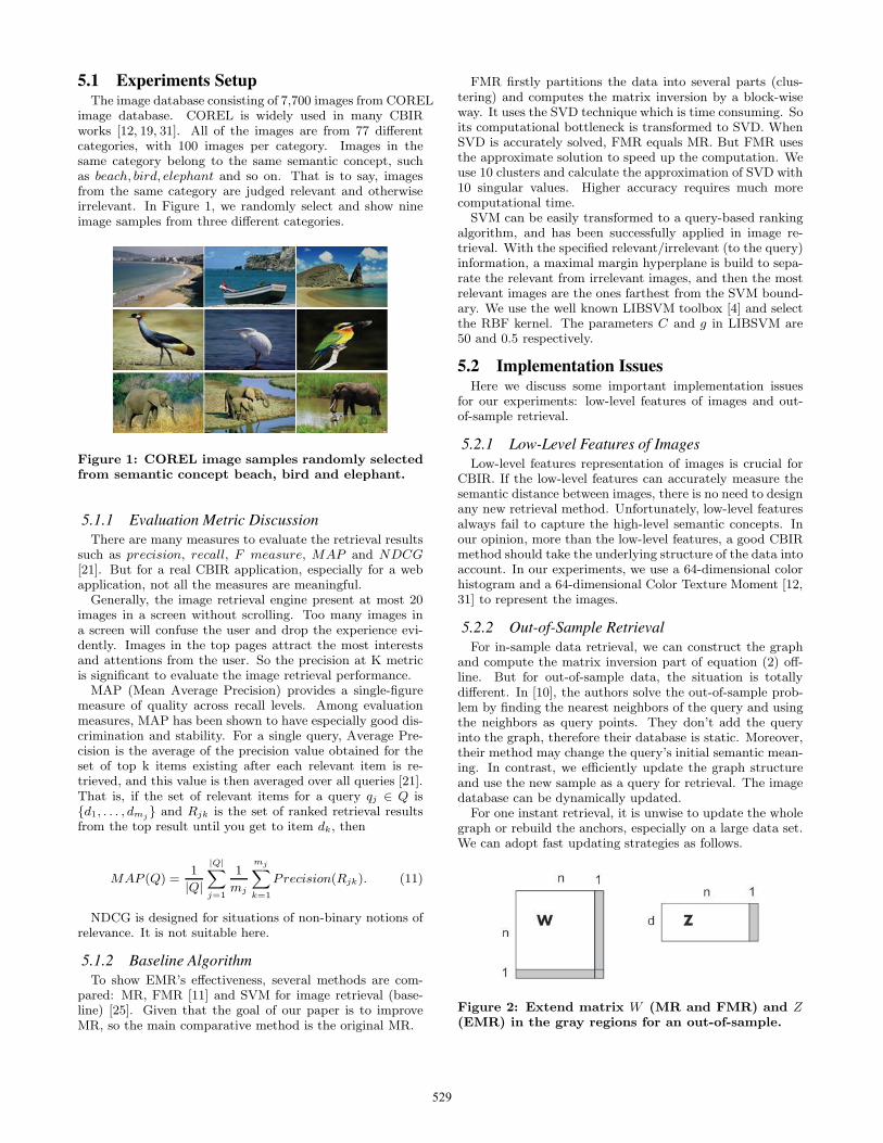
image database. COREL is widely used in many CBIRworks [12, 19, 31]. All of the images are from 77 differentcategories, with 100 images per category. Images in thesame category belong to the same semantic concept, suchas beach, bird, elephant and so on. That is to say, imagesfrom the same category are judged relevant and otherwiseirrelevant. In Figure 1, we randomly select and show nineimage samples from three different categories.

Figure 1: COREL image samples randomly selectedfrom semantic concept beach, bird and elephant.

5.1.1 Evaluation Metric DiscussionThere are many measures to evaluate the retrieval results

such as precision, recall, F measure, MAP and NDCG[21]. But for a real CBIR application, especially for a webapplication, not all the measures are meaningful.

Generally, the image retrieval engine present at most 20images in a screen without scrolling. Too many images ina screen will confuse the user and drop the experience evi-dently. Images in the top pages attract the most interestsand attentions from the user. So the precision at K metricis significant to evaluate the image retrieval performance.

MAP (Mean Average Precision) provides a single-figuremeasure of quality across recall levels. Among evaluationmeasures, MAP has been shown to have especially good dis-crimination and stability. For a single query, Average Pre-cision is the average of the precision value obtained for theset of top k items existing after each relevant item is re-trieved, and this value is then averaged over all queries [21].That is, if the set of relevant items for a query qj ∈ Q is{d1, . . . , dmj} and Rjk is the set of ranked retrieval resultsfrom the top result until you get to item dk, then

MAP (Q) =1

|Q||Q|∑j=1

1

mj

mj∑k=1

Precision(Rjk). (11)

NDCG is designed for situations of non-binary notions ofrelevance. It is not suitable here.

5.1.2 Baseline AlgorithmTo show EMR’s effectiveness, several methods are com-

pared: MR, FMR [11] and SVM for image retrieval (base-line) [25]. Given that the goal of our paper is to improveMR, so the main comparative method is the original MR.

FMR firstly partitions the data into several parts (clus-tering) and computes the matrix inversion by a block-wiseway. It uses the SVD technique which is time consuming. Soits computational bottleneck is transformed to SVD. WhenSVD is accurately solved, FMR equals MR. But FMR usesthe approximate solution to speed up the computation. Weuse 10 clusters and calculate the approximation of SVD with10 singular values. Higher accuracy requires much morecomputational time.

SVM can be easily transformed to a query-based rankingalgorithm, and has been successfully applied in image re-trieval. With the specified relevant/irrelevant (to the query)information, a maximal margin hyperplane is build to sepa-rate the relevant from irrelevant images, and then the mostrelevant images are the ones farthest from the SVM bound-ary. We use the well known LIBSVM toolbox [4] and selectthe RBF kernel. The parameters C and g in LIBSVM are50 and 0.5 respectively.

5.2 Implementation IssuesHere we discuss some important implementation issues

for our experiments: low-level features of images and out-of-sample retrieval.

5.2.1 Low-Level Features of ImagesLow-level features representation of images is crucial for

CBIR. If the low-level features can accurately measure thesemantic distance between images, there is no need to designany new retrieval method. Unfortunately, low-level featuresalways fail to capture the high-level semantic concepts. Inour opinion, more than the low-level features, a good CBIRmethod should take the underlying structure of the data intoaccount. In our experiments, we use a 64-dimensional colorhistogram and a 64-dimensional Color Texture Moment [12,31] to represent the images.

5.2.2 Out-of-Sample RetrievalFor in-sample data retrieval, we can construct the graph

and compute the matrix inversion part of equation (2) off-line. But for out-of-sample data, the situation is totallydifferent. In [10], the authors solve the out-of-sample prob-lem by finding the nearest neighbors of the query and usingthe neighbors as query points. They don’t add the queryinto the graph, therefore their database is static. Moreover,their method may change the query’s initial semantic mean-ing. In contrast, we efficiently update the graph structureand use the new sample as a query for retrieval. The imagedatabase can be dynamically updated.

For one instant retrieval, it is unwise to update the wholegraph or rebuild the anchors, especially on a large data set.We can adopt fast updating strategies as follows.

Figure 2: Extend matrix W (MR and FMR) and Z(EMR) in the gray regions for an out-of-sample.

529

A fast but inexact strategy for MR and FMR is leavingthe original graph unchanged and adding a new row and anew column toW . But k nearest neighbor relationship is notsymmetric, therefore the query’s neighbors would lose somelocal information – its original neighbors’ weights decreaserelatively and they may have k+1 nearest neighbors. Whilefor EMR, each data point is independently computed. Wejust assign weights between the new query and its nearbyanchors. That forms a new column of Z. One point haslittle effect to the stable anchors in a large data set (e.g.,cluster centers). Figure 2 shows the updating strategies.

5.3 PerformanceWe firstly compare our proposed method EMR with MR,

FMR and baseline on COREL database without relevancefeedback. Relevance feedback asks users to label some re-trieved samples, making the retrieval procedure inconve-nient. So if possible, we prefer an algorithm having goodperformance without relevance feedback. For our methodEMR, 1000 k-means anchors are used. Later in the model se-lection part, we find that using 800 or fewer anchors achievesa close performance.

An important issue needs to be emphasized: although wehave the image labels (categories), we don’t use them inour algorithm, since in real world applications, labeling isvery expensive. The label information can only be used toevaluation and relevance feedback.

At the beginning of the retrieval, we don’t have the userspecified relevant/irrelevant information. To apply SVM,the pseudo relevance feedback [21] strategy, also known asblind relevance feedback is adopted. We rank the images inthe database according to their euclidean distances to thequery, and then the nearest ten images are considered asrelevant and the farthest ten are irrelevant. With such anapproach, we run SVM as normal at the beginning, and theuser gets images without any additional interaction.

5.3.1 Average AccuracyEach image is used as a query and the retrieval perfor-

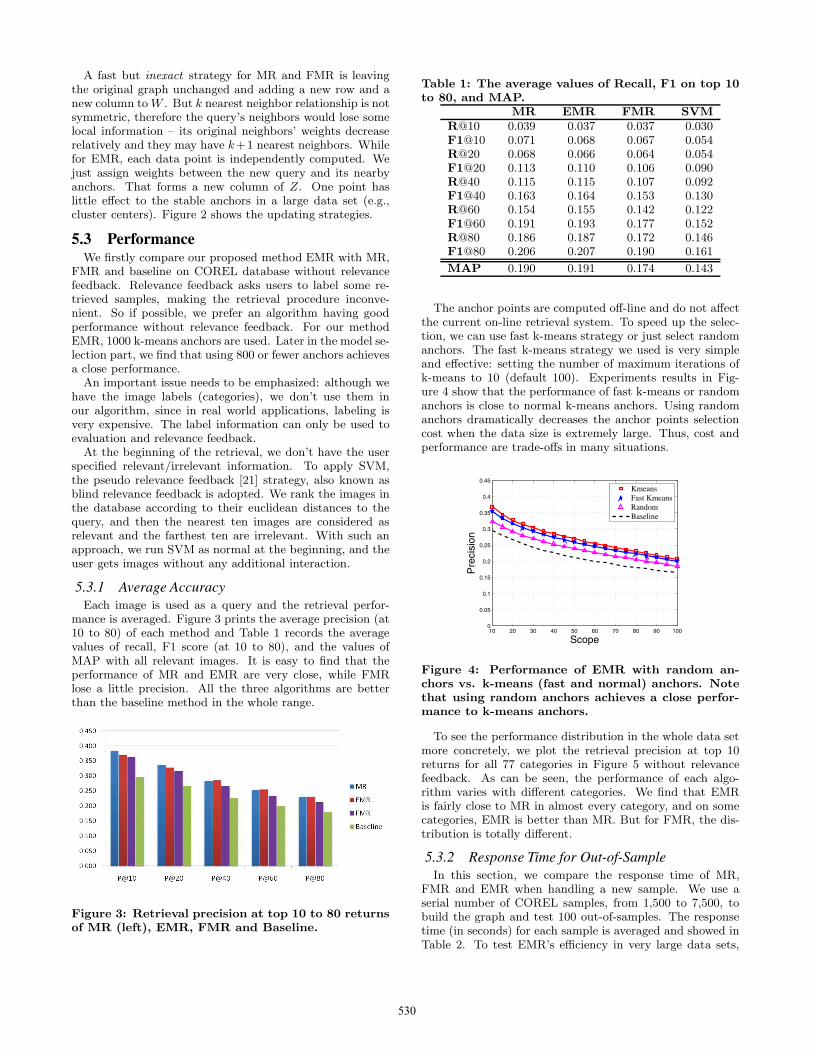
mance is averaged. Figure 3 prints the average precision (at10 to 80) of each method and Table 1 records the averagevalues of recall, F1 score (at 10 to 80), and the values ofMAP with all relevant images. It is easy to find that theperformance of MR and EMR are very close, while FMRlose a little precision. All the three algorithms are betterthan the baseline method in the whole range.

Figure 3: Retrieval precision at top 10 to 80 returnsof MR (left), EMR, FMR and Baseline.

Table 1: The average values of Recall, F1 on top 10to 80, and MAP.

MR EMR FMR SVMR@10 0.039 0.037 0.037 0.030F1@10 0.071 0.068 0.067 0.054R@20 0.068 0.066 0.064 0.054F1@20 0.113 0.110 0.106 0.090R@40 0.115 0.115 0.107 0.092F1@40 0.163 0.164 0.153 0.130R@60 0.154 0.155 0.142 0.122F1@60 0.191 0.193 0.177 0.152R@80 0.186 0.187 0.172 0.146F1@80 0.206 0.207 0.190 0.161

MAP 0.190 0.191 0.174 0.143

The anchor points are computed off-line and do not affectthe current on-line retrieval system. To speed up the selec-tion, we can use fast k-means strategy or just select randomanchors. The fast k-means strategy we used is very simpleand effective: setting the number of maximum iterations ofk-means to 10 (default 100). Experiments results in Fig-ure 4 show that the performance of fast k-means or randomanchors is close to normal k-means anchors. Using randomanchors dramatically decreases the anchor points selectioncost when the data size is extremely large. Thus, cost andperformance are trade-offs in many situations.

10 20 30 40 50 60 70 80 90 1000

0.05

0.1

0.15

0.2

0.25

0.3

0.35

0.4

0.45

Scope

Pre

cisi

on

KmeansFast KmeansRandomBaseline

Figure 4: Performance of EMR with random an-chors vs. k-means (fast and normal) anchors. Notethat using random anchors achieves a close perfor-mance to k-means anchors.

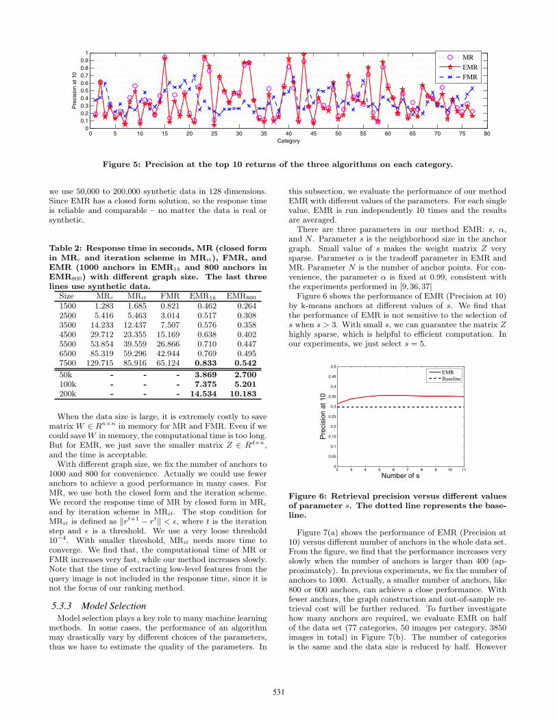
To see the performance distribution in the whole data setmore concretely, we plot the retrieval precision at top 10returns for all 77 categories in Figure 5 without relevancefeedback. As can be seen, the performance of each algo-rithm varies with different categories. We find that EMRis fairly close to MR in almost every category, and on somecategories, EMR is better than MR. But for FMR, the dis-tribution is totally different.

5.3.2 Response Time for Out-of-SampleIn this section, we compare the response time of MR,

FMR and EMR when handling a new sample. We use aserial number of COREL samples, from 1,500 to 7,500, tobuild the graph and test 100 out-of-samples. The responsetime (in seconds) for each sample is averaged and showed inTable 2. To test EMR’s efficiency in very large data sets,

530

0 5 10 15 20 25 30 35 40 45 50 55 60 65 70 75 800

0.10.20.30.40.50.60.70.80.9

1

Category

Pre

cisi

on a

t 10

MR

EMR

FMR

Figure 5: Precision at the top 10 returns of the three algorithms on each category.

we use 50,000 to 200,000 synthetic data in 128 dimensions.Since EMR has a closed form solution, so the response timeis reliable and comparable – no matter the data is real orsynthetic.

Table 2: Response time in seconds, MR (closed formin MRc and iteration scheme in MRit), FMR, andEMR (1000 anchors in EMR1k and 800 anchors inEMR800) with different graph size. The last threelines use synthetic data.

Size MRc MRit FMR EMR1k EMR800

1500 1.283 1.685 0.821 0.462 0.2642500 5.416 5.463 3.014 0.517 0.3083500 14.233 12.437 7.507 0.576 0.3584500 29.712 23.355 15.169 0.638 0.4025500 53.854 39.559 26.866 0.710 0.4476500 85.319 59.296 42.944 0.769 0.4957500 129.715 85.916 65.124 0.833 0.542

50k - - - 3.869 2.700100k - - - 7.375 5.201200k - - - 14.534 10.183

When the data size is large, it is extremely costly to savematrix W ∈ Rn×n in memory for MR and FMR. Even if wecould saveW in memory, the computational time is too long.But for EMR, we just save the smaller matrix Z ∈ Rd×n,and the time is acceptable.

With different graph size, we fix the number of anchors to1000 and 800 for convenience. Actually we could use feweranchors to achieve a good performance in many cases. ForMR, we use both the closed form and the iteration scheme.We record the response time of MR by closed form in MRc

and by iteration scheme in MRit. The stop condition forMRit is defined as ‖rt+1 − rt‖ < ε, where t is the iterationstep and ε is a threshold. We use a very loose threshold10−4. With smaller threshold, MRit needs more time toconverge. We find that, the computational time of MR orFMR increases very fast, while our method increases slowly.Note that the time of extracting low-level features from thequery image is not included in the response time, since it isnot the focus of our ranking method.

5.3.3 Model SelectionModel selection plays a key role to many machine learning

methods. In some cases, the performance of an algorithmmay drastically vary by different choices of the parameters,thus we have to estimate the quality of the parameters. In

this subsection, we evaluate the performance of our methodEMR with different values of the parameters. For each singlevalue, EMR is run independently 10 times and the resultsare averaged.

There are three parameters in our method EMR: s, α,and N . Parameter s is the neighborhood size in the anchorgraph. Small value of s makes the weight matrix Z verysparse. Parameter α is the tradeoff parameter in EMR andMR. Parameter N is the number of anchor points. For con-venience, the parameter α is fixed at 0.99, consistent withthe experiments performed in [9,36,37]

Figure 6 shows the performance of EMR (Precision at 10)by k-means anchors at different values of s. We find thatthe performance of EMR is not sensitive to the selection ofs when s > 3. With small s, we can guarantee the matrix Zhighly sparse, which is helpful to efficient computation. Inour experiments, we just select s = 5.

2 3 4 5 6 7 8 9 10 110

0.05

0.1

0.15

0.2

0.25

0.3

0.35

0.4

0.45

0.5

Number of s

Pre

cisi

on a

t 10

EMRBaseline

Figure 6: Retrieval precision versus different valuesof parameter s. The dotted line represents the base-line.

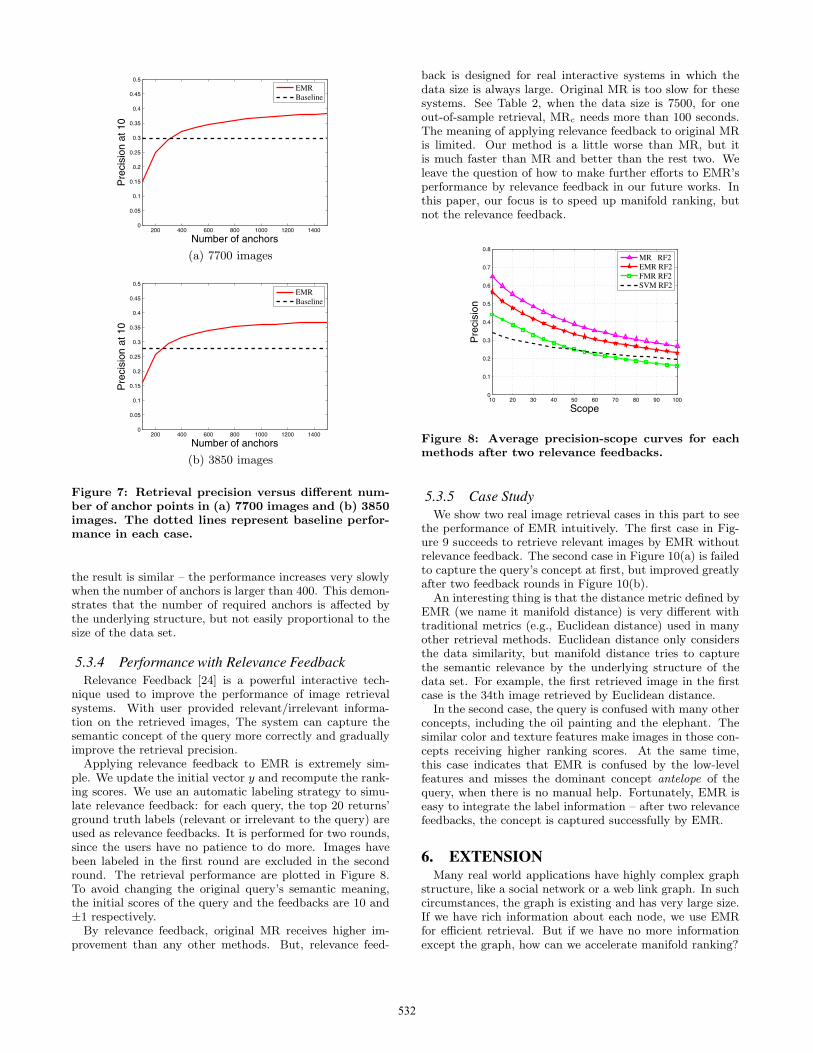
Figure 7(a) shows the performance of EMR (Precision at10) versus different number of anchors in the whole data set.From the figure, we find that the performance increases veryslowly when the number of anchors is larger than 400 (ap-proximately). In previous experiments, we fix the number ofanchors to 1000. Actually, a smaller number of anchors, like800 or 600 anchors, can achieve a close performance. Withfewer anchors, the graph construction and out-of-sample re-trieval cost will be further reduced. To further investigatehow many anchors are required, we evaluate EMR on halfof the data set (77 categories, 50 images per category, 3850images in total) in Figure 7(b). The number of categoriesis the same and the data size is reduced by half. However

531

200 400 600 800 1000 1200 14000

0.05

0.1

0.15

0.2

0.25

0.3

0.35

0.4

0.45

0.5

Number of anchors

Pre

cisi

on a

t 10

EMRBaseline

(a) 7700 images

200 400 600 800 1000 1200 14000

0.05

0.1

0.15

0.2

0.25

0.3

0.35

0.4

0.45

0.5

Number of anchors

Pre

cisi

on a

t 10

EMRBaseline

(b) 3850 images

Figure 7: Retrieval precision versus different num-ber of anchor points in (a) 7700 images and (b) 3850images. The dotted lines represent baseline perfor-mance in each case.

the result is similar – the performance increases very slowlywhen the number of anchors is larger than 400. This demon-strates that the number of required anchors is affected bythe underlying structure, but not easily proportional to thesize of the data set.

5.3.4 Performance with Relevance FeedbackRelevance Feedback [24] is a powerful interactive tech-

nique used to improve the performance of image retrievalsystems. With user provided relevant/irrelevant informa-tion on the retrieved images, The system can capture thesemantic concept of the query more correctly and graduallyimprove the retrieval precision.

Applying relevance feedback to EMR is extremely sim-ple. We update the initial vector y and recompute the rank-ing scores. We use an automatic labeling strategy to simu-late relevance feedback: for each query, the top 20 returns’ground truth labels (relevant or irrelevant to the query) areused as relevance feedbacks. It is performed for two rounds,since the users have no patience to do more. Images havebeen labeled in the first round are excluded in the secondround. The retrieval performance are plotted in Figure 8.To avoid changing the original query’s semantic meaning,the initial scores of the query and the feedbacks are 10 and±1 respectively.

By relevance feedback, original MR receives higher im-provement than any other methods. But, relevance feed-

back is designed for real interactive systems in which thedata size is always large. Original MR is too slow for thesesystems. See Table 2, when the data size is 7500, for oneout-of-sample retrieval, MRc needs more than 100 seconds.The meaning of applying relevance feedback to original MRis limited. Our method is a little worse than MR, but itis much faster than MR and better than the rest two. Weleave the question of how to make further efforts to EMR’sperformance by relevance feedback in our future works. Inthis paper, our focus is to speed up manifold ranking, butnot the relevance feedback.

10 20 30 40 50 60 70 80 90 1000

0.1

0.2

0.3

0.4

0.5

0.6

0.7

0.8

Scope

Pre

cisi

on

MR RF2EMR RF2FMR RF2SVM RF2

Figure 8: Average precision-scope curves for eachmethods after two relevance feedbacks.

5.3.5 Case StudyWe show two real image retrieval cases in this part to see

the performance of EMR intuitively. The first case in Fig-ure 9 succeeds to retrieve relevant images by EMR withoutrelevance feedback. The second case in Figure 10(a) is failedto capture the query’s concept at first, but improved greatlyafter two feedback rounds in Figure 10(b).

An interesting thing is that the distance metric defined byEMR (we name it manifold distance) is very different withtraditional metrics (e.g., Euclidean distance) used in manyother retrieval methods. Euclidean distance only considersthe data similarity, but manifold distance tries to capturethe semantic relevance by the underlying structure of thedata set. For example, the first retrieved image in the firstcase is the 34th image retrieved by Euclidean distance.

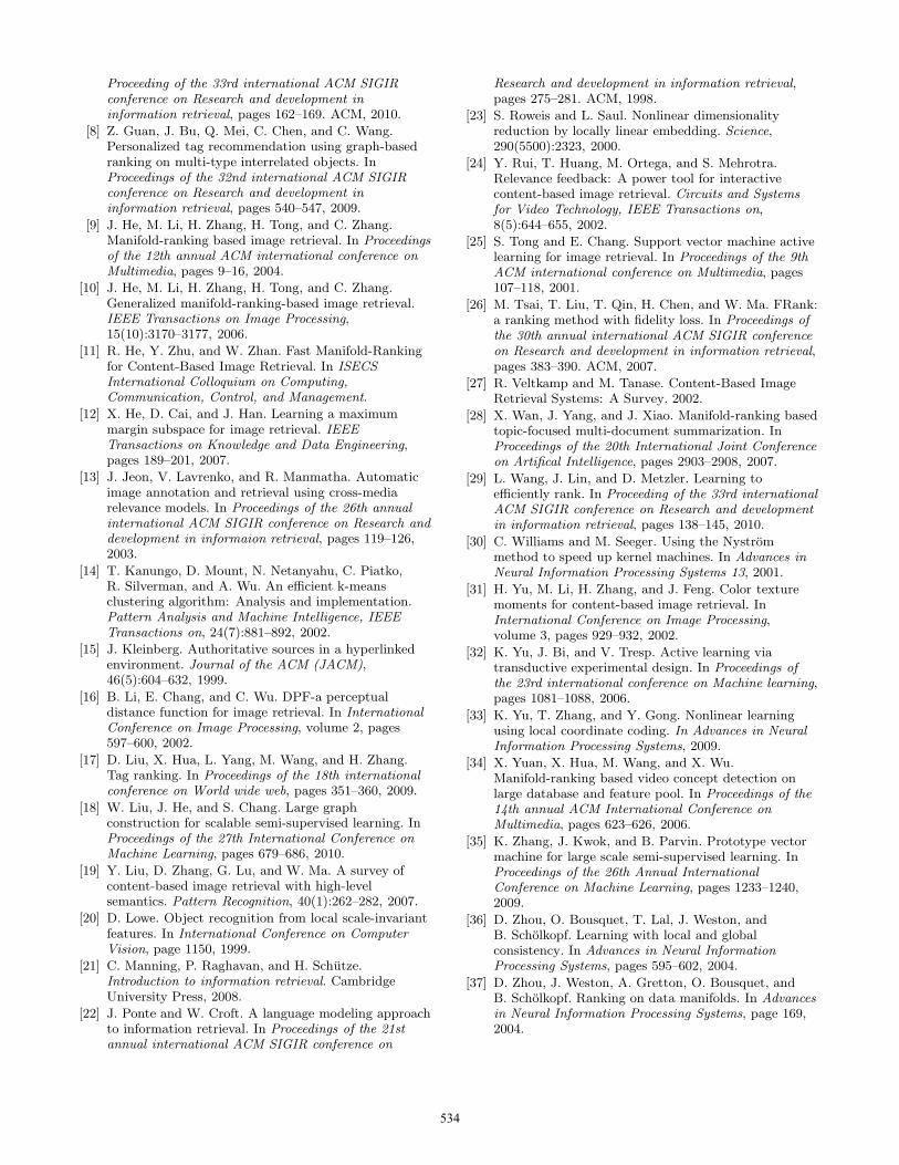
In the second case, the query is confused with many otherconcepts, including the oil painting and the elephant. Thesimilar color and texture features make images in those con-cepts receiving higher ranking scores. At the same time,this case indicates that EMR is confused by the low-levelfeatures and misses the dominant concept antelope of thequery, when there is no manual help. Fortunately, EMR iseasy to integrate the label information – after two relevancefeedbacks, the concept is captured successfully by EMR.

6. EXTENSIONMany real world applications have highly complex graph

structure, like a social network or a web link graph. In suchcircumstances, the graph is existing and has very large size.If we have rich information about each node, we use EMRfor efficient retrieval. But if we have no more informationexcept the graph, how can we accelerate manifold ranking?

532

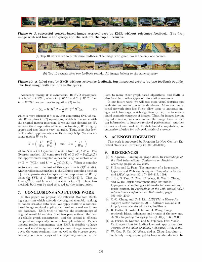
Figure 9: A successful content-based image retrieval case by EMR without relevance feedback. The firstimage with red box is the query, and the rest are the top 10 returns.

(a) Top 10 returns without relevance feedback. The image with green box is the only one correct.

(b) Top 10 returns after two feedback rounds. All images belong to the same category.

Figure 10: A failed case by EMR without relevance feedback, but improved greatly by two feedback rounds.The first image with red box is the query.

Adjacency matrix W is symmetric. Its SVD decomposi-tion is W = UΣUT , where U ∈ Rn×k and Σ ∈ Rk×k. Let

H = D− 12U , we can rewrite equation (2) to be

r∗ = (In −H(HTH − 1

αΣ−1)−1HT )y, (12)

which is very efficient if k n. But computing SVD of ma-trix W requires O(n3) operations, which is the same withthe original matrix inversion. If we can fast decompose W ,we save the computational time. Fortunately, W is highlysparse and may have a very low rank. Thus, some fast low-rank matrix approximation methods may help. We can ar-range matrix W to be

W =

(G W T

21

W21 W22

)and C =

(G

W21

)where G is a l × l symmetric matrix from W , l n. TheNystrom method [30] computes SVD of G (G = UGΣGU

TG )

and approximates singular values and singular vectors of W

by Σ = (nl)ΣG and U =

√lnCUGΣ

−1G . When k singular

vectors are used, the cost of this algorithm is O(l3 + nlk).Another alternative method is the Column-sampling method[6]. It approximates the spectral decomposition of W byusing the SVD of C directly (C = UCΣCV

TC ). That is,

Σ =√

nlΣC and U = UC . Its cost is O(nl2). These two

methods both can be used to speed up the computation.

7. CONCLUSIONS AND FUTURE WORKIn this paper, we propose the Efficient Manifold Rank-

ing algorithm which extends the original manifold rankingto handle scalable data sets. We apply EMR to a content-based image retrieval application based on a real world im-age database. EMR tries to address the shortcomings oforiginal manifold ranking from two perspectives: the firstis scalable graph construction; and the second is efficientcomputation, especially for out-of-sample retrieval. Exper-imental results demonstrate that EMR is feasible to largescale real world image retrieval systems – it significantly re-duces the computational time, as well as the storage space.Actually, our new design of the adjacency matrix can be

used to many other graph-based algorithms, and EMR isalso feasible to other types of information resources.

In our future work, we will test more visual features andevaluate our method on other databases. Moreover, manysocial network sites like Flickr allow users to annotate im-ages with free tags, which significantly help us to under-stand semantic concepts of images. Thus, for images havingtag information, we can combine the image features andtag information to improve retrieval performance. Anotherextension of our work is the distributed computation, anenterprise solution for web scale retrieval systems.

8. ACKNOWLEDGEMENTThis work is supported by Program for New Century Ex-

cellent Talents in University (NCET-09-0685).

9. REFERENCES[1] S. Agarwal. Ranking on graph data. In Proceedings of

the 23rd International Conference on MachineLearning, pages 25–32, 2006.

[2] S. Brin and L. Page. The anatomy of a large-scalehypertextual Web search engine. Computer networksand ISDN systems, 30(1-7):107–117, 1998.

[3] J. Bu, S. Tan, C. Chen, C. Wang, H. Wu, L. Zhang,and X. He. Music recommendation by unifiedhypergraph: combining social media information andmusic content. In Proceedings of the 18th annual ACMinternational conference on Multimedia, pages391–400, 2010.

[4] C.-C. Chang and C.-J. Lin. LIBSVM: a library forsupport vector machines, 2001. Software available athttp://www.csie.ntu.edu.tw/ cjlin/libsvm.

[5] R. Datta, D. Joshi, J. Li, and J. Wang. Imageretrieval: Ideas, influences, and trends of the new age.ACM Computing Surveys (CSUR), 40(2):1–60, 2008.

[6] A. Frieze, R. Kannan, and S. Vempala. Fast MonteCarlo algorithms for finding low-rank approximations.Journal of the ACM (JACM), 51(6):1025–1041, 2004.

[7] W. Gao, P. Cai, K. Wong, and A. Zhou. Learning torank only using training data from related domain. In

533

Proceeding of the 33rd international ACM SIGIRconference on Research and development ininformation retrieval, pages 162–169. ACM, 2010.

[8] Z. Guan, J. Bu, Q. Mei, C. Chen, and C. Wang.Personalized tag recommendation using graph-basedranking on multi-type interrelated objects. InProceedings of the 32nd international ACM SIGIRconference on Research and development ininformation retrieval, pages 540–547, 2009.

[9] J. He, M. Li, H. Zhang, H. Tong, and C. Zhang.Manifold-ranking based image retrieval. In Proceedingsof the 12th annual ACM international conference onMultimedia, pages 9–16, 2004.

[10] J. He, M. Li, H. Zhang, H. Tong, and C. Zhang.Generalized manifold-ranking-based image retrieval.IEEE Transactions on Image Processing,15(10):3170–3177, 2006.

[11] R. He, Y. Zhu, and W. Zhan. Fast Manifold-Rankingfor Content-Based Image Retrieval. In ISECSInternational Colloquium on Computing,Communication, Control, and Management.

[12] X. He, D. Cai, and J. Han. Learning a maximummargin subspace for image retrieval. IEEETransactions on Knowledge and Data Engineering,pages 189–201, 2007.

[13] J. Jeon, V. Lavrenko, and R. Manmatha. Automaticimage annotation and retrieval using cross-mediarelevance models. In Proceedings of the 26th annualinternational ACM SIGIR conference on Research anddevelopment in informaion retrieval, pages 119–126,2003.

[14] T. Kanungo, D. Mount, N. Netanyahu, C. Piatko,R. Silverman, and A. Wu. An efficient k-meansclustering algorithm: Analysis and implementation.Pattern Analysis and Machine Intelligence, IEEETransactions on, 24(7):881–892, 2002.

[15] J. Kleinberg. Authoritative sources in a hyperlinkedenvironment. Journal of the ACM (JACM),46(5):604–632, 1999.

[16] B. Li, E. Chang, and C. Wu. DPF-a perceptualdistance function for image retrieval. In InternationalConference on Image Processing, volume 2, pages597–600, 2002.

[17] D. Liu, X. Hua, L. Yang, M. Wang, and H. Zhang.Tag ranking. In Proceedings of the 18th internationalconference on World wide web, pages 351–360, 2009.

[18] W. Liu, J. He, and S. Chang. Large graphconstruction for scalable semi-supervised learning. InProceedings of the 27th International Conference onMachine Learning, pages 679–686, 2010.

[19] Y. Liu, D. Zhang, G. Lu, and W. Ma. A survey ofcontent-based image retrieval with high-levelsemantics. Pattern Recognition, 40(1):262–282, 2007.

[20] D. Lowe. Object recognition from local scale-invariantfeatures. In International Conference on ComputerVision, page 1150, 1999.

[21] C. Manning, P. Raghavan, and H. Schutze.Introduction to information retrieval. CambridgeUniversity Press, 2008.

[22] J. Ponte and W. Croft. A language modeling approachto information retrieval. In Proceedings of the 21stannual international ACM SIGIR conference on

Research and development in information retrieval,pages 275–281. ACM, 1998.

[23] S. Roweis and L. Saul. Nonlinear dimensionalityreduction by locally linear embedding. Science,290(5500):2323, 2000.

[24] Y. Rui, T. Huang, M. Ortega, and S. Mehrotra.Relevance feedback: A power tool for interactivecontent-based image retrieval. Circuits and Systemsfor Video Technology, IEEE Transactions on,8(5):644–655, 2002.

[25] S. Tong and E. Chang. Support vector machine activelearning for image retrieval. In Proceedings of the 9thACM international conference on Multimedia, pages107–118, 2001.

[26] M. Tsai, T. Liu, T. Qin, H. Chen, and W. Ma. FRank:a ranking method with fidelity loss. In Proceedings ofthe 30th annual international ACM SIGIR conferenceon Research and development in information retrieval,pages 383–390. ACM, 2007.

[27] R. Veltkamp and M. Tanase. Content-Based ImageRetrieval Systems: A Survey. 2002.

[28] X. Wan, J. Yang, and J. Xiao. Manifold-ranking basedtopic-focused multi-document summarization. InProceedings of the 20th International Joint Conferenceon Artifical Intelligence, pages 2903–2908, 2007.

[29] L. Wang, J. Lin, and D. Metzler. Learning toefficiently rank. In Proceeding of the 33rd internationalACM SIGIR conference on Research and developmentin information retrieval, pages 138–145, 2010.

[30] C. Williams and M. Seeger. Using the Nystrommethod to speed up kernel machines. In Advances inNeural Information Processing Systems 13, 2001.

[31] H. Yu, M. Li, H. Zhang, and J. Feng. Color texturemoments for content-based image retrieval. InInternational Conference on Image Processing,volume 3, pages 929–932, 2002.

[32] K. Yu, J. Bi, and V. Tresp. Active learning viatransductive experimental design. In Proceedings ofthe 23rd international conference on Machine learning,pages 1081–1088, 2006.

[33] K. Yu, T. Zhang, and Y. Gong. Nonlinear learningusing local coordinate coding. In Advances in NeuralInformation Processing Systems, 2009.

[34] X. Yuan, X. Hua, M. Wang, and X. Wu.Manifold-ranking based video concept detection onlarge database and feature pool. In Proceedings of the14th annual ACM International Conference onMultimedia, pages 623–626, 2006.

[35] K. Zhang, J. Kwok, and B. Parvin. Prototype vectormachine for large scale semi-supervised learning. InProceedings of the 26th Annual InternationalConference on Machine Learning, pages 1233–1240,2009.

[36] D. Zhou, O. Bousquet, T. Lal, J. Weston, andB. Scholkopf. Learning with local and globalconsistency. In Advances in Neural InformationProcessing Systems, pages 595–602, 2004.

[37] D. Zhou, J. Weston, A. Gretton, O. Bousquet, andB. Scholkopf. Ranking on data manifolds. In Advancesin Neural Information Processing Systems, page 169,2004.

534