Embed Size (px)
Citation preview
General rights Copyright and moral rights for the publications made accessible in the public portal are retained by the authors and/or other copyright owners and it is a condition of accessing publications that users recognise and abide by the legal requirements associated with these rights.
Users may download and print one copy of any publication from the public portal for the purpose of private study or research.
You may not further distribute the material or use it for any profit-making activity or commercial gain
You may freely distribute the URL identifying the publication in the public portal If you believe that this document breaches copyright please contact us providing details, and we will remove access to the work immediately and investigate your claim.
Downloaded from orbit.dtu.dk on: Feb 15, 2019
Few-photon Non-linearities in Nanophotonic Devices for Quantum InformationTechnology
Nysteen, Anders; Mørk, Jesper; Kristensen, Philip Trøst; McCutcheon, Dara; Nielsen, Per Kær
Publication date:2015
Document VersionPublisher's PDF, also known as Version of record
Link back to DTU Orbit
Citation (APA):Nysteen, A., Mørk, J., Kristensen, P. T., McCutcheon, D., & Nielsen, P. K. (2015). Few-photon Non-linearities inNanophotonic Devices for Quantum Information Technology. Technical University of Denmark (DTU).
Few-photon Non-linearities in
Nanophotonic Devices for
Quantum Information Technology
A dissertationsubmitted to the Department of Photonics Engineering
at the Technical University of Denmarkin partial fulfillment of the requirements
for the degree ofphilosophiae doctor
Anders NysteenMarch 14, 2015
DTU FotonikDepartment of Photonics Engineering
Technical University of Denmark

Few-photon Non-linearities in
Nanophotonic Devices for
Quantum Information Technology

Preface
This thesis is submitted in candidacy for the PhD degree from the TechnicalUniversity of Denmark. The research has been carried out in the NanophotonicsTheory and Signal Processing Group at DTU Fotonik - Department of Photon-ics Engineering from 2012-2015, under the supervision of Jesper Mørk, PhilipT. Kristensen, Dara P. S. McCutcheon, and Per Kær Nielsen. In July-October2014 I visited the Quantum Photonics Group at Massachusetts Institute ofTechnology lead by Prof. Dirk Englund. The main purpose of the visit was toadd an experimental point of view to the structures considered in this thesisand to discuss possible implementations of few-photon non-linearities.
Acknowledgements
First and foremost I would like to thank my great team of supervisors: JesperMørk, Dara P. S. McCutcheon, Philip Trøst Kristensen, and Per Kær Nielsen.Jesper has been following my studies since 2009, and as my main supervisorduring my PhD studies and in several smaller projects, Jesper has providedvaluable supervision and encouraging input to the projects with his enormousphysical insight. Philip, Per, and Dara have all contributed to different stagesof the PhD studies with their solid knowledge of both theoretical and numericalmethods, and I valued every discussion we had during the project.
I would like to thank Dirk Englund and Mikkel Heuck for making it possi-ble for me to spend three months in the Quantum Photonics Group at MIT,allowing me to get an great experimental point of view to my research. I alsowish to express my gratitude towards the Quantum Photonics Group at theNiels Bohr Institute, especially Peter Lodahl, Kristian H. Madsen and AsgerKreiner-Møller for fruitful discussions about electron-phonon interaction andfor carrying out the experimental measurements of phonon-effects in a coupledquantum dot–optical cavity system. Additionally I would like to thank ImmoSöllner, Sahand Mahmoodian and Marta Arcari for sharing their insight on theimplementation of quantum dot non-linearities in photonic crystal systems.
Furthermore, I would like to thank the entire Nanophotonics Theory andSignal Processing Group, especially my old office mate Anders Lund, and ofcourse also to my two study-buddies Lasse Andersen and Mikkel Settnes, whomI have worked with throughout all of my years of study. Finally, I would liketo give special thanks to my family, friends and my girlfriend for supportingme throughout this project.
iii

AbstractIn this thesis we investigate few-photon non-linearities in all-optical, on-chipcircuits, and we discuss their possible applications in devices of interest forquantum information technology, such as conditional two-photon gates andsingle-photon sources.
In order to propose efficient devices, it is crucial to fully understand thenon-equilibrium dynamics of strongly interacting photons. Employing bothnumerical and analytical approaches we map out the full scattering dynamicsfor two photons scattering on a two-level emitter in a one-dimensional waveg-uide. The strongest non-linear interaction arise when the emitter is excitedthe most, which occurs for incoming photon pulses with a spectral bandwidthcomparable to the emitter linewidth. For two identical, counter-propagatingphotons, the emitter works as a non-linear beam splitter, as the emitter inducesstrong directional correlations between the scattered photons. Even though thenon-linearity also alters the pulse spectrum due to a four-wave mixing process,we demonstrate that input pulses with a Gaussian spectrum can be mapped tothe output with up to 80 % fidelity.
Using two identical two-level emitters, we propose a setup for a deterministiccontrolled-phase gate, which preserves the properties of the two incoming pho-tons with almost 80 %, limited by spectral changes induced by the non-linearityand phase modulations upon scattering. Another setup for a controlled-phaseoperation is suggested with two coupled ring resonators exploiting a strongsecond-order material non-linearity. By dynamically trapping the first of twotemporally separated photons in the non-linear resonator, the scattering of thesecond photon is altered. Due to the trapping, the undesired aforementionednon-linear effects are avoided, but the gate performance is now limited by thecapturing process.
Semiconductor quantum dots (QDs) are promising for realizing few-photonnon-linearities in solid-state implementations, although coupling to phononmodes in the surrounding lattice have significant influence on the dynamics.By accounting for the commonly neglected asymmetry between the electronand hole wavefunction in the QD, we show how the phonon-assisted transitionrate to a slightly detuned optical mode may be suppressed. This is achievedby properly matching the electrical carrier confinement with the deformationpotential interaction, where the suppression only occurs in materials where thedeformation potential interaction shifts the electron and hole bands in the samedirection. We demonstrate also how the phonon-induced effects may be alteredby placing the QD inside an infinite slab, where the confinement of the phononsis modified instead. For a slab thickness below ∼ 70 nm, the bulk description
v
of the phonon modes may be insufficient. The QD decay rate may be stronglyincreased or decreased, depending on how the detuning between the QD andthe optical mode matches the phonon modes in the slab.
Anders Nysteen February 14th, 2015
vi
ResuméI denne afhandling undersøges få-foton ikke-lineariteter i integrerede optiskekredsløb, og vi diskuterer muligheder for at anvende ikke-lineariteterne i kom-ponenter til kvanteinformatik, såsom betingede to-foton–porte og enkeltfo-tonkilder.
For at kunne foreslå effektive komponenter er det vigtigt at forstå ikke-ligevægtsdynamikken for stærkt vekselvirkende fotoner fuldt ud. Ved at benyttebåde numeriske og analytiske tilgange beskriver vi den fulde spredningsdy-namik for to fotoner, der spreder på en to-niveau-emitter i en en-dimensionelbølgeleder. Den største interaktion opnås, når emitteren er mest eksiteret,hvilket sker når de indkomne foton-pulser har en spektral linjebredde i sammestørrelsesorden som emitterens. For to identiske, mod-propagerende fotonerfungerer emitteren som en ikke-lineær beam-splitter, idet emitteren inducererstærke korrelationer imellem de to fotoners spredningsretning. Selvom ikke-lineariteten også ændrer fotonernes spektrum på grund af fire-bølge-blanding,da vil indkomne pulse med et Gaussisk spektrum blive mappet til output-portenmed helt op til næsten 80 % fidelity.
Ved at benytte to identiske to-niveau emittere foreslår vi et setup for en de-terministisk kontrolleret fase-port, som bevarer egenskaberne af de to indkomnefotoner med næsten 80 %, begrænset af spektrale ændringer induceret af ikke-lineariteten og fasemodulationer ved spredningen. Vi foreslår også et andetsetup til en kontrolleret fase-port, som består af to koblede ring-resonatorersom har en kraftig anden-ordens materiale-ikke-linearitet. Ved dynamisk atfange den første af de to tidsligt adskildte fotoner i den ikke-lineære resonator,vil spredningen af den anden foton påvirkes. Ved denne dynamiske indfangsme-tode undgås de omtalte uønskede effekter fra ikke-lineariteterne, men i stedetvil effektiviteten af porten være begrænset af usikkerhederne ved den dynamiskeindfangningsproces.
Halvleder kvantepunkter er lovende kandidater i realiseringen af enkelt-foton ikke-lineariteter i faststof-implementationer, selvom kobling til fonon-tilstande i det omkringliggende gitter kan have stor indflydelse på dynamikken.Ved at tage højde for den typisk ignorerede asymmetri imellem elektron- oghulbølgefunktionen i kvantepunktet viser vi, hvordan den fonon-assisteredeovergangsrate til en nær-resonant optisk tilstand kan blive undertrykt. Detteopnås ved at tilpasse begrænsningen af de elektroniske ladningsbærere meddeformationspotentiale-interaktionen, og denne undertrykkelse finder kun stedi materialer hvor deformationspotentiale-interaktionen rykker elektron og hul-bånd i samme retning. Vi demonstrerer også, hvordan fonon-inducerede ef-fekter kan ændres ved at placere kvantepunktet inden i en uendelig plade,
vii
hvor begrænsningen af fononerne i stedet er ændret. For pladetykkelser un-der ∼ 70 nm vil beskrivelsen af fononerne som rumligt ubegrænsede ikke væretilstrækkelig længere. I det tilfælde vil henfaldsraten af kvantepunktet kunnevære både stærkt øget eller formindsket, afhængig af hvordan energiforskellenimellem kvantedotten og den optiske tilstand matcher med fonon-tilstandene iden uendelige plade.
viii
List of Publications
Journal publications
1. A. Nysteen, P. T. Kristensen, D. P. S. McCutcheon, P. Kaer, and J. Mørk.Scattering of two photons on a quantum emitter in a one-dimensionalwaveguide: exact dynamics and induced correlations. New Jour. Phys.17, 023030 (2015)
2. K. H. Madsen, P. K. Nielsen, A. Kreiner-Møller, S. Stobbe, A. Nysteen,J. Mørk, and P. Lodahl. Measuring the effective phonon density of statesof a quantum dot in cavity quantum electrodynamics. Phys. Rev. B 88,045316 (2013).
3. A. Nysteen, P. K. Nielsen, and J. Mørk. Proposed Quenching of Phonon-Induced Processes in Photoexcited Quantum Dots due to Electron-HoleAsymmetries. Phys. Rev. Lett. 110, 087401 (2013).
4. A. Nysteen, P. K. Nielsen, and J. Mørk. Reducing dephasing in cou-pled quantum dot-cavity systems by engineering the carrier wavefunctions.Proceedings of SPIE, the International Society for Optical Engineering8271, 82710E (2012)
Submitted manuscripts
1. A. Nysteen, D. P. S. McCutcheon, and J. Mørk. Strong non-linearity-induced correlations for counter-propagating photons scattering on a two-level emitter. arXiv:1502.04729 (2015).
Conference contributions
1. K. H. Madsen, P. K. Nielsen, A. Kreiner-Møller, S. Stobbe, A. Nysteen,J. Mørk, and P. Lodahl. Measuring the effective phonon density of statesof a quantum dot. International Conference on Optics of Excitons inConfined Systems (OECS13) Rome, Italy (2013).
2. K. H. Madsen, P. K. Nielsen, A. Kreiner-Møller, S. Stobbe, A. Nysteen,J. Mørk, and P. Lodahl. Non-Markovian phonon dephasing of a quan-tum dot in a photonic-crystal nanocavity. 11th International Workshopon Nonlinear Optics and Excitation Kinetics in Semiconductors, p. 82(2012).
ix
3. A. Nysteen, P. K. Nielsen, and J. Mørk. Suppressing electron-phononinteractions in semiconductor quantum dot systems by engineering theelectronic wavefunctions. 11th International Workshop on Nonlinear Op-tics and Excitation Kinetics in Semiconductors, p. 64 (2012).
ii
Contents
1 Introduction 1
1.1 Few-photon non-linearities . . . . . . . . . . . . . . . . . . . . . 21.2 All-optical integrated circuits . . . . . . . . . . . . . . . . . . . 31.3 Thesis outline . . . . . . . . . . . . . . . . . . . . . . . . . . . . 4
2 Governing Hamiltonians 7
2.1 Many-body Hamiltonian . . . . . . . . . . . . . . . . . . . . . . 7
3 Single-photon scattering 15
3.1 The model . . . . . . . . . . . . . . . . . . . . . . . . . . . . . . 173.2 A single system excitation . . . . . . . . . . . . . . . . . . . . . 18
3.2.1 Input state . . . . . . . . . . . . . . . . . . . . . . . . . 193.2.2 Dynamics . . . . . . . . . . . . . . . . . . . . . . . . . . 20
3.3 Numerical Implementation . . . . . . . . . . . . . . . . . . . . . 233.4 Summary . . . . . . . . . . . . . . . . . . . . . . . . . . . . . . 25
4 Two-photon scattering — Wavefunction approach 27
4.1 Introduction . . . . . . . . . . . . . . . . . . . . . . . . . . . . . 274.2 Two-excitation model . . . . . . . . . . . . . . . . . . . . . . . 28
4.2.1 Two-photon input state . . . . . . . . . . . . . . . . . . 294.3 Co-propagating pulses . . . . . . . . . . . . . . . . . . . . . . . 32
4.3.1 Scattering dynamics . . . . . . . . . . . . . . . . . . . . 334.3.2 Transmission and reflection properties . . . . . . . . . . 36
4.4 Counter-propagating pulses . . . . . . . . . . . . . . . . . . . . 384.4.1 Induced correlations . . . . . . . . . . . . . . . . . . . . 38
4.5 Summary . . . . . . . . . . . . . . . . . . . . . . . . . . . . . . 42
5 Two-photon scattering — Scattering matrix approach 43
5.1 General theory . . . . . . . . . . . . . . . . . . . . . . . . . . . 455.2 Single-photon scattering . . . . . . . . . . . . . . . . . . . . . . 46
5.2.1 Scattering fidelities . . . . . . . . . . . . . . . . . . . . . 475.3 Two-photon scattering . . . . . . . . . . . . . . . . . . . . . . . 49
5.3.1 Two-level emitter . . . . . . . . . . . . . . . . . . . . . . 525.3.2 Scattering fidelities . . . . . . . . . . . . . . . . . . . . . 54
5.4 Summary . . . . . . . . . . . . . . . . . . . . . . . . . . . . . . 57
iii
CONTENTS
6 Controlled phase gate 59
6.1 The controlled phase gate . . . . . . . . . . . . . . . . . . . . . 606.1.1 Gate components . . . . . . . . . . . . . . . . . . . . . . 61
6.2 Gate setup . . . . . . . . . . . . . . . . . . . . . . . . . . . . . 636.2.1 Linear gate interactions . . . . . . . . . . . . . . . . . . 646.2.2 Non-linear gate interactions . . . . . . . . . . . . . . . . 66
6.3 Summary . . . . . . . . . . . . . . . . . . . . . . . . . . . . . . 68
7 Controlled phase gate - Using dynamical capture 71
7.1 Requirements for ring-resonator non-linearity . . . . . . . . . . 737.2 Dynamical capture . . . . . . . . . . . . . . . . . . . . . . . . . 77
7.2.1 Capture and release of the control photon . . . . . . . . 777.2.2 Scattering of the signal photon . . . . . . . . . . . . . . 81
7.3 Summary . . . . . . . . . . . . . . . . . . . . . . . . . . . . . . 83
8 Phonon-induced dynamics — Basic theory 85
8.1 Electron-phonon coupling mechanisms . . . . . . . . . . . . . . 868.1.1 Deformation potential . . . . . . . . . . . . . . . . . . . 87
8.2 Open quantum systems . . . . . . . . . . . . . . . . . . . . . . 898.2.1 The Born-Markov approximation . . . . . . . . . . . . . 90
8.3 Summary . . . . . . . . . . . . . . . . . . . . . . . . . . . . . . 93
9 Phonon-induced dynamics — The electronic confinement 95
9.1 Photoluminescence excitation . . . . . . . . . . . . . . . . . . . 969.2 Coupled QD–cavity system . . . . . . . . . . . . . . . . . . . . 999.3 Experimental investigation . . . . . . . . . . . . . . . . . . . . . 1059.4 Summary . . . . . . . . . . . . . . . . . . . . . . . . . . . . . . 106
10 Phonon-induced dynamics — The phononic confinement 109
10.1 Phonon modes in an infinite slab . . . . . . . . . . . . . . . . . 11010.2 Dynamics . . . . . . . . . . . . . . . . . . . . . . . . . . . . . . 11310.3 Summary . . . . . . . . . . . . . . . . . . . . . . . . . . . . . . 115
11 Highlights and outlook 117
Appendix 123
A Analytical derivation of two-photon emitter excitation 123
A.1 Example: Single-sided Gaussian two-photon input . . . . . . . 130
B Numerical Implementation of wavefunction approach 135
B.1 Single excitation . . . . . . . . . . . . . . . . . . . . . . . . . . 135B.2 Two excitations . . . . . . . . . . . . . . . . . . . . . . . . . . . 136
C Parameters for phonon calculations 139
Bibliography 141
iv
Chapter 1
Introduction
The fundamentals of quantum mechanics were developed in the beginning ofthe 20th century in an attempt to explain the spectral properties of thermal ra-diation, as none of the current theories were sufficient. The first model that wasable to explain experimental results was proposed by Max Planck, by assumingthat the thermal radiation was in equilibrium with a set of harmonic oscillatorswith discrete energy levels [1]. Albert Einstein followed up by claiming thata beam of light actually consists of individual packets, which were later to becalled photons [2]. This quantization of the light lead to major discussions ofthe particle-wave duality of light, but it were also able to explain a yet un-resolved problem regarding interaction between light and matter, namely thephotoelectric effect. These early achievements form the basis of a quantummechanical description of the world with a fundamentally probabilistic nature,where a single particle has a probability of being in one of multiple states at agiven time, in a quantum superposition. And where multiple particles may bein a quantum state where each particle cannot be described independently asthey are quantum mechanically entangled.
This quantum mechanical understanding of the fundamental interaction be-tween light and matter has been of crucial importance in the development ofseveral important components in our daily life such as lasers, diodes, and mag-netic resonance imaging. Quantum mechanics also paves the way for a newera in computational schemes, which has been a hot topic in the last coupleof decades [3]. New functionalities have been made possible by encoding infor-mation into quantum mechanical superpositions called quantum bits (qubits).In contrast to classical bits are is in one of two states at a specific time, thequantum mechanical nature of qubits may be in a superposition of each bitstate at the same time until the state of the qubit is measured.
This relatively new field of quantum information technology promises securecommunication by quantum cryptography [4, 5, 6]. The quantum encoding alsoallows new computational algorithms in the field of quantum computation [3],which promise exponentially faster operation times for specific tasks such assearching databases and factorizing, with the latter having been demonstratedexperimentally by an implementation of Shor’s algorithm [7].
1
Chapter 1. Introduction
In order to realize quantum circuits and quantum networks [8, 9, 10], pho-tons are promising candidates as carriers of the quantum-encoded information[11]. As flying qubits, the information carried in the photons is not easily af-fected by the surrounding environment due to the non-interacting nature of thephotons. The qubit states may be encoded in various degrees of freedom, forexample polarisation states, temporal displacements, and spatial modes (suchas the dual-rail representation) etc. [12, 13].
Realizations of the quantum computation schemes rely on the possibilityof initializing, processing/interacting and measuring qubits efficiently, but asphotons do not mutually interact due to their bosonic nature, advanced ap-proaches must be employed. Using only linear optical elements such as beamsplitters, phase shifters and mirrors, Knill, Laflamme, and Milburn demon-strated in 2001 that it was possible to do quantum computation using single-photon sources and photo-detectors [14]. This so-called KLM scheme exploitsfeedback from the detectors and use several ancilla photons. Suggestions for ef-ficient non-linear gates are proposed, but they are all probabilistic as they onlywork successfully when a specific combination of detection events is obtainedin ancillary arms. This results in scalability-issues when employing multiplegates, although this may be dealt with using quantum teleportation [15]. Ex-perimental implementations of these probabilistic gates have been carried outwith high success rates [16].
1.1 Few-photon non-linearities
In contrast to the probabilistic KLM-scheme, which uses several ancillary pho-tons and detectors, few-photon non-linearities [17] open up for possibilites ofcreating deterministic gate structures without additional ancillary photons anddetectors. Material non-linearities such as the Kerr effect is one example, wherethe photon interaction stems from induced changes in the refractive material.It is, however, an ongoing challenge to find materials with a sufficient non-linearcoefficient in order to work in the single-photon regime. For this, single atomsprove viable candidates as few-photon non-linearities due to their discrete en-ergy levels. These few-photon non-linearities are also existing in so-called ”arti-ficial atoms” such as semiconductor quantum dots (QDs) [18, 19, 20], nitrogenvacancy (NV) centres in diamonds [21, 22], or superconducting circuits [23],which are all physical objects with bound, discrete electronic states.
The atom–light interaction in these systems may be enhanced by placingthe emitter inside an optical cavity, such that the light passes through theatom repediatly. If the rate at which energy oscillates between the atom andthe cavity modes exceeds loss of excitation in the system to external reser-voirs, the atom–cavity system is said to be in the strong coupling regime [24].In this regime, the atom dresses the energy levels of the optical cavity to anan-harmonic energy ladder. Thus, for an incoming beam of photons matchingthe lowest energy level of the dressed state, the strong atom–cavity couplingonly allows a single electron to couple through the cavity at a time – an effectknown as the photon blockade. Experimental demonstrations of this possibilityof controlling the reflectivity of a cavity with a single atom have been carried
2
All-optical integrated circuits
out e.g. by trapping Caesium atoms in a Fabry–Perot cavity [25]. The con-tinuous improvement of micro- and nanofabrication allows precise control ofthe electronic and electromagnetic confinement, and has made it possible toobserve strong coupling even in solid-state system, with a QD coupling to aphotonic crystal cavity [26, 27].
1.2 All-optical integrated circuits
There is currently a great deal of interest on schemes that integrate photonicgates and non-linearities together with photon sources and detectors, on asingle on-chip platform in an all-optical circuit [28, 29, 30]. As the quantumschemes rely on minimal decoherence and losses of the information, it is of highimportance to minimize the losses caused by coupling the different functional-ities together. Coupling losses may be minimized by integrating photon cre-ation, processing and detection on-chip [31]. Promising single-photon sourceshave been demonstrated using QDs in nanowires and photonic crystal cavities[32, 33], and several designs for efficient few-photon detection exist, e.g. usingsuperconducting nanowires [34, 35, 36, 37]
For processing, both single- and two-photon gates are required to make aquantum computer [3, 38], and finding efficient conditional two-photon gates isstill a pressing challenge. Here few-photon non-linearities are promising candi-dates, and demonstrations of several gate functionalities have been developed.By externally changing the state of an atom trapped in the proximity of an op-tical cavity, the scattering direction/phase of a signal beam through the cavitymay be controlled solely by whether the single atom is able to couple the thecavity or not [39, 40]. Alternatively, by trapping single photons or using multi-level emitters, it is possible to switch a multi-photon beam with only a singlecontrol excitation [41, 42, 43]. The dressed cavity–QD system may also be em-ployed in conditional gates for two impinging single-photons of different color,due to the anharmonic energy ladder of the dressed cavity [44]. The structuresmentioned above are all viable candidates for conditional phase gates, but theyall rely on external manipulations to trap atoms or photons or to manipulatethe state of the atom.
Solid-state implementations of the non-linearities such as QDs have beendemonstrated to couple with very high efficiency to confined propagating pho-ton modes [45], and they are promising candidates for on-chip integrated non-linearities. However, the solid state implementation also introduce decoherencedue to coupling between the electrical carriers and the vibrational modes in thesolid-state environment, with the latter being quantized as phonons. When ex-citing a QD optically, acoustic phonons may assist in the coupling and enhancethe coupling rate [46, 47, 48]. The phonons do, however, also introduce dephas-ing, which e.g. in a single-photon source would decrease the indistinguishabilityof the emitter photons [49].
The main purpose of this thesis is to investigate the possibility of integrat-ing the non-linearities and functionalities in an all-optical, deterministic on-chipconfiguration, with a specific focus on the few-photon non-linear processes. In
3
Chapter 1. Introduction
order to propose efficient structures, it is crucial to understand the non-trivialdynamics of strongly interacting photons fully. Using both numerical and ana-lytical approaches we map out the non-linearity-induced correlations in detail,and we discuss how the non-linearity may be exploited in deterministic quan-tum gates. By treating the electron-phonon interaction as a non-Markoviancoupling to a large phonon bath, we examine in detail how both the electronicand phononic confinement affect the dynamics related to the QD. We describehow the confinement of both the electrical carriers and the phonons may beengineered in order to optimize the performance of the quantum systems.
1.3 Thesis outline
In Chapter 2 the governing Hamiltonians are introduced by specifically con-sidering the individual contributions from the different particles present in aquantum system and their mutual interaction.
Chapter 3 treats scattering of a single-photon wavepacket on a two-levelemitter in a one-dimensional waveguide. We describe the fundamental theory ofsingle-photon scattering, with focus on the emitter dynamics and the propertiesof the scattered state. Additionally we introduce a numerical approach todetermine the dynamics of photon scattering in waveguide systems interactingwith localized scatterers in general.
We perform a full numerical calculation of the scattering of two-photonpulses on a two-level emitter in Chapter 4. From the numerics we are ablemap out the full scattering dynamics. Specifically we demonstrate that for twoinitially counter-propagating photons, the emitter acts like a non-linear beamsplitter by imposing strong directional correlations in the scattered state. Thisonly occurs when the bandwidths of the incoming pulses are identical to theemitter linewidth, as the emitter is excited the most in this pulse regime.
In Chapter 5 we exploit the scattering matrix formalism to determine an-alytical expressions for the post-scattering state in Chapter 4. The analyticalapproach allows us to investigate the correlations in the scattered state that arespecifically caused by the emitter non-linearity. Fidelity measurements are in-troduced to describe the scattering-induced correlations, which may take boththe photon spectrum, phase and propagating direction into account. For thecase of two counter-propagating photons, the fidelity of the non-linear beamsplitter is almost 80 %, even when taking all scattering-induced changes in thespectrum and phase of the photons into account.
We discuss direct exploitation of few-photon non-linearities in two theoret-ical proposals of a deterministic controlled-phase gate in Chapter 6 and 7. Wespecifically focus on the possibility of integrating the gate in a larger opticalcircuit by imposing requirements on the temporal and spectral properties ofthe scattered state compared to the input state, as it may be undesirable ifthe photon properties are altered by the gate. For a passive gate consisting ofphase shifters, beam splitters and two emitters, we demonstrate a gate fidelityof almost 80 %. The theoretical fidelity may be increased using a gate schemewhich employs dynamical capture of the control photon in the gate, althoughthis scheme relies on very precise experimental manipulations.
4
Thesis outline
In Chapter 8–10 we investigate the influence of phonon coupling in semi-conductor QD systems. A description of the phonon modes and interactionmechanisms with the electronic carriers is provided in Chapter 8. By includingthe phonons as a non-Markovian reservoir, we introduce the reduced densitymatrix formalism in order to describe the system dynamics.
The possibility of engineering the electronic confinement in order to affectthe phonon-induced effects is examined in Chapter 9. We show how the elec-tronic confinement may affect the decay rate of an emitter inside a slightlydetuned optical cavity by balancing the deformation potential coupling be-tween the electrons and the phonons. Furthermore we discuss perspective toimprove the indistinguishability of the emitted photons by engineering the elec-tronic confinement. Lastly, we apply our theory to map out the existing phonondensity from an experimental setup with a QD inside a photonic crystal cavity.
Chapter 10 considers how confinement of the phonons affect the dynamics.We specifically consider a QD placed inside an optical cavity in an infiniteslab, and we show how the phonon-assisted coupling may be either suppressedor enhanced, depending on the phonon modes in the slab. Furthermore, weestimate the bulk description to be sufficient when the slab thickness is morethan ∼ 70 nm.
Finally, we highlight the important results from the thesis in Chapter 11.
5

Chapter 2
Governing Hamiltonians
To fully understand the dynamics in a many-body quantum system, the interac-tion mechanisms between the different quantum particles must be understoodin detail. In this chapter sketch the derivation of the governing Hamiltoni-ans needed to describe the interaction between light and matter in few-photonoptical structures. The interaction between the electromagnetic field and theelectrical carriers will be treated in the dipole approximation, valid when thespatial extent of the carrier wavefunction is much smaller than the wavelengthof the light. For the phonon-related terms in the Hamiltonian, we specificallyconsider atoms placed in a rigid periodic lattice, and assume that the externalperturbations, which displaces the ions, are small. The assumptions are ex-plained in detail below, where we derive the Hamiltonians expressed in secondquantization.
2.1 Many-body Hamiltonian
A system consisting of electrons in a rigid periodic lattice coupled to a electro-magnetic field is described by the many-body Hamiltonian [50, 51, 52, 53],
𝐻 =∑𝑗
1
2𝑚𝑙[p𝑙 − 𝑞𝑙A(r𝑙)]
2+
1
2
∫dr
[𝜖0|E(r, 𝑡)|2 +
1
𝜇0|B(r, 𝑡)|2
]. (2.1)
The sum describes the kinetic energy of particle 𝑙 (being either an electron orion) with momentum operator p𝑙 and a term −𝑞𝑙A(r𝑙) which is the changeof energy due to the presence of an electromagnetic field, introduced by theCoulomb gauge [52]. The integral represents the energy of the total electro-magnetic field, containing operators for the electrical field, E, and the magneticfield, B, and lastly the vacuum permittivity is 𝜖0, and the vacuum permeabilityis 𝜇0.
The sum in Eq. (2.1) may be split up into separate contributions from theelectrons and the ions [52],∑
𝑖,ions
𝑝2𝑖2𝑚𝑖
+∑𝑗,elec
[𝑝2𝑗
2𝑚𝑗+
𝑒
𝑚𝑗A(r𝑗 , 𝑡) ·p𝑗
], (2.2)
7
Chapter 2. Governing Hamiltonians
where the spin index of the electron for simplicity has been absorbed into thesummation index, 𝑗, and with −𝑒 denoting the charge of an electron. Fur-thermore, in deriving Eq. (2.2), low field intensities were assumed by whichthe A2-term may be neglected. Due to the high mass of the ions compared tothe electron, the response to the electromagnetic field is low and the ion-fieldinteraction terms may be neglected. Lastly, we exploit that p ·A = A ·p inthe Coulomb gauge.
According to Maxwell’s equations, B is purely transverse. The integral inEq. (2.1) may be divided into a transverse and a longitudinal contribution,
𝐻trans =1
2
∫dr
[𝜖0|E⊥(r, 𝑡)|2 +
1
𝜇0|B(r, 𝑡)|2
], (2.3a)
𝐻long =1
2
∫dr 𝜖0|E‖(r, 𝑡)|2, (2.3b)
In the Coulomb gauge, 𝐻long simplifies to the electrostatic Coulomb energyplus a Coulomb self-energy of each particle [51, 52], whereas the latter shiftdoes not affect the dynamics and thus is omitted in the following. In a systemof point charges, the Coulomb interaction may be split into contributions frominteraction between the individual particle types1
𝑉Coulomb =1
2
∑𝑖 =𝑖′
ion-ion
𝑞𝑖𝑞𝑖′
4𝜋𝜖0
1
|R𝑖 −R𝑖′ |+
1
2
∑𝑗 =𝑗′
elec-elec
𝑒2
4𝜋𝜖0
1
|r𝑗 − r𝑗′ |
+∑𝑗 =𝑖
elec-ion
(−𝑒)𝑞𝑖4𝜋𝜖0
1
|r𝑗 −R𝑖|, (2.4)
with R𝑖 and r𝑗 being the position of the 𝑖’th ion and the 𝑗’th electron, respec-tively.
If the ions are in a static latterice, the last term in Eq. (2.4) may be simpli-fied by introducing displacements of the ions, u𝑖, relative to their equilibriumposition, R(0)
𝑖 , giving R𝑖 = R(0)𝑖 + u𝑖. Assuming small relative displacements,
a Taylor expansion around u𝑖 ≈ 0 gives
∑𝑗 =𝑖
(−𝑒)𝑞𝑖4𝜋𝜖0
1
|r𝑗 −R𝑖|≈∑𝑗 =𝑖
(−𝑒)𝑞𝑖4𝜋𝜖0
[1
|r𝑗 −R(0)𝑖 |
− u𝑖 ·∇r𝑗
(1
|r𝑗 −R(0)𝑖 |
)],
where terms of second or higher order in the displacement are neglected. Thefirst term describes the potential of electrons in a static lattice, which usuallyis described by a potential for the electrons, 𝒱(r𝑗).
Summing up, the Hamiltonian in Eq. (2.1) consists of the following contri-
1No factor of 1/2 appears in the electron–ion sum, as no double-counting occurs.
8
Many-body Hamiltonian
butions
𝐻0,elecr𝑗 =∑𝑗,elec
[𝑝2𝑗
2𝑚𝑗+ 𝒱(r𝑗)
], (2.5a)
𝐻0,rad =1
2
∫dr
[𝜖0|E⊥(r, 𝑡)|2 +
1
𝜇0|B(r, 𝑡)|2
], (2.5b)
𝐻0,ionr𝑖 =∑𝑖,ion
[𝑝2𝑖
2𝑚𝑖
], (2.5c)
𝐻elec-radr𝑗 =∑𝑗,elec
𝑒
𝑚𝑗A(r𝑗 , 𝑡) ·p𝑗 , (2.5d)
𝐻elec-ionr𝑗 =∑𝑗 =𝑖
u𝑖 ·∇r𝑗
(𝑒𝑞𝑖
4𝜋𝜖0
1
|r𝑗 −R(0)𝑖 |
), (2.5e)
𝐻elec-elecr𝑗 =1
2
∑𝑗′ =𝑗,elec-elec
𝑒2
4𝜋𝜖0
1
|r𝑗 − r𝑗′ |, (2.5f)
𝐻ion-ionR𝑖 =1
2
∑𝑖′ =𝑖,ion-ion
𝑞𝑖𝑞𝑖′
4𝜋𝜖0
1
|R𝑖 −R𝑖′ |. (2.5g)
In the following we write the different term of the total Hamiltonian, Eqs.(2.5a)-(2.5g), in second quantization, following Refs. [53, 54]. This is carriedout by determining the matrix elements of the operators in a basis spanned bya complete orthonormal set of single-particle states, see e.g. Refs. [55, 52, 56]for further details. We denote the bosonic creation and annihilation operatorsfor photons by 𝑎† and 𝑎, the bosonic operators for the phonons by 𝑏† and 𝑏,and the fermionic operators describing the electron by 𝑐† and 𝑐.
Non-interacting parts of the Hamiltonian
By non-interacting parts of the Hamiltonian we refer to the terms containingproducts of two bosonic or fermionic operators, and these terms have to betime-independent in the Schrödinger picture. The non-interacting part of 𝐻consists of an electronic, a photonic, and a phononic part:
Electrons The non-interacting electron part of the Hamiltonian from Eq. (2.5a)may be written as 𝐻0,elec(r𝑗) =
∑𝑗 𝐻0,elec(r𝑗). In second quantization a
preferred basis for electrons is the eigenstates of 𝐻0,elec, where each electronwavefunction obeys the Schrödinger equation 𝐻0,elec(r)𝜓𝜈(r) = ~𝜔𝜈𝜓𝜈(r), with𝜓𝜈(r) being the single-particle wavefunction of an electron. In this basis theHamiltonian Eq. (2.5a) is diagonal,
𝐻0,elec =∑𝜈
~𝜔𝜈𝑐†𝜈𝑐𝜈 . (2.6)
where the number operator 𝑐†𝜈𝑐𝜈 counts the number of electrons in the state 𝜈,being either 0 or 1 due to Pauli’s exclusion principle.
9
Chapter 2. Governing Hamiltonians
Photons The non-interacting photonic Hamiltonian stems from the energyof the transverse electromagnetic field, Eq. (2.5b). The electric field may beexpanded as a weighted sum of orthonormal mode functions w𝑛(r) which aredetermined by the boundary conditions of the specific problem [52, 56]. Thequantum number 𝑛 is combined of both the spatial and polarization quantumnumbers. The total quantized, transverse electric field is obtained by treatingeach mode of the electric field as a harmonic oscillator, and by summing overall modes
E𝑡(r, 𝑡) = i∑𝑛
ℰ𝑛[𝑎†𝑛(𝑡) − 𝑎𝑛(𝑡)]w𝑛(r), (2.7)
where the time-dependence of the photonic annihilation and creation operators𝑎†𝑛(𝑡) and 𝑎𝑛(𝑡) are described in the Heisenberg picture. The weight factorℰ𝑛 =
√~𝜔𝑛/(2𝜖0𝑉𝑃 ) describes the electric field „per photon” of energy ~𝜔𝑛,
with 𝑉𝑃 being the quantization volume of the photon mode.By the quantized electric field from Eq. (2.7) in Eq. (2.5b), and relating the
B-field to the quantized E-field through Maxwell’s equations,
𝐻0,rad =∑𝑛
~𝜔𝑛
(𝑎†𝑛𝑎𝑛 +
1
2
), (2.8)
where∑
𝑛 ~𝜔𝑛/2 constitutes the zero-point energy [56].
Phonons The non-interacting part describing the phonons stems from thekinetic energy of the ions in Eq. (2.5c) and the Coulomb-interaction betweenthe ions in Eq. (2.5g). Due to the heavy masses of the ions compared to theelectron, the ions react slower to external perturbations. Furthermore, theions sit in a static lattice, and under the harmonic approximation, as we willintroduce below, the ion-ion interaction may be approximately described by aquadratic term in the bosonic operators, which is why it treated as a "non-interaction" term here [53, 55].
We consider the displacement of an ion, Q𝑖, from its equilibrium positionin the static lattice, R(0)
𝑖 , such that R𝑖 = R(0)𝑖 + Q𝑖. In the same way as
done for the electron-ion interaction in Eq. (2.5) a Taylor-expansion of 𝐻ion-ion
is carried out around Q𝑖 = 0. The zeroth order term becomes a constantwhich does not affect the dynamics, and this is neglected. Furthermore theequilibrium position may be defined such that the first order term is zero [55].The first actual contribution comes from the second order term. The harmonicapproximation states that due to the heavy ion masses and the static lattice,it is reasonable only to include the second order term in the Hamiltonian, inwhich case the quantized Hamiltonian describing the non-interacting part ofthe phonon Hamiltonian becomes2 [53, 58]
𝐻0,ph =∑𝜇
~𝜔𝜇
(𝑏†𝜇𝑏𝜇 +
1
2
). (2.10)
2What is excluded in the harmonic approximation are terms of third or higher order inthe displacement. These are the so-called anharmonic effects, where the first term has the
10
Many-body Hamiltonian
The quantum number 𝜇 is a combination of the wavevector k, restricted tothe first Brillouin zone, and the phonon branch 𝜆 dictating the polarizationof the phonon. The term corresponding to q = 0 corresponds to a uniformtranslation of the crystal and should formally not be included in the sum [55].
Interaction parts of the Hamiltonian
Electron-photon The interaction of the electrons with the electromagneticfield Eq. (2.5d) is in the literature denoted the A ·p-interaction. It is well-known that in the dipole approximation the A ·p-interaction may be replacedby a d ·E⊥-interaction, where d𝑗 = −𝑒r𝑗 is the electric dipole operator describ-ing the interaction of light with an electron at r𝑗 , [59]. The dipole approxima-tion is valid when the wavelength of the radiation field is much larger than thecharacteristic size of the atoms in the solid. For optical wavelengths ∼ 400−700nm are used, and the size of the atoms are on the order of a few ångströms, andthe requirement is fulfilled3, and the vector field may be considered spatiallyuniform across the atom. In this case, the interaction Hamiltonian becomes[56],
𝐻elec-rad = −∑𝑗
d𝑗 ·E⊥(𝑡). (2.11)
The electric field may consist both of a quantized field as in Eq. (2.7) and anexternal driving field, Eclas. The contribution from the quantized field becomesin second quantization
𝐻elec-rad =∑𝜈𝑎𝜈𝑏𝑛
~𝑔𝑛𝜈𝑎𝜈𝑏𝑐†𝜈𝑎
𝑐𝜈𝑏(𝑎†𝑛 + 𝑎𝑛), (2.12)
where ~𝑔𝑛𝜈𝑎𝜈𝑏describes the electron-photon coupling strength,
~𝑔𝑛𝜈𝑎𝜈𝑏= ℰ𝑛
∫dr𝜓*
𝜈𝑎(r)𝑒r ·w𝑛𝜓𝜈𝑏
(r)𝛿𝜈𝑎𝜈𝑏. (2.13)
The contribution from the external (time-dependent) driving field, 𝑊 (𝑡), isevaluated in the same manner by expanding the operators onto the single-particle basis states, giving
𝑊 (𝑡) = 𝐸clas(𝑡)∑𝜈𝑎𝜈𝑏
𝑑𝜈𝑎𝜈𝑏𝑐†𝜈𝑎
𝑐𝜈𝑏, (2.14)
form ∑kq
𝜆1𝜆2𝜆3
𝑄k,𝜆1𝑄q,𝜆2
𝑄−k−q,𝜆3𝑀kq,𝜆1𝜆2𝜆3
, (2.9)
with 𝑄𝑖 = |Q𝑖| and where 𝑀kq,𝜆1𝜆2𝜆3describes the interaction strength. The anharmonic
effects include the possibility of one phonon decaying into two or more phonons vice versa.It is reasonable to neglect the anharmonic terms when considering the phonon dispersionrelation, but they has to be included when looking at decay of phonon modes [57].
3If "artificial atoms" such as quantum dots are used, the dipole approximation may breakdown, if the quantum dots are too large compared to the wavelength [60]. As an example,InGaAs/GaAs QDs typically have dimensions of 5-70 nm [61].
11
Chapter 2. Governing Hamiltonians
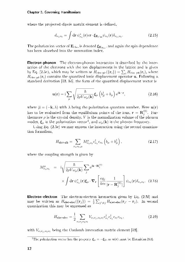
where the projected dipole matrix element is defined,
𝑑𝜈𝑎𝜈𝑏=
∫dr𝜓*
𝜈𝑎(r)𝑒r · 𝜉Eclas
𝜓𝜈𝑏(r)𝛿𝜈𝑎,𝜈𝑏
. (2.15)
The polarization vector of Eclas is denoted 𝜉Eclas, and again the spin dependence
has been absorbed into the summation index.
Electron-phonon The electron-phonon interaction is described by the inter-action of the electrons with the ion displacements in the lattice and is givenby Eq. (2.5e), which may be written as 𝐻elec-ph(r𝑖) =
∑𝑖𝐻elec-ph(r𝑖), where
𝐻elec-ph(r𝑖) contains the quantized ionic displacement operator u. Following astandard derivation [53, 55], the form of the quantized displacement vector is
u(r) = i∑𝜇
√~
2𝜌𝑉 𝜔𝜇(k)𝜉𝜇
(𝑏†𝜇 + 𝑏𝜇
)eik · r, (2.16)
where 𝜇 = (−k, 𝜆) with 𝜆 being the polarization quantum number. Here u(r)
has to be evaluated from the equilibrium points of the ions, r = R(0)𝑗 . Fur-
thermore 𝜌 is the crystal density, 𝑉 is the normalization volume of the phononmodes, 𝜉𝜇 is the polarization vector4, and 𝜔𝜇(k) is the phonon frequency.
Using Eq. (2.5e) we may express the interaction using the second quantiza-tion formalism,
𝐻elec-ph =∑
𝜈𝑎𝜈𝑏,𝜇
𝑀𝜇𝜈𝑎𝜈𝑏
𝑐†𝜈𝑎𝑐𝜈𝑏
(𝑏𝜇 + 𝑏†
), (2.17)
where the coupling strength is given by
𝑀𝜇𝜈𝑎𝜈𝑏
= i
√~
2𝜌𝑉 𝜔𝜇(k)
∑𝑗
eik ·R(0)𝑗
×∫
dr𝜓*𝜈𝑎
(r)𝜉𝜇 ·∇r
[𝑒𝑞𝑗4𝜋𝜖
1
|r−R(0)𝑗 |
]𝜓𝜈𝑏
(r)𝛿𝜈𝑎𝜈𝑏. (2.18)
Electron-electron The electron-electron interaction given by Eq. (2.5f) andmay be written as 𝐻elec-elec(r𝑗) = 1
2
∑𝑗′ =𝑗 𝐻elec-elec(r𝑗′ − r𝑗). In second
quantization this may be expressed as
𝐻elec-elec =1
2
∑𝜈𝑖𝜈𝑗𝜈𝑘𝜈𝑙
𝑉𝜈𝑖𝜈𝑗 ,𝜈𝑘𝜈𝑙𝑐†𝜈𝑖𝑐†𝜈𝑗𝑐𝜈𝑙𝑐𝜈𝑘
, (2.19)
with 𝑉𝜈𝑖𝜈𝑗 ,𝜈𝑘𝜈𝑙being the Coulomb intercation matrix element [53].
4The polarization vector has the property 𝜉𝜇 = −𝜉𝜇, as u(r) must be Hermitian [53].
12
Many-body Hamiltonian
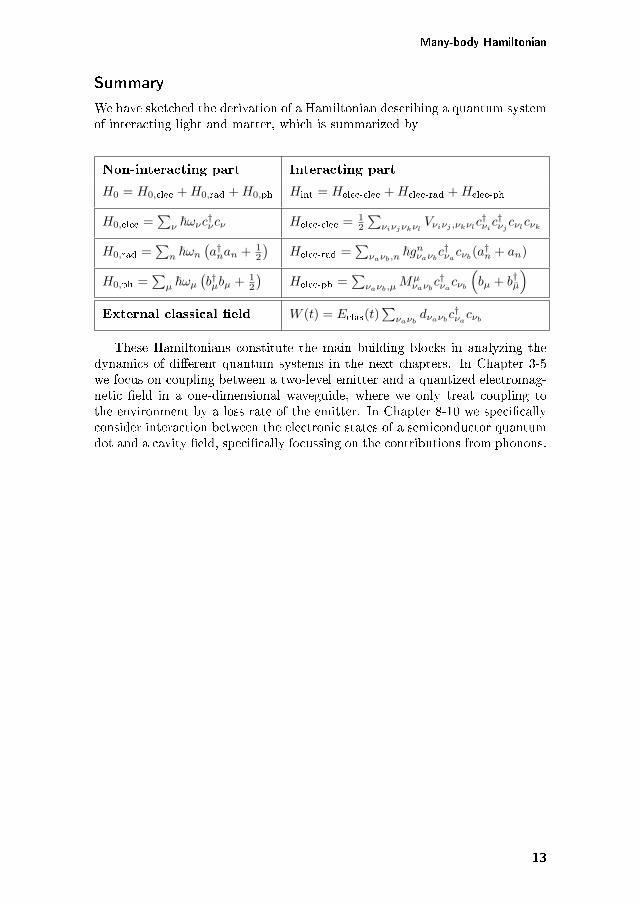
Summary
We have sketched the derivation of a Hamiltonian describing a quantum systemof interacting light and matter, which is summarized by
Non-interacting part Interacting part
𝐻0 = 𝐻0,elec +𝐻0,rad +𝐻0,ph 𝐻int = 𝐻elec-elec +𝐻elec-rad +𝐻elec-ph
𝐻0,elec =∑
𝜈 ~𝜔𝜈𝑐†𝜈𝑐𝜈 𝐻elec-elec = 1
2
∑𝜈𝑖𝜈𝑗𝜈𝑘𝜈𝑙
𝑉𝜈𝑖𝜈𝑗 ,𝜈𝑘𝜈𝑙𝑐†𝜈𝑖𝑐†𝜈𝑗𝑐𝜈𝑙𝑐𝜈𝑘
𝐻0,rad =∑
𝑛 ~𝜔𝑛
(𝑎†𝑛𝑎𝑛 + 1
2
)𝐻elec-rad =
∑𝜈𝑎𝜈𝑏,𝑛
~𝑔𝑛𝜈𝑎𝜈𝑏𝑐†𝜈𝑎
𝑐𝜈𝑏(𝑎†𝑛 + 𝑎𝑛)
𝐻0,ph =∑
𝜇 ~𝜔𝜇
(𝑏†𝜇𝑏𝜇 + 1
2
)𝐻elec-ph =
∑𝜈𝑎𝜈𝑏,𝜇
𝑀𝜇𝜈𝑎𝜈𝑏
𝑐†𝜈𝑎𝑐𝜈𝑏
(𝑏𝜇 + 𝑏†
)External classical field 𝑊 (𝑡) = 𝐸clas(𝑡)
∑𝜈𝑎𝜈𝑏
𝑑𝜈𝑎𝜈𝑏𝑐†𝜈𝑎
𝑐𝜈𝑏
These Hamiltonians constitute the main building blocks in analyzing thedynamics of different quantum systems in the next chapters. In Chapter 3-5we focus on coupling between a two-level emitter and a quantized electromag-netic field in a one-dimensional waveguide, where we only treat coupling tothe environment by a loss rate of the emitter. In Chapter 8-10 we specificallyconsider interaction between the electronic states of a semiconductor quantumdot and a cavity field, specifically focussing on the contributions from phonons.
13

Chapter 3
Single-photon scattering
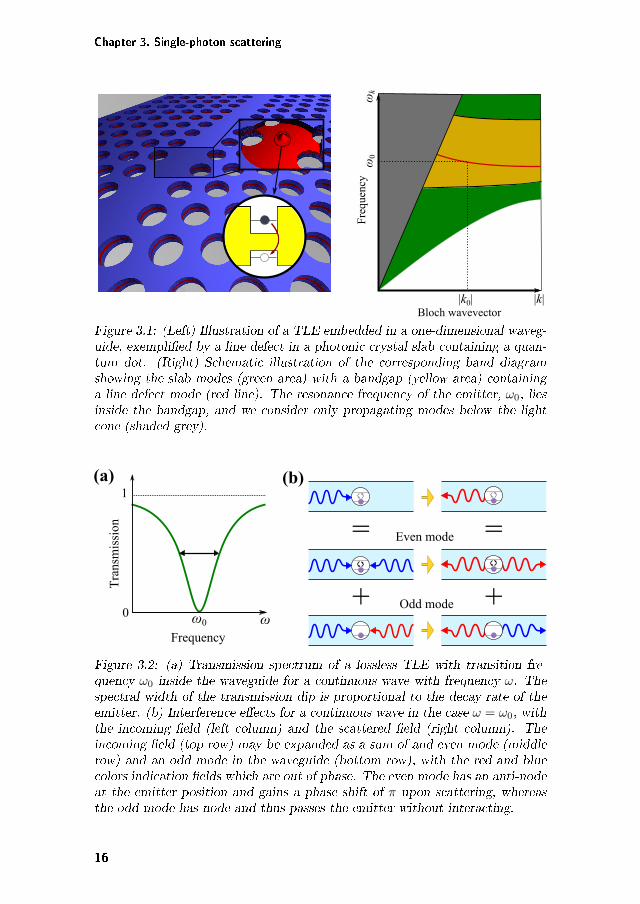
One of the simplest systems in which to investigate the coupling between afew-photon non-linearity and a propagating photon pulse, is a two-level emit-ter (TLE) coupling to an infinite one-dimensional waveguide. A physical re-alization of such a system has e.g. been demonstrated by A. Goban et al.[62] by trapping a Caesium atom in the vicinity of a photonic crystal waveg-uide, demonstrating a coupling efficieny of the TLE to the waveguide modesof 32 %. A much higher coupling efficiency may, however, be achieved in solidstate systems, in which the TLE is placed inside the high-index materials. Arecent experiment by M. Arcari et al. [45] demonstrates a coupling efficiencyof 98 % between a semiconductor quantum dot and a line defect in a photoniccrystal slab, as sketched in Fig. 3.1. A higher coupling for the quantum dot isachieved as the emitter is inside the high-index material, although the solid en-vironment also introduce additional scattering processes from phonons, whichwe will elaborate on in Chapter 8–10. The purpose of this chapter is to clarifythe dynamics of a single photon scattering on the TLE, as it is an importantbuilding block for a solid understanding of two-photon scattering, where thenon-linearity of the TLE is addressed.
The scattering of an incoming single-photon wavepacket on the TLE willdepend strongly on the spectral and spatial properties of the photon relative tothe TLE. Pulses with a very narrow bandwidth have a very small probabilityof exciting the TLE, as the energy of the pulse is spread across a wide spatialrange. In this regime, the TLE is well-known to behave as a linear scatterer inthe few-photon limit with the transmission spectrum sketched in Fig. 3.2(a). Ifthe narrow-spectrum photon is resonant with the emitter transition, the pulseis fully reflected. The reason for this is explained in Fig. 3.2(b), by expanding aright-propagating photon in an equal superposition of even and odd waveguidemodes. While the even modes has an anti-node at the emitter position, theodd modes has a node and thus does not interact with the emitter. As the fieldscattered from a dipole will be out of phase with the incoming light, the evenmode attains a phase shift of 𝜋, whereas the odd modes propagates past theemitter. Thus, by summing up the contributions, the scattered even and oddmode interfere destructively in the right (transmitted) port, and thus the
15
Chapter 3. Single-photon scattering
|k|
ωk
ω0
|k0|Bloch wavevector
Fre
quen
cy
Figure 3.1: (Left) Illustration of a TLE embedded in a one-dimensional waveg-uide, exemplified by a line defect in a photonic crystal slab containing a quan-tum dot. (Right) Schematic illustration of the corresponding band diagramshowing the slab modes (green area) with a bandgap (yellow area) containinga line defect mode (red line). The resonance frequency of the emitter, 𝜔0, liesinside the bandgap, and we consider only propagating modes below the lightcone (shaded grey).
ωω0
Tra
nsm
issi
on
0
1
Frequency
(a)
Even mode
Odd mode +
=
+
=
(b)
Figure 3.2: (a) Transmission spectrum of a lossless TLE with transition fre-quency 𝜔0 inside the waveguide for a continuous wave with frequency 𝜔. Thespectral width of the transmission dip is proportional to the decay rate of theemitter. (b) Interference effects for a continuous wave in the case 𝜔 = 𝜔0, withthe incoming field (left column) and the scattered field (right column). Theincoming field (top row) may be expanded as a sum of and even mode (middlerow) and an odd mode in the waveguide (bottom row), with the red and bluecolors indication fields which are out of phase. The even mode has an anti-nodeat the emitter position and gains a phase shift of 𝜋 upon scattering, whereasthe odd mode has node and thus passes the emitter without interacting.
16
The model
resonant photon pulse is fully reflected. If the emitter has a non-zero loss rateto other modes than the waveguide modes, the reflection is no longer perfectly100 % [63].
For single-photon pulses with spectral linewidths comparable to that ofthe TLE, the TLE still behaves linearly, as the saturation of the TLE firstplays a role if a second photon is present. Following different approaches todescribe the single-photon scattering [64, 65, 66, 67], we calculate the excitationdynamics of the TLE for input single-photon pulses with different spectra, andwe determine the resulting scattering probabilities. We demonstrate how theincoming pulse is mostly affected by the emitter when the pulse spectrum is asnarrow as possible for resonant excitation, as this would reflect the pulse fully.The emitter, however, is populated the most when the bandwidth of the pulseand the emitter linewidth are comparable, making this regime interesting forinvestigating the emitter non-linearity.
Lastly, we introduce a numerical scheme for solving the single-photon scat-tering for arbitrary pulses, which Chapter 4 will be generalized to two-photonscattering. A full understanding of the mathematical approaches and resultsin the single-photon case is thus important when expanding the model to con-sidering two-photon scattering, as will be done in the next chapters.
3.1 The model
The system Hamiltonian in the Schrödinger picture for a single TLE interactingwith a quantized electromagnetic field is given by Eqs. (2.6), (2.8), and (2.12),neglecting the contribution to the energy from the vacuum field, as this doesnot affect the system dynamics,
𝐻 = ~𝜔0𝑐†𝑐+
∑𝜆
~𝜔𝜆𝑎†𝜆𝑎𝜆 + ~
∑𝜆
[𝑔𝜆𝑎𝜆𝑐† + 𝑔*𝜆𝑎
†𝜆𝑐]. (3.1)
Here 𝜆 is a generalised quantum number describing polarisation and propaga-tion degrees of freedom, and each mode is described by creation and annihila-tion operators 𝑎†𝜆 and 𝑎𝜆, respectively. Furthermore 𝑐† = 𝑐†𝑒𝑐𝑔 is the creationoperator for an excitation of the TLE, moving an electron from the ground stateto the excitated state. The transmission frequency of the emitter is denoted𝜔0, and the coupling between the TLE and the optical mode 𝜆 is describedby the dipole interaction by the strength 𝑔𝜆 from in Eq. (2.13). In Eq. (3.1)the rapidly-oscillation interaction terms containing 𝑎†𝜆𝑐
† and 𝑎𝜆𝑐 have been ne-glected by the rotating wave approximation, valid when the electromagneticfield has frequencies close to the emitter resonance, with low field intensities[68].
We assume that the waveguide is sufficiently small, such that it only sup-ports a single mode (for each direction of propagation) at a specific frequency, assketched for the photonic crystal waveguide in Fig. 3.1. In this case, the modeindex 𝜆 corresponds to the continuous-mode variable 𝑘, being the wavenumberof the plane wave modes. Here 𝑘 > 0 or 𝑘 < 0 implies a waveguide modepropagating in the forward or backward direction, respectively. For the infinitewaveguide, these modes will be plane wave modes.
17
Chapter 3. Single-photon scattering
With these assumptions, the sum over all modes in the waveguide reducesto∑
𝜆 = lim𝐿→∞(𝐿/2𝜋)∫∞−∞ d𝑘 , with 𝐿 being the length of the 1D waveguide,
and 2𝜋/𝐿 the spacing between the modes in reciprocal space. Continuous modeoperators are defined as 𝑎(𝑘) = lim𝐿→∞
√(𝐿/2𝜋)𝑎𝜆, preserving the commu-
tator relationship [𝑎(𝑘), 𝑎†(𝑘′)] = 𝛿(𝑘 − 𝑘′) [69, 50]. Moreover, the continuousversion of the waveguide mode frequencies and coupling strength is defined as𝜔(𝑘) = 𝜔𝜆 and 𝑔(𝑘) = lim𝐿→∞
√(𝐿/2𝜋)𝑔𝜆, respectively. The system Hamil-
tonian becomes
𝐻 = ~𝜔0𝑐†𝑐+
∫ ∞
−∞d𝑘 ~𝜔(𝑘)𝑎(𝑘)†𝑎(𝑘) + ~
∫ ∞
−∞d𝑘[𝑔(𝑘)𝑎(𝑘)𝑐† + h.c.
], (3.2)
with h.c. indicating a term which is the Hermitian conjugate of the previousterm.
The calculations are most easily carried out in a frame rotating with acarrier frequency of the emitter, 𝜔0, described by the transformation 𝑇 (𝑡) =
exp[−i𝜔0𝑡(𝑐†𝑐 +
∑𝜆 𝑎
†𝜆𝑎𝜆)]. The transformed Hamiltonian is given by =
𝑇 †(𝑡)𝐻𝑇 (𝑡) + i~𝜕𝑇 †
𝜕𝑡 𝑇 (𝑡) = 0 +𝐻𝐼 , resulting in
=
∫ ∞
−∞d𝑘 ~(𝜔(𝑘) − 𝜔0)𝑎(𝑘)†𝑎(𝑘) + ~
∫ ∞
−∞d𝑘[𝑔(𝑘)𝑎(𝑘)𝑐† + h.c.
]. (3.3)
The incoming photon wavepackets are assumed to have a small bandwidth (onthe order of 109 rad s−1) compared to the QD transition frequency (∼ 1015 rads−1). This allows a linearization of the dispersion relation (for each directionof propagation), obtained by a Taylor expansion of the dispersion relation 𝜔(𝑘)around 𝜔0, see Fig. 3.1,
𝜔(𝑘) − 𝜔0 =𝜕𝜔
𝜕𝑘
𝑘=±𝑘0
(𝑘 ∓ 𝑘0) = 𝑣𝑔(|𝑘| − 𝑘0), (3.4)
valid for photons propagating in both directions, with 𝑘0 > 0 defined such that𝜔(𝑘0) = 𝜔0, and with the group velocity 𝑣𝑔 = 𝜕𝜔
𝜕𝑘 |𝑘=𝑘0.
3.2 A single system excitation
We consider a single excitation in the emitter-waveguide system, assuming nolosses of the excitation to external reservoirs1, which would be a reasonableapproximation for the QD–photonic crystal waveguide coupling demonstratedin Ref. [45]. The system state may at all times be written as a superposition ofthe excitation being in one of the waveguide modes or as an electronic excitationin the emitter,
|𝜓(𝑡)⟩ =
∫ ∞
−∞d𝑘 𝐶𝑔(𝑘, 𝑡)𝑎†(𝑘)|𝜑⟩ + 𝐶𝑒(𝑡)𝑐†|𝜑⟩, (3.5)
1For non-negligible loss, e.g. due to the presence of other modes or due to scattering withphonons, external reservoirs to which the system couples may be introduced. In the limit ofweak coupling to a reservoir of harmonic oscillators, dissipation rates of the system statesmay be derived [70]. Alternatively, the dynamics may be treated using a quantum jumpapproach [71] or reduced density matrices [72, 73], which however are computationally morechallenging.
18
A single system excitation
with |𝜑⟩ being the quantum state with the emitter in its ground state and nophotons in the waveguide. The wavefunction is normalized such that ⟨𝜓(𝑡)|𝜓(𝑡)⟩ =∫∞−∞ d𝑘 |𝐶𝑔(𝑘, 𝑡)|2 + |𝐶𝑒(𝑡)|2 = 1 at all times, in the loss-free case.The system dynamics are calculated by applying the time-dependent Schrödinger
equation, i~𝜕𝑡|𝜓(𝑡)⟩ = 𝐻|𝜓(𝑡)⟩, and projecting onto the orthogonal states 𝑐†|𝜑⟩and 𝑎†(𝑘′)|𝜑⟩, giving a system of coupled differential equations for the expan-sion coefficients,
𝜕𝑡𝐶𝑒(𝑡) = −i
∫ ∞
−∞d𝑘 𝑔(𝑘)𝐶𝑔(𝑘, 𝑡), (3.6a)
𝜕𝑡𝐶𝑔(𝑘, 𝑡) = −i[𝜔(𝑘) − 𝜔0]𝐶𝑔(𝑘, 𝑡) − i𝑔*(𝑘)𝐶𝑒(𝑡). (3.6b)
By formally integrating Eq. (3.6b) from an initial time 𝑡𝑖 to 𝑡, and insertingthe expression for 𝐶𝑔(𝑘, 𝑡) back into Eq. (3.6a), we obtain
𝜕𝑡𝐶𝑒(𝑡) = −i
∫ ∞
−∞d𝑘 𝑔(𝑘)𝐶𝑔(𝑘, 𝑡𝑖)e
−i[𝜔(𝑘)−𝜔0](𝑡−𝑡𝑖)
−∫ ∞
−∞d𝑘 |𝑔(𝑘)|2
∫ 𝑡
𝑡𝑖
d𝑡′ 𝐶𝑒(𝑡′)e−i[𝜔(𝑘)−𝜔0](𝑡−𝑡′). (3.7)
The intergrand in the last term of Eq. (3.7) may be simplified by using theassumption from the previous section that the decay rate of the emitter is muchlower than the carrier frequency of the pulse. In that case, 𝐶𝑒(𝑡′) varies slowlycompared to the exponential and may be pulled outside the integral, as theintegral only has non-zero contributions for 𝑡′ ≈ 𝑡. By this, the lower limit ofthe integration may also be expanded to 𝑡𝑖 → −∞ without changing the valueof the integral. This is well-known as the Wigner-Weisskopf approximation [74],by which the system does not have any memory of the past (also sometimescalled the Markov approximation).
By complex integration, the remaining integral reduces to∫ 𝑡
−∞d𝑡′ e−i[𝜔(𝑘)−𝜔0](𝑡−𝑡′) = −i𝒫
1
𝜔(𝑘) − 𝜔0
+ 𝜋𝛿(𝜔(𝑘) − 𝜔0), (3.8)
with 𝒫 indicating the principal value. The first term induces a frequency shift,commonly known as the Lamb shift [50], which is omitted by including thisas a re-normalization of the basic transition frequency of the emitter, 𝜔0. Bydefining the constant Γ = 2𝜋
∫ −∞−∞ d𝑘 |𝑔(𝑘)|2𝛿(𝜔(𝑘) − 𝜔0), we arrive at
𝜕𝑡𝐶𝑒(𝑡) = −i
∫ ∞
−∞d𝑘 𝑔(𝑘)𝐶𝑔(𝑘, 𝑡𝑖)e
−i[𝜔(𝑘)−𝜔0](𝑡−𝑡𝑖) − Γ
2𝐶𝑒(𝑡). (3.9)
Hence, Γ is spontaneous decay rate of the emitter population, |𝐶𝑒(𝑡)|2, intoboth propagation directions of the waveguide. Under the narrow bandwidthassumptions, 𝑔(𝑘) is approximately contrant, 𝑔(𝑘) ≈ 𝑔(𝑘𝑝) =
√Γ𝑣𝑔/(4𝜋) [43].
3.2.1 Input state
To solve Eq. (3.9) we consider a incident, forward-propagating single photonas the initial condition. A single-photon state existing in a 1D continuum is in
19
Chapter 3. Single-photon scattering
−4 −2 0 2 40
0.5
1
z-Z0 [units of vg/Γ]
Inte
nsit
y
−2 −1 0 1 2
LorentzGaussSquare
k-k0 [units of Γ/vg]
0
0.5
1
Inte
nsit
y
(a) (b)
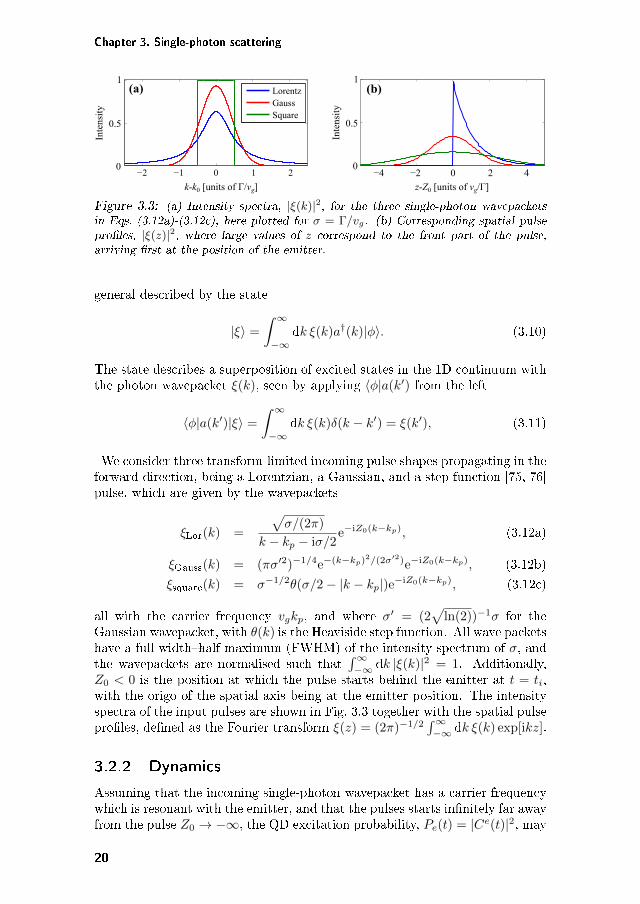
Figure 3.3: (a) Intensity spectra, |𝜉(𝑘)|2, for the three single-photon wavepacketsin Eqs. (3.12a)-(3.12c), here plotted for 𝜎 = Γ/𝑣𝑔. (b) Corresponding spatial pulseprofiles, |𝜉(𝑧)|2, where large values of 𝑧 correspond to the front part of the pulse,arriving first at the position of the emitter.
general described by the state
|𝜉⟩ =
∫ ∞
−∞d𝑘 𝜉(𝑘)𝑎†(𝑘)|𝜑⟩. (3.10)
The state describes a superposition of excited states in the 1D continuum withthe photon wavepacket 𝜉(𝑘), seen by applying ⟨𝜑|𝑎(𝑘′) from the left
⟨𝜑|𝑎(𝑘′)|𝜉⟩ =
∫ ∞
−∞d𝑘 𝜉(𝑘)𝛿(𝑘 − 𝑘′) = 𝜉(𝑘′), (3.11)
We consider three transform-limited incoming pulse shapes propagating in theforward direction, being a Lorentzian, a Gaussian, and a step-function [75, 76]pulse, which are given by the wavepackets
𝜉Lor(𝑘) =
√𝜎/(2𝜋)
𝑘 − 𝑘𝑝 − i𝜎/2e−i𝑍0(𝑘−𝑘𝑝), (3.12a)
𝜉Gauss(𝑘) = (𝜋𝜎′2)−1/4e−(𝑘−𝑘𝑝)2/(2𝜎′2)e−i𝑍0(𝑘−𝑘𝑝), (3.12b)
𝜉square(𝑘) = 𝜎−1/2𝜃(𝜎/2 − |𝑘 − 𝑘𝑝|)e−i𝑍0(𝑘−𝑘𝑝), (3.12c)
all with the carrier frequency 𝑣𝑔𝑘𝑝, and where 𝜎′ = (2√
ln(2))−1𝜎 for theGaussian wavepacket, with 𝜃(𝑘) is the Heaviside step function. All wave packetshave a full width–half maximum (FWHM) of the intensity spectrum of 𝜎, andthe wavepackets are normalised such that
∫∞−∞ d𝑘 |𝜉(𝑘)|2 = 1. Additionally,
𝑍0 < 0 is the position at which the pulse starts behind the emitter at 𝑡 = 𝑡𝑖,with the origo of the spatial axis being at the emitter position. The intensityspectra of the input pulses are shown in Fig. 3.3 together with the spatial pulseprofiles, defined as the Fourier transform 𝜉(𝑧) = (2𝜋)−1/2
∫∞−∞ d𝑘 𝜉(𝑘) exp[i𝑘𝑧].
3.2.2 Dynamics
Assuming that the incoming single-photon wavepacket has a carrier frequencywhich is resonant with the emitter, and that the pulses starts infinitely far awayfrom the pulse 𝑍0 → −∞, the QD excitation probability, 𝑃𝑒(𝑡) = |𝐶𝑒(𝑡)|2, may
20
A single system excitation
Forward[propagatingBackward[propagating
t[=[0
t[=[8/Γ[
t[=[10/Γ[
t[=[15/Γ[
t[=[20/Γ[
z[=[0
z[=[0
z[=[0
z[=[0
z[=[0z[=[Z0
(c)
0
0.1
Em
itte
r[ex
cita
tion
0.2
0.3
0.4
0.5
-4 -2 0 2 4 6
t + Z0/vg[[units[of[1/Γ][
LorentzGaussSquare
(a)
0
0.1
Max
imal
[em
itte
r[ex
cita
tion
0.2
0.3
0.4
0.5
0 0.5 1 1.5 2 2.5 3
σ[[units[of[Γ/vg][
(b)
LorentzGaussSquare
Figure 3.4: (a) Emitter excitation probability for an incoming single-photonwavepacket starting in 𝑧 = 𝑍0 < 0 with 𝜎 = 2Γ/𝑣𝑔, for the wavepackets in Eqs.(3.13a)-(3.13c), resonant with the emitter, 𝑘𝑝 = 𝑘0. (b) Maximal emitter excitationduring the scattering event for incoming pulses with different values of 𝜎, also with𝑘𝑝 = 𝑘0. (c) Excitation density in the waveguide for light propagating in the forward(yellow) and backward (blue) direction for a Gaussian pulse scattering on the emitterat 𝑧 = 0 (red). Figure (c) is reproduced from [77].
be determined by solving Eq. (3.9) with the initial conditions 𝐶𝑔(𝑘, 𝑡𝑖) = 𝜉(𝑘)and 𝐶𝑒(𝑡𝑖) = 0 for the pulse shapes in Eqs. (3.12a)-(3.12c),
𝑃Lor𝑒 (𝑡) =
2Γ𝑣𝑔𝜎
(𝜎𝑣𝑔 + Γ)2
[e𝜎𝑣𝑔𝜏𝜃(−𝜏) + e−Γ𝜏𝜃(𝜏)
], (3.13a)
𝑃Gauss𝑒 (𝑡) =
√𝜋Γ
4𝑣𝑔𝜎′ e−Γ𝜏+Γ2/(4𝜎′2𝑣2
𝑔)
[1 − erf
(Γ − 2𝑣2𝑔𝜎
′2𝜏
2√
2𝜎′𝑣𝑔
)]2, (3.13b)
𝑃 square𝑒 (𝑡) =
Γ
4𝜋𝑣𝑔𝜎e−Γ𝜏
𝐸1
(i𝜎𝑣𝑔 − Γ
2𝜏
)− 𝐸1
(−i𝜎𝑣𝑔 − Γ
2𝜏
) 2, (3.13c)
with 𝜏 = 𝑡+𝑍0/𝑣𝑔 being the time in a frame relative to the initial position ofthe pulse. Additionally, the error function is defined as erf(𝑥) = 2√
𝜋
∫ 𝑥
0d𝑞 e−𝑞2 ,
and 𝐸1 is the exponential integral defined as 𝐸1(𝑧) =∫∞1
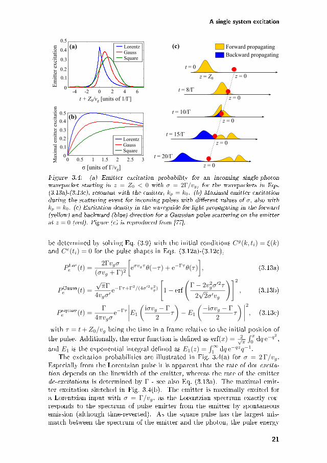
d𝑞 e−𝑞𝑧𝑞−1.The excitation probabilities are illustrated in Fig. 3.4(a) for 𝜎 = 2 Γ/𝑣𝑔.
Especially from the Lorentzian pulse it is apparent that the rate of dot excita-tion depends on the linewidth of the emitter, whereas the rate of the emitterde-excitations is determined by Γ - see also Eq. (3.13a). The maximal emit-ter excitation sketched in Fig. 3.4(b). The emitter is maximally excited fora Lorentzian input with 𝜎 = Γ/𝑣𝑔, as the Lorentzian spectrum exactly cor-responds to the spectrum of pulse emitter from the emitter by spontaneousemission (although time-reverted). As the square pulse has the largest mis-match between the spectrum of the emitter and the photon, the pulse energy
21
Chapter 3. Single-photon scattering
can never efficiently couple to the emitter and thus results in the lowest maxi-mal emission probability for the square pulse. The maximal attainable emitterpopulation of 1/2 stems from the phenomenon in Fig. 3.2, as only maximallyhalf of the photon energy may couple to the emitter.
The properties of the scattered pulse may be examined by calculating theenergy distribution across the waveguide at a time 𝑡 during the scattering event.We describe it by the waveguide excitation density, 𝑁𝑧(𝑧, 𝑡), measured in unitsof of inverse length. It is calculated using Eq. (3.6b), and is defined as
𝑁𝑧(𝑧, 𝑡) = ⟨𝜓(𝑡)|𝑎(𝑧)𝑎†(𝑧)|𝜓(𝑡)⟩ (3.14)
=1
2𝜋
∫ ∞
−∞d𝑘 𝐶𝑔(𝑘, 𝑡)ei𝑘𝑧
2. (3.15)
The excitation density is sketched in Fig. 3.4(c) for scattering of a Gaussianpulse. Due to the finite spatial width of the pulse (and thus non-zero band-width), there is a probability that the pulse scatters in both directions, andmoreover the spatial pulse profile may be significantly changed by the scatter-ing.
The scattered state may be obtained by calculating 𝐶𝑔(𝑘, 𝑡) for 𝑡 → ∞.An easier way to obtain the scattered state is, however, by exploiting thatthe emitter acts as linear scatterer for a single-photon packet, and thus thescattered wavepacket may be calculated by treating each frequency componentof the incoming pulse individually. For an input pulse as in Eq. (3.10) whichpropagates in the forward direction, the wavepacket of the scattered state is
𝜉scat(𝑝) =
∫ ∞
−∞d𝑘 𝜉(𝑘) [𝑡(𝑘)𝛿(𝑝− 𝑘) + 𝑟(𝑘)𝛿(𝑝+ 𝑘)]
= 𝜉(𝑝)𝑡(𝑝) + 𝜉(−𝑝)𝑟(−𝑝), (3.16)
where the transmission and reflection coefficients for scattering on the emitteris [66],
𝑡(𝑘) =𝑘 − 𝑘0
𝑘 − 𝑘0 + iΓ/2, 𝑟(𝑘) =
−iΓ/2
𝑘 − 𝑘0 + iΓ/2, (3.17)
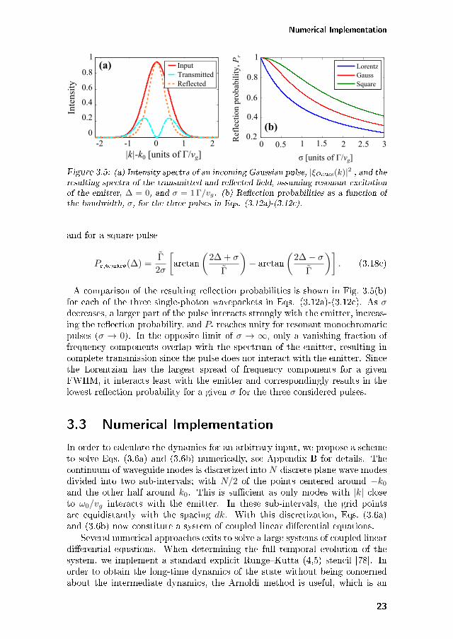
with Γ = Γ/𝑣𝑔. The spectrum for the transmitted part, |𝜉(𝑝)𝑡(𝑝)|2, and for thereflected part, |𝜉(−𝑝)𝑟(−𝑝)|2, is shown in Fig. 3.5(a). The frequency compo-nents of the pulse closest to the transition energy of the emitter interact moststrongly, and those at the exact frequency of the emitter (𝑘 = 𝑘0) are perfectlyreflected [64]. The probability the photon is scattered is obtained by integrat-ing over all pulse frequencies, 𝑃r =
∫∞−∞ d𝑝 |𝜉(−𝑝)𝑟(−𝑝)|2. For a Lorentzian
input, the reflection probability becomes
𝑃r,Lor(∆) =(Γ + 𝜎)Γ
(Γ + 𝜎)2 + 4∆2, (3.18a)
with the detuning between the emitter and the pulse defined as ∆ = 𝑘𝑝 − 𝑘0.For a resonant Gaussian pulse, ∆ = 0,
𝑃r,Gauss(∆ = 0) =Γ√𝜋
2𝜎′ eΓ2/(2𝜎′)2
[1 − erf
(Γ
2𝜎′
)], (3.18b)
22
Numerical Implementation
0.2
0.4
0.6
0.8
1(a) Lorentz
GaussSquare
Ref
lect
ion3
prob
abil
ity,
3Pr
0 0.5 1 1.5 2 2.5 3
σ3[units3of3Γ/vg]3
(b)
InputTransmittedReflected
Inte
nsit
y 0.6
0
0.2
0.8
0.4
-2 -1 0 1 2|k|-k03[units3of3Γ/vg]3
1
Figure 3.5: (a) Intensity spectra of an incoming Gaussian pulse, |𝜉Gauss(𝑘)|2 , and theresulting spectra of the transmitted and reflected field, assuming resonant excitationof the emitter, Δ = 0, and 𝜎 = 1Γ/𝑣𝑔. (b) Reflection probabilities as a function ofthe bandwidth, 𝜎, for the three pulses in Eqs. (3.12a)-(3.12c).
and for a square pulse
𝑃r,square(∆) =Γ
2𝜎
[arctan
(2∆ + 𝜎
Γ
)− arctan
(2∆ − 𝜎
Γ
)]. (3.18c)
A comparison of the resulting reflection probabilities is shown in Fig. 3.5(b)for each of the three single-photon wavepackets in Eqs. (3.12a)-(3.12c). As 𝜎decreases, a larger part of the pulse interacts strongly with the emitter, increas-ing the reflection probability, and 𝑃r reaches unity for resonant monochromaticpulses (𝜎 → 0). In the opposite limit of 𝜎 → ∞, only a vanishing fraction offrequency components overlap with the spectrum of the emitter, resulting incomplete transmission since the pulse does not interact with the emitter. Sincethe Lorentzian has the largest spread of frequency components for a givenFWHM, it interacts least with the emitter and correspondingly results in thelowest reflection probability for a given 𝜎 for the three considered pulses.
3.3 Numerical Implementation
In order to calculate the dynamics for an arbitrary input, we propose a schemeto solve Eqs. (3.6a) and (3.6b) numerically, see Appendix B for details. Thecontinuum of waveguide modes is discretized into 𝑁 discrete plane wave modesdivided into two sub-intervals; with 𝑁/2 of the points centered around −𝑘0and the other half around 𝑘0. This is sufficient as only modes with |𝑘| closeto 𝜔0/𝑣𝑔 interacts with the emitter. In these sub-intervals, the grid pointsare equidistantly with the spacing 𝑑𝑘. With this discretization, Eqs. (3.6a)and (3.6b) now constitute a system of coupled linear differential equations.
Several numerical approaches exits to solve a large systems of coupled lineardifferential equations. When determining the full temporal evolution of thesystem, we implement a standard explicit Runge–Kutta (4,5) stencil [78]. Inorder to obtain the long-time dynamics of the state without being concernedabout the intermediate dynamics, the Arnoldi method is useful, which is an
23
Chapter 3. Single-photon scattering
−2 0 20
0.5
1
0 10 20 300
0.2
0.4
0
0.5
1
300
0.2
0.4
−5 0 50
0.5
1
0 10 20 300
0.2
0.4
−2 0 2
0 10 20
Analy.Num.
|ξ(k
)|2P
e(t)
t6[units6of61/Γ] t6[units6of61/Γ] t6[units6of61/Γ]
k6[units6of6Γ/vg] k6[units6of6Γ/vg] k6[units6of6Γ/vg]
N6=630,6dk6=60.50 N6=660,6dk6=60.25 N6=6120,6dk6=60.25
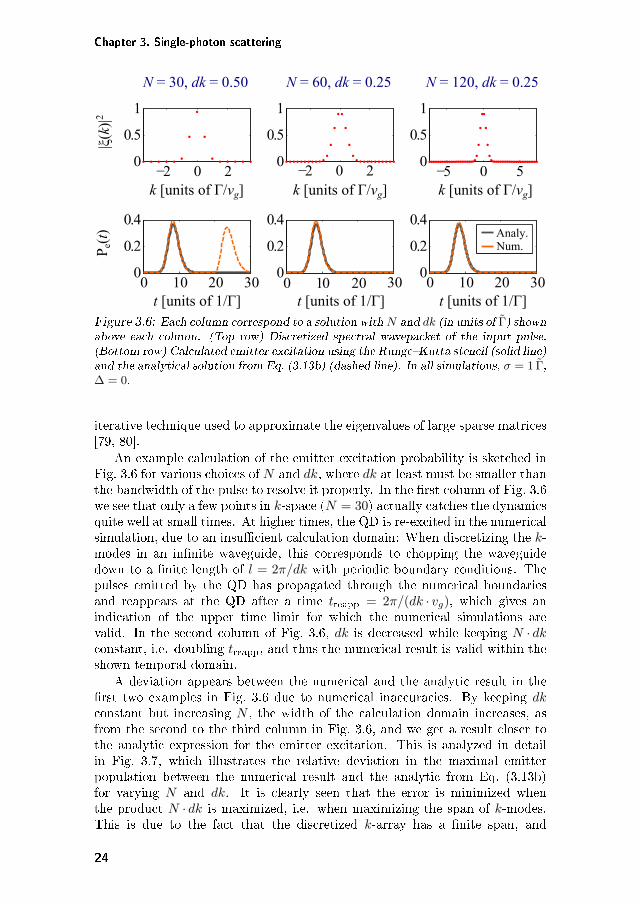
Figure 3.6: Each column correspond to a solution with𝑁 and 𝑑𝑘 (in units of Γ) shownabove each column. (Top row) Discretized spectral wavepacket of the input pulse.(Bottom row) Calculated emitter excitation using the Runge–Kutta stencil (solid line)and the analytical solution from Eq. (3.13b) (dashed line). In all simulations, 𝜎 = 1 Γ,Δ = 0.
iterative technique used to approximate the eigenvalues of large sparse matrices[79, 80].
An example calculation of the emitter excitation probability is sketched inFig. 3.6 for various choices of 𝑁 and 𝑑𝑘, where 𝑑𝑘 at least must be smaller thanthe bandwidth of the pulse to resolve it properly. In the first column of Fig. 3.6we see that only a few points in 𝑘-space (𝑁 = 30) actually catches the dynamicsquite well at small times. At higher times, the QD is re-excited in the numericalsimulation, due to an insufficient calculation domain: When discretizing the 𝑘-modes in an infinite waveguide, this corresponds to chopping the waveguidedown to a finite length of 𝑙 = 2𝜋/𝑑𝑘 with periodic boundary conditions. Thepulses emitted by the QD has propagated through the numerical boundariesand reappears at the QD after a time 𝑡reapp = 2𝜋/(𝑑𝑘 · 𝑣𝑔), which gives anindication of the upper time limit for which the numerical simulations arevalid. In the second column of Fig. 3.6, 𝑑𝑘 is decreased while keeping 𝑁 · 𝑑𝑘constant, i.e. doubling 𝑡reapp, and thus the numerical result is valid within theshown temporal domain.
A deviation appears between the numerical and the analytic result in thefirst two examples in Fig. 3.6 due to numerical inaccuracies. By keeping 𝑑𝑘constant but increasing 𝑁 , the width of the calculation domain increases, asfrom the second to the third column in Fig. 3.6, and we get a result closer tothe analytic expression for the emitter excitation. This is analyzed in detailin Fig. 3.7, which illustrates the relative deviation in the maximal emitterpopulation between the numerical result and the analytic from Eq. (3.13b)for varying 𝑁 and 𝑑𝑘. It is clearly seen that the error is minimized whenthe product 𝑁 · 𝑑𝑘 is maximized, i.e. when maximizing the span of 𝑘-modes.This is due to the fact that the discretized 𝑘-array has a finite span, and
24
Summary
0.1
0.01
0.001
0.1
0.2
0.3
0.4
0.5100 200 300 400 500 600
dk
[uni
ts o
f Γ
/vg]
N
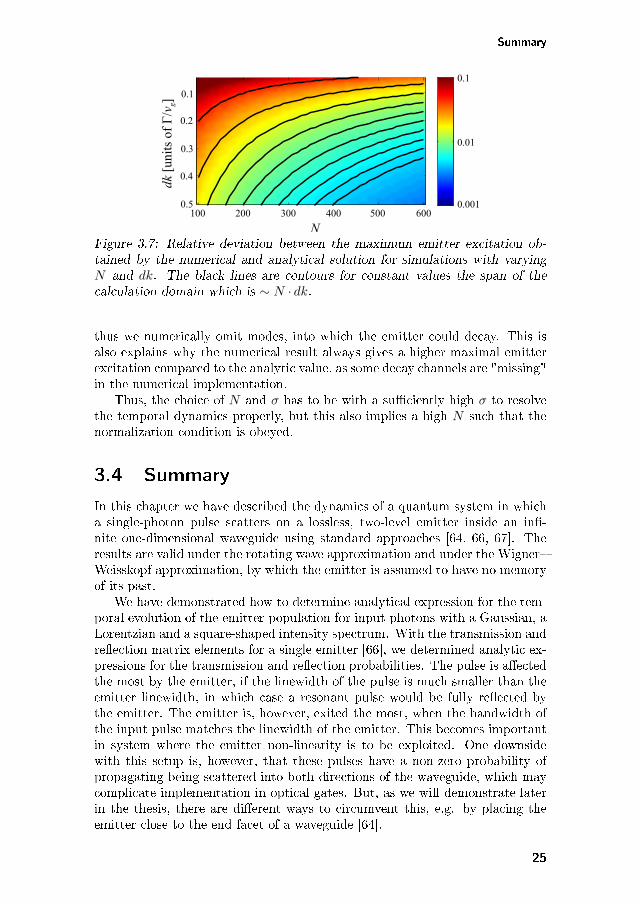
Figure 3.7: Relative deviation between the maximum emitter excitation ob-tained by the numerical and analytical solution for simulations with varying𝑁 and 𝑑𝑘. The black lines are contours for constant values the span of thecalculation domain which is ∼ 𝑁 · 𝑑𝑘.
thus we numerically omit modes, into which the emitter could decay. This isalso explains why the numerical result always gives a higher maximal emitterexcitation compared to the analytic value, as some decay channels are "missing"in the numerical implementation.
Thus, the choice of 𝑁 and 𝜎 has to be with a sufficiently high 𝜎 to resolvethe temporal dynamics properly, but this also implies a high 𝑁 such that thenormalization condition is obeyed.
3.4 Summary
In this chapter we have described the dynamics of a quantum system in whicha single-photon pulse scatters on a lossless, two-level emitter inside an infi-nite one-dimensional waveguide using standard approaches [64, 66, 67]. Theresults are valid under the rotating wave approximation and under the Wigner–Weisskopf approximation, by which the emitter is assumed to have no memoryof its past.
We have demonstrated how to determine analytical expression for the tem-poral evolution of the emitter population for input photons with a Gaussian, aLorentzian and a square-shaped intensity spectrum. With the transmission andreflection matrix elements for a single emitter [66], we determined analytic ex-pressions for the transmission and reflection probabilities. The pulse is affectedthe most by the emitter, if the linewidth of the pulse is much smaller than theemitter linewidth, in which case a resonant pulse would be fully reflected bythe emitter. The emitter is, however, exited the most, when the bandwidth ofthe input pulse matches the linewidth of the emitter. This becomes importantin system where the emitter non-linearity is to be exploited. One downsidewith this setup is, however, that these pulses have a non-zero probability ofpropagating being scattered into both directions of the waveguide, which maycomplicate implementation in optical gates. But, as we will demonstrate laterin the thesis, there are different ways to circumvent this, e.g. by placing theemitter close to the end facet of a waveguide [64].
25
Chapter 3. Single-photon scattering
The possibilities with the emitter–waveguide systems are rich, and severalfunctionalities of emitter–waveguide systems have been discussed, such as asingle-photon router by using multiple emitters and waveguides [81]. For emit-ters with more than two energy levels [82], proposals have been made usingthe waveguide–emitter systems as single-photon frequency converters [83] andsingle-photon transistors [43, 84]. Furthermore the approaches demonstratedin this chapter may also be used to analyze more advanced scatterers such aswaveguides interacting with emitters inside optical cavities [85, 86].
With this detailed understanding of the single-photon scattering, we pro-ceed to considering two-photon scatting in the following chapters. Due to thesaturability of the emitter, the two-photon scattering dynamics becomes muchmore complex. In Chapter 4 the scattering is examined using the numericalscheme from Section 3.3, supported by analytical calculations of the emitterexcitation for two uncorrelated, Gaussian pulses, using an approach similarto the approach in Section 3.2. The transmission properties are specificallyconsidered in Chapter 5, using the scattering matrix formalism [66], in whichnon-linear two-photon scattering matrix elements are introduced.
26
Chapter 4
Two-photon scattering —
Wavefunction approach
4.1 Introduction
A model for describing two-photon scattering on a two-level emitter is de-veloped in this chapter, as an extension of the single-excitation results fromChapter 3. The dynamics of two-photon scattering is, however, much morecomplex than the single-photon case, as the non-linear emitter can induce cor-relations between the photons caused by elastic multi-photon scattering pro-cesses [66, 87]. Existing methods for analyzing the multiple-photon scatter-ing problem — such as the input-output formalism [66], the real-space Betheansatz [87, 88], or the Lehmann-Symanzik-Zimmermann formalism [89] — focuson the long-time limit of the scattered state [67] and necessitate the compu-tation of complicated scattering elements or Laplace transforms [90]. Anotherrecent approach demonstrates a master equation formalism derived by startingfrom the Ito Langevin equation, where also the emitter excitation is calcu-lated [72], although without relating the emitter excitation to the scattering-induced correlations. Some specific considerations have been demonstratedusing a wavefunction description of the system [91], e.g. the demonstration ofstimulated emission of an emitter inside a waveguide [92], and scattering of atwo-photon wavepacket in a photonic tight-binding waveguide [93, 94, 95]. Ap-plications which utilize a TLE nonlinearity have been proposed, such as photonsorters and Bell state analyzers [96]. In all these cases the non-linearity of theemitter leads to rich scattering dynamics and scattering-induced correlations.It is the interplay between these highly non-trivial scattering properties andthe excitation dynamics of the emitter which we seek to clarify in this chapter.
To do so we study two-photon scattering on a quantum emitter in a one-dimensional waveguide using a wavefunction approach as introduced in Chap-ter 3, in which the entire system state is explicitly calculated at all timesduring the scattering process, and which therefore provides a detailed pictureof the scattering dynamics. This approach relies on a direct solution of theSchrödinger equation by expanding the complete state in a basis formed by
27
Chapter 4. Two-photon scattering — Wavefunction approach
the TLE and the optical waveguide modes. This allows us to explore varyingwidths and separations of the incoming photons, and provides a convenientand detailed visualization of the temporal dynamics of the scattering process.As a special case, we show that the approach agrees with the above-mentionedmethods in the post-scattering limit, discussed further in Chapter 5. For co-propagating pulses, we find that the transmission properties of the emitterdepend crucially on the pulse width and separation, with closer spaced pulsesgiving rise to a larger proportion of scattered light. For counter-propagatingcoincident pulses we find that the non-linearity of the emitter can give rise tosignificant pulse-dependent directional correlations in the scattered photonicstate. These correlations can be detected by a reduction in coincident clicksin a Hong-Ou-Mandel measurement setup, analogous to a linear beam splitter.Thus, the emitter may act as a non-linear beam-splitter, but only in the regimewhere the spectral width of the photon pulses is similar to the emitter decayrate.
This chapter is structured as follows: In Section 4.2 we introduce the two-excitation model and formalism as an extension of the model in Chapter 3. InSection 4.3 we analyse the scattering dynamics for two co-propagating photonpulses; we examine how the properties of the scattered state depend on theemitter excitation and consider the scattering-induced correlations between thephotons. In Section 4.4 we study scattering of counter-propagating pulses,elucidating the analogy of the quantum emitter and a non-linear beam-splitter.
The chapter is based on the journal publication Scattering of two photonson a quantum emitter in a one-dimensional waveguide: exact dynamics andinduced correlations. New Jour. Phys. 17, 023030 (2015) by A. Nysteen, P. T.Kristensen, D. P. S. McCutcheon, P. Kaer, and J. Mørk.
4.2 Two-excitation model
The model dynamics are described by the Hamiltonian derived in Eq. (3.3) ina frame rotating with the carrier frequency of the emitter,
=
∫ ∞
−∞d𝑘 ~(𝜔(𝑘) − 𝜔0)𝑎(𝑘)†𝑎(𝑘) + ~
∫ ∞
−∞d𝑘[𝑔(𝑘)𝑎(𝑘)𝑐† + h.c.
], (4.1)
where 𝜔(𝑘) is given by the Taylor expansion in Eq. (3.4), with 𝑘 > 0 (𝑘 <0) describing propagating in the forward (backward) direction which in thisexample is the right (left) direction in the waveguide. As discussed in Chapter 3,experimentally high coupling rates between a QD a photonic crystal waveguidemakes it reasonable to omit losses in the calculations [45]. This allows us toexpand a general state of the system in a basis spanned by all the possiblesystem states containing two excitations. The two-excitation basis states are𝑎†(𝑘1)𝑎†(𝑘2)|𝜑⟩ and 𝑎†(𝑘)𝑐†|𝜑⟩, with the former describing two excited planewave modes with wavevectors 𝑘1 and 𝑘2, and the latter describing the stateswhere the emitter is in its excited state and a single waveguide mode with
28
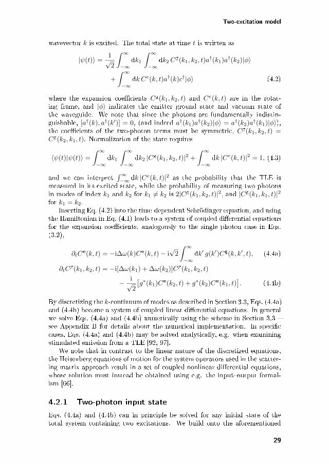
Two-excitation model
wavevector 𝑘 is excited. The total state at time 𝑡 is written as
|𝜓(𝑡)⟩ =1√2
∫ ∞
−∞d𝑘1
∫ ∞
−∞d𝑘2 𝐶
g(𝑘1, 𝑘2, 𝑡)𝑎†(𝑘1)𝑎†(𝑘2)|𝜑⟩
+
∫ ∞
−∞d𝑘 𝐶𝑒(𝑘, 𝑡)𝑎†(𝑘)𝑐†|𝜑⟩ (4.2)
where the expansion coefficients 𝐶g(𝑘1, 𝑘2, 𝑡) and 𝐶𝑒(𝑘, 𝑡) are in the rotat-ing frame, and |𝜑⟩ indicates the emitter ground state and vacuum state ofthe waveguide. We note that since the photons are fundamentally indistin-guishable, [𝑎†(𝑘), 𝑎†(𝑘′)] = 0, (and indeed 𝑎†(𝑘1)𝑎†(𝑘2)|𝜑⟩ = 𝑎†(𝑘2)𝑎†(𝑘1)|𝜑⟩),the coefficients of the two-photon terms must be symmetric, 𝐶g(𝑘1, 𝑘2, 𝑡) =𝐶g(𝑘2, 𝑘1, 𝑡). Normalization of the state requires
⟨𝜓(𝑡)|𝜓(𝑡)⟩ =
∫ ∞
−∞d𝑘1
∫ ∞
−∞d𝑘2 |𝐶g(𝑘1, 𝑘2, 𝑡)|2 +
∫ ∞
−∞d𝑘 |𝐶𝑒(𝑘, 𝑡)|2 = 1, (4.3)
and we can interpret∫∞−∞ d𝑘 |𝐶𝑒(𝑘, 𝑡)|2 as the probability that the TLE is
measured in its excited state, while the probability of measuring two photonsin modes of index 𝑘1 and 𝑘2 for 𝑘1 = 𝑘2 is 2|𝐶g(𝑘1, 𝑘2, 𝑡)|2, and |𝐶g(𝑘1, 𝑘1, 𝑡)|2for 𝑘1 = 𝑘2.
Inserting Eq. (4.2) into the time-dependent Schrödinger equation, and usingthe Hamiltonian in Eq. (4.1) leads to a system of coupled differential equationsfor the expansion coefficients, analogously to the single photon case in Eqs.(3.2),
𝜕𝑡𝐶e(𝑘, 𝑡) = −i∆𝜔(𝑘)𝐶e(𝑘, 𝑡) − i
√2
∫ ∞
−∞d𝑘′ 𝑔(𝑘′)𝐶g(𝑘, 𝑘′, 𝑡), (4.4a)
𝜕𝑡𝐶g(𝑘1, 𝑘2, 𝑡) = −i[∆𝜔(𝑘1) + ∆𝜔(𝑘2)]𝐶g(𝑘1, 𝑘2, 𝑡)
− i√2
[𝑔*(𝑘1)𝐶e(𝑘2, 𝑡) + 𝑔*(𝑘2)𝐶e(𝑘1, 𝑡)
]. (4.4b)
By discretizing the 𝑘-continuum of modes as described in Section 3.3, Eqs. (4.4a)and (4.4b) become a system of coupled linear differential equations. In generalwe solve Eqs. (4.4a) and (4.4b) numerically using the scheme in Section 3.3 –see Appendix B for details about the numerical implementation. In specificcases, Eqs. (4.4a) and (4.4b) may be solved analytically, e.g. when examiningstimulated emission from a TLE [92, 97].
We note that in contrast to the linear nature of the discretized equations,the Heisenberg equations of motion for the system operators used in the scatter-ing matrix approach result in a set of coupled nonlinear differential equations,whose solution must instead be obtained using e.g. the input–output formal-ism [66].
4.2.1 Two-photon input state
Eqs. (4.4a) and (4.4b) can in principle be solved for any initial state of thetotal system containing two excitations. We build onto the aforementioned
29
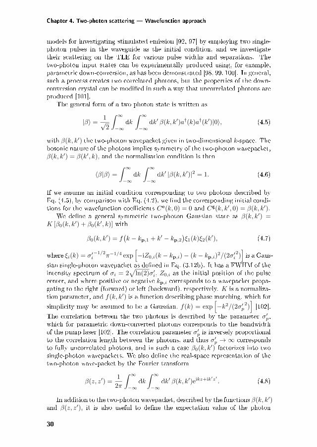
Chapter 4. Two-photon scattering — Wavefunction approach
models for investigating stimulated emission [92, 97] by employing two single-photon pulses in the waveguide as the initial condition, and we investigatetheir scattering on the TLE for various pulse widths and separations. Thetwo-photon input states can be experimentally produced using, for example,parametric down-conversion, as has been demonstrated [98, 99, 100]. In general,such a process creates two correlated photons, but the properties of the down-conversion crystal can be modified in such a way that uncorrelated photons areproduced [101].
The general form of a two-photon state is written as
|𝛽⟩ =1√2
∫ ∞
−∞d𝑘∫ ∞
−∞d𝑘′ 𝛽(𝑘, 𝑘′)𝑎†(𝑘)𝑎†(𝑘′)|0⟩, (4.5)
with 𝛽(𝑘, 𝑘′) the two-photon wavepacket given in two-dimensional 𝑘-space. Thebosonic nature of the photons implies symmetry of the two-photon wavepacket,𝛽(𝑘, 𝑘′) = 𝛽(𝑘′, 𝑘), and the normalisation condition is then
⟨𝛽|𝛽⟩ =
∫ ∞
−∞d𝑘∫ ∞
−∞d𝑘′ |𝛽(𝑘, 𝑘′)|2 = 1. (4.6)
If we assume an initial condition corresponding to two photons described byEq. (4.5), by comparison with Eq. (4.2), we find the corresponding initial condi-tions for the wavefunction coefficients 𝐶e(𝑘, 0) = 0 and 𝐶g(𝑘, 𝑘′, 0) = 𝛽(𝑘, 𝑘′).
We define a general symmetric two-photon Gaussian state as 𝛽(𝑘, 𝑘′) =𝐾 [𝛽0(𝑘, 𝑘′) + 𝛽0(𝑘′, 𝑘)] with
𝛽0(𝑘, 𝑘′) = 𝑓(𝑘 − 𝑘p,1 + 𝑘′ − 𝑘p,2
)𝜉1(𝑘)𝜉2(𝑘′), (4.7)
where 𝜉𝑖(𝑘) = 𝜎′𝑖−1/2
𝜋−1/4 exp[−i𝑍0,𝑖(𝑘 − 𝑘p,𝑖) − (𝑘 − 𝑘p,𝑖)
2/(2𝜎′𝑖2)]is a Gaus-
sian single-photon wavepacket as defined in Eq. (3.12b). It has a FWHM of theintensity spectrum of 𝜎𝑖 = 2
√ln(2)𝜎′
𝑖, 𝑍0,𝑖 as the initial position of the pulsecenter, and where positive or negative 𝑘p,𝑖 corresponds to a wavepacket propa-gating to the right (forward) or left (backward), respectively. 𝐾 is a normaliza-tion parameter, and 𝑓(𝑘, 𝑘′) is a function describing phase matching, which for
simplicity may be assumed to be a Gaussian, 𝑓(𝑘) = exp[−𝑘2/(2𝜎′
𝑝2)][102].
The correlation between the two photons is described by the parameter 𝜎′𝑝,
which for parametric down-converted photons corresponds to the bandwidthof the pump laser [102]. The correlation parameter 𝜎′
𝑝 is inversely proportionalto the correlation length between the photons, and thus 𝜎′
𝑝 → ∞ correspondsto fully uncorrelated photons, and in such a case 𝛽0(𝑘, 𝑘′) factorizes into twosingle-photon wavepackets. We also define the real-space representation of thetwo-photon wave-packet by the Fourier transform
𝛽(𝑧, 𝑧′) =1
2𝜋
∫ ∞
−∞d𝑘∫ ∞
−∞d𝑘′ 𝛽(𝑘, 𝑘′)ei𝑘𝑧+i𝑘′𝑧′
. (4.8)
In addition to the two-photon wavepacket, described by the functions 𝛽(𝑘, 𝑘′)and 𝛽(𝑧, 𝑧′), it is also useful to define the expectation value of the photon
30
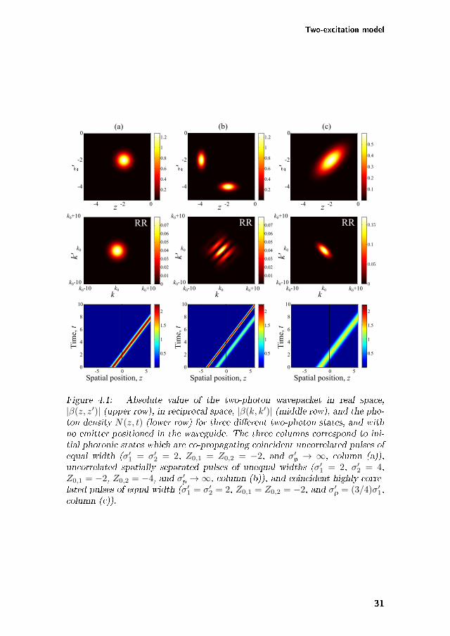
Two-excitation model
0
0.05
0.1
0.15RR
0.1
0.2
0.3
0.4
0.5
0
0.01
0.02
0.03
0.04
0.05
0.06
0.07
0.2
0.4
0.6
0.8
1
1.2
(a)
0-5 0 5
2
4
6
8
10
0.5
1
1.5
2
Tim
e, t
Spatial position, z Spatial position, z
Tim
e, t
(b) (c)
Spatial position, z
Tim
e, t
-4 -2 0
-4
-2
0
z
z'
k0
k0+10
k
k'
k0-10k0+10k0k0-10
0.2
0.4
0.6
0.8
1
1.2
0.01
0.02
0.03
0.04
0.05
0.06
0.07
0-5 0 5
2
4
6
8
10
0.5
1
1.5
2
0-5 0 5
2
4
6
8
10
-4 -2 0
-4
-2
0
z
z'
k0
k0+10
k
k'
k0-10k0+10k0k0-10
-4 -2 0
-4
-2
0
z
z'
k0
k0+10
k
k'
k0-10k0+10k0k0-10
RR RR
0.5
1
1.5
2
Figure 4.1: Absolute value of the two-photon wavepacket in real space,|𝛽(𝑧, 𝑧′)| (upper row), in reciprocal space, |𝛽(𝑘, 𝑘′)| (middle row), and the pho-ton density 𝑁(𝑧, 𝑡) (lower row) for three different two-photon states, and withno emitter positioned in the waveguide. The three columns correspond to ini-tial photonic states which are co-propagating coincident uncorrelated pulses ofequal width (𝜎′
1 = 𝜎′2 = 2, 𝑍0,1 = 𝑍0,2 = −2, and 𝜎′
p → ∞, column (a)),uncorrelated spatially separated pulses of unequal widths (𝜎′
1 = 2, 𝜎′2 = 4,
𝑍0,1 = −2, 𝑍0,2 = −4, and 𝜎′p → ∞, column (b)), and coincident highly corre-
lated pulses of equal width (𝜎′1 = 𝜎′
2 = 2, 𝑍0,1 = 𝑍0,2 = −2, and 𝜎′p = (3/4)𝜎′
1,column (c)).
31
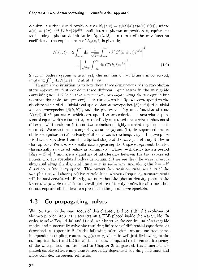
Chapter 4. Two-photon scattering — Wavefunction approach
density at a time 𝑡 and position 𝑧 as 𝑁𝑧(𝑧, 𝑡) = ⟨𝜓(𝑡)|𝑎†(𝑧)𝑎(𝑧)|𝜓(𝑡)⟩, where𝑎(𝑧) = (2𝜋)−1/2
∫d𝑘 𝑎(𝑘)ei𝑘𝑧 annihilates a photon at position 𝑧, equivalent
to the single-photon definition in Eq. (3.15). In terms of the wavefunctioncoefficients, the explicit form of 𝑁𝑧(𝑧, 𝑡) is given by
𝑁𝑧(𝑧, 𝑡) = 2
∫ ∞
−∞d𝑘
1√2𝜋
∫ ∞
−∞d𝑘′ 𝐶g(𝑘, 𝑘′, 𝑡)ei𝑘
′𝑧
2+
1√2𝜋
∫ ∞
−∞d𝑘 𝐶e(𝑘, 𝑡)ei𝑘𝑧
2. (4.9)
Since a lossless system is assumed, the number of excitations is conserved,implying
∫∞−∞ d𝑧 𝑁(𝑧, 𝑡) = 2 at all times.
To gain some intuition as to how these three descriptions of the two-photonstate appear, we first consider three different input states in the waveguidecontaining no TLE (such that wavepackets propagate along the waveguide butno other dynamics are present). The three rows in Fig. 4.1 correspond to theabsolute value of the initial real-space photon wavepacket |𝛽(𝑧, 𝑧′)|, the initial𝑘-space wavepacket |𝛽(𝑘, 𝑘′)|, and the photon density as a function of time𝑁(𝑧, 𝑡), for input states which correspond to two coincident uncorrelated pho-tons of equal width column (a), two spatially separated uncorrelated photons ofdifferent width column (b), and two coincident highly-correlated photons col-umn (c). We note that in comparing columns (a) and (b), the separated natureof the two pulses in (b) is clearly visible, as too is the inequality of the two pulsewidths, as is evident from the elliptical shape of the wavepactet amplitudes inthe top row. We also see oscillations appearing the 𝑘-space representation forthe spatially separated pulses in column (b). These oscillations have a period|𝑍0,1 − 𝑍0,2|−1 and are a signature of interference between the two separatedpulses. For the correlated pulses in column (c) we see that the wavepacket iselongated along the diagonal line 𝑧 = 𝑧′ in real-space, and along the 𝑘 = −𝑘′direction in frequency space. This means that position measurements of thetwo photons will share positive correlations, whereas frequency measurementswill be anti-correlated. Finally, we note that the photon density plots in thelower row provide us with an overall picture of the dynamics for all times, butdo not capture all the features present in the photon wavepackets.
4.3 Co-propagating pulses
We now turn to the main focus of this chapter, and consider the evolution ofthe two photon state as it scatters on a TLE placed inside the waveguide. Inorder to solve Eqs. (4.4a) and (4.4b), we discretize the continuum of waveguidemodes and numerically solve the resulting finite set of differential equations, asdescribed in Appendix B. In the following calculations we assume frequency-independent coupling constants, 𝑔(𝑘) = 𝑔, which is well justified owing to theassumption that the TLE linewidth is narrow compared to the carrier frequencyof the wavepackets, as discussed in Chapter 3; in general, the numerical ap-proach employed here may handle frequency dependent coupling constants andmore complex dispersion relations.
32
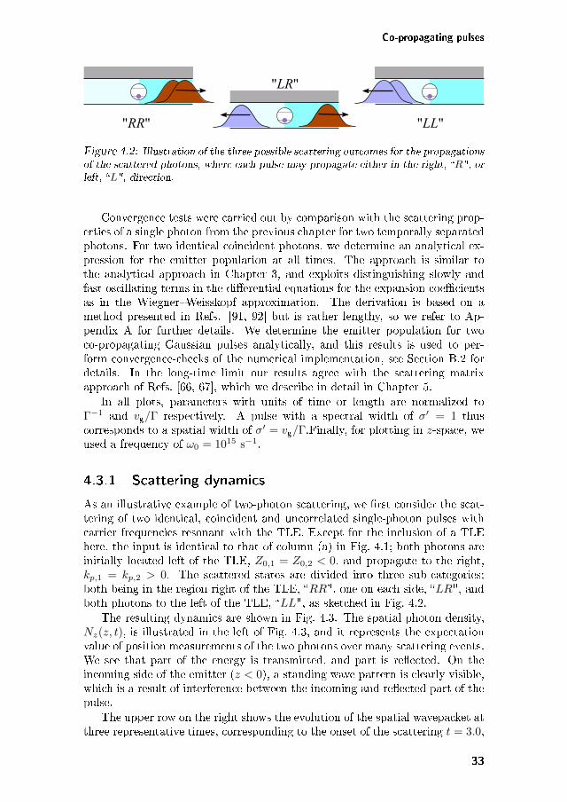
Co-propagating pulses
"LR"
"RR" "LL"
Figure 4.2: Illustration of the three possible scattering outcomes for the propagationsof the scattered photons, where each pulse may propagate either in the right, “𝑅", orleft, “𝐿", direction.
Convergence tests were carried out by comparison with the scattering prop-erties of a single photon from the previous chapter for two temporally separatedphotons. For two identical coincident photons, we determine an analytical ex-pression for the emitter population at all times. The approach is similar tothe analytical approach in Chapter 3, and exploits distinguishing slowly andfast oscillating terms in the differential equations for the expansion coefficientsas in the Wiegner–Weisskopf approximation. The derivation is based on amethod presented in Refs. [91, 92] but is rather lengthy, so we refer to Ap-pendix A for further details. We determine the emitter population for twoco-propagating Gaussian pulses analytically, and this results is used to per-form convergence-checks of the numerical implementation, see Section B.2 fordetails. In the long-time limit our results agree with the scattering matrixapproach of Refs. [66, 67], which we describe in detail in Chapter 5.
In all plots, parameters with units of time or length are normalized toΓ−1 and 𝑣g/Γ respectively. A pulse with a spectral width of 𝜎′ = 1 thuscorresponds to a spatial width of 𝜎′ = 𝑣g/Γ.Finally, for plotting in 𝑧-space, weused a frequency of 𝜔0 = 1015 s−1.
4.3.1 Scattering dynamics
As an illustrative example of two-photon scattering, we first consider the scat-tering of two identical, coincident and uncorrelated single-photon pulses withcarrier frequencies resonant with the TLE. Except for the inclusion of a TLEhere, the input is identical to that of column (a) in Fig. 4.1; both photons areinitially located left of the TLE, 𝑍0,1 = 𝑍0,2 < 0, and propagate to the right,𝑘𝑝,1 = 𝑘𝑝,2 > 0. The scattered states are divided into three sub-categories:both being in the region right of the TLE, “𝑅𝑅", one on each side, “𝐿𝑅", andboth photons to the left of the TLE, “𝐿𝐿", as sketched in Fig. 4.2.
The resulting dynamics are shown in Fig. 4.3. The spatial photon density,𝑁𝑧(𝑧, 𝑡), is illustrated in the left of Fig. 4.3, and it represents the expectationvalue of position measurements of the two photons over many scattering events.We see that part of the energy is transmitted, and part is reflected. On theincoming side of the emitter (𝑧 < 0), a standing wave pattern is clearly visible,which is a result of interference between the incoming and reflected part of thepulse.
The upper row on the right shows the evolution of the spatial wavepacket atthree representative times, corresponding to the onset of the scattering 𝑡 = 3.0,
33
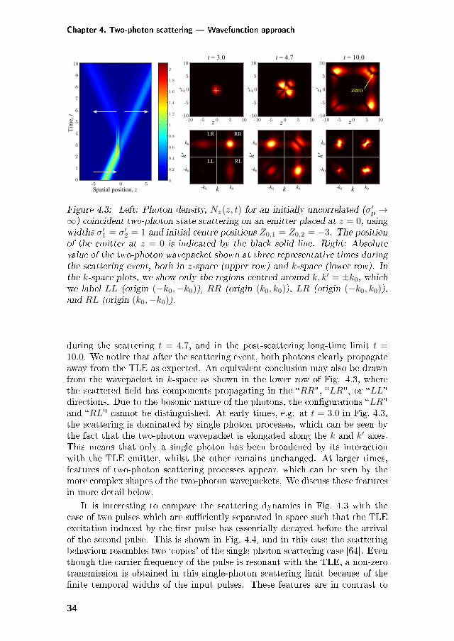
Chapter 4. Two-photon scattering — Wavefunction approach
Tim
e, t
t = 10.0
zero
kk0-k0
t = 4.7
-10 -5 0 5 10-10
-5
0
5
10
z'
k
k'
-k0
k0
k0-k0
-10 -5 0 5 10-10
-5
0
5
10
z'
k
k'
-k0
k0
k0-k0
z
t = 3.0
-10 -5 0 5 10-10
-5
0
5
10
z'
k'
-k0
k0
RR
RLLL
LR
-5 0 50
0.2
0.4
0.6
0.8
1
1.2
1.4
1.6
1.8
2
0
1
2
3
4
5
6
7
8
9
10T
ime,
t
Spatial position, z
z z
Figure 4.3: Left: Photon density, 𝑁𝑧(𝑧, 𝑡) for an initially uncorrelated (𝜎′p →
∞) coincident two-photon state scattering on an emitter placed at 𝑧 = 0, usingwidths 𝜎′
1 = 𝜎′2 = 1 and initial centre positions 𝑍0,1 = 𝑍0,2 = −3. The position
of the emitter at 𝑧 = 0 is indicated by the black solid line. Right: Absolutevalue of the two-photon wavepacket shown at three representative times duringthe scattering event, both in 𝑧-space (upper row) and 𝑘-space (lower row). Inthe 𝑘-space plots, we show only the regions centred around 𝑘, 𝑘′ = ±𝑘0, whichwe label 𝐿𝐿 (origin (−𝑘0,−𝑘0)), 𝑅𝑅 (origin (𝑘0, 𝑘0)), 𝐿𝑅 (origin (−𝑘0, 𝑘0)),and 𝑅𝐿 (origin (𝑘0,−𝑘0)).
during the scattering 𝑡 = 4.7, and in the post-scattering long-time limit 𝑡 =10.0. We notice that after the scattering event, both photons clearly propagateaway from the TLE as expected. An equivalent conclusion may also be drawnfrom the wavepacket in 𝑘-space as shown in the lower row of Fig. 4.3, wherethe scattered field has components propagating in the “𝑅𝑅", “𝐿𝑅", or “𝐿𝐿"directions. Due to the bosonic nature of the photons, the configurations “𝐿𝑅"and “𝑅𝐿" cannot be distinguished. At early times, e.g. at 𝑡 = 3.0 in Fig. 4.3,the scattering is dominated by single photon processes, which can be seen bythe fact that the two-photon wavepacket is elongated along the 𝑘 and 𝑘′ axes.This means that only a single photon has been broadened by its interactionwith the TLE emitter, whilst the other remains unchanged. At larger times,features of two-photon scattering processes appear, which can be seen by themore complex shapes of the two-photon wavepackets. We discuss these featuresin more detail below.
It is interesting to compare the scattering dynamics in Fig. 4.3 with thecase of two pulses which are sufficiently separated in space such that the TLEexcitation induced by the first pulse has essentially decayed before the arrivalof the second pulse. This is shown in Fig. 4.4, and in this case the scatteringbehaviour resembles two ‘copies’ of the single-photon scattering case [64]. Eventhough the carrier frequency of the pulse is resonant with the TLE, a non-zerotransmission is obtained in this single-photon scattering limit because of thefinite temporal widths of the input pulses. These features are in contrast to
34
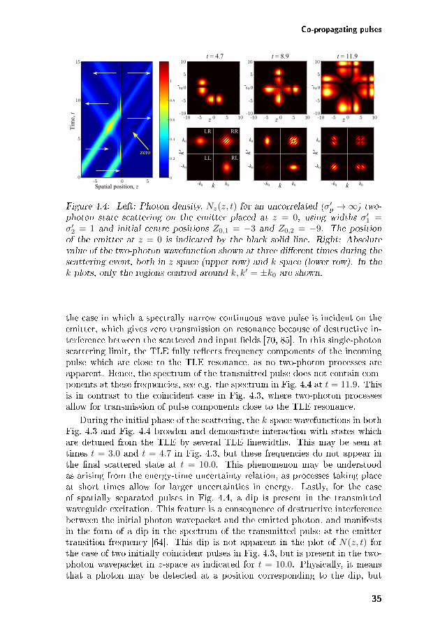
Co-propagating pulses
t = 4.7 t = 8.9 t = 11.9
-10 -5 0 5 10-10
-5
0
5
10
z'
kk'
-k0
k0
k0-k0
-10 -5 0 5 10-10
-5
0
5
10
z'
k
k'
-k0
k0
k0-k0
-10 -5 0 5 10-10
-5
0
5
10
z'
k
k'
-k0
k0
k0-k0
RR
RLLL
LR
Spatial position, z
Tim
e, t
-5 0 50
5
10
15
0
0.2
0.4
0.6
0.8
1
zero
z z z
Figure 4.4: Left: Photon density, 𝑁𝑧(𝑧, 𝑡) for an uncorrelated (𝜎′p → ∞) two-
photon state scattering on the emitter placed at 𝑧 = 0, using widths 𝜎′1 =
𝜎′2 = 1 and initial centre positions 𝑍0,1 = −3 and 𝑍0,2 = −9. The position
of the emitter at 𝑧 = 0 is indicated by the black solid line. Right: Absolutevalue of the two-photon wavefunction shown at three different times during thescattering event, both in 𝑧-space (upper row) and 𝑘-space (lower row). In the𝑘-plots, only the regions centred around 𝑘, 𝑘′ = ±𝑘0 are shown.
the case in which a spectrally narrow continuous wave pulse is incident on theemitter, which gives zero transmission on resonance because of destructive in-terference between the scattered and input fields [70, 85]. In this single-photonscattering limit, the TLE fully reflects frequency components of the incomingpulse which are close to the TLE resonance, as no two-photon processes areapparent. Hence, the spectrum of the transmitted pulse does not contain com-ponents at these frequencies, see e.g. the spectrum in Fig. 4.4 at 𝑡 = 11.9. Thisis in contrast to the coincident case in Fig. 4.3, where two-photon processesallow for transmission of pulse components close to the TLE resonance.
During the initial phase of the scattering, the 𝑘-space wavefunctions in bothFig. 4.3 and Fig. 4.4 broaden and demonstrate interaction with states whichare detuned from the TLE by several TLE linewidths. This may be seen attimes 𝑡 = 3.0 and 𝑡 = 4.7 in Fig. 4.3, but these frequencies do not appear inthe final scattered state at 𝑡 = 10.0. This phenomenon may be understoodas arising from the energy-time uncertainty relation, as processes taking placeat short times allow for larger uncertainties in energy. Lastly, for the caseof spatially separated pulses in Fig. 4.4, a dip is present in the transmittedwaveguide excitation. This feature is a consequence of destructive interferencebetween the initial photon wavepacket and the emitted photon, and manifestsin the form of a dip in the spectrum of the transmitted pulse at the emittertransition frequency [64]. This dip is not apparent in the plot of 𝑁(𝑧, 𝑡) forthe case of two initially coincident pulses in Fig. 4.3, but is present in the two-photon wavepacket in 𝑧-space as indicated for 𝑡 = 10.0. Physically, it meansthat a photon may be detected at a position corresponding to the dip, but
35
Chapter 4. Two-photon scattering — Wavefunction approach
if the first photon is detected there, the probability of detecting the secondphoton at that position is zero, exemplifying that the single-photon scatteringfeatures manifest themselves in two-photon scattering, although they may notbe apparent from the photon density 𝑁(𝑧, 𝑡).
To summarise, we have illustrated the full scattering dynamics of two pho-tons on a TLE by calculating the total system state at all times. For well-separated uncorrelated single-photon pulses, the dynamics may be well ap-proximated by the single-photon results [64]. As the displacement between thepulses becomes smaller, non-trivial dynamics can be induced due to the sat-uration of the TLE. The approach we use here naturally accommodates thisregime of two photon scattering.
4.3.2 Transmission and reflection properties
In order to investigate the transmission properties of the TLE, we considerthe relative number of photons propagating to the left and right during thescattering process. We can calculate the total number of photons propagatingto the right as
𝑁R(𝑡) =
∫ ∞
0
d𝑘 ⟨𝜓(𝑡)|𝑎†(𝑘)𝑎(𝑘)|𝜓(𝑡)⟩ (4.10)
= 2
∫ ∞
0
d𝑘
∫ ∞
−∞d𝑘′ |𝐶g(𝑘, 𝑘′, 𝑡)|2 +
∫ ∞
0
d𝑘 |𝐶e(𝑘, 𝑡)|2, (4.11)
while the total number propagating to the left, is given by a similar expressionwith the integration range over 𝑘 changed to ] −∞, 0],
𝑁L(𝑡) =
∫ 0
−∞d𝑘 ⟨𝜓(𝑡)|𝑎†(𝑘)𝑎(𝑘)|𝜓(𝑡)⟩. (4.12)
The excitation probability of the TLE is given by
𝑃e(𝑡) = ⟨𝜓(𝑡)|𝑐†𝑐|𝜓(𝑡)⟩ =
∫ ∞
−∞d𝑘𝐶e(𝑘, 𝑡)
2, (4.13)
and normalization of the total state ensures 𝑁R(𝑡) + 𝑁L(𝑡) + 𝑃e(𝑡) = 2; thereis a total of two excitations in the system at all times. We therefore definethe relative transmission to the right and left as 𝑇R(𝑡) = 𝑁R(𝑡)/2 and 𝑇L(𝑡) =𝑁L(𝑡)/2.
In Fig. 4.5(a) we show the left and right transmission coefficients, togetherwith the TLE excitation as a function of time, for the two cases of perfectlyoverlapping (solid) and non-overlapping pulses (dashed) introduced in Figs. 4.3and 4.4 respectively. From these plots a clear reduction in the reflective natureof the TLE when the two pulses are coincident is evident, clearly illustratingthat the first photon induces partial transparency in the TLE, minimising theinteraction between the TLE and the second photon1. Also evident is a tempo-ral delay between excitation of the TLE and the accumulation of the reflected
1Due to the symmetry, the maximum achievable TLE excitation for a single-pulse excita-tion from a single side is 1/2, as discussed with Fig. 3.2(b). A value of 1/2 is only obtainedfor a pulse with a temporal shape which is exactly the inverse of a pulse emitted by theTLE [103]. Such a pulse would render the TLE completely transparent.
36
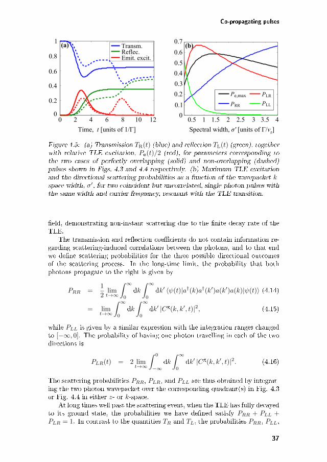
Co-propagating pulses
Transm.Reflec.Emit.4excit.
Pe,max
PRR
PLR
PLL
Spectral4width,4σ'4[units4of4Γ/vg]Time,44t4[units4of41/Γ]
0
0.2
0.4
0.6
0.8
1
0 2 4 6 8 10 12
0.7
0.6
0.5
0.4
0.3
0.2
0.1
00.5 1 1.5 2 32.5 3.5 4
(a) (b)
Figure 4.5: (a) Transmission 𝑇R(𝑡) (blue) and reflection 𝑇L(𝑡) (green), togetherwith relative TLE excitation, 𝑃e(𝑡)/2 (red), for parameters corresponding tothe two cases of perfectly overlapping (solid) and non-overlapping (dashed)pulses shown in Figs. 4.3 and 4.4 respectively. (b) Maximum TLE excitationand the directional scattering probabilities as a function of the wavepacket 𝑘-space width, 𝜎′, for two coincident but uncorrelated, single-photon pulses withthe same width and carrier frequency, resonant with the TLE transition.
field, demonstrating non-instant scattering due to the finite decay rate of theTLE.
The transmission and reflection coefficients do not contain information re-garding scattering-induced correlations between the photons, and to that endwe define scattering probabilities for the three possible directional outcomesof the scattering process. In the long-time limit, the probability that bothphotons propagate to the right is given by
𝑃𝑅𝑅 =1
2lim𝑡→∞
∫ ∞
0
d𝑘∫ ∞
0
d𝑘′ ⟨𝜓(𝑡)|𝑎†(𝑘)𝑎†(𝑘′)𝑎(𝑘′)𝑎(𝑘)|𝜓(𝑡)⟩ (4.14)
= lim𝑡→∞
∫ ∞
0
d𝑘∫ ∞
0
d𝑘′ |𝐶g(𝑘, 𝑘′, 𝑡)|2, (4.15)
while 𝑃𝐿𝐿 is given by a similar expression with the integration ranges changedto [−∞, 0]. The probability of having one photon travelling in each of the twodirections is
𝑃𝐿𝑅(𝑡) = 2 lim𝑡→∞
∫ 0
−∞d𝑘∫ ∞
0
d𝑘′ |𝐶g(𝑘, 𝑘′, 𝑡)|2. (4.16)
The scattering probabilities 𝑃𝑅𝑅, 𝑃𝐿𝑅, and 𝑃𝐿𝐿 are thus obtained by integrat-ing the two-photon wavepacket over the corresponding quadrant(s) in Fig. 4.3or Fig. 4.4 in either 𝑧- or 𝑘-space.
At long times well past the scattering event, when the TLE has fully decayedto its ground state, the probabilities we have defined satisfy 𝑃𝑅𝑅 + 𝑃𝐿𝐿 +𝑃𝐿𝑅 = 1. In contrast to the quantities 𝑇𝑅 and 𝑇𝐿, the probabilities 𝑃𝑅𝑅, 𝑃𝐿𝐿,
37
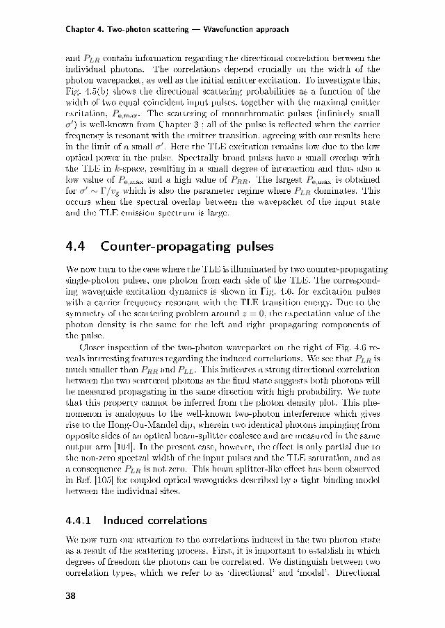
Chapter 4. Two-photon scattering — Wavefunction approach
and 𝑃𝐿𝑅 contain information regarding the directional correlation between theindividual photons. The correlations depend crucially on the width of thephoton wavepacket, as well as the initial emitter excitation. To investigate this,Fig. 4.5(b) shows the directional scattering probabilities as a function of thewidth of two equal coincident input pulses, together with the maximal emitterexcitation, 𝑃e,max. The scattering of monochromatic pulses (infinitely small𝜎′) is well-known from Chapter 3 ; all of the pulse is reflected when the carrierfrequency is resonant with the emitter transition, agreeing with our results herein the limit of a small 𝜎′. Here the TLE excitation remains low due to the lowoptical power in the pulse. Spectrally broad pulses have a small overlap withthe TLE in 𝑘-space, resulting in a small degree of interaction and thus also alow value of 𝑃e,max and a high value of 𝑃𝑅𝑅. The largest 𝑃e,max is obtainedfor 𝜎′ ∼ Γ/𝑣g which is also the parameter regime where 𝑃𝐿𝑅 dominates. Thisoccurs when the spectral overlap between the wavepacket of the input stateand the TLE emission spectrum is large.
4.4 Counter-propagating pulses
We now turn to the case where the TLE is illuminated by two counter-propagatingsingle-photon pulses, one photon from each side of the TLE. The correspond-ing waveguide excitation dynamics is shown in Fig. 4.6, for excitation pulseswith a carrier frequency resonant with the TLE transition energy. Due to thesymmetry of the scattering problem around 𝑧 = 0, the expectation value of thephoton density is the same for the left and right propagating components ofthe pulse.
Closer inspection of the two-photon wavepacket on the right of Fig. 4.6 re-veals interesting features regarding the induced correlations. We see that 𝑃𝐿𝑅 ismuch smaller than 𝑃𝑅𝑅 and 𝑃𝐿𝐿. This indicates a strong directional correlationbetween the two scattered photons as the final state suggests both photons willbe measured propagating in the same direction with high probability. We notethat this property cannot be inferred from the photon density plot. This phe-nomenon is analogous to the well-known two-photon interference which givesrise to the Hong-Ou-Mandel dip, wherein two identical photons impinging fromopposite sides of an optical beam-splitter coalesce and are measured in the sameoutput arm [104]. In the present case, however, the effect is only partial due tothe non-zero spectral width of the input pulses and the TLE saturation, and asa consequence 𝑃𝐿𝑅 is not zero. This beam splitter-like effect has been observedin Ref. [105] for coupled optical waveguides described by a tight-binding modelbetween the individual sites.
4.4.1 Induced correlations
We now turn our attention to the correlations induced in the two-photon-stateas a result of the scattering process. First, it is important to establish in whichdegrees of freedom the photons can be correlated. We distinguish between twocorrelation types, which we refer to as ‘directional’ and ‘modal’. Directional
38
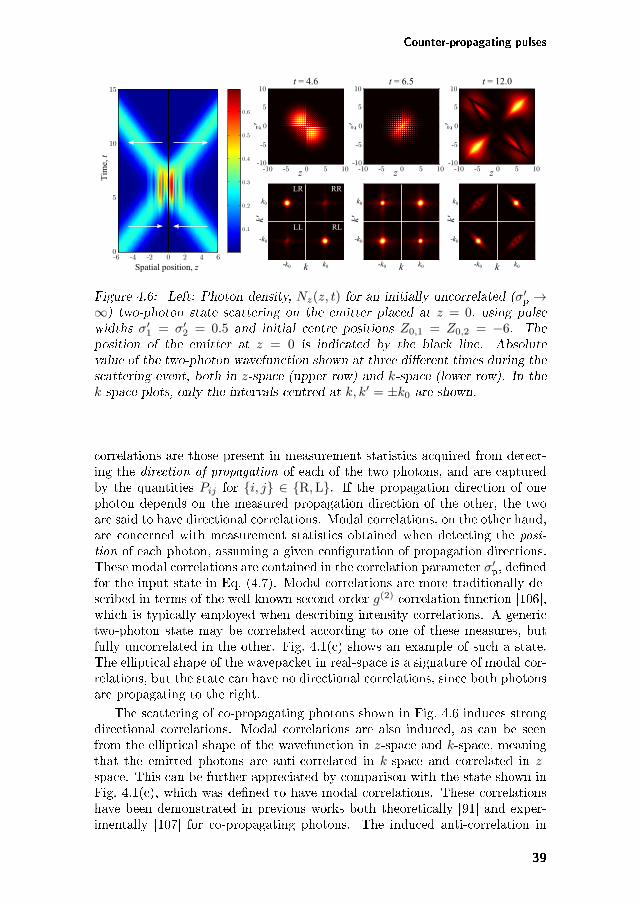
Counter-propagating pulses
t = 4.6 t = 6.5
-10 -5 0 5 10-10
-5
0
5
10
z'
kk'
-k0
k0
k0-k0
-10 -5 0 5 10-10
-5
0
5
10
z'
k
k'
-k0
k0
k0-k0
t = 12.0
-10 -5 0 5 10-10
-5
0
5
10
z'
k
k'
-k0
k0
k0-k0
RR
RLLL
LR
Spatial position, z
Tim
e, t
-6 -4 -2 0 2 4 60
5
10
15
0.1
0.2
0.3
0.4
0.5
0.6
z z z
Figure 4.6: Left: Photon density, 𝑁𝑧(𝑧, 𝑡) for an initially uncorrelated (𝜎′p →
∞) two-photon state scattering on the emitter placed at 𝑧 = 0, using pulsewidths 𝜎′
1 = 𝜎′2 = 0.5 and initial centre positions 𝑍0,1 = 𝑍0,2 = −6. The
position of the emitter at 𝑧 = 0 is indicated by the black line. Absolutevalue of the two-photon wavefunction shown at three different times during thescattering event, both in 𝑧-space (upper row) and 𝑘-space (lower row). In the𝑘-space plots, only the intervals centred at 𝑘, 𝑘′ = ±𝑘0 are shown.
correlations are those present in measurement statistics acquired from detect-ing the direction of propagation of each of the two photons, and are capturedby the quantities 𝑃𝑖𝑗 for 𝑖, 𝑗 ∈ R,L. If the propagation direction of onephoton depends on the measured propagation direction of the other, the twoare said to have directional correlations. Modal correlations, on the other hand,are concerned with measurement statistics obtained when detecting the posi-tion of each photon, assuming a given configuration of propagation directions.These modal correlations are contained in the correlation parameter 𝜎′
p, definedfor the input state in Eq. (4.7). Modal correlations are more traditionally de-scribed in terms of the well-known second order 𝑔(2) correlation function [106],which is typically employed when describing intensity correlations. A generictwo-photon state may be correlated according to one of these measures, butfully uncorrelated in the other. Fig. 4.1(c) shows an example of such a state.The elliptical shape of the wavepacket in real-space is a signature of modal cor-relations, but the state can have no directional correlations, since both photonsare propagating to the right.
The scattering of co-propagating photons shown in Fig. 4.6 induces strongdirectional correlations. Modal correlations are also induced, as can be seenfrom the elliptical shape of the wavefunction in 𝑧-space and 𝑘-space, meaningthat the emitted photons are anti-correlated in 𝑘-space and correlated in 𝑧-space. This can be further appreciated by comparison with the state shown inFig. 4.1(c), which was defined to have modal correlations. These correlationshave been demonstrated in previous works both theoretically [91] and exper-imentally [107] for co-propagating photons. The induced anti-correlation in
39
Chapter 4. Two-photon scattering — Wavefunction approach
𝑘-space can be understood as a four-wave mixing process, where elastic scat-tering of two photons of almost identical energy results in one photon withhigher energy and one with lower energy. This gives rise to the elliptical shapeof the wavefunction in 𝑘-space, cf. the spectrum in Fig. 4.6 at 𝑡 = 12.0. Thecorrelation in 𝑧-space implies a larger probability of detecting the second pho-ton spatially close to the first, i.e. photon bunching. Modal correlations suchas these are not present in the scattered state from a conventional linear opticalbeam splitter; the modal entanglement observed here is caused by a non-linearscattering process between the incoming and emitted photons, which is medi-ated by the excitation of the TLE.
In order to relate the induced quantum correlations in the photonic stateto the TLE excitation dynamics, we require a measure of the induced cor-relations, which can be facilitated by entanglement theory. There are severalproposals in the literature of how to quantify the degree of entanglement (quan-tum correlations) between individual subsystems [108, 109, 110], particularlyfor distinguishable systems each of which may be in one of only two states,e.g. two spatially separated spin-half particles. These measures include thefidelity, the concurrence, the negativity, and the entropy of entanglement [38],each of which has a different operational meaning, and may be more or lessappropriate given the problem at hand. For two indistinguishable particles e.g.two bosons in the same two-photon Hilbert space, extensions to the distin-guishable case have to be made [111, 112, 113]. If the indistinguishable bosonscan each occupy more than two states, as is the case for the state expressedby Eq. (4.5) (where the number of states is equal to the dimension of eachparticle sub-Hilbert space), there are fewer ways to quantify the entanglement.Among these is the von Neumann entropy of the reduced single-particle densitymatrix [112, 114], which quantifies the modal entanglement by the degree towhich the state of the second photon is affected by a 𝑘-space measurement onthe first.
In order to explore the extent to which our system behaves as a beam-splitter, we quantify the amount of directional entanglement present in thescattered state. To do this, the two-photon state may be projected onto atwo-dimensional Hilbert space with each photon being in either a left or aright propagating state, giving three basis states, |𝐿𝐿⟩, |𝐿𝑅⟩, and |𝑅𝑅⟩. Thisprojected system is identical to the case of two indistinguishable two-stateparticles discussed above, for which the entanglement may be quantified by thefidelity, i.e. by comparison to a maximally entangled state. We focus here onlyon entangled states with a different number of particles in each direction andthus compare to two of the four Bell-states only,
|Φ±⟩ =1√2
[|𝐿𝐿⟩ ± |𝑅𝑅⟩] . (4.17)
Here |𝐿𝐿⟩ and |𝑅𝑅⟩ are states with the same modal correlations as the partsof the calculated scattered state where both photons propagate to the left orboth to the right, respectively. For pure states as in Eq. (4.5), the fidelitieswith respect to the maximally entangled states projected onto the |𝐿⟩ and |𝑅⟩basis are defined as the overlap between the scattered state and the maximally
40
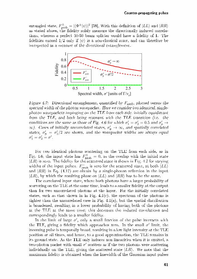
Counter-propagating pulses
entangled state, 𝐹±prob = |⟨Φ±|𝜓⟩|2 [38], With this definition of |𝐿𝐿⟩ and |𝑅𝑅⟩
as stated above, the fidelity solely measure the directionally induced correla-tions, whereas a perfect 50-50 beam splitter would have a fidelity of 1. Thefidelities exceed 1/2 only if |𝜓⟩ is a non-classical state, and can therefore beinterpreted as a measure of the directional entanglement.
0.5 1 1.5 2 2.5 30
0.2
0.4
0.6
0.8
1
Fprob
+
Fprob
-
Spectral/width,/σ'/[units/of/Γ/vg]/
Fid
elit
yσp ∞
σp =/σ ///2/' '
'
Figure 4.7: Directional entanglement, quantified by 𝐹prob, plotted versus thespectral width of the photon wavepacket. Here we consider two identical, single-photon wavepackets impinging on the TLE from each side, initially equidistantfrom the TLE, and both being resonant with the TLE transition (i.e. theconditions are the same as those of Fig. 4.6 for which 𝜎′
1 = 𝜎′2 = 0.5 and 𝜎′
𝑝 →∞). Cases of initially uncorrelated states, 𝜎′
p → ∞, and spatially correlatedstates, 𝜎′
p = 𝜎′1/2 are shown, and the wavepacket widths are always equal
𝜎′1 = 𝜎′
2 = 𝜎′.
For two identical photons scattering on the TLE from each side, as inFig. 4.6, the input state has 𝐹±
prob = 0, as the overlap with the initial state|𝐿𝑅⟩ is zero. The fidelity for the scattered state is shown in Fig. 4.7 for varyingwidths of the input pulses. 𝐹−
prob is zero for the scattered state, at both |𝐿𝐿⟩and |𝑅𝑅⟩ in Eq. (4.17) are obtain by a single-photon reflection in the input|𝐿𝑅⟩, by which the resulting phase on |𝐿𝐿⟩ and |𝑅𝑅⟩ has to be the same.
The correlated input state, where both photons have a larger probability ofscattering on the TLE at the same time, leads to a smaller fidelity at the outputthan for two uncorrelated photons at the input. For the initially correlatedstates, such as that shown in in Fig. 4.1(c), the spectrum of the photons istighter than the uncorrelated case in Fig. 4.1(a), but the spatial distributionis broadened, resulting in a lower probability of having both of the photonsat the TLE at the same time; this decreases the induced correlations andcorrespondingly leads to a smaller fidelity.
In the limit of large 𝜎′, only a small fraction of the pulse interacts withthe TLE, giving a fidelity which approaches zero. In the small 𝜎′ limit, theincoming pulse is temporally broad, resulting in a low light intensity at the TLEposition at all times, and hence, to a good approximation, the TLE remains inits ground state. As the TLE only induces non-linearities when it is excited, atwo-photon packet with small 𝜎′ scatters as if the two photons were scatteringindividually on the TLE, giving the scattered state |𝐿𝑅⟩. We note that themaximum fidelity is obtained when the linewidth of the Gaussian input pulses
41
Chapter 4. Two-photon scattering — Wavefunction approach
is comparable with the decay rate of the TLE, i.e. for full-width half maximumof the incoming pulse on the order 𝜎 = 2
√ln(2)𝜎′ ≈ 1.0. In this case excitation
of the TLE is high, and a highly directionally entangled state is produced.
4.5 Summary
In conclusion, we have developed a wavefunction approach to study the scat-tering of two photons on a two-level emitter in a one-dimensional waveguide.Our method benefits from the simple mathematical form, and provides thefull temporal dynamics of the scattering event, as well as a detailed descrip-tion of the scattering-induced correlations. For co-propagating pulses, we sawthat the excitation of the emitter strongly influences its transparency. This re-sults in transmission and reflection coefficients which depend sensitively on theseparation between the two input pulses. For counter-propagating pulses, theemitter–waveguide system shows beam-splitter like features, generating direc-tional correlations in the scattered two-photon state, occurring most stronglywhen the emitter excitation is largest. Unlike a conventional linear opticalbeam-splitter, however, the finite decay rate of the emitter introduces non-linearities which manifest as additional bunching effects. Finally, we note thatour model could be extended to more complicated scattering scenarios, suchas several quantum dots with possibly additional levels [115, 82, 116]. The nu-merical approach we use also allows for the investigation of the role of waveg-uide dispersion, as well as non-Markovian coupling to the scattering object byincluding frequency-dependent coupling coefficients in the system. Lastly, an-other strength of this numerical approach is the possibility of several, spatiallyseparated emitters. Other approaches such as the scattering matrix formalismbecomes very complex for two-photon scattering, due to recursive terms whereenergy may oscillate back and forth between the scatterers [116], which we planto look into in future studies.
42
Chapter 5
Two-photon scattering —
Scattering matrix approach
In this chapter we discuss another approach to analyse two-photon scattering ona non-linearity, namely the scattering matrix formalism. For typical scatteringexperiments where an input state is sent toward a scattering region, the problemis often treated mathematically by the scattering matrix formalism. The stateof the photon pulse long after the scattering process is related to the to theinitial state through the scattering matrix operator 𝑆, which is equal to theevolution operator in the interaction picture from time −∞ to ∞. For non-linear scatterers, the scattering matrix will in general be frequency dependent,and is given by
𝑆 = lim𝑡𝑖→−∞𝑡𝑒→∞
ei𝐻0𝑡𝑒e−i𝐻(𝑡𝑒−𝑡𝑖)e−i𝐻0𝑡𝑖 (5.1)
with 𝐻0 being the non-interaction part of the system Hamiltonian, 𝐻 [66].Thus, if the scattering matrix elements for a specific scatterer has been de-termined, the post-scattering may be determined using standard algebra. Itis, however, not trivial to determine the scattering matrix elements for few-photon non-linearities, due to possible non-linear scattering processes wherethe energy between multiple input photons may be changed, as demonstratedin the previous chapter.
The scattering elements may be determined by various methods, such asthe input-output formalism [66], the Bethe Ansatz [87, 88], and the Lehmann-Symanzik-Zimmermann formalism [89]. These approaches have been exploitedto calculate the scattering matrix elements for two-photon states in varioussystems such as a single emitter [66, 67], an emitter inside an optical cavi-tiy [117], an emitter coupled to a ring resonator [118], and a non-linear op-tical cavity [119]. In contrast to the numerical approach in Chapter 4, thescattering matrix calculations complicate when considering scatterers whichconsist of multiple elements, and also for spatially separated scatterers due torecursive terms, corresponding to energy bounding back and forth between thescatterers. The two-photon scattering matrix for spatially separated two-level
43
Chapter 5. Two-photon scattering — Scattering matrix approach
emitters1 was, however, recently determined [116]. The evaluated scatteringmatrix elements are usually evaluated by assuming no excitation losses to ex-ternal reservoirs, but dissipation may be included according to the descriptionin Rephaeli et al. [63].
Until now, a big focus has been on considering scattering of co-propagatingtwo-photon pulses using the scattering matrix formalism. We employ in thischapter the scattering matrix formalism to examine the case of counter-propa-gating photons, as we saw in the previous chapter that this could lead to verystrong correlations between the photons. By this mathematical approach wemay exactly address the correlations induced specifically by the emitter non-linearity. We obtain very simple expressions for the scattering probabilities ofa two-photon pulse with a Lorentzian spectrum, despite the complex scatteringdynamics. Furthermore we define suitable fidelity measurements to quantifythe induced correlations, taking into account both the induced changes in thepropagation direction, spectrum and phase of the photons.
If the non-linearities are to be implemented in larger optical circuits withvarious photon gates, it may be of high importance for the overall effectivenessthat the properties of the photons does not change through a gate, as thismay devour the photon manipulations subsequent gates. This raises questionsregarding the feasibility of integrating a large number of photonic gates neededto create complex optical circuits. The purpose of this work is to explore howtwo-photon pulses are altered by the scattering process, and investigate howthese alterations depend on the level of induced non-linearities. Interestingly,we find that non-linearaties can actually suppress spectral and phase changes,thereby increasing the similarity of the scattered and input photons. As such,even when correctly accounting for all properties of the scattered photonic state,fidelities between the scattered and a desired directionally entangled state ashigh as 80% can still be achieved.
This chapter is organized as follows: In Section 5.1 we introduce our modelsystem. In Section 5.2 we review the scattering of a single-photon pulse on atwo-level-emitter, and we introduce fidelity measures to quantify the similaritybetween the incoming and scattered photons. In Section 5.3 the formalism isapplied to scattering of two counter-propagating single-photon pulses, whereour fidelity measures are used to analyse induced correlations and spectralchanges, and how these relate to the level of non-linearities.
The chapter is based on the submitted publication Strong non-linearity-induced correlations for counter-propagating photons scattering on a two-levelemitter. arXiv:1502.04729 (2015) by A. Nysteen, D. P. S. McCutcheon, and J.Mørk.
1For scatterers spaced by only a few wavelengths, the rotating wave approximation mayhowever not be valid, as virtual photons may be exchanged between the atoms [120].
44
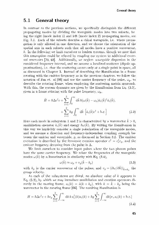
General theory
5.1 General theory
In contrast to the previous sections, we specifically distinguish the differentpropagating modes by dividing the waveguide modes into two subsets, be-ing the right (mode index 1) and left (mode index 2) propagating modes, seeFig. 5.1. Each of the subsets describe a chiral waveguide, i.e. where propa-gation is only allowed in one direction, and we choose the orientation of thespatial axis in each subsets such that all modes have a positive wavevector,𝑘. In the following we limit ourselves to lossless systems, though we note thatthis assumption could be relaxed by coupling our system to additional exter-nal reservoirs [70, 63]. Additionally, we neglect waveguide dispersion in theconsidered frequency interval, and we assume a localized scatterer (dipole ap-proximation), i.e. that the scattering occurs only at a single point in space, allas discussed in Chapter 3. Instead of describing the Hamiltonian in a framerotating with the emitter frequency as in the previous chapters, we follow thenotation of Fan et. al [66] and use the carrier frequency of the pulse, 𝜔p, todescribe the rotating frame, when employing the scattering matrix approach.With this, the system dynamics are given by the Hamiltonian from Eq. (3.3),given in a frame rotating with the pulse frequency, 𝜔p,
= ~∆𝑐†𝑐+
2∑𝑖=1
∫ ∞
0
d𝑘 ~(𝜔(𝑘) − 𝜔p)𝑖(𝑘)†𝑖(𝑘),
+
2∑𝑖=1
~𝑔∫ ∞
0
d𝑘[𝑖(𝑘)𝑐† + h.c.
](5.2)
Here each mode in subsystem 1 and 2 is characterized by a wavevector 𝑘 > 0,annihilation operator 𝑖(𝑘) and energy ~𝜔(𝑘). By writing the Hamiltonian inthis way we implicitly consider a single polarization of the waveguide modes,and we assume a direction and frequency-independent coupling strength be-tween the emitter and waveguide, 𝑔, as discussed in Section 3.2. The emitterexcitation is described by the fermionic creation operator 𝑐† = 𝑐†𝑒𝑐𝑔, and theemitter frequency detuning from the pulse is ∆.
We limit ourselves to consider input pulses where the two photon pulseshave the same carrier frequency. We relate the frequencies of the waveguidemodes 𝜔(𝑘) by a linearization in similarity with Eq. (3.4),
𝜔(𝑘) ≈ 𝜔𝑝 + 𝑣𝑔(𝑘 − 𝑘𝑝) (5.3)
with 𝑘𝑝 is the carrier wavevector of the pulses, and 𝑣𝑔 = (𝜕𝜔/𝜕𝑘)|=𝑘𝑝the
group velocity.As each of the subsystems are chiral, no absolute value of 𝑘 appears in
Eq. (5.3), by which we may introduce annihilation and creation operators di-rectly in the moving frame, 𝑎𝑖(𝑘) = (𝑘 + 𝑘𝑝), with 𝑘 = 𝑘 − 𝑘𝑝 being thewavevector in the rotating frame [66]. The resulting Hamiltonian is
𝐻 = ~∆𝑐†𝑐+ ~𝑣𝑔2∑
𝑖=1
∫ ∞
−∞d𝑘 𝑘 𝑎†𝑖 (𝑘)𝑎𝑖(𝑘) + ~𝑔
2∑𝑖=1
∫ ∞
−∞d𝑘[𝜎+𝑎𝑖(𝑘) + h.c.]
(5.4)
45
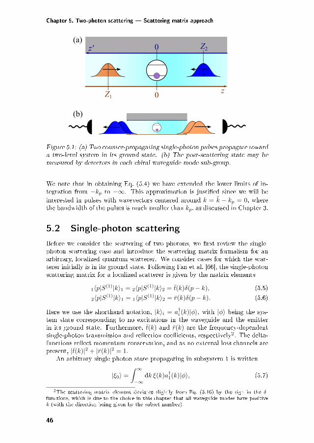
Chapter 5. Two-photon scattering — Scattering matrix approach
Z1 0
Z2
z
z' 0(a)
(b)
Figure 5.1: (a) Two counter-propagating single-photon pulses propagate towarda two-level system in its ground state. (b) The post-scattering state may bemeasured by detectors in each chiral waveguide mode sub-group.
We note that in obtaining Eq. (5.4) we have extended the lower limits of in-tegration from −𝑘𝑝 to −∞. This approximation is justified since we will beinterested in pulses with wavevectors centered around 𝑘 = 𝑘 − 𝑘𝑝 = 0, wherethe bandwidth of the pulses is much smaller than 𝑘𝑝, as discussed in Chapter 3.
5.2 Single-photon scattering
Before we consider the scattering of two photons, we first review the single-photon scattering case and introduce the scattering matrix formalism for anarbitrary, localized quantum scatterer. We consider cases for which the scat-terer initially is in its ground state. Following Fan et al. [66], the single-photonscattering matrix for a localized scatterer is given by the matrix elements
1⟨𝑝|𝑆(1)|𝑘⟩1 = 2⟨𝑝|𝑆(1)|𝑘⟩2 = 𝑡(𝑘)𝛿(𝑝− 𝑘), (5.5)
2⟨𝑝|𝑆(1)|𝑘⟩1 = 1⟨𝑝|𝑆(1)|𝑘⟩2 = 𝑟(𝑘)𝛿(𝑝− 𝑘). (5.6)
Here we use the shorthand notation, |𝑘⟩𝑖 = 𝑎†𝑖 (𝑘)|𝜑⟩, with |𝜑⟩ being the sys-tem state corresponding to no excitations in the waveguide and the emitterin its ground state. Furthermore, 𝑡(𝑘) and 𝑟(𝑘) are the frequency-dependentsingle-photon transmission and reflection coefficients, respectively2. The delta-functions reflect momentum conservation, and as no external loss channels arepresent, |𝑡(𝑘)|2 + |𝑟(𝑘)|2 = 1.
An arbitrary single photon state propagating in subsystem 1 is written
|𝜉0⟩ =
∫ ∞
−∞d𝑘 𝜉(𝑘)𝑎†1(𝑘)|𝜑⟩, (5.7)
2The scattering matrix element deviates slightly from Eq. (3.16) by the sign in the 𝛿-functions, which is due to the choice in this chapter that all waveguide modes have positive𝑘 (with the direction being given by the subset number).
46
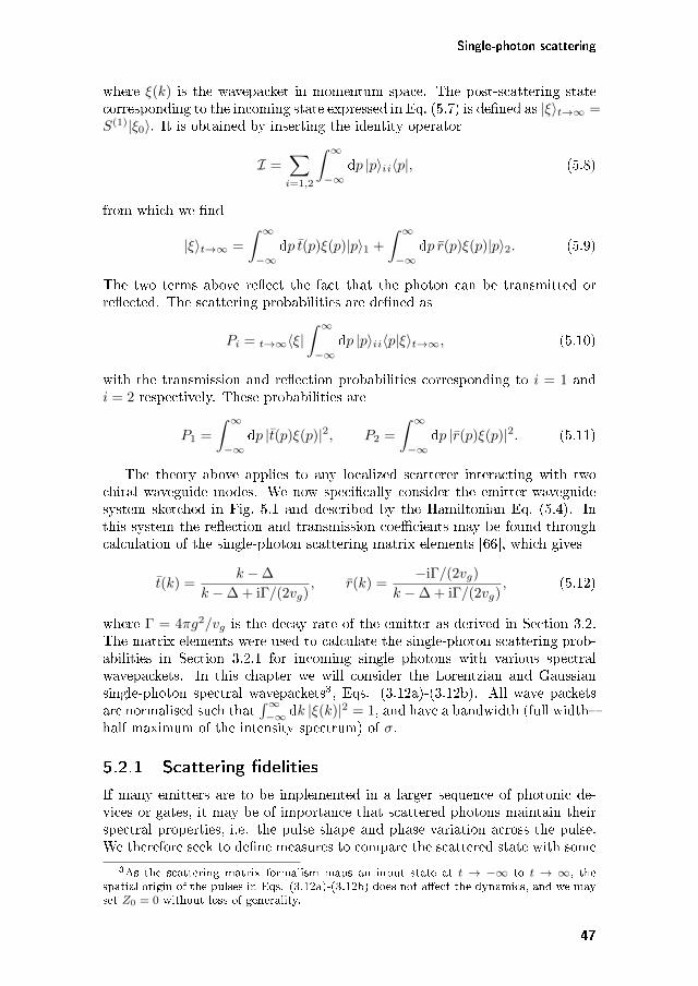
Single-photon scattering
where 𝜉(𝑘) is the wavepacket in momentum space. The post-scattering statecorresponding to the incoming state expressed in Eq. (5.7) is defined as |𝜉⟩𝑡→∞ =𝑆(1)|𝜉0⟩. It is obtained by inserting the identity operator
ℐ =∑𝑖=1,2
∫ ∞
−∞d𝑝 |𝑝⟩𝑖𝑖⟨𝑝|, (5.8)
from which we find
|𝜉⟩𝑡→∞ =
∫ ∞
−∞d𝑝 𝑡(𝑝)𝜉(𝑝)|𝑝⟩1 +
∫ ∞
−∞d𝑝 𝑟(𝑝)𝜉(𝑝)|𝑝⟩2. (5.9)
The two terms above reflect the fact that the photon can be transmitted orreflected. The scattering probabilities are defined as
𝑃𝑖 = 𝑡→∞⟨𝜉|∫ ∞
−∞d𝑝 |𝑝⟩𝑖𝑖⟨𝑝|𝜉⟩𝑡→∞, (5.10)
with the transmission and reflection probabilities corresponding to 𝑖 = 1 and𝑖 = 2 respectively. These probabilities are
𝑃1 =
∫ ∞
−∞d𝑝 |𝑡(𝑝)𝜉(𝑝)|2, 𝑃2 =
∫ ∞
−∞d𝑝 |𝑟(𝑝)𝜉(𝑝)|2. (5.11)
The theory above applies to any localized scatterer interacting with twochiral waveguide modes. We now specifically consider the emitter-waveguidesystem sketched in Fig. 5.1 and described by the Hamiltonian Eq. (5.4). Inthis system the reflection and transmission coefficients may be found throughcalculation of the single-photon scattering matrix elements [66], which gives
𝑡(𝑘) =𝑘 − ∆
𝑘 − ∆ + iΓ/(2𝑣𝑔), 𝑟(𝑘) =
−iΓ/(2𝑣𝑔)
𝑘 − ∆ + iΓ/(2𝑣𝑔), (5.12)
where Γ = 4𝜋𝑔2/𝑣𝑔 is the decay rate of the emitter as derived in Section 3.2.The matrix elements were used to calculate the single-photon scattering prob-abilities in Section 3.2.1 for incoming single photons with various spectralwavepackets. In this chapter we will consider the Lorentzian and Gaussiansingle-photon spectral wavepackets3, Eqs. (3.12a)-(3.12b). All wave packetsare normalised such that
∫∞−∞ d𝑘 |𝜉(𝑘)|2 = 1, and have a bandwidth (full width–
half maximum of the intensity spectrum) of 𝜎.
5.2.1 Scattering fidelities
If many emitters are to be implemented in a larger sequence of photonic de-vices or gates, it may be of importance that scattered photons maintain theirspectral properties, i.e. the pulse shape and phase variation across the pulse.We therefore seek to define measures to compare the scattered state with some
3As the scattering matrix formalism maps an input state at 𝑡 → −∞ to 𝑡 → ∞, thespatial origin of the pulses in Eqs. (3.12a)-(3.12b) does not affect the dynamics, and we mayset 𝑍0 = 0 without loss of generality.
47
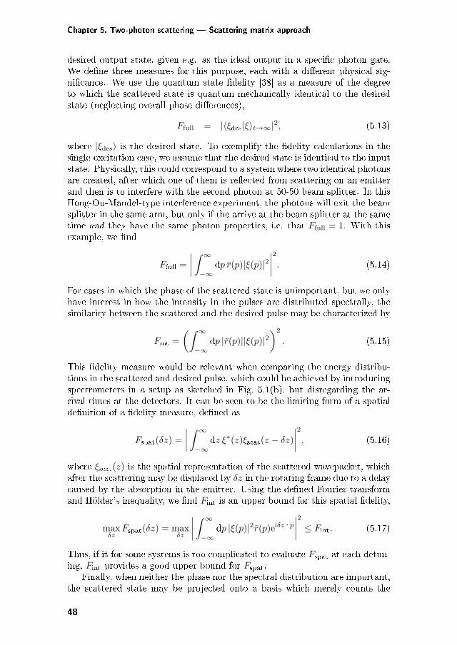
Chapter 5. Two-photon scattering — Scattering matrix approach
desired output state, given e.g. as the ideal output in a specific photon gate.We define three measures for this purpose, each with a different physical sig-nificance. We use the quantum state fidelity [38] as a measure of the degreeto which the scattered state is quantum mechanically identical to the desiredstate (neglecting overall phase differences),
𝐹full = |⟨𝜉des|𝜉⟩𝑡→∞|2, (5.13)
where |𝜉des⟩ is the desired state. To exemplify the fidelity calculations in thesingle-excitation case, we assume that the desired state is identical to the inputstate. Physically, this could correspond to a system where two identical photonsare created, after which one of them is reflected from scattering on an emitterand then is to interfere with the second photon at 50-50 beam splitter. In thisHong-Ou-Mandel-type interference experiment, the photons will exit the beamsplitter in the same arm, but only if the arrive at the beam splitter at the sametime and they have the same photon properties, i.e. that 𝐹full = 1. With thisexample, we find
𝐹full =
∫ ∞
−∞d𝑝 𝑟(𝑝)|𝜉(𝑝)|2
2. (5.14)
For cases in which the phase of the scattered state is unimportant, but we onlyhave interest in how the intensity in the pulses are distributed spectrally, thesimilarity between the scattered and the desired pulse may be characterized by
𝐹int =
(∫ ∞
−∞d𝑝 |𝑟(𝑝)||𝜉(𝑝)|2
)2
. (5.15)
This fidelity measure would be relevant when comparing the energy distribu-tions in the scattered and desired pulse, which could be achieved by introducingspectrometers in a setup as sketched in Fig. 5.1(b), but disregarding the ar-rival times at the detectors. It can be seen to be the limiting form of a spatialdefinition of a fidelity measure, defined as
𝐹spat(𝛿𝑧) =
∫ ∞
−∞d𝑧 𝜉*(𝑧)𝜉scat(𝑧 − 𝛿𝑧)
2, (5.16)
where 𝜉scat(𝑧) is the spatial representation of the scattered wavepacket, whichafter the scattering may be displaced by 𝛿𝑧 in the rotating frame due to a delaycaused by the absorption in the emitter. Using the defined Fourier transformand Hölder’s inequality, we find 𝐹int is an upper bound for this spatial fidelity,
max𝛿𝑧
𝐹spat(𝛿𝑧) = max𝛿𝑧
∫ ∞
−∞d𝑝 |𝜉(𝑝)|2𝑟(𝑝)ei𝛿𝑧 · 𝑝
2≤ 𝐹int. (5.17)
Thus, if it for some systems is too complicated to evaluate 𝐹spat at each detun-ing, 𝐹int provides a good upper bound for 𝐹spat.
Finally, when neither the phase nor the spectral distribution are important,the scattered state may be projected onto a basis which merely counts the
48
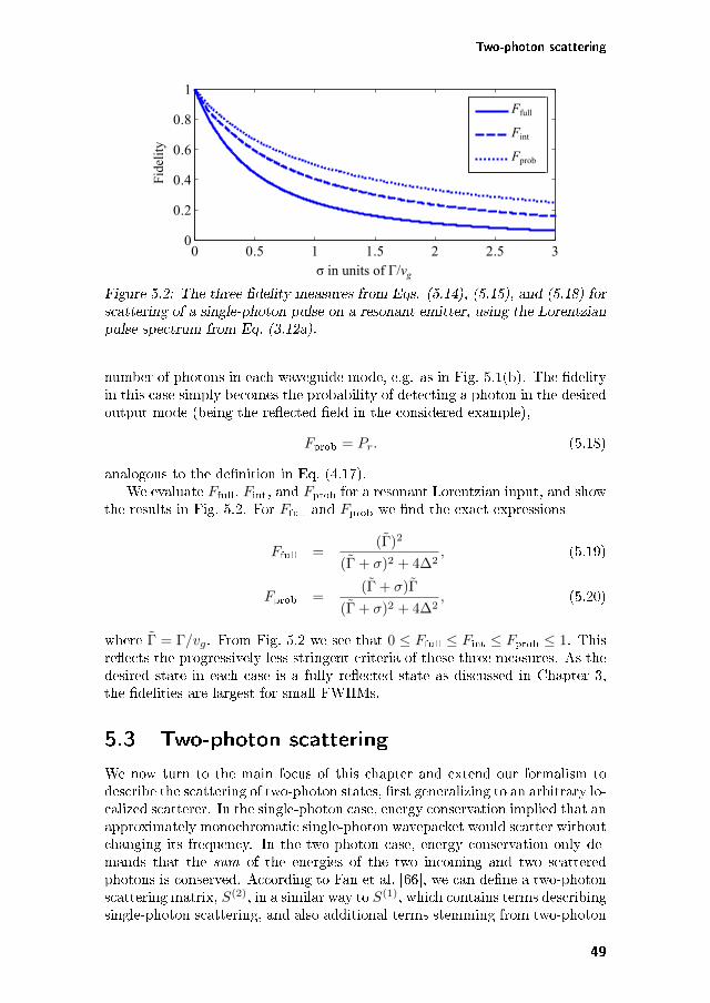
Two-photon scattering
0 0.5 1 1.5 2 2.5 30
0.2
0.4
0.6
0.8
1Ffull
Fint
FprobF
idel
ity
σ in units of Γ/vg
Figure 5.2: The three fidelity measures from Eqs. (5.14), (5.15), and (5.18) forscattering of a single-photon pulse on a resonant emitter, using the Lorentzianpulse spectrum from Eq. (3.12a).
number of photons in each waveguide mode, e.g. as in Fig. 5.1(b). The fidelityin this case simply becomes the probability of detecting a photon in the desiredoutput mode (being the reflected field in the considered example),
𝐹prob = 𝑃𝑟. (5.18)
analogous to the definition in Eq. (4.17).We evaluate 𝐹full, 𝐹int, and 𝐹prob for a resonant Lorentzian input, and show
the results in Fig. 5.2. For 𝐹full and 𝐹prob we find the exact expressions
𝐹full =(Γ)2
(Γ + 𝜎)2 + 4∆2, (5.19)
𝐹prob =(Γ + 𝜎)Γ
(Γ + 𝜎)2 + 4∆2, (5.20)
where Γ = Γ/𝑣𝑔. From Fig. 5.2 we see that 0 ≤ 𝐹full ≤ 𝐹int ≤ 𝐹prob ≤ 1. Thisreflects the progressively less stringent criteria of these three measures. As thedesired state in each case is a fully reflected state as discussed in Chapter 3,the fidelities are largest for small FWHMs.
5.3 Two-photon scattering
We now turn to the main focus of this chapter and extend our formalism todescribe the scattering of two-photon states, first generalizing to an arbitrary lo-calized scatterer. In the single-photon case, energy conservation implied that anapproximately monochromatic single-photon wavepacket would scatter withoutchanging its frequency. In the two-photon case, energy conservation only de-mands that the sum of the energies of the two incoming and two scatteredphotons is conserved. According to Fan et al. [66], we can define a two-photonscattering matrix, 𝑆(2), in a similar way to 𝑆(1), which contains terms describingsingle-photon scattering, and also additional terms stemming from two-photon
49
Chapter 5. Two-photon scattering — Scattering matrix approach
scattering processes. The additional terms involve four-wave mixing mecha-nisms between the two incoming and two scattered photons [66, 121].
In the rotating frame, a general two-photon state in the momentum repre-sentation is written as
|𝛽⟩ = 1√2
∫ ∞
−∞d𝑘∫ ∞
−∞d𝑘′ 𝛽11(𝑘, 𝑘′)𝑎†1(𝑘)𝑎†1(𝑘′)|𝜑⟩
+ 1√2
∫ ∞
−∞d𝑘∫ ∞
−∞d𝑘′ 𝛽22(𝑘, 𝑘′)𝑎†2(𝑘)𝑎†2(𝑘′)|𝜑⟩
+
∫ ∞
−∞d𝑘∫ ∞
−∞d𝑘′ 𝛽12(𝑘, 𝑘′)𝑎†1(𝑘)𝑎†2(𝑘′)|𝜑⟩, (5.21)
normalized such that∫∞−∞ d𝑘
∫∞−∞ d𝑘′ (|𝛽11(𝑘, 𝑘′)|2+|𝛽12(𝑘, 𝑘′)|2+|𝛽22(𝑘, 𝑘′)|2)
= 1. Introducing the notation |𝑘𝑘′⟩𝑖𝑖′ = 𝑖′𝑖⟨𝑘′𝑘|† = 𝑎†𝑖 (𝑘)𝑎†𝑖′(𝑘′)|𝜑⟩, the two-
photon scattering elements are [66]
𝑗𝑗′⟨𝑝𝑝′|𝑆(2)|𝑘𝑘′⟩𝑖𝑖′ = 𝛼𝑗𝑖,𝑘𝛼𝑗′𝑖′,𝑘′𝛿(𝑘 − 𝑝)𝛿(𝑘′ − 𝑝′)
+ 𝛼𝑗′𝑖,𝑘𝛼𝑗𝑖′,𝑘′𝛿(𝑘 − 𝑝′)𝛿(𝑘′ − 𝑝)
+ 14𝐵𝑝𝑝′𝑘𝑘′𝛿(𝑝+ 𝑝′ − 𝑘 − 𝑘′), (5.22)
for 𝑖, 𝑗 ∈ 1, 2, and where
𝛼𝑗𝑖,𝑘 =
𝑡(𝑘) if 𝑖 = 𝑗
𝑟(𝑘) if 𝑖 = 𝑗(5.23)
are the single photon reflection and transmission matrix elements. Here 𝐵𝑝𝑝′𝑘𝑘′
describes interactions between the two incoming and the two scattered photons,and is determined by the specific localized scatterer considered. As in the single-photon case, to find the scattered state, we insert the identity operator, whichis now given by
ℐ =
∫ ∞
−∞d𝑝∫ ∞
−∞d𝑝′[
1
2|𝑝′𝑝⟩1111⟨𝑝𝑝′| + |𝑝′𝑝⟩2112⟨𝑝𝑝′| +
1
2|𝑝′𝑝⟩2222⟨𝑝𝑝′|
].
(5.24)
In this chapter we specifically considering two incoming, counter-propagatingphotons. Thus 𝛽12 is the only non-zero expansion coefficient in Eq. (5.21),which results in the post-scattering state
|𝛽⟩𝑡→∞ =
∫ ∞
−∞d𝑝∫ ∞
−∞d𝑝′
1
2
[(𝑡(𝑝)𝑟(𝑝′) + 𝑟(𝑝)𝑡(𝑝′))𝛽12(𝑝, 𝑝′) + 1
4𝑏12(𝑝, 𝑝′)
]𝑎†1(𝑝)𝑎†1(𝑝′)
+
[(𝑟(𝑝)𝑟(𝑝′) + 𝑡(𝑝)𝑡(𝑝′))𝛽12(𝑝, 𝑝′) +
1
4𝑏12(𝑝, 𝑝′)
]𝑎†1(𝑝)𝑎†2(𝑝′)
+1
2
[(𝑡(𝑝)𝑟(𝑝′) + 𝑟(𝑝)𝑡(𝑝′))𝛽12(𝑝, 𝑝′) +
1
4𝑏12(𝑝, 𝑝′)
]𝑎†2(𝑝)𝑎†2(𝑝′)
|𝜑⟩.
(5.25)
50
Two-photon scattering
The first term in each of the three square brackets in Eq. (5.25) representssingle photon scattering processes, containing the appropriate combinations oftransmission and reflection coefficients connecting the initial and final photonconfigurations. I.e. to obtain the output state with photons in different modes,either both must be reflected, 𝑟(𝑝)𝑟(𝑝′), or both transmitted, 𝑡(𝑝)𝑡(𝑝′), givenin the third line of Eq. (5.25). Multi-photon process are contained in thepulse-dependent contribution 𝑏12(𝑝, 𝑝′), which describes processes induced bythe emitter non-linearity, and is given by
𝑏12(𝑝, 𝑝′) =
∫ ∞
−∞d𝑘 𝛽12(𝑘, 𝑝+ 𝑝′ − 𝑘)𝐵𝑝𝑝′𝑘(𝑝+𝑝′−𝑘). (5.26)
We define 𝑃11 (𝑃22) as the probability that both photons are measured propa-gating in waveguide mode 1 (mode 2), and 𝑃12 the probability that one photonpropagates in each waveguide mode. From Eq. (5.25) we find
𝑃11 =1
2
∫ ∞
−∞d𝑝∫ ∞
−∞d𝑝′(𝑡(𝑝)𝑟(𝑝′) + 𝑟(𝑝)𝑡(𝑝′))𝛽12(𝑝, 𝑝′) +
1
4𝑏12(𝑝, 𝑝′)
2,
(5.27)
𝑃12 =
∫ ∞
−∞d𝑝∫ ∞
−∞d𝑝′(𝑡(𝑝)𝑡(𝑝′) + 𝑟(𝑝)𝑟(𝑝′))𝛽12(𝑝, 𝑝′) +
1
4𝑏12(𝑝, 𝑝′)
2, (5.28)
with 𝑃11 = 𝑃22 and 𝑃11 + 𝑃12 + 𝑃22 = 1.As for the single photon case, we will be interested in comparing the scat-
tered two-photon state described by Eq. (5.25) to some desired state using thefidelity measures we have introduced in Eqs. (5.14), (5.15), and (5.18). InChapter 4 we demonstrated numerically how a two-level emitter may act as anon-linear beam splitter. Thus, it would of relevance to compare the scatteredto a scattered state obtained by replacing the emitter with a 50-50 beam split-ter, which preserves the shape and phase of the input photons. In this case thedesired state would be
|𝛽des⟩ =1√2
∫ ∞
−∞d𝑘∫ ∞
−∞d𝑘′ 𝛽12(𝑘, 𝑘′)
×[
1√2𝑎†1(𝑘)𝑎†1(𝑘′) +
1√2𝑎†2(𝑘)𝑎†2(𝑘′)
]|𝜑⟩. (5.29)
With this desired state our fidelity measures become
𝐹full =
∫ ∞
−∞d𝑝
∫ ∞
−∞d𝑝′𝛽*
12(𝑝, 𝑝′)𝛽′12(𝑝, 𝑝′)
2(5.30)
𝐹int =
[∫ ∞
−∞d𝑝
∫ ∞
−∞d𝑝′|𝛽12(𝑝, 𝑝′)| |𝛽′
12(𝑝, 𝑝′)|]2
(5.31)
𝐹prob = 𝑃11 + 𝑃22 (5.32)
with 𝛽′12(𝑝, 𝑝′) = (𝑡(𝑝)𝑟(𝑝′) + 𝑟(𝑝)𝑡(𝑝′))𝛽12(𝑝, 𝑝′) + 1
4𝑏12(𝑝, 𝑝′).
51
Chapter 5. Two-photon scattering — Scattering matrix approach
5.3.1 Two-level emitter
The theory presented above is valid for any localized scatterer. We now specif-ically consider the two-level-emitter–waveguide system described by Eq. (5.4),and focus here only on pulses starting equidistantly from the emitter. Further-more, we only treat pairs of input pulses with the same spectral linewidth, al-though the formalism can be straightforwardly extended to more general cases.For a two-level-emitter the single photon transmission and reflection matrixelements 𝑡(𝑘) and 𝑟(𝑘) are given by Eq. (5.12), while the two-photon scatteringelement is [66]
𝐵𝑝𝑝′𝑘𝑘′ = i
√Γ
𝜋𝑠(𝑝)𝑠(𝑝′)[𝑠(𝑘) + 𝑠(𝑘′)], (5.33)
where
𝑠(𝑘) =
√Γ/𝑣𝑔
𝑘 − ∆ + iΓ/(2𝑣𝑔). (5.34)
We only consider uncorrelated photon input states, and as such 𝛽(𝑘, 𝑘′) is asymmetrized product of two single-photon wavepackets 𝛽(𝑘, 𝑘′) = [𝜉(𝑘)𝜉′(𝑘′)+𝜉′(𝑘)𝜉(𝑘′)], which is normalized as
∫∞−∞ d𝑘
∫∞−∞ d𝑘′ |𝛽(𝑘, 𝑘′)|2 = 1.
We begin our analysis of the scattered state by considering correlations inphoton detection events in the two waveguide mode subsets, as depicted inFig. 5.1(b). In this case no information regarding the spectrum and phase ofthe scattered photons is obtained, and the appropriate fidelity measure is 𝐹prob,which is equal to 1 minus the probability of detecting a coincidence in the twodetectors, i.e. for 𝐹prob = 1 no coincidence events are measured (a perfectHong-Ou-Mandel dip would be observed). In Fig. 5.3(a), 𝐹prob is calculatedfor Gaussian and Lorentzian input pulses for zero detuning (∆ = 0), for whichthe interaction between the pulses and emitter is greatest. We see that veryhigh fidelities are obtained, reaching values of ∼ 80% for the Lorentzian inputand ∼ 90% for the Gaussian. This is equivalent to the result in Fig. 4.7,wheremaximal correlations are achieved in the regime where the emitter andpulse linewidth are similar. Interestingly, although the Lorentzian pulse shapeis well-known to be the optimal pulse shape for maximally exciting the two-levelemitter with a single photon [103], it is not the optimal shape for maximizingthe directional correlations in the scattered state.
The high fidelities obtained demonstrate that the scattered states are highlydirectionally entangled, in analogy with the effect of an optical beam-splitter.However, in contrast to the classical beam splitter, the high correlation seenhere is induced solely by non-linearities. To demonstrate that the high direc-tional correlations indeed stem from non-linearities, in Fig. 5.3(a) we also showthe case where the non-linear two-photon interaction term 𝑏12(𝑝, 𝑝′) has beenartificially set to 0 (dashed curves). For an uncorrelated two-photon input pulsewhich is resonant with the emitter and which has a symmetric spectral wave-function amplitude, |𝜉(−𝑘)|2 = |𝜉(𝑘)|2, as is the case here, Eq. (5.27) reduces
52
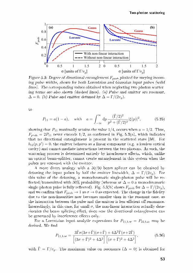
Two-photon scattering
0
0.2
0.4
0.6
0.8
1
Fpr
ob
σ [units of Γ/vg]0 0.5 1 1.5 2
With non-linear interactionWithout non-linear interaction
Gauss
LorentzLorentz
(a) (b)
σ [units of Γ/vg]0 0.5 1 1.5 2
Gauss
Figure 5.3: Degree of directional entanglement 𝐹prob plotted for varying incom-ing pulse widths, shown for both Lorentzian and Gaussian input pulses (solidlines). The corresponding values obtained when neglecting two-photon scatter-ing terms are also shown (dashed lines). (a) Pulse and emitter are resonant,∆ = 0. (b) Pulse and emitter detuned by ∆ = Γ/(2𝑣𝑔).
to
𝑃11 = 𝑎(1 − 𝑎), with 𝑎 =
∫ ∞
−∞d𝑝
(Γ/2)2
𝑝2 + (Γ/2)2|𝜉(𝑝)|2, (5.35)
showing that 𝑃11 maximally attains the value 1/4, occurs when 𝑎 = 1/2. Thus,𝐹prob = 2𝑃11 never exceeds 1/2, as confirmed in Fig. 5.3(a), which indicatesthat no directional entanglement is present in the scattered state [38]. For𝑏12(𝑝, 𝑝′) = 0, the emitter behaves as a linear component (e.g. a lossless opticalcavity) and cannot mediate interactions between the two photons. As such, thescattering process is determined entirely by interference effects, which, unlikean optical beam-splitter, cannot create entanglement in this system when thepulses are resonant with the emitter.
A more direct analogy with a 50/50 beam splitter can be obtained bydetuning the input pulses by half the emitter linewidth, ∆ = Γ/(2𝑣𝑔). Forthis value of the detuning, a monochromatic single-photon pulse will be re-flected/transmitted with 50% probability (whereas at ∆ = 0 a monochromaticsingle-photon pulse is fully reflected). Fig. 5.3(b) shows 𝐹prob for ∆ = Γ/(2𝑣𝑔),and we confirm that 𝐹prob → 1 as 𝜎 → 0 as expected. The change in the fidelitydue to the non-linearities now becomes smaller than in the resonant case, asthe interaction between the pulse and the emitter is less efficient off resonance.Interestingly, in this case, for small 𝜎, the non-linear interaction actually dete-riorates the beam splitting effect, since now the directional entanglement canbe generated by interference effects only.
For a Lorentzian input analytic expressions for 𝑃11,Lor = 𝑃22,Lor may bederived. We find
𝑃11,Lor =3Γ𝜎(3𝜎+Γ)(𝜎+Γ) + 4∆2Γ(𝜎+2Γ)[(3𝜎 + Γ)2 + 4∆2
] [(𝜎 + Γ)2 + 4∆2
] , (5.36)
with Γ = Γ/𝑣𝑔. The maximum value on resonance (∆ = 0) is obtained for
53
Chapter 5. Two-photon scattering — Scattering matrix approach
𝜎/Γ = 3−1/2 ≈ 0.57, at which point 𝑃11,Lor ≈ 0.40 (and 𝐹prob = 2𝑃11,Lor ≈0.8), in agreement with Fig. 5.3(a). In comparison, with no non-linear terms,𝑏12(𝑝, 𝑝′) = 0, the scattering probability becomes
𝑃 one11,Lor =
𝜎Γ(𝜎 + Γ)2 + 4∆2Γ(𝜎 + 2Γ)[(𝜎 + Γ)2 + 4∆2
]2 , (5.37)
which has an on-resonance maximum for 𝜎 = Γ, giving 𝐹prob = 2𝑃 one𝑅𝑅,Lor =
1/2. Thus, for the Lorentzian pulse, non-linearities increase the scatteringprobability by a factor of 𝑃11,Lor/𝑃
one11,Lor = 1 + 2/(1 + 3𝜎/Γ) on resonance.
For 𝜎 → ∞, the interaction with the emitter becomes infinitely weak and noenhancement is present. In the opposite limit of 𝜎 → 0, the enhancement factoris 3.
5.3.2 Scattering fidelities
As discussed above, if the scatterer is to be implemented in a larger opticalcircuit, in addition to considering in which direction the photons scatter, theamplitude and phase of the different frequency components may also be im-portant. In such a case, 𝐹prob is no longer a sufficient fidelity measure, sinceit contains only directional information. As illustrated in Fig. 5.4, where weplot the intensity spectrum of a scattered Gaussian wavepacket, the spectraof the scattered pulses change significantly during the scattering process. Forinput pulses with a narrow spectral linewidth compared to the emitter (1strow), the pulse power at the emitter position remains low due to the corre-sponding broad spatial profiles of the pulses. In that case, the non-linearity isonly weakly addressed, and the individual photons are predominately reflected.A weak non-linearity-induced four-wave mixing process is signified by the ap-pearance of diagonal features, as one photon achieves a larger energy, while theenergy of the other decreases. When the pulse and emitter linewidths are com-parable (2nd row), the predicted strong directional correlation is induced [121],with the pulse profile being almost preserved. For spectrally broad pulses (3rdrow), only the near-resonant part of the spectrum interacts with the emitter.We see that the spectral components at the emitter frequency are absent fromthe transmitted pulse since these have been reflected without significant two-photon effects.
Interestingly, the fact that the pulse spectrum is almost perfectly preservedwhen the pulse and emitter linewidths are comparable (2nd row) can be at-tributed to non-linearities. This can be seen in the 4th row, where we againshow the initial and scattered spectra for the case 𝜎 = Γ, but where we haveartificially set the non-linear term equal to zero, 𝑏12 = 0. By comparison withthe 2nd row, we can clearly see that the non-linearities not only give rise to thedirectional entanglement, but also suppress changes to the spectral shape.
To quantify both the spectral and phase deviations between the scatteredand the desired state, all three fidelities defined in Eqs. (5.30)-(5.32) are shownin Fig. 5.5. By comparing 𝐹prob to 𝐹int, i.e. taking into account the differencein the spectra of the scattered and desired pulse (but not the phase), we see
54
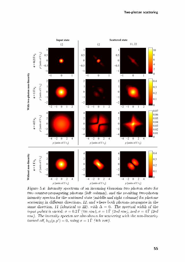
Two-photon scattering
p [units of Γ/vg]
p' [
unit
s of
Γ/vg]
p' [
unit
s of
Γ/vg]
p' [
unit
s of
Γ/vg]
12 11, 22
−2 −1 0 1 2
−2
−1
0
1
2
−2 −1 0 1 2
−2
−1
0
1
2
−2 −1 0 1 2
−2
−1
0
1
2
−1 0 1
−1
−0.5
0
0.5
1
−1 0 1
−1
−0.5
0
0.5
1
−1 0 1
−1
−0.5
0
0.5
1
0
2
4
6
8
10
−4 −2 0 2 4
−4
−2
0
2
4
−4 −2 0 2 4
−4
−2
0
2
4
−4 −2 0 2 4
−4
−2
0
2
4
0.010.020.030.040.050.060.07
Input state Scattered state
12
p [units of Γ/vg] p [units of Γ/vg]
0.1
0.2
0.3
0.4
0
0
p [units of Γ/vg]
−4 −2 0 2 4
−4
−2
0
2
4
−4 −2 0 2 4
−4
−2
0
2
4
−4 −2 0 2 4
−4
−2
0
2
4
p [units of Γ/vg] p [units of Γ/vg]
p' [
unit
s of
Γ/vg]
0.1
0.2
0.3
0.4
0
Wit
h t
wo-
ph
oton
non
-lin
eari
tyW
ith
out
non
-lin
eari
ty
σ =
4 Γ
/vg
σ =
1 Γ
/vg
σ =
1 Γ
/vg
σ =
0.2
Γ/vg
Figure 5.4: Intensity spectrum of an incoming Gaussian two-photon state fortwo counter-propagating photons (left column), and the resulting two-photonintensity spectra for the scattered state (middle and right columns) for photonsscattering in different directions, 12, and where both photons propagate in thesame direction, 11 (identical to 22), with ∆ = 0. The spectral width of theinput pulses is varied: 𝜎 = 0.2 Γ (1st row), 𝜎 = 1 Γ (2nd row), and 𝜎 = 4 Γ (3rdrow). The intensity spectra are also shown for scattering with the non-linearityturned off, 𝑏12(𝑝, 𝑝′) = 0, using 𝜎 = 1 Γ (4th row).
55
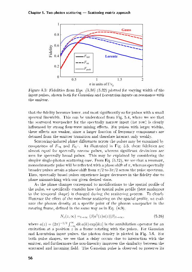
Chapter 5. Two-photon scattering — Scattering matrix approach
Gauss
LorentzFfull
Fint
Fprob
0
0.2
0.4
0.6
0.8
1
0.5 1 1.5 2σ in units of Γ/vg
Fid
elit
y
Figure 5.5: Fidelities from Eqs. (5.30)-(5.32) plotted for varying width of theinput pulses, shown both for Gaussian and Lorentzian inputs on resonance withthe emitter.
that the fidelity becomes lower, and most significantly so for pulses with a smallspectral linewidth. This can be understood from Fig. 5.4, where we see thatthe scattered wavepacket for the spectrally narrow input (1st row) is clearlyinfluenced by strong four-wave mixing effects. For pulses with larger widths,these effects are weaker, since a larger fraction of frequency components aredetuned from the emitter transition and therefore interact only weakly.
Scattering-induced phase differences across the pulses may be examined bycomparison of 𝐹int and 𝐹full. As illustrated in Fig. 5.5, these fidelities arealmost equal for spectrally narrow pulses, whereas significant deviations areseen for spectrally broad pulses. This may be explained by considering thesimpler single-photon scattering case. From Eq. (5.12), we see that a resonant,monochromatic pulse will be reflected with a phase shift of 𝜋, whereas spectrallybroader pulses attain a phase shift from 𝜋/2 to 3𝜋/2 across the pulse spectrum.Thus, spectrally broad pulses experience larger decreases in the fidelity due tophase mismatching with our given desired state.
As the phase changes correspond to modifications to the spatial profile ofthe pulse, we specifically consider how the spatial pulse profile (here analogousto the temporal shape) is changed during the scattering process. To clearlyillustrate the effect of the non-linear scattering on the spatial profile, we eval-uate the photon density at a specific point of the photon wavepacket in therotating frame, defined in the same way as in Eq. (4.9),
𝑁𝑧(𝑧,∞) =𝑡→∞ ⟨𝛽|𝑎†(𝑧)𝑎(𝑧)|𝛽⟩𝑡→∞, (5.38)
where 𝑎(𝑧) = (2𝜋)−1/2∫∞−∞ d𝑘 𝑎(𝑘) exp[i𝑘𝑧] is the annihilation operator for an
excitation at a position 𝑧 in a frame rotating with the pulses. For Gaussianand Lorentzian input pulses, the photon density is plotted in Fig. 5.6. Forboth pulse shapes, we see that a delay occurs due to interaction with theemitter, and furthermore the non-linearity improves the similarity between thescattered and incoming field. The Gaussian pulse is observed to preserve its
56
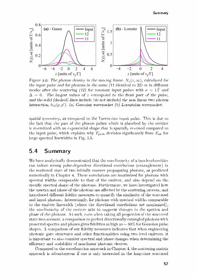
Summary
−6 −4 −2 0 2 4 60
0.2
0.4
0.6
0.8Input1211
−4 −2 0 2 40
0.5
1
1.5Input1211
z [units of vg/Γ] z [units of vg/Γ]
(a) - Gauss (b) - Lorentz
Nz(
z,
) [u
nits
of Γ
/vg]
8
Nz(
z,
) [u
nits
of Γ
/vg]
8
Figure 5.6: The photon density in the moving frame, 𝑁𝑧(𝑧,∞), calculated forthe input pulse and for photons in the same (11 identical to 22) or in differentmodes after the scattering (12) for resonant input pulses with 𝜎 = 1 Γ and∆ = 0. The largest values of 𝑧 correspond to the front part of the pulse,and the solid (dashed) lines include (do not include) the non-linear two-photoninteraction, 𝑏12(𝑝, 𝑝′). (a) Gaussian wavepacket (b) Lorentzian wavepacket.
spatial symmetry, as compared to the Lorentzian input pulse. This is due tothe fact that the part of the photon pulses which is absorbed by the emitteris re-emitted with an exponential shape that is spatially reversed compared tothe input pulse, which explains why 𝐹prob deviates significantly from 𝐹int forlarge spectral linewidths in Fig. 5.5.
5.4 Summary
We have analytically demonstrated that the non-linearity of a two-level-emittercan induce strong pulse-dependent directional correlations (entanglement) inthe scattered state of two initially counter propagating photons, as predictednumerically in Chapter 4. These correlations are maximized for photons withspectral widths comparable to that of the emitter, and also depend on thespecific spectral shape of the photons. Furthermore, we have investigated howthe spectra and phase of the photons are affected by the scattering process, andintroduced different fidelity measures to quantify the similarity of the scatteredand input photons. Interestingly, for photons with spectral widths comparableto the emitter linewidth (where the directional correlations are maximized),the non-linearity of the emitter acts to suppress changes in the spectra andphase of the photons. As such, even when taking all properties of the scatteredstate into account, a comparison to perfect directionally entangled photons withpreserved spectra and phases gives fidelities as high as∼ 80% for Gaussian pulseshapes. A comparison of our fidelity measures indicates that when engineeringphotonic gate structures and other functionalities using two-level-emitters, itis important to also consider spectral and phase changes when determining theefficiency and scalability of non-linear photonic devices.
Compared to the wavefunction approach in Chapter 4, the scattering matrixapproach is advantageous if one is only interested in the long-time scattered
57
Chapter 5. Two-photon scattering — Scattering matrix approach
state. This may be calculated computationally faster than in the wavefunctionapproach, whereas it necessitates a derivation of scatterer-specific one- and two-photon scattering matrix elements. This becomes complex for multi-componentscatterers or spatially separated scatterers, as compared to the wavefunctionapproach. Thus, the method to analysing two-photon scattering on a non-linearity should be chosen depending on the specific problem and the desiredinformation about the scattering process.
58
Chapter 6
Controlled phase gate
In this chapter we discuss how the results and understanding of non-linear two-photon scattering from the previous chapters may be employed in proposals fortwo-photon conditional gates and switches, where the presence of one photoninfluences the scattering of the second photon. Conditional two-qubit gatessuch as the CNOT gate or the controlled-phase (c-phase) gate are a funda-mental building block in the universal set of gates operations required in thestandard picture of quantum computing [3].
Using only beam splitters, phase shifters, and photon detectors, T. Ralphproposed in 2002 a scheme for a CNOT gate [122], where the non-linearitieswere obtained by projective measurements on ancilla arms. Due to its prob-abilistic nature, the succes probability of the gate is 1/9, where a success isindicated by a specific measurement outcome in the ancilla arms. The gatehas been experimentally implemented using free-space optics [16], and has alsorecently been implemented in an all-optical semiconductor platform using di-rectional couplers and quantum dots in micropillars as single-photon sources[123]. A disadvantage with the gate is its probabilistic nature, as the lowsuccess rate have major influence is several subsequent gates are to be em-ployed. One method to enhance the performance of these probabilistic gate isby quantum teleportation [15], which however relies on using multiple ancillawaveguides and photon detectors. As this quickly results in large structures forimplementation, current research focusses on implementation the conditionalgate operations in a deterministic setup instead.
Several recent experimental results demonstrate the possibility of creatingdeterministic controlled phase gates and photonic switches between the polar-isation state of a single photon and the spin state of an emitter. It has bothbeen demonstrated experimentally for Rubidium atoms coupled strongly to op-tical cavities [40, 124, 39] and recently also for a quantum dot inside a photoniccrystal cavity [42]. By applying single-qubit rotations to the atom mediatedby 𝜋/2-pulses from external lasers, the atom–cavity systems may work as con-ditional gates for qubit state encoded in the polarisation of two temporallyseparated photons. This was originally proposed by Duan and Kimble [125],and has been applied to a variety of systems, including also proposals with NV
59
Chapter 6. Controlled phase gate
centers [126].Deterministic switching operations between two photons may also be re-
alized using other encodings than in the polarisation degree of freedom. Foran emitter strongly coupled to an optical cavity, the atom dresses the energylevels of the cavity, given rise to energy levels of the dressed cavity which arenot equally spaced [24]. By using different frequencies of the control and thesignal photons, the frequencies may be chosen such that the signal only maycouple to the cavity if the control photon is present [44, 127, 128].
A different proposal by R. Johne et al. [129] describes a scheme for acontrolled-phase gate for two indistinguishable, temporally separated photons.Here the control photon is captured as an excitation of a QD inside an opticalcavity by electrically detuning the emitter out of resonance with the cavity.The emitter is detuned such that the energy for exciting the bi-exciton state ofthe QD exactly matches the energy of the incoming signal photon. Thus, thesignal photon can only couple to the emitter if the control photon was presentto excite the QD - giving the conditional operation. An advantage of using thisscheme is that the non-linearity-induced distortions in the photon spectra asdiscussed in the previous chapters do not occur [130], as the photons do notscatter at the same time. We will look further into this type of gate in the nextchapter.
In this chapter we propose an experimental setup for a deterministic control-led-phase gate for two uncorrelated, indistinguishable photons in the dual-railrepresentation, which employs two two-level emitters as non-linear components.The gate works best for input pulses with spectral linewidths comparable to thelinewidth of the emitter, which is also where the largest non-linear interaction isexpected, cf. the previous chapters. In this regime, the presence of one photonprevent the second photon from scattering on the emitter - in analogy with theeffect discussed above for the strongly coupled emitter–cavity systems.
In contrast to the deterministic gates discussed above, our proposal does notrely on any external modulations such as lasers to prepare or alter the emitterstate, and it does not need any dynamical trapping processes, which may be alarge benefit when discussing implementations. We demonstrate a gate fidelityof almost 80 %, which primarily limited by the non-linearity-induced spectralchanges.
In Section 6.1 the requirements for a controlled-phase gate is discussed,and we introduce the individual gate components. In Section 6.2 we introduceour gate proposal and evaluate the performance using the scattering matrixformalism introduced in Chapter 5. The results presented in this chapter arefrom an ongoing research collaboration with Mikkel Heuck and Prof. DirkEnglund from the Quantum Photonics Group at Massachusetts Institute ofTechnology.
6.1 The controlled phase gate
In a controlled phase (c-phase) gate, the state of a control qubit determineswhether a signal qubit attains a phase shift of 𝜋 or not [38]. Denoting the qubit
60
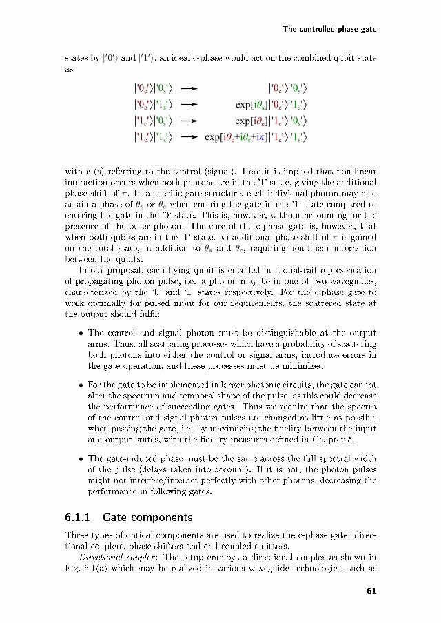
The controlled phase gate
states by |′0′⟩ and |′1′⟩, an ideal c-phase would act on the combined qubit stateas
exp[iθc]
exp[iθs]
exp[iθc+iθs+iπ]
'0c' '0s'
'0s''1c'
'0c' '1s'
'1c' '1s'
'0c' '0s'
'0s''1c'
'0c' '1s'
'1c' '1s'
with c (s) referring to the control (signal). Here it is implied that non-linearinteraction occurs when both photons are in the ’1’ state, giving the additionalphase shift of 𝜋. In a specific gate structure, each individual photon may alsoattain a phase of 𝜃𝑠 or 𝜃𝑐 when entering the gate in the ’1’ state compared toentering the gate in the ’0’ state. This is, however, without accounting for thepresence of the other photon. The core of the c-phase gate is, however, thatwhen both qubits are in the ’1’ state, an additional phase shift of 𝜋 is gainedon the total state, in addition to 𝜃𝑠 and 𝜃𝑐, requiring non-linear interactionbetween the qubits.
In our proposal, each flying qubit is encoded in a dual-rail representationof propagating photon pulse, i.e. a photon may be in one of two waveguides,characterized by the ’0’ and ’1’ states respectively. For the c-phase gate towork optimally for pulsed input for our requirements, the scattered state atthe output should fulfil:
∙ The control and signal photon must be distinguishable at the outputarms. Thus, all scattering processes which have a probability of scatteringboth photons into either the control or signal arms, introduce errors inthe gate operation, and these processes must be minimized.
∙ For the gate to be implemented in larger photonic circuits, the gate cannotalter the spectrum and temporal shape of the pulse, as this could decreasethe performance of succeeding gates. Thus we require that the spectraof the control and signal photon pulses are changed as little as possiblewhen passing the gate, i.e. by maximizing the fidelity between the inputand output states, with the fidelity measures defined in Chapter 5.
∙ The gate-induced phase must be the same across the full spectral widthof the pulse (delays taken into account). If it is not, the photon pulsesmight not interfere/interact perfectly with other photons, decreasing theperformance in following gates.
6.1.1 Gate components
Three types of optical components are used to realize the c-phase gate: direc-tional couplers, phase shifters and end-coupled emitters.
Directional coupler : The setup employs a directional coupler as shown inFig. 6.1(a) which may be realized in various waveguide technologies, such as
61
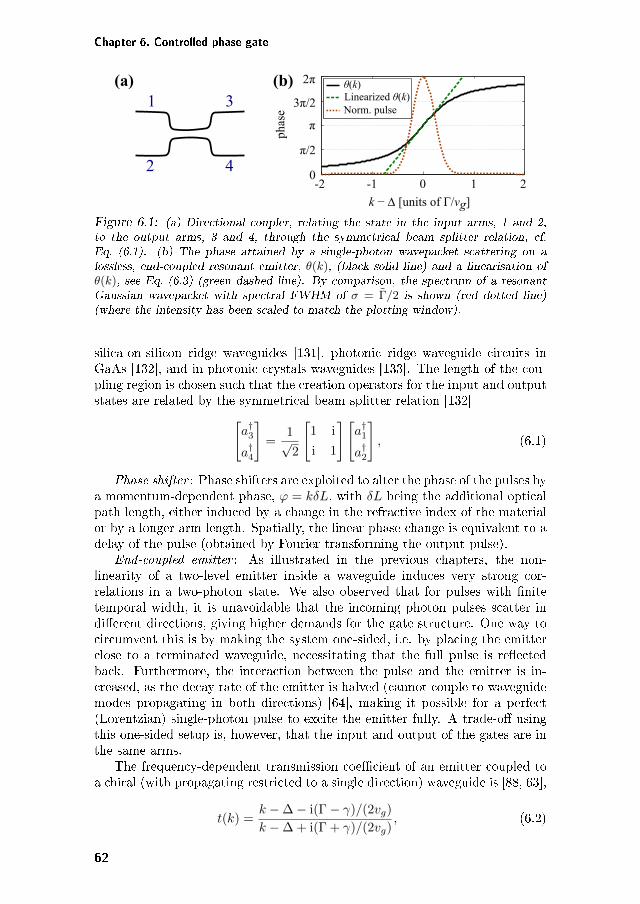
Chapter 6. Controlled phase gate
1
2
3
4
k − ∆ [units of Γ/vg]
π
2π
3π/2
π/2
0-1-2 0 1 2
phas
e
θ(k)
Norm. pulseLinearized θ(k)
(a) (b)
Figure 6.1: (a) Directional coupler, relating the state in the input arms, 1 and 2,to the output arms, 3 and 4, through the symmetrical beam splitter relation, cf.Eq. (6.1). (b) The phase attained by a single-photon wavepacket scattering on alossless, end-coupled resonant emitter, 𝜃(𝑘), (black solid line) and a linearisation of𝜃(𝑘), see Eq. (6.3) (green dashed line). By comparison, the spectrum of a resonantGaussian wavepacket with spectral FWHM of 𝜎 = Γ/2 is shown (red dotted line)(where the intensity has been scaled to match the plotting window).
silica-on-silicon ridge waveguides [131], photonic ridge waveguide circuits inGaAs [132], and in photonic crystals waveguides [133]. The length of the cou-pling region is chosen such that the creation operators for the input and outputstates are related by the symmetrical beam splitter relation [132][
𝑎†3
𝑎†4
]=
1√2
[1 i
i 1
][𝑎†1
𝑎†2
], (6.1)
Phase shifter : Phase shifters are exploited to alter the phase of the pulses bya momentum-dependent phase, 𝜙 = 𝑘𝛿𝐿, with 𝛿𝐿 being the additional opticalpath length, either induced by a change in the refractive index of the materialor by a longer arm length. Spatially, the linear phase change is equivalent to adelay of the pulse (obtained by Fourier-transforming the output pulse).
End-coupled emitter : As illustrated in the previous chapters, the non-linearity of a two-level emitter inside a waveguide induces very strong cor-relations in a two-photon state. We also observed that for pulses with finitetemporal width, it is unavoidable that the incoming photon pulses scatter indifferent directions, giving higher demands for the gate structure. One way tocircumvent this is by making the system one-sided, i.e. by placing the emitterclose to a terminated waveguide, necessitating that the full pulse is reflectedback. Furthermore, the interaction between the pulse and the emitter is in-creased, as the decay rate of the emitter is halved (cannot couple to waveguidemodes propagating in both directions) [64], making it possible for a perfect(Lorentzian) single-photon pulse to excite the emitter fully. A trade-off usingthis one-sided setup is, however, that the input and output of the gates are inthe same arms.
The frequency-dependent transmission coefficient of an emitter coupled toa chiral (with propagating restricted to a single direction) waveguide is [88, 63],
𝑡(𝑘) =𝑘 − ∆ − i(Γ − 𝛾)/(2𝑣𝑔)
𝑘 − ∆ + i(Γ + 𝛾)/(2𝑣𝑔), (6.2)
62
Gate setup
with 𝑘 being the momentum in a frame rotating with the carrier frequencyof the pulse. The momentum detuning of the emitter from the pulse is ∆,and Γ denotes the emitter decay rate (which is halved compared to the decayrate defined in Chapter 3). Emitter losses are introduced by the substitution∆ → ∆ − i𝛾/(2𝑣𝑔) in the single-photon scattering elements, with 𝛾 being theloss rate of the emitter into other modes than the waveguide modes [63].
Some insight may be gained about the scattering-induced phase by con-sidering the loss-less case. For 𝛾 = 0, |𝑡(𝑘)| = 1, and thus 𝑡(𝑘) may also bedescribed by a complex phase, 𝑡(𝑘) = ei𝜃(𝑘), such that an incoming single-photon pulse with a spectral wavepacket 𝜉(𝑘) results in a scattered wavepacketof 𝜉scat(𝑘) = ei𝜃(𝑘)𝜉(𝑘). This phase is shown in Fig. 6.1 in the case 𝛾 = 0.If the incoming single-photon pulse has a carrier frequency corresponding tothe emitter transition, ∆ = 0, and if the pulse has a sufficiently narrow spec-trum compared to the linewidth of the emitter, 𝜃(𝑘) may be approximated bya Taylor expansion,
𝑡(𝑘) = exp[i𝜋 + i4𝑘/Γ +𝑂(𝑘3)
], (6.3)
with 𝑂(𝑘3) containing terms of third order or higher in 𝑘. Pulses with a narrowspectral width compared to the emitter linewidth will, apart from a constantphase shift of 𝜋, gain a phase of 4𝑘/Γ, which in time is exactly equivalent toa temporal delay of ∆𝑡 = 4/Γ. This delay is caused by the interactions withthe emitter due to absorption and re-emission. For spectrally broader pulses,higher order terms in 𝑘 do have an influence and introduces different chirpingeffects, as seen from Eq. (6.3) and the discussion in Chapter 3.
6.2 Gate setup
Our proposal for a c-phase gate is illustrated in Fig. 6.2, which works for twouncorrelated single-photon pulses with the same spectral wavefuntion, wherethe control and single photon are represented in a dual-rail basis. The ’1’ arms(inner arms) are connected by a 50-50 directional coupler, and at each outputport of the coupler is an end-coupled two-level emitter. The coupler creates asuperposition state of two photon being either in the upper or lower arm on theright side of the beam splitter. Thus, when the photon state scatters on theemitters, it only contains component with two photons, and thus the full stateis affected by the non-linearity. In this way, the non-linearity may be exploitedthe most. The outer arms (’0’ arms) contain a phase shifter to compensate fordelays in the ’1’ arms, as predicted by Eq. (6.3). Note, that due to the choiceof directional coupler, the output port of the ’1’ control and signal states areflipped, as indicated in Fig. 6.2. A similar setup is discussed in [96, 134], buthere with the purpose of using it as photon sorter, quantum non-demolitiondetector, and Bell-state analyzer.
As the gate proposal is one-sided, meaning that the input and output armsof the gate are the same, the whole setup may be "unfolded" to a chiral scheme(where the waveguides only allow propagation in one direction), if the overallphase due to the reflection is omitted. An important requirement is, however,
63
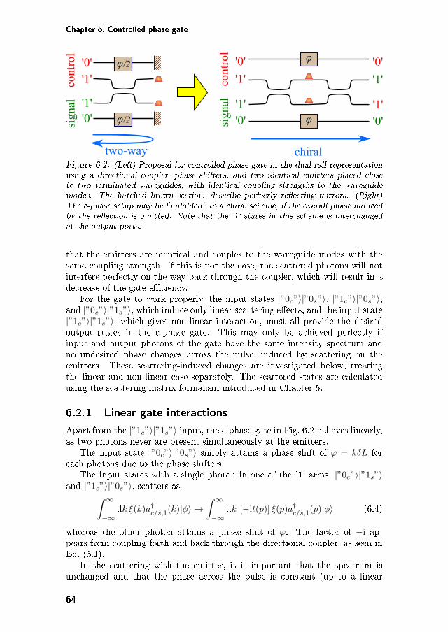
Chapter 6. Controlled phase gate
control
φ/2
φ/2'0''1'
signal
'0''1'
φ
φ
control
'0'
'1'
signal
'0''1'
'0'
'1'
'0''1'
chiraltwo-wayFigure 6.2: (Left) Proposal for controlled phase gate in the dual rail representationusing a directional coupler, phase shifters, and two identical emitters placed closeto two terminated waveguides, with identical coupling strengths to the waveguidemodes. The hatched brown sections describe perfectly reflecting mirrors. (Right)The c-phase setup may be "unfolded" to a chiral scheme, if the overall phase inducedby the reflection is omitted. Note that the ’1’ states in this scheme is interchangedat the output ports.
that the emitters are identical and couples to the waveguide modes with thesame coupling strength. If this is not the case, the scattered photons will notinterfere perfectly on the way back through the coupler, which will result in adecrease of the gate efficiency.
For the gate to work properly, the input states |”0𝑐”⟩|”0𝑠”⟩, |”1𝑐”⟩|”0𝑠”⟩,and |”0𝑐”⟩|”1𝑠”⟩, which induce only linear scattering effects, and the input state|”1𝑐”⟩|”1𝑠”⟩, which gives non-linear interaction, must all provide the desiredoutput states in the c-phase gate. This may only be achieved perfectly ifinput and output photons of the gate have the same intensity spectrum andno undesired phase changes across the pulse, induced by scattering on theemitters. These scattering-induced changes are investigated below, treatingthe linear and non-linear case separately. The scattered states are calculatedusing the scattering matrix formalism introduced in Chapter 5.
6.2.1 Linear gate interactions
Apart from the |”1𝑐”⟩|”1𝑠”⟩ input, the c-phase gate in Fig. 6.2 behaves linearly,as two photons never are present simultaneously at the emitters.
The input state |”0𝑐”⟩|”0𝑠”⟩ simply attains a phase shift of 𝜙 = 𝑘𝛿𝐿 foreach photons due to the phase shifters.
The input states with a single photon in one of the ’1’ arms, |”0𝑐”⟩|”1𝑠”⟩and |”1𝑐”⟩|”0𝑠”⟩, scatters as∫ ∞
−∞d𝑘 𝜉(𝑘)𝑎†𝑐/𝑠,1(𝑘)|𝜑⟩ →
∫ ∞
−∞d𝑘 [−i𝑡(𝑝)] 𝜉(𝑝)𝑎†𝑐/𝑠,1(𝑝)|𝜑⟩ (6.4)
whereas the other photon attains a phase shift of 𝜙. The factor of −i ap-pears from coupling forth and back through the directional coupler, as seen inEq. (6.1).
In the scattering with the emitter, it is important that the spectrum isunchanged and that the phase across the pulse is constant (up to a linear
64
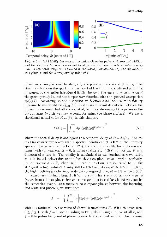
Gate setup
Temporal delay, δt [units of 1/Γ]−10 0 10
1
2
3
4
5
0.2
0.4
0.6
0.8σ [
unit
s of
Γ/vg]
01 2 3 4 5
0
1
Ff
σ [units of Γ/vg]
0.2
0.4
0.6
0.8 (b)(a)
Figure 6.3: (a) Fidelity between an incoming Gaussian pulse with spectral width 𝜎and the state scattered on a resonant two-level emitter close to a terminated waveg-uide. A temporal delay, 𝛿𝑡, is allowed in the fidelity calculation. (b) The maximal 𝐹at a given 𝜎 and the corresponding value of 𝑓 .
phase, as we may account for delays by the phase shifters in the ’0’ arms). Thesimilarity between the spectral wavepacket of the input and scattered photon ismeasured by the earlier introduced fidelity between the spectral wavefunction ofthe gate input, 𝜉(𝑘), and the output wavefunction with the spectral wavepacket𝑡(𝑘)𝜉(𝑘). According to the discussion in Section 5.2.1, the relevant fidelitymeasure to use would be 𝐹spat(𝛿𝑧), as it takes spectral deviations between thepulses into account, but allows a spatial/temporal detuning of the pulses in theoutput arms (which we may account for using the phase shifters). We use ashorthand notation for 𝐹spat(𝛿𝑧) in this chapter,
𝐹 (𝛿𝑧) =
∫ ∞
−∞d𝑝 𝑡(𝑝)|𝜉(𝑝)|2ei𝛿𝑧 · 𝑝
2(6.5)
where the spatial delay is analogous to a temporal delay of 𝛿𝑡 = 𝛿𝑧/𝑣𝑔. Assum-ing Gaussian wavepackets with a spectral bandwidth (FWHM of the intensityspectrum) of 𝜎 as given in Eq. (3.12b), the resulting fidelity for a photon res-onant with the emitter, ∆ = 0, is illustrated in Fig. 6.3(a) by plotting 𝐹 as afunction of 𝜎 and 𝛿𝑡. The fidelity is maximized in the continuous wave limit,𝜎 → 0, for all delays due to the fact that two plane waves overlap perfectly.In the regime 𝜎 ∼ Γ, where non-linear interactions are expected to be thestrongest, a high value of 𝐹 may still be achieved. As expected from Eq. (6.3),the high fidelities are obtained at delays corresponding to 𝛿𝑡 ∼ 4/Γ when 𝜎 . Γ.
Apart from having a large 𝐹 , it is important that the phase across the pulse(apart from a linear phase change - corresponding to a delay) is not changes bythe scattering event. As a measure to compare phases between the incomingand scattered photons, we introduce
𝑓 =1
4
∫ ∞
−∞d𝑝
𝜉(𝑝) + 𝑡(𝑝)𝜉(𝑝)ei𝑣𝑔𝛿𝑡 · 𝑝
2. (6.6)
which is evaluated at the value of 𝛿𝑡 which maximizes 𝐹 . With this measure,0 ≤ 𝑓 ≤ 1, with 𝑓 = 1 corresponding to two pulses being in phase at all 𝑘, and𝑓 = 0 to pulses being out of phase by exactly 𝜋 at all values of 𝑘. The maximal
65
Chapter 6. Controlled phase gate
value of 𝐹 at a specific 𝜎 is plotted together with 𝑓 in Fig. 6.3(b) as a functionof 𝜎. For small values of 𝜎, 𝑓 is close to zero, as expected from Eq. (6.3), asthe scattered pulse attains a constant phase of 𝜋 upon scattering.
Summarizing the linear scattering results, a single photon in one of the ’1’-arms attains a phase shift of 𝜋 and a temporal delay. The linear operationswork optimally when the spectral width of the incoming pulses is much smallerthan the emitter linewidth. In the regime, where the non-linearities may beaddressed the best 𝜎 ∼ Γ, the pulse spectrum is still preserved with more than95% fidelity as seen in Fig. 6.3, if we choose the optimal delays for the emitter-induced temporal delay. This may be done by tuning the induced delay in thephase shifters to match the emitter-induced delay.
6.2.2 Non-linear gate interactions
The non-linear interaction occurs for the input state |”1𝑐”⟩|”1𝑠”⟩. The non-linear scattering is treated in the same way as in Chapter 5, but here we areconsidering a chiral waveguide [66], and we take the directional coupler intoaccount when calculating the scattered state of the entire gate. The gate inputfor two uncorrelated, identical photons and the corresponding gate output are
|𝜓in⟩ =
∫ ∞
−∞d𝑘∫ ∞
−∞d𝑘′ 𝜉(𝑘)𝜉(𝑘′)𝑎†𝑐1(𝑘)𝑎†𝑠1(𝑘′)|𝜑⟩
→ |𝜓scat⟩ = −∫ ∞
−∞d𝑝∫ ∞
−∞d𝑝′ 𝛽scat(𝑝, 𝑝
′)𝑎†𝑐1(𝑝)𝑎†𝑠1(𝑝′)|𝜑⟩ (6.7)
with
𝛽scat(𝑝, 𝑝′) = 𝛽linearscat (𝑝, 𝑝′) +
1
2𝑏(𝑝, 𝑝′) (6.8)
with the linear contribution 𝛽linearscat (𝑝, 𝑝′) = 𝑡(𝑝)𝑡(𝑝′)𝜉(𝑝)𝜉(𝑝′) and a non-linearscattering contribution with
𝑏(𝑝, 𝑝) =
∫ ∞
−∞d𝑘 𝜉(𝑝)𝜉(𝑝′)𝐵𝑝𝑝′𝑘(𝑝+𝑝′−𝑘) (6.9)
where 𝐵𝑝𝑝′𝑘(𝑝+𝑝′−𝑘) is defined in Eq. (5.33).For the c-phase gate to work properly, the scattered state of Eq. (6.7) must
differ by an overall phase of 𝜋 compared to the linear case, where the twophotons do not interact, i.e. to a scattered state as in Eq. (6.7) but with𝛽linearscat (𝑝, 𝑝′) instead of 𝛽scat(𝑝, 𝑝′). As before, the pulse spectrum must alsoremain unchanged. To quantify the scattering-induced effects, we employ two-photon versions of the fidelities from Eqs. (6.5) and (6.6),
𝐹 =
∫ ∞
−∞d𝑝∫ ∞
−∞d𝑝′
[𝛽linearscat (𝑝, 𝑝′)
]*𝛽scat(𝑝, 𝑝
′)ei𝑣𝑔𝛿𝑡(𝑝+𝑝′)
2(6.10)
taking into account that each photon may be delayed by an identical temporaldelay of 𝛿𝑡, and
𝑓 =1
4
∫ ∞
−∞d𝑝∫ ∞
−∞d𝑝′𝛽scat(𝑝, 𝑝
′) + 𝛽linearscat (𝑝, 𝑝′)ei𝑣𝑔(𝑝+𝑝′)𝛿𝑡
2(6.11)
66
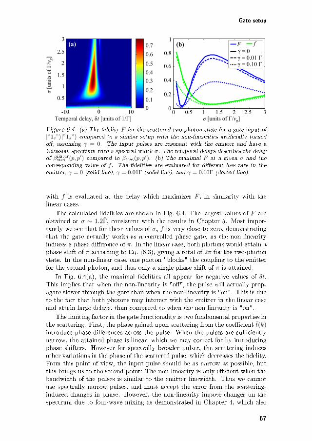
Gate setup
Temporal8delay,8δt8[units8of81/Γ]
σ8[
unit
s8of
8Γ/vg]8
3
2.5
2
1.5
1
0.5
-10 0 100
0.1
0.2
0.3
0.4
0.5
0.6
0.7
32100
0.2
0.4
0.6
0.8
1
σ8[units8of8Γ/vg]8
F
γ8=80γ8=80.018Γγ8=80.108Γ
f
0.5 1.5 2.5
(a) (b)
Figure 6.4: (a) The fidelity 𝐹 for the scattered two-photon state for a gate input of|”1𝑐”⟩|”1𝑠”⟩ compared to a similar setup with the non-linearities artificially turnedoff, assuming 𝛾 = 0. The input pulses are resonant with the emitter and have aGaussian spectrum with a spectral width 𝜎. The temporal delays describes the delayof 𝛽linear
scat (𝑝, 𝑝′) compared to 𝛽scat(𝑝, 𝑝′). (b) The maximal 𝐹 at a given 𝜎 and the
corresponding value of 𝑓 . The fidelities are evaluated for different loss rate in theemitter, 𝛾 = 0 (solid line), 𝛾 = 0.01Γ (solid line), and 𝛾 = 0.10Γ (dotted line).
with 𝑓 is evaluated at the delay which maximizes 𝐹 , in similarity with thelinear cases.
The calculated fidelities are shown in Fig. 6.4. The largest values of 𝐹 areobtained at 𝜎 ∼ 1.2Γ, consistent with the results in Chapter 5. Most impor-tantly we see that for these values of 𝜎, 𝑓 is very close to zero, demonstratingthat the gate actually works as a controlled phase gate, as the non-linearityinduces a phase difference of 𝜋. In the linear case, both photons would attain aphase shift of 𝜋 according to Eq. (6.3), giving a total of 2𝜋 for the two-photonstate. In the non-linear case, one photon "blocks" the coupling to the emitterfor the second photon, and thus only a single phase shift of 𝜋 is attained.
In Fig. 6.4(a), the maximal fidelities all appear for negative values of 𝛿𝑡.This implies that when the non-linearity is "off", the pulse will actually prop-agate slower through the gate than when the non-linearity is "on". This is dueto the fact that both photons may interact with the emitter in the linear caseand attain large delays, than compared to when the non-linearity is "on".
The limiting factor in the gate functionality is two fundamental properties inthe scattering. First, the phase gained upon scattering from the coefficient 𝑡(𝑘)introduce phase differences across the pulse. When the pulses are sufficientlynarrow, the attained phase is linear, which we may correct for by introducingphase shifters. However for spectrally broader pulser, the scattering inducesother variations in the phase of the scattered pulse, which decreases the fidelity.From this point of view, the input pulse should be as narrow as possible, butthis brings us to the second point: The non-linearity is only efficient when thebandwidth of the pulses is similar to the emitter linewidth. Thus we cannotuse spectrally narrow pulses, and must accept the error from the scattering-induced changes in phase. However, the non-linearity impose changes on thespectrum due to four-wave mixing as demonstrated in Chapter 4, which also
67
Chapter 6. Controlled phase gate
results in lower gate fidelities.In the optimal case, the fidelity becomes almost 80 %, as shown Fig. 6.1(b),
when accounting for the non-linearity-induced change in the pulse shape andphase. When taking emitter losses into account, 𝐹 decreases even further, andfor loss rates of 𝛾 = 0.1Γ, 𝐹 is reduced to 40%. Thus it is very importantto effectively couple the emitter to the waveguide. For a semiconductor quan-tum dot inside a photonic crystal waveguide, coupling efficiencies between theemitter and the waveguide of up to 98% has been achieved [45].
6.3 Summary
We have proposed a setup for a deterministic controlled phase gate for twoidentical, uncorrelated single photon pulses, which exploits the intrinsic non-linearity of two-level emitters. Our calculations demonstrate fidelities for thegate operations just below 80%. This is limited by linear scattering-inducedchanges in the phase of the pulse, and also by non-linearity-induced changesin the pulse spectrum and phase, as discussed in Chapter 4. The interactionwith the emitters also causes a delay in the ’1’-arms, but this is accounted forby phase shifters in the ’0’ arms.
The setup depends strongly on having two resonant emitters, which cou-ples with identical strengths to the waveguides. If the emitters are not exactlyidentical, the gate performance would decrease, as it relies on perfect interfer-ence between the states scattered on the two emitters. If only a single emitterwere used in the present setup, only half of the pulse would be affected by thenon-linearity, decreasing the performance of the gate, especially deterioratingthe interference at the directional coupler after the scattering. In standardquantum dot samples, quantum dots are grown at random positions and withdifferent resonant frequencies [61], and thus it may be difficult to fulfil bothcriteria at the same time. Site-controlled growing of the quantum dots has beendemonstrated [135, 136], although it still appears a challenge to precisely con-trol the transition frequencies of the individual dots. Another possibility wouldbe to trap identical atoms close to the facets of the inner waveguides [62, 39],as they by nature would be resonant. This may, however, not be suitable foron-chip integration in larger optical circuits.
As the input and output arms are the same in Fig. 6.2, an implementationof the gate necessitates the use of optical components such as circulators [137]to direct the output into new waveguides. A way to circumvent this is to exploit"uni-directional" non-linearities, i.e. non-linearities which only couple to a sub-set of modes propagating in one direction of the waveguide. With these, thechiral scheme in Fig. 6.2 could be directly implemented. An example of such ischiral spin-photon interfaces, which has recently has been demonstrated experi-mentally for a quantum dot inside a photonic crystal waveguide using polarizedlight [138]. Other candidates are whispering-gallery-type resonators, such asring resonators, microtoroids, microdisks or microspheres [139] created in amaterial with a strong non-linearity (typically a 𝜒(2) non-linearity). As we willdiscuss in the following chapter, recent developments allow fabrication of veryhigh 𝑄-resonator cavities. If the intrinsic non-linearity dominates the losses,
68

Summary
a splitting of the energy spectrum will appear, in similarity with strong cou-pling in an emitter-cavity system. If the coupling between counter-propagatingmodes in the ring is zero, the transmission of a strongly non-linear resonatormay be described by Eq. (6.2), making ring resonators viable candidates forthe proposed gate scheme. Non-linear optical cavities do, however, also sufferfrom the demonstrated non-linear processes which alter the spectrum of thescattered photons [119].
The proposed fidelity of the deterministic gate of almost 80 % is relativelygood, compared to the fact that no external manipulations are required duringthe gate operation, in contrast to many other proposals. The fidelity is, how-ever, difficult to improve further using only passive components, as it is limitby intrinsic properties of the photon scattering.
69

Chapter 7
Controlled phase gate -
Using dynamical capture
The performance of the controlled phase gate in the previous chapter was de-teriorated by side-effects when two photons of the same frequency scatter on anon-linearity at the same time. In this chapter we investigate possibilities of cir-cumventing these side-effects by employing the recently proposed "interaction-free" gate schemes [140, 141], which exploit the quantum Zeno blockade (QZB)[142]. The QZB occurs when frequent or continuous measurements are per-formed on a quantum system, which will inhibit the unitary evolution of thesystem. In optical systems, the "measurements" may be facilitated by a strongoptical non-linear interaction with another photon. We will specifically consideran optical cavity with a large quadratic (𝜒(2)) material non-linearity, giving riseto sum-frequency generation [143]. As will be demonstrated in the following,the presence of one (control) photon in the cavity will prohibit the couplingof another (signal) photon into the cavity, as the control photon continuously"probes" the cavity. In that sense, the QZB is analogous to the photon blockadein a strongly coupled emitter–cavity system [24].
Recently Sun et al. [141] made a theoretical proposal of a c-phase gate,which employs a lithium niobate (LiNbO3) ring resonator, as LiNbO3 has ahigh intrinsic (𝜒(2)) non-linearity. In the scheme, a temporally broad (con-trol) photon probes the cavity during the time where second (signal) photonscatters. When the control is "on", it prohibits the signal for entering thecavity, giving the conditional gate operation and predicts fidelities of up to98 % (although they do not take into account that the temporal shape of thecontrol is reversed). The scheme proposed by Sun et al. does however notwork for identical photons as the gate in Chapter 6, as their proposal relieson using photons of different frequencies. This enables the signal and controlphoton to be distinguished at the output, which would not be possible whenusing two identical photons, and the gate does not seem suitable for large-scaleintegration in general quantum circuits.
A method to overcome this when using two identical photons is proposedin a scheme for a c-phase gate by Johne et al. [129], in which the control
71
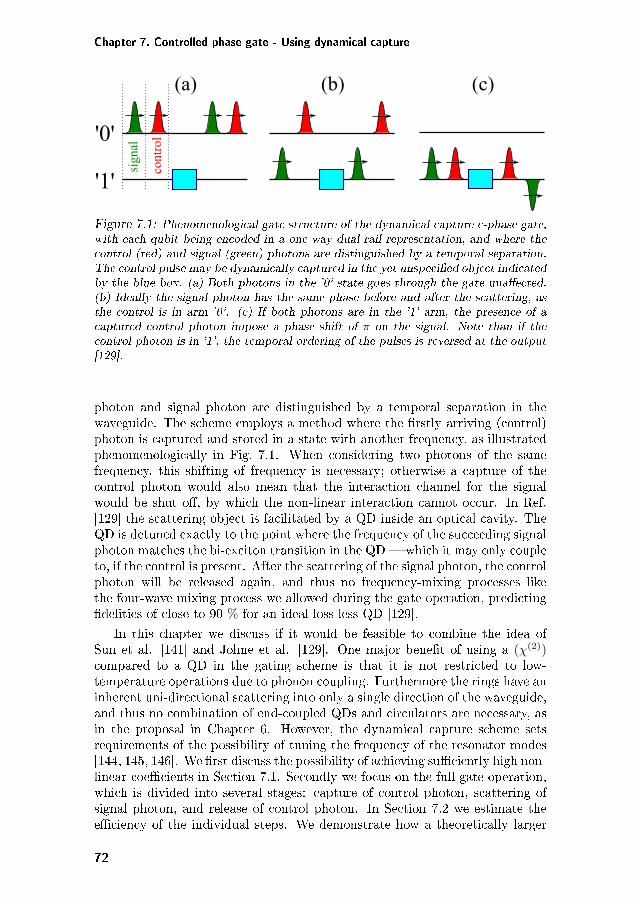
Chapter 7. Controlled phase gate - Using dynamical capture
'0'
'1'
(b)(a)
control
signal
(c)
Figure 7.1: Phenomenological gate structure of the dynamical capture c-phase gate,with each qubit being encoded in a one-way dual-rail representation, and where thecontrol (red) and signal (green) photons are distinguished by a temporal separation.The control pulse may be dynamically captured in the yet unspecified object indicatedby the blue box. (a) Both photons in the ’0’ state goes through the gate unaffected.(b) Ideally the signal photon has the same phase before and after the scattering, asthe control is in arm ’0’. (c) If both photons are in the ’1’ arm, the presence of acaptured control photon impose a phase shift of 𝜋 on the signal. Note than if thecontrol photon is in ’1’, the temporal ordering of the pulses is reversed at the output[129].
photon and signal photon are distinguished by a temporal separation in thewaveguide. The scheme employs a method where the firstly arriving (control)photon is captured and stored in a state with another frequency, as illustratedphenomenologically in Fig. 7.1. When considering two photons of the samefrequency, this shifting of frequency is necessary; otherwise a capture of thecontrol photon would also mean that the interaction channel for the signalwould be shut off, by which the non-linear interaction cannot occur. In Ref.[129] the scattering object is facilitated by a QD inside an optical cavity. TheQD is detuned exactly to the point where the frequency of the succeeding signalphoton matches the bi-exciton transition in the QD— which it may only coupleto, if the control is present. After the scattering of the signal photon, the controlphoton will be released again, and thus no frequency-mixing processes likethe four-wave mixing process we allowed during the gate operation, predictingfidelities of close to 90 % for an ideal loss-less QD [129].
In this chapter we discuss if it would be feasible to combine the idea ofSun et al. [141] and Johne et al. [129]. One major benefit of using a (𝜒(2))compared to a QD in the gating scheme is that it is not restricted to low-temperature operations due to phonon coupling. Furthermore the rings have aninherent uni-directional scattering into only a single direction of the waveguide,and thus no combination of end-coupled QDs and circulators are necessary, asin the proposal in Chapter 6. However, the dynamical capture scheme setsrequirements of the possibility of tuning the frequency of the resonator modes[144, 145, 146]. We first discuss the possibility of achieving sufficiently high non-linear coefficients in Section 7.1. Secondly we focus on the full gate operation,which is divided into several stages: capture of control photon, scattering ofsignal photon, and release of control photon. In Section 7.2 we estimate theefficiency of the individual steps. We demonstrate how a theoretically larger
72
Requirements for ring-resonator non-linearity
fidelity may be obtained using this gate scheme as compared to the passivescheme in Chapter 6, but is also sets high fabricational requirements on thering properties and timing possibilities during the gate operation.
The research presented in this chapter is from an ongoing research collabora-tion with Mikkel Heuck and Prof. Dirk Englund from the Quantum PhotonicsGroup at Massachusetts Institute of Technology.
7.1 Requirements for ring-resonator non-linearity
In this section we estimate the requirements on the magnitude of the non-linearity compared to the losses in order for the QZB scheme to work. To doso, we specifically consider three energies in the ring resonator, 𝜔1, 𝜔2, and 𝜔3 =𝜔1 + 𝜔2, and we assume the that a single non-degenerate mode exists at eachfrequency. In ring resonators, sum-frequency generation may populate the sum-state, but an additional condition apart from conservation of energy has to befulfilled, namely quasi-phase matching (QPM) condition. For disk resonators,QPM is usually obtained by a periodical poling of the disk [147, 148, 141]. Inreality it is possible to obtain a structure with a set of frequencies as statedabove, but it requires numerical (and sometimes analytical, when possible)investigations for the specific structure to find possible sets of 𝜔1, 𝜔2, 𝜔3 [149,150, 141].
Following Ref. [141], the Hamiltonian of the three-mode system may bedescribed by
𝐻 =
3∑𝑗=1
~𝜔𝑗𝑎†𝑗𝑎𝑗 + ~
(𝑈𝑎†3𝑎2𝑎1 + 𝑈*𝑎†1𝑎
†2𝑎3
), (7.1)
where 𝑈 is the non-linear coupling coefficient describing sum-frequency gener-ation between the considered resonator modes. It has the form
𝑈 =𝜒(2)
2
√~𝜔1𝜔2𝜔3
𝜖0
∫𝑉
dr𝐷(r)Φ1(r)Φ2(r)Φ*3(r), (7.2)
with 𝜒(2) being the non-linear coefficient, Φ𝑗(r) the spatial mode profile of mode𝑗, and 𝐷(r) being a function describing the spatial dependence determinedby the fabricated QPM pattern [141, 149]. Thus, a high value of 𝑈 dependon a high value of the non-linear coefficient, but also on the modal overlapbetween the spatial wavefunctions of the three modes. As detailed calculationsof possibly attainable values of 𝑈 are given in Ref. [141] for a LiNbO3 resonator,we will not elaborate further on the calculation details here, but simply referto their calculations.
Eq. (7.1) is derived under a no-loss assumption. However, losses of thecavity system may be included as coupling to external reservoirs for each ofthe three ring modes according to Refs. [149, 70, 151], giving an effectiveHamiltonian on the form
𝐻eff =
3∑𝑗=1
~𝑗𝑎†𝑗𝑎𝑗 + ~
(𝑈𝑎†3𝑎2𝑎1 + 𝑈*𝑎†1𝑎
†2𝑎3
), (7.3)
73
Chapter 7. Controlled phase gate - Using dynamical capture
with 𝑗 = 𝜔𝑗 − i𝛾𝑗/2, where 𝛾𝑗 is the loss rate of energy in mode 𝑗 in theresonator. If the ring is initially populated by two photons, one with frequency𝜔1 and one with frequency 𝜔2, the system state is
|𝜓(𝑡)⟩ = 𝐶12(𝑡)𝑎†1𝑎†2|𝜑⟩ + 𝐶3(𝑡)𝑎†3|𝜑⟩, (7.4)
with |𝜑⟩ describes the vacuum state, and where the expansion coefficient arenot normalized, due to the presence of loss. The temporal evolution of thesystem is determined by the time-dependent Schrödinger equation, i~𝜕𝑡|𝜓(𝑡)⟩ =𝐻eff|𝜓(𝑡)⟩, providing equations of motion for the expansion coefficients,
𝜕𝑡𝐶12(𝑡) = −i(1 + 2)𝐶12 − i𝑈*𝐶3(𝑡), (7.5)
𝜕𝑡𝐶3(𝑡) = −i3𝐶3 − i𝑈𝐶12(𝑡). (7.6)
The corresponding eigenvalues of the differential equation system are
𝜆± = −
⎛⎝i𝜔3 +
3∑𝑗=1
𝛾𝑗4
⎞⎠± i
√|𝑈 |2 −
(𝛾1 + 𝛾2 − 𝛾3
4
)2
. (7.7)
In similarity with the Jaynes Cummings model, two regimes exist describingthe dynamical evolution of the system. If the non-linearity is strong, 4|𝑈 | >𝛾1 + 𝛾2 − 𝛾3, two new non-degenerate eigenstates form, |𝜆−⟩ and |𝜆+⟩, beingsuperpositions between the two states 𝑎†1𝑎
†2|𝜑⟩ and 𝑎†3|𝜑⟩, see Fig. 7.2(a,b).
These levels may be properly resolved if the splitting between the new statesis much larger than the loss-induced broadening, which from Eq. (7.7) occurswhen |𝑈 |2 ≫ [(𝛾1 + 𝛾2)2 + 𝛾23 ]/8. If 𝑈 is sufficiently large as illustrated inFig. 7.2(b), the splitting may be exploited in the c-phase gate in the way, thatwhen a control photon proves the cavity, an incoming signal photon cannotcouple, giving the conditional operation in the gate.
The task is now to determine realistic values for 𝑈 and the loss rates for thisspecific configuration. The needed calculations for the non-linear coefficient ina LiNbO3 resonator have already carried out by Sun et al. in Ref. [141]. Herethe magnitude of the non-linear parameter, 𝑈 , is estimated from the mode pro-files of a whispering gallery mode using Eq. (7.2), based on calculations from[152]. A figure of merit for the non-linear parameter is 𝜒(2)𝑄/𝑉 , with 𝑄 beingthe quality factor of the resonator more and 𝑉 the mode volume. A realisti-cally obtainable value1 of 𝑈 is estimated to be 𝑈 = 337MHz for a disk LiNbO3resonator with a diameter of 40𝜇m, using the available micro-fabrication tech-nology. We assume that one of the loss rates is dominating the others, denotedby 𝛾, e.g. corresponding to a mode which couples to a waveguide mode, as wewill discuss below. For the gate to work properly, a maximum allowed loss rateis 𝛾max = 2
√2|𝑈 |. Assuming that the wavelength of the light is 𝜆 = 1.31𝜇m,
and that the decay rate of all modes is identical, the minimal quality factor ofeach mode must be 𝑄min = 𝜔0/𝛾max = 2𝜋𝑐/(2
√2|𝑈 |𝜆𝑛ref) = 7 × 10⁵, using a
the refractive index of lithium niobate of 𝑛ref = 2.22 [153].
1In Ref. [141] they even use a value of 610 MHz in their theoretical calculations, althoughthis seems large compared to realistically obtained values nowadays. It may, however, bepossible to achieve soon with the rapid improvements in micro- and nanofabrication.
74
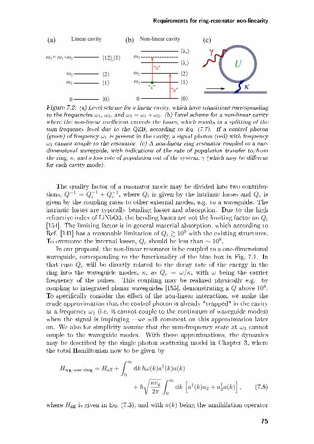
Requirements for ring-resonator non-linearity
ω2
ω1
ω3= ω1+ω2
0 0
1
2
12
ω2
ω1
0 0
1
2
λ-
λ+
"c"
"s"
"s"
ω33,
Linear cavity Non-linear cavity
κ
U
γ(a) (b) (c)
Figure 7.2: (a) Level scheme for a linear cavity, which have transitions correspondingto the frequencies 𝜔1, 𝜔2, and 𝜔3 = 𝜔1 +𝜔2. (b) Level scheme for a non-linear cavitywhere the non-linear coefficient exceeds the losses, which results in a splitting of thesum-frequency level due to the QZB, according to Eq. (7.7). If a control photon(green) of frequency 𝜔1 is present in the cavity, a signal photon (red) with frequency𝜔2 cannot couple to the resonator. (c) A non-linear ring resonator coupled to a one-dimensional waveguide, with indications of the rate of population transfer to/fromthe ring, 𝜅, and a loss rate of population out of the system, 𝛾 (which may be differentfor each cavity mode).
The quality factor of a resonator mode may be divided into two contribu-tions, 𝑄−1 = 𝑄−1
𝑖 + 𝑄−1𝑐 , where 𝑄𝑖 is given by the intrinsic losses and 𝑄𝑐 is
given by the coupling rates to other external modes, e.g. to a waveguide. Theintrinsic losses are typically bending losses and absorption. Due to the highrefractive index of LiNbO3, the bending losses are not the limiting factor on 𝑄𝑖
[154]. The limiting factor is in general material absorption, which according toRef. [141] has a reasonable limitation of 𝑄𝑖 & 109 with the existing structures.To overcome the internal losses, 𝑄𝑐 should be less than ∼ 108.
In our proposal, the non-linear resonator is be coupled to a one-dimensionalwaveguide, corresponding to the functionality of the blue box in Fig. 7.1. Inthat case 𝑄𝑐 will be directly related to the decay rate of the energy in thering into the waveguide modes, 𝜅, as 𝑄𝑐 = 𝜔/𝜅, with 𝜔 being the carrierfrequency of the pulses. This coupling may be realized physically e.g. bycoupling to integrated planar waveguides [155], demonstrating a 𝑄 above 108.To specifically consider the effect of the non-linear interaction, we make thecrude approximation that the control photon is already "trapped" in the cavityat a frequency 𝜔1 (i.e. it cannot couple to the continuum of waveguide modes)when the signal is impinging – we will comment on this approximation lateron. We also for simplicity assume that the sum-frequency state at 𝜔3 cannotcouple to the waveguide modes. With these approximations, the dynamicsmay be described by the single-photon scattering model in Chapter 3, wherethe total Hamiltonian now to be given by
𝐻wg–one ring = 𝐻eff +
∫ ∞
0
d𝑘 ~𝜔(𝑘)𝑎†(𝑘)𝑎(𝑘)
+ ~√𝜅𝑣𝑔2𝜋
∫ ∞
0
d𝑘[𝑎†(𝑘)𝑎2 + 𝑎†2𝑎(𝑘)
], (7.8)
where 𝐻eff is given in Eq. (7.3), and with 𝑎(𝑘) being the annihilation operator
75
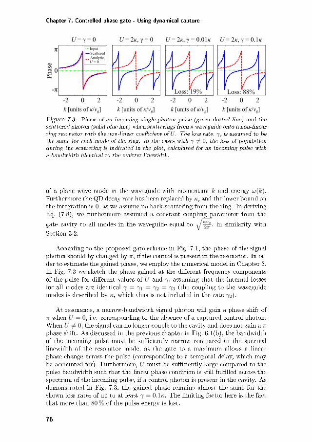
Chapter 7. Controlled phase gate - Using dynamical capture
π
-π
0
Pha
se
-2 0 2kL[unitsLofLκ/vg]L
-2 0 2kL[unitsLofLκ/vg]L
-2 0 2kL[unitsLofLκ/vg]L
-2 0 2kL[unitsLofLκ/vg]L
UL=LγL=L0 UL=L2κ,LγL=L0 UL=L2κ,LγL=L0.01κInputScatteredAnalytic,UL=L0
UL=L2κ,LγL=L0.1κ
Loss:L88%Loss:L19%
Figure 7.3: Phase of an incoming single-photon pulse (green dotted line) and thescattered photon (solid blue line) when scatterings from a waveguide onto a non-linearring resonator with the non-linear coefficient of 𝑈 . The loss rate, 𝛾, is assumed to bethe same for each mode of the ring. In the cases with 𝛾 = 0, the loss of populationduring the scattering is indicated in the plot, calculated for an incoming pulse witha bandwidth identical to the emitter linewidth.
of a plane wave mode in the waveguide with momentum 𝑘 and energy 𝜔(𝑘).Furthermore the QD decay rate has been replaced by 𝜅, and the lower bound onthe integration is 0, as we assume no back-scattering from the ring. In derivingEq. (7.8), we furthermore assumed a constant coupling parameter from the
gate cavity to all modes in the waveguide equal to√
𝜅𝑣𝑔2𝜋 , in similarity with
Section 3.2.
According to the proposed gate scheme in Fig. 7.1, the phase of the signalphoton should by changed by 𝜋, if the control is present in the resonator. In or-der to estimate the gained phase, we employ the numerical model in Chapter 3.In Fig. 7.3 we sketch the phase gained at the different frequency componentsof the pulse for different values of 𝑈 and 𝛾, assuming that the internal lossesfor all modes are identical 𝛾 = 𝛾1 = 𝛾2 = 𝛾3 (the coupling to the waveguidemodes is described by 𝜅, which thus is not included in the rate 𝛾2).
At resonance, a narrow-bandwidth signal photon will gain a phase shift of𝜋 when 𝑈 = 0, i.e. corresponding to the absence of a captured control photon.When 𝑈 = 0, the signal can no longer couple to the cavity and does not gain a 𝜋phase shift. As discussed in the previous chapter in Fig. 6.1(b), the bandwidthof the incoming pulse must be sufficiently narrow compared to the spectrallinewidth of the resonator mode, as the gate to a maximum allows a linearphase change across the pulse (corresponding to a temporal delay, which maybe accounted for). Furthermore, 𝑈 must be sufficiently large compared to thepulse bandwidth such that the linear phase condition is still fulfilled across thespectrum of the incoming pulse, if a control photon is present in the cavity. Asdemonstrated in Fig. 7.3, the gained phase remains almost the same for theshown loss rates of up to at least 𝛾 = 0.1𝜅. The limiting factor here is the factthat more than 80 % of the pulse energy is lost.
76
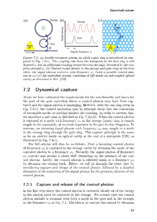
Dynamical capture
g
κσ
U
σ
κ
g
Mod
al d
ensi
ty
Angular frequency, ω
ω1 ω2
Storage
Gate
(a) (b) (c)Storage
Gate
Figure 7.4: (a) Double-resonator system, in which a gate ring is introduced as com-pared to Fig. 7.2(c). The coupling rate from the waveguide to the first ring is stilldenoted 𝜅, but an additional coupling occurs between the rings, described by the cou-pling strength 𝑔. (b) Desired modal density in the storage and gate rings at the timewhere the signal photon scatteres with frequency 𝜔1 (with a possible control pho-ton at 𝜔2) (c) An equivalent system, consisting of QD inside an end-coupled opticalcavity, as described in Ref. [129].
7.2 Dynamical capture
Above we have estimated the requirements for the non-linearity and losses forthe part of the gate operation where a control photon may have been cap-tured and the signal photon is impinging. However, with the one-ring setup inFig. 7.2(c), the control excitation may in principle decay into the continuumof waveguide modes as nothing hinders the coupling. In order to prevent this,we introduce a gate-ring as sketched in Fig. 7.4(a,b). When the control photonis captured at a mode with frequency 𝜔1 in the storage (inner) ring, it cannotcouple to the waveguide, as no mode is present in the gate at that frequency. Incontrast, an incoming signal photon with frequency 𝜔2 may couple to a modein the storage ring through the gate ring. This capture principle is the sameas for an emitter inside an optical cavity at the end of a waveguide [129], asillustrated in Fig. 7.4(c).
The full scheme will thus be as follows: First a incoming control photonof frequency 𝜔2 is captured in the storage cavity by detuning the mode of thecaptured photon to a frequency 𝜔1. Secondly, the signal photon of frequency𝜔2 scatters and attains a phase shift depending on the presence of the con-trol photon. Lastly, the control photon is released again at a frequency 𝜔2
by detuning the storage back. Below, we will go through the steps; first byconsidering capture and release of the control photon, followed by a detaileddiscussion of the scattering of the signal photon for the presence/absence of thecontrol photon.
7.2.1 Capture and release of the control photon
In the first step where the control photon is captured, ideally all of the energyin the photon must be captured in the storage. We assume that the controlphoton initially is resonant with both a mode in the gate and in the storage,at the frequency 𝜔2 in Fig. 7.4. The idea is to capture the control by detuning
77
Chapter 7. Controlled phase gate - Using dynamical capture
the storage exactly when it is populated the most. Here we only consider thepossibility of tuning the resonances of the storage. In that case, the controlphoton must have a specific spectral and temporal shape in order to be fullyabsorbed. The optimal may be determined by reversing the capture process,i.e. by determining the pulse shape of an emitted photon if the storage initiallyis excited.
To determine this, we define a Hamiltonian for the double-ring system validfor a single excitation, in analogy with the derivations in Chapter 3,
𝐻wg–double-ring = ~𝑔(𝑎†s𝑎g + 𝑎†g𝑎s) + ~√𝜅𝑣𝑔2𝜋
∫ ∞
0
d𝑘[𝑎†(𝑘)𝑎g + 𝑎†g𝑎(𝑘)
], (7.9)
with 𝑎s and 𝑎g being annihilation operators for the considered mode in thestorage and gate resonator, respectively (we do not include transitions to othermodes here). The coupling rate 𝑔 is proportional to the rate at which energyis transferred between the rings. The single-excitation state of the system is
|𝜓(𝑡)⟩ = 𝐶s(𝑡)𝑎†s |𝜑⟩ + 𝐶g(𝑡)𝑎
†g|𝜑⟩ +
∫ ∞
0
d𝑘 𝐶wg(𝑘, 𝑡)𝑎†(𝑘, 𝑡)|𝜑⟩, (7.10)
with |𝐶s/g(𝑡)|2 being the population in the storage/gate ring at time 𝑡, and
with∫ 𝑘2
𝑘1d𝑘 |𝐶wg(𝑘, 𝑡)|2 being the possibility having a photon with momentum
between 𝑘1 and 𝑘2 > 𝑘1 at time 𝑡. In a similar way as in Chapter 3, we use thetime-independent Schrödinger equation to determine differential equations forthe expansion coefficients. In a frame rotating with the frequency of the modesin the gate and storage, which is assumed to be the same, we arrive at
𝜕𝑡𝐶s(𝑡) = −i𝑔𝐶g(𝑡), (7.11a)
𝜕𝑡𝐶g(𝑡) = −𝜅2𝐶g(𝑡) − i𝑔𝐶s(𝑡), (7.11b)
where the coupling to the waveguide modes may described by 𝜅 mode withnarrow linewidths compared to the carrier frequencies of the pulses, in analogyto Γ in Eq. (3.9). By solving these equations, the spontaneously emitted pulseshape is given by the temporal wavepacket
𝜉(𝑡) = i𝑔√𝜅
𝐽e−𝜅𝑡/4
[ei𝐽𝑡/2 − e−i𝐽𝑡/2
], (7.12)
where 𝐽 =√
4𝑔2 − 𝜅2/4 is either real or purely imaginary, depending on if thesystem is in the strong or weak coupling regime, respectively.
Using the numerical approach in Section 3.3 with a temporally reversedversion of Eq. (7.12) as input, we calculate the full scattering dynamics, seeFig. 7.5. In Fig. 7.5(a), the resulting gate and storage populations are shown.The idea is to detune the storage exactly when the population of the stor-age is at its maximum, here 𝑡/𝜅 ∼ 13. To illustrate the scattering dynam-ics clearly, we evaluate the spectral density in the waveguide, 𝑁𝑘(𝑘, 𝑡) =⟨𝜓(𝑡)|𝑎†(𝑘)𝑎(𝑘)|𝜓(𝑡)⟩, and the spatial photon density in the waveguide, 𝑁𝑧(𝑧, 𝑡),given in Eq. (3.15). These are plotted in Fig. 7.5(b,c), and specifically we no-tice, that the temporal shape of the pulse is reversed for the scattered pulse.
78
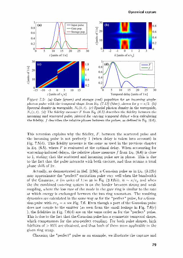
Dynamical capture
Ff
-3 -2 -1 0 1 2 30
10
20
30
0
0.2
0.4
0.6
0.8
-15 -10 -5 0 5 10 15
0 5 10 15 20 25 300
0.2
0.4
0.6
0.8
1
tm[unitsmofm1/κ]
InputmpulseGatempop.Storagempop.
km[unitsmofmκ/vg]
tm[un
itsm
ofm1
/κ]
zm[unitsmofmvg/κ] Temporalmdelaym[unitsmofm1/κ]0 5 10 15 20 25 30
0
10
20
30
tm[un
itsm
ofm1
/κ]
0
0.2
0.4
0.6
0.8
1
0.2
0.6
1
1.4
1.8
(a)
(d)(c)
(b)
Figure 7.5: (a) Gate (green) and storage (red) popultion for an incoming single-photon pulse with the temporal shape from Eq. (7.12) (blue), shown for 𝑔 = 𝜅/2. (b)Spectral density in waveguide, 𝑁𝑘(𝑘, 𝑡). (c) Spatial photon density in the waveguide,𝑁𝑧(𝑧, 𝑡). (d) The fidelity measure 𝐹 from Eq. (6.5) describes the fidelity between theincoming and scattered pulse, plotted for varying temporal delays when calculatingthe fidelity. 𝑓 describes the relative phases between the pulses, as defined in Eq. (6.6).
This reversion explains why the fidelity, 𝐹 , between the scattered pulse andthe incoming pulse is not perfectly 1 (when delay is taken into account) inFig. 7.5(d). This fidelity measure is the same as used in the previous chapterin Eq. (6.5), where 𝐹 is evaluated at the optimal delay. When accounting forscattering-induced delays, the relative phase measure 𝑓 from Eq. (6.6) is closeto 1, stating that the scattered and incoming pulse are in phase. This is dueto the fact that the pulse interacts with both cavities, and thus attains a totalphase shift of 2𝜋.
Actually, as demonstrated in Ref. [156], a Gaussian pulse as in Eq. (3.12b)may approximate the "perfect" excitation pulse very well when the bandwidthof the Gaussian, 𝜎 (in units of 1/m as in Eq. (3.12b)), is ∼ 𝜅/𝑣𝑔 and whenthe the combined two-ring system is on the border between strong and weakcoupling, where the loss rate of the mode in the gate ring is similar to the rateat which energy is exchanged between the two ring resonators. The resultingdynamics are calculated in the same way as for the "perfect" pulse, for a Gaus-sian pulse with 𝜎𝑣𝑔 = 𝜅 see Fig. 7.6. Even though a part of the Gaussian pulsedoes not couple to the emitter (as seen from the small leakage in Fig. 7.6(c)), the fidelities in Fig. 7.6(d) are on the same order as for the "perfect" pulse.This is due to the fact that the Gaussian pulse has a symmetric temporal shape,which compensates for the non-perfect coupling. For both pulse shapes, highfidelities of > 95% are obtained, and thus both of them seem applicable in thegiven ring setup.
Choosing the "perfect" pulse as an example, we illustrate the capture and
79
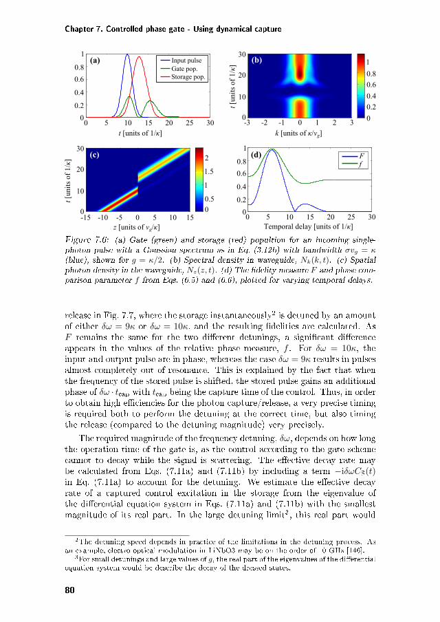
Chapter 7. Controlled phase gate - Using dynamical capture
-3 -2 -1 0 1 2 30
10
20
30
0
0.2
0.4
0.6
0.8
-15 -10 -5 0 5 10 15
0 5 10 15 20 25 300
0.2
0.4
0.6
0.8
1
tm[unitsmofm1/κ]
InputmpulseGatempop.Storagempop.
km[unitsmofmκ/vg]
tm[un
itsm
ofm1
/κ]
zm[unitsmofmvg/κ]0 5 10 15 20 25 30
0
10
20
30
tm[un
itsm
ofm1
/κ]
0
0.2
0.4
0.6
0.8
1
0
0.5
1
1.5
2
(a)
(d)(c)
(b) 1
Ff
Temporalmdelaym[unitsmofm1/κ]
Figure 7.6: (a) Gate (green) and storage (red) popultion for an incoming single-photon pulse with a Gaussian spectrum as in Eq. (3.12b) with bandwidth 𝜎𝑣𝑔 = 𝜅(blue), shown for 𝑔 = 𝜅/2. (b) Spectral density in waveguide, 𝑁𝑘(𝑘, 𝑡). (c) Spatialphoton density in the waveguide, 𝑁𝑧(𝑧, 𝑡). (d) The fidelity measure 𝐹 and phase com-parison parameter 𝑓 from Eqs. (6.5) and (6.6), plotted for varying temporal delays.
release in Fig. 7.7, where the storage instantaneously2 is detuned by an amountof either 𝛿𝜔 = 9𝜅 or 𝛿𝜔 = 10𝜅, and the resulting fidelities are calculated. As𝐹 remains the same for the two different detunings, a significant differenceappears in the values of the relative phase measure, 𝑓 . For 𝛿𝜔 = 10𝜅, theinput and output pulse are in phase, whereas the case 𝛿𝜔 = 9𝜅 results in pulsesalmost completely out of resonance. This is explained by the fact that whenthe frequency of the stored pulse is shifted, the stored pulse gains an additionalphase of 𝛿𝜔 · 𝑡cap with 𝑡cap being the capture time of the control. Thus, in orderto obtain high efficiencies for the photon capture/release, a very precise timingis required both to perform the detuning at the correct time, but also timingthe release (compared to the detuning magnitude) very precisely.
The required magnitude of the frequency detuning, 𝛿𝜔, depends on how longthe operation time of the gate is, as the control according to the gate schemecannot to decay while the signal is scattering. The effective decay rate maybe calculated from Eqs. (7.11a) and (7.11b) by including a term −i𝛿𝜔𝐶S(𝑡)in Eq. (7.11a) to account for the detuning. We estimate the effective decayrate of a captured control excitation in the storage from the eigenvalue ofthe differential equation system in Eqs. (7.11a) and (7.11b) with the smallestmagnitude of its real part. In the large detuning limit3, this real part would
2The detuning speed depends in practice of the limitations in the detuning process. Asan example, electro-optical modulation in LiNbO3 may be on the order of 10 GHz [146].
3For small detunings and large values of 𝑔, the real part of the eigenvalues of the differentialequation system would be describe the decay of the dressed states.
80
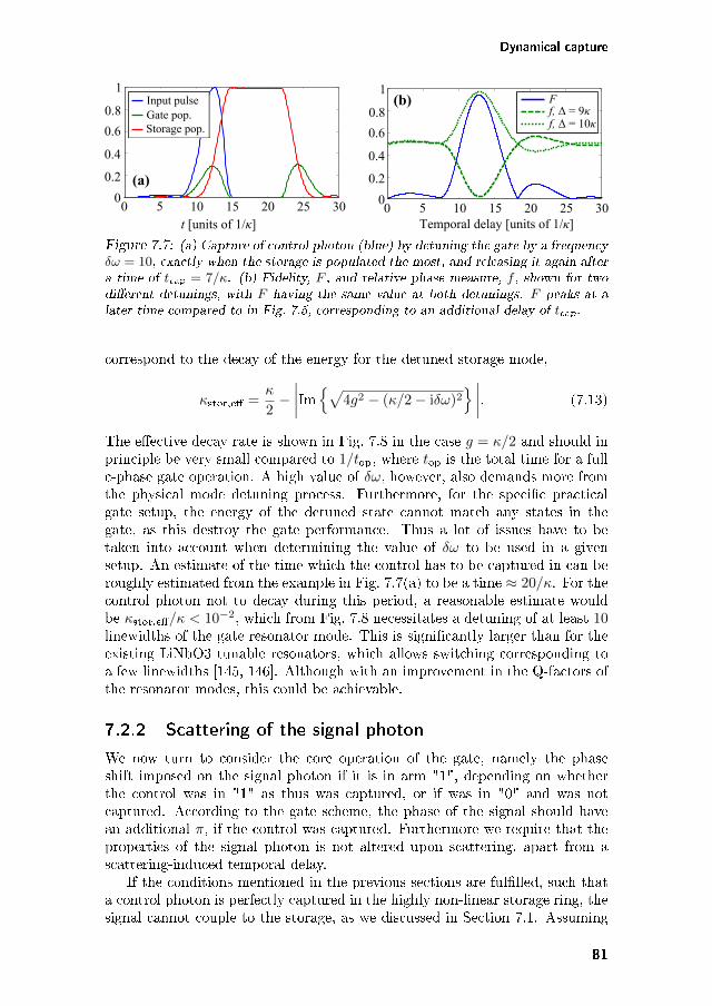
Dynamical capture
0 5 10 15 20 25 300
0.2
0.4
0.6
0.8
1
tS[unitsSofS1/κ] TemporalSdelayS[unitsSofS1/κ]0 5 10 15 20 25 30
0
0.2
0.4
0.6
0.8
1
(a)
InputSpulseGateSpop.StorageSpop.
Ff, ΔS=S9κf, ΔS=S10κ
(b)
Figure 7.7: (a) Capture of control photon (blue) by detuning the gate by a frequency𝛿𝜔 = 10, exactly when the storage is populated the most, and releasing it again aftera time of 𝑡cap = 7/𝜅. (b) Fidelity, 𝐹 , and relative phase measure, 𝑓 , shown for twodifferent detunings, with 𝐹 having the same value at both detunings. 𝐹 peaks at alater time compared to in Fig. 7.5, corresponding to an additional delay of 𝑡cap.
correspond to the decay of the energy for the detuned storage mode,
𝜅stor,eff =𝜅
2−Im√
4𝑔2 − (𝜅/2 − i𝛿𝜔)2 . (7.13)
The effective decay rate is shown in Fig. 7.8 in the case 𝑔 = 𝜅/2 and should inprinciple be very small compared to 1/𝑡op, where 𝑡op is the total time for a fullc-phase gate operation. A high value of 𝛿𝜔, however, also demands more fromthe physical mode detuning process. Furthermore, for the specific practicalgate setup, the energy of the detuned state cannot match any states in thegate, as this destroy the gate performance. Thus a lot of issues have to betaken into account when determining the value of 𝛿𝜔 to be used in a givensetup. An estimate of the time which the control has to be captured in can beroughly estimated from the example in Fig. 7.7(a) to be a time ≈ 20/𝜅. For thecontrol photon not to decay during this period, a reasonable estimate wouldbe 𝜅stor,eff/𝜅 < 10−2, which from Fig. 7.8 necessitates a detuning of at least 10linewidths of the gate resonator mode. This is significantly larger than for theexisting LiNbO3 tunable resonators, which allows switching corresponding toa few linewidths [145, 146]. Although with an improvement in the Q-factors ofthe resonator modes, this could be achievable.
7.2.2 Scattering of the signal photon
We now turn to consider the core operation of the gate, namely the phaseshift imposed on the signal photon if it is in arm "1", depending on whetherthe control was in "1" as thus was captured, or if was in "0" and was notcaptured. According to the gate scheme, the phase of the signal should havean additional 𝜋, if the control was captured. Furthermore we require that theproperties of the signal photon is not altered upon scattering, apart from ascattering-induced temporal delay.
If the conditions mentioned in the previous sections are fulfilled, such thata control photon is perfectly captured in the highly non-linear storage ring, thesignal cannot couple to the storage, as we discussed in Section 7.1. Assuming
81
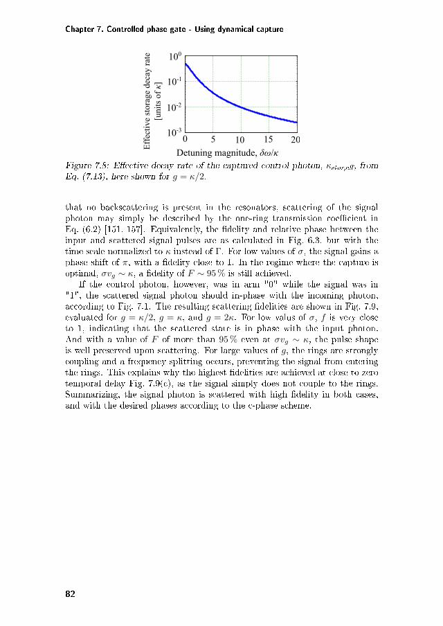
Chapter 7. Controlled phase gate - Using dynamical capture
100
10-1
10-2
10-3
Detuning magnitude, δω/κ E
ffec
tive
sto
rage
dec
ay r
ate
[uni
ts o
f κ]
0 5 10 15 20
Figure 7.8: Effective decay rate of the captured control photon, 𝜅stor,eff, fromEq. (7.13), here shown for 𝑔 = 𝜅/2.
that no backscattering is present in the resonators, scattering of the signalphoton may simply be described by the one-ring transmission coefficient inEq. (6.2) [151, 157]. Equivalently, the fidelity and relative phase between theinput and scattered signal pulses are as calculated in Fig. 6.3, but with thetime scale normalized to 𝜅 instead of Γ. For low values of 𝜎, the signal gains aphase shift of 𝜋, with a fidelity close to 1. In the regime where the capture isoptimal, 𝜎𝑣𝑔 ∼ 𝜅, a fidelity of 𝐹 ∼ 95 % is still achieved.
If the control photon, however, was in arm "0" while the signal was in"1", the scattered signal photon should in-phase with the incoming photon,according to Fig. 7.1. The resulting scattering fidelities are shown in Fig. 7.9,evaluated for 𝑔 = 𝜅/2, 𝑔 = 𝜅, and 𝑔 = 2𝜅. For low valus of 𝜎, 𝑓 is very closeto 1, indicating that the scattered state is in phase with the input photon.And with a value of 𝐹 of more than 95 % even at 𝜎𝑣𝑔 ∼ 𝜅, the pulse shapeis well preserved upon scattering. For large values of 𝑔, the rings are stronglycoupling and a frequency splitting occurs, preventing the signal from enteringthe rings. This explains why the highest fidelities are achieved at close to zerotemporal delay Fig. 7.9(c), as the signal simply does not couple to the rings.Summarizing, the signal photon is scattered with high fidelity in both cases,and with the desired phases according to the c-phase scheme.
82
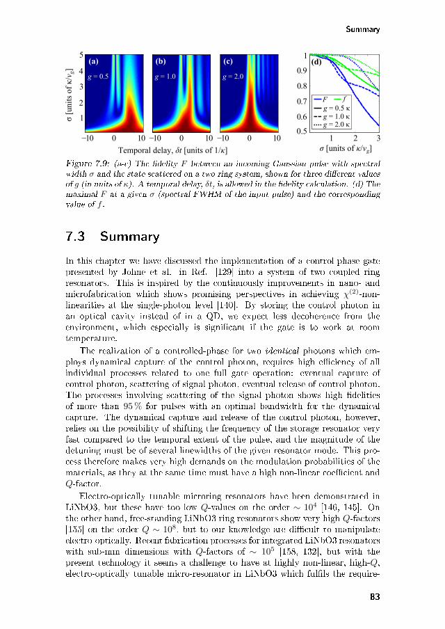
Summary
1 2 30.5
1
σ4[units4of4κ/vg]4
0.6
0.7
0.8
0.9
Temporal4delay,4δt4[units4of41/κ]
−10 0 10 −10 0 10 −10 0 10
1
2
3
4
5
σ4[u
nits
4of4κ/
v g]4
(a) (b) (c)
F
g =40.54κg =41.04κg =42.04κ
f
g =40.5 g =41.0 g =42.0
(d)
Figure 7.9: (a-c) The fidelity 𝐹 between an incoming Gaussian pulse with spectralwidth 𝜎 and the state scattered on a two-ring system, shown for three different valuesof 𝑔 (in units of 𝜅). A temporal delay, 𝛿𝑡, is allowed in the fidelity calculation. (d) Themaximal 𝐹 at a given 𝜎 (spectral FWHM of the input pulse) and the correspondingvalue of 𝑓 .
7.3 Summary
In this chapter we have discussed the implementation of a control-phase gatepresented by Johne et al. in Ref. [129] into a system of two coupled ringresonators. This is inspired by the continuously improvements in nano- andmicrofabrication which shows promising perspectives in achieving 𝜒(2)-non-linearities at the single-photon level [140]. By storing the control photon inan optical cavity instead of in a QD, we expect less decoherence from theenvironment, which especially is significant if the gate is to work at roomtemperature.
The realization of a controlled-phase for two identical photons which em-ploys dynamical capture of the control photon, requires high efficiency of allindividual processes related to one full gate operation: eventual capture ofcontrol photon, scattering of signal photon, eventual release of control photon.The processes involving scattering of the signal photon shows high fidelitiesof more than 95 % for pulses with an optimal bandwidth for the dynamicalcapture. The dynamical capture and release of the control photon, however,relies on the possibility of shifting the frequency of the storage resonator veryfast compared to the temporal extent of the pulse, and the magnitude of thedetuning must be of several linewidths of the given resonator mode. This pro-cess therefore makes very high demands on the modulation probabilities of thematerials, as they at the same time must have a high non-linear coefficient and𝑄-factor.
Electro-optically tunable microring resonators have been demonstrated inLiNbO3, but these have too low 𝑄-values on the order ∼ 104 [146, 145]. Onthe other hand, free-standing LiNbO3 ring resonators show very high 𝑄-factors[155] on the order 𝑄 ∼ 108, but to our knowledge are difficult to manipulateelectro-optically. Recent fabrication processes for integrated LiNbO3 resonatorswith sub-mm dimensions with 𝑄-factors of ∼ 105 [158, 132], but with thepresent technology it seems a challenge to have at highly non-linear, high-𝑄,electro-optically tunable micro-resonator in LiNbO3 which fulfils the require-
83
Chapter 7. Controlled phase gate - Using dynamical capture
ments for the gate implementation. If it becomes possible to fabricate such aresonator, a good control of the timing and release of the control photon is alsonecessitated.
The gate performance is limited by the one of the four possible input config-urations with the lowest fidelity, being the four permutations of a control andsignal in ’0’ and ’1’. The case with the lowest fidelity is when both photons arein the ’1’ arm, where they are both interacting with the ring system, as alsopointed out in Ref. [129]. The total fidelity is estimated to be close to 90 %,but we clearly see limiting factors in this gate in the practical implementationas compared to the gate in the previous chapter. This would be timing of thecapture–release process, and the possibility to shift the resonator frequency suf-ficiently much, sufficiently fast. Regarding the aspect of capturing the controlphoton by storing it in a mode with another frequency, the idea proposed byJohne et al. in Ref. [129] may be easier to implement, as it relies on electricaltuning of the QD, in which the control is stored. It may, however, only beoperated at low temperatures to avoid dephasing from phonon interaction.
With the increasing knowledge and instrumental power in the field of mi-crofabrication, this scheme with dynamical capture in rings could be realized, ifprecisely-tunable, highly non-linear, high-𝑄, low mode volume ring resonatorsare constructed, which to our knowledge not yet has been fabricated with suf-ficient properties.
84
Chapter 8
Phonon-induced dynamics
— Basic theory
As demonstrated in the previous chapters, solid-state implementations of few-photon non-linearities such as with semiconductor quantum dots (QDs) arepromising for the realisation of a variety of integrated optical functionalitiessuch as few-photon gates and single-photon sources [45]. However, due to thesolid-state nature of the QDs, it is well-known that interactions with vibrationalmodes in the surrounding lattice introduce dephasing and may lead to loss ofquantum mechanical coherence between the different system states. In partic-ular, solid-state based cavity QED systems such as semiconductor micropillars[159, 160, 161] and photonic crystal cavities [162, 163] are strongly affected bydephasing induced by phonon scattering [47, 46, 164, 165, 166, 167, 48, 168].Phonon-induced decoherence thus makes the observation of such effects as vac-uum Rabi-oscillations [169] much more difficult than in atomic cavity QEDsystems and impairs the realization of a scalable solid-state platform for quan-tum information technology. For instance, indistinguishability requirements ofsubsequent emission events from a single-photon source places strict limitationson the amount of dephasing that can be accepted [49, 170, 171].
Recently it was demonstrated experimentally in that the usual Markovianmodel of pure dephasing is not sufficient to describe the system dynamics fora non-resonant coupled cavity-quantum dot system [46]. A non-Markoviandescription of the electron-phonon interaction is required to explain the ad-ditional coupling of the QD to the cavity through the emission/absorptionof a phonon. Several approaches have been made recently to describe theelectron-phonon coupling, showing asymmetric off-resonance coupling at lowtemperatures [48, 47]. These asymmetries stem from a lower probability fornon-resonant couplings which requires absorption of a phonon, but a largerprobability for emission of a phonon.
In this and the following two chapters we examine this asymmetry in detail.Specifically, we investigate how the confinement of both the electrical carriers(Chapter 9) and of the phonons (Chapter 10) affect the phonon-induced dy-namics, and we discuss the possibilities of controlling the confinement in order
85
Chapter 8. Phonon-induced dynamics — Basic theory
to be able to optimize the performance of the quantum systems. Our mainfocus will be on implementation in a GaAs platform, as the theory will beapplied to an experiment made in this material platform [172].
This chapter provides the fundamental theory on the interaction betweenthe QD and the phonons. In Section 8.1 the three major coupling mecha-nisms between phonons and electrons/holes are introduced. In Section 8.2 wederive specific equations of motion for a quantum system interacting weaklywith a large bosonic reservoir, using standard open-system approaches [54, 173,174, 175]. We employ the model considered by P. Kaer [173, 54], where thetime-convolutionless formalism enables the inclusion of non-Markovian effects,which stem from a finite memory depth of the phonon reservoir [176, 177, 178].The commonly-used Lindblad formalism [179] may be obtained from the time-convolutionless formalism in the limit where the reservoir correlation functionsare delta functions in time, corresponding to memory-less reservoir, resultingin Markovian dynamics.
8.1 Electron-phonon coupling mechanisms
In crystals with two or more atoms per primitive basis, e.g. in GaAs, the vi-brational modes may be divided into two classes of phonon, acoustic phononsand optical phonons [58]. These may be divided further into transverse (re-spectively TA and TO) phonons and longitudinal (LA and LO) phonons, whichare characterized by their dispersion properties as illustrated in Fig. 8.1.
Acoustic phonons are characterized by lattice oscillations where the ionsmove in phase with each other. They have a linear dispersion close to thecenter of the Brillouin zone, Γ, where the phonon wavelength becomes infinitelylarge, corresponding to sound waves propagating in a lattice, hence the nameacoustic phonons. Optical phonons, on the other hand, are quantized latticevibrations where differently charged ions oscillate out of phase. This induces adipole moment, and thus infrared radiation may excite these photons, which iswhy they are called optical photons.
The interaction between charge carriers and phonons is described by threemajor mechanisms:
∙ Polar coupling: Appears in crystals with two or more atoms in theprimitive cell with different charge, when optical phonons are excited byan optical field [53, 180].
∙ Deformation potentials: Local site deformations caused by dilationsassociated with acoustical waves: For long-wavelength phonons, the dis-placement corresponds to a deformation of the crystal, shifting the elec-tronic bands. [181].
∙ Piezo-electric interaction: In non-centrosymmetric materials, stresswill induce a macroscopic polarization, well-known as the piezo-electriceffect. The process also works the other way around, where acousticphonons will induce a polarization which will interact with the electrons[53].
86
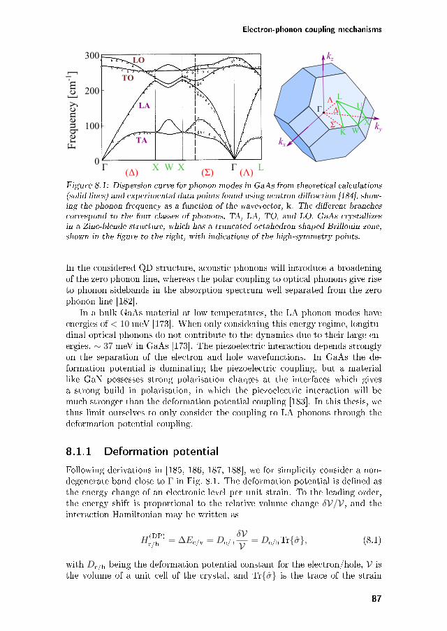
Electron-phonon coupling mechanisms
Fre
quen
cy [
cm-1
]
XX(Δ)Γ Γ(Σ) L(Λ)W
LO
TO
LA
TA
0
100
200
300
LU
XWK
Δ
Σ
Λ
kx
ky
kz
Γ
Figure 8.1: Dispersion curve for phonon modes in GaAs from theoretical calculations(solid lines) and experimental data points found using neutron diffraction [184], show-ing the phonon frequency as a function of the wavevector, k. The different branchescorrespond to the four classes of phonons, TA, LA, TO, and LO. GaAs crystallizesin a Zinc-blende structure, which has a truncated octahedron shaped Brillouin zone,shown in the figure to the right, with indications of the high-symmetry points.
In the considered QD structure, acoustic phonons will introduce a broadeningof the zero phonon line, whereas the polar coupling to optical phonons give riseto phonon sidebands in the absorption spectrum well separated from the zerophonon line [182].
In a bulk GaAs material at low temperatures, the LA phonon modes haveenergies of < 10 meV [173]. When only considering this energy regime, longitu-dinal optical phonons do not contribute to the dynamics due to their large en-ergies, ∼ 37 meV in GaAs [173]. The piezoelectric interaction depends stronglyon the separation of the electron and hole wavefunctions. In GaAs the de-formation potential is dominating the piezoelectric coupling, but a materiallike GaN possesses strong polarisation charges at the interfaces which givesa strong build in polarisation, in which the piezoelectric interaction will bemuch stronger than the deformation potential coupling [183]. In this thesis, wethus limit ourselves to only consider the coupling to LA phonons through thedeformation potential coupling.
8.1.1 Deformation potential
Following derivations in [185, 186, 187, 188], we for simplicity consider a non-degenerate band close to Γ in Fig. 8.1. The deformation potential is defined asthe energy change of an electronic level per unit strain. To the leading order,the energy shift is proportional to the relative volume change 𝛿𝒱/𝒱, and theinteraction Hamiltonian may be written as
𝐻(DP)e/h = ∆𝐸c/v = 𝐷e/h
𝛿𝒱𝒱
= 𝐷e/hTr, (8.1)
with 𝐷e/h being the deformation potential constant for the electron/hole, 𝒱 isthe volume of a unit cell of the crystal, and Tr is the trace of the strain
87
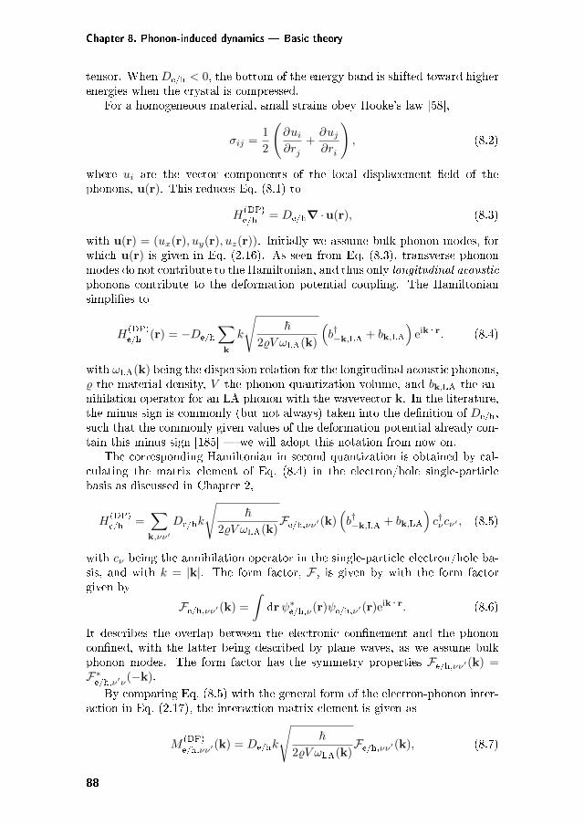
Chapter 8. Phonon-induced dynamics — Basic theory
tensor. When 𝐷e/h < 0, the bottom of the energy band is shifted toward higherenergies when the crystal is compressed.
For a homogeneous material, small strains obey Hooke’s law [58],
𝜎𝑖𝑗 =1
2
(𝜕𝑢𝑖𝜕𝑟𝑗
+𝜕𝑢𝑗𝜕𝑟𝑖
), (8.2)
where 𝑢𝑖 are the vector components of the local displacement field of thephonons, u(r). This reduces Eq. (8.1) to
𝐻(DP)e/h = 𝐷e/h∇ ·u(r), (8.3)
with u(r) = (𝑢𝑥(r), 𝑢𝑦(r), 𝑢𝑧(r)). Initially we assume bulk phonon modes, forwhich u(r) is given in Eq. (2.16). As seen from Eq. (8.3), transverse phononmodes do not contribute to the Hamiltonian, and thus only longitudinal acousticphonons contribute to the deformation potential coupling. The Hamiltoniansimplifies to
𝐻(DP)e/h (r) = −𝐷e/h
∑k
𝑘
√~
2𝜚𝑉 𝜔LA(k)
(𝑏†−k,LA + 𝑏k,LA
)eik · r. (8.4)
with 𝜔LA(k) being the dispersion relation for the longitudinal acoustic phonons,𝜚 the material density, 𝑉 the phonon quantization volume, and 𝑏k,LA the an-nihilation operator for an LA phonon with the wavevector k. In the literature,the minus sign is commonly (but not always) taken into the definition of 𝐷e/h,such that the commonly given values of the deformation potential already con-tain this minus sign [185] — we will adopt this notation from now on.
The corresponding Hamiltonian in second quantization is obtained by cal-culating the matrix element of Eq. (8.4) in the electron/hole single-particlebasis as discussed in Chapter 2,
𝐻(DP)e/h =
∑k,𝜈𝜈′
𝐷e/h𝑘
√~
2𝜚𝑉 𝜔LA(k)ℱe/h,𝜈𝜈′(k)
(𝑏†−k,LA + 𝑏k,LA
)𝑐†𝜈𝑐𝜈′ , (8.5)
with 𝑐𝜈 being the annihilation operator in the single-particle electron/hole ba-sis, and with 𝑘 = |k|. The form factor, ℱ , is given by with the form factorgiven by
ℱe/h,𝜈𝜈′(k) =
∫dr𝜓*
e/h,𝜈(r)𝜓e/h,𝜈′(r)eik · r. (8.6)
It describes the overlap between the electronic confinement and the phononconfined, with the latter being described by plane waves, as we assume bulkphonon modes. The form factor has the symmetry properties ℱe/h,𝜈𝜈′(k) =ℱ*e/h,𝜈′𝜈
(−k).
By comparing Eq. (8.5) with the general form of the electron-phonon inter-action in Eq. (2.17), the interaction matrix element is given as
𝑀(DP)
e/h,𝜈𝜈′(k) = 𝐷e/h𝑘
√~
2𝜚𝑉 𝜔LA(k)ℱe/h,𝜈𝜈′(k), (8.7)
88
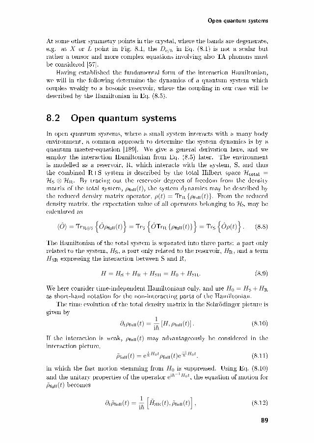
Open quantum systems
At some other symmetry points in the crystal, where the bands are degenerate,e.g. at 𝑋 or 𝐿 point in Fig. 8.1, the 𝐷e/h in Eq. (8.1) is not a scalar butrather a tensor and more complex equations involving also TA phonons mustbe considered [57].
Having established the fundamental form of the interaction Hamiltonian,we will in the following determine the dynamics of a quantum system whichcouples weakly to a bosonic reservoir, where the coupling in our case will bedescribed by the Hamiltonian in Eq. (8.5).
8.2 Open quantum systems
In open quantum systems, where a small system interacts with a many-bodyenvironment, a common approach to determine the system dynamics is by aquantum master-equation [189]. We give a general derivation here, and weemploy the interaction Hamiltonian from Eq. (8.5) later. The environmentis modelled as a reservoir, R, which interacts with the system, S, and thusthe combined R+S system is described by the total Hilbert space ℋtotal =ℋS ⊗ ℋR. By tracing out the reservoir degrees of freedom from the densitymatrix of the total system, 𝜌full(𝑡), the system dynamics may be described bythe reduced density matrix operator, 𝜌(𝑡) = TrR 𝜌full(𝑡). From the reduceddensity matrix, the expectation value of all operators belonging to ℋS may becalculated as
⟨⟩ = TrR⊕S
𝜌full(𝑡)
= TrS
TrR 𝜌full(𝑡)
= TrS
𝜌(𝑡)
. (8.8)
The Hamiltonian of the total system is separated into three parts: a part onlyrelated to the system, 𝐻S, a part only related to the reservoir, 𝐻R, and a term𝐻SR expressing the interaction between S and R,
𝐻 = 𝐻S +𝐻R +𝐻SR = 𝐻0 +𝐻SR. (8.9)
We here consider time-independent Hamiltonians only, and use 𝐻0 = 𝐻S +𝐻R
as short-hand notation for the non-interacting parts of the Hamiltonian.The time evolution of the total density matrix in the Schrödinger picture is
given by
𝜕𝑡𝜌full(𝑡) =1
i~[𝐻, 𝜌full(𝑡)] . (8.10)
If the interaction is weak, 𝜌full(𝑡) may advantageously be considered in theinteraction picture,
𝜌full(𝑡) = ei~𝐻0𝑡𝜌full(𝑡)e
−i~ 𝐻0𝑡. (8.11)
in which the fast motion stemming from 𝐻0 is suppressed. Using Eq. (8.10)and the unitary properties of the operator ei~
−1𝐻0𝑡, the equation of motion for𝜌full(𝑡) becomes
𝜕𝑡𝜌full(𝑡) =1
i~
[SR(𝑡), 𝜌full(𝑡)
], (8.12)
89
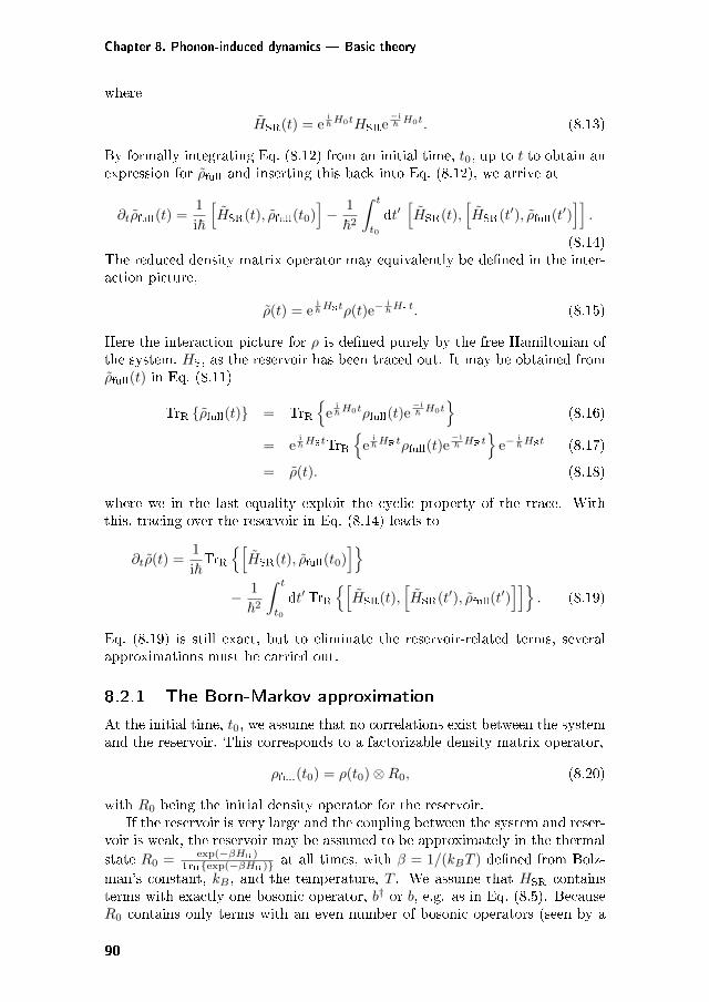
Chapter 8. Phonon-induced dynamics — Basic theory
where
SR(𝑡) = ei~𝐻0𝑡𝐻SRe
−i~ 𝐻0𝑡. (8.13)
By formally integrating Eq. (8.12) from an initial time, 𝑡0, up to 𝑡 to obtain anexpression for 𝜌full and inserting this back into Eq. (8.12), we arrive at
𝜕𝑡𝜌full(𝑡) =1
i~
[SR(𝑡), 𝜌full(𝑡0)
]− 1
~2
∫ 𝑡
𝑡0
d𝑡′[SR(𝑡),
[SR(𝑡′), 𝜌full(𝑡
′)]].
(8.14)The reduced density matrix operator may equivalently be defined in the inter-action picture,
𝜌(𝑡) = ei~𝐻S𝑡𝜌(𝑡)e−
i~𝐻S𝑡. (8.15)
Here the interaction picture for 𝜌 is defined purely by the free Hamiltonian ofthe system, 𝐻S, as the reservoir has been traced out. It may be obtained from𝜌full(𝑡) in Eq. (8.11)
TrR 𝜌full(𝑡) = TrR
ei~𝐻0𝑡𝜌full(𝑡)e
−i~ 𝐻0𝑡
(8.16)
= ei~𝐻S𝑡TrR
e
i~𝐻R𝑡𝜌full(𝑡)e
−i~ 𝐻R𝑡
e−
i~𝐻S𝑡 (8.17)
= 𝜌(𝑡). (8.18)
where we in the last equality exploit the cyclic property of the trace. Withthis, tracing over the reservoir in Eq. (8.14) leads to
𝜕𝑡𝜌(𝑡) =1
i~TrR
[SR(𝑡), 𝜌full(𝑡0)
]− 1
~2
∫ 𝑡
𝑡0
d𝑡′TrR[SR(𝑡),
[SR(𝑡′), 𝜌full(𝑡
′)]]
. (8.19)
Eq. (8.19) is still exact, but to eliminate the reservoir-related terms, severalapproximations must be carried out.
8.2.1 The Born-Markov approximation
At the initial time, 𝑡0, we assume that no correlations exist between the systemand the reservoir. This corresponds to a factorizable density matrix operator,
𝜌full(𝑡0) = 𝜌(𝑡0) ⊗𝑅0, (8.20)
with 𝑅0 being the initial density operator for the reservoir.If the reservoir is very large and the coupling between the system and reser-
voir is weak, the reservoir may be assumed to be approximately in the thermalstate 𝑅0 = exp(−𝛽𝐻R)
TrRexp(−𝛽𝐻R) at all times, with 𝛽 = 1/(𝑘𝐵𝑇 ) defined from Bolz-man’s constant, 𝑘𝐵 , and the temperature, 𝑇 . We assume that 𝐻SR containsterms with exactly one bosonic operator, 𝑏† or 𝑏, e.g. as in Eq. (8.5). Because𝑅0 contains only terms with an even number of bosonic operators (seen by a
90
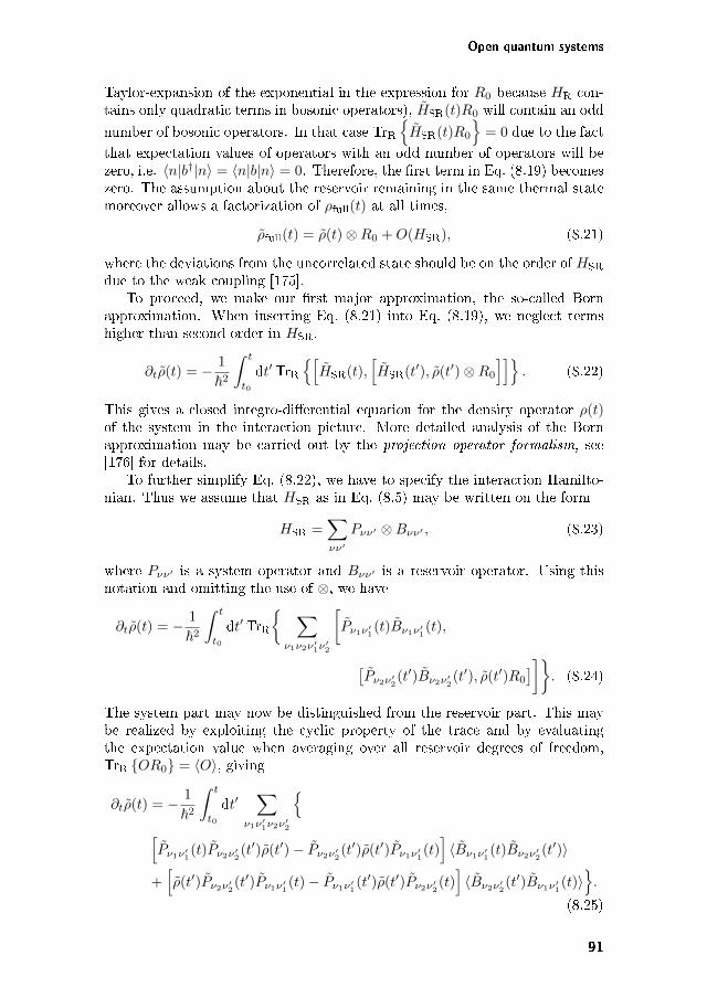
Open quantum systems
Taylor-expansion of the exponential in the expression for 𝑅0 because 𝐻R con-tains only quadratic terms in bosonic operators), SR(𝑡)𝑅0 will contain an odd
number of bosonic operators. In that case TrRSR(𝑡)𝑅0
= 0 due to the fact
that expectation values of operators with an odd number of operators will bezero, i.e. ⟨𝑛|𝑏†|𝑛⟩ = ⟨𝑛|𝑏|𝑛⟩ = 0. Therefore, the first term in Eq. (8.19) becomeszero. The assumption about the reservoir remaining in the same thermal statemoreover allows a factorization of 𝜌full(𝑡) at all times,
𝜌full(𝑡) = 𝜌(𝑡) ⊗𝑅0 +𝑂(𝐻SR), (8.21)
where the deviations from the uncorrelated state should be on the order of 𝐻SR
due to the weak coupling [175].To proceed, we make our first major approximation, the so-called Born
approximation. When inserting Eq. (8.21) into Eq. (8.19), we neglect termshigher than second order in 𝐻SR,
𝜕𝑡𝜌(𝑡) = − 1
~2
∫ 𝑡
𝑡0
d𝑡′ TrR[SR(𝑡),
[SR(𝑡′), 𝜌(𝑡′) ⊗𝑅0
]]. (8.22)
This gives a closed integro-differential equation for the density operator 𝜌(𝑡)of the system in the interaction picture. More detailed analysis of the Bornapproximation may be carried out by the projection operator formalism, see[176] for details.
To further simplify Eq. (8.22), we have to specify the interaction Hamilto-nian. Thus we assume that 𝐻SR as in Eq. (8.5) may be written on the form
𝐻SR =∑𝜈𝜈′
𝑃𝜈𝜈′ ⊗𝐵𝜈𝜈′ , (8.23)
where 𝑃𝜈𝜈′ is a system operator and 𝐵𝜈𝜈′ is a reservoir operator. Using thisnotation and omitting the use of ⊗, we have
𝜕𝑡𝜌(𝑡) = − 1
~2
∫ 𝑡
𝑡0
d𝑡′TrR
∑𝜈1𝜈2𝜈′
1𝜈′2
[𝑃𝜈1𝜈′
1(𝑡)𝜈1𝜈′
1(𝑡),
[𝑃𝜈2𝜈′
2(𝑡′)𝜈2𝜈′
2(𝑡′), 𝜌(𝑡′)𝑅0
]]. (8.24)
The system part may now be distinguished from the reservoir part. This maybe realized by exploiting the cyclic property of the trace and by evaluatingthe expectation value when averaging over all reservoir degrees of freedom,TrR 𝑂𝑅0 = ⟨𝑂⟩, giving
𝜕𝑡𝜌(𝑡) = − 1
~2
∫ 𝑡
𝑡0
d𝑡′∑
𝜈1𝜈′1𝜈2𝜈′
2
[𝑃𝜈1𝜈′
1(𝑡)𝑃𝜈2𝜈′
2(𝑡′)𝜌(𝑡′) − 𝑃𝜈2𝜈′
2(𝑡′)𝜌(𝑡′)𝑃𝜈1𝜈′
1(𝑡)]⟨𝜈1𝜈′
1(𝑡)𝜈2𝜈′
2(𝑡′)⟩
+[𝜌(𝑡′)𝑃𝜈2𝜈′
2(𝑡′)𝑃𝜈1𝜈′
1(𝑡) − 𝑃𝜈1𝜈′
1(𝑡′)𝜌(𝑡′)𝑃𝜈2𝜈′
2(𝑡)]⟨𝜈2𝜈′
2(𝑡′)𝜈1𝜈′
1(𝑡)⟩.
(8.25)
91
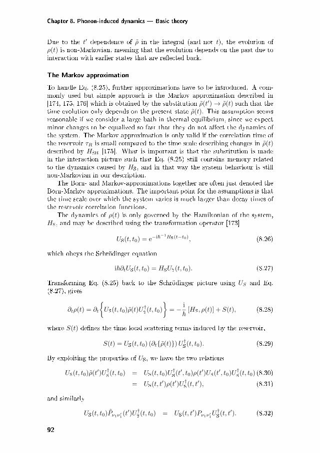
Chapter 8. Phonon-induced dynamics — Basic theory
Due to the 𝑡′ dependence of 𝜌 in the integral (and not 𝑡), the evolution of𝜌(𝑡) is non-Markovian, meaning that the evolution depends on the past due tointeraction with earlier states that are reflected back.
The Markov approximation
To handle Eq. (8.25), further approximations have to be introduced. A com-monly used but simple approach is the Markov approximation described in[174, 175, 176] which is obtained by the substitution 𝜌(𝑡′) → 𝜌(𝑡) such that thetime evolution only depends on the present state 𝜌(𝑡). This assumption seemsreasonable if we consider a large bath in thermal equilibrium, since we expectminor changes to be equalized so fast that they do not affect the dynamics ofthe system. The Markov approximation is only valid if the correlation time ofthe reservoir 𝜏𝑅 is small compared to the time scale describing changes in 𝜌(𝑡)described by 𝐻SR [175]. What is important is that the substitution is madein the interaction picture such that Eq. (8.25) still contains memory relatedto the dynamics caused by 𝐻S, and in that way the system behaviour is stillnon-Markovian in our description.
The Born- and Markov-approximations together are often just denoted theBorn-Markov approximations. The important point for the assumptions is thatthe time scale over which the system varies is much larger than decay times ofthe reservoir correlation functions.
The dynamics of 𝜌(𝑡) is only governed by the Hamiltonian of the system,𝐻S, and may be described using the transformation operator [173]
𝑈S(𝑡, 𝑡0) = e−i~−1𝐻S(𝑡−𝑡0), (8.26)
which obeys the Schrödinger equation
i~𝜕𝑡𝑈S(𝑡, 𝑡0) = 𝐻S𝑈S(𝑡, 𝑡0). (8.27)
Transforming Eq. (8.25) back to the Schrödinger picture using 𝑈𝑆 and Eq.(8.27), gives
𝜕𝑡𝜌(𝑡) = 𝜕𝑡
𝑈S(𝑡, 𝑡0)𝜌(𝑡)𝑈†
S(𝑡, 𝑡0)
= − i
~[𝐻S, 𝜌(𝑡)] + 𝑆(𝑡), (8.28)
where 𝑆(𝑡) defines the time-local scattering terms induced by the reservoir,
𝑆(𝑡) = 𝑈S(𝑡, 𝑡0) (𝜕𝑡𝜌(𝑡))𝑈†S(𝑡, 𝑡0). (8.29)
By exploiting the properties of 𝑈S, we have the two relations
𝑈S(𝑡, 𝑡0)𝜌(𝑡′)𝑈†S(𝑡, 𝑡0) = 𝑈S(𝑡, 𝑡0)𝑈†
S(𝑡′, 𝑡0)𝜌(𝑡′)𝑈S(𝑡′, 𝑡0)𝑈†S(𝑡, 𝑡0) (8.30)
= 𝑈S(𝑡, 𝑡′)𝜌(𝑡′)𝑈†S(𝑡, 𝑡′), (8.31)
and similarly
𝑈S(𝑡, 𝑡0)𝑃𝜈1𝜈′1(𝑡′)𝑈†
S(𝑡, 𝑡0) = 𝑈S(𝑡, 𝑡′)𝑃𝜈1𝜈′1𝑈†S(𝑡, 𝑡′). (8.32)
92
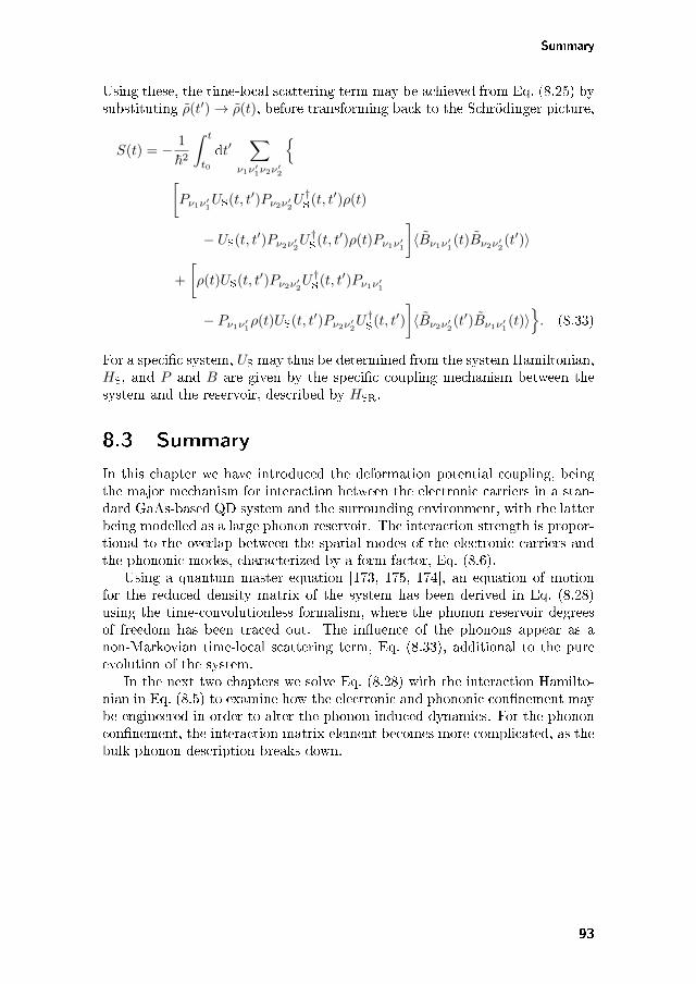
Summary
Using these, the time-local scattering term may be achieved from Eq. (8.25) bysubstituting 𝜌(𝑡′) → 𝜌(𝑡), before transforming back to the Schrödinger picture,
𝑆(𝑡) = − 1
~2
∫ 𝑡
𝑡0
d𝑡′∑
𝜈1𝜈′1𝜈2𝜈′
2
[𝑃𝜈1𝜈′
1𝑈S(𝑡, 𝑡′)𝑃𝜈2𝜈′
2𝑈†S(𝑡, 𝑡′)𝜌(𝑡)
− 𝑈S(𝑡, 𝑡′)𝑃𝜈2𝜈′2𝑈†S(𝑡, 𝑡′)𝜌(𝑡)𝑃𝜈1𝜈′
1
]⟨𝜈1𝜈′
1(𝑡)𝜈2𝜈′
2(𝑡′)⟩
+
[𝜌(𝑡)𝑈S(𝑡, 𝑡′)𝑃𝜈2𝜈′
2𝑈†S(𝑡, 𝑡′)𝑃𝜈1𝜈′
1
− 𝑃𝜈1𝜈′1𝜌(𝑡)𝑈S(𝑡, 𝑡′)𝑃𝜈2𝜈′
2𝑈†S(𝑡, 𝑡′)
]⟨𝜈2𝜈′
2(𝑡′)𝜈1𝜈′
1(𝑡)⟩. (8.33)
For a specific system, 𝑈S may thus be determined from the system Hamiltonian,𝐻S, and 𝑃 and 𝐵 are given by the specific coupling mechanism between thesystem and the reservoir, described by 𝐻SR.
8.3 Summary
In this chapter we have introduced the deformation potential coupling, beingthe major mechanism for interaction between the electronic carriers in a stan-dard GaAs-based QD system and the surrounding environment, with the latterbeing modelled as a large phonon reservoir. The interaction strength is propor-tional to the overlap between the spatial modes of the electronic carriers andthe phononic modes, characterized by a form factor, Eq. (8.6).
Using a quantum master equation [173, 175, 174], an equation of motionfor the reduced density matrix of the system has been derived in Eq. (8.28)using the time-convolutionless formalism, where the phonon reservoir degreesof freedom has been traced out. The influence of the phonons appear as anon-Markovian time-local scattering term, Eq. (8.33), additional to the pureevolution of the system.
In the next two chapters we solve Eq. (8.28) with the interaction Hamilto-nian in Eq. (8.5) to examine how the electronic and phononic confinement maybe engineered in order to alter the phonon-induced dynamics. For the phononconfinement, the interaction matrix element becomes more complicated, as thebulk phonon description breaks down.
93

Chapter 9
Phonon-induced dynamics
— The electronic
confinement
In this chapter we investigate the role of carrier confinement on phonon scat-tering in a semiconductor quantum dot (QD). We employ the comprehensivetheoretical model described in Chapter 8 that takes into account the non-Markovian nature of the phonon reservoir [48], thus avoiding the standardapproach of describing phonon-induced decoherence by a pure dephasing rate[190, 191]. Surprisingly, we find that deformation potential scattering may becompletely quenched under certain conditions, depending on the degree of con-finement of the involved electronic states. The effect is investigated in detailfor two cases.
Firstly in Section 9.1, we consider photoluminescence spectroscopy of a sin-gle QD and find that the luminescence is suppressed at certain detunings due toa quenching of phonon scattering. Approximate analytic results show that theeffect originates from the difference in the spatial confinement of electrons andholes, usually neglected in theoretical treatments. Secondly in Section 9.2, wefind that quenching of phonon scattering strongly affects pure dephasing in cou-pled QD-cavity systems. Expanding the description to realistic QD structures,which are analyzed numerically, conditions for reducing phonon scattering areestablished. Lastly in Section 9.3, the phonon model is applied to an exper-imental measurement of the decay rate of a QD inside a L3 photonic crystalcavity, by which we are able to map out the effective phonon density of states,which to our knowledge has not been demonstrated before [172].
Other approaches towards controlling the degree of phonon scattering usephononic bandgap structures for suppressing vibrational modes [192] or consid-ers QDs near surfaces [193], which will be discussed in the next chapter. Struc-tures with simultaneous photonic and phononic bandgaps have been discussedtheoretically [194] and experimentally realized [195] with phononic bandgapsin the GHz-regime. In cavity QED, the most relevant phonons belong to the
95
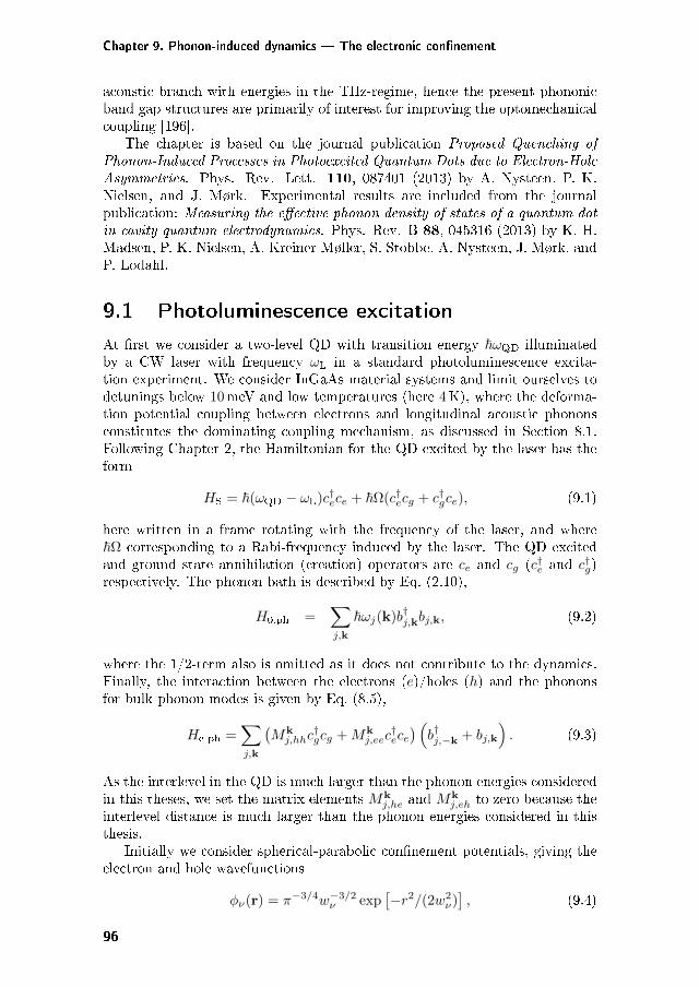
Chapter 9. Phonon-induced dynamics — The electronic confinement
acoustic branch with energies in the THz-regime, hence the present phononicband gap structures are primarily of interest for improving the optomechanicalcoupling [196].
The chapter is based on the journal publication Proposed Quenching ofPhonon-Induced Processes in Photoexcited Quantum Dots due to Electron-HoleAsymmetries. Phys. Rev. Lett. 110, 087401 (2013) by A. Nysteen, P. K.Nielsen, and J. Mørk. Experimental results are included from the journalpublication: Measuring the effective phonon density of states of a quantum dotin cavity quantum electrodynamics. Phys. Rev. B 88, 045316 (2013) by K. H.Madsen, P. K. Nielsen, A. Kreiner-Møller, S. Stobbe, A. Nysteen, J. Mørk, andP. Lodahl.
9.1 Photoluminescence excitation
At first we consider a two-level QD with transition energy ~𝜔QD illuminatedby a CW laser with frequency 𝜔L in a standard photoluminescence excita-tion experiment. We consider InGaAs material systems and limit ourselves todetunings below 10meV and low temperatures (here 4K), where the deforma-tion potential coupling between electrons and longitudinal acoustic phononsconstitutes the dominating coupling mechanism, as discussed in Section 8.1.Following Chapter 2, the Hamiltonian for the QD excited by the laser has theform
𝐻S = ~(𝜔QD − 𝜔L)𝑐†𝑒𝑐𝑒 + ~Ω(𝑐†𝑒𝑐𝑔 + 𝑐†𝑔𝑐𝑒), (9.1)
here written in a frame rotating with the frequency of the laser, and where~Ω corresponding to a Rabi-frequency induced by the laser. The QD excitedand ground state annihilation (creation) operators are 𝑐𝑒 and 𝑐𝑔 (𝑐†𝑒 and 𝑐†𝑔)respectively. The phonon bath is described by Eq. (2.10),
𝐻0,ph =∑𝑗,k
~𝜔𝑗(k)𝑏†𝑗,k𝑏𝑗,k, (9.2)
where the 1/2-term also is omitted as it does not contribute to the dynamics.Finally, the interaction between the electrons (𝑒)/holes (ℎ) and the phononsfor bulk phonon modes is given by Eq. (8.5),
𝐻e-ph =∑𝑗,k
(𝑀k
𝑗,ℎℎ𝑐†𝑔𝑐𝑔 +𝑀k
𝑗,𝑒𝑒𝑐†𝑒𝑐𝑒) (𝑏†𝑗,−k + 𝑏𝑗,k
). (9.3)
As the interlevel in the QD is much larger than the phonon energies consideredin this theses, we set the matrix elements 𝑀k
𝑗,ℎ𝑒 and 𝑀k𝑗,𝑒ℎ to zero because the
interlevel distance is much larger than the phonon energies considered in thisthesis.
Initially we consider spherical-parabolic confinement potentials, giving theelectron and hole wavefunctions
𝜑𝜈(r) = 𝜋−3/4𝑤−3/2𝜈 exp
[−𝑟2/(2𝑤2
𝜈)], (9.4)
96
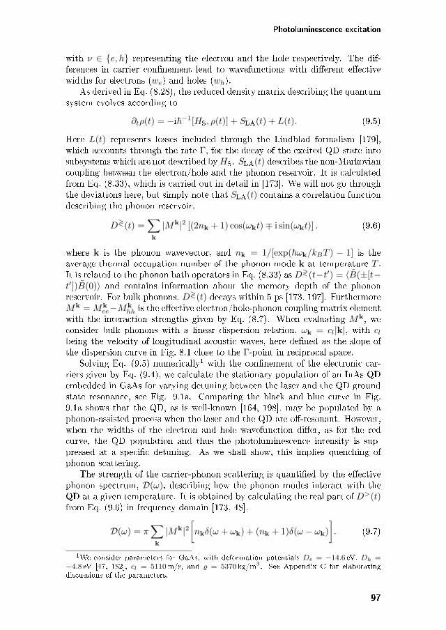
Photoluminescence excitation
with 𝜈 ∈ 𝑒, ℎ representing the electron and the hole respectively. The dif-ferences in carrier confinement lead to wavefunctions with different effectivewidths for electrons (𝑤𝑒) and holes (𝑤ℎ).
As derived in Eq. (8.28), the reduced density matrix describing the quantumsystem evolves according to
𝜕𝑡𝜌(𝑡) = −i~−1[𝐻S, 𝜌(𝑡)] + 𝑆LA(𝑡) + 𝐿(𝑡). (9.5)
Here 𝐿(𝑡) represents losses included through the Lindblad formalism [179],which accounts through the rate Γ, for the decay of the excited QD state intosubsystems which are not described by𝐻S. 𝑆LA(𝑡) describes the non-Markoviancoupling between the electron/hole and the phonon reservoir. It is calculatedfrom Eq. (8.33), which is carried out in detail in [173]. We will not go throughthe deviations here, but simply note that 𝑆LA(𝑡) contains a correlation functiondescribing the phonon reservoir,
𝐷≷(𝑡) =∑k
|𝑀k|2 [(2𝑛k + 1) cos(𝜔k𝑡) ∓ i sin(𝜔k𝑡)] . (9.6)
where k is the phonon wavevector, and 𝑛k = 1/[exp(~𝜔k/𝑘𝐵𝑇 ) − 1] is theaverage thermal occupation number of the phonon mode k at temperature 𝑇 .It is related to the phonon bath operators in Eq. (8.33) as 𝐷≷(𝑡−𝑡′) = ⟨(±[𝑡−𝑡′])(0)⟩ and contains information about the memory depth of the phononreservoir. For bulk phonons, 𝐷≷(𝑡) decays within 5 ps [173, 197]. Furthermore𝑀k = 𝑀k
𝑒𝑒−𝑀kℎℎ is the effective electron/hole-phonon coupling matrix element
with the interaction strengths given by Eq. (8.7). When evaluating 𝑀k, weconsider bulk phonons with a linear dispersion relation, 𝜔k = 𝑐𝑙|k|, with 𝑐𝑙being the velocity of longitudinal acoustic waves, here defined as the slope ofthe dispersion curve in Fig. 8.1 close to the Γ-point in reciprocal space.
Solving Eq. (9.5) numerically1 with the confinement of the electronic car-riers given by Eq. (9.4), we calculate the stationary population of an InAs QDembedded in GaAs for varying detuning between the laser and the QD groundstate resonance, see Fig. 9.1a. Comparing the black and blue curve in Fig.9.1a shows that the QD, as is well-known [164, 198], may be populated by aphonon-assisted process when the laser and the QD are off-resonant. However,when the widths of the electron and hole wavefunction differ, as for the redcurve, the QD population and thus the photoluminescence intensity is sup-pressed at a specific detuning. As we shall show, this implies quenching ofphonon scattering.
The strength of the carrier-phonon scattering is quantified by the effectivephonon spectrum, 𝒟(𝜔), describing how the phonon modes interact with theQD at a given temperature. It is obtained by calculating the real part of 𝐷>(𝑡)from Eq. (9.6) in frequency domain [173, 48],
𝒟(𝜔) = 𝜋∑k
|𝑀k|2[𝑛k𝛿(𝜔 + 𝜔k) + (𝑛k + 1)𝛿(𝜔 − 𝜔k)
]. (9.7)
1We consider parameters for GaAs, with deformation potentials 𝐷𝑒 = −14.6 eV, 𝐷ℎ =−4.8 eV [47, 182], 𝑐𝑙 = 5110m/s, and 𝜚 = 5370 kg/m3. See Appendix C for elaboratingdiscussions of the parameters.
97
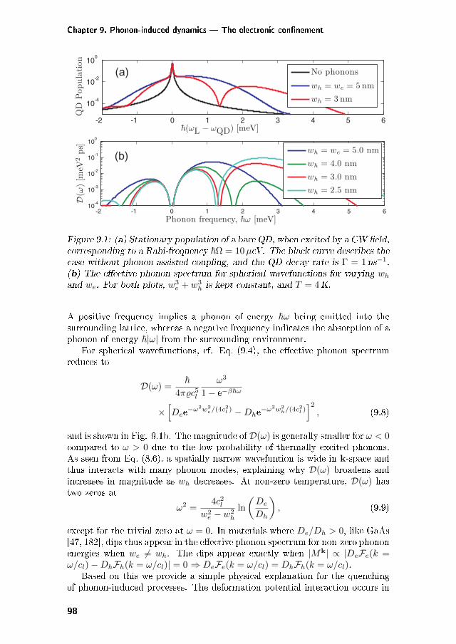
Chapter 9. Phonon-induced dynamics — The electronic confinement
(b)
(a)
Figure 9.1: (a) Stationary population of a bare QD, when excited by a CW field,corresponding to a Rabi-frequency ~Ω = 10𝜇eV. The black curve describes thecase without phonon-assisted coupling, and the QD decay rate is Γ = 1ns−1.(b) The effective phonon spectrum for spherical wavefunctions for varying 𝑤ℎ
and 𝑤𝑒. For both plots, 𝑤3𝑒 + 𝑤3
ℎ is kept constant, and 𝑇 = 4K.
A positive frequency implies a phonon of energy ~𝜔 being emitted into thesurrounding lattice, whereas a negative frequency indicates the absorption of aphonon of energy ~|𝜔| from the surrounding environment.
For spherical wavefunctions, cf. Eq. (9.4), the effective phonon spectrumreduces to
𝒟(𝜔) =~
4𝜋𝜚𝑐5𝑙
𝜔3
1 − e−𝛽~𝜔
×[𝐷𝑒e
−𝜔2𝑤2𝑒/(4𝑐
2𝑙 ) −𝐷ℎe
−𝜔2𝑤2ℎ/(4𝑐
2𝑙 )]2, (9.8)
and is shown in Fig. 9.1b. The magnitude of 𝒟(𝜔) is generally smaller for 𝜔 < 0compared to 𝜔 > 0 due to the low probability of thermally excited phonons.As seen from Eq. (8.6), a spatially narrow wavefuntion is wide in k-space andthus interacts with many phonon modes, explaining why 𝒟(𝜔) broadens andincreases in magnitude as 𝑤ℎ decreases. At non-zero temperature, 𝒟(𝜔) hastwo zeros at
𝜔2 =4𝑐2𝑙
𝑤2𝑒 − 𝑤2
ℎ
ln
(𝐷𝑒
𝐷ℎ
), (9.9)
except for the trivial zero at 𝜔 = 0. In materials where 𝐷𝑒/𝐷ℎ > 0, like GaAs[47, 182], dips thus appear in the effective phonon spectrum for non-zero phononenergies when 𝑤𝑒 = 𝑤ℎ. The dips appear exactly when |𝑀k| ∝ |𝐷𝑒ℱ𝑒(𝑘 =𝜔/𝑐𝑙) −𝐷ℎℱℎ(𝑘 = 𝜔/𝑐𝑙)| = 0 ⇒ 𝐷𝑒ℱ𝑒(𝑘 = 𝜔/𝑐𝑙) = 𝐷ℎℱℎ(𝑘 = 𝜔/𝑐𝑙).
Based on this we provide a simple physical explanation for the quenchingof phonon-induced processes. The deformation potential interaction occurs in
98
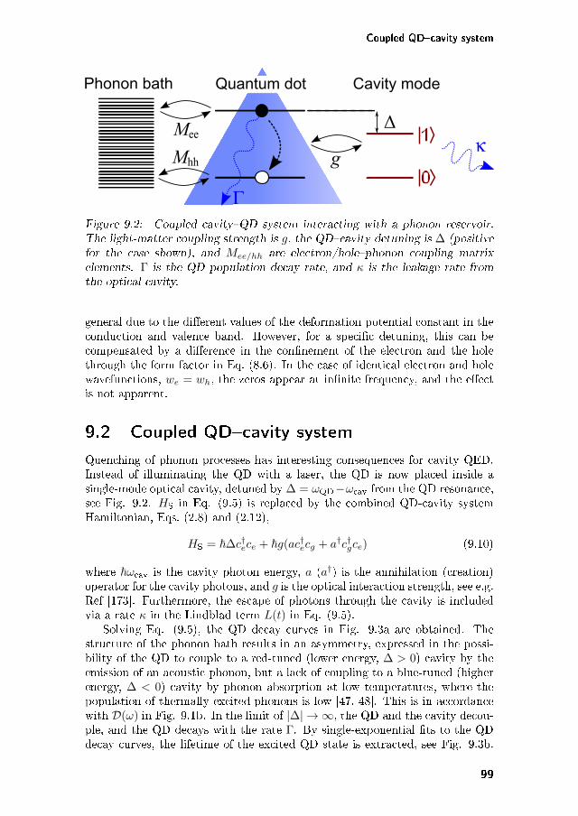
Coupled QD–cavity system
Cavity modeQuantum dotPhonon bath
Meek
G
Δ1
gMhh
0
Figure 9.2: Coupled cavity–QD system interacting with a phonon reservoir.The light-matter coupling strength is 𝑔, the QD–cavity detuning is ∆ (positivefor the case shown), and 𝑀𝑒𝑒/ℎℎ are electron/hole–phonon coupling matrixelements. Γ is the QD population decay rate, and 𝜅 is the leakage rate fromthe optical cavity.
general due to the different values of the deformation potential constant in theconduction and valence band. However, for a specific detuning, this can becompensated by a difference in the confinement of the electron and the holethrough the form factor in Eq. (8.6). In the case of identical electron and holewavefunctions, 𝑤𝑒 = 𝑤ℎ, the zeros appear at infinite frequency, and the effectis not apparent.
9.2 Coupled QD–cavity system
Quenching of phonon processes has interesting consequences for cavity QED.Instead of illuminating the QD with a laser, the QD is now placed inside asingle-mode optical cavity, detuned by ∆ = 𝜔QD−𝜔cav from the QD resonance,see Fig. 9.2. 𝐻S in Eq. (9.5) is replaced by the combined QD-cavity systemHamiltonian, Eqs. (2.8) and (2.12),
𝐻S = ~∆𝑐†𝑒𝑐𝑒 + ~𝑔(𝑎𝑐†𝑒𝑐𝑔 + 𝑎†𝑐†𝑔𝑐𝑒) (9.10)
where ~𝜔cav is the cavity photon energy, 𝑎 (𝑎†) is the annihilation (creation)operator for the cavity photons, and 𝑔 is the optical interaction strength, see e.g.Ref [173]. Furthermore, the escape of photons through the cavity is includedvia a rate 𝜅 in the Lindblad term 𝐿(𝑡) in Eq. (9.5).
Solving Eq. (9.5), the QD decay curves in Fig. 9.3a are obtained. Thestructure of the phonon bath results in an asymmetry, expressed in the possi-bility of the QD to couple to a red-tuned (lower energy, ∆ > 0) cavity by theemission of an acoustic phonon, but a lack of coupling to a blue-tuned (higherenergy, ∆ < 0) cavity by phonon absorption at low temperatures, where thepopulation of thermally excited phonons is low [47, 48]. This is in accordancewith 𝒟(𝜔) in Fig. 9.1b. In the limit of |∆| → ∞, the QD and the cavity decou-ple, and the QD decays with the rate Γ. By single-exponential fits to the QDdecay curves, the lifetime of the excited QD state is extracted, see Fig. 9.3b.
99
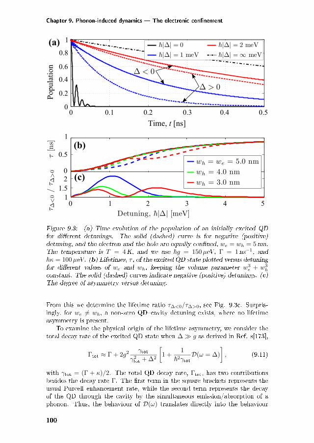
Chapter 9. Phonon-induced dynamics — The electronic confinement
Time, t [ns]
Pop
ulat
ion
0 0.1 0.2 0.3 0.4 0.5
1
0.8
0.6
0.4
0.2
0
1
0.5
02
1.51
0 1 2 3 4 5
(c)
(a)
(b)
Figure 9.3: (a) Time evolution of the population of an initially excited QDfor different detunings. The solid (dashed) curve is for negative (positive)detuning, and the electron and the hole are equally confined, 𝑤𝑒 = 𝑤ℎ = 5nm.The temperature is 𝑇 = 4K, and we use ~𝑔 = 150𝜇eV, Γ = 1 ns−1, and~𝜅 = 100𝜇eV. (b) Lifetimes, 𝜏 , of the excited QD state plotted versus detuningfor different values of 𝑤𝑒 and 𝑤ℎ, keeping the volume parameter 𝑤3
𝑒 + 𝑤3ℎ
constant. The solid (dashed) curves indicate negative (positive) detunings. (c)The degree of asymmetry versus detuning.
From this we determine the lifetime ratio 𝜏Δ<0/𝜏Δ>0, see Fig. 9.3c. Surpris-ingly, for 𝑤𝑒 = 𝑤ℎ, a non-zero QD–cavity detuning exists, where no lifetimeasymmetry is present.
To examine the physical origin of the lifetime asymmetry, we consider thetotal decay rate of the excited QD state when ∆ ≫ 𝑔 as derived in Ref. s[173],
Γtot ≈ Γ + 2𝑔2𝛾tot
𝛾2tot + ∆2
[1 +
1
~2𝛾tot𝒟(𝜔 = ∆)
], (9.11)
with 𝛾tot = (Γ + 𝜅)/2. The total QD decay rate, Γtot, has two contributionsbesides the decay rate Γ. The first term in the square brackets represents theusual Purcell enhancement rate, while the second term represents the decayof the QD through the cavity by the simultaneous emission/absorption of aphonon. Thus, the behaviour of 𝒟(𝜔) translates directly into the behaviour
100
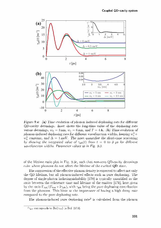
Coupled QD–cavity system
(a)
(b)
0 2 4 6 8
-10
0
10
20
30
40
0
5
10
15
20
25
t [ps]0 2 4 6 8
γ ph(t)
[ns
-1]
γ ph(t)
[ns
-1]
t [ps]
Figure 9.4: (a) Time evolution of phonon-induced dephasing rate for differentQD-cavity detunings. Inset shows the long-time value of the dephasing rateversus detunings, 𝑤ℎ = 3nm, 𝑤𝑒 = 6nm, and 𝑇 = 4K. (b) Time evolution ofphonon-induced dephasing rate for different wavefunction widths, keeping 𝑤3
𝑒 +𝑤3
ℎ constant, and ∆ = 1meV. The inset quantifies the short-time scatteringby showing the integrated value of 𝛾ph(𝑡) from 𝑡 = 0 to 3 ps for differentwavefunction widths. Parameter values as in Fig. 9.3.
of the lifetime ratio plot in Fig. 9.3c, such that non-zero QD-cavity detuningsexist where phonons do not affect the lifetime of the excited QD state.
The suppression of the effective phonon density is expected to affect not onlythe QD lifetime, but all phonon-induced effects such as pure dephasing. Thedegree of single-photon indistinguishability [170] is typically quantified as theratio between the coherence time and lifetime of the emitter [171], here givenby the ratio Γtot/(Γtot +2𝛾ph), with 𝛾ph being the pure dephasing contributionfrom the phonons. This hints at the importance of having a high decay ratecompared to the pure dephasing rate.
The phonon-induced pure dephasing rate2 is calculated from the phonon
2𝛾ph corresponds to Re𝛾12 in Ref. [173].
101
Chapter 9. Phonon-induced dynamics — The electronic confinement
bath correlation function [173], and we find it to be given by
𝛾ph(𝑡) = Re
~−2(1 −𝐾)
∫ 𝑡
0
d𝑡′ 𝒟<(𝑡′)
+~−2𝐾
∫ 𝑡
0
d𝑡′ cos(𝑡′√
∆2 + 4𝑔2)𝒟<(𝑡′)
, (9.12)
where 𝐾 = 4𝜆2+/(1 + 𝜆2+)2 with 𝜆+ = ∆/(2𝑔) +√
∆2/(2𝑔)2 + 1. As seen fromFig. 9.4a, the initial behaviour of 𝛾ph(𝑡) is governed by the bare QD-phononcoupling, whereas the long-time value depends on the cavity detuning. Onthe short time scale, the phonons participate in non-energy conserving virtualprocesses, and the electrons interact with the full phonon spectrum 𝒟(𝜔). Thelong-time value 𝛾ph(𝑡→ ∞), on the other hand, implies a Fourier transform of𝒟(𝑡) and depends only on 𝒟(𝜔 = 0), which is zero, and 𝒟(𝜔 = ±
√∆2 + 4𝑔2),
corresponding to sampling the spectrum at the polaritonic eigenenergies.The phonon-induced dephasing of the QD–cavity system may be reduced by
minimizing the short-time or long-time scattering. The former may be achievedby reducing the overall amplitude of 𝒟(𝜔), as illustrated in the inset of Fig.9.4b for 𝑤ℎ ∼ 3.4 nm, compare with Fig. 9.1b. The reduction of long-timescattering is obtained by using a QD–cavity detuning such that
√∆2 + 4𝑔2
coincides with a dip in 𝒟(𝜔), as seen from the inset in Fig. 9.4a. It turns outthat for the indistinguishability of single photons, the reduction of the overallamplitude is the most important [49]. The coupling to excited shells in the QDthrough virtual phonon interactions induces additional pure dephasing [167].However, for 𝑇 < 10 K this amounts to a weak background, with no qualitativeeffect on our result. Furthermore, for the dot sizes considered here, the nextelectronic energy levels are well-separated compared to the acoustic phononenergies [199], and these levels are neglected.
QD structures realized by epitaxial growth are not spherically symmet-ric [200], and to investigate the quenching for more realistic structures, wemodel truncated conical QD structures by solving the one-band effective massSchrödinger equation using the Finite Element Method (FEM) [201]. Strain-induced effects [200] were not included, but since the strain strongly dependson the QD geometry, material and growth conditions, it may further suppressor enhance phonon scattering, thus presenting another option for engineeringthe basic properties.
The effective phonon spectrum obtained with the FEM wavefunctions isshown in Fig. 9.5a for an InAs QD and wetting layer embedded in a GaAsbarrier3. The overall amplitude of the spectrum is the largest, when the carriersare strongly confined in two directions, i.e. for the tallest dot, compared to theshallow dot where the carriers are only strongly confined in one direction. Theseresults are qualitatively explained by the form factor in Eq. (8.6).
To examine the role of material composition, we consider an In𝑦Ga1−𝑦AsQD, where the amount of gallium in the QD and wetting layer is varied. Increas-
3We use 𝐸𝑔,GaAs = 1.424 eV, 𝐸𝑔,InAs = 0.359 eV, 𝑚*𝑐,GaAs = 0.0665𝑚0, 𝑚*
𝑐,InAs =0.027𝑚0, 𝑚*
𝑣,GaAs = 0.38𝑚0, 𝑚*𝑣,InAs = 0.34𝑚0, and a wetting layer thickness of 0.2 nm
[201, 202].
102
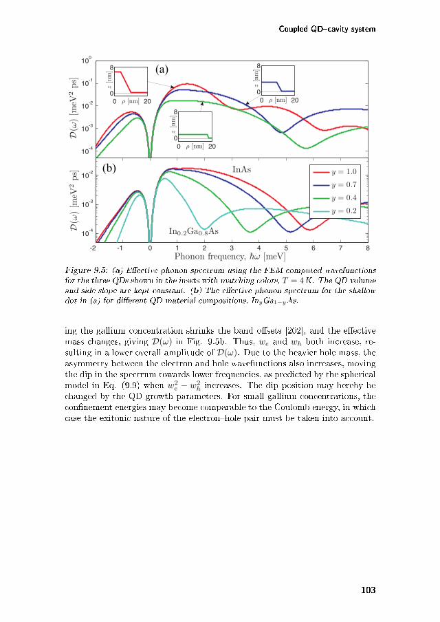
Coupled QD–cavity system
(a)
(b)
Figure 9.5: (a) Effective phonon spectrum using the FEM-computed wavefunctionsfor the three QDs shown in the insets with matching colors, 𝑇 = 4K. The QD volumeand side slope are kept constant. (b) The effective phonon spectrum for the shallowdot in (a) for different QD material compositions, In𝑦Ga1−𝑦As.
ing the gallium concentration shrinks the band offsets [202], and the effectivemass changes, giving 𝒟(𝜔) in Fig. 9.5b. Thus, 𝑤𝑒 and 𝑤ℎ both increase, re-sulting in a lower overall amplitude of 𝒟(𝜔). Due to the heavier hole mass, theasymmetry between the electron and hole wavefunctions also increases, movingthe dip in the spectrum towards lower frequencies, as predicted by the sphericalmodel in Eq. (9.9) when 𝑤2
𝑒 − 𝑤2ℎ increases. The dip position may hereby be
changed by the QD growth parameters. For small gallium concentrations, theconfinement energies may become comparable to the Coulomb energy, in whichcase the exitonic nature of the electron–hole pair must be taken into account.
103
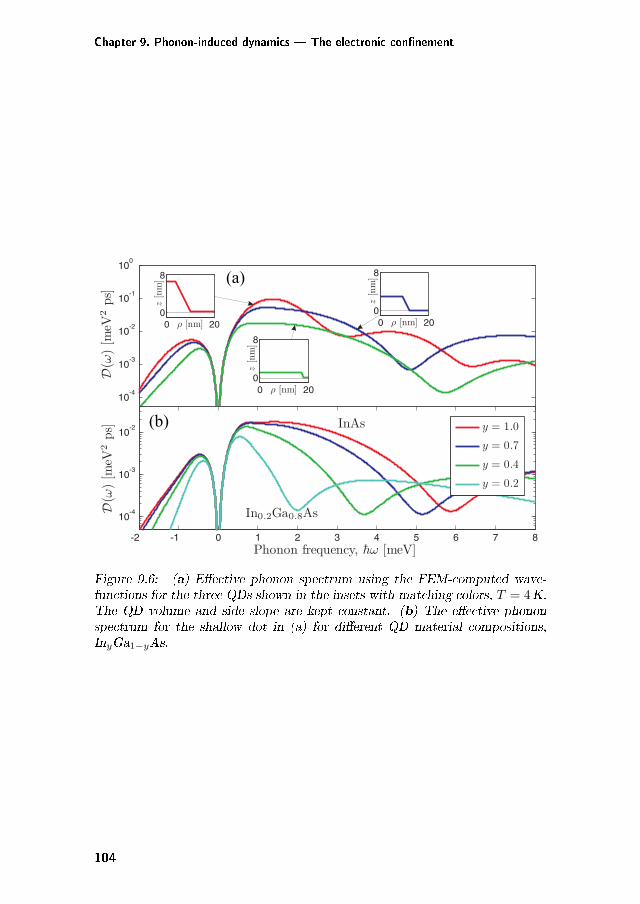
Chapter 9. Phonon-induced dynamics — The electronic confinement
(a)
(b)
Figure 9.6: (a) Effective phonon spectrum using the FEM-computed wave-functions for the three QDs shown in the insets with matching colors, 𝑇 = 4K.The QD volume and side slope are kept constant. (b) The effective phononspectrum for the shallow dot in (a) for different QD material compositions,In𝑦Ga1−𝑦As.
104
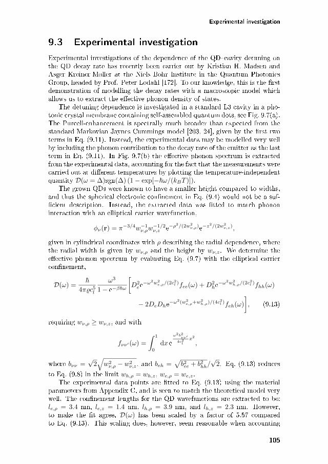
Experimental investigation
9.3 Experimental investigation
Experimental investigations of the dependence of the QD–cavity detuning onthe QD decay rate has recently been carrier out by Kristian H. Madsen andAsger Kreiner-Møller at the Niels Bohr Institute in the Quantum PhotonicsGroup, headed by Prof. Peter Lodahl [172]. To our knowledge, this is the firstdemonstration of modelling the decay rates with a macroscopic model whichallows us to extract the effective phonon density of states.
The detuning dependence is investigated in a standard L3 cavity in a pho-tonic crystal membrane containing self-assembled quantum dots, see Fig. 9.7(a).The Purcell-enhancement is spectrally much broader than expected from thestandard Markovian Jaynes Cummings model [203, 24], given by the first twoterms in Eq. (9.11). Instead, the experimental data may be modelled very wellby including the phonon contribution to the decay rate of the emitter as the lastterm in Eq. (9.11). In Fig. 9.7(b) the effective phonon spectrum is extractedfrom the experimental data, accounting for the fact that the measurements werecarried out at different temperatures by plotting the temperature-independentquantity 𝒟(𝜔 = ∆)sgn(∆) (1 − exp[−~𝜔/(𝑘𝐵𝑇 )]).
The grown QDs were known to have a smaller height compared to widths,and thus the spherical electronic confinement in Eq. (9.4) would not be a suf-ficient description. Instead, the extracted data was fitted to match phononinteraction with an elliptical carrier wavefunction,
𝜑𝜈(r) = 𝜋−3/4𝑤−1𝜈,𝜌𝑤
−1/2𝜈,𝑧 e−𝜌2/(2𝑤2
𝜈,𝜌)e−𝑧2/(2𝑤2𝜈,𝑧),
given in cylindrical coordinates with 𝜌 describing the radial dependence, wherethe radial width is given by 𝑤𝜈,𝜌 and the height by 𝑤𝜈,𝑧. We determine theeffective phonon spectrum by evaluating Eq. (9.7) with the elliptical carrierconfinement,
𝒟(𝜔) =~
4𝜋𝜚𝑐5𝑙
𝜔3
1 − e−𝛽~𝜔
[𝐷2
𝑒e−𝜔2𝑤2
𝑒,𝜌/(2𝑐2𝑙 )𝑓𝑒𝑒(𝜔) +𝐷2
ℎe−𝜔2𝑤2
ℎ,𝜌/(2𝑐2𝑙 )𝑓ℎℎ(𝜔)
− 2𝐷𝑒𝐷ℎe−𝜔2(𝑤2
𝑒,𝜌+𝑤2ℎ,𝜌)/(4𝑐
2𝑙 )𝑓𝑒ℎ(𝜔)
], (9.13)
requiring 𝑤𝜈,𝜌 ≥ 𝑤𝜈,𝑧, and with
𝑓𝜈𝜈′(𝜔) =
∫ 1
0
d𝑥 e𝜔2𝑏2
𝜈𝜈′4𝑐2
𝑙
𝑥2
,
where 𝑏𝜈𝜈 =√
2√𝑤2
𝜈,𝜌 − 𝑤2𝜈,𝑧, and 𝑏𝑒ℎ =
√𝑏2𝑒𝑒 + 𝑏2ℎℎ/
√2. Eq. (9.13) reduces
to Eq. (9.8) in the limit 𝑤ℎ,𝜌 = 𝑤ℎ,𝑧, 𝑤𝑒,𝜌 = 𝑤𝑒,𝑧.The experimental data points are fitted to Eq. (9.13) using the material
parameters from Appendix C, and is seen to match the theoretical model verywell. The confinement lengths for the QD wavefunctions are extracted to be:𝑙𝑒,𝜌 = 3.4 nm, 𝑙𝑒,𝑧 = 1.4 nm, 𝑙ℎ,𝜌 = 3.9 nm, and 𝑙ℎ,𝑧 = 2.3 nm. However,to make the fit agree, 𝒟(𝜔) has been scaled by a factor of 5.57 comparedto Eq. (9.13). This scaling does, however, seem reasonable when accounting
105
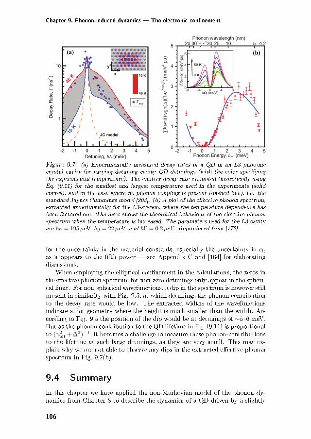
Chapter 9. Phonon-induced dynamics — The electronic confinement
(a) (b)
(ω=Δ)
ω
(ω=Δ)
Figure 9.7: (a) Experimentally measured decay rates of a QD in an L3 photoniccrystal cavity for varying detuning cavity–QD detunings (with the color specifyingthe experimental temperature). The emitter decay rate evaluated theoretically usingEq. (9.11) for the smallest and largest temperature used in the experiments (solidcurves), and in the case where no phonon coupling is present (dashed line), i.e. thestandard Jaynes Cummings model [203]. (b) A plot of the effective phonon spectrum,extracted experimentally for the L3-system, where the temperature dependence hasbeen factored out. The inset shows the theoretical behaviour of the effective phononspectrum when the temperature is increased. The parameters used for the L3 cavityare ~𝜅 = 195𝜇eV, ~𝑔 = 22𝜇eV, and ~Γ = 0.2𝜇eV. Reproduced from [172].
for the uncertainty in the material constants, especially the uncertainty in 𝑐𝑙,as it appears to the fifth power — see Appendix C and [164] for elaboratingdiscussions.
When employing the elliptical confinement in the calculations, the zeros inthe effective phonon spectrum for non-zero detunings only appear in the spheri-cal limit. For non-spherical wavefunctions, a dip in the spectrum is however stillpresent in similarity with Fig. 9.5, at which detunings the phonon-contributionto the decay rate would be low. The extracted widths of the wavefunctionsindicate a dot geometry where the height is much smaller than the width. Ac-cording to Fig. 9.5 the position of the dip would be at detunings of ∼5–6 meV.But as the phonon contribution to the QD lifetime in Eq. (9.11) is proportionalto (𝛾2tot+∆2)−1, it becomes a challenge to measure these phonon-contributionsto the lifetime at such large detunings, as they are very small. This may ex-plain why we are not able to observe any dips in the extracted effective phononspectrum in Fig. 9.7(b).
9.4 Summary
In this chapter we have applied the non-Markovian model of the phonon dy-namics from Chapter 8 to describe the dynamics of a QD driven by a slightly
106
Summary
detuned laser. We expanded this to consider the decay dynamics of a QD insidean optical cavity. In both cases we predict how that electron-phonon scatteringmay be suppressed due to differences in the spatial confinement of electrons andholes. Physically we explain this by a balancing between the electronic confine-ment and the effect on the deformation potential coupling on the energy bandsin the QD. We suggest that the effect may be measured by photoluminescenceexcitation spectroscopy, but also that it should strongly affect the decoherenceproperties of cavity QED systems.
We derived an expression for the phonon spectrum of ellipsoidal wavefunc-tions of the electrons and holes, and it is able to reproduce recent experimentalresults very well. In the experiment, we were however not able to observe anyof the dips in the effective phonon spectrum due to the electron-hole asym-metry. The wavefunction dimensions extracted from the experiment estimatesthat the dip in the phonon spectrum appear for QD–cavity detunings of ∼ 4-5meV. But at these detuning values, the phonon contribution to the measuredlifetime is also very low according to Eq. (9.11), making the dip very difficultto measure. In another recent experiment in Ref. [198], a dip is observed in theintensity spectrum of a QD pumped by a detuned laser at a detuning of ∼ 1meV, which could be due to these electron-hole asymmetries. It was, however,not possible to facilitate a collaboration for further investigations.
We demonstrated in Eq. (9.12) that the phonon-induced dephasing has twocontributions: In the long time limit depends on sampling the effective phononspectrum at two specific points, 𝒟(𝜔 = ±
√∆2 + 4𝑔2). In the short-time limit,
however, phonons may participate in non-energy-conserving virtual processes,which corresponds to sampling the effective phonon at all frequencies. Both ofthese contributions have to be minimized in order to reduce the phonon-induceddephasing the most.
In later works [73, 49], P. Kaer et al. have specifically investigated how thephonon-induced dephasing affects the indistingushability of photons emittedfrom a single-photon source created with a QD inside an optical cavity such asa micropillar. Here it is shown that the short-time non-Markovian interactionhas the largest significance on the indistinguishability of the emitted photons.These effects are minimized when the integral of the effective phonon spectrumis minimized, shown by the inset in Fig. 9.4, providing optical values of theelectronic and hole confinements. One must however keep in mind, that thesedepend on the material parameters of the quantum dot and the barrier.
We expect this new approach for suppressing phonon interactions to beimportant for the reduction of decoherence in devices for quantum informationtechnology, like single-photon sources and switches. This is combined with thepossibility of also engineering the phononic confinement, as will be discussedin the following chapter.
107

Chapter 10
Phonon-induced dynamics
— The phononic
confinement
In experimental setups which employ QDs, a bulk description of the phononsis usually employed, even though the sample with the QDs have a finite ex-tent. The question is, however, for which structures the bulk assumption isvalid, and whether the confinement of phonon may be exploited to improvethe performance of a quantum system, i.e. to improve the performance of asingle-photon source.
The simplest approach to consider phonon confinement is by confining themin a single spatial direction, i.e. in an infinite slab. It is well-known that thephonon reservoir changes properties when describing the coupling to a QD closeto a surface [204, 205]. These descriptions have been expanded to include theinfinite slab structure, where the calculations show that the emitted phononshave a possibility of being scattered at the surface and interact with the QDcarriers again, which will introduce modulations in the QD absorption spectrum[206, 207, 193].
A specific interest has been in predicting the dynamics in a double-quantumdot system placed in an infinite slab [208]. The double-dot systems are viablecandidates as solid-state qubits with the qubit states represented by an excita-tion in either of the dots, where the coefficients of the system may be controlledby electrically controlling the tunneling rate between the qubits. The perfor-mance of the qubits are, however, deteriorated by phonon-assisted couplingbetween the quantum dots. By placing the emitters at optimal positions in theslab, the phonon-induced effects may however be suppressed, due to changesin the phonon modes as compared to bulk phonons [208, 209, 210, 211].
In this chapter, we extend the approaches above to investigate how thesesuppressions apply to a cavity–QD-system suspended in an infinite slab. Usingthe theory from the previous chapters we have an approach to directly addressthe phonon reservoir. Physically such a system could correspond to the L3
109
Chapter 10. Phonon-induced dynamics — The phononic confinement
cavity in a photonic crystal slab as in Section 9.3. We show how the decay rateof the emitter may be either enhanced or suppressed (compared to bulk), de-pending on the detuning from the cavity modes. The enhancement/suppressiondepends on the energies of the vibrational modes in the slab, and we show howa slight change in the detuning can alter the phononic contribution to the decayrate significantly. The enhancement or reduction is most significant when theslab is thinnest, and we estimate that for a slab thickness of more than ∼ 70nm, a bulk description of the phonon modes is sufficient.
In Section 10.1 the vibrational modes of an infinite slab is described, andwe discuss the changes in the electron-phonon coupling mechanism as com-pared to bulk phonons. The resulting dynamics are calculated in Section 10.2,and the effective phonon spectrum is determined. The results are based onReducing dephasing in coupled quantum dot-cavity systems by engineering thecarrier wavefunctions. Proceedings of SPIE, the International Society for Op-tical Engineering 8271, 82710E (2012) by A. Nysteen, P. K. Nielsen, and J.Mørk.
10.1 Phonon modes in an infinite slab
For an isotropic elastic continuum the ion displacement at a position r obeysthe wave equation [206],
𝜕2𝑡 u = 𝑐2𝑡∇2u + (𝑐2𝑙 − 𝑐2𝑡 )∇(∇ ·u), (10.1)
where 𝑐𝑡 and 𝑐𝑙 are the velocity of the transverse and longitudinal sound wavesin bulk semiconductors, respectively, and obey 𝑐𝑙 > 𝑐𝑡. The boundary condi-tions to Eq. (10.1) stem from the assumption of a free-standing slab, requiringthat the normal components of the stress tensor vanish at the slab surface. Forthe vibrational modes in an infinite slab, the solution of Eq. (10.1) is on theform
u(r, 𝑡) =∑𝑛
∫u𝑛(k‖, 𝑧)e
ik‖ · r‖−i𝜔𝑛𝑡dk‖
(2𝜋)2, (10.2)
where the phonons are described by a continuum of plane waves in the in-plane directions and by a discrete set of eigenmodes u𝑛(k‖, 𝑧) in the 𝑧-directiondepending on the in-plane wavevector, k‖ [206].
Typically, vibrational modes of a slab are divided into shear, dilatationaland flexural waves [193]. According to Eq. (8.3), the deformation potential cou-pling allows coupling only between electrons and longitudinal acoustic phononswith the assumptions discussed in Section 8.1, and thus the shear waves willnot be considered. Examples of the grid displacements for dilatational andflexural modes are shown in Fig. 10.1.
Following [193, 212], the carrier–phonon interaction matrix element for thedeformation potential interaction for dilatational modes simplifies to
𝑀𝑛,𝜈𝜈 = 𝐷𝜈𝒢𝑛ℱ𝑛,𝜈 , (10.3)
where 𝐷𝜈 is the deformation potential of the electron/hole, and 𝒢𝑛 is a factorcontaining the dispersion relation of the phonon subband 𝑛, 𝜔𝑛. The spatial
110
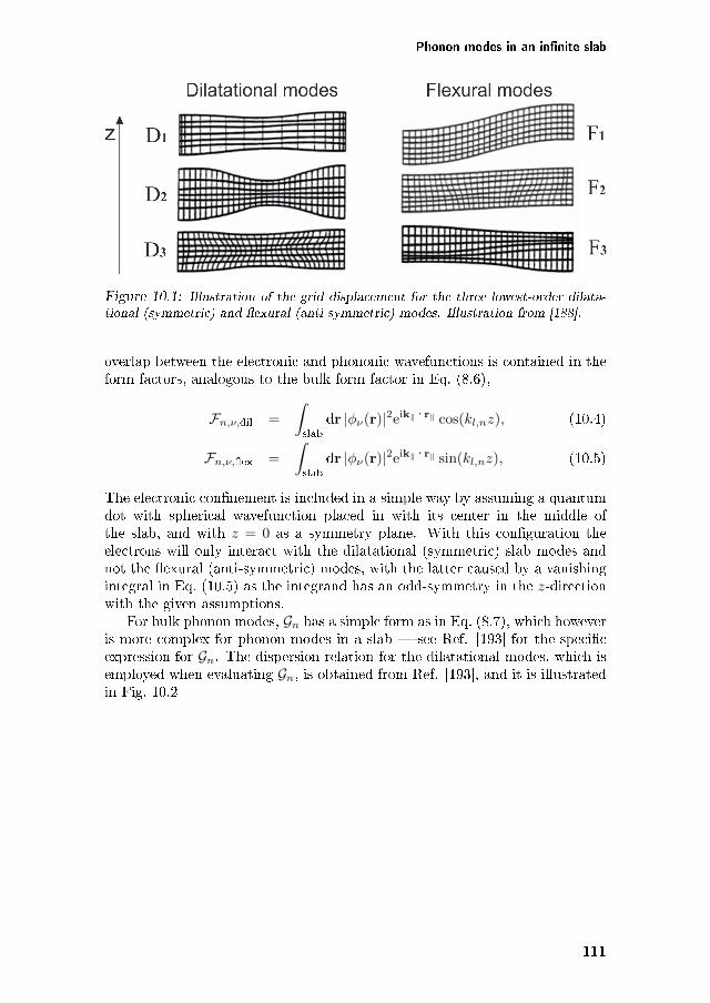
Phonon modes in an infinite slab
Figure 10.1: Illustration of the grid displacement for the three lowest-order dilata-tional (symmetric) and flexural (anti-symmetric) modes. Illustration from [188].
overlap between the electronic and phononic wavefunctions is contained in theform factors, analogous to the bulk form factor in Eq. (8.6),
ℱ𝑛,𝜈,dil =
∫slab
dr |𝜑𝜈(r)|2eik‖ · r‖ cos(𝑘𝑙,𝑛𝑧), (10.4)
ℱ𝑛,𝜈,flex =
∫slab
dr |𝜑𝜈(r)|2eik‖ · r‖ sin(𝑘𝑙,𝑛𝑧), (10.5)
The electronic confinement is included in a simple way by assuming a quantumdot with spherical wavefunction placed in with its center in the middle ofthe slab, and with 𝑧 = 0 as a symmetry plane. With this configuration theelectrons will only interact with the dilatational (symmetric) slab modes andnot the flexural (anti-symmetric) modes, with the latter caused by a vanishingintegral in Eq. (10.5) as the integrand has an odd-symmetry in the 𝑧-directionwith the given assumptions.
For bulk phonon modes, 𝒢𝑛 has a simple form as in Eq. (8.7), which howeveris more complex for phonon modes in a slab — see Ref. [193] for the specificexpression for 𝒢𝑛. The dispersion relation for the dilatational modes, which isemployed when evaluating 𝒢𝑛, is obtained from Ref. [193], and it is illustratedin Fig. 10.2
111
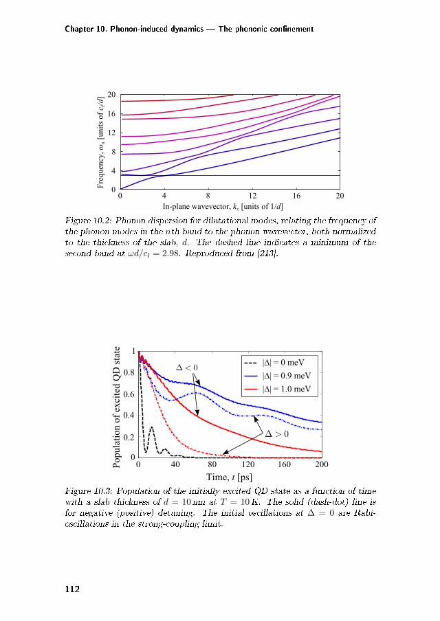
Chapter 10. Phonon-induced dynamics — The phononic confinement
0
20
0 20
4
12
8
16
4 8 12 16In-plane wavevector, kx [units of 1/d]
Fre
quen
cy, ω
n [
unit
s of
cl/d]
Figure 10.2: Phonon dispersion for dilatational modes, relating the frequency ofthe phonon modes in the 𝑛th band to the phonon wavevector, both normalizedto the thickness of the slab, 𝑑. The dashed line indicates a minimum of thesecond band at 𝜔𝑑/𝑐𝑙 = 2.98. Reproduced from [213].
Pop
ulat
ion,
of,e
xcit
ed,Q
D,s
tate 1
0.8
0.6
0.4
0.2
00 40 80 120 160 200
|∆|,=,1.0,meV
|∆|,=,0.9,meV
|∆|,=,0,meV
Time,,t,[ps]Figure 10.3: Population of the initially excited QD state as a function of timewith a slab thickness of 𝑑 = 10 nm at 𝑇 = 10K. The solid (dash-dot) line isfor negative (positive) detuning. The initial oscillations at ∆ = 0 are Rabi-oscillations in the strong-coupling limit.
112
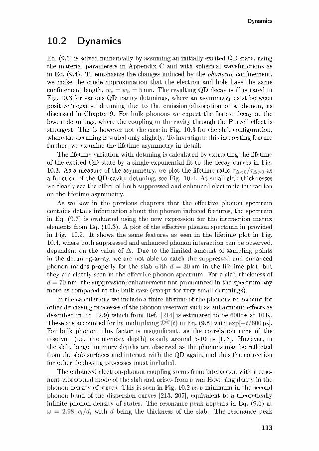
Dynamics
10.2 Dynamics
Eq. (9.5) is solved numerically by assuming an initially excited QD state, usingthe material parameters in Appendix C and with spherical wavefunctions asin Eq. (9.4). To emphasize the changes induced by the phononic confinement,we make the crude approximation that the electron and hole have the sameconfinement length, 𝑤𝑒 = 𝑤ℎ = 5nm. The resulting QD decay is illustrated inFig. 10.3 for various QD–cavity detunings, where an asymmetry exist betweenpositive/negative detuning due to the emission/absorption of a phonon, asdiscussed in Chapter 9. For bulk phonons we expect the fastest decay at thelowest detunings, where the coupling to the cavity through the Purcell effect isstrongest. This is however not the case in Fig. 10.3 for the slab configuration,where the detuning is varied only slightly. To investigate this interesting featurefurther, we examine the lifetime asymmetry in detail.
The lifetime variation with detuning is calculated by extracting the lifetimeof the excited QD state by a single-exponential fit to the decay curves in Fig.10.3. As a measure of the asymmetry, we plot the lifetime ratio 𝜏Δ<0/𝜏Δ>0 asa function of the QD-cavity detuning, see Fig. 10.4. At small slab thicknesseswe clearly see the effect of both suppressed and enhanced electronic interactionon the lifetime asymmetry.
As we saw in the previous chapters that the effective phonon spectrumcontains details information about the phonon-induced features, the spectrumin Eq. (9.7) is evaluated using the new expression for the interaction matrixelements from Eq. (10.3). A plot of the effective phonon spectrum in providedin Fig. 10.5. It shows the same features as seen in the lifetime plot in Fig.10.4, where both suppressed and enhanced phonon interaction can be observed,dependent on the value of ∆. Due to the limited amount of sampling pointsin the detuning-array, we are not able to catch the suppressed and enhancedphonon modes properly for the slab with 𝑑 = 30nm in the lifetime plot, butthey are clearly seen in the effective phonon spectrum. For a slab thickness of𝑑 = 70 nm, the suppression/enhancement not pronounced in the spectrum anymore as compared to the bulk case (except for very small detunings).
In the calculations we include a finite lifetime of the phonons to account forother dephasing processes of the phonon reservoir such as anharmonic effects asdescribed in Eq. (2.9) which from Ref. [214] is estimated to be 600 ps at 10K.These are accounted for by multiplying 𝒟≷(𝑡) in Eq. (9.6) with exp[−𝑡/600 ps].For bulk phonon, this factor is insignificant, as the correlation time of thereservoir (i.e. the memory depth) is only around 5-10 ps [173]. However, inthe slab, longer memory depths are observed as the phonons may be reflectedfrom the slab surfaces and interact with the QD again, and thus the correctionfor other dephasing processes must included.
The enhanced electron-phonon coupling stems from interaction with a reso-nant vibrational mode of the slab and arises from a van-Hove singularity in thephonon density of states. This is seen in Fig. 10.2 as a minimum in the secondphonon band of the dispersion curves [213, 207], equivalent to a theoreticallyinfinite phonon density of states. The resonance peak appears in Eq. (9.6) at𝜔 = 2.98 · 𝑐𝑙/𝑑, with 𝑑 being the thickness of the slab. The resonance peak
113
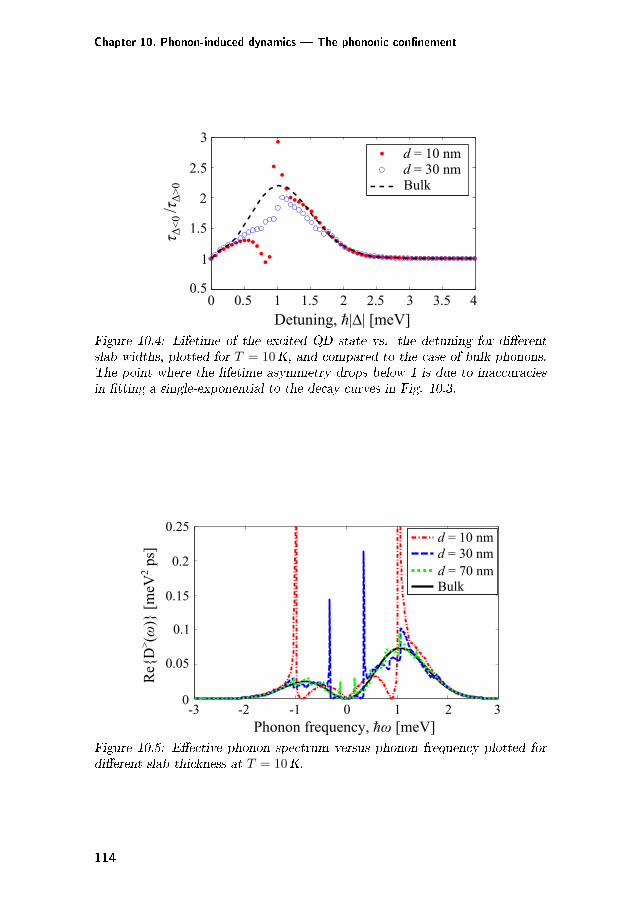
Chapter 10. Phonon-induced dynamics — The phononic confinement
Detuning, h|∆| [meV]
τΔ
<0 /τΔ
>0
0 0.5 1 1.5 2 2.5 3 3.5 40.5
1
1.5
2
2.5
3d = 10 nmd = 30 nmBulk
Figure 10.4: Lifetime of the excited QD state vs. the detuning for differentslab widths, plotted for 𝑇 = 10K, and compared to the case of bulk phonons.The point where the lifetime asymmetry drops below 1 is due to inaccuraciesin fitting a single-exponential to the decay curves in Fig. 10.3.
dr=r10rnmdr=r30rnm
Bulk
Re
D>(ω
)r[
meV
2 rps]
0.25
0.2
0.15
0.1
0.05
0
Phononrfrequency,rhωr[meV]-3 -2 -1 0 1 2 3
dr=r70rnm
Figure 10.5: Effective phonon spectrum versus phonon frequency plotted fordifferent slab thickness at 𝑇 = 10K.
114
Summary
moves closer to 𝜔 = 0 as the thickness of the slab increases. However, the am-plitude of the resonance peak will decrease with increasing 𝑑, since a phononemitted from the QD has a smaller probability of interacting with the surfacerather than disappearing into the infinite extend of the slab. At 𝑑 = 10nm thetravel time for a photon from the QD to the surface and back is ∼ 4 ps, whichexactly corresponds to the fast oscillations in Fig. 10.3 for non-zero detuning.
Surprisingly, at slightly lower detunings than for the enhanced phononmodes, the interaction with the phonon modes is suppressed, which accord-ing to Eq. (9.11) gives the zeros in the lifetime asymmetry plot in Fig. 10.4.This system thus shows features of a coupled QD-cavity system where the sys-tem at a specific detuning does not experience any phonon-induced lifetimeasymmetry, even when assuming identical widths of the wavefunction for theelectron and the hole.
We should emphasize the assumptions and approximations made for thecalculations. The large spikes in the effective phonon spectrum correspond to astrong electron-phonon interaction, which in the theory is assumed only to be aweak perturbation in Eq. (8.22). In a system where these phonon resonances isto be exploited, the assumption of small interaction strength should be tested.Furthermore, if very narrow slabs are used, the contrast between the GaAsmaterial and the surrounding air introduces a quantum well for the electronsas well, which has to be taken into account. A full description where theflexural slab modes have to be taken into account, if we want to consider thepossibility of placing the QD away from the center plane of the slab, or if wetreat non-symmetric electronic wavefunction.
10.3 Summary
In conclusion we have demonstrated how the presence of an infinite slab arounda coupled cavity-quantum dot system alters the dynamics significantly dueto enhanced/suppressed electron-phonon interaction depending on the cavity-quantum dot detuning. The enhancement/suppression depends on how theQD–cavity detuning matches the vibrational modes of the slab, and by changingthe detuning only slightly ∼ 0.3 meV, the phonon contribution to the decayrate of the emitter may go from 0 to a large enhancement compared to the bulkcase. We estimate that for a slab thickness of ∼ 70 nm, the bulk descriptionof the phonon modes is sufficient. In the experiment in Section 9.3, a slabthickness of ∼ 150 nm was used, and the considerations in this chapter justifythe bulk treatment of the phonons.
We believe that these effects of confining the phonons may have interestingapplications in the creation of a coupled QD-cavity system with low dephasing,showing promising features e.g. for obtaining high indistinguishability in single-photon sources. An interesting perspective of the calculations would be toconsider micropillar single-photon sources [32, 215]. Here the phonons areconfined effectively in two dimensions, where one thus would expect a highersensitivity of the phonon modes to confinement dimensions than compared tothe slab. The electron-phonon interaction matrix elements will, however, alsobecomes more complex.
115

Chapter 11
Highlights and outlook
The work carried out in this thesis provides a fundamental description ofphoton–photon interaction in the presence of non-linearities such as a two-levelsystem, and we discuss implementations, possibilities, and limitations whenexploiting the non-linearities in conditional gates for quantum computation.When utilising solid-state implementations of the few-photon non-linearitiessuch as semiconductor quantum dots, coupling to phonons may deterioratethe efficiency, and we discuss possibilities for suppressing the phonon-inducedeffects by manipulating the electronic and phononic confinement.
Highlights
We focus on a simple system in which propagating photons interact via a mate-rial non-linearity, namely in an infinite waveguide containing a two-level emit-ter. Single-photon scattering is well-understood, but the dynamics becomesmuch more complex for two-photon scattering due to saturation of the emitter.We consider two approaches for examining non-trivial two-photon interactions;a numerical wavefunction approach and the scattering matrix formalism. Thewavefunction approach excels in determining the total system wavefunction atall times and makes it possible to relate the emitter excitation to the scattering-induced correlations. It may easily be expanded to consider more complicatedscatterers, e.g. multiple quantum dots in a cavity or spatially separated scat-teres. On the other hand, the scattering matrix formalism allows calculation ofthe scattered state faster than the full numerical approach. However, it relieson the calculation of a scatterer-specific two-photon scattering matrix whichattains a simple expression for the simple two-level scatterer, but quickly be-comes much more complex to evaluate if the scatterer is more complex.
With the two approaches we demonstrate that the largest non-linearity-induced correlations between two photons scattering on an emitter occurs whenthe emitter is excited the most. This happens when the bandwidth of theincoming photon pulses is similar to the linewidth of the emitter. For scatteringof two initially counter-propagating photons we show how the emitter worksas a non-linear beam splitter in this regime of input pulse bandwidths. We
117
Chapter 11. Highlights and outlook
demonstrate how the non-linearity may help preserving the spectral shapesof the photons. Even when accounting for all the scattering-induced changesphase and spectrum of the photons, the photon properties are preserved withalmost 80 % in the non-linear beam splitter.
By employing the gained knowledge, we propose an experimental setupfor a controlled-phase gate consisting of passive optical components and twoemitters. We estimate a gate fidelity close to 80 %, limited by phase mod-ulations upon scattering and inherent errors from four-wave-mixing processescaused by the non-linearity. We discuss another proposal for a controlled-phasegate consisting of a waveguide coupling to two ring resonators with a strongsecond-order non-linearity. The scheme suppresses the four-wave-mixing pro-cesses by dynamically capturing the first of two temporally separated photons.Theoretically the scheme promises higher fidelities than the other gate pro-posal, although the dynamical capturing relies on precise timing and controlover cavity detunings, which in reality may be very difficult with the currenttechnology.
When the non-linearities are implemented in solid-state environments, cou-pling to phonons may induce dephasing, limiting the coherent interactions. Tounderstand how to minimize the phonon-induced effects, we apply a modelby P. Kaer [173] which considers a non-Markovian coupling to a large phononreservoir through the deformation potential coupling. We specifically inves-tigate how the electronic and phononic confinement affect the dynamics of aquantum dot decay through coupling to an optical cavity. The theory is ap-plied to an experimental measurement of the decay rate of a quantum dotinside an photonic crystal cavity, from which we are able to extract an effectivephonon spectrum. When examining the electronic confinement, we find thatthe asymmetry between the electron and hole wavefunction in a quantum dotin a GaAs platform may be exploited to suppress the phonon-induced effects.We explain this suppression by a balancing of the electron-hole wavefuntionand the deformation potential coupling, occuring only in materials where thedeformation interaction shifts the electron and hole energy bands in the samedirection. Regarding the confinement of the phonons, we consider a quantumdot–cavity system with the dot placed in the center of an infinite slab. Wedemonstrate how the phonon-assisted coupling of the dot through the cav-ity may be either significantly suppressed or enhanced, depending on how thequantum dot–cavity detuning matches the energies of the vibrational modesin the slab. Furthermore we estimate that a bulk description of the phononmodes is sufficient for a slab thickness larger than ∼ 70 nm, at least when de-scribing the phonon-contribution the emitter decay rate. We believe that a fullunderstanding of the possibilities of manipulating the electronic and phononicconfinements will be important for reducing dephasing in quantum devices suchas single-photon sources and non-linear gates.
Outlook and future directions
It is obvious that a large amount of work still has to be carried out in orderto achieve an efficient, scalable platform for performing quantum computation
118
utilising few-photon non-linearities. This is both in the field of creating efficientsingle-photon sources, gates, and detectors in a scalable scheme — and also incombining them together in integrated circuits without large coupling lossesbetween the different devices. In wake of recent breakthroughs, the followingyears will most likely bring many new achievements in the fundamental studyof strongly interacting photons. As an example of the recent breakthroughs, achiral spin-photon interface in a photonic crystal waveguide allows direction-specific emission to emitter depending on the spin state of a quantum dot[138]. New structures with non-linearities in the single-photon regime have alsoappeared, such as a graphene plasmon cavity coupling to a dielectric waveguide[216], which extends the perspectives of the possibilities with the few-photonnon-linearities.
It would indeed be interesting to expand the numerical code to considerseveral spatially separated emitters and/or cavities in the waveguide, especiallyregarding investigation of sharp Fano resonances [217]. These structures requirea significantly smaller energy detuning to change from being fully transmissiveto fully reflective, as compared to a system with only a single emitter. TheseFano-structures could high relevance when designing few-photon conditionalgates.
Regarding the phonon-induced effects it would be worth making a morethorough investigation of varying the material compositions in order to changethe electronic confinement and deformation potential constants such that thephonon-induced dephasing is suppressed the most in quantum devices. Wealso see promising perspectives in suppressing the dephasing by altering thephononic confinement, which may be done by an expansion of the presentedmodel to more complicated phonon confinements such as in micropillars. Thepossibility of creating structures with simultaneous photonic and phononicbandgap has already been proposed, although with the purpose of enhancingthe optomechanical coupling strength [218, 195]. The bandgap in the presentedstructures is, however, for vibrational modes with energies in the GHz regime,which are several magnitudes below the energies of the acoustic phonons. Itwould be interesting to examine if these structures could be exploited to sup-press dephasing from acoustical phonons in the quantum dot systems.
119

Appendix
121

Appendix A
Analytical derivation of
two-photon emitter
excitation
In this appendix we demonstrate how to find an analytical expression for theemitter excitation probability, when a two-photon pulse consisting of two co-phopagating, uncorrelated single-photon pulses scatters on an emitter, whichinitially is in its ground state. We specifically determine the excitation prob-ability for an input pulse consisting of two identical pulses with a Gaussianwavepacket, and we use this to verify the numerical implementation demon-strated in Chapter 4.
The procedure of the derivation follows Kojima et al. [91] and Valente etal. [92], starting from the Hamiltonian in Eq. (3.1), with the waveguide modesgiven as plane wave modes with a frequency 𝜈. The waveguide modes are splitinto two subgroups, 𝑎 and 𝑏, distinguished by the direction of propagating, andwith different orientations of the spatial axis of the two modes, by which wemay assume a positive value of the wavevector for all modes (removing theabsolute value in the dispersion relation, Eq. (3.4)). With these notations, theHamiltonian is
𝐻 = 𝐻1D +𝐻atom +𝐻int, (A.1)
𝐻1D =
∞∑𝜈=0
~𝜈(𝑎†𝜈𝑎𝜈 + 𝑏†𝜈𝑏𝜈), (A.2)
𝐻atom = ~𝜈𝐴𝑐†𝑐, (A.3)
𝐻int = −i
∞∑𝜈=0
~𝑔𝑎𝜈 [𝑎𝜈𝑐† − 𝑐𝑎†𝜈 ] − i
∞∑𝜈=0
~𝑔𝑏𝜈 [𝑏𝜈𝑐† − 𝑐𝑏†𝜈 ], (A.4)
where 𝑎†𝜈 and 𝑏†𝜈 creates an excitation of frequency 𝜈 in the respective subgroupof waveguide modes, and 𝑐† creates an excitation in the emitter. Here 𝜈𝐴 is thetransmission frequency of the emitter, and 𝑔𝑎𝜈 and 𝑔𝑏𝜈 describing the coupling
123
Appendix A. Analytical derivation of two-photon emitter excitation
strength of the emitter into the different directions of the waveguide. In thisderivation we use slightly different definitions of rotating frames etc. comparedto the remaining thesis, which however does not influence the results
We define the two-excitation state as,
|𝜓(𝑡)⟩ =
∞∑𝜈=0
𝜓𝑎𝜈 (𝑡)𝑎†𝜈𝑐
†|𝜑⟩ +
∞∑𝜈=0
𝜓𝑏𝜈(𝑡)𝑏†𝜈𝑐
†|𝜑⟩ +
∞∑𝜈1,𝜈2=0
[𝜑𝑎𝑎𝜈1𝜈2
(𝑡)𝑎†𝜈1𝑎†𝜈2
+ 𝜑𝑎𝑏𝜈1𝜈2(𝑡)𝑎†𝜈1
𝑏†𝜈2+ 𝜑𝑏𝑎𝜈1𝜈2
(𝑡)𝑏†𝜈1𝑎†𝜈2
+ 𝜑𝑏𝑏𝜈1𝜈2(𝑡)𝑏†𝜈1
𝑏†𝜈2
]|𝜑⟩. (A.5)
The factor of 1/√
2 used in Eq. (4.5) is absorbed into the expansion coefficientsof the state to ease the notation in the following for 𝜑𝑎𝑎 and 𝜑𝑏𝑏 (changing thenormalization condition of the state). Furthermore we define the symmetricversion of 𝜑,
Φ𝜎1𝜎2𝜈1𝜈2
=𝜑𝜎1𝜎2𝜈1𝜈2
+ 𝜑𝜎2𝜎1𝜈2𝜈1
2. (A.6)
The expressions above are inserted in the time-dependent Schrödinger equa-tion i~𝜕𝑡|𝜓(𝑡)⟩ = 𝐻|𝜓(𝑡)⟩. By projecting onto the different system states givenin Eq. (A.5), a system of coupled differential equations is achieved,
𝜕𝑡𝜓𝜎𝑤 = −i(𝜈𝐴 + 𝑤)𝜓𝜎
𝑤 − 2∑𝜈2
(𝑔𝜎𝜈2
Φ𝜎𝜎𝑤𝜈2
+ 𝑔𝜈2Φ𝜎
𝑤𝜈2
), (A.7a)
𝜕𝑡Φ𝜎1𝜎2𝑤1𝑤2
= −i(𝑤1 + 𝑤2)Φ𝜎1𝜎2𝑤1𝑤2
+1
2
(𝑔𝜎2𝑤2𝜓𝜎1𝑤1
+ 𝑔𝜎1𝑤1𝜓𝜎2𝑤2
), (A.7b)
where 𝜎 ∈ 𝑎, 𝑏, and is the opposite of 𝜎, i.e. = 𝑏. Defining the Fouriertransform
𝜓𝜎(𝑟, 𝑡) =
∞∑𝜈=0
𝜓𝜎𝜈 (𝑡)ei𝑘𝜈𝑟, (A.8)
and using the relation∑𝜈
𝜈𝜓𝜎𝜈 ei𝑘𝜈𝑟 = −i𝑐𝜕𝑟
∑𝜈
𝜓𝜎𝜈 ei𝑘𝜈𝑟, (A.9)
Eq. (A.7a) becomes
[𝜕𝑡 + 𝑐𝜕𝑟]𝜓𝜎(𝑟, 𝑡) = −i𝜈𝐴𝜓𝜎(𝑟, 𝑡) − 2
∑𝜈𝑤
(𝑔𝜎𝜈 Φ𝜎𝜎
𝑤𝜈(𝑡) + 𝑔𝜈 Φ𝜎𝑤𝜈(𝑡)
)ei𝑘𝑤𝑟.(A.10)
The term −i𝜈𝐴𝜓𝜎(𝑟, 𝑡) is removed by introducing a rotating frame [92],
𝜓𝜎(𝑡) = 𝜓𝜎(𝑡)ei𝜈𝐴𝑡ei𝜔𝜎𝐿(𝑡−𝑟/𝑐). (A.11)
With this, Eq. (A.10) becomes
[𝜕𝑡 + 𝑐𝜕𝑟]𝜓𝜎(𝑟, 𝑡) = −ei𝜈𝐴𝑡+i𝜈𝜎𝐿(𝑡−𝑟/𝑐)2
∑𝜈𝑤
(𝑔𝜎𝜈 Φ𝜎𝜎
𝑤𝜈 + 𝑔𝜈 Φ𝜎𝑤𝜈
)ei𝑘𝑤𝑟. (A.12)
124
To determine expressions for the Φ’s, we formally integrate Eq. (A.7b), assum-ing that the initial time is 𝑡 = 0,
Φ𝜎1𝜎2𝑤1𝑤2
(𝑡) = Φ𝜎1𝜎2𝑤1𝑤2
(0)e−i(𝑤1+𝑤2)𝑡
+1
2
∫ 𝑡
0
d𝑡′[𝑔𝜎2𝑤2𝜓𝜎1𝑤1
(𝑡′) + 𝑔𝜎1𝑤1𝜓𝜎2𝑤2
(𝑡′)]
e−i(𝑤1+𝑤2)(𝑡−𝑡′). (A.13)
Inserting this into Eq. (A.12), we arrive at
[𝜕𝑡 + 𝑐𝜕𝑟]𝜓𝜎(𝑟, 𝑡) = −𝐴𝜎1 (𝑟, 𝑡) −𝐴𝜎
2 (𝑟, 𝑡), (A.14)
where
𝐴𝜎1 (𝑟, 𝑡) = 2
∑𝑤𝑣
[𝑔𝜎𝑣 Φ𝜎𝜎
𝑤𝑣(0) + 𝑔𝜎𝑣 Φ𝜎𝜎𝑤𝑣(0)
]ei𝜈𝐴𝑡+i𝜈𝜎
𝐿(𝑡−𝑟/𝑐)−i(𝑤+𝑣)𝑡+i𝑘𝑤𝑟, (A.15)
and
𝐴𝜎2 (𝑟, 𝑡) = ei𝜈𝐴𝑡+i𝜈𝜎
𝐿(𝑡−𝑟/𝑐)∑𝑤𝑣2
[𝑔𝜎𝑣
∫ 𝑡
0
d𝑡′ [𝑔𝜎𝑣𝜓𝜎𝑤(𝑡′) + 𝑔𝜎𝑤𝜓
𝜎𝑣 (𝑡′)] e−i(𝑤+𝑣)(𝑡−𝑡′)
+𝑔𝜎𝑣
∫ 𝑡
0
d𝑡′[𝑔𝜎𝑣𝜓
𝜎𝑤(𝑡′) + 𝑔𝜎𝑤𝜓
𝜎𝑣 (𝑡′)
]e−i(𝑤+𝑣)(𝑡−𝑡′)
]ei𝑘𝑤𝑟. (A.16)
From here we make the Markov-approximation and thus assume that the cou-pling constants are independent of frequency, according to the discussion inSection 3.2.
Simplifying 𝐴𝜎2 (𝑟, 𝑡)
With Eq. (A.8), we may further divide 𝐴𝜎2 (𝑟, 𝑡) into four terms,
𝐴𝜎2,1(𝑟, 𝑡) = 𝑔𝜎𝑔𝜎
∫ 𝑡
0
d𝑡′ 𝜓𝜎(𝑟 − 𝑐(𝑡− 𝑡′), 𝑡′)∑𝜈
e−i𝜈(𝑡−𝑡′)+i𝜈𝐴𝑡+i𝜈𝜎𝐿(𝑡−𝑟/𝑐),
(A.17a)
𝐴𝜎2,2(𝑟, 𝑡) = 𝑔𝜎𝑔𝜎
∫ 𝑡
0
d𝑡′ 𝜓𝜎(−𝑐(𝑡− 𝑡′), 𝑡′)∑𝑤
e−i𝑤(𝑡−𝑡′)+i𝑘𝑤𝑟+i𝜈𝐴𝑡+i𝜈𝜎𝐿(𝑡−𝑟/𝑐),
(A.17b)
𝐴𝜎2,3(𝑟, 𝑡) = 𝑔𝜎𝑔𝜎
∫ 𝑡
0
d𝑡′ 𝜓𝜎(𝑟 − 𝑐(𝑡− 𝑡′), 𝑡′)∑𝜈
e−i𝜈(𝑡−𝑡′)+i𝜈𝐴𝑡+i𝜈𝜎𝐿(𝑡−𝑟/𝑐),
(A.17c)
𝐴𝜎2,4(𝑟, 𝑡) = 𝑔𝜎𝑔𝜎
∫ 𝑡
0
d𝑡′ 𝜓𝜎(−𝑐(𝑡− 𝑡′), 𝑡′)∑𝑤
e−i𝑤(𝑡−𝑡′)+i𝑘𝑤𝑟+i𝜈𝐴𝑡+i𝜈𝜎𝐿(𝑡−𝑟/𝑐),
(A.17d)
We consider each term separately. For the first term, Eq. (A.17a), we transform𝜓𝜎 to 𝜓𝜎 using Eq. (A.11),
𝐴𝜎2,1(𝑟, 𝑡) = 𝑔𝜎𝑔𝜎
∫ 𝑡
0
d𝑡′ 𝜓𝜎(𝑟 − 𝑐(𝑡− 𝑡′), 𝑡′)∑𝜈
e−i(𝜈−𝜈𝐴)(𝑡−𝑡′). (A.18)
125
Appendix A. Analytical derivation of two-photon emitter excitation
Using the Wigner–Weisskopf approximation as in Section 3.2, 𝜓 may be movedoutside the integral by assuming that it varies slowly compared to the temporalevolution in the exponential. The remaining part in the integral over timecorresponds to half a delta-function (plus a Lamb shift), leading to a definitionof the decay rate
Γ𝜎1𝜎2 = 2𝜋𝑔𝜎1𝑔𝜎2
∑𝜈
𝛿(𝜈 − 𝜈𝐴), (A.19)
leading to
𝐴𝜎2,1(𝑟, 𝑡) =
Γ𝜎𝜎
2𝜓(𝑟, 𝑡). (A.20)
A similar statement applies to 𝐴𝜎2,3(𝑟, 𝑡) in Eq. (A.17c), which becomes
𝐴𝜎2,3(𝑟, 𝑡) =
Γ𝜎𝜎
2𝜓(𝑟, 𝑡). (A.21)
For Eq. (A.17b), we get
𝐴𝜎2,2(𝑟, 𝑡) = 𝑔𝜎𝑔𝜎e−i𝛿𝜎𝐿𝑟/𝑐
∫ 𝑡
0
d𝑡′ 𝜓𝜎(−𝑐(𝑡− 𝑡′), 𝑡′)∑𝑤
e−i(𝑤−𝜈𝐴)(𝑡−𝑡′−𝑟/𝑐),
(A.22)
where 𝛿𝜎𝐿 = 𝜈𝜎𝐿−𝜈𝐴 and 𝑘𝑤 = 𝑤/𝑐. Making that same assumption about a fastvarying exponential, the only contribution to the 𝑤-sum is when 𝑡−𝑡′−𝑟/𝑐 = 0.As the integration only goes from 0 < 𝑡′ < 𝑡, this introduces two Heaviside stepfunction,
𝐴𝜎2,2(𝑟, 𝑡) = e−i𝛿𝜎𝐿𝑟/𝑐Γ𝜎𝜎𝜃(𝑟)𝜃(𝑡− 𝑟/𝑐)𝜓𝜎(−𝑟, 𝑡− 𝑟/𝑐), (A.23)
with the propertiy that 𝜃(0) ≡ 1/2.The last contribution in Eq. (A.17d) becomes
𝐴𝜎2,4(𝑟, 𝑡) = 𝑔𝜎𝑔𝜎e−i𝛿𝜎𝐿𝑟/𝑐+i(𝜈𝜎
𝐿−𝜈𝜎𝐿)𝑡
∫ 𝑡
0
d𝑡′ 𝜓𝜎(−𝑐(𝑡− 𝑡′), 𝑡′)
×∑𝑤
e−i(𝑤−𝜈𝐴)(𝑡−𝑡′−𝑟/𝑐). (A.24)
With similar arguments as for 𝐴𝜎2,2(𝑟, 𝑡), we arrive at
𝐴𝜎2,4(𝑟, 𝑡) = e−i𝛿𝜎𝐿𝑟/𝑐+i(𝜈𝜎
𝐿−𝜈𝜎𝐿)𝑡Γ𝜎𝜎𝜃(𝑟)𝜃(𝑡− 𝑟/𝑐)𝜓𝜎(−𝑟, 𝑡− 𝑟/𝑐). (A.25)
Thus Eq. (A.14) simplifies to
[𝜕𝑡 + 𝑐𝜕𝑟]𝜓𝜎(𝑟, 𝑡) = 𝐴𝜎1 (𝑟, 𝑡) − Γ𝜎𝜎 + Γ𝜎𝜎
2𝜓𝜎(𝑟, 𝑡)
− 𝜃(𝑟)𝜃(𝑡− 𝑟/𝑐)e−i𝛿𝜎𝐿𝑟/𝑐
[Γ𝜎𝜎𝜓𝜎(−𝑟, 𝑡− 𝑟/𝑐) + Γ𝜎𝜎ei(𝜈
𝜎𝐿−𝜈𝜎
𝐿)𝑡𝜓𝜎(−𝑟, 𝑡− 𝑟/𝑐)
],
(A.26)
where 𝐴𝜎1 (𝑟, 𝑡) only depends on the initial conditions of the 𝜑s. We define the
total rate Γ = Γ𝜎𝜎 + Γ𝜎𝜎 = Γ𝑎𝑎 + Γ𝑏𝑏, which according to Eq. (A.26) describesthe rate of spontaneous emission of the emitter into both directions.
126
Solving Eq. (A.26)
To determine a solution to Eq. (A.26), we first consider a general differentialequation on the form
[𝜕𝑡 + 𝑐𝜕𝑟]𝑓(𝑟, 𝑡) = −Γ𝑓(𝑟, 𝑡) −𝐴(𝑟, 𝑡). (A.27)
Applying a symmetric Fourier transform,
𝑓(𝑘, 𝑡) =1√2𝜋
∫d𝑟 𝑓(𝑟, 𝑡)e−i𝑘𝑟, 𝑓(𝑟, 𝑡) =
1√2𝜋
∫d𝑘 𝑓(𝑘, 𝑡)ei𝑘𝑟, (A.28)
Eq. (A.27) becomes
[𝜕𝑡 + i𝑘𝑐+ Γ]𝑓(𝑘, 𝑡) = − 1√2𝜋
∫d𝑟 𝐴(𝑟, 𝑡)e−i𝑘𝑟. (A.29)
By multiplying each side with exp[(Γ + i𝑘𝑐)𝑡] and integrating over time, wearrive at
𝑓(𝑘, 𝑡) = 𝑓(𝑘, 0)e−(Γ+i𝑘𝑐)𝑡 − 1√2𝜋
∫ 𝑡
0
d𝑡′∫
d𝑟 𝐴(𝑟, 𝑡′)e−i𝑘𝑟−(Γ+i𝑘𝑐)(𝑡−𝑡′).
(A.30)
Transforming back, we get
𝑓(𝑟, 𝑡) =1√2𝜋
∫d𝑘 𝑓(𝑘, 0)e−(Γ+i𝑘𝑐)𝑡+i𝑘𝑟
− 1
2𝜋
∫d𝑘∫ 𝑡
0
d𝑡′∫
d𝑟′𝐴(𝑟′, 𝑡′)e−i𝑘𝑟′−(Γ+i𝑘𝑐)(𝑡−𝑡′)+i𝑘𝑟
= 𝑓(𝑟 − 𝑐𝑡, 0)e−Γ𝑡 −∫ 𝑡
0
d𝑡′∫
d𝑟 𝐴(𝑟′, 𝑡′)𝛿(𝑟 − 𝑟′ − 𝑐(𝑡− 𝑡′))e−Γ(𝑡−𝑡′)
= 𝑓(𝑟 − 𝑐𝑡, 0)e−Γ𝑡 −∫ 𝑡
0
d𝑡′𝐴 (𝑟 − 𝑐(𝑡− 𝑡′), 𝑡′) e−Γ(𝑡−𝑡′). (A.31)
This derived expression may be used to solve Eq. (A.26). By defining
𝐵𝜎(𝑟, 𝑡) =
∫ 𝑡
0
d𝑡′𝐴𝜎1 (𝑟 − 𝑐(𝑡− 𝑡′), 𝑡′) e−Γ(𝑡−𝑡′)/2, (A.32)
we may use Eq. (A.31) to write the solution for Eq. (A.26),
𝜓𝜎(𝑟, 𝑡) = 𝜓(𝑟 − 𝑐𝑡, 0)e−Γ𝑡/2 −𝐵𝜎(𝑟, 𝑡)
−∫ 𝑡
0
d𝑡′ 𝜃(𝑟 − 𝑐(𝑡− 𝑡′))𝜃(𝑡− 𝑟/𝑐)e−i𝛿𝜎𝐿(𝑟−𝑐(𝑡−𝑡′))/𝑐
×[Γ𝜎𝜎𝜓𝜎(−(𝑟 − 𝑐(𝑡− 𝑡′)), 𝑡− 𝑟/𝑐)
+ Γ𝜎𝜎ei(𝜈𝜎𝐿−𝜈𝜎
𝐿)𝑡𝜓𝜎(−(𝑟 − 𝑐(𝑡− 𝑡′)), 𝑡− 𝑟/𝑐)
]e−Γ(𝑡−𝑡′)/2. (A.33)
127
Appendix A. Analytical derivation of two-photon emitter excitation
For simplicity, we assume from here that 𝜈𝜎𝐿 = 𝜈𝜎𝐿 ≡ 𝜈𝐿, i.e. that the carrierfrequency of the incoming pulses is identical in both arms. We write Eq. (A.33)in a simple-looking form,
𝜓𝜎(𝑟, 𝑡) = 𝜓(𝑟 − 𝑐𝑡, 0)e−Γ𝑡/2 −𝐵𝜎(𝑟, 𝑡) − Γ𝜎𝜎𝐷𝜎(𝑟, 𝑡) − Γ𝜎𝜎𝐷𝜎(𝑟, 𝑡), (A.34)
with
𝐷𝜎1(𝑟, 𝑡) = 𝜃(𝑡− 𝑟/𝑐)
∫ 𝑡
0
d𝑡′ 𝜃(𝑟 − 𝑐(𝑡− 𝑡′))e−i𝛿𝐿(𝑟−𝑐(𝑡−𝑡′))/𝑐
× 𝜓𝜎1(−(𝑟 − 𝑐(𝑡− 𝑡′)), 𝑡− 𝑟/𝑐)e−Γ(𝑡−𝑡′)/2. (A.35)
A transformation 𝑅 = 𝑟 − 𝑐(𝑡− 𝑡′) gives
𝐷𝜎1(𝑟, 𝑡) = 𝜃(𝑡− 𝑟/𝑐)1
𝑐
∫ 𝑟
𝑟−𝑐𝑡
d𝑅𝜃(𝑅)e−i𝛿𝐿𝑅/𝑐𝜓𝜎1(−𝑅, 𝑡− 𝑟/𝑐)e−Γ2
𝑟−𝑅𝑐 .
(A.36)
The Heaviside-function in front of the integral modifies the lower limit of theintegral. As 𝑡 ≤ 0 the integral is only non-zero when 𝑟 ≤ 0 due to 𝜃(𝑅) andthus gives a 𝜃(𝑟) in front,
𝐷𝜎1(𝑟, 𝑡) = 𝜃(𝑡− 𝑟/𝑐)𝜃(𝑟)1
𝑐
∫ 𝑟
0
d𝑅 e−i𝛿𝐿𝑅/𝑐𝜓𝜎1(−𝑅, 𝑡− 𝑟/𝑐)e−Γ2
𝑟−𝑅𝑐 . (A.37)
We insert the expression for 𝜓𝜎 from Eq. (A.34) and get
𝐷𝜎1(𝑟, 𝑡) = 𝜃(𝑡− 𝑟/𝑐)𝜃(𝑟)1
𝑐
∫ 𝑟
0
d𝑅 e−i𝛿𝐿𝑅/𝑐
𝜓𝜎1(−𝑅− 𝑐(𝑡− 𝑟/𝑐), 0)e−
Γ2 (𝑡−𝑟/𝑐) −𝐵𝜎1(−𝑅, 𝑡− 𝑟/𝑐)
e−
Γ2
𝑟−𝑅𝑐
− 𝜃(𝑡− 𝑟/𝑐)𝜃(𝑟)1
𝑐
∫ 𝑟
0
d𝑅 e−i𝛿𝐿𝑅/𝑐
[𝐷𝜎1(−𝑅, 𝑡− 𝑟/𝑐)
+𝐷𝜎1(−𝑅, 𝑡− 𝑟/𝑐)
]e−
Γ2
𝑟−𝑅𝑐 . (A.38)
A closer look on the last two lines shows that both 𝐷𝜎1(−𝑅, 𝑡 − 𝑟/𝑐) and𝐷𝜎1(−𝑅, 𝑡− 𝑟/𝑐) contain a step function 𝜃(−𝑅). But as the integration limitsonly includes positive values of 𝑅, these integrations vanish and
𝐷𝜎1(𝑟, 𝑡) =1
𝑐𝜃(𝑡− 𝑟/𝑐)𝜃(𝑟)
∫ 𝑟
0
d𝑅 e−i𝛿𝐿𝑅/𝑐
𝜓𝜎1(𝑟 −𝑅− 𝑐𝑡, 0)e−
Γ2 (𝑡−𝑟/𝑐)
−𝐵𝜎1(−𝑅, 𝑡− 𝑟/𝑐)
e−
Γ2
𝑟−𝑅𝑐 . (A.39)
Thus 𝐷𝜎1(𝑟, 𝑡) is solely described by the initial conditions, and the final ana-lytical solution is given by Eq. (A.34).
128
Simplifying the expression for 𝐵𝜎(𝑟, 𝑡)
The function 𝐵𝜎(𝑟, 𝑡) is defined in Eq. (A.32) and is given by
𝐵𝜎(𝑟, 𝑡) =
∫ 𝑡
0
d𝑡′𝐴𝜎1 (𝑟 − 𝑐(𝑡− 𝑡′), 𝑡′) e−Γ(𝑡−𝑡′)/2, (A.40)
where 𝐴𝜎1 (𝑟, 𝑡) is given in Eq. (A.15) as
𝐴𝜎1 (𝑟, 𝑡) = 2
∑𝑤𝑣
[𝑔𝜎Φ𝜎𝜎
𝑤𝑣(0) + 𝑔𝜎Φ𝜎𝜎𝑤𝑣(0)
]ei𝜈𝐴𝑡+i𝜈𝐿(𝑡−𝑟/𝑐)−i(𝑤+𝑣)𝑡+i𝑘𝑤𝑟. (A.41)
We define a Fourier transform of Φ equivalent to the one for 𝜓 in Eq. (A.8),
Φ𝜎1𝜎2(𝑟1, 𝑟2, 𝑡) =∑𝜈𝜈′
Φ𝜎1𝜎2
𝜈𝜈′ (𝑡)ei𝑘𝜈𝑟1+i𝑘𝜈′𝑟2 . (A.42)
With this, 𝐴𝜎1 (𝑟, 𝑡) becomes
𝐴𝜎1 (𝑟, 𝑡) = 2
[𝑔𝜎Φ𝜎𝜎(𝑟 − 𝑐𝑡,−𝑐𝑡, 0) + 𝑔𝜎Φ𝜎𝜎(𝑟 − 𝑐𝑡,−𝑐𝑡, 0)
]ei𝜈𝐴𝑡+i𝜈𝜎
𝐿(𝑡−𝑟/𝑐).(A.43)
By defining
Φ𝜎1𝜎2(𝑟1, 𝑟2, 0) = Φ𝜎1𝜎2(𝑟1, 𝑟2, 0)e−i𝜈𝐿𝑟1/𝑐−i𝜈𝐿𝑟2/𝑐, (A.44)
we arrive at
𝐴𝜎1 (𝑟, 𝑡) = 2
[𝑔𝜎Φ𝜎𝜎(𝑟 − 𝑐𝑡,−𝑐𝑡, 0) + 𝑔𝜎Φ𝜎𝜎(𝑟 − 𝑐𝑡,−𝑐𝑡, 0)
]e−i𝛿𝐿𝑡. (A.45)
Thus the expression for 𝐵𝜎(𝑟, 𝑡) becomes
𝐵𝜎(𝑟, 𝑡) = 2
∫ 𝑡
0
d𝑡′ e−i𝛿𝐿𝑡′−Γ(𝑡−𝑡′)/2
[𝑔𝜎Φ𝜎𝜎(𝑟 − 𝑐𝑡,−𝑐𝑡′, 0)
+ 𝑔𝜎Φ𝜎𝜎(𝑟 − 𝑐𝑡,−𝑐𝑡′, 0)
]. (A.46)
Summarizing the results
The solution for the 𝜓-expansion coefficient of the two-photon state is in therotated frame given by
𝜓𝜎(𝑟, 𝑡) = 𝜓(𝑟 − 𝑐𝑡, 0)e−Γ𝑡/2 −𝐵𝜎(𝑟, 𝑡) − Γ𝜎𝜎𝐷𝜎(𝑟, 𝑡) − Γ𝜎𝜎𝐷𝜎(𝑟, 𝑡), (A.47)
where 𝐵𝜎(𝑟, 𝑡), 𝐷𝜎, and 𝐷𝜎(𝑟, 𝑡) are solely described by the initial conditions.They are given by
𝐵𝜎(𝑟, 𝑡) = 2
∫ 𝑡
0
d𝑡′ e−i𝛿𝐿𝑡′−Γ(𝑡−𝑡′)/2
[𝑔𝜎Φ𝜎𝜎(𝑟 − 𝑐𝑡,−𝑐𝑡′, 0)
+ 𝑔𝜎Φ𝜎𝜎(𝑟 − 𝑐𝑡,−𝑐𝑡′, 0)
], (A.48)
129
Appendix A. Analytical derivation of two-photon emitter excitation
and
𝐷𝜎1(𝑟, 𝑡) =1
𝑐𝜃(𝑡− 𝑟/𝑐)𝜃(𝑟)
∫ 𝑟
0
d𝑅 e−i𝛿𝐿𝑅/𝑐
𝜓𝜎1(𝑟 −𝑅− 𝑐𝑡, 0)e−
Γ2 (𝑡−𝑟/𝑐)
−𝐵𝜎1(−𝑅, 𝑡− 𝑟/𝑐)
e−
Γ2
𝑟−𝑅𝑐 . (A.49)
Assuming an initially excited QD, i.e. for all 𝜑’s, 𝜑(𝑟1, 𝑟2, 0) = 0 → 𝐵𝑎(𝑟, 𝑡) =𝐵𝑏(𝑟, 𝑡) = 0, and a one-way waveguide, 𝑔𝑏 = 0 (no coupling to the backwardspropagating mode), the result becomes similar to the one of Valente et al. [92].
A.1 Example: Single-sided Gaussian two-photon
input
As an example we calculate the emitter excitation,
⟨𝜓(𝑡)|𝑐†𝑒𝑐𝑒|𝜓(𝑡)⟩ =∑𝜈
|𝜓𝑎𝜈 (𝑡)|2 +
∑𝜈
|𝜓𝑏𝜈(𝑡)|2. (A.50)
This is done in the case of identical 𝑔s, i.e. that the emitter couples with equalstrength in to both directions of the waveguide. Furthermore we assume thatthe carrier frequency of the input pulses is equal to the QD transition frequency,i.e. 𝛿𝐿 = 0.
A general, two-photon input state has the form
|𝛽⟩ = 𝐾
∫d𝑟1
∫d𝑟2 𝛽(𝑟1, 𝑟2)𝑎†(𝑟1)𝑎†(𝑟2)|𝑔, 0, 0⟩, (A.51)
where 𝐾 is a normalization constant. Requiring that ⟨𝛽|𝛽⟩ = 1, the normal-ization constant becomes
𝐾2 =1
2∫d𝑟1
∫d𝑟2 |𝛽(𝑟1, 𝑟2)|2
, (A.52)
where 𝛽 is a symmetric version of 𝛽, defined as
𝛽(𝑟1, 𝑟2) =𝛽(𝑟1, 𝑟2) + 𝛽(𝑟2, 𝑟1)
2. (A.53)
Assuming that the two-photon state initially exists in waveguide 𝑎 only, we seeby comparing Eq. (A.51) and Eq. (A.5) that the initial conditions are
𝜑𝑎𝑎(𝑟1, 𝑟2, 0) = 𝐾𝛽(𝑟1, 𝑟2), (A.54)
𝜑𝑎𝑏(𝑟1, 𝑟2, 0) = 𝜑𝑏𝑎(𝑟1, 𝑟2, 0) = 𝜑𝑏𝑏(𝑟1, 𝑟2, 0) = 𝜓𝑎(𝑟, 0) = 𝜓𝑏(𝑟, 0). (A.55)
As we are solving for the symmetrical version of 𝜑, the first condition becomes
Φ𝑎𝑎(𝑟1, 𝑟2, 0) = 𝐾𝛽(𝑟1, 𝑟2). (A.56)
130
Example: Single-sided Gaussian two-photon input
Two independently created single photons
For simplicity, we assume that the two-photon state consists of two indepen-dently created single-photon states, 𝛽(𝑟1, 𝑟2) = 𝜉1(𝑟1)𝜉2(𝑟2), with 𝜉𝑖(𝑟) be-ing the spatial single-photon wavepacket. Assuming that the single-photonwavepacket amplitudes are normalized as∫
d𝑟 |𝜉1(𝑟)|2 =
∫d𝑟 |𝜉2(𝑟)|2 = 1, (A.57)
the normalization constant 𝐾 becomes
1
1 + ∫
d𝑟 𝜉1(𝑟)𝜉*2(𝑟)2 . (A.58)
With the initial conditions above, 𝐵𝑏(𝑟, 𝑡) = 0, and the expression for 𝐵𝑎(𝑟, 𝑡)simplifies to
𝐵𝑎(𝑟, 𝑡) = 𝐾𝑔𝑎
[𝜉1(𝑟 − 𝑐𝑡)
∫ 𝑡
0
d𝑡′ e−Γ(𝑡−𝑡′)/2𝜉2(−𝑐𝑡′)
+ 𝜉2(𝑟 − 𝑐𝑡)
∫ 𝑡
0
d𝑡′ e−Γ(𝑡−𝑡′)/2𝜉1(−𝑐𝑡′)]. (A.59)
Gaussian input pulses
We assume input pulses with a Gaussian single-photon wavepacket as in Eq.(3.12b), which in a spatial representation is (given in the rotated frame de-scribed by Eq. (A.11)),
𝜉1(𝑟) =
(𝜎21
𝜋
)1/4
e−(𝑟−𝑟01)2𝜎2
1/2, 𝜉2(𝑟) =
(𝜎22
𝜋
)1/4
e−(𝑟−𝑟02)2𝜎2
2/2. (A.60)
which corresponds to pulses with a FWHM of the intensity spectrum corre-sponding to 2
√ln(2)𝜎1/2. Using these, the normalization constant becomes
𝐾2 =1
1 + 2𝜎1𝜎2
𝜎21+𝜎2
2exp
[−𝜎2
1𝜎22(𝑟01−𝑟02)2
(𝜎21+𝜎2
2)
] . (A.61)
For the simple case of similar wavepacket width, 𝜎1 = 𝜎2 ≡ 𝜎, we get
𝐾2 =1
1 + exp[−𝜎2(𝑟01 − 𝑟02)2/2]. (A.62)
In calculating 𝐵𝑎(𝑟, 𝑡), a relevant integral is∫ 𝑡
0
d𝑡′ e−Γ(𝑡−𝑡′)𝜉𝑖(−𝑐𝑡′). (A.63)
Using the integral
𝑓𝑖(𝑥) =
∫d𝑥 e−(𝑥𝜎𝑖/
√2)2+𝑥Γ/𝑐 =
√𝜋
2
1
𝜎𝑖e
Γ2
2𝑐2𝜎2𝑖 erf
[𝑥𝜎𝑖√
2− Γ√
2𝑐𝜎𝑖
], (A.64)
131
Appendix A. Analytical derivation of two-photon emitter excitation
with may write Eq. (A.63) in a compact way by introducing the variable 𝑥 =𝑐𝑡′ + 𝑟0𝑖,∫ 𝑡
0
d𝑡′ e−Γ(𝑡−𝑡′)/2𝜉𝑖(−𝑐𝑡′)
=
(𝜎2𝑖
𝜋
)1/41
𝑐e−Γ𝑡/2
∫ 𝑐𝑡+𝑟0𝑖
𝑟0𝑖
d𝑥 e−𝑥2𝜎2𝑖 /4+
Γ2 (𝑥−𝑟0𝑖)/𝑐 (A.65)
=
(𝜎2𝑖
𝜋
)1/41
𝑐e−
Γ2 (𝑡+𝑟0𝑖/𝑐) [𝑓𝑖(𝑐𝑡+ 𝑟0𝑖) − 𝑓𝑖(𝑟0𝑖)] . (A.66)
Inserting this into Eq. (A.59), we arrive at
𝐵𝑎(𝑟, 𝑡) =𝐾𝑔𝑎𝑐
e−Γ𝑡/2
√𝜎1𝜎2𝜋
e−(𝑟−𝑐𝑡−𝑟01)
2𝜎21/2e−
Γ2 𝑟02/𝑐 [𝑓2(𝑐𝑡+ 𝑟02) − 𝑓2(𝑟02)] + 1 ↔ 2
,
(A.67)
where 1 ↔ 2 replaces a similar term where the indices of 1 and 2 are inter-changed.
For the 𝐷-functions, the initial conditions give that 𝐷𝑏(𝑟, 𝑡) = 0. For𝐷𝑎(𝑟, 𝑡), we get
𝐷𝑎(𝑟, 𝑡) = −1
𝑐𝜃(𝑡− 𝑟/𝑐)𝜃(𝑟)
∫ 𝑟
0
d𝑅𝐵𝑎(−𝑅, 𝑡− 𝑟/𝑐)e−Γ2 (𝑟−𝑅)/𝑐 (A.68)
= −𝐾𝑔𝑎𝑐2
√𝜎1𝜎22𝜋
𝜃(𝑡− 𝑟/𝑐)𝜃(𝑟)e−Γ𝑡/2
×
e−Γ2 𝑟02/𝑐 [𝑓2(𝑐𝑡− 𝑟 + 𝑟02) − 𝑓2(𝑟02)]
×∫ 𝑟
0
d𝑅 e−(−𝑅−𝑐𝑡+𝑟−𝑟01)2𝜎2
1/2+Γ2 𝑅/𝑐 + 1 ↔ 2
. (A.69)
The integral is evaluated as before, using the substitution 𝑥 = 𝑅+ 𝑐𝑡− 𝑟+ 𝑟01,∫ 𝑟
0
d𝑅 e−(−𝑅−𝑐𝑡+𝑟−𝑟01)2𝜎2
1/2+Γ2 𝑅/𝑐
= eΓ2 (−𝑐𝑡+𝑟−𝑟01)/𝑐 [𝑓1(𝑐𝑡+ 𝑟01) − 𝑓(𝑐𝑡− 𝑟 + 𝑟01)] . (A.70)
This leads to
𝐷𝑎(𝑟, 𝑡) =𝐾𝑔𝑎𝑐2
√𝜎1𝜎2𝜋
𝜃(𝑡− 𝑟/𝑐)𝜃(𝑟)e−Γ𝑡+Γ2 (𝑟−𝑟01−𝑟02)/𝑐
× [𝑓1(𝑐𝑡− 𝑟 + 𝑟01) − 𝑓1(𝑐𝑡+ 𝑟01)] [𝑓2(𝑐𝑡− 𝑟 + 𝑟02) − 𝑓2(𝑟02)] + 1 ↔ 2 .(A.71)
132
Example: Single-sided Gaussian two-photon input
Summarizing the results for a Gaussian input
Summarizing, the excitation value of the emitter for two uncorrelated Gaussianinput pulses is
𝑃𝑒(𝑡) = 𝑃 𝑎𝑒 (𝑡) + 𝑃 𝑏
𝑒 (𝑡) =
∫ ∞
−∞d𝑟 |𝜓𝑎(𝑟, 𝑡)|2 +
∫ ∞
−∞d𝑟 |𝜓𝑏(𝑟, 𝑡)|2, (A.72)
where
𝜓𝑎(𝑟, 𝑡) = −𝐵𝑎(𝑟, 𝑡) − Γ𝑎𝑎𝐷𝑎(𝑟, 𝑡), (A.73)
𝜓𝑏(𝑟, 𝑡) = −Γ𝑎𝑏𝐷𝑎(𝑟, 𝑡), (A.74)
with
𝐵𝑎(𝑟, 𝑡) =𝐾𝑔𝑎𝑐
e−Γ𝑡/2
√𝜎1𝜎2𝜋
e−(𝑟−𝑐𝑡−𝑟01)
2𝜎21/2e−
Γ2 𝑟02/𝑐
[𝑓2(𝑐𝑡+ 𝑟02)
− 𝑓2(𝑟02)
]+ 1 ↔ 2
, (A.75)
and
𝐷𝑎(𝑟, 𝑡) =𝐾𝑔𝑎𝑐2
√𝜎1𝜎2𝜋
𝜃(𝑡− 𝑟/𝑐)𝜃(𝑟)e−Γ𝑡+Γ2 (𝑟−𝑟01−𝑟02)/𝑐
×
[𝑓1(𝑐𝑡− 𝑟 + 𝑟01) − 𝑓1(𝑐𝑡+ 𝑟01)] [𝑓2(𝑐𝑡− 𝑟 + 𝑟02) − 𝑓2(𝑟02)]
+ 1 ↔ 2
, (A.76)
where
𝑓𝑖(𝑥) =
√𝜋
2
1
𝜎𝑖e
Γ2
2𝑐2𝜎2𝑖 erf
[𝑥𝜎𝑖√
2− Γ√
2𝑐𝜎𝑖
], (A.77)
and the normalization constant is
𝐾2 =1
1 + 2𝜎1𝜎2
𝜎21+𝜎2
2exp
[−𝜎2
1𝜎22(𝑟01−𝑟02)2
(𝜎21+𝜎2
2)
] . (A.78)
133

Appendix B
Numerical Implementation
of wavefunction approach
In this appendix we discuss the numerical implementation to determine tem-poral evolution of the expansion coefficient of the total state of the quantumsystem, which is introduced in Section 3.3. We specifically show the schemefor a excitation of a single emitter, first for a single excitation, followed by twoexcitations, where the latter is used in Chapter 4.
B.1 Single excitation
The continuum of modes in the infinite waveguide is discretized into 𝑁 modesdivided into two sub-intervals, with 𝑁/2 of the points centered around −𝑘0and the other half around 𝑘0, as only modes with |𝑘| close to 𝜔0/𝑣𝑔 interactswith the emitter - i.e. in the interval [−𝑘0 − Σ;−𝑘0 + Σ] ∪ [𝑘0 − Σ; 𝑘0 + Σ]with Σ being the width of the sub-intervals. The differential equations for theexpansion coeffients, Eqs. (3.6a) and (3.6b), are disretized accordingly using∫∞−∞ d𝑘 = 𝑑𝑘
∑𝑘, giving
𝜕𝑡𝐶𝑒(𝑡) = −i 𝑑𝑘
∑𝑗
𝑔(𝑘𝑗)𝐶𝑔(𝑘𝑗 , 𝑡), (B.1a)
𝜕𝑡𝐶𝑔(𝑘𝑗 , 𝑡) = −i∆𝜔(𝑘𝑗)𝐶
𝑔(𝑘𝑗 , 𝑡) − i𝑔*(𝑘𝑗)𝐶𝑒(𝑡). (B.1b)
To implement Eqs. (B.1a) and (B.1b) and a given initial condition numeri-cally, all quantities have to be normalized. For simplicity, we assume a constant,real coupling constant 𝑔. To stick to the standard normalization, we normalizeeverything to 𝑣𝑔 and the QD decay rate into the 1D continuum, which in Sec-tion 3.2 was shown to be Γ = 4𝜋𝑔(𝑘0)2/𝑣𝑔. Defining the normalized quantities
𝑘 = 𝑘(𝑣𝑔/Γ), 𝑡 = 𝑡Γ, (B.2)
135
Appendix B. Numerical Implementation of wavefunction approach
we get the equations
𝜕𝑡𝐶𝑒(𝑡) = −i
𝑑𝑘√4𝜋
∑
𝐶𝑔(𝑘, 𝑡), (B.3a)
𝜕𝑡𝐶𝑔(𝑘, 𝑡) = −i(|𝑘| − 𝑘0)𝐶𝑔(𝑘, 𝑡) − i
1√4𝜋𝐶𝑒(𝑡), (B.3b)
Numerically, the system of equations Eqs. (B.3a) and (B.3b) are imple-mented as a matrix problem,
𝜕𝑡c(𝑡) = Ac(𝑡), (B.4)
with the 𝑘-array divided into components 𝑘1, 𝑘2, ..., 𝑘𝑁 . We choose the ordering
c(𝑡) =[𝐶𝑒(𝑡), 𝐶𝑔(𝑘1, 𝑡), 𝐶
𝑔(𝑘2, 𝑡), . . . , 𝐶𝑔(𝑘𝑁 , 𝑡)
]𝑇(B.5)
and where A will be a time-independent matrix, given by
A = −i
⎡⎢⎢⎢⎢⎢⎣0 1 1 · · · 1
1 |𝑘1| − 𝑘01 |𝑘2| − 𝑘0...
. . .1 |𝑘𝑁 | − 𝑘0
⎤⎥⎥⎥⎥⎥⎦ (B.6)
with blank spaces corresponding to zeros. The initial condition is
c0 = [0, 𝜉(𝑘1), 𝜉(𝑘2), . . . , 𝜉(𝑘𝑁 )] (B.7)
with 𝜉(𝑘) being the spectral single-photon wavepacket, e.g. as in Eqs. (3.12a)-(3.12c). The numerical single-photon results are discussed in Section 3.3, wherethey are also compared to the analytical result for the emitter excitation usinga single-photon input pulse with a Gaussian spectrum.
B.2 Two excitations
In this section we expand the model of the single-excitation propagation toa two-excitation model, using the same principle to disretize Eqs. (4.4a) and(4.4a). Following the approach as in Eqs. (B.3a) and (B.3b), the dimensionlessequation system becomes
𝜕𝑡𝐶𝑒(𝑘𝑖, 𝑡) = −i(|𝑘𝑖| − 𝑘0)𝐶𝑒(𝑘𝑖, 𝑡) − i
√2𝑑𝑘√4𝜋
∑𝑗
𝐶𝑔(𝑘𝑖, 𝑘𝑗 , 𝑡) (B.8)
𝜕𝑡𝐶𝑔(𝑘𝑖, 𝑘𝑗 , 𝑡) = −i
(|𝑘𝑖| − 𝑘0 + |𝑘𝑗 | − 𝑘0
)𝐶𝑔(𝑘𝑖, 𝑘𝑗 , 𝑡)
− i√2
1√4𝜋
[𝐶𝑒(𝑘𝑖, 𝑡) + 𝐶𝑒(𝑘𝑗 , 𝑡)
](B.9)
136
Two excitations
Numerical implementation scheme
Numerically, the system of equations are implemented as a matrix differentialproblem,
𝜕𝑡c(𝑡) = Ac(𝑡) (B.10)
where A will be a time-independent matrix, and where we choose the ordering
c =[𝐶𝑒
1, 𝐶𝑒
2, ..., 𝐶𝑒
𝑁, 𝐶𝑔
11, 𝐶𝑔
21, 𝐶𝑔
31, ..., , 𝐶𝑔
𝑁 1, 𝐶𝑔
12, 𝐶𝑔
22, ..., 𝐶𝑔
𝑁 𝑁
]𝑇(B.11)
with the indices of the 𝑘s referring to the position in the discretized 𝑘-array.With this definition, 𝐴 will be a sparse matrix of dimensions (𝑁 +𝑁2)× (𝑁 +𝑁2).
The number of elements in c and A may be reduced by exploiting that𝐶𝑔
′ = 𝐶𝑔
′due to the bosonic nature of the photon, and thus we would only
have to include 𝑁 + [𝑁 + (𝑁 − 1) + (𝑁 − 2) + ...+ 1] = 𝑁 + (𝑁 + 1)𝑁/2 rowsand columns.
To verify the numerical implementation, the value of the maximal emitterexcitation obtained numerically is compared with an analytical value. For anincoming two-photon state consisting of two identical, co-propagating Gaussianpulses, the analytical value of the emitter excitation is derived in Appendix A.The relative deviation between the two values is sketched in Fig. B.1 for varyingvalues of 𝑑𝑘 and 𝑁 , and in similarity with the single-photon results, the lowestdeviation is obtained when the product 𝑑𝑘 ·𝑁 is largest, i.e. when the span ofthe calculation domain is widest.
137
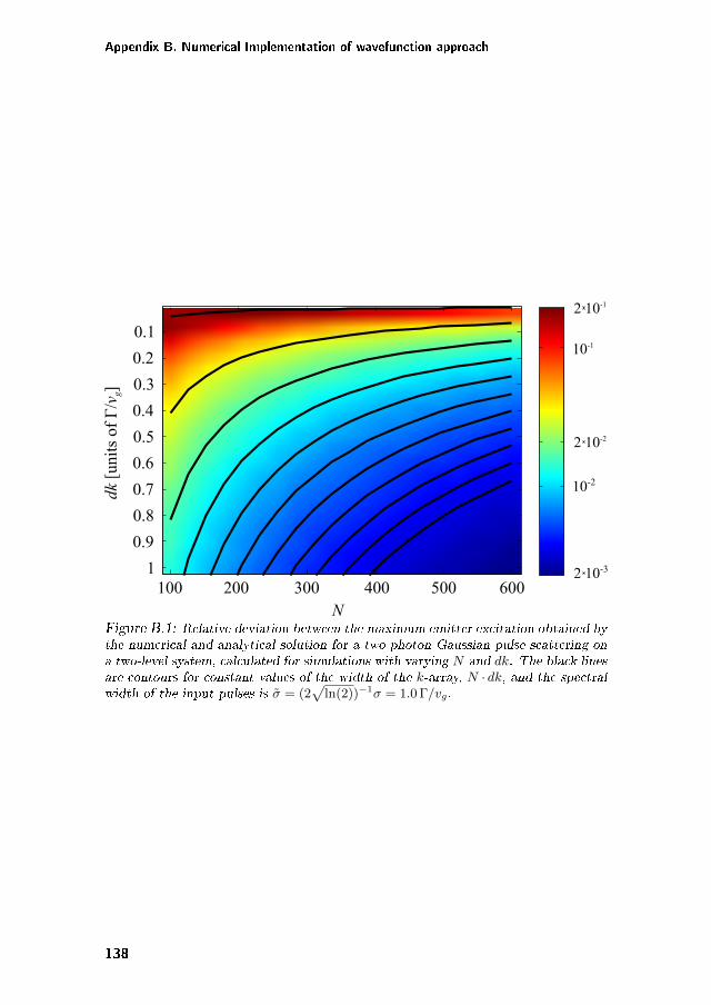
Appendix B. Numerical Implementation of wavefunction approach
10-2
2 10-3
10-1
2 10-1
2 10-2
100 200 300 400 500 600
0.1
0.2
0.3
0.4
0.5
0.6
0.7
0.8
0.9
1
dk
[uni
ts o
f Γ
/vg]
NFigure B.1: Relative deviation between the maximum emitter excitation obtained bythe numerical and analytical solution for a two-photon Gaussian pulse scattering ona two-level system, calculated for simulations with varying 𝑁 and 𝑑𝑘. The black linesare contours for constant values of the width of the 𝑘-array, 𝑁 · 𝑑𝑘, and the spectralwidth of the input pulses is = (2
√ln(2))−1𝜎 = 1.0Γ/𝑣𝑔.
138
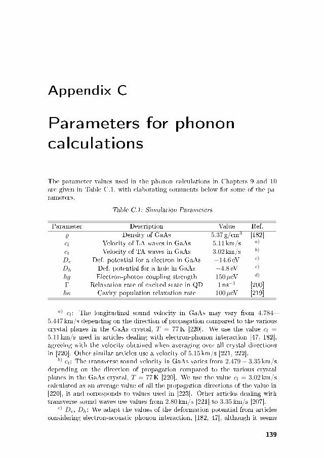
Appendix C
Parameters for phonon
calculations
The parameter values used in the phonon calculations in Chapters 9 and 10are given in Table C.1, with elaborating comments below for some of the pa-rameters.
Table C.1: Simulation Parameters
Parameter Description Value Ref.𝜚 Density of GaAs 5.37 g/cm3 [182]𝑐𝑙 Velocity of LA waves in GaAs 5.11 km/s 𝑎)
𝑐𝑡 Velocity of TA waves in GaAs 3.02 km/s 𝑏)
𝐷𝑒 Def. potential for a electron in GaAs −14.6 eV 𝑐)
𝐷ℎ Def. potential for a hole in GaAs −4.8 eV 𝑐)
~𝑔 Electron-photon coupling strength 150𝜇eV 𝑑)
Γ Relaxation rate of excited state in QD 1 ns−1 [200]~𝜅 Cavity population relaxation rate 100𝜇eV [219]
𝑎) 𝑐𝑙: The longitudinal sound velocity in GaAs may vary from 4.784–5.447 km/s depending on the direction of propagation compared to the variouscrystal planes in the GaAs crystal, 𝑇 = 77K [220]. We use the value 𝑐𝑙 =5.11 km/s used in articles dealing with electron-phonon interaction [47, 182],agreeing with the velocity obtained when averaging over all crystal directionsin [220]. Other similar articles use a velocity of 5.15 km/s [221, 222].
𝑏) 𝑐𝑡: The transverse sound velocity in GaAs varies from 2.479 − 3.35 km/sdepending on the direction of propagation compared to the various crystalplanes in the GaAs crystal, 𝑇 = 77K [220]. We use the value 𝑐𝑙 = 3.02 km/scalculated as an average value of all the propagation directions of the value in[220], it and corresponds to values used in [223]. Other articles dealing withtransverse sound waves use values from 2.80 km/s [221] to 3.35 km/s [207].
𝑐) 𝐷𝑒, 𝐷ℎ: We adapt the values of the deformation potential from articlesconsidering electron-acoustic phonon interaction, [182, 47], although it seems
139
Appendix C. Parameters for phonon calculations
there a big uncertainty in determining agreeing values when measuring thedeformation potentials in different experiments. This is discussed in detail in[202].
𝑑) ~𝑔: For QD in cavities coupling strengths for good cavities have beenshown to be on the order 100 − 200𝜇eV [224, 26]. Thus we pick 𝑔 = 150𝜇eVas a reasonable value.
140
Bibliography
[1] M. Planck. Ueber das Gesetz der Energieverteilung im Normalspectrum.Annalen der Physik, 309(3):553–563, 1901.
[2] A. Einstein. Über einen die Erzeugung und Verwandlung des Lichtes be-treffenden heuristischen Gesichtspunkt. Annalen der Physik, 322(6):132–148, 1905.
[3] T. D. Ladd, F. Jelezko, R. Laflamme, Y. Nakamura, C. Monroe, and J. L.O’Brien. Quantum computers. Nature, 464(7285):45–53, 2010.
[4] C. H. Bennett and G. Brassard. Quantum cryptography: Public key dis-tribution and coin tossing. Proceedings of IEEE International Conferenceon Computers, Systems and Signal Processing, pages 175–179, 1984.
[5] A. K. Ekert. Quantum cryptography based on Bell’s theorem. Phys. Rev.Lett., 67:661–663, 1991.
[6] N. Gisin and R. Thew. Quantum communication. Nat Photon, 1(3):165–171, 2007.
[7] A. Politi, J.C. F. Matthews, and J. L. O’Brien. Shor’s quantum factoringalgorithm on a photonic chip. Science, 325:1221, 2009.
[8] H. J. Kimble. The quantum internet. Nature, 453(7198):1023–1030, 2008.
[9] S. Ritter, C. Nolleke, C. Hahn, A. Reiserer, A. Neuzner, M. Uphoff,M. Mucke, E. Figueroa, J. Bochmann, and G. Rempe. An elemen-tary quantum network of single atoms in optical cavities. Nature,484(7393):195–200, 2012.
[10] J. I. Cirac, P. Zoller, H. J. Kimble, and H. Mabuchi. Quantum statetransfer and entanglement distribution among distant nodes in a quantumnetwork. Phys. Rev. Lett., 78:3221–3224, 1997.
[11] P. Kok, W. J. Munro, K. Nemoto, T. C. Ralph, J. P. Dowling, and G. J.Milburn. Linear optical quantum computing with photonic qubits. Rev.Mod. Phys., 79:135–174, 2007.
[12] W. P. Bowen, N. Treps, R. Schnabel, and P. K. Lam. Experimentaldemonstration of continuous variable polarization entanglement. Phys.Rev. Lett., 89:253601, 2002.
141
BIBLIOGRAPHY
[13] K. Wagner, J. Janousek, V. Delaubert, H. Zou, C. Harb, N. Treps, J. F.Morizur, P. K. Lam, and H. A. Bachor. Entangling the spatial propertiesof laser beams. Science, 321(5888):541–543, 2008.
[14] E. Knill, R. Laflamme, and G. J. Milburn. A scheme for efficient quantumcomputation with linear optics. Nature, 409(6816):46–52, 2001.
[15] C. H. Bennett, G. Brassard, C. Crépeau, R. Jozsa, A. Peres, and W. K.Wootters. Teleporting an unknown quantum state via dual classical andEinstein-Podolsky-Rosen channels. Phys. Rev. Lett., 70:1895–1899, 1993.
[16] J. L. O’Brien, G. J. Pryde, A. G. White, T. C. Ralph, and D. Branning.Demonstration of an all-optical quantum controlled-NOT gate. Nature,426(6964):264–267, 2003.
[17] D. E. Chang, V. Vuletic, and M. D. Lukin. Quantum nonlinear optics –photon by photon. Nat Photon, 8(9):685–694, 2014.
[18] U. Banin, Y. Cao, D. Katz, and O. Millo. Identification of atomic-likeelectronic states in indium arsenide nanocrystal quantum dots. Nature,400(6744):542–544, 1999.
[19] M. Bayer, O. Stern, P. Hawrylak, S. Fafard, and A. Forchel. Hiddensymmetries in the energy levels of excitonic ’artificial atoms’. Nature,405(6789):923–926, 2000.
[20] A. P. Alivisatos. Semiconductor clusters, nanocrystals, and quantumdots. Science, 271(5251):pp. 933–937, 1996.
[21] B. J. M. Hausmann, B. Shields, Q. Quan, P. Maletinsky, M. McCutcheon,J. T. Choy, T. M. Babinec, A. Kubanek, A. Yacoby, M. D. Lukin, andM. Lončar. Integrated diamond networks for quantum nanophotonics.Nano Letters, 12(3):1578–1582, 2012.
[22] A. Faraon, P. E. Barclay, C. Santori, K.-M. C. Fu, and R. G. Beausoleil.Resonant enhancement of the zero-phonon emission from a colour centrein a diamond cavity. Nat Photon, 5(5):301–305, 2011.
[23] M. H. Devoret and R. J. Schoelkopf. Superconducting circuits for quan-tum information: An outlook. Science, 339(6124):1169–1174, 2013.
[24] J.-M. Gérard. Solid-state cavity-quantum electrodynamics with self-assembled quantum dots. In Single Quantum Dots, volume 90 of Topicsin Applied Physics, pages 269–314. Springer Berlin Heidelberg, 2003.
[25] K. M. Birnbaum, A. Boca, R. Miller, A. D. Boozer, T. E. Northup, andH. J. Kimble. Photon blockade in an optical cavity with one trappedatom. Nature, 436(7047):87–90, 2005.
[26] K. Hennessy, A. Badolato, M. Winger, D. Gerace, M. Atature, S. Gulde,S. Falt, E. L. Hu, and A. Imamoglu. Quantum nature of a stronglycoupled single quantum dot-cavity system. Nature, 445(7130):896–899,2007.
142
BIBLIOGRAPHY
[27] D. Englund, A. Faraon, I. Fushman, N. Stoltz, P. Petroff, and J. Vuck-ovic. Controlling cavity reflectivity with a single quantum dot. Nature,450(7171):857–861, 2007.
[28] J. C. F. Matthews, K. Busch. C. F., A. Politi, A. Stefanov, and J. L.O’Brien. Manipulation of multiphoton entanglement in waveguide quan-tum circuits. Nat Photon, 3(6):346–350, 2009.
[29] P. J. Shadbolt, Verde M. R., A. Peruzzo, A. Politi, A. Laing, M. Lobino,J. C. F. Matthews, M. G. Thompson, and J. L. O’Brien. Generating,manipulating and measuring entanglement and mixture with a reconfig-urable photonic circuit. Nat Photon, 6(1):45–49, 2012.
[30] R. Bruck, B. Mills, B. Troia, D. J. Thomson, F. Y. Gardes, Y. Hu, G. Z.Mashanovich, V. M. N. Passaro, G. T. Reed, and O. L. Muskens. Device-level characterization of the flow of light in integrated photonic circuitsusing ultrafast photomodulation spectroscopy. Nat Photon, 9(1):54–60,2015.
[31] F. Priolo, T. Gregorkiewicz, M. Galli, and T. F. Krauss. Silicon nanos-tructures for photonics and photovoltaics. Nat Nano, 9(1):19–32, 2014.
[32] J. Claudon, J. Bleuse, N. S. Malik, M. Bazin, P. Jaffrennou, N. Gregersen,C. Sauvan, P. Lalanne, and J.-M. Gerard. A highly efficient single-photonsource based on a quantum dot in a photonic nanowire. Nat Photon,4(3):174–177, 2010.
[33] P. Yao, V. S. C. Manga Rao, and S. Hughes. On-chip single photonsources using planar photonic crystals and single quantum dots. Laserand Photonics Reviews, 4(4):499–516, 2010.
[34] D. Sahin, A. Gaggero, Z. Zhou, S. Jahanmirinejad, F. Mattioli, R. Leoni,J. Beetz, M. Lermer, M. Kamp, S. Höfling, and A. Fiore. Waveguidephoton-number-resolving detectors for quantum photonic integrated cir-cuits. Applied Physics Letters, 103(11):–, 2013.
[35] R. H. Hadfield. Single-photon detectors for optical quantum informationapplications. Nat Photon, 3(12):696–705, 2009.
[36] G. N. Gol’tsman, O. Okunev, G. Chulkova, A. Lipatov, A. Semenov,K. Smirnov, B. Voronov, A. Dzardanov, C. Williams, and RomanSobolewski. Picosecond superconducting single-photon optical detector.Applied Physics Letters, 79(6):705–707, 2001.
[37] F. Najafi, J. Mower, N. C. Harris, F. Bellei, A. Dane, C. Lee, X. Hu,P. Kharel, F. Marsili, S. Assefa, K. K. Berggren, and D. Englund. On-chipdetection of non-classical light by scalable integration of single-photondetectors. Nat Commun, 6(5873), 2015.
[38] P. Kok and B. W. Lovett. Introduction to Optical Quantum InformationProcessing. Cambridge University Press, 2010.
143
BIBLIOGRAPHY
[39] T. G. Tiecke, J. D. Thompson, N. P. de Leon, L. R. Liu, V. Vuletic, andM. D. Lukin. Nanophotonic quantum phase switch with a single atom.Nature, 508(7495):241–244, 2014.
[40] A. Reiserer, N. Kalb, G. Rempe, and S. Ritter. A quantum gate betweena flying optical photon and a single trapped atom. Nature, 508(7495):237–240, 2014.
[41] W. Chen, K. M. Beck, R. Bücker, M. Gullans, M. D. Lukin, H. Tanji-Suzuki, and V. Vuletić. All-optical switch and transistor gated by onestored photon. Science, 341(6147):768–770, 2013.
[42] H. Kim, R. Bose, T. C. Shen, G. S. Solomon, and E. Waks. A quantumlogic gate between a solid-state quantum bit and a photon. Nat Photon,7(5):373–377, 2013.
[43] D. E. Chang, A. S. Sorensen, E. A. Demler, and M. D. Lukin. A single-photon transistor using nanoscale surface plasmons. Nat Phys, 3(11):807–812, 2007.
[44] T. Volz, A. Reinhard, M. Winger, A. Badolato, K. J. Hennessy, E. L. Hu,and A. Imamoğlu. Ultrafast all-optical switching by single photons. NatPhoton, 6(9):605–609, 2012.
[45] M. Arcari, I. Söllner, A. Javadi, S. Lindskov Hansen, S. Mahmoodian,J. Liu, H. Thyrrestrup, E. H. Lee, J. D. Song, S. Stobbe, and P. Lodahl.Near-unity coupling efficiency of a quantum emitter to a photonic crystalwaveguide. Phys. Rev. Lett., 113:093603, 2014.
[46] S. Ates, Ulrich S. M., A. Ulhaq, S. Reitzenstein, A. Löffler, S. Höfling,A. Forchel, and P. Michler. Non-resonant dot-cavity coupling and itspotential for resonant single-quantum-dot spectroscopy. Nat Photon,3(12):724–728, 2009.
[47] U. Hohenester. Cavity quantum electrodynamics with semiconductorquantum dots: Role of phonon-assisted cavity feeding. Phys. Rev. B,81:155303, 2010.
[48] P. Kaer, T. R. Nielsen, P. Lodahl, A.-P. Jauho, and J. Mørk. Non-Markovian model of photon-assisted dephasing by electron-phonon in-teractions in a coupled quantum-dot–cavity system. Phys. Rev. Lett.,104:157401, 2010.
[49] P. Kaer, P. Lodahl, A.-P. Jauho, and J. Mork. Microscopic theory ofindistinguishable single-photon emission from a quantum dot coupled toa cavity: The role of non-Markovian phonon-induced decoherence. Phys.Rev. B, 87:081308, 2013.
[50] R. Loudon. The Quantum Theory of Light. Oxford University Press,third edition, 2000.
144
BIBLIOGRAPHY
[51] C. Cohen-Tannoudji, J. Dupont-Roc, and G. Grynberg. Photons andAtoms - Introduction to Quantum Electrodynamics. John Wiley and Sons,1989.
[52] W. Schäfer and M. Wegener. Semiconductor Optics and Transport Phe-nomena. Springer-Verlag, 2002.
[53] G. D. Mahan. Many-Particle Physics. Plenum Press, New York, 1990.
[54] P. Kær Nielsen. Fundamental properties of single-photon sources. Mas-ter’s thesis, DTU Fotonik, 2008.
[55] H. Bruus and K. Flensberg. Many-Body Quantum Theory in CondensedMatter Physics. Oxford University Press, 2004.
[56] L. E. Ballentine. Quantum Mechanics - A Modern Development. WorldScientific, 1998.
[57] M. A. Stroscio and M. Dutta. Phonon in Nanostructures. CambridgeUniversity Press, 2004.
[58] C. Kittel. Introduction to Solid State Physics. John Wiley and Sons,eigth edition, 2004.
[59] C. Gerry and P. Knight. Introduction to Quantum Optics. CambridgeUniversity Press, 2005.
[60] S. Stobbe, P. T. Kristensen, J. E. Mortensen, J. M. Hvam, J. Mørk,and P. Lodahl. Spontaneous emission from large quantum dots in nanos-tructures: Exciton-photon interaction beyond the dipole approximation.Phys. Rev. B, 86:085304, 2012.
[61] Q. D. Zhuang, J. M. Li, Y. P. Zeng, L. Pan, H. X. Li, M. Y. Kong,and L. Y. Lin. Structural characterization of InGaAs/GaAs quantumdots superlattice infrared photodetector structures. Journal of CrystalGrowth, 200(3-4):375 – 381, 1999.
[62] A. Goban, C.-L. Hung, S.-P. Yu, J. D. Hood, J.A. Muniz, J.H. Lee, M.J.Martin, A. C. McClung, K. S. Choi, D. E. Chang, O. Painter, and H. J.Kimble. Atom–light interactions in photonic crystals. Nat Commun,5(3808), 2014.
[63] E. Rephaeli and S. Fan. Dissipation in few-photon waveguide transport.Photon. Res., 1(3):110–114, 2013.
[64] Y. Chen, M. Wubs, J. Mørk, and A. F. Koenderink. Coherentsingle-photon absorption by single emitters coupled to one-dimensionalnanophotonic waveguides. New J. Phys., 13(10):103010, 2011.
[65] J. T. Shen and S. Fan. Coherent photon transport from spontaneousemission in one-dimensional waveguides. Opt. Lett., 30(15):2001–2003,2005.
145
BIBLIOGRAPHY
[66] S. Fan, Ş. E. Kocabaş, and J.-T. Shen. Input-output formalism for few-photon transport in one-dimensional nanophotonic waveguides coupledto a qubit. Phys. Rev. A, 82:063821, 2010.
[67] H. Zheng, D. J. Gauthier, and H. U. Baranger. Waveguide QED: Many-body bound-state effects in coherent and Fock-state scattering from atwo-level system. Phys. Rev. A, 82:063816, 2010.
[68] Y. Wu and X. Yang. Strong-coupling theory of periodically driven two-level systems. Phys. Rev. Lett., 98:013601, 2007.
[69] K. J. Blow, R. Loudon, S. J. D. Phoenix, and T. J. Shepherd. Continuumfields in quantum optics. Phys. Rev. A, 42:4102–4114, 1990.
[70] J.-T. Shen and S. Fan. Theory of single-photon transport in a single-modewaveguide. i. coupling to a cavity containing a two-level atom. Phys. Rev.A, 79:023837, 2009.
[71] C. W. Gardiner, A. S. Parkins, and P. Zoller. Wave-function quantumstochastic differential equations and quantum-jump simulation methods.Phys. Rev. A, 46:4363–4381, 1992.
[72] B. Q. Baragiola, R. L. Cook, A. M. Brańczyk, and J. Combes. N-photonwave packets interacting with an arbitrary quantum system. Phys. Rev.A, 86:013811, 2012.
[73] P. Kaer and J. Mørk. Decoherence in semiconductor cavity QED systemsdue to phonon couplings. Phys. Rev. B, 90:035312, 2014.
[74] V. Weisskopf and E. Wigner. Berechnung der natürlichen Linienbreite aufGrund der Diracschen Lichttheorie. Zeitschrift für Physik, 63(1-2):54–73,1930.
[75] G. K. Gulati, B. Srivathsan, B. Chng, A. Cerè, D. Matsukevich, andC. Kurtsiefer. Generation of an exponentially rising single-photon fieldfrom parametric conversion in atoms. Phys. Rev. A, 90:033819, 2014.
[76] M. Keller, B. Lange, K. Hayasaka, W. Lange, and H. Walther. Continu-ous generation of single photons with controlled waveform in an ion-trapcavity system. Nature, 431(7012):1075–1078, 2004.
[77] Y. Chen, T. R. Nielsen, N. Gregersen, P. Lodahl, and J. Mørk. Finite-element modeling of spontaneous emission of a quantum emitter atnanoscale proximity to plasmonic waveguides. Phys. Rev. B, 81:125431,2010.
[78] R. LeVeque. Finite Difference Methods for Ordinary and Partial Differ-ential Equations: Steady-State and Time-Dependent Problems. SIAM,Society for Industrial and Applied Mathematics, 2007.
[79] W. E. Arnoldi. The principle of minimized iterations in the solution of thematrix eigenvalue problem. Quarterly of Applied Mathematics, 9:17–29,1951.
146
BIBLIOGRAPHY
[80] M. Knap, E. Arrigoni, W. von der Linden, and J. H. Cole. Emissioncharacteristics of laser-driven dissipative coupled-cavity systems. Phys.Rev. A, 83:023821, 2011.
[81] W.-B. Yan and H. Fan. Single-photon quantum router with multipleoutput ports. Scientific Reports, 4:4820, 2014.
[82] C. Martens, P. Longo, and K. Busch. Photon transport in one-dimensional systems coupled to three-level quantum impurities. NewJ. Phys., 15(8):083019, 2013.
[83] W.-B. Yan, J.-F. Huang, and H. Fan. Tunable single-photon frequencyconversion in a Sagnac interferometer. Sci. Rep., 3(3555), 2013.
[84] J. Hwang, M. Pototschnig, R. Lettow, G. Zumofen, A. Renn,S. Gotzinger, and V. Sandoghdar. A single-molecule optical transistor.Nature, 460(7251):76–80, 2009.
[85] A. Auffèves-Garnier, C. Simon, J.-M. Gérard, and J.-P. Poizat. Giantoptical nonlinearity induced by a single two-level system interacting witha cavity in the Purcell regime. Phys. Rev. A, 75:053823, 2007.
[86] A. Blais, R.-S. Huang, A. Wallraff, S. M. Girvin, and R. J. Schoelkopf.Cavity quantum electrodynamics for superconducting electrical circuits:An architecture for quantum computation. Phys. Rev. A, 69:062320,2004.
[87] J.-T. Shen and S. Fan. Strongly correlated two-photon transport in aone-dimensional waveguide coupled to a two-level system. Phys. Rev.Lett., 98:153003, 2007.
[88] J.-T. Shen and S. Fan. Strongly correlated multiparticle transport in onedimension through a quantum impurity. Phys. Rev. A, 76:062709, 2007.
[89] T. Shi and C. P. Sun. Lehmann-symanzik-zimmermann reduction ap-proach to multiphoton scattering in coupled-resonator arrays. Phys. Rev.B, 79:205111, 2009.
[90] J.-F. Huang, J.-Q. Liao, and C. P. Sun. Photon blockade induced byatoms with Rydberg coupling. Phys. Rev. A, 87:023822, 2013.
[91] K. Kojima, H. F. Hofmann, S. Takeuchi, and K. Sasaki. Nonlinear in-teraction of two photons with a one-dimensional atom: Spatiotemporalquantum coherence in the emitted field. Phys. Rev. A, 68:013803, 2003.
[92] D. Valente, Y. Li, J. P. Poizat, J M. Gérard, L. C. Kwek, M. F. Santos,and A. Auffèves. Optimal irreversible stimulated emission. New J. Phys.,14(8):083029, 2012.
[93] P. Longo, P. Schmitteckert, and K. Busch. Dynamics of photon transportthrough quantum impurities in dispersion-engineered one-dimensionalsystems. Journal of Optics A: Pure and Applied Optics, 11(11):114009,2009.
147
BIBLIOGRAPHY
[94] P. Longo, P. Schmitteckert, and K. Busch. Few-photon transport in low-dimensional systems. Phys. Rev. A, 83:063828, Jun 2011.
[95] M. Moeferdt, P. Schmitteckert, and K. Busch. Correlated photons inone-dimensional waveguides. Opt. Lett., 38(18):3693–3695, 2013.
[96] D. Witthaut, M. D. Lukin, and A. S. Sørensen. Photon sorters andQND detectors using single photon emitters. EPL (Europhysics Letters),97(5):50007, 2012.
[97] E. Rephaeli and S. Fan. Stimulated emission from a single excited atomin a waveguide. Phys. Rev. Lett., 108:143602, 2012.
[98] C. Cinelli, G. Di Nepi, F. De Martini, M. Barbieri, and P. Mataloni. Para-metric source of two-photon states with a tunable degree of entanglementand mixing: Experimental preparation of Werner states and maximallyentangled mixed states. Phys. Rev. A, 70:022321, 2004.
[99] M. Ostermeyer, D. Korn, D. Puhlmann, C. Henkel, and J. Eisert. Two-dimensional characterization of spatially entangled photon pairs. Journalof Modern Optics, 56(17):1829–1837, 2009.
[100] G. Harder, V. Ansari, B. Brecht, T. Dirmeier, C. Marquardt, and C. Sil-berhorn. An optimized photon pair source for quantum circuits. Opt.Express, 21(12):13975–13985, 2013.
[101] W. P. Grice, A. B. U’Ren, and I. A. Walmsley. Eliminating frequency andspace-time correlations in multiphoton states. Phys. Rev. A, 64:063815,2001.
[102] K. Wang. Quantum theory of two-photon wavepacket interference ina beamsplitter. Journal of Physics B: Atomic, Molecular and OpticalPhysics, 39(18):R293, 2006.
[103] E. Rephaeli, J.-T. Shen, and S. Fan. Full inversion of a two-level atomwith a single-photon pulse in one-dimensional geometries. Phys. Rev. A,82:033804, 2010.
[104] C. K. Hong, Z. Y. Ou, and L. Mandel. Measurement of subpicosecondtime intervals between two photons by interference. Phys. Rev. Lett.,59:2044–2046, 1987.
[105] P. Longo, J. H. Cole, and K. Busch. The Hong-Ou-Mandel effect inthe context of few-photon scattering. Opt. Express, 20(11):12326–12340,2012.
[106] H. Zheng, D. J. Gauthier, and H. U. Baranger. Strongly correlated pho-tons generated by coupling a three- or four-level system to a waveguide.Phys. Rev. A, 85:043832, 2012.
[107] I.-C. Hoi, T. Palomaki, J. Lindkvist, G. Johansson, P. Delsing, and C. M.Wilson. Generation of nonclassical microwave states using an artificialatom in 1d open space. Phys. Rev. Lett., 108:263601, 2012.
148
BIBLIOGRAPHY
[108] G. Vidal and R. F. Werner. Computable measure of entanglement. Phys.Rev. A, 65:032314, 2002.
[109] M. B. Plenio and S. Virmani. An introduction to entanglement measures.Quantum Info. Comput., 7(1):1–51, 2007.
[110] V. Vedral and M. B. Plenio. Entanglement measures and purificationprocedures. Phys. Rev. A, 57:1619–1633, 1998.
[111] H. M. Wiseman and J. A. Vaccaro. Entanglement of indistinguishableparticles shared between two parties. Phys. Rev. Lett., 91:097902, 2003.
[112] G. Ghirardi and L. Marinatto. General criterion for the entanglement oftwo indistinguishable particles. Phys. Rev. A, 70:012109, 2004.
[113] K. Eckert, J. Schliemann, D. Bruss, and M. Lewenstein. Quantum cor-relations in systems of indistinguishable particles. Annals of Physics,299(1):88 – 127, 2002.
[114] R. Paškauskas and L. You. Quantum correlations in two-boson wavefunctions. Phys. Rev. A, 64:042310, 2001.
[115] D. Witthaut and A. S. Sørensen. Photon scattering by a three-levelemitter in a one-dimensional waveguide. New J. Phys., 12(4):043052,2010.
[116] M. Laakso and M. Pletyukhov. Scattering of two photons from two dis-tant qubits: Exact solution. Phys. Rev. Lett., 113:183601, 2014.
[117] T. Shi, S. Fan, and C. P. Sun. Two-photon transport in a waveguidecoupled to a cavity in a two-level system. Phys. Rev. A, 84:063803, 2011.
[118] T. Shi and S. Fan. Two-photon transport through a waveguide coupling toa whispering-gallery resonator containing an atom and photon-blockadeeffect. Phys. Rev. A, 87:063818, 2013.
[119] J.-Q. Liao and C. K. Law. Correlated two-photon transport in a one-dimensional waveguide side-coupled to a nonlinear cavity. Phys. Rev. A,82:053836, 2010.
[120] S. Derouault and M. A. Bouchene. One-photon wave packet interactingwith two separated atoms in a one-dimensional waveguide: Influence ofvirtual photons. Phys. Rev. A, 90:023828, 2014.
[121] A. Nysteen, P. T. Kristensen, D. P. S. McCutcheon, P. Kaer, and J. Mørk.Scattering of two photons on a quantum emitter in a one-dimensionalwaveguide: exact dynamics and induced correlations. New J. Phys.,17(2):023030, 2015.
[122] T. C. Ralph, N. K. Langford, T. B. Bell, and A. G. White. Linear opticalcontrolled-NOT gate in the coincidence basis. Phys. Rev. A, 65:062324,2002.
149
BIBLIOGRAPHY
[123] M. A. Pooley, D. J. P. Ellis, R. B. Patel, A. J. Bennett, K. H. A. Chan,I. Farrer, D. A. Ritchie, and A. J. Shields. Controlled-NOT gate operatingwith single photons. Applied Physics Letters, 100:211103, 2012.
[124] I. Shomroni, S. Rosenblum, Y. Lovsky, O. Bechler, G. Guendelman, andB. Dayan. All-optical routing of single photons by a one-atom switchcontrolled by a single photon. Science, 345(6199):903–906, 2014.
[125] L.-M. Duan and H. J. Kimble. Scalable photonic quantum computationthrough cavity-assisted interactions. Phys. Rev. Lett., 92:127902, 2004.
[126] C. Wang, Y. Zhang, R.-Z. Jiao, and G.-S. Jin. Universal quantum con-trolled phase gate on photonic qubits based on nitrogen vacancy centersand microcavity resonators. Opt. Express, 21(16):19252–19260, 2013.
[127] D. Englund, A. Majumdar, M. Bajcsy, A. Faraon, P. Petroff, andJ. Vučković. Ultrafast photon-photon interaction in a strongly coupledquantum dot-cavity system. Phys. Rev. Lett., 108:093604, 2012.
[128] R. Bose, D. Sridharan, H. Kim, G. S. Solomon, and E. Waks. Low-photon-number optical switching with a single quantum dot coupled toa photonic crystal cavity. Phys. Rev. Lett., 108:227402, 2012.
[129] R. Johne and A. Fiore. Proposal for a two-qubit quantum phase gate forquantum photonic integrated circuits. Phys. Rev. A, 86:063815, 2012.
[130] S. Xu, E. Rephaeli, and S. Fan. Analytic properties of two-photon scat-tering matrix in integrated quantum systems determined by the clusterdecomposition principle. Phys. Rev. Lett., 111:223602, 2013.
[131] M. G. Thompson, A. Politi, J. C. F. Matthews, and J. L. O’Brien. In-tegrated waveguide circuits for optical quantum computing. Circuits,Devices Systems, IET, 5(2):94–102, 2011.
[132] J. Wang, A. Santamato, P. Jiang, D. Bonneau, E. Engin, J. W. Silver-stone, M. Lermer, J. Beetz, M. Kamp, S. Höfling, M. G. Tanner, C. M.Natarajan, R. H. Hadfield, S. N. Dorenbos, V. Zwiller, J. L. O’Brien, andM. G. Thompson. Gallium arsenide (GaAs) quantum photonic waveguidecircuits. Optics Communications, 327:49 – 55, 2014.
[133] A. Martinez, F. Cuesta, and J. Marti. Ultrashort 2-d photonic crystaldirectional couplers. Photonics Technology Letters, IEEE, 15(5):694–696,2003.
[134] T. C. Ralph, I. Söllner, S. Mahmoodian, A. G. White, and P. Lodahl.Photon sorting, efficient bell measurements and a deterministic CZ gateusing a passive two-level nonlinearity. arXiv:1502.04261, 2015.
[135] A. Mohan, P. Gallo, M. Felici, B. Dwir, A. Rudra, J. Faist, and E. Kapon.Record-low inhomogeneous broadening of site-controlled quantum dotsfor nanophotonics. Small, 6(12):1268–1272, 2010.
150
BIBLIOGRAPHY
[136] A. Lyasota, S. Borghardt, C. Jarlov, B. Dwir, P. Gallo, A. Rudra, andE. Kapon. Integration of multiple site-controlled pyramidal quantumdot systems with photonic-crystal membrane cavities. Journal of CrystalGrowth, 414:192 – 195, 2015.
[137] Z. Wang and S. Fan. Optical circulators in two-dimensional magneto-optical photonic crystals. Opt. Lett., 30(15):1989–1991, 2005.
[138] I. Söllner, S. Mahmoodian, S. L. Hansen, L. Midolo, A. Javadi,G. Kiršanske, T. Pregnolato, H. El-Ella, E. H. Lee, J. D. Song, S. Stobbe,and P. Lodahl. Deterministic photon-emitter coupling in chiral photoniccircuits. arXiv:1406.4295, 2015.
[139] K. J. Vahala. Optical microcavities. Nature, 424(6950):839–846, 2003.
[140] D. V. Strekalov, A. S. Kowligy, Y.-P. Huang, and P. Kumar. Progress to-wards interaction-free all-optical devices. Phys. Rev. A, 89:063820, 2014.
[141] Y.-Z. Sun, Y.-P. Huang, and P. Kumar. Photonic nonlinearities via quan-tum Zeno blockade. Phys. Rev. Lett., 110:223901, 2013.
[142] W. M. Itano, D. J. Heinzen, J. J. Bollinger, and D. J. Wineland. QuantumZeno effect. Phys. Rev. A, 41:2295–2300, 1990.
[143] P. N. Butcher and D. Cotter. The Elements of Nonlinear Optics. Cam-bridge University Press, 1990.
[144] T. Tanabe, M. Notomi, H. Taniyama, and E. Kuramochi. Dynamic re-lease of trapped light from an ultrahigh-Q nanocavity via adiabatic fre-quency tuning. Phys. Rev. Lett., 102:043907, 2009.
[145] T.-J. Wang, C.-H. Chu, and C.-Y. Lin. Electro-optically tunable micror-ing resonators on lithium niobate. Opt. Lett., 32(19):2777–2779, 2007.
[146] A. Guarino, G. Poberaj, D. Rezzonico, R. Degl’Innocenti, and P. Gunter.Electro-optically tunable microring resonators in lithium niobate. NatPhoton, 1(7):407–410, 2007.
[147] D. Haertle. Domain patterns for quasi-phase matching in whispering-gallery modes. Journal of Optics, 12(3):035202, 2010.
[148] V. S. Ilchenko, A. A. Savchenkov, A. B. Matsko, and L. Maleki. Nonlinearoptics and crystalline whispering gallery mode cavities. Phys. Rev. Lett.,92:043903, 2004.
[149] Y.-P. Huang and P. Kumar. Interaction-free quantum optical Fredkingates in 𝜒(2) microdisks. Selected Topics in Quantum Electronics, IEEEJournal of, 18(2):600–611, 2012.
[150] A.B. Matsko and V.S. Ilchenko. Optical resonators with whispering-gallery modes-part i: basics. Selected Topics in Quantum Electronics,IEEE Journal of, 12(1):3–14, 2006.
151
BIBLIOGRAPHY
[151] J.-T. Shen and S. Fan. Theory of single-photon transport in a single-mode waveguide. ii. coupling to a whispering-gallery resonator containinga two-level atom. Phys. Rev. A, 79:023838, 2009.
[152] Y.-P. Huang and P. Kumar. Interaction-free all-optical switching in𝜒(2)microdisks for quantum applications. Opt. Lett., 35(14):2376–2378,2010.
[153] D. E. Zelmon, D. L. Small, and D. Jundt. Infrared corrected Sellmeier co-efficients for congruently grown lithium niobate and 5 mol.% magnesiumoxide –doped lithium niobate. J. Opt. Soc. Am. B, 14(12):3319–3322,1997.
[154] J. E. Heebner, T. C. Bond, and J. S. Kallman. Generalized formulationfor performance degradations due to bending and edge scattering loss inmicrodisk resonators. Opt. Express, 15(8):4452–4473, 2007.
[155] G. Nunzi Conti, S. Berneschi, F. Cosi, S. Pelli, S. Soria, G. C. Righini,M. Dispenza, and A. Secchi. Planar coupling to high-Q lithium niobatedisk resonators. Opt. Express, 19(4):3651–3656, 2011.
[156] R. Johne and A. Fiore. Single-photon absorption and dynamic control ofthe exciton energy in a coupled quantum-dot–cavity system. Phys. Rev.A, 84:053850, 2011.
[157] E. E. Hach, A. W. Elshaari, and S. F. Preble. Fully quantum-mechanicaldynamic analysis of single-photon transport in a single-mode waveguidecoupled to a traveling-wave resonator. Phys. Rev. A, 82:063839, 2010.
[158] J. Lin, Y. Xu, Z. Fang, M. Wang, J. Song, N. Wang, L. Qiao, W. Fang,and Y. Cheng. Fabrication of high-Q lithium niobate microresonatorsusing femtosecond laser micromachining. Sci. Rep., 5(8072), 2015.
[159] J. P. Reithmaier, G. Sek, A. Löffler, C. Hofmann, S. Kuhn, S. Reitzen-stein, L. V. Keldysh, V. D. Kulakovskii, T. L. Reinecke, and A. Forchel.Strong coupling in a single quantum dot-semiconductor microcavity sys-tem. Nature, 432(7014):197–200, 2004.
[160] J. M. Gérard, D. Barrier, J. Y. Marzin, R. Kuszelewicz, L. Manin,E. Costard, V. Thierry-Mieg, and T. Rivera. Quantum boxes as activeprobes for photonic microstructures: The pillar microcavity case. AppliedPhysics Letters, 69(4):449–451, 1996.
[161] M. Lermer, N. Gregersen, F. Dunzer, S. Reitzenstein, S. Höfling, J. Mørk,L. Worschech, M. Kamp, and A. Forchel. Bloch-wave engineering of quan-tum dot micropillars for cavity quantum electrodynamics experiments.Phys. Rev. Lett., 108:057402, 2012.
[162] T. Yoshie, A. Scherer, J. Hendrickson, G. Khitrova, H. M. Gibbs, G. Rup-per, C. Ell, O. B. Shchekin, and D. G. Deppe. Vacuum Rabi splittingwith a single quantum dot in a photonic crystal nanocavity. Nature,432(7014):200–203, 2004.
152
BIBLIOGRAPHY
[163] J. Vucković and Y. Yamamoto. Photonic crystal microcavities for cavityquantum electrodynamics with a single quantum dot. Applied PhysicsLetters, 82(15):2374–2376, 2003.
[164] S. Hughes, P. Yao, F. Milde, A. Knorr, D. Dalacu, K. Mnaymneh,V. Sazonova, P. J. Poole, G. C. Aers, J. Lapointe, R. Cheriton, andR. L. Williams. Influence of electron-acoustic phonon scattering on off-resonant cavity feeding within a strongly coupled quantum-dot cavitysystem. Phys. Rev. B, 83:165313, 2011.
[165] A. Majumdar, E. D. Kim, Y. Gong, M. Bajcsy, and J. Vcković. Phononmediated off-resonant quantum dot-cavity coupling under resonant exci-tation of the quantum dot. Phys. Rev. B, 84:085309, 2011.
[166] I. Wilson-Rae and A. Imamoğlu. Quantum dot cavity-QED in the pres-ence of strong electron-phonon interactions. Phys. Rev. B, 65:235311,2002.
[167] E. A. Muljarov and R. Zimmermann. Dephasing in quantum dots:Quadratic coupling to acoustic phonons. Phys. Rev. Lett., 93:237401,2004.
[168] E. M. Gauger, S. C. Benjamin, A. Nazir, and B. W. Lovett. High-fidelityall-optical control of quantum dot spins: Detailed study of the adiabaticapproach. Phys. Rev. B, 77:115322, 2008.
[169] T. B. Norris, J.-K. Rhee, C.-Y. Sung, Y. Arakawa, M. Nishioka, andC. Weisbuch. Time-resolved vacuum rabi oscillations in a semiconductorquantum microcavity. Phys. Rev. B, 50:14663–14666, 1994.
[170] A. Kiraz, M. Atatüre, and A. Imamoğlu. Quantum-dot single-photonsources: Prospects for applications in linear optics quantum-informationprocessing. Phys. Rev. A, 69:032305, 2004.
[171] J. Bylander, I. Robert-Philip, and I. Abram. Interference and correlationof two independent photons. The European Physical Journal D - Atomic,Molecular, Optical and Plasma Physics, 22(2):295–301, 2003.
[172] K. H. Madsen, P. Kaer, A. Kreiner-Møller, S. Stobbe, A. Nysteen,J. Mørk, and P. Lodahl. Measuring the effective phonon density of statesof a quantum dot in cavity quantum electrodynamics. Phys. Rev. B,88:045316, 2013.
[173] P. Kaer, T. R. Nielsen, P. Lodahl, A.-P. Jauho, and J. Mørk. Microscopictheory of phonon-induced effects on semiconductor quantum dot decaydynamics in cavity QED. Phys. Rev. B, 86:085302, 2012.
[174] H.-P. Breuer and F. Petruccione. The Theory of Open Quantum Systems.Oxford University Press, 2002.
[175] H. J. Carmichael. An Open Systems Approach to Quantum Optics.Springer-Verlag, 1993.
153
BIBLIOGRAPHY
[176] H.-P. Breuer, B. Kappler, and F. Petruccione. Stochastic wave-functionmethod for non-Markovian quantum master equations. Phys. Rev. A,59:1633–1643, 1999.
[177] A. Smirne and B. Vacchini. Nakajima-zwanzig versus time-convolutionless master equation for the non-Markovian dynamics of atwo-level system. Phys. Rev. A, 82:022110, 2010.
[178] S. Chaturvedi and F. Shibata. Time-convolutionless projection opera-tor formalism for elimination of fast variables. Applications to Brownianmotion. Zeitschrift für Physik B Condensed Matter, 35(3):297–308, 1979.
[179] G. Lindblad. On the generators of quantum dynamical semigroups. Com-munications in Mathematical Physics, 48(2):119–130, 1976.
[180] L. Jacak, P. Machnikowski, J. Krasnyj, and P. Zoller. Coherent and inco-herent phonon processes in artificial atoms. Eur. Phys. J. D, 22(3):319–331, 2003.
[181] J. Bardeen and W. Shockley. Deformation potentials and mobilities innon-polar crystals. Phys. Rev., 80:72–80, 1950.
[182] B. Krummheuer, V. M. Axt, and T. Kuhn. Theory of pure dephasingand the resulting absorption line shape in semiconductor quantum dots.Phys. Rev. B, 65:195313, 2002.
[183] B. Krummheuer, V. M. Axt, T. Kuhn, I. D’Amico, and F. Rossi. Puredephasing and phonon dynamics in GaAs- and GaN-based quantum dotstructures: Interplay between material parameters and geometry. Phys.Rev. B, 71:235329, 2005.
[184] C. Patel, T. J. Parker, J. Jamshidi, and W. F. Sherman. Phonon fre-quencies in GaAs. Phys. Stat. Sol. (b), 122:461, 1984.
[185] G. Whitfield and P. B. Shaw. Interaction of electrons with acousticphonons via the deformation potential in one dimension. Phys. Rev.B, 14:3346–3355, 1976.
[186] P. Y. Yu and M. Cardona. Fundamentals of Semiconductors. Springer,third edition, 2005.
[187] A. Grodecka, L. Jacak, P. Machnikowski, and K. Roszak. Phonon impacton the coherent control of quantum states in semiconductor quantumdots. arXiv:cond-mat/0404364, 2004.
[188] N. W. Ashcroft and N. D. Mermin. Acoustic Fields and Waves in Solids,Vol II. Krieger, 1989.
[189] M. Esposito and P. Gaspard. Quantum master equation for a systeminfluencing its environment. Phys. Rev. E, 68:066112, 2003.
154
BIBLIOGRAPHY
[190] A. Auffèves, D. Gerace, J.-M. Gérard, M. Fran ça Santos, L. C. Andreani,and J.-P. Poizat. Controlling the dynamics of a coupled atom-cavitysystem by pure dephasing. Phys. Rev. B, 81:245419, 2010.
[191] A. Naesby, T. Suhr, P. T. Kristensen, and J. Mørk. Influence of puredephasing on emission spectra from single photon sources. Phys. Rev. A,78:045802, 2008.
[192] M. S. Kushwaha, P. Halevi, L. Dobrzynski, and B. Djafari-Rouhani.Acoustic band structure of periodic elastic composites. Phys. Rev. Lett.,71:2022–2025, 1993.
[193] B. Krummheuer, V. M. Axt, and T. Kuhn. Coupled polarization andacoustic-phonon dynamics after optical excitation of quantum dots nearsurfaces. Phys. Rev. B, 72:245336, 2005.
[194] M. Maldovan and E. L. Thomas. Simultaneous localization of photonsand phonons in two-dimensional periodic structures. Applied PhysicsLetters, 88:251907, 2006.
[195] A. H. Safavi-Naeini and O. Painter. Design of optomechanical cavitiesand waveguides on a simultaneous bandgap phononic-photonic crystalslab. Opt. Express, 18(14):14926–14943, 2010.
[196] E. Gavartin, R. Braive, I. Sagnes, O. Arcizet, A. Beveratos, T. J.Kippenberg, and I. Robert-Philip. Optomechanical coupling in a two-dimensional photonic crystal defect cavity. Phys. Rev. Lett., 106:203902,2011.
[197] A. Vagov, M. D. Croitoru, V. M. Axt, T. Kuhn, and F. M. Peeters.Nonmonotonic field dependence of damping and reappearance of Rabioscillations in quantum dots. Phys. Rev. Lett., 98:227403, 2007.
[198] S. Weiler, A. Ulhaq, S. M. Ulrich, D. Richter, M. Jetter, P. Michler,C. Roy, and S. Hughes. Phonon-assisted incoherent excitation of a quan-tum dot and its emission properties. Phys. Rev. B, 86:241304, 2012.
[199] A. Wojs, P. Hawrylak, S. Fafard, and L. Jacak. Electronic structure andmagneto-optics of self-assembled quantum dots. Phys. Rev. B, 54:5604–5608, 1996.
[200] S. Stobbe, J. Johansen, P. T. Kristensen, J. M. Hvam, and P. Lo-dahl. Frequency dependence of the radiative decay rate of excitons inself-assembled quantum dots: Experiment and theory. Phys. Rev. B,80:155307, 2009.
[201] R. V. N. Melnik and M. Willatzen. Bandstructures of conical quantumdots with wetting layers. Nanotechnology, 15(1):1, 2004.
[202] I. Vurgaftman, J. R. Meyer, and L. R. Ram-Mohan. Band parametersfor III-V compound semiconductors and their alloys. Journal of AppliedPhysics, 89(11):5815–5875, 2001.
155
BIBLIOGRAPHY
[203] E. T. Jaynes and F. W. Cummings. Comparison of quantum and semiclas-sical radiation theories with application to the beam maser. Proceedingsof the IEEE, 51(1):89–109, 1963.
[204] H. Ezawa. Phonons in a half space. Annals of Physics, 67(2):438 – 460,1971.
[205] M. C. Oliveros and D. R. Tilley. Quantization procedure for phonons inan isotropic elastic half-space. physica status solidi (b), 119(2):675–683,1983.
[206] N. Bannov, V. Mitin, and M. Stroscio. Confined acoustic phonons in afree-standing quantum well and their interaction with electrons. PhysicaStatus Solidi (b), 183(1):131–142, 1994.
[207] N. Bannov, V. Aristov, V. Mitin, and M. A. Stroscio. Electron relaxationtimes due to the deformation-potential interaction of electrons with con-fined acoustic phonons in a free-standing quantum well. Phys. Rev. B,51:9930–9942, 1995.
[208] Y. Y. Liao, Y. N. Chen, W. C. Chou, and D. S. Chuu. Decoherence of acharge qubit embedded inside a suspended phonon cavity. Phys. Rev. B,77:033303, 2008.
[209] W.-M. Ju, K.-D. Zhu, P.-H. Huang, and H. Zheng. The dynamics of adouble-dot charge qubit embedded in a suspended phonon cavity. TheEuropean Physical Journal B, 72(3):417–422, 2009.
[210] Y. Y. Liao and Y. N. Chen. Pure dephasing of double-quantum-dotcharge qubits in freestanding slabs. Phys. Rev. B, 81:153301, 2010.
[211] K. J. Xu and C. Piermarocchi. Dynamics of elastic and inelastic energytransfer between quantum dots in a microcavity. Phys. Rev. B, 84:115316,2011.
[212] A. Nysteen. Cavity QED - engineering the phonon interactions. Master’sthesis, DTU Fotonik, 2011.
[213] Y. Y. Liao, D. S. Chuu, and S. R. Jian. Electric-field-controlled electronrelaxation in lateral double quantum dots embedded in a suspended slab.Journal of Applied Physics, 104:104315, 2008.
[214] P. Borri, W. Langbein, S. Schneider, U. Woggon, R. L. Sellin, D. Ouyang,and D. Bimberg. Ultralong dephasing time in InGaAs quantum dots.Phys. Rev. Lett., 87:157401, 2001.
[215] Charles Santori, David Fattal, Jelena Vuckovic, Glenn S. Solomon, andYoshihisa Yamamoto. Indistinguishable photons from a single-photondevice. Nature, 419(6907):594–597, 2002.
[216] M. Gullans, D. E. Chang, F. H. L. Koppens, F. J. García de Abajo, andM. D. Lukin. Single-photon nonlinear optics with graphene plasmons.Phys. Rev. Lett., 111:247401, 2013.
156
BIBLIOGRAPHY
[217] Y. Yu, M. Heuck, H. Hu, W. Xue, C. Peucheret, Y. Chen, L. K. Oxen-løwe, K. Yvind, and J. Mørk. Fano resonance control in a photonic crystalstructure and its application to ultrafast switching. Applied Physics Let-ters, 105:061117, 2014.
[218] T. P. M. Alegre, A. Safavi-Naeini, M. Winger, and O. Painter. Quasi-two-dimensional optomechanical crystals with a complete phononicbandgap.Opt. Express, 19(6):5658–5669, 2011.
[219] D. Press, S. Götzinger, S. Reitzenstein, C. Hofmann, A. Löffler, M. Kamp,A. Forchel, and Y. Yamamoto. Photon antibunching from a singlequantum-dot-microcavity system in the strong coupling regime. Phys.Rev. Lett., 98:117402, 2007.
[220] J. S. Blakemore. Gallium Arsenide. American Institute of Physics, 1993.
[221] K. Gawarecki, M. Pochwała, A. Grodecka–Grad, and P. Machnikowski.Phonon-assisted relaxation and tunneling in self-assembled quantum dotmolecules. Phys. Rev. B, 81:245312, 2010.
[222] M. Bagheri Harouni, R. Roknizadeh, and M. H. Naderi. Influence ofphonons on exciton-photon interaction and photon statistics of a quan-tum dot. Phys. Rev. B, 79:165304, 2009.
[223] H. Bruus, K. Flensberg, and H. Smith. Magnetoconductivity of quantumwires with elastic and inelastic scattering. Phys. Rev. B, 48:11144–11155,1993.
[224] E. Peter, P. Senellart, D. Martrou, A. Lemaître, J. Hours, J. M. Gérard,and J. Bloch. Exciton-photon strong-coupling regime for a single quan-tum dot embedded in a microcavity. Phys. Rev. Lett., 95:067401, 2005.
157