FETE Complete Illustrative Solutions Fall 2010 1. · FETE Complete Illustrative Solutions Fall 2010 1. ... the weighted average cost of capital is: WACC = (1-rc) ... FETE Fall 2010

FETE Fall 2010 Solutions Page 1

FETE Complete Illustrative Solutions Fall 2010

1. Learning Objectives: 1. Modern Corporate Financial Theory Learning Outcomes: (1b) Calculate the cost of capital for a venture or a firm using the most appropriate

method for given circumstances and justify the choice of method. Sources: Financial Theory and Corporate Policy, Copeland, Weston, Shastri, 4th Edition, 2005, Chapter 15, Pgs. 574 - 578 Commentary on Question: This question was taken straight out of the Copeland and Weston text Chapter 15 (pgs. 576-578) however we changed the numbers. The purpose of this question was to test if the candidates understood the concept of WACC. Many candidates had difficulty with this in prior years. The question required calculations to be performed to allow us to understand if the candidates understood the concept. The expectation was that candidates who understood these concepts would have little difficulty with this question. Most of the candidates did very well on this question. However, for part (c) below, the common error was to forget that cost of equity capital will increase with higher leverage. Had we estimated WACC using old cost of equity capital of 15%, we would have calculated (1-.5)*.06 * .3 + .105*.7 = 8.25% and we would have accepted the project. Solution: (a) Calculate: (i) The company’s current weighted average cost of capital.

Using CAPM: kt = Rf + [E(Rm) - Rf]BL =.06 + [.15 - .06] x .5 = 10.50% Therefore, the weighted average cost of capital is: WACC = (1-rc)Rf B/(b+S) + ks S/(b+S) = (1 -0.5) x 0.06 x 0.15 + 0.1050 x 0.85 = 9.375%


1. Continued

OR Using M-M: WACC = p(1 - tc B/(B + S)) p = Rf + [E(Rm) - Rf]BU BU = BL/(1+(1-tc) B/S) =.5/(1+(1-.5)*.15/.85) = .45946 p=.06 + [.15 - .06] x .4595 = 10.136% WAC = .10136*(1-.5*.15) = 9.38%

(ii) The current cost of equity.

Using CAPM: ks = Rf + [E(Rm) - Rf]BL =.06 + [.15 - .06] x .5 = 10.50% OR Using M-M: ks = p + (1-tc)(p - Rf)B/S p = Rf + [E(Rm) - Rf]BU BU = BL/(1+(1-tc) B/S) =.5/(1+(1-.5)*.15/.85) = .45946 p=.06 + [.15 - .06] x .4595 = 10.136% ks = .1014 + .5*(.1014 - .06)*(.15/.85) = .1050

(b) Calculate the new weighted average cost of capital.

Using CAPM: WACC = (1-tc)Rf B/(B+S) + ks S/(B+S) ks = kf + new Bl x (Rm-Rf) BU = BL / (1 + (1 - tc) x (B / S) ) = = 50% / (1 + 0.5 * 15%/85%) = 45.95% BL = (1+(1-tc) x (B/S)) x BU = (1 + 50% x 30%/70%) x 45.95% = 55.8% ks = .06 + [.15 - .06] x .558 = 11.02% WACC=(1-.5) x 0.06 x (0.3) + 0.1102 x 0.7 = 8.61%


1. Continued OR Using M-M: WACC = p(1 - tc B/(B + S)) This assumes p calculated in 1a. If not: p = Rf + [E(Rm) - Rf]BU BU = BL/(1+(1-tc) B/S) =.5/(1+(1-.5)*.15/.85) = .45946 p=.06 + [.15 - .06] x .4595 = 10.136% WACC = 10.14% x [ 1 - .5 x .3 ] = 8.61%

(c) Recommend whether or not the company should invest in the project, and justify your recommendation.

Since 8.50% < 8.61% The new project with its 8.5% rate of return will not be acceptable even if the firm increases its debt to total assets from 15% to 30%. Need to incorporate higher cost of equity capital due to higher leverage.


2. Learning Objectives: 1. Modern Corporate Financial Theory Learning Outcomes: (1h) Recommend a specific legal form of organization and justify the choices. (1j) Identify sources of agency costs and explain methods to address them. Sources: FET-162-08: Financial Markets and Corporate Strategy, Grinblatt & Titman, 2nd Edition, Ch. 18, How Managerial Incentives Affect Financial Decisions FET-166-09: Megginson, W. L., Corporate Finance Tehory, Ch. 2, “Ownership, Control and Compensation” Commentary on Question: The question was derived from study notes FET 162-08 and FET 166-09. This question was about half recall and half comprehension. This question covers learning outcomes (1h), and (1j) which have rarely been tested. The performance of the candidates on this question was very good. Candidates generally did well on part (a). A common mistake was to reverse the advantages of S-Corp and C-Corp. Some candidates did not justify the recommendation. Also many candidates discussed tax advantages in the recommendation but did not list it in the advantages. Part (b)(i) was generally answered well and for (b)(ii) the question asked for a list, but candidates generally focused on 3 big categories without any further elaboration. For part (b)(iii) most of the candidates gave internal mechanisms rather than external so they did not do well. Note that the answer below shows all the pieces that were acceptable, however it only took slightly less than half of the bullet points below to receive full credit. Solution: (a) For this venture that you plan on undertaking: (i) List the advantages and disadvantages of choosing each of the forms.

1. Partnership Advantages: No legal distinction – each can execute contracts Partnership income is taxed only once, at the personal level Allows a large number of people to pool expertise and capital


2. Continued Partnerships are competitive in knowledge intensive business – which is the type of business an actuarial firm would be Business isn’t automatically terminated following the death or retirement of a partner if there is a partnership agreement Cheaper to establish (compared to corporations) Disadvantages: Limited life Limited access to capital (restricted to retained profits and personal borrowings); cannot do an IPO Unlimited personal liability – they are not willing to lose personal property No legal distinction – each can execute contracts, but each is personally liable for all debts of the partnership

2. Limited Partnership Advantages: Allows a large number of people to pool expertise and capital Partnerships are competitive in knowledge intensive business – which is the type of business an actuarial firm would be Business isn’t automatically terminated following the death or retirement of a partner if is a partnership agreement Partnership income is taxed only once, at the personal level Cheaper to establish (compared to corporations) Disadvantages: Costly to establish Difficult to monitor the general partner Illiquid Limited access to capital (restricted to retained profits and personal borrowings); cannot do an IPO At least one partner must have unlimited liability – nobody is willing to lose personal property

3. S-corporation Advantages: Taxed as partners – once, at personal level Limited liability Flexible – can easily become a C-corp once the 35 shareholder ceiling is crossed Perpetual life feature – can prosper for many generations Separate economic entity – can contract individually with managers, suppliers, customers, etc


2. Continued

Disadvantages: Restricted financing - can only have a single class of equity outstanding High transaction costs Expensive to create Most states levy annual corporate charter taxes Listing fees Reporting expenses with SEC e.g. printing, mailing, legal, auditing 4. C-corporation Advantages: Limited liability Perpetual life feature – can prosper for many generations Separate economic entity – can contract individually with managers, suppliers, customers, etc Stable / has lots of access to capital; can issue securities, borrow money from creditors, issue stock Ownership structure can be continually changed Disadvantages: Taxed twice, at personal and company level; there’s concern over after-tax profits High transaction costs Expensive to create Most states levy annual corporate charter taxes Listing fees Reporting expenses with SEC e.g. printing, mailing, legal, auditing Governance problems (if they eventually become big enough) Separation of ownership and control – interests between managers and shareholders are usually not aligned Collective action problem (if they eventually become big enough) Best interest of group for action to be taken (to monitor and discipline management), but it is in no individual group member’s rational self interest to precipitate action


2. Continued

(ii) Recommend and justify which form you should choose.

S-corp They are only seven (meet the 35 max ceiling requirement) Limited liability Taxed only once In Limited Partnership, passive partners cannot have an active role Can easily convert an S-corp into a C-corp if the venture is successful (IPO)

(b)

(i) Describe potential conflicts of interest with your older family members as shareholders of the company that you and your college friends may have from investing the assets of the firm.

You and your college friends (as managers) may choose to: 1. Make investments that fit their own expertise so that they become

invaluable If desire to remain on the job is large Difficult to replace in the future Rely on implicit contracts & personal relationships in their business dealings, making it more difficult for potential replacements to complete the deals they initiate/private consumption/diversion of resources

2. Different time horizons

Make investments that pay off early, even when they hurt in the long run Having favorable financial results in the short run may allow managers to raise capital at more favorable rates

3. Different risk tolerances, e.g.

Make investments that minimize the manager’s risk Increase the scope of the firm to reduce chances of bankruptcy, even when it is suboptimal (i.e. they expand faster than they should) Increase scope of firm to increase their compensation, even when it is suboptimal Make investments that are too conservative, not value-maximizing to reduce chance of bankruptcy


2. Continued

(ii) List and explain ways in which compensation for you and your college friends may be designed to better align your interests with the interests of your older family members as shareholders of the company.

1. Cash bonus

Reward if business unit performance exceeds a certain level

2. Stock options Right to purchase stock at a fixed price, for a given number of years expires value-less if stock price doesn’t rise high enough to make the options in the money

3. Deferred cash or stock options/ golden handcuffs Payment received if he or she remains with the company for a given period of time they raise the price a competitor has to pay to entice one of a firm’s best employees

4. Golden parachute Cash payment made if executive loses their job; minimizes oppositions to takeovers that would be beneficial to stakeholders

5. Stock appreciation right / phantom stock / align interests w/shareholders/ share based compensation Give managers cash payments that mirror those received by shareholders Minimizes stock ownership dilution

6. Relative performance contract Determine compensation according to how well the executive’s firm performs relative to some benchmark Eliminates risks that are beyond the manager’s control

7. Earnings based compensation

(iii) Explain other external mechanisms that can be used as a means of corporate governance for the organization.

1. Disciplinary takeovers from another organization; crude but effective 2. Rise in power and assertiveness of institutional investors, i.e. the older

family members Oppose management-sponsored takeover defense initiatives/ proxy fights Challenge unwarranted grants of stock options/executive perks Demanding performance from poorly performing management teams


3. Learning Objectives: 1. Modern Corporate Financial Theory 5. Efficient Markets & Information Theory Learning Outcomes: (1c) Evaluate various profitability measures including IRR, NPV and ROE, etc. (5a) Define capital market efficiency and the value of information. Sources: Financial Theory and Corporate Policy, Copeland, Chapter 2, pgs. 27-28 and Chapter 10 pgs. 355-359 Commentary on Question: This was an application question. The purpose of this question was to demonstrate an understanding of the value of information. The value of information is a critical component in the concept of capital market efficiency. The candidates did very well on this question overall. However, areas where the candidates did poorly were: Overall: Not appropriately reflecting capital requirements (i.e. time value of money) In part (a): Not rejecting the risks appropriately In part (b): Not reflecting the full period of the license Solution: (a) Calculate the value of the information provided by the software on each contract

underwritten.

V( No prediction (probability 50%) Test provides no predictive value Value = 1 (same as V( Bad risk (probability 25%) Probability Value 0 5 0.5 1 0.5 -3 Expected value of a bad risk = 0 * 5 + 0.5 * 1 + 0.5 * (-3) = -1 We should reject the bad risk


3. Continued

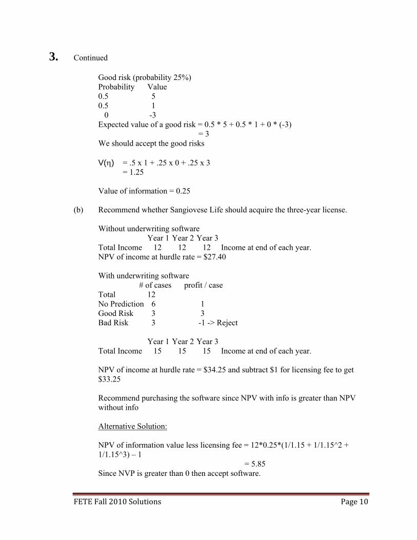
Good risk (probability 25%) Probability Value 0.5 5 0.5 1 0 -3 Expected value of a good risk = 0.5 * 5 + 0.5 * 1 + 0 * (-3) = 3 We should accept the good risks V() = .5 x 1 + .25 x 0 + .25 x 3 = 1.25 Value of information = 0.25

(b) Recommend whether Sangiovese Life should acquire the three-year license.

Without underwriting software Year 1 Year 2 Year 3 Total Income 12 12 12 Income at end of each year. NPV of income at hurdle rate = $27.40 With underwriting software # of cases profit / case Total 12 No Prediction 6 1 Good Risk 3 3 Bad Risk 3 -1 -> Reject Year 1 Year 2 Year 3 Total Income 15 15 15 Income at end of each year. NPV of income at hurdle rate = $34.25 and subtract $1 for licensing fee to get $33.25 Recommend purchasing the software since NPV with info is greater than NPV without info Alternative Solution: NPV of information value less licensing fee = 12*0.25*(1/1.15 + 1/1.15^2 + 1/1.15^3) – 1 = 5.85 Since NVP is greater than 0 then accept software.


4. Learning Objectives: 2. Corporate Financial Applications Learning Outcomes: (2e) Apply real options analysis to recommend and evaluate firm decisions on capital

utilization. Sources: Copeland, Weston, Shastri, Financial Theory and Corporate Policy, 4th Edition, Ch. 9: Multi-period Capital Budgeting under Uncertainty: Real Options Analysis Commentary on Question: This question asked candidates to state the three common assumptions used in real options and then apply their understanding towards a calculation of the value of a project for an option to expand. Overall, most candidates understood what was required of them to earn most of the credit for this question. For part (a), many candidates listed the 3 assumptions, but did not describe the main components of each, which was required to earn full credit. Also, a small number of candidates listed MAD but did not expand this to “Marketed Asset Disclaimer.” For part (b), several candidates did not round this figure as directed in the question. For part (c), several candidates did not indicate whether it would be optimal to exercise the option, which would have demonstrated the level of analysis expected for this part of the question. Candidates were not expected to determine whether to exercise the option once it was already determined to be optimal at node H but were not penalized for this additional step. Candidates were generally split in terms of whether they used discrete or continuous discounting, and although the discrete method would have been preferred, candidates were not penalized for using this approach. Solution: (a) Describe all assumptions that you will use to price this real option.

Assumption 1 MAD – marketed asset disclaimer Can use the present value of the project (assuming no flexibility to make future decisions) as a twin security


4. Continued

Assumption 2 No arbitrage assumption Replicating portfolio correctly values the real option contingent on the underlying Assumption 3 Regardless of the pattern of expected cash flows, we can use recombining binomial trees to model the evolution of a project over time Properly anticipated prices fluctuate randomly/random walk

(b) Calculate q, the risk neutral probability, to two decimal places.

To calculate the value of the project with the option, we need to calculate q, or the risk-neutral probability, calculated as:

q = (1 + rf – d)/(u – d) = (1 + 0.048 – 1/1.2) / (1.2 – 1/1.2) ~ 0.59 (rounded to 2 decimal places)

(c) Calculate each of the following, assuming the expansion option is available at

each future stage of the project: (i) The value at each future stage

At each node of the new tree (below), the value of the project is calculated as:

Value = Max (Value x 1.3 – 110, Value without expanding)

H

F

I V0‘ = ? G

J


4. Continued

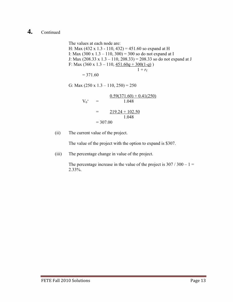
The values at each node are: H: Max (432 x 1.3 - 110, 432) = 451.60 so expand at H I: Max (300 x 1.3 – 110, 300) = 300 so do not expand at I J: Max (208.33 x 1.3 – 110, 208.33) = 208.33 so do not expand at J F: Max (360 x 1.3 – 110, 451.60q + 300(1-q) ) 1 + rf

= 371.60

G: Max (250 x 1.3 – 110, 250) = 250 0.59(371.60) + 0.41(250) V0‘ = 1.048

= 219.24 + 102.50 1.048 = 307.00

(ii) The current value of the project.

The value of the project with the option to expand is $307.

(iii) The percentage change in value of the project.

The percentage increase in the value of the project is 307 / 300 – 1 = 2.33%.


5. Learning Objectives: 2. Corporate Financial Applications Learning Outcomes: (2f) Describe the process, methods and effects of a potential acquisition or reinsurance

of a business including its effect on capital structure, return on equity, price/earnings multiples and share price.

Sources: FET-151-08: “Real and Illusory Value Creation by Insurance Companies,” D. Babbel and C. Merrill, Journal of Risk and Insurance, 2005, Vol. 72, No.1, 1-21 FET-161-08: Tiller & Tiller, Life, Health and Annuity Reinsurance, Ch. 5: Advanced Methods of Reinsurance Commentary on Question: This question asks the candidate to structure a funds-withheld or modified coinsurance deal, with particular attention to the capital management effects of the structure. This situation frequently occurs in practice when companies seek to manage products with heavy capital strain that are selling well, such as universal life with secondary (no-lapse) guarantees. The candidates tended to do well on parts (a) and (b). For part (c), see note in italics. Candidate responses were mixed. Solution: (a) List reasons for maintaining assets with the ceding company in a reinsurance

structure.

Larger sums create concern for the reserve security and reinsurance credit worthiness.

Initial transaction frequently involves the transfer of assets that match the liabilities rather than cash. Leaving the assets with the ceding company allows the reinsurer to take advantage of the favorable existing portfolio without incurring capital gains and losses.

Transfer of ownership of assets or selling assets for cash may create unnecessary and untimely capital gains and losses for the ceding company, creating statutory capital and tax issues.

Given the short timeframe for execution of most transactions, it may be unfeasible to purchase the volume of assets needed if cash were used.

Potential Recapture at a later date is more easily accomplished if the assets stay with the ceding company.

If ceding company retains a percentage of business, it may be advantageous to leave all the assets for the underlying business in a single portfolio, aligning the ceding company’s and reinsurer’s views of credited and earned rates.

The ceding company may want to continue to manage the assets for a fee..


5. Continued (b) Evaluate the advantages and disadvantages to Rioja of the approach in (a).

Identify approach is Modified Coinsurance.

Advantages Applicable to all plans of insurance Ceding company avoids the necessity of liquidating or transferring ownership

of assets to the reinsurer when an inforce block is involved Allows the ceding company to retain control of the investment policy for the

block of business (especially good for PAR) Modified Coinsurance eliminates the reserve credit problem found in

coinsurance if the reinsurer is not licensed in the ceding company’s state of domicile

Reinsurer may prefer Modified Coinsurance to avoid the necessity of managing assets

Disadvantages Some find it complicated to administer because of the Modified Coinsurance

adjustment Special transactions are required in the case of surrenders and death Transfer of assets back to the reinsurer in the event of treaty termination can

create exposure to capital losses for the ceding company Transfer of the initial Modification Coinsurance adjustment to the ceding

company can create problems for the reinsurer (c) Calculate the coinsurance percentage (%) required such that the free surplus set

aside is adequate to support sales for one year.

This may be solved in a variety of ways: The candidate should either explicitly or implicitly identify the following:

Gain From Operations + Surplus = 0 Note: Full marks were given for clear set up of this formula either in a table or algebraic form. Many candidates made the mistake of setting the formula as Gain From Operations = Surplus Extending the above formula and recognizing that the change in inforce reserve is offset by investment income (based on the information provided that Actual investment income is as expected) and that ceded entries are offset by a Modified Coinsurance adjustment the following formula is derived: Prem*coins +Res(t-1)*Allow*Coins +Prem*Allow*coins+Prem*Coins-ResChgNB+ResChgInf+expenses-Surplus=0


5. Continued

Then solving for the coinsurance % coins=(ResChgNB+Expenses-Surplus-Prem)/(Res(t-1)*Allow +Prem*Allow+ResCHgNB-Prem) Providing an answer of 23%

(d) Describe conditions which should be included in a treaty in order to gain

acceptance by the regulators in Rioja’s country of domicile.

The reinsurer must have an actual obligation to pay benefits should experience reach a certain level.

Gains to the reinsurer must be based on the actual experience of the reinsurance.

No event, such as insolvency or management change, should automatically terminate the reinsurance in force. However, reinsurance may be terminated due to a certain level of earnings being attained or if a warranty is violated.

Inforce reinsurance cannot be terminated unilaterally by the reinsurer, except for nonpayment of premiums.

Interest paid or credited via the reinsurance should be reasonable in relation to the investment markets of the assets involved.

The ceding company should not be forced to pay back losses except for voluntary termination.

The relevant significant risks of the underlying policies should be transferred to the reinsurer if they are deemed relevant including: The candidate could have attained additional credit for listing risks that could be deemed significant such as: - Capital loss - Disintermediation - Asset default risks


6. Learning Objectives: 3. Derivatives and Pricing Learning Outcomes: (3a) Define the cash flow characteristics of complex derivatives including exotic

options, interest rate derivatives, swaps and other non-traditional derivatives. Sources: Hull, J.C., Options Futures & Other Derivatives, 7th Edition, 2008 Ch. 19: Basic Numerical Procedures Ch. 24: Exotic Options Ch. 26: More on Models and Numerical Procedures (26.1, 26.2, 26.3 only) Commentary on Question: This question tested the pricing an exotic option involving asset exchange. The candidates needed to demonstrate they knew how the price is affected by (i) the presence of storage cost, and (ii) the change in correlation coefficient between the two underlying assets Most candidates did not get that the option value at time 0 is U0 e

-quT + V0 e-qv T N(d1) -

U0 e-quT N(d2).

Instead many candidates derived the option value at time 0 using U0 + V0 e

-qv T N(d1) - U0 e

-quT N(d2), which is only right when assuming qu = 0. In general part (b)(i) was very straight forward and the candidates did well. Some common mistakes included: Only calculating the value of the exchange option in part (b)(i), but did not give the

final value of the contract Using 1600 and 1250 as initial value, rather than 4800 and 5000 Used 4Su and 3Sv instead of Su and Sv In part (b)(ii), most candidates knew that storage cost is similar to dividend, but only a few candidates knew that it’s actually negative (i.e.: qu < 0, qv < 0 ). Many candidates discuss the effects of storage cost in terms of e-quT, but very few candidates discussed how the relative value of qu, qv affects N(d1) and N(d2). In general, candidates did very well in part (c). Solution: (a) Derive the value of this contract at issue; define all symbols.

The value of option at expiration is given as max(UT, VT) It can be written as UT + max(VT - UT, 0) The option max(VT - UT, 0) has a value only if VT > UT , where subscript implies values are at time T


6. Continued The option value at time 0 is e-rT E(UT)+ V0 e

-qv T N(d1) - U0 e-quT N(d2)

where E(UT) is the expected value of UT in a risk neutral world but E(UT) = e(r - qu)T U0 Therefore the option value at time 0 is U0 e

-quT + V0 e-qv T N(d1) - U0 e

-quT N(d2) d1 =[ ln(V0/U0) + (qu - qv + s2/2)T ] / (sT0.5), d2 = d1 - sT0.5

s2 = su2 + sv

2 - 2ρ su sv where U0, V0 are the assets prices at time 0, qu, qv are the dividend yield of assets U and V respectively su and sv are volatilities of U and V, respectively, and ρ is the correlation coefficient

(b)

(i) Calculate the price of a 1-year European option which pays the price of 4 ounces of gold or 3 ounces of platinum, whichever is greater.

Assume U=gold, V=platinum, Inputs are U0 = 4*1250 = 5000, V0 = 3*1600 = 4800, T = 1, qu = qv = 0, su = 0.2, sv = 0.25, ρ = 0.7 s2 = su

2 + sv2 - 2ρ su sv = 0.22 + 0.252 - 2*0.7*0.2*0.25 = 0.0325

s = 0.1803 d1 =[ ln(4800/5000) + 0.0325/2 ] / 0.18028 = -0.1363 d2 = -0.1363 - 0.1803 = -0.3166 N(d1) = 0.4458, N(d2) = 0.3758 f0 = 4800*0.4458 - 5000*0.3758 = 260.84 option price = 5000 + 260.84 = 5260.84 OR Could have also assumed U=platinum V=gold, Then inputs are U0 = 3*1600 = 4800, V0 = 4*1250 = 5000, d1 =[ ln(5000/4800) + 0.0325/2 ] / 0.18028 = 0.3166 d2 = 0.3166 - 0.1803 = 0.1363 N(d1) = 0.6242, N(d2) = 0.5542 \f0 = 5000*0.6242 - 4800*0.5542 = 460.84 \option price = 4800 + 460.84 = 5260.84

(ii) Describe the effect on the option price if the assets require storage at non-

zero cost (without further calculation).

If storage costs exist then qu < 0, qv < 0 . Storage cost is essentially a negative dividend yield. The option value = U0 e

-quT + V0 e-qv T N(d1) - U0 e

-quT N(d2) Therefore option value will increase by a factor of e-quT.if qu=qv.


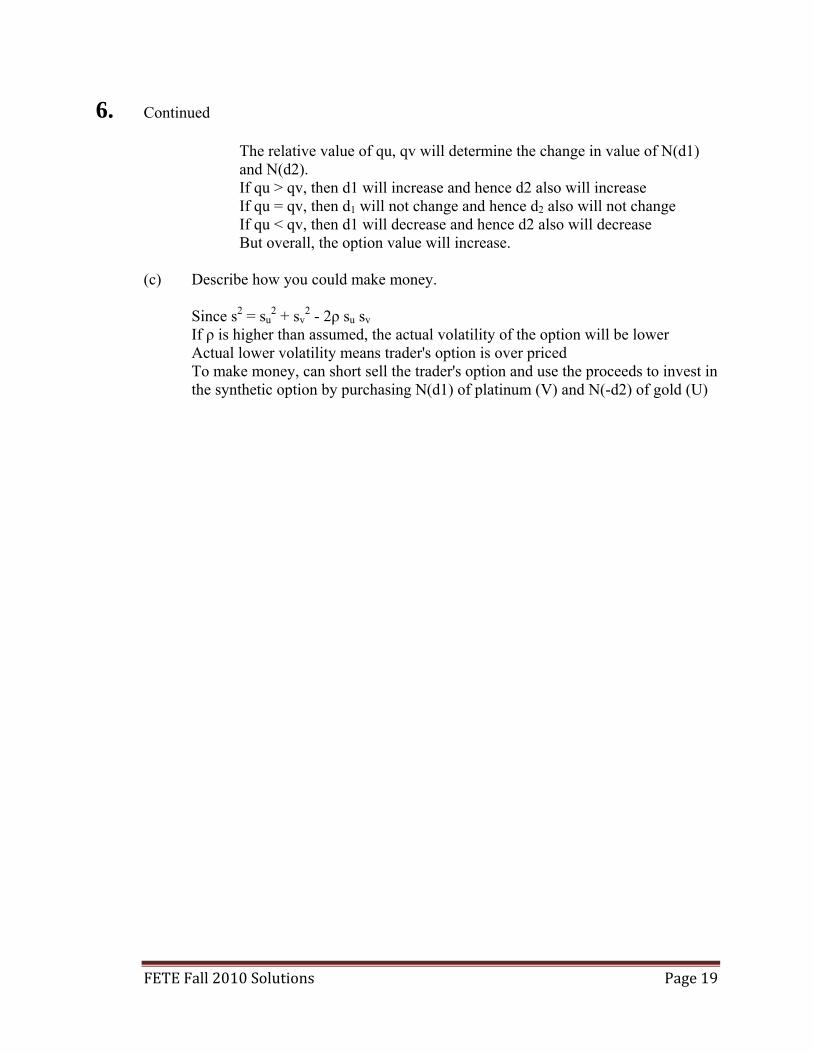
6. Continued The relative value of qu, qv will determine the change in value of N(d1) and N(d2). If qu > qv, then d1 will increase and hence d2 also will increase If qu = qv, then d1 will not change and hence d2 also will not change If qu < qv, then d1 will decrease and hence d2 also will decrease But overall, the option value will increase.

(c) Describe how you could make money.

Since s2 = su

2 + sv2 - 2ρ su sv

If ρ is higher than assumed, the actual volatility of the option will be lower Actual lower volatility means trader's option is over priced To make money, can short sell the trader's option and use the proceeds to invest in the synthetic option by purchasing N(d1) of platinum (V) and N(-d2) of gold (U)


7. Learning Objectives: 3. Derivatives and Pricing Learning Outcomes: (3b) Evaluate the risk/return characteristics of complex derivatives. Sources: Hull, J.C., Options Futures & Other Derivatives, 7th Edition, 2008 Ch. 7: Swaps Commentary on Question: The question tested the candidates’ knowledge of an interest rate swap transaction and also the correct theoretical valuation of the swap after issue. The question also demanded the candidates understand the interest rate swap transaction and whether or not it would be an effective asset liability management tool. For part (a), few candidates received full credit for this part. Frequently answers were vague and didn't provide sufficient explanation of a company borrowing where it has comparative advantage (e.g., floating) and then swapping to pay the kind of rate (e.g., fixed) that it really wants. Also, some candidates did not answer the question as asked but answered based on currency swaps (sometimes points could be awarded, though). For part (b), many candidates received full credit. A common error, however, was assuming that the gain from the swap had to be split evenly, and so an incorrect swap fixed rate or incorrect swap floating rate (or both) would be used to force an evenly split gain. A diagram of the transactions would have been helpful but was not necessary for full credit. Partial credit was awarded for correctly calculating total gain even if the answer was otherwise incorrect. It was not uncommon for candidates to get the net effect correct for each party but then not calculate rate reduction for each company (as asked in the question). For part (c), the reading provides two approaches to valuing the swap. One of them, using a forward rate agreement approach, is untenable because it requires knowing the actual 6-month LIBOR rate at the valuation date and that information is not provided. The appropriate valuation approach is “Valuation in Term of Bond Prices.” Nearly every candidate failed to recognize that the value of the floating piece of the swap was equal to the notional at the valuation date (and so required no calculations). Few understood how to use the swap rate to determine the 2-yr zero rate, which is needed for correct discounting. Also, a common error in valuing B(fix) was to not use the fixed rate of the swap entered into (i.e., 7.68%) as the fixed payment, but instead use the swap rate (or bid rate or offer rate) at the valuation date. Most candidates knew that the V(swap) = B(float) – B(fix) , and most candidates demonstrated correctly how to use the result of the V(swap) as calculated.


7. Continued Solution: (a) Describe and critique the Comparative Advantage argument to explain the

popularity of interest rate swaps in capital financing.

The argument is called the comparative-advantage argument. Some companies have a comparative advantage when borrowing in fixed-rate markets. Others have a comparative advantage in floating rate markets. To obtain a new loan, it makes sense for a company to go to the market where it has a comparative advantage. As a result, the company may borrow floating (fixed) when it wants fixed (floating). A swap is then used to transform a fixed (floating) rate loan into a floating (fixed) rate loan. Criticism: The terms of floating rates bonds are likely to be renegotiated in the event that a credit rating downgrade occurs. In this way, the company paying the fixed rate in the swap doesn’t necessarily lock in their cost of funds.

(b) Show that a swap rate of 7.36% between Malbec and Valpolicella would lower

the borrowing costs for both companies, and calculate the rate reduction for each company.

Malbec should borrow fixed at 8.00% because it has comparative advantage (CA) at fixed rate

Enter into a swap to receive fixed at 7.36% Pay floating rate of LIBOR (=L) Malbec’s net financing cost is to pay floating = 8.00% - 7.36% + L = L + 0.64%

Malbec’s rate reduction using swap = Usual floating borrowing cost – Floating cost w/ swap = (L + 1.30%) – (L + 0.64%) = 0.66% Valpolicella should borrow floating at L + 1.91% because it has CA at floating rate

Enter into a swap to pay fixed 7.36%, and Receive floating of L Valpolicella’s net financing cost is to pay fixed = L + 1.91% +7.36% - L = 9.27%

Valpolicella’s rate reduction using swap = Usual fixed borrowing cost – Fixed cost w/ swap = 9.70% - 9.27% = 0.43% (Note, as a check: 0.66% + 0.43% = 1.09% = (9.70% - 8.00%) – [(L+1.91%) – (L+1.30%)].)


7. Continued (c) Evaluate whether or not the swap has proved to be an effective asset liability

management tool for Valpolicella.

The swap is effective if the gain in the swap offsets the loss in the project. Gain in swap = (value of swap at t=1) – (value of swap at t=0) At time 0, the V(swap) = 0. At time 1, B(Floating) = Notional = 10,000,000 , because a payment was just made At time 1, B(Fix) = discounting of remaining 4 fixed payments Need 2 yr zero rate to value B(Fix): The two year swap rate is the average of the bid and offer rates, 8.17% = (8.15% + 8.19%)/2 The two year swap rate is equal to the two year par yield, thus, for 100 notional, 4.085*[e^(-.5*7.9%) + e^(-1*8%) + e^(-1.5*8.1%)] + 104.085*e^(-2*2 yr zero) = 100 So 2 yr zero = 8.01%

At time 1, B(Fix) = 10,000,000*[3.68% (e^(-.5*7.9%)+e^(-1*8.0%)+e^(-1.5*8.1%)+e^(-2*8.01%))+e^(-2*8.01%)]

B(Fix) = 9,852,612.64 V(swap) = B(Floating) - B(Fixed) = 147,388.36 V(swap) offsets about 77% of loss in project value, therefore the swap was mostly effective


8. Learning Objectives: 3. Derivatives and Pricing 4. Financial Modeling Learning Outcomes: (3f) Demonstrate mastery of option pricing techniques and theory for equity and

interest rate derivatives.

(4c) Define and apply the concepts of martingale, market price of risk and measures in single and multiple state variable contexts.

Sources: Hull, J.C., Options Futures & Other Derivatives, 7th Edition, 2009 Chapter 12, Wiener Processes and Ito’s Lemma Chapter 27, Martingales and Measures Commentary on Question: This question asks candidates to use the market price of risk, Ito’s lemma process, and martingale stochastic process from Chapter 12 and Chapter 27 of Hull’s book. Part (a): Many of the candidates received full credit for this question. Most candidates were able to calculate the market price of risks for both processes, and identified that they are equal. Some candidates simply wrote down the correct market price of risk, without showing intermediate calculations or explanations why both are equal. In all these cases, we granted the candidate full credit. Part (b): About half the candidates received full credit for this question. Most candidates were able to at least write down Ito's Lemma. A lot of candidates were also able to give the full proof. Some candidates took a short cut by using the direct result of Ito's lemma under the condition G = ln S, and substituting the mean and standard deviation into the result. In such cases, we gave only partial credit. Part (c): Many of the candidates received full credit for this part. Part (d): Very few of the candidates received full credit for this question. Some candidates approached the question by taking the long route - to use first principle to find the differential equal for d(f/g), and substituting in parts. In these approaches, the algebra turns out to be messy.


8. Continued Part (e): Many of the candidates received full credit for this question. We awarded full credit as long as we saw the mentioning of "zero drift", or "drift less" process. Part (f): Many of the candidates received full credit for this question.

Solution: (a) Identify the market price of risk in the processes above.

dzdtf

df (formula 27.7 of Hull’s)

r (formula 27.8 of Hull’s)

Since is the same for derivatives with the same source, Market price of risk = g

(b) Demonstrate the following using Itô’s lemma.

2

2

1ln ( )

21

ln ( )2

g f f f

g g

d f r dt dz

d g r dt dz

Ito’s lemma dzbx

Gdtb

x

G

t

Ga

x

GdG

22

2

2

1 (formula 12.12 of Hulls)

Let F= ln f, then

fbfraff

F

t

F

ff

Fffg

,,1

,0,1

22

2

dzff

dtff

frf

dFfd ffgf 11

2

10

1ln 22

2

dzdtrfd ff

fg

2ln

2


8. Continued Let G= ln g, then

gbgragg

G

t

G

gg

Ggg

,,1

,0,1 2

22

2

dzgg

dtgg

grg

dGgd ggg 11

2

10

1ln 22

22

dzdtrgd gg

2ln

2

(c) Show that

2

ln2

f g

f g

fd dt dz

g

Simply use (b) and find the difference from (b).

gdfdgfdg

fd lnln)ln(ln)(ln

dzdtrdzdtr ggfffg 22

2

1

2

1

dzdt gf

gf)(

2

)( 2

(d) Demonstrate the following using Itô’s lemma given :f

Hg

f gdH Hdz

Let H=eX , then

X= ln( f/g) and

)(

,2

)(,,0,

2

2

2

gf

gfXX

b

aeX

H

t

He

X

H


8. Continued

Hdz

dze

dzHdzedtee

dHg

fd

gf

gfx

gfgfX

gfXgfX

)2

10)

2

)((( 2

2

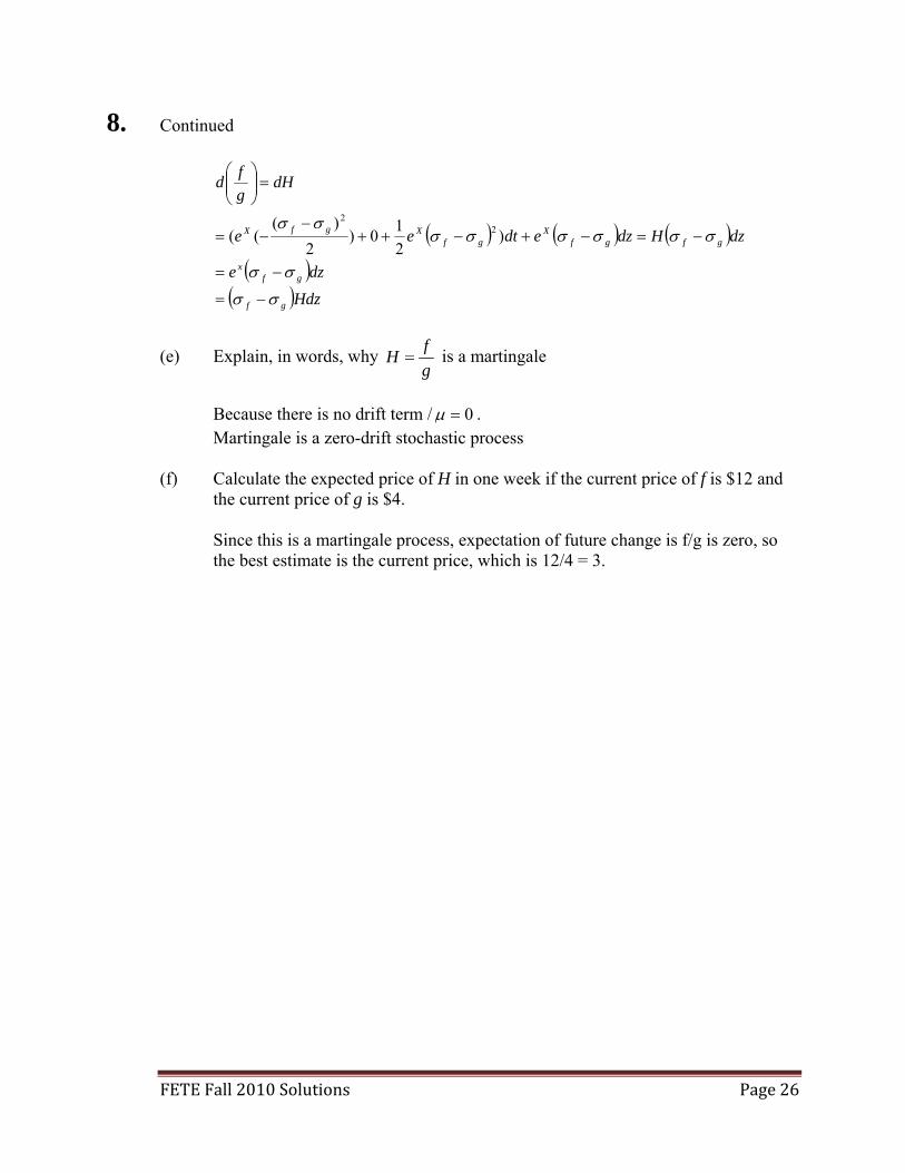
(e) Explain, in words, why f

Hg

is a martingale

Because there is no drift term / 0 . Martingale is a zero-drift stochastic process

(f) Calculate the expected price of H in one week if the current price of f is $12 and

the current price of g is $4. Since this is a martingale process, expectation of future change is f/g is zero, so the best estimate is the current price, which is 12/4 = 3.


9. Learning Objectives: 4. Financial Modeling Learning Outcomes: (4a) Describe and evaluate equity and interest rate models. Sources: Hull, J.C., Options Futures & Other Derivatives, 7th Edition, 2008 Ch. 28: Interest Rate Derivatives: The Standard Market Models Commentary on Question: This question asks candidates to demonstrate the application of Black’s model on caplet price to derive implied volatility. Part (a) required simple knowledge and understanding of how a caplet works. Part (b) required the candidates to use formulas provided to calculate the implied volatility. Overall, this was expected to be a fairly basic question. For part (a), this question was made overly complicated by many candidates trying to solve it from first principles; the 1 point value indicated that candidates should be done in about 3 minutes. Less than half of the candidates got the correct answer to this part. Because the price of a cap can be decomposed into the sum of caplet prices, the price of the caplet is simply the difference between the two observed cap prices. Some candidates incorrectly included additional discount factors or totaled all the observed prices. For part (b), the key to this question was identifying that the 2 normal distribution calls could be simplified into 1 call that can be back solved for. Most candidates understood how to set up the equation to solve for the vol. Those that got the formulas correct many times did not substitute the values correctly or make interpretations of the results. Many candidates struggled with the correct value of T[k+1] and the simplifying relationship between d1 and d2. Candidates generally did not do well on this part, thinking that it was impossible to solve and overlooked the identity with the normal distribution which allowed it to be solved analytically. Solution: (a) Calculate the time 1T caplet price.

Caplet = Price of Cap[1] – Price of Cap[.75] = 11.396 - 6.874 = 4.522

(b) Calculate the implied volatility for the 1T caplet for Black’s model.

Model Parameters are:

1

1 1.75 1 .25 0, 1 .03 10000 .03k k k k k kT T P T L F R


9. Continued

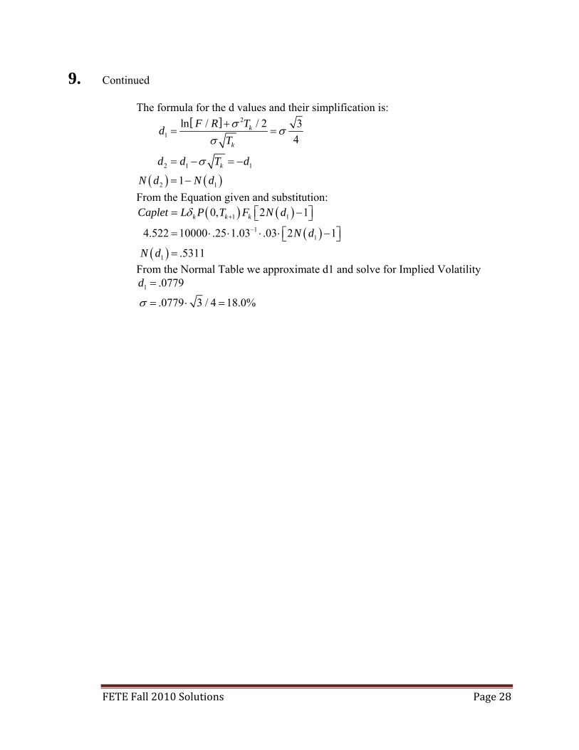
The formula for the d values and their simplification is:

2

1

2 1 1

2 1

ln / / 2 3

4

1

k

k

k

F R Td

T

d d T d

N d N d

From the Equation given and substitution:

1 1

11

1

0, 2 1

4.522 10000 .25 1.03 .03 2 1

.5311

k k kCaplet L P T F N d

N d

N d

From the Normal Table we approximate d1 and solve for Implied Volatility

1 .0779

.0779 3 / 4 18.0%

d


10. Learning Objectives: 1. Modern Corporate Financial Theory Learning Outcomes: (1d) Define and compare risk metrics used to quantify economic capital and describe

their limitations. (1e) Apply the concept of economic capital and describe methodologies for allocating

capital within a financial organization. Sources: Investment Guarantees, Hardy, 2003 Ch. 9: Risk Measures (pp. 157-169 only) Capital Allocation by Percentile Layer, by N. Bodoff Commentary on Question: The determination and allocation of different types of capital are important to risk management at an insurance company. The question tested candidates’ knowledge of the relationship between required surplus and free surplus as well as a correct application of the Bodoff algorithm. This question proved to be difficult, but a few candidates were, at a minimum, able to calculate required surplus, free surplus, losses which pierced the free surplus, and corresponding conditional exceedence probabilities of those losses. Many candidates expressed concern over the independence of the two distributions, claiming that it would have been too long a question. However, while this was a long question as asked it could be answered under the conditions presented. We remind the candidates to answer the question as asked and if they feel a question is too long to try to demonstrate understanding of the concepts being tested. The candidates should also know that it was not our intent to absorb huge amounts of time in arithmetic. There were four key concepts required for the successful completion of the question: Free surplus covers company losses in excess of the required capital level. Knowledge and understanding of how to calculate CTE. The problem asks only to allocate the free surplus using the capital allocation by

layers method; the Bodoff text example allocates all required surplus. The capital allocation by layers method requires determining the worst possible losses

that pierce the amount of capital in question and then working to the next worst, etc. This worst-down approach is clearly seen in the Bodoff text. Since the free surplus was the top layer of capital, we expected the candidates to begin to allocate starting with the greatest losses and working down similar to the text. We found that very few candidates used this approach and often times started from the bottom and incorrectly had only one event piercing that level of capital.


10. Continued

o Candidates who successfully answered the question tended to identify the above requirements to obtain a tractable problem setup: - The free surplus covers company losses at or just below $13 million. - Then the worst losses, beginning with $13 million loss (derived from UL $3

million + Term $10 million), were those that pierced free surplus and are used to determine the layers and subsequent allocations and conditional exceedence probabilities.

o Candidates who had difficulty with the allocation by layers calculations tended to

mischaracterize the relationship between free surplus and the risks/losses that pierced it. This most often led to layers of losses and conditional exceedence probabilities originating with the $0 UL and Term losses – using the smallest losses which did not pierce free surplus. Additionally assuming when the exceedence probabilities for the lowest level were calculated, they did not consider all the events that would pierce this level of capital.

o Overall, the candidates had difficulty with this question. Some of the this was

attributed to the question being very long as asked. However, we also believe there was a general lack of understanding of how to allocate by capital layers. Because of the overall scores on average being very low, this question ultimately had little effect on a candidates overall success or failure.

o The answer below is a complete answer to the question. In order to get full credit

on this question you would have only needed to write enough to demonstrate mastery of the four key concepts above.

Solution: Calculate the total amount of free capital for Carmenére Life and allocate the free capital to each of the two products by the allocation-by-layers method. Required Capital = 137.5% * CTE(97) A review of the loss distributions clearly shows that all combinations of the Term $10 million, $5 million, and $4 million losses are contained in the largest 3%, with a slight adjustment. Top 0.8% losses = Term $10 million + UL $x million Range from $13 million to $10 million Expected value = $10 million + E(UL losses) = $10.254 million Next 0.9% losses = Term $5 million + UL $x million Range from $8 million to $5 million Expected value = $5.254 million


10. Continued Next 1.3% losses = Term $4 million + UL $x million Range from $7 million to $4 million Expected value = $4.254 million Therefore the preliminary CTE(97) = [ 0.8%*10.254 + 0.9%*5.254 + 1.3%*4.254 ] / 3% = $6.154 million Of the Term $2 million losses, Term $2 million + UL $3 million = $5 million (4.5% * 0.8% = .036%) and Term $2 million + UL $2.6 million = $4.6 million (4.5% * 0.9% = .0405%) are actually in the top 3% replacing the same amount of the Term $4 million + UL $0 loss This adjustment is worth 0.036%*(5-4) + 0.405%*(4.6-4) / 3% = 0.000603/3% = 0.020 million Thus the CTE(97) = 6.154 + .0201 = 6.174 million And required surplus = 1.375 * 6.174 = 8.489 million And free surplus = 13 – 8.489 = 4.511 million The allocation-by-layers approach is to allocate this $4.511 million which means losses exceeding $8.489 million are those that pierce the free surplus. Event 1 = Maximum Possible Loss which penetrates into free surplus = $13 million = Term $10 million + UL $3 million Event 2 = Next largest loss = $12.6 million = Term $10 million + UL $2.6 million And similarly: Event 3 = $11.2 million = Term $10 million + UL $1.2 million, Event 4 = $11 million = Term $10 million + UL $1 million, Event 5 = $10.5 million Event 6 = 10.25 million Event 7 = 10 million Event 8 = 8 million = Term $5 million + UL $3 million does not pierce free surplus Thus, there are 7 layers.


10. Continued Layer 1 = $13 million - $12.6 million = $400,000 Layer 2 = $12.6 million - $11.2 million = $1,400,000 Layer 3 = $11.2 million - $11 million = $200,000 Layer 4 = $11 million - $10.5 million = $500,000 Layer 5 = $10.5 - $10.25 = $250,000 Layer 6 = $10.25 - $10. = $250,000 Layer 7 = $10 - $8.489 = $1,511,000 Probabilities: P(Event i) = P(Term loss contained in Event i) * P(UL loss contained in Event i) P(Event 1) = 0.008 * 0.008 = 0.000064 (Cumulative probability = 0.000064) P(Event 2) = 0.008 * 0.009 = 0.000072 (Cumulative probability = 0.000136) P(Event 3) = 0.008 * 0.013 = 0.000104 (Cumulative probability = 0.000240) P(Event 4) = 0.008 * 0.045 = 0.000360 (Cumulative = 0.0006) P(Event 5) = 0.008 * 0.101 = 0.000808 (Cumulative = 0.001408) P(Event 6) = 0.008 * 0.382 = 0.003056 (Cumulative = 0.004464) P(Event 7) = 0.008 * 0.442 = 0.003536 (Cumulative = 0.008) Only Event 1 penetrates Layer 1 and therefore receives 100% of surplus: Term(1) = Allocation to Term = $400,000 *

(share of Term in $13 million loss / Total loss of $13 million) = $400,000 * (10/13) = $308,000

Events 1 and 2 both penetrate Layer 2 and therefore share in the $1.4 million in relation to their share of the losses and the conditional exceedence probabilities: Term(2) = Allocation to Term = $1.4 million * (Term share of Layer 1) * (Conditional exceedence probability for Layer 1) + (Term share of Layer 2) * (Conditional exceedence probability for Layer 2) = $1,400,000 * [(10/13)*(0.000064/0.000136) + (10/12.6)*(0.000072/0.000136)] = $1,095,000 Similarly, Term(3) = Allocation to Term = $200,000 * (Term share of Layer 1) * (Conditional exceedence probability for Layer 1) + (Term share of Layer 2) * (Conditional exceedence probability for Layer 2) + (Term share of Layer 3) * (Conditional exceedence probability for Layer 3) = $200,000

* [(10/13)*(0.000064/0.00024) + (10/12.6)*(0.000072/0.00024) + (10/11.2)*(0.000136/0.00024)]

= $166,000


10. Continued Term(4) = $500,000

* [(10/13)*(0.000064/0.0006) + (10/12.6)*(0.000072/0.0006) + (10/11.2)*(0.000136/0.0006) + (10/11)*(0.00024/0.0006)]

= $439,000 Term(5) = $250,000

* [(10/13)*(0.000064/0.001408) + (10/12.6)*(0.000072/0.001408) + (10/11.2)*(0.000136/0.001408) + (10/11)*(0.00024/0.001408) + (10/10.5)*(0.0006/0.001408)]

= $230,000 Term(6) = $250,000

* [(10/13)*(0.000064/0.004464) + (10/12.6)*(0.000072/0.004464) + (10/11.2)*(0.000136/0.004464) + (10/11)*(0.00024/0.004464) + (10/10.5)*(0.0006/0.004464) + (10/10.25)*(0.0006/0.004464)]

= $240,000 Term(7) = $1,511,000

* [(10/13)*(0.000064/0.008) + (10/12.6)*(0.000072/0.008) + (10/11.2)*(0.000136/0.008) + (10/11)*(0.00024/0.008) + (10/10.5)*(0.0006/0.008) + (10/10.25)*(0.0006/0.008) + (10/10)*(0.0006/0.008)]

= $1,476,000 Term allocation = Sum Term(1) through Term(7) = 3.954 million UL allocation = 4.511 million – 3.954 million = 0.557 million


11. Learning Objectives: 2. Corporate Financial Applications Learning Outcomes: (2b) Describe the process, methods and uses of financial reinsurance (surplus relief)

and recommend a structure that is appropriate for a given set of circumstances. (2c) Describe the process, methods and uses of insurance securitizations and

recommend a structure that is appropriate for a given set of circumstances. Sources: FET-148-08: Securitization of Life Insurance Assets and Liabilities Pg. 3-13, 40-42 FET-161-08: Tiller & Tiller, Life, health and Annuity Reinsurance, Ch. 5: Advanced Methods of Reinsurance Pg. 142-143 Commentary on Question: This is a recall, application and analysis integrated question asking candidates to utilize the concept of financial reinsurance and securitization to deal with surplus strain problems. In general, part (b) of this question was answered well. Many candidates could demonstrate their understanding of financial reinsurance and securitization structure. However, very few candidates answered part (c)(iii) and part (d) correctly. Part (c) iii) is a very simple application of option theory. Most candidates did not realize part (d) is related to part (a) to (c) and just repeated part (b). Solution: (a) Determine the reduction in first year surplus strain in Solution 1.

Before reinsurance after tax surplus strain = - (Gross Premium + Inv. Inc - Commission - Expenses - Death Benefits - Change in Reserves) * (1-tax rate) = - (4000+80-2400-1200-320-2400)* (1-30%) = 1568 After reinsurance Net premium (NP) = 4000 * (1-30%) = 2800 Net Investment Income (NI) = 80 ModCo adjustments (MA) = 2400 * 30% = 720 Commissions (C) = 2400 * (1 - 30%) = 1680 Allowance (A) = 15% * 4000 * 30% = 180


11. Continued

Expense (E) = 1200 * (1 - 30%) = 840 Death Benefit (DB) = 320 * (1 – 30%) = 224 Change in Reserves (R) = 2400 Surplus strain after tax = - (NP + NI + MA + A - C - E - DB – R) * (1 – tax rate (30%)) = 955 Reduction in after tax surplus strain = 1568 - 955 = 613

(b) Briefly describe the economic rationale for securitization.

Creation of new classes of securities Facilitate risk management Add liquidity to financial market Improve market efficiency and capital utilization Unlock embedded profits in a block of business Reduce cost of capital Increase ROE, improve other operating measures

(c) Specific to Carmenére Life’s Solution 2,

(i) Explain how the securitization of the Term Life in-force block would address Carmenére Life’s Universal Life surplus strain problem.

Securitization takes the Term Life cash flows promised to Carmenére Life in the future and sells them for $ 7 million Securitization costs of 6.7 million gives net of 0.3 million used to reduce surplus strain

(ii) Describe the cash flows (I, II, III, IV) and role each party plays.

(I) - Carmenére Life makes payments equal to the expected mortality costs under the Term Life block to Rosé Capital (SPV)

(II) - Carmenére Life will receive payments from Rosé Capital based on actual mortality experiences under the block.


11. Continued

(III) - Rosé Capital would issue mortality notes to investors

(IV) - Investors pay proceeds to Rose Capital for mortality notes

(iii) Derive a function for the option payoff in terms of CM (Cumulative Mortality) and D (Actual deaths in the indexed pool of 2010).

Option payoff lower strike piece = MAX (CM - 125% D, 0)

Option payoff upper strike piece = MAX (CM - 150% D, 0)

Option payoff = (MAX (CM -125%D, 0) – MAX (CM -150% D, 0) / 25%D

(d) Outline 2 or 3 advantages for both solutions and recommend a solution for

Carmenére Life.

Mortality securities uncorrelated with financial markets.

Rating agencies tend to view securitization favorably. Cost of reinsurance is better for insignificant deals. Reinsurance takes less time to implement.

Net decrease in surplus strain is bigger for the reinsurance (613K vs. 300 K) for securitization.

The reinsurance option can be done in a shorter period of time.

Hence, Solution 1 is the recommendation.


12. Learning Objectives: 1. Modern Corporate Financial Theory Learning Outcomes: (1f) Identify regulatory capital requirements and describe how they affect decisions. Sources: “A Comparative Analysis of US, Canadian, and Solvency II Capital Adequacy Requirements in Life Insurance,” Sharara, Hardy and Saunders. Commentary on Question: This question tested the new syllabus material by Shahara, Hardy and Saunders. The question asked for only the components regarding investment risk. Additionally, we did not want the candidates doing a brain dump of everything out of that study note, hence we reduced the scope of the question and only gave credit for that which addressed the question.

A sizable number of candidates misinterpreted the valuation of investment risk to apply to the valuation of the liabilities.

Most candidates answered part (b)(i) well. Most candidates did not answer part (b)(ii) in the manner expected, giving implications of Solvency II rather than actions companies would take to manage the risks. Solution: (a) Describe how investment risk is assessed by the capital adequacy requirements of

the Canadian and U.S. regulatory capital regimes. Address: (i) Valuation methodologies

Canada: Assets held for trading (HFT) or Available for Sale (AFS) AFS held to maturity Realized capital gains/losses not in available capital Unrealized Gains/losses included in available capital US: Assets held at market value, amortized cost, equity method, Book Value (cost) IMR = Moderates impact from interest related gains AVR = Smooths impact from credit defaults and equity risk related gains/losses


12. Continued

(ii) Capital formulas

Canada: C1 Risk – Risk of loss resulting from on-balance sheet asset default and contingencies in respect of off-balance sheet exposure and related loss of income; and the loss of market value of equities and related reduction of income Factor based approach

US: C0 - Asset Risk Affiliates C1cs – Unaffiliated Common Stock C10 – Asset Risk Other C3a – Interest Rate Risk and Market Risk Factor based approach

(iii) Diversification benefits

Canada: No diversification benefits US: Diversification of Asset Risk other with Interest Risk and Market Risk

(b)

(i) Compare Solvency II investment risk regulatory requirements in Canada and the U.S.

Valuation: Assets marked to market or marked to model if unavailable Assets valued on an economic basis. Capital requirement: Assess market risks including: Interest rate risk, equity, credit spread, forex, property risk SCR = solvency capital requirement = net impact of TSBR due to assumption change from best estimate to capital requirement Total SCR = SQRT[sum over i,j (correlation i,j) * SCR i * SCRj] Company can employ internal model to get reduced capital for Capital market hedging programs. Significant diversification benefit under Solvency II


12. Continued

(ii) Describe the impact of Solvency II on Canadian and U.S. insurer decisions on portfolio allocation.

Interest rate risk less for US and Canada since having fixed factors tied to liabilities No reinvestment in Canadian model Canadian framework has incentive to invest in riskier assets and arbitrage the regulatory environment US framework is risk insensitive since liabilities are valued at fixed rate Solvency II delinks liability and asset valuation


13. Learning Objectives: 1. Modern Corporate Financial Theory Learning Outcomes: (1d) Define and compare risk metrics used to quantify economic capital and describe

their limitations. Sources: Investment Guarantees, Hardy, 2003, Ch. 8: Dynamic hedging for separate account guarantees Ch. 9: Risk Measures (pp. 157-169 only) Commentary on Question: This question was pulled directly out of the Hardy text (Chapter 9) but the numbers were changed to make the option go into the money more often than normal. Only formulas on formula sheet were needed to solve parts (a) and (b). The range was provided for part (b) so that in the event part (b) was too difficult or done incorrectly, the answer could be used to give some commentary to part (c). Overall candidates did fairly well on this question. Generally for parts (a) and (b) the candidates either did it completely correct or completely incorrect with a handful that got partial credit. Some candidates even got the correct answer without using the formulas on the formula sheet directly but instead derived the formula. The candidates who did the question wrong usually did not understand the variables in the formula. For part (c) only a handful of candidates got significant points. Solution: (a) Calculate the probability that the GMMB matures in the money.

ξ = 1 - Φ [ (log G/S0 – n(μ + log (1 – m))) / (√n σ) ] Formula 9.4 Question asked for probability of GMMB maturing in the money so need to use 1 - ξ G/S0 = .8 n=120 μ = .005 m=.0015 σ = .06 = Φ [ (ln(.8) – 120 (0.005 + log (1 – 0.0015))) / (√120 * 0.06) ] = Φ(-0.978) = 0.164


13. Continued (b) Calculate the 95% Value at Risk (VaR) for the present value of the GMMB

liability at inception, showing that it falls within the range $42 to $48.

VaR95% = (G – F0 exp(- za*√n* σ + n(μ + log (1 – m))e^(-rn) (formula 9.7) G = 200 F0 =250 za = 1.644 n=120 σ = .06 μ = .005 m=.0015 e^(-rn) = e(-.05*120/12) = .6065 VaR95% = (200 – 250 exp(-1.644*√120 * .06 + 120(.005 + log (1 – .0015))*.6065 = 43.03

(c) Outline the points you would make in response to this comment.

1. The CEO is right about PV MC, = 41.2 (eqn 8.14 in Hardy).

2. But risk is non-diversifiable, so number of policies is not very relevant. Lots of small policies maturing at the same time represent same risk as one big one.

3. The CTE shows significant additional risk if the 5% worst case transpires - $15 over the expected MC;

4. And if the MC isn’t hedged, it will be worse, because the MC income falls when the guarantee moves into the money.

5. Option price also demonstrates that this is not a free option.

6. Better to hedge the option at, approximately, the option price, to mitigate risk and minimize economic capital requirement.


14. Learning Objectives: 2. Corporate Financial Applications Learning Outcomes: (2d) Evaluate alternate options for utilizing capital and recommend the most

appropriate use in a given situation. Sources: Copeland, Weston, Shastri, Financial Theory and Corporate Policy, 4th Edition, Ch. 15: Capital Structure and the Cost of Capital: Theory and Evidence Commentary on Question: This question was designed to examine WACC in a more advanced context. Part (a) was a pretty straight forward calculation for most candidates. Part (b) relied on knowledge of equation (15.67) for parts (i) and (ii) VL(V) = VU(V) + Tc*B(V) – DC(V) = VU(V) + Tc*B + Tc*B – pB*Tc*B – aVB*pB and equation (15.19) in part (iii) WACC = p * (1-t*B/(B+S)). For part (b)(iii), many candidates used the WACC formula (1-t)*Kb*B/(B+S) + Ks*S/(B+S). This formula is acceptable and correct. However, it requires the candidate to recalculate Ks and Kb for each debt level, which many failed to do correctly. Solution: (a) Determine the value of Petit Verdot Inc.

Equation (15.2) from the text cost of equity for an all-equity firm (p) = rf + beta * market risk premium p = 4% + 2 * 3% = 10% Long term value of firm = S = EBIT * (1 - tax rate) / p S = (1 - 35%) * 10 million / 10% = 65 million

(b) Calculate under the four different debt scenarios:

(i) Expected value of the tax benefit from the deductibility of interest payments

Tax benefit from deductibility of interest = debt value * tax rate * (1 - PV of $1 contingent on future business disruption), or in mathematical equation form Tc*B(V)= Tc*B – pB*Tc*B = Tc*B * (1-pB). 6.5 million debt level: 6.5 million * 35% * (1 - 0.2) = 1.820,000 8.5 million debt level: 8.5 million * 35% * (1 - 0.25) = 2,231,250 10.5 million debt level: 10.5 million * 35% * (1 - 0.30) = 2,572,500 12.5 million debt level: 12.5 million * 35% * (1 - 0.35) = 2,843,750


14. Continued

Note: The following alternative solution was used by several candidates and was acceptable for full marks, which is the Tc*B part of the expected solution. This is the definition of tax benefit from equation (15.6) instead of (15.67). Tax benefit from deductibility of interest = debt value * tax rate, or in mathematical equation form Tc*B(V)= Tc*B. 6.5 million debt level: 6.5 million * 35% = 2.275 million 8.5 million debt level: 8.5 million * 35% = 2.975 million 10.5 million debt level: 10.5 million * 35% = 3.675 million 12.5 million debt level: 12.5 million * 35% = 4.375 million Although the alternative is acceptable for part (b)(i), the expected solution is required in part (c) for full marks. A candidate that submits the alternative for (b)(i) would need to recalculate the remaining parts of expected solution, namely multiplying the alternative solution by (1-pB), to get full marks in part (c) below. A common error in this part was multiplying the cost of debt by the debt value.

(ii) Expected present value of the business disruption costs

Use aVB*pB from equation (15.67) Present value of disruption cost = PV of $1 * disruption cost = aVB*pB 6.5 million debt level: 275,000 * 0.2 = 55,000 8.5 million debt level: 300,000 * 0.25 = 75,000 10.5 million debt level: 325,000 * 0.30 = 97,500 12.5 million debt level: 400,000 * 0.35 = 140,000

(iii) Petit Verdot’s weighted average cost of capital.

Use weighted average cost of capital = p * (1 - tax rate * D / (D + S)) 6.5 million debt level: 10% * (1 - 35% * 6.5/ (65 + 6.5)) = 9.68% 8.5 million debt level: 10% * (1 - 35% * 8.5/ (65 + 8.5)) = 9.60% 10.5 million debt level: 10% * (1 - 35% * 10.5 / (65 + 10.5)) = 9.51% 12.5 million debt level: 10% * (1 - 35% * 12.5 / (65 + 12.5)) = 9.44%


14. Continued

(c) Evaluate the benefits of the four debt scenarios in terms of optimal capital structure and recommend the best alternative for Petit Verdot.

The Net Benefit is the increase in value, or a portion of equation (15.67) Tc*B – pB*Tc*B – aVB*pB Net benefit = tax benefit - PV disruption cost = Tc*B – pB*Tc*B – aVB*pB = Tc*B(V) – DC(V) Highest net benefit = optimal capital structure 6.5 million debt level: 1,820,000 - 55,000 = 1,765,000 8.5 million debt level: 2,231,250 - 75,000 = 2,156,250 10.5 million debt level: 2,572,500 - 97,500 = 2,475,000 12.5 million debt level: 2,843,750 - 140,000 = 2,703,750 Debt level 12.5 million has the highest net benefit Therefore, 12.5 million debt level has the optimal capital structure


15. Learning Objectives: 5. Efficient Markets & Information Theory Learning Outcomes: (5e) Define the elements of a game, including information sets, etc., Nash equilibrium,

mixed strategies; explain the prisoners' dilemma and other special cases of a two-person, two-state, single period game, and explain the qualitative implications of repeated games.

Sources: FET-156-08: “An Introduction to Applicable Game Theory,” by Gibbons, R., Journal of Economic Perspectives, Winter 1997, pp. 127-149. Commentary on Question: The question draws on material presented in Study Note FET-156-08 by Robert Gibbons. In that Note, Gibbons presents a number of game tree illustrations for his example problems. On page 134, he includes both a paragraph describing the payoffs in the problem and a game tree diagram. The game tree diagram includes payoffs at the end of each branch and uses the convention that the upper position payoff applies to the player first to act while the lower position payoff applies to the second player. He continues to use this convention on page 143 in a game tree diagram that is similar to the one used in this question. This question assumes familiarity with the example on page 143 of the study note. A candidate familiar with that example is expected to be able to create the normal form payoff table associated with that diagram. The candidates overall did very well on this question. Solution: (a) Show the normal form representation of this game. Player CB A' B'

A 20,10 0,0(GNI, CB)

Player GNI

B 0, 20 0, 10

R 10,30

10, 30


15. Continued (b) Define a Nash Equilibrium.

A Nash Equilibrium is a combination of strategies where each player's strategy is the best response to the other player's strategy.

(c) Identify all pure-strategy Nash Equilibria for this game.

(A, A') and (R, B') are Nash equilibria. (d) Calculate CB’s expected payoff for A and B .

E[A'] = p ( 10) + (1 - p) 20 = 20 -10p

E[B'] = p( 0 ) + (1-p) 10 = 10- 10p

(e) Determine the impact on CB’s strategy.

The expected payoff of A' is always higher than the expected payoff of B'; therefore CB will always choose A'.

(f) Determine the impact, if any, to the Nash Equilibria.

(A, A') is still a Nash Equilibrium.


16. Learning Objectives: 3. Derivatives and Pricing Learning Outcomes: (3f) Demonstrate mastery of option pricing techniques and theory for equity and

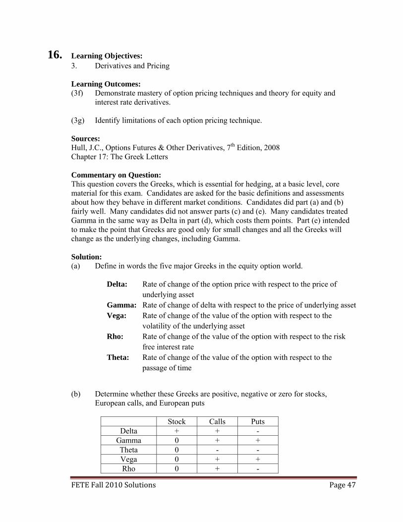
interest rate derivatives. (3g) Identify limitations of each option pricing technique. Sources: Hull, J.C., Options Futures & Other Derivatives, 7th Edition, 2008 Chapter 17: The Greek Letters Commentary on Question: This question covers the Greeks, which is essential for hedging, at a basic level, core material for this exam. Candidates are asked for the basic definitions and assessments about how they behave in different market conditions. Candidates did part (a) and (b) fairly well. Many candidates did not answer parts (c) and (e). Many candidates treated Gamma in the same way as Delta in part (d), which costs them points. Part (e) intended to make the point that Greeks are good only for small changes and all the Greeks will change as the underlying changes, including Gamma. Solution: (a) Define in words the five major Greeks in the equity option world.

Delta: Rate of change of the option price with respect to the price of underlying asset

Gamma: Rate of change of delta with respect to the price of underlying asset Vega: Rate of change of the value of the option with respect to the

volatility of the underlying asset Rho: Rate of change of the value of the option with respect to the risk

free interest rate Theta: Rate of change of the value of the option with respect to the

passage of time

(b) Determine whether these Greeks are positive, negative or zero for stocks,

European calls, and European puts

Stock Calls Puts Delta + + -

Gamma 0 + + Theta 0 - - Vega 0 + + Rho 0 + -


16. Continued (c) For each of the above scenarios, determine whether a positive or negative delta,

gamma, or vega in your trading book would produce a profit. Positions Scenario Market Conditions Delta Gamma Vega

1 Swift Downward Price

Movement; Rising Implied Volatility

- Increases Gain

+ Increases Gain

+ Increases Gain

2 No Price Movement;

Falling Implied Volatility Does Not

Matter Does Not

Matter - Increases

Gain

(d) Estimate the value change in your trading book at closing today.

Option Units Delta Gamma Theta/Day Vega Stock Price Movement

Change In Volatility

Call Totals -600 -736 -14.8 +0.5 -0.8 -4 +2 Put Totals 400 -618 -2.6 +0.2 -0.1

Stock 1200 1200 0 0 0 Total 1000 -154 - 17.4 +0.7 -0.9

New delta = delta + gamma * price change

= -154-17.4 * (-4) = -84.4

Average delta = (-154 -84.4)/2 = -119.2

Change of value = -119.2 *(-4) + 0.7 -0.9 * 2

= 475.7 (e) Explain how the value of your trading book will change if Tempranillo Corp.

stock falls 50%.

The stock holding will lose 50%. The Puts will gain at a rate approaching 50%; the short calls will have essentially no price change as they’re so far OTM. As the put $delta is less than the stock the book is underhedged, so the position will lose money. Or The total delta position is negative indicates that the book makes money for a small movement in the stock price. Delta and other Greeks will change as the stock moves. The book is net long in notional (1200-400-600) = 200, so the book will lose money for a big drop in the stock price.


17. Learning Objectives: 4. Financial Modeling Learning Outcomes: (4a) Describe and evaluate equity and interest rate models. (4e) Recommend an equity or interest rate model for a given situation. (4g) Describe how option pricing models can be modified or alternative techniques

that can be used to deal with option pricing techniques’ limitations. Sources: Hull, J.C., Options Futures & Other Derivatives, 7th Edition, 2008 Ch. 21: Estimating Volatilities and Correlations “Validation of Long-Term Equity Return Models for Equity-Linked Guarantees” by Hardy, Freeland and Till, NAAJ Vol. 10 No. 4, October 2006 (Sections 1-4 only) Commentary on Question: This question is testing candidates’ knowledge on the modeling of volatility with common stochastic investment models. In general, candidates performed well in the calculations involved in this question. However, many had difficulty with the translation of the mathematical equations to intuitive explanations. For part (a), there are three common mistakes found in this question: Some candidates answered using formulas whereas the question specifically asked for

words. Some candidates read the question as, “What are the characteristics of each of the

models.” Some candidates answered by re-wording the question. For example, “The RSLN-2

model is a lognormal model that switches between two regimes.” Part (b) proved to be a very difficult question for most candidates. Many candidates were confused as to whether p-value was “good” or “bad”. Most candidates failed to adjust the max log-likelihood values for the number of parameters. Part (c)(i) is where the candidates earned the most points. For part (c)(ii), some candidates took positions “for” and “against” the colleague but failed to take a final stand.


17. Continued Solution: (a) Describe the volatility process in words for each of these models, explaining how

the process is stochastic.

The GARCH model is deterministic projecting the first period ahead and stochastic for projecting periods after the first. The GARCH variance is a weighted average of long term variance, the previous period variance and an innovation term from the previous time period. The volatility in this model can increase suddenly, but it will tend back to the long run value (mean reversion), similar to the way guitar strings twang and then stabilize. This model is a stochastic process because of its dependence on the previous time period. The RSLN-2 model has 2 volatilities, one for each of its 2 states. The volatility process is stochastic as it moves between the two states following a Markov process. The Markov process depends on the current state rather than a historical state. The RDDD-2 model is identical to the RSLN-2 model except there is an additional drawdown term which adds pressure to the volatility to return to the previous high-water mark whenever the volatility drops below that high-water mark.

(b) Determine which model provides the best overall fit to the equity index in

question, based on this information. Justify your selection.

GARCH: According to the J-B test, the residuals are not normal so the model does not fit the data. RSLN and RSDD both have p-values that pass the J-B test. The number of parameters need to be considered. The RSDD has 8, the RSLN has 6 so the RSDD is penalized more than RSLN. Consider 2 tests: AIC and BIC BIC: Choose the higher value of

(max log-likelihood) – (.5) x (# of parameters) x ln(# values) RSLN: 663.2 – (.5) (6) ln(379) = 645.4 RSDD: 664.3 – (.5) (8) ln(379) = 640.6

Therefore, RSLN should be chosen.


17. Continued (c)

(i) Calculate the long run volatility for this GARCH model expressed as an annual rate.

Formula for long run volatility (= ): 2 = 0 / (1 – 1 – ) = square root of [.006922 / (1 - .121 - .869) ] = 6.92% To annualize this monthly value, multiply by square root of 12 = 23.97%

(ii) Outline the points you would make in reply. You should state whether or

not you agree with your colleague. You should assume her calculation is correct.

Volatility is important but it’s often not a good measure of risk. GARCH volatility tends to be symmetric which understates the risk of

lower returns in the left tail. Also, if the volatility is symmetric, too much emphasis is given to the ‘up scenarios’ where risk is non-existent for the GMMB.

The high Beta in the GARCH model means the model has a slow mean reversion to the long term volatility.

The high volatility regime within RSLN is partnered with a lower mean so there’s a higher probability of low returns which is more conservative for a GMMB.

If there are longer periods in the high volatility regime (RSLN) there could be more weight in the left tail which is important for a GMMB.

The importance of which model to use is affected by whether or not there are any hedging practices in place. The long term volatility may not be as important as the day-to-day or month-to-month modeling.

Based on these points, I would disagree with my colleague.


18. Learning Objectives: 4. Financial Modeling Learning Outcomes: (4a) Describe and evaluate equity and interest rate models. Sources: Hull, J.C., Options Futures & Other Derivatives, 7th Edition, 2008 Ch. 19: Basic Numerical Procedures, Ch. 28: Interest Rate Derivatives: The Standard Market Models FET-159-08: Babbel, D. & Fabozzi, F.J., Investment Management for Insurers, 3rd Edition, Ch 13: “Problems Encountered in Valuing Interest Rate Derivatives” by Y. Pierides “Validation of Long-Term Equity Return Models for Equity-Linked Guarantees” by Hardy, Freeland and Till, NAAJ Vol. 10 No. 4, October 2006 (Sections 1-4 only) Commentary on Question: This question is about valuing an interest rate derivative by Monte Carlo simulation and discussing the appropriateness of the simulation result for listed applications. For part (a), many candidates forgot to multiply by 0.25 to get the quarterly payment. Another common mistake was to calculate the payoff of a swap rather than a cap. Others tried to calculate the value of the option, for which there is no information. For part (b) in (i), some candidates incorrectly cited calculating the average of payoffs before taking the present value. In (iii) some candidates incorrectly cited applying the shock to the scenario rates directly. In (iv), most candidates correctly stated the definition of the CTE98 but failed to justify their answer on appropriateness of calculation. Solution: (a) Calculate the payoff of the 1-year interest rate cap with a $500 million notional

using the outcome from this scenario. Lδk MAX( Rk – RK, 0) for payoff at time tk+1 (formula 28.5 of Hull’s) RK = 3% The payoff at time 0, 0.25 and 0.5 is all zero since Rk <= 3% At t=0.75, the payoff is 500M x 0.25 x max(3.1349%-3%,0)=168,628 At t=1.00, the payoff is 500M x 0.25 x max(3.047%-3%,0)=58,750


18. Continued (b) Evaluate the appropriateness of using these simulations for each of applications

(i) through (iv), and, when appropriate, describe how to proceed.

(i) Estimate the price of the cap. Appropriate, because of q-measure. The price is equal to the discounted expectation of its payoffs.

(ii) Determine the error of the estimated price.

Appropriate, because the standard error of the estimate is M

, where M is the number of trials and ω is the standard deviation.

(iii) Calculate the sensitivity of the price to movement in the short rate Not appropriate, because the rate is constant in all scenarios. Need to generate another 1000 scenarios with a small change in the rate.

(iv) Calculate CTE(98) Not appropriate, as LMM is a q-measure model for pricing, and CTE is a p-measure risk measure. CTE(98) = take the average of worst 20, which 2% of worst outcome.

Documents

FETE Complete Illustrative Solutions Fall 2010 1. · FETE Complete Illustrative Solutions Fall 2010 1. ... the weighted average cost of capital is: WACC = (1-rc) ... FETE Fall 2010