Fertility and Wars: The Case of World War I in Franceguillaumevdb.net/ww1_Final.pdf · Fertility and Wars: The Case of World War I in France ... Jones, Schoonbroodt, ... There were

108

American Economic Journal: Macroeconomics 2014, 6(2): 108–136 http://dx.doi.org/10.1257/mac.6.2.108

Fertility and Wars: The Case of World War I in France†

By Guillaume Vandenbroucke*

During World War I, the birth rate in France fell by 50 percent. Why? I build a model of fertility choices where the war implies a positive probability that a wife remains alone, a partially-compensated loss of a husband’s income, and a temporary decline in productivity followed by faster growth. I calibrate the model’s key parameters using pre-war data. I find that it accounts for 91 percent of the decline of the birth rate. The main determinant of this result is the loss of expected income associated with the risk that a wife remains alone. (JEL D74, J13, J24, N33, N34, N44)

During the First World War (1914–1918) the birth rate in France declined by about 50 percent.1 The resulting deficit in births is estimated to be 1.4 million,

which is equal to the estimated loss of French lives due to the war.2 It follows that the decline of the birth rate doubled the already large demographic impact of the war, and its effect on the French demography was noticeable well into the twentieth century. I offer a theory to account for this phenomenon.

I develop a model that builds upon Greenwood, Seshadri, and Vandenbroucke (2005). The unit of analysis is a finitely-lived household made of adults and chil-dren. The household derives utility from consumption as well as from the number of children it chooses to have. However, children are costly. They require that the wife devotes a fixed fraction of her productive time to them as long as they remain in the household. In this model, the war matters because the (likely) death of a husband is a pure, negative (expected) income shock. Since children are normal goods, the war negatively affects births.

I propose a quantitative exercise consisting of two steps. First, I calibrate the model to fit the time series of the French birth rate from 1800 until the eve of World War I. Second, I use the calibrated model to evaluate the effects of the war on births. I model the war as a change in the environment facing a household along three

1 See Figure 1.2 See Figure 2 for the size of the birth deficit. See Huber (1931, 431) for military losses. Military losses include

people killed and missing in action. They do not include civilian losses.

* University of Southern California, Department of Economics, KAP 300, Los Angeles, CA, 90089 (e-mail: [email protected]). This paper was initially circulated under the title “Optimal Fertility During World War I.” I thank three anonymous referees helpful comments. I am grateful to Patrick Festy for pointing out relevant data sources and sharing some of his own data. I also thank John Knowles, Juan Carrillo, Cezar Santos, Oksana Leukhina, David Lagakos, Alice Schoonbroodt, and seminar participants at University of Southern Carlifornia Marshall School of Business, University of New South Wales, the 2012 Midwest Macro Meetings, the 2012 National Bureau of Economic Research (NBER) conference on Macroeconomics across Time and Space, the 2012 CMSG meetings, and University of California-Riverside for useful comments.

† Go to http://dx.doi.org/10.1257/mac.6.2.108 to visit the article page for additional materials and author disclosure statement(s) or to comment in the online discussion forum.

http://dx.doi.org/10.1257/mac.6.2.108

mailto:[email protected]


VoL. 6 No. 2 109Vandenbroucke: fertility and wars: the case of wwi in france

dimensions: (i) a positive probability that a wife remains alone; (ii) a partially compensated loss of a husband’s income; (iii) a temporary decline in productivity, followed by faster growth.

The calibrated model accounts for 91 percent of the observed decline of the birth rate during the war. The key determinant of this result is the loss of expected income associated with the risk that a wife remains alone, that is (i). Other forces, that is (ii) and (iii), are quantitatively relevant taken one by one, but together they almost offset each other since a drop in earnings for a wife reduces the opportunity cost of raising children, while for the husband it implies a negative income effect. The model also predicts an increase in the birth rate (4 percent more than in the data) after the war, fueled by a catch-up effect.

This paper contributes to a literature analyzing the consequences of WWI on various aspect of the French population.3 Henry (1966) documents the consequences of the war on the marriage market. More recently, Abramitzky, Delavande, and Vasconcelos (2011) evaluate the impact of the war on assortative matching in the marriage market, and Knowles and Vandenbroucke (2013) propose a model of the postwar behavior of marriage and fertility rates. The closest studies are by Festy (1984) and Caldwell (2004). Festy (1984) offers a detailed description of the decline of births during the war. He concludes that “the decline of births during hostilities can be seen as a ‘mechanical’ consequence of the impossibility of procreating, rather than a deliber-ate attempt to avoid giving birth in such a troubled period.” 4 In short, Festy’s theory is that feasible births declined while desired births remained constant. In this paper, I propose a different approach: even without a reduction in feasible births, how far can a reduction in desired births go in accounting for the actual decline? Caldwell (2004) examines 13 social crises, ranging from the English Civil War in the seventeenth cen-tury to the fall of communism. He documents noticeable drops in birth rates in each case, and concludes that they were mostly temporary adjustments to the uncertainty of the time. His results are consistent with the analysis that I carry out in this paper.

There are other economic theories of fertility beside the one on which I build my model. Many are reviewed in Jones, Schoonbroodt, and Tertilt (2011). A well-known alternative is the so-called “quality-quantity” tradeoff theory proposed by Becker (1960). In these models, increases in wages induce parents to substitute the quantity of children for higher quality. It is worth noting that, if there is still a time cost of raising children paid by the wife only, then the effect of the war on fertility is, qualitatively, the same as in the model presented here. Thus, the analysis in this paper will carry over to alternative setups.

3 This paper is also related to an already large literature focusing on the determinants of fertility across countries and over time. Seminal work was done by Becker and Barro (1988) and Barro and Becker (1989). Other authors have explored various aspects of fertility choices. Galor and Weil (2000) analyze the ∩-shaped pattern of fertility over the long run. Greenwood, Seshadri, and Vandenbroucke (2005) and Doepke, Hazan, and Maoz (2007) propose theories of the baby boom in the United States. Jones, Schoonbroodt, and Tertilt (2011) review alternative theories explaining the negative relationship between income and fertility across countries and over time. Albanesi and Olivetti (2010) evaluate the effects of technological improvements in maternal health. Jones and Schoonbroodt (2011) theorize endogenous fertility cycles. Manuelli and Seshadri (2009) ask why do fertility rates vary so much across countries?

4 The quote from Festy is: “La chute de la natalité pendant les hostilités peut donc être vue, par différence, comme une conséquence ‘mécanique’ de l’impossibilité de s’unir pour procréer, plutôt que comme une volonté délibérée d’éviter d’avoir des enfants dans une période aussi troublée.” (Festy 1984, 1003).

110 AMErIcAN EcoNoMIc JourNAL: MAcroEcoNoMIcs AprIL 2014

In the next Section, I present statistics relative to the number of births and deaths during the war as well as to the composition of the army. I also discuss relevant facts pertaining to the marriage market and the situation of women during the war. I develop my model and discuss the determinants of optimal fertility in Section II. I present the quantitative analysis and the results in Section III. I conclude in Section IV.

I. Facts

Some data are from the French census. The last census before the war was in 1911. The first census in the postwar era was in 1921. A census was scheduled in 1916 but was cancelled. This data, and the data from previous censuses, were sys-tematically organized in the 1980s and made available from the Inter-University Consortium for Political and Social Research (ICPSR). It is also available from the French National Institute for Statistics and Economic Studies (Insee). Vital statistics are available during the war years for the 77 regions (départements) not occupied by the Germans. There were a total of 87 regions in France at the beginning of the war. Huber (1931) provides a wealth of data on the French population before, during, and after the war. It also contains a useful set of income-related data.

A. Births and Deaths

The first month of WWI was August 1914, but the first reduction in the number of live births occurred nine months later. It dropped from 46,450 in April 1915 to 29,042 in May—a 37 percent decline.5 During the course of the war the minimum was attained in November 1915 when 21,047 live births were registered. The prewar level of births was reached again in December 1919. To put these numbers in per-spective consider Figure 2, which shows the number of births per month in France and Germany. For France, the difference between the actual number of births and the trend, summed between May 1915 (nine months after the declaration of war) and August 1919 (nine months after the armistice), yields an estimated 1.4 million children not born. This figure amounts to 3.5 percent of the French population in 1914 (40 million) and is comparable to the military losses of the war, 1.4 million. The estimate for Germany is 3.2 million children not born. It amounts to 5 percent of the German population in 1911 (65 million) and exceeds the number of military deaths estimated at 2 million.6 Similar calculations, made by demographers, lead to comparable figures. Vincent (1946, 431) reports a deficit of 1.6 million French births and Festy (1984, 979) reports 1.4 million.7

Figure 1 and Figure 2 show changes in contemporaneous births. They are silent about the long-term effects of the war. I discuss these effects now. I first show that the completed fertility of the generations affected by the war declined. Second, I

5 See Table XI, Bunle (1954, 309).6 See Huber (1931, 7, 449).7 Another statistic of interest can be computed with the trend lines of Figure 2. The realized number of births

between May 1915 and August 1919 was 52 percent of the expected number in France and 57 percent in Germany.


1870 1880 1890 1900 1910 1920 1930 1940

5

10

15

20

25

30

35

40

45

Birt

hs p

er 1

,000

pop

ulat

ion

Year

FranceGermanyUnited KingdomItalyBelgium

Figure 1. Crude Birth Rates in Some European Countries

source: Mitchell (1998)

01/06 09/07 05/09 01/11 09/12 05/14 01/16 09/17 05/19 01/21

20

40

60

80

100

120

140

160

180

Tot

al li

ve b

irths

, 1,0

00

Month

Germany:Estimated number of childrennot born: 3,184,170

France:Estimated number of childrennot born: 1,382,822

Figure 2. Number of Births per Month in France and Germany

Notes: The linear trends are estimated using the data from January 1906 until July 1914. The area between the two vertical lines runs from May 1915, that is 9 months after the declaration of war between France and Germany in August 1914, until August 1919, that is 9 months after the armistice was signed in November 1918.

source: Bunle (1954, Table XI)


show that the war changed the age-structure of the French population for the rest of the twentieth century:

• Figure3showscompletedfertility,ameasureofrealizedlifetimefertility.Itsmain message is that the women who reached their twenties during WWI gave birth, throughout their lives, to less children than the generations that preceded or followed them. Thus, even though there exists some evidence that women postponed their births until after the war was over (see Section IC), they did not fully compensate the forgone births of the war. If they had, their com-pleted fertility would have remained unaffected by the war, since one less child today would be made up for by one more child later on. Vincent (1946) argues that about half of the deficit of births during the war was compensated by the postwar rebound.

• Figure4showstheageandsexstructureoftheFrenchpopulationatchosendates. The differences between the prewar and postwar periods are noticeable. The 1930 panel shows a deficit of men (relative to women) in the 30–50 age group. These are the men that died during the war. There is also a deficit of both men and women in the teens. This is the generation that should have been born during the war but was not because of the fertility decline. The 1950 panel shows, again, the same phenomenon 20 years later. The men who died at war should have been in the 50 –70 age group, and the generation not born during the

1900 1910 1920 1930 1940 1950 1960 1970 1980

1.7

1.9

2.1

2.3

2.5

2.7

2.9

Com

plet

ed fe

rtili

ty a

t age

50

Year of 20th birthday

Figure 3. Completed Fertility in France

Note: Completed fertility is the average number of children born to a woman of a particular cohort, once she has reached age 50.

source: INSEE, état civil et recensement de population


war should have been in its thirties. Note also the deficit of births that occurred in the early 1940s, that is during World War II. What caused this? It could have been that, as during WWI, fertility declined. For the French, however, the impact of WWII was quite different than that of WWI, possibly because the fighting did not last as long. In fact, the birth rate in the 1940s shows a notice-able increase.8 Thus, births were low in the 1940s because the generation that was in its childbearing period at that moment, e.g., of age 25 in 1940, was born in and around WWI. This generation was unusually small, so it gave birth to unusually little children despite a high birth rate. Thus, the deficit of births dur-ing WWI led, mechanically, to another deficit 25 years later because of a reduc-tion in the size of the fertile population.

8 One can argue that the baby boom was already under way in the early 1940s in France. Greenwood, Seshadri, and Vandenbroucke (2005) propose a theory of the baby boom based on technical progress in the household that is consistent with this view.

600 400 200 01910

1900

1890

1880

1870

1860

1850

1840

1830

1820

1810

Male

Year of birth

1,000 population0 200 400 600

1910

1900

1890

1880

1870

1860

1850

1840

1830

1820

1810

Female

Year of birth

1,000 population

0

10

20

30

40

50

60

70

80

90

100

Age in 1910

600 400 200 01930

1920

1910

1900

1890

1880

1870

1860

1850

1840

1830

Male

Year of birth

1,000 population0 200 400 600

1930

1920

1910

1900

1890

1880

1870

1860

1850

1840

1830

Female

Year of birth

1,000 population

0

10

20

30

40

50

60

70

80

90

100

Age in 1930

600 400 200 01950

1940

1930

1920

1910

1900

1890

1880

1870

1860

1850

Male

Year of birth

1,000 population0 200 400 600

1950

1940

1930

1920

1910

1900

1890

1880

1870

1860

1850

Female

Year of birth

1,000 population

0

10

20

30

40

50

60

70

80

90

100

Age in 1950

600 400 200 01970

1960

1950

1940

1930

1920

1910

1900

1890

1880

1870

Male

Year of birth

1,000 population0 200 400 600

1970

1960

1950

1940

1930

1920

1910

1900

1890

1880

1870

Female

Year of birth

1,000 population

0

10

20

30

40

50

60

70

80

90

100

Age in 1970

1910 1930

1950 1970

Figure 4. French Population by Age and Sex, January 1, Selected Years



• Figure5showstheageandsexstructureofthepopulationsofGermany,Belgium,and Italy, as well as Europe and the United States in 1950. All European coun-tries exhibit a deficit of births during the war, which, as is the case for France, is still noticeable in the 1950 population. The United States, on the contrary, was not noticeably affected by WWI. The United Kingdom appears to have expe-rienced a reduced deficit of births during WWI compared with other European countries.

B. The Mobilization

The mobilization was massive. A total of 8.5 million men served in the French army over the course of the war, while the size of the 20–50 male population is estimated at 8.7 million on January 1, 1914. Thus, almost all men served at some point during the war. In the model of Section II, I use this observation to justify the assumption that all men serve in war.

The majority of soldiers were mobilized, that is, they were called to serve and had to report to military centers of incorporation. Huber (1931, 94) reports that a small, albeit not negligible, number of men (229,000 men) volunteered for the army between 1914 and 1919. Those men chose to serve even though, at the time they did, they were not compelled to do so by law. On August 1,1914, the day of the mobilization, the army counted one million men. The remaining 7.5 million were incorporated throughout the four years of the war.9 Throughout the war, the army regularly reviewed cases of men exempted from military duty for whatever reason, and called large proportions of them to serve.

How feasible was it for mobilized men to conceive a child? It is difficult to answer this question with existing data. Being mobilized did not imply that a man was on the front line continuously. At any point in the war, 30 to 50 percent of mobilized men were in the rear. These men were serving in factories, public administrations, and in the fields to help with the production of food for the troops and the popula-tion.10 In addition, leaves for the combat troops became more generous, albeit still short, from June 1915 onward.

I propose a simple accounting exercise to try and gauge the relative importance of the “feasible” births approach of Festy (1984) and the “desired” births approach of this paper. Let c denote the number of couples with a physical opportunity to conceive a child. Let b denote the desired number of births for a couple. The former is exogenous, while the latter is a choice. The birth rate is

number of births __ number of fertile women

= c × b __ number of fertile women

.

I assume that the denominator is not affected by the war. I also assume, in line with the “feasible” births approach, that b is constant. Then, to account for the 50 per-cent decline of the birth rate during the war, c needs to decline by 50 percent. After

9 See Huber (1931, 89).10 See Huber (1931, 105).


the war, however, c is less than before, since 84 percent of the men that served survived. Thus, both the birth rate and the total number of births at the end of the war should be 84 percent of their prewar level.11 They were, in fact, higher (see

11 I assume here, as in the model of Section II, that all men were in a couple when the war broke out and that, if they did not survive, the “couple” became sterile.

, ,

Male Female

,

,

,

,

, ,

,

, ,

, , , ,

Year of birth

1866−701871−751876−801881−851886−901891−951896−001901−051906−101911−151916−201921−251926−301931−351936−401941−451946−50

Age in 1950

80 +75–7970–7465–6960–6455–5950–5445–4940–4435–3930–3425–2920–2415–1910–145–90–4

Year of birth

1866−701871−751876−801881−851886−901891−951896−001901−051906−101911−151916−201921−251926−301931−351936−401941−451946−50

4,000 3,000 2,000 1,000 01,000 population

0 1,000 2,000 3,000 4,0001,000 population

400 300 200 100 01,000 population

0 100 200 300 4001,000 population

3,000 2,000 1,000 01,000 population

0 1,000 2,000 3,0001,000 population

30,000 20,000 10,000 01,000 population

0 10,000 20,000 30,0001,000 population

9,000 6,000 3,000 01,000 population

0 3,000 6,000 9,0001,000 population

3,000 2,000 1,000 01,000 population

0 1,000 2,000 3,0001,000 population

Year of birth

1866−701871−751876−801881−851886−901891−951896−001901−051906−101911−151916−201921−251926−301931−351936−401941−451946−50

Age in 1950

80 +75–7970–7465–6960–6455–5950–5445–4940–4435–3930–3425–2920–2415–1910–145–90–4

Year of birth

1866−701871−751876−801881−851886−901891−951896−001901−051906−101911−151916−201921−251926−301931−351936−401941−451946−50

Year of birth

1866−701871−751876−801881−851886−901891−951896−001901−051906−101911−151916−201921−251926−301931−351936−401941−451946−50

Age in 1950

80 +75–7970–7465–6960–6455–5950–5445–4940–4435–3930–3425–2920–2415–1910–145–90–4

Year of birth

1866−701871−751876−801881−851886−901891−951896−001901−051906−101911−151916−201921−251926−301931−351936−401941−451946−50

Year of birth

1866−701871−751876−801881−851886−901891−951896−001901−051906−101911−151916−201921−251926−301931−351936−401941−451946−50

Age in 1950

80 +75–7970–7465–6960–6455–5950–5445–4940–4435–3930–3425–2920–2415–1910–145–90–4

Year of birth

1866−701871−751876−801881−851886−901891−951896−001901−051906−101911−151916−201921−251926−301931−351936−401941−451946−50

Age in 1950

80 +75–7970–7465–6960–6455–5950–5445–4940–4435–3930–3425–2920–2415–1910–145–90–4

Year of birth

1866−701871−751876−801881−851886−901891−951896−001901−051906−101911−151916−201921−251926−301931−351936−401941−451946−50

Year of birth

1866−701871−751876−801881−851886−901891−951896−001901−051906−101911−151916−201921−251926−301931−351936−401941−451946−50

Age in 1950

80 +75–7970–7465–6960–6455–5950–5445–4940–4435–3930–3425–2920–2415–1910–145–90–4

Male Female

Male Female Male Female

Male Female Male Female

Germany Belgium

United Kingdom Italy

Europe United States

Year of birth

1866−701871−751876−801881−851886−901891−951896−001901−051906−101911−151916−201921−251926−301931−351936−401941−451946−50

Year of birth

1866−701871−751876−801881−851886−901891−951896−001901−051906−101911−151916−201921−251926−301931−351936−401941−451946−50

Figure 5. Population by Age and Sex, Selected Countries, 1950

source: United Nations, Department of Economic and Social Affairs, Population Division


Figure 1 and Figure 2). The lesson from this exercise is that changes in both the exogenous opportunity to conceive and the decision to do so are likely to have played a role. This paper only evaluates the effect of the war on the decision to give birth.

C. The Women

I present a set of facts related to the situation of women. There is evidence sug-gesting that some women postponed births; the marriage market was disrupted but that out-of-wedlock births increased; women’s labor force participation did not change dramatically.• Figure 6 shows that the age of women giving birth increased during and after

the war. This observation suggests that young women postponed giving birth during the war and caught up later, when slightly older. In the model of Section II, a household has the option to exploit a similar margin to smooth the cost of the war.

• Henry (1966) shows that the marriage market was noticeably perturbed for the generations reaching their marriage and childbearing years during the war. Many marriages were postponed. After 1918, women married men of their age or younger more than they usually did, because the men they would have nor-mally married were dead. Interestingly, however, the spinster rate at age 50 for women that should have married during the war differs little than that of

1900 1905 1910 1915 1920 1925 1930 193527

27.5

28

28.5

29

29.5

30

30.5

Year

Age

Average ageMedian age

Figure 6. Average and Median Age of Women Giving Birth in France



other generations.12 Note, however, that from the perspective of a woman dur-ing the war, marriage prospects in the aftermath of the war may have appeared quite uncertain. Finally, note that the disruption in the marriage market does not imply that births are affected. Although it is common, it is not necessary to be married to have children. Figure 7 shows that the proportion of out-of-wedlock births increased significantly during the war. In the model of Section II, I abstract from the marriage market. In light of the evidence just presented, this seems a reasonable abstraction.

•Littleinformationisavailableonfemalelaborduringthewar.Robert(2005) reports that the best information available is from seven surveys conducted by work inspectors. These surveys did not cover all branches of the economy such as railways and state-owned firms. However, data are available for 40,000 to 50,000 establishments in food, chemicals, textile, book production, clothing, leather, wood, building, metalwork, transport and commerce. These establish-ments employed about 1.5 million workers before the war, about a quarter of the labor force in industry and commerce. Table 9.1 of Robert (2005) reports that the share of women workers was 30 percent in July 1914 and peaked in January

12 Henry (1966) reports that the proportion of single women, at the age of 50, for the 1891–1895 generation, is 12.5 percent, and that for the 1896–1900 generation it is 11.9 percent. These figures compare with similar figures for generations whose marriage decisions were not affected by the war, such as the 1851–1855 generation—11.2 per-cent, or the 1856–1860 generation: 11.3 percent.

1900 1905 1910 1915 1920 1925 1930 19357

8

9

10

11

12

13

14

15

Per

cent

of l

ive

birt

hs

Year

Figure 7. Proportion of Out-of-Wedlock Live Births in France



1915 at 38.2 percent. It then declined slowly throughout the war and during the following years. It was 32 percent in July 1920. Downs (1995) and Schweitzer (2002) emphasize that the increase in women’s participation was moderated by the fact that between 80 and 95 percent of the women who worked during the war were already working before:

In the popular imagination, working women had stepped from domes-tic obscurity to the center of production, and into the most traditionally male of industries. In truth, the war brought thousands of women from the obscurity of ill-paid and ill-regulated works as domestic servant, weavers and dressmakers into the brief limelight of weapons production. (Downs 1995, 48)

In the model of Section II, a woman’s labor is exogenous, which, in light of the evidence just presented, seems a reasonable abstraction.

II. The Model

I start by describing the benchmark model in Section IIA. The benchmark model describes an economy at peace, but most of the intuition needed to understand the effect of an unexpected war can be grasped from it. In Section IIB, I introduce the war explicitly into the model to lay out the framework for the quantitative analysis of Section III.

A. The Benchmark Model

The economy is populated by overlapping generations of individuals whose lives are made of two stages: childhood and adulthood. Children are born into house-holds headed by two adults and, each period, a fraction 1 − ν of them leave. After J periods, all remaining children leave. The assumption that children remain in the household for some time after their birth is relevant for the quantitative exercise of Section III since, all else equal, children are costlier when they stay longer.

After leaving the household children become age-1 adults and pair with other age-1 adults to form new households. The household formation process is exog-enous. Households live for J periods and are the only decision makers.

The preferences.—To define preferences I point out that, even though the bench-mark model is deterministic, its extension in Section IIB features a stochastic house-hold composition. Hence, what I refer to here as the “preferences of a household” can be viewed, to be precise, as the preferences of a wife assumed to be the decision maker.

The preferences of a household are defined over streams of consumption and the number of children present. They are represented, for generation τ, by the utility function

∑ j=1

J

β j−1 [ u ( c j, τ __ ϕ( n j, τ + b j, τ , 2)

) + θ V( n j, τ + b j, τ ) ] ,


where the parameter β ∈ (0, 1) is the subjective discount factor. Total house-hold consumption at age j is denoted c j, τ . The number of children present at age j comprises children already born and still in the household, denoted by n j, τ , and new-born of the period, denoted by b j, τ . The function ϕ(⋅, 2) is an adult-equivalent scale, where 2 denotes the number of adults. The parameter θ is positive and u and V are concave, twice-continuously differentiable utility indexes. I assume

u(x) = x 1−σ _ 1 − σ

and V(x) = x 1−ρ _ 1 − ρ

,

with σ, ρ > 0.I assume that a household values consumption per (adult equivalent) member,

instead of total consumption, to account for a mitigating effect of the war on the cost of children. Namely, when a husband dies, all else equal, consumption per mem-ber increases and its marginal utility decreases. Hence, allocating resources toward raising children becomes cheaper. Note the assumption that children are perfect substitutes regardless of their age.

The Timing of Births.—A household chooses how many children to give birth to at age 1 and 2, that is b 1, τ and b 2, τ . From age 2 onward it is “sterile,” that is b j, τ = 0 for j > 2. I model the timing of births because it may be quantitatively important in light of the evidence, presented in Section IC, that some women postponed giv-ing birth until after the war was over. Not modeling this margin would exaggerate the cost of the war for a household who could give birth only during the war. In Section III, I assume that the war lasts for one model-period, and even though its duration is uncertain from the perspective of a household, there is the option to delay births and have children later.

The Allocation of Time and Income.—Adults are endowed with one unit of pro-ductive time per period. A husband supplies his time inelastically to the market, while a wife allocates hers between raising children and working. A child requires γ units of a wife’s time for each period during which it is present in the household. The parameter γ represents technology. It is not a choice variable. Instead, a wife’s time allocation is indirectly controlled through the number of children she gives birth to.

Wage rates are gender specific. Let w t m and w t

f denote the wage rates for husbands and wives, respectively. I assume that both wages grow at the constant (gross) rate g > 1 each period: w t+1

i = gw t

i for i = m, f. Given these specifications, the labor income of an age-j household of generation τ with n j, τ children already born and present, and b j, τ newborn is

w τ+j−1 m + w τ+j−1

f − γ w τ+j−1

f ( n j, τ + b j, τ ).

Beside labor income, I also assume that a household has access to a one-period, risk-free bond with (gross) rate of interest 1/β. It can freely borrow and lend any amount at this rate.


The optimization.—It is convenient to describe the optimization problem of a household recursively. Let W j, τ (a, n) denote the value of an age-j household of gen-eration τ with assets a and n children already born. Then,

(1) W j, τ (a, n) = max c, a′, b

u ( c _ ϕ(n + b, 2)

) + θV(n + b) + β W j+1, τ (a′, n′ )

subject to

(2) c + a′ + γ w τ+j−1 f ( n j, τ + b j, τ ) = w τ+j−1

m + w τ+j−1

f + a _ β

(3) n′ = ν (n + b).

Equation (2) is the budget constraint. Equation (3) describes the number of children remaining in the household next period: a fraction ν of them. The following addi-tional restrictions are also imposed: b = 0 for j > 2, since the household is fecund only at age 1 and 2; a and n are both zero at age 1, since the household is born with-out assets or children; a′ = 0 when j = J, since the household cannot save/borrow during the last period of its life.

The first-order conditions for consumption and savings imply the Euler condition

(4) u 1 ( c _ ϕ(n + b, 2)

) 1 _ ϕ(n + b, 2)

= u 1 ( c′ _ ϕ(n′ + b′, 2)

) 1 _ ϕ(n′ + b′, 2)

,

while the first-order conditions for consumption and births (at age j = 1, 2) can be rearranged into

(5) θ V 1 (n + b) + β ν W j+1, τ, 2 (a′, n′ )

= u 1 ( c _ ϕ(n + b, 2)

) 1 _ ϕ(n + b, 2)

( γ w τ+j−1 f + c _

ϕ(n + b, 2) ϕ 1 (n + b, 2) ) .

Consider, for the sake of exposition, the special case where ν = 0, and ϕ(n + b, 2) = 1. Then equation (5) reads

(6) θ V 1 (n + b) = u 1 (c)γ w τ+j−1 f ,

stipulating that at an optimum the marginal rate of substitution between children and consumption equals the relative price of children. Most of the qualitative prop-erties of optimal births in the model can be grasped from an inspection of equation (6). This is because by assuming ν = 0 and ϕ(n + b, 2) = 1, I abstract from two features of the model designed to quantitatively assess the war, but having no bear-ings on the qualitative properties of the model. These features are the assumption that children remain in the household for some periods after they are born; and the assumption that the household values consumption per member.


Equation (6) shows how the model is able to replicate the secular decline of the birth rate before the war. As wages and consumption increase, the birth rate increases or decreases depending upon the relative magnitudes of the income and substitution effects. Note that changes in a husband’s wage imply only an income effect, while for the wife there are both income and substitution effects. For the birth rate to decrease, the substitution effect must dominate.

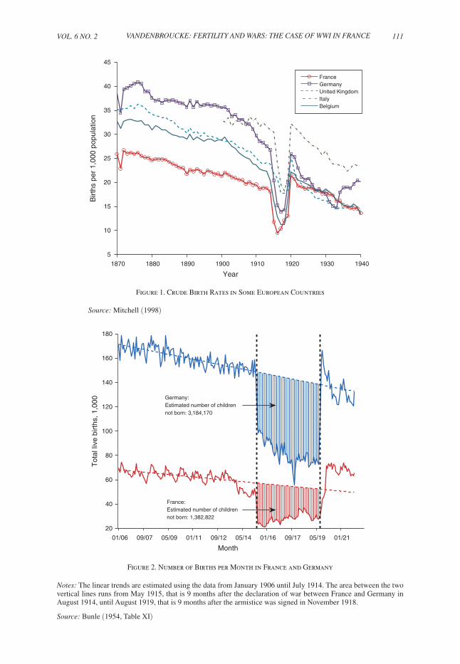
Equation (6) also helps to understand two effects of a war: the contemporaneous drop of the birth rate and the postwar catch-up. To see this, I assimilate a war to a negative income shock that lowers consumption and, therefore, raises the marginal cost of children. This implies a drop of the birth rate as illustrated in Figure 8. Such a low birth rate implies that, in the period following a war, a still-fertile household has a low stock n of children. Thus, the marginal utility of children is high and the birth rate increases. This is illustrated in Figure 9.

There are differences between equation (5) and equation (6), though. This is because children remain in the household beyond the period of their birth, yielding utility and being costly at the same time. The net, present value of these effects is measured in equation (5) by the term β ν W j+1, τ, 2 (a′, n′ ). Another difference between equations (5) and (6) pertains to the right-hand side. Since a household values con-sumption per member, it is the marginal utility of consumption per member that measures the cost of resources, hence the term u 1 (c/ϕ(n + b, 2))/ϕ(n + b, 2). In addition a newborn requires a share of consumption, hence, the term c/ϕ(n + b, 2) × ϕ 1 (n + b, 2).

b

Mar

gina

l util

ityV1(n + b)

U1(cwar)γwfτ+j‒1 U1(c)γwf

τ+j‒1

Figure 8. The Contemporaneous Decline in Fertility Caused by a War

Note: In a war, consumption is low, increasing the marginal cost of children.


To sum up, the effects discussed above are at the core of the model’s ability to generate a downward trend in the birth rate, punctuated by a negative response of births to the war and a rebound in the period following the war.

B. The War and Its Aftermath

In this section, I introduce, formally, the notion of a war in the model. This is important for the quantitative exercise of Section III. As will transpire later, the size of the income effect associated with the war is determined, to a large extent, by the likelihood of a husband dying in war. This section introduces the apparatus for this discussion.

I start by defining ω t ∈ { peace, war} to denote the state of the world. I also define z j, τ ∈ {1, 2} as the number of adults in an age-j household. Both ω t and z j, τ are random variables. Their realizations are observed at the beginning of a period, before any decisions are made.

I make the following assumptions about the distribution of ω t and z j, τ . In peace, a war is not anticipated. In war, the probability of peace next period is denoted by q. In peace, the number of adults in a household is constant. In war, the probability of a husband dying is denoted by p. I abstract from the possibility of remarriage, i.e., z j, τ = 1 is an absorbing state. Finally, I maintain the assumption that z 1, τ = 2, that is a newly formed household comprises two adults.

b

V1(n + b) V1(npost war + b) U1(c)γwfτ+j‒1

Mar

gina

l util

ity

Figure 9. The Post-War Catch Up in Fertility

Note: After a war, the stock of children is low, increasing the marginal utility of children.


A household’s optimization problem writes now,

(7) W j, τ (a, n; z, ω) = max c, a′, b

u ( c _ ϕ(n + b, z)

) + θV(n + b)

+ β E [ W j+1, τ (a′, n′; z′, ω′ )],

subject to

(8) c + a′ + γ w τ+j−1 f (ω)( n j, τ + b j, τ )

= { w τ+j−1 m (ω) + w τ+j−1

f (ω) + a/β

w τ+j−1

f (ω) + a/β

z = 2

z = 1,

where E is the expectation operator. The problem is subject to the additional restric-tion that a 1-adult household cannot have children. Note that if there is a war in the current period and the husband survives it, the probability that he does not survive the next period is (1 − q)p.

I complete the problem with a description of the relationship between wages and the state of the world, w t

i (ω). I assume, that wages drop by a proportion π i during the war, remain constant as long as the war continues, and grow by the constant fac-tor g post war > g when peace returns. Formally,

(9) w t+1 i (peace) = w t

i (peace) × { g g post war

before the war

after the war

in peace, and

(10) w t i (war) = (1 − π i ) × w last period before war i

(11) w t+1 i (peace) = g post war × w t

i (war)

in war. Note that, in peace, the probability of a war is zero. Hence, w t i (war) is not

defined in peace time.This optimization problem subsumes the benchmark model as a special case.

Namely, if a war never occurs, the choices of any generation of households are the same as they would be in the benchmark model. This derives immediately from the assumption that households do not anticipate a war and that the number of adults in a household remains constant in peace time.

The first-order conditions are similar to that of the benchmark model. For births, this is true only for households with two adults, since I assume that a 1-adult house-hold cannot have children. The first-order condition for b j, τ becomes

(12) θ V 1 (n + b) + β ν E [ W j+1, τ, 2 (a′, n′; z′ ω′ )]

= u 1 ( c _ ϕ(n + b, 2)

) 1 _ ϕ(n + b, 2)

( γ w τ+j−1 f (ω) + c _

ϕ(n + b, 2) ϕ 1 (n + b, 2) )


for j = 1, 2. The interpretation of equation (12) is similar to that of equation (5).I describe now the effects of p, q, π i , and g post war . An increase in p, the probabil-

ity of a husband dying in war, amounts to a negative expected income shock. The household reduces its consumption, and, as discussed in Section IIA, this leads to a decrease in births. A decrease in q, the probability of peace next period, acts in a similar way since it makes it more likely that the husband will die, if not in this period in the next. Note, however that a decrease in q also makes it less likely for the household to be able to postpone giving birth until peace returns. Thus, q has ambiguous effects on births. The parameter π m yields a contemporaneous, negative income effect. The parameter π f yields contemporaneous income and substitution effects. The effect of faster growth after the war, g post war , depends also on income and substitution effects. Consider the (empirically relevant) case where the substitu-tion effect dominates. Then households are induced to have children earlier. This dampens the decline in births during the war.

III. Quantitative Analysis

A. calibration of the Benchmark Model

In this section, I calibrate the model to pre-WWI data for France. I treat this period as being without wars. Several of the model’s parameters are chosen a priori. Others are chosen to minimize the distance between the time series of the actual and the predicted birth rate.

A period in the model corresponds to five years in the data. Thus, an age-1 indi-vidual in the model corresponds to a child between the age of 0 and 5 in the data. I choose ν so that the expected duration of childhood is four periods.13 This choice implies ν = 0.80. Households live for J = 7 periods.

I let the rate of interest on the risk-free asset be 4 percent per year. This implies a subjective discount factor β = 1.04⁻5. I use the rate of growth of the Gross National Product per capita in the nineteenth century, 1.6 percent per year, for the growth rate of wages.14 This implies g = 1.016 5. I normalize the initial condition ( corresponding to 1806 in the data) for w m to 1 and I assume a constant gender gap in wages, w f / w m . Huber (1931, 932–935) reports figures for the daily wages of men and women in agriculture, industry, and commerce in 1913. In industry, a woman’s wage in 1913 was 52 percent of a man’s. In agriculture, the gap was 64 percent, and in commerce it was 77 percent. Since commerce was noticeably smaller than agricul-ture and industry I use w f / w m = 0.6. In Section IIID, I present sensitivity results with respect to w f / w m .

13 The probability that a children remains in the household for one more period is ν until age six. At age seven this probability is 0. Hence, the expected duration of childhood is ∑ j=1

6 j ν j−1 (1 − ν) + 7 ν 6 .

14 See Tables 1.1 and 2.3 in Carré, Dubois, and Malinvaud (1976).


For ϕ, the adult-equivalent scale, I use the “OECD-modified equivalence scale,” which assigns a value of 1 to the first adult member in a household, 0.5 to the second adult, and 0.3 to each child:

ϕ(n, m) = 1 _ 2 + m _

2 + 0.3n.

I now turn to the remaining parameters, α ≡ (σ, θ, ρ, γ). I construct a time series of the French birth rate using the crude birth rate, that is the number of births per population, and the proportion of women between the age of 15 and 44 from Mitchell (1998). Let f t denote this data. I compute the birth rate in the model as an equally weighted average of the birth rate of age-1 and age-2 women at date t:

f t (α) = b 1, t (α) + b 2, t−1 (α)

__ 2 .

I adopt this specification for simplicity. The actual birth rate is, in fact, weighted by the relative size of each generation. French data show these weights to be remark-ably stable—about 50 percent—in the nineteenth century.15 In the model, however, declining birth rates imply counterfactual predictions for the growth rate and age composition of the population, unless exogenous trends in life expectancy and possibly migration are taken into account.16 Such additions would complicate the model while being orthogonal to the issue studied. Thus, using the observed weights of 50 percent appears to be a reasonable simplification that is also consistent with the data. Formally, I solve the following minimization problem:

(13) min α ∑ t∈

[ f t (α) − f t ] 2 + [ γ ( b 1,1906 (α) + b 2,1906 (α)) − 0.1 ] 2 ,

where is an index set: = {1806, 1811, 1816, … , 1906}. The second part of the objective function is the distance between the time spent by the 1906 generation raising its children and its empirical counterpart, 10 percent. The latter figure comes from Table II in Aguiar and Hurst (2007). They report that in the 1960s a woman in the United States spends close to six hours per week on various aspect of childcare,

15 Table A2 in Mitchell (1998) reports data showing that the ratio of women aged 25–29 to women aged 20–29, for example, is remarkably stable, about 50 percent, between 1851 and 1911. The same results hold for the 30–34 group relative to the 25–34 and other groups.

16 Let p j, τ denote the age-j adult population of generation τ. Assuming that children become adults in one period implies that the age-1 adults of generation τ + 1 are born from age-1 and age-2 adults in the previous period. That is, from generation τ and τ − 1. Thus, p 1, τ+1 = p 1, τ b 1, τ + p 2, τ−1 b 2, τ−1 . Dividing by p 1, τ yields

p 1, τ+1

_ p 1,τ = b 1, τ + p 2, τ−1

_ p 1, τ b 2, τ−1 .

Note the terms p 1, τ+1 /p 1, τ and p 2, τ−1 /p 1, τ . The first is the growth rate of population, namely the growth rate of the age-1 adult cohort. The second is the old-to-young adult ratio at date τ. In the French data these quantities exhibit no trends during the nineteenth century, while b 1, τ and b 2, τ−1 decrease. The equation above is inconsistent with this observation. It follows that the model cannot fit at the same time the decline in birth rates, the stable growth rate of population, and its stable age composition, without additional determinants of population dynamics.


that is primary, educational, and recreational. This amounts to 10 percent of the sum of market work, nonmarket work, and childcare (61 hours).

Although the parameters in α are chosen simultaneously, some aspects of the objective functions are more important for some parameters than others. The slope of the birth rate in the data is critical for the respective strength of the income and substitution effects controlled by σ and ρ. The level of the birth rate is critical for the determination of θ. Finally, γ is set to imply that the time spent by a women on childcare, on the eve of the war, is 10 percent. In Section IIID, I present sensitivity results with respect to the target figure for the time cost of raising children.

I motivate the above calibration strategy as follows. The model predicts a decline of the birth rate as wages grow only if the income effect is dominated by the sub-stitution effect (see Section II). Thus, the downward trend in the times series of the birth rate restricts the size of the income effect. The logic of the experiment that I propose is to use this discipline to assess the effect of a particular income shock, the war.

The calibrated parameters are displayed in Table 1. Figure 10 displays the computed and actual birth rate for the prewar period. Note that, by construc-tion, the parameters of the model imply an elasticity of birth rate to income of ln(100/160)/ln(1.01 6 100 ) = −0.28, since the birth rate declines from about 160 to 100 in the century before the war. This figure is within the range of estimates cen-tered around minus one-third reported by Jones, Schoonbroodt, and Tertilt (2011, Table 1) for cross-sectional data in the United States. Unfortunately, although there exist detailed births statistics by regions for France during the nineteenth century, no cross-sectional income statistics are available.

B. Baseline Experiment

parameters representing the War.—I assume that the war breaks out in 1916 and lasts for one single period. That is, the realized values of ω are ω t = peace for all t ≠ 1916, and ω 1916 = war. I consider three values for the probability that the war ends after one period: q ∈ {1.0, 0.9, 0.8}.

I calibrate p, the probability that a wife is alone after one period of war as

p = military losses of World War I

___ total men mobilized

.

Table 1—Calibration

Preferences β = 1.0 4 −5 , θ = 0.216, ρ = 0.644, σ = 0.815

Wage w m = 1, w f = 0.6 for initial (1806) generation

g = 1.0165

Cost of children γ = 1.01

Adult equivalent scale ϕ (n, m) = 1/2 + m/2 + 0.3n

Demography J = 7, ν = 0.805


There were 1.4 million military losses and 8.5 million men were mobilized. This implies p = 1.4/8.5 = 0.16. This figure is not perfect. On the one hand, it may exaggerate the risk for a wife since remarrying was possible. On the other hand, it may underestimate the risk since not all mobilized men were exposed to combat. Also, a husband may survive the war but come home disabled.17 In Section IIID, I present sensitivity results with respect to p to address these concerns.

I now turn to the calibration of π m , π f , and g post war . Figure 11 shows a 30 percent decline of output per worker in France between 1913 and 1919, followed by an annual rate of growth of 2.5 percent from 1919 to 1930. Thus, I use π f = 0.3 to represent the drop in productivity of a wife, and g post war = 1.02 5 5 . When a man is mobilized he does not work, so the husband’s wage is interpreted as a transfer to the household with a mobilized husband—a compensation. Downs (1995) reports compensations amounting to somewhere between 35 and 60 percent of a man’s pre-war salary in agriculture or industry.18 I use π m = 0.5.

Discussion of results.—The main results of this experiment are three-fold. The birth rate decreases noticeably during the war because fertile households choose to have less children. Once the war is over, that is in 1921 in the model, there is a

17 In the case of WWI this was a distinct possibility since the massive use of artillery and gases made this conflict quite different from any other conflict before. Huber (1931, 448) reports 4.2 million wounded during the war, half of the men mobilized. The number of invalid was 1.1 million among which 130,000 were mutilated and 60,000 were amputated.

18 See Downs (1995, 49) and Huber (1931, 932–935).

1800 1820 1840 1860 1880 1900 1920 1940

40

60

80

100

120

140

160

180

Year

Birt

hs p

er 1

,000

fert

ile w

omen

DataModel

Figure 10. Birth Rate, Calibration of Benchmark Model


rebound of the birth rate because the still fertile households catch up. Finally, life-time fertility is reduced for the generations exposed to the war during their fertile years.

I now describe these results in more details for the case of q = 1, that is when households expect the war to last only one period. Figure 12 shows the time path of the birth rate. Table 2 summarizes the results. In 1916, the birth rate predicted by the model falls by 45 percent relative to 1911, versus a 49 percent fall in the data. Thus, the model accounts for 91 percent of the data (45/49 = 0.91).

In 1921, the birth rate is 123 percent above its 1916 value in the model. The corresponding figure in the data is 118 percent. Thus, the model over predicts by 4 percent the postwar increase. To interpret this result, Figure 13 plots birth rates by age, conditional on a husband being in the household. Households without husbands have zero births. Consider first the 1911 cohort. In 1911 it is age 1 and does not anticipate the war. So its age-1 birth rate is on trend. In 1916 it is age 2. There is a stock of already-born children, but the war is on. It is then forced to reduce its birth rate to bear the cost of the already existing children.

Consider now the 1916 cohort. It reduces its age-1 birth rate in 1916 because its current and expected income is low. In 1921, if the husband survives, its birth rate does not return to trend though. It is above trend because the stock of children in the household is “abnormally” low, and therefore the marginal utility of a birth is high. Hence, the birth rate is high as well. Note that this effect is mitigated in the overall

1895 1900 1905 1910 1915 1920 1925 1930 1935

90

100

110

120

130

140

150

160

170

1896

= 1

00

1913

1919

Year

Figure 11. Index of Output per Worker in France, 1896–1935

source: The data is from CEPII. It is available upon request or can be downloaded at: http://www.cepii.fr/francgraph/bdd/villa/serlongues/crois.xl

http://www.cepii.fr/francgraph/bdd/villa/serlongues/crois.xl


birth rate since a fraction p of husbands in this generation died. Indeed, the overall birth rate for 1921 is computed as

b 1,1921 + (1 − p) b 2,1916

__ 2 .

It transpires from the results that the effect of p is dominated by the increase in b 2,1916 .

1800 1820 1840 1860 1880 1900 1920 1940

40

60

80

100

120

140

160

180

Year

Birt

hs p

er 1

,000

fert

ile w

omen

Data

Model

Figure 12. Birth Rate, Baseline Experiment (q = 1)

Table 2—Change in the Birth Rate in Experiments ( percent)

q = 1 q = 0.9 q = 0.8

1911–1916 1916–1921 1911–1916 1916–1921 1911–1916 1916–1921

Data −49 +118 −49 +118 −49 +118

Baseline experiment −45 +123 −45 +126 −46 +129Baseline/data 0.91 1.04 0.92 1.07 0.93 1.09

counterfactual Experiments1 – war with only p −45 +97 −45 +99 −45 +100 exp. 1/baseline 1.00 0.79 1.00 0.79 0.99 0.78

2 – war with only π m −19 +28 −19 +27 −19 +27 exp. 2/baseline 0.42 0.23 0.41 0.22 0.41 0.21

3 – war with only π f +12 −5 +13 −5 +13 −5 exp. 3/baseline −0.28 −0.04 −0.28 −0.04 −0.28 −0.04

4 – war with only g post war +4 −10 +3 −9 +3 −8 exp. 4/baseline −0.08 −0.09 −0.07 −0.07 −0.06 −0.06


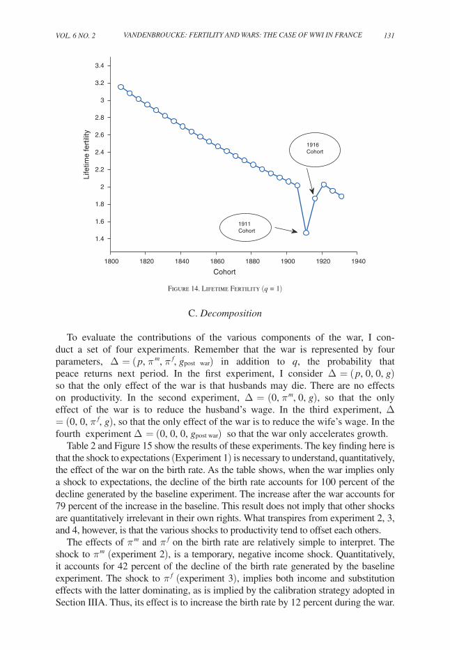
Figure 14 shows lifetime fertility by cohort.19 Two points are worth mentioning. The 1911 cohort reduces its lifetime fertility the most. This is because, even though its birth rate is on trend at age 1, it is forced to reduce it noticeably at age 2. The 1916 cohort reduces its lifetime fertility, but less. This is because the decrease during the war is compensated by the increase in 1921.

I now make a few additional observations about the results. First, Table 2 shows cases where households expect that the war continues with some probability, that is q < 1. The results are close to those discussed here. This is because there are two offsetting effects of a decrease in q. On the one hand, a decrease in q magnifies the risk associated with the war and, therefore, exacerbates the adjustment of the birth rate. On the other hand, when a young household expects the war to be over in the next period, it has an incentive to reallocate births into the future. This incentive is weakened by increases in the probability that, in the future, the war can still be on. Second, the postwar birth rate is briefly above trend because productivity is still below trend immediately after the war. The postwar birth rate, however, declines fast because of the faster growth rate in productivity. Third, Figure 13 shows that age-1 households have an above-trend birth rate after the war, while age-2 households have a below-trend birth rate. This results from faster growth again. Future children appear relatively costlier to postwar generations than to prewar generations. Hence, the shift of births toward younger age.

19 That is, for cohort τ, the figure plots ( b 1, τ + b 2, τ ) × 5, where the multiplication by five follows from the fact that a model-period is five years, while the level of births is matched to the annual birth rate.

1800 1820 1840 1860 1880 1900 1920 1940

0

50

100

150

200

250

Year

Birt

hs p

er 1

,000

fert

ile w

omen

1911Cohort

1916Cohort

Age 1Age 2

Figure 13. Age-Specific Birth Rates for Women in 2-Adult Households (q = 1)


C. Decomposition

To evaluate the contributions of the various components of the war, I con-duct a set of four experiments. Remember that the war is represented by four parameters, Δ = ( p, π m , π f , g post war ) in addition to q, the probability that peace returns next period. In the first experiment, I consider Δ = ( p, 0, 0, g) so that the only effect of the war is that husbands may die. There are no effects on productivity. In the second experiment, Δ = (0, π m , 0, g), so that the only effect of the war is to reduce the husband’s wage. In the third experiment, Δ = (0, 0, π f , g), so that the only effect of the war is to reduce the wife’s wage. In the fourth experiment Δ = (0, 0, 0, g post war ) so that the war only accelerates growth.

Table 2 and Figure 15 show the results of these experiments. The key finding here is that the shock to expectations (Experiment 1) is necessary to understand, quantitatively, the effect of the war on the birth rate. As the table shows, when the war implies only a shock to expectations, the decline of the birth rate accounts for 100 percent of the decline generated by the baseline experiment. The increase after the war accounts for 79 percent of the increase in the baseline. This result does not imply that other shocks are quantitatively irrelevant in their own rights. What transpires from experiment 2, 3, and 4, however, is that the various shocks to productivity tend to offset each others.

The effects of π m and π f on the birth rate are relatively simple to interpret. The shock to π m (experiment 2), is a temporary, negative income shock. Quantitatively, it accounts for 42 percent of the decline of the birth rate generated by the baseline experiment. The shock to π f (experiment 3), implies both income and substitution effects with the latter dominating, as is implied by the calibration strategy adopted in Section IIIA. Thus, its effect is to increase the birth rate by 12 percent during the war.

1800 1820 1840 1860 1880 1900 1920 1940

1.4

1.6

1.8

2

2.2

2.4

2.6

2.8

3

3.2

3.4

Cohort

Life

time

fert

ility

1911Cohort

1916Cohort

Figure 14. Lifetime Fertility (q = 1)


The (gross) growth rate g post war (experiment 4), on its own, tends to raise the birth rate during the war and to reduce it in 1921. This is because an increase in the growth rate raises the cost of having children late in life. Thus, in 1916, when steeper wage profiles are expected, age-1 households increase their current birth rate at the expense of their age-2 birth rate. In an experiment were g post war = g, but all the other shocks are as in the baseline experiment, that is Δ = ( p, π m , π f , g), I find that the model accounts for 94 percent of the decline during the war and overpredicts the postwar increase by 5 percent. In this experiment, unlike in the baseline, the postwar birth rates of both age-1 and age-2 households are above their prewar trends. In sum, even though the growth rate of wages matter for the timing of births, its effect on the overall birth rate are quantitatively smaller than that of other exogenous variables.

To conclude, despite the fact that the shock to expectations is the main driver of the results, changes to expected household income is not enough to predict the effect of the war on the birth rate. In the baseline experiment, the expected income of an age-1 household in 1916 is 45 percent less than it would have been if the war had not broken out. In experiment 1, which yields a similar response of the birth rate, the household’s expected income only drops by about 8 percent. The reason for this is that changes to the household’s expected income in the baseline experiment masks mutually offsetting effects that are absent in experiment 1.

D. sensitivity

I consider alternative values for (i) the probability that a woman remains alone after the war, p; (ii) the magnitude of the husband’s income loss during the war, π m ;

1800 1820 1840 1860 1880 1900 1920 1940

40

60

80

100

120

140

160

Year

Birt

hs p

er 1

,000

fert

ile w

omen

BaselineExperiment 1Experiment 2Experiment 3Experiment 4

Figure 15. Birth Rate, Counterfactual Experiments (q = 1)


(iii) the time cost of raising children, γ ; and (iv) the gender wage gap in earnings, w f / w m . Table 3 reports the results of this analysis for the case where q = 0. The main lesson to take away from this exercise is that even with noticeable changes in parameters’ value, the model generates sizeable changes in the birth rate during and after the war.

Setting the probability that a woman is alone after the war to 10 percent instead of the baseline value of 16 percent yields a 33 percent decline in the birth rate. This accounts for 67 percent of the actual decline instead of 91 percent in the baseline. An interpretation of this experiment is that it is an indirect way of accounting for the remarriage option that war widows had but that the model abstracts from. When p = 20 percent, the decline in the birth rate is more pronounced than in the baseline: 49 percent. Turning to π m : when π m = 0.75 instead of the baseline value of 50 per-cent, a household receives only a quarter of its husband prewar income as a compen-sation during the war. This exacerbates the effect of the war; the birth rate declines by 53 percent, over-predicting the actual decline by 8 percent. When π m = 0.25, the decline in the birth rate is 42 percent. It is interesting to note that the results are more sensitive to changes in p than π m . A change in p by a factor of 2 yields a 50 percent increase in the birth rate decline predicted by the model. Changing π m by a factor of 3 yields a 26 percent difference in the results. This is a reassuring result since π m is a parameter that is difficult to gauge, the only source I used being Downs (1995).

Finally, I note that in the experiments where the gender wage gap and the time cost of a child differ from the baseline, the model is recalibrated to the time series of the birth rate. It may appear “counterintuitive” that the effect of the war on the birth rate is not exacerbated when the cost of a child is larger than in the baseline, e.g., when it is 15 percent instead of 10 percent. The reason for this result is that, as the target figure for the time cost of a child changes, other parameters change too. In par-ticular, a larger-than-baseline time cost of children implies a higher value for ρ. This can be understood as follows. As the opportunity cost of raising a child increases, the marginal cost increases too. Since the model is calibrated to fit the birth rate data, marginal cost and marginal benefit must be equalized at the same birth rate level. This implies that the marginal benefit of a child must also increase, which is achieved through higher values for ρ and θ. Thus, on the one hand households

Table 3—Change in the Birth Rate in Sensitivity Analysis with q = 1 ( percent)

1911–1916 1916–1921

Data −49 +118

Baseline −45 +123

p = 0.10 −33 +80p = 0.20 −49 +144

π m = 0.25 −42 +110 π m = 0.75 −53 +165

Time cost of children: 5 percent −20 +31Time cost of children: 15 percent −40 +95

w f / w m = 0.65 −38 +84 w f / w m = 0.55 −43 +99


have an incentive to reduce their birth rate more than in the baseline during a war because children are costlier, but on the other hand, since the marginal utility of a child is higher, reducing the birth rate is also costlier than in the baseline. These two opposing effects almost offset each other when the time cost of raising a child is 15 percent.

IV. Conclusion

The human losses of WWI were not only on the battlefield. In France, the number of children not born during the war was as large as military casualties. This affected the age composition of the French population for the rest of the twentieth century. I presented a theory of this phenomenon. In the model, children yield utils, but they require time to raise. The war is tantamount to an income shock, both contempora-neous and expected. I calibrated the model to the time series of the prewar birth rate. I found that the war triggered a large, negative response of the birth rate, account-ing for 91 percent of the observed decline. The model also features a mechanism to account for the postwar rebound in the birth rate. Its calibrated version overpredicts this rebound by 4 percent.

The key determinant of these results is the loss of expected income associated with the risk that a wife remains alone after the war. The war also features temporary shocks to wages for both husband and wives, but these forces tend to offset each other.

Although the analysis that I presented is about France during the WWI, neither France nor WWI are unique cases. As is clear from Figure 1, other belligerents of the war experienced the same fate as France. Furthermore, there is evidence, presented by Caldwell (2004), that birth rates declined in many countries during various episodes of wars, civil wars, revolutions, and dictatorships (see Table 4). The conclusions that I reach in this analysis could be extended to these episodes in future research.

Vol. 6 No. 2 135Vandenbroucke: fertility and wars: the case of wwi in france

REFERENCES

Abramitzky, Ran, Adeline Delavande, and Luis Vasconcelos. 2011. “Marrying Up: The Role of Sex Ratio in Assortative Matching.” American Economic Journal: Applied Economics 3 (3): 124–57.

Aguiar, Mark, and Eric Hurst. 2007. “Measuring Trends in Leisure: The Allocation of Time Over Five Decades.” Quarterly Journal of Economics 122 (3): 969–1006.

Albanesi, Stefania, and Claudia Olivetti. 2010. “Maternal Health and the Baby Boom.” National Bureau of Economic Research (NBER) Working Papers 16146.

Barro, Robert J., and Garry S. Becker. 1989. “Fertility Choice in a Model of Economic Growth.” Econometrica 57 (2): 481–501.

Becker, Gary S. 1960. “An Economic Analysis of Fertility.” In Demographic and Economic Change in Developed Countries, 209–40. New York: Columbia University Press.

Becker, Gary S., and Robert J. Barro. 1988. “A Reformulation of the Economic Theory of Fertility.” Quarterly Journal of Economics 103 (1): 1–25.

Bunle, Henry. 1954. le mouvement naturel de la population dans le monde de 1906 a 1936. Paris: Les editions de l’INED.

Caldwell, John C. 2004. “Social Upheaval and Fertility Decline.” Journal of Family History 29 (4): 382–406.

Carré, Jean-Jacques, Paul Dubois, and Edmond Malinvaud. 1976. French Economic Growth. Stan-ford, CA: Stanford University Press.

Doepke, Matthias, Moshe Hazan, and Yishay Maoz. 2007. “The Baby Boom and World War II: A Mac-roeconomic Analysis.” National Bureau of Economic Research (NBER) Working Paper 13707.

Downs, Laura Lee. 1995. Manufacturing Inequality: Gender Division in the French and British Met-alworking Industries, 1914–1939. Ithaca, NY: Cornell University Press.

Festy, Patrick. 1984. “Effets et répercussion de la première guerre mondiale sur la fécondité française.” Population 39 (6): 977–1010.

Galor, Oded, and David N. Weil. 2000. “Population, Technology, and Growth: From Malthusian Stag-nation to the Demographic Transition and Beyond.” American Economic Review 90 (4): 806–28.

Table 4 — Change in the Crude Birth Rate in Social Upheavals ( percent)

Change in theCountry Episode Period crude birth rate

England Civil war, commonwealth, and early restoration

1641–1666 −17.3

France Revolution 1787–1804 −22.5

United States of America Civil war 1860–1870 −12.8

Russia WWI and revolution 1913–1921 −24.4

Germany War, revolution, defeat, inflation 1913–1924 −26.1

Austria War, defeat, empire dismembered 1913–1924 −26.9

Spain Civil war and dictatorship 1935–1942 −21.4

Germany War, defeat, occupation 1938–1950 −17.3

Japan War, defeat, occupation 1940–1955 −34.0

Chile Military coup and dictatorship 1972–1978 −22.3

Portugal Revolution 1973–1985 −33.3

Spain Dictatorship to democracy 1976–1985 −37.2

Eastern Europe Communism to capitalism 1986–1998 Russia −56.0 Poland −40.0 Czechoslovakia (Czech Republic) −38.0

Notes: Caldwell reports that when the birth rate was already experiencing a declining trend, the reductions observed during the periods of unrest are significantly more pronounced than before and after. For example, the Spanish birth rate fell as much during the Civil War (1935–1942) as during the 35 years before.

Source: Caldwell (2004, Table 1)


Greenwood, Jeremy, Ananth Seshadri, and Guillaume Vandenbroucke. 2005. “The Baby Boom and Baby Bust.” American Economic review 95 (1): 183–207.

Henry, Louis. 1966. “Perturbations de la nuptialité résultant de la guerre 1914–1918.” population 21 (2): 273–332.

Huber, Michel. 1931. La population de la France pendant la guerre. Paris: Les Presses Universitaires de France.

Jones, Larry E., and Alice Schoonbroodt. 2011. “Baby Busts and Baby Booms: The Fertility Response to Shocks in Dynastic Models.” National Bureau of Economic Research (NBER) Working Paper 16596.

Jones, Larry E., Alice Schoonbroodt, and Michèle Tertilt. 2011. “Fertility Theories: Can They Explain the Negative Fertility-Income Relationship?” In Demography and the Economy, edited by John B. Shoven, 43–100. Chicago: University of Chicago Press.

Knowles, John A., and Guillaume Vandenbroucke. 2013. “Dynamic Squeezing: Marriage and Fertility in France After World War One.” Unpublished.

Manuelli, Rodolfo E., and Ananth Seshadri. 2009. “Explaining International Fertility Differences.” Quarterly Journal of Economics 124 (2): 771–807.

Mitchell, Brian R. 1998. International Historical statistics: Europe, 1750–1993. New York: Stockton Press.

Robert, Jean-Louis. 2005. “Women and Work in France During the First World War.” In The upheaval of War: Family, Work and Welfare in Europe, 1914–1918, edited by Richard Wall and Jay Winter, 251–66. Cambridge, UK: Cambridge University Press.

Schweitzer, Sylvie. 2002. Les Femmes ont Toujours Travaillé: une Histoire Du Travail Des Femmes Aux XIX e et XX e siècles. Paris: Odile Jacob.

Vandenbroucke, Guillaume. 2014. “Fertility and Wars: The Case of World War I in France: Dataset.” American Economic Journal: Macroeconomics. http://dx.doi.org/10.1257/mac.6.2.108.

Vincent, Paul. 1946. “Conséquences De Six Années De Guerre Sur La Population Française.” popula-tion 1 (3): 429–40.


Documents

Fertility and Wars: The Case of World War I in Franceguillaumevdb.net/ww1_Final.pdf · Fertility and Wars: The Case of World War I in France ... Jones, Schoonbroodt, ... There were