Ferran Palero Pastor INVESTMAT MSc Thesis

UNIVERSITAT POLITÈCNICA DE VALÈNCIA

Mathematical modelling and parentage analysis of Hybrid

Zones

Ferran Palero Pastor

INVESTMAT MSc Thesis

Valencia, December 2009

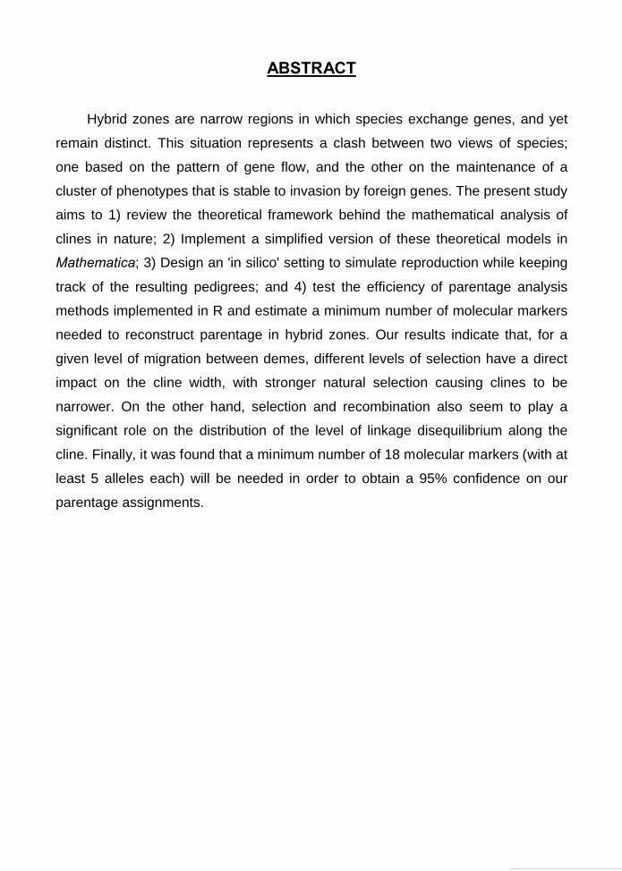
http://www.pdfonline.com/easypdf/?gad=CLjUiqcCEgjbNejkqKEugRjG27j-AyCw_-AP

ABSTRACT

Hybrid zones are narrow regions in which species exchange genes, and yet

remain distinct. This situation represents a clash between two views of species;

one based on the pattern of gene flow, and the other on the maintenance of a

cluster of phenotypes that is stable to invasion by foreign genes. The present study

aims to 1) review the theoretical framework behind the mathematical analysis of

clines in nature; 2) Implement a simplified version of these theoretical models in

Mathematica; 3) Design an 'in silico' setting to simulate reproduction while keeping

track of the resulting pedigrees; and 4) test the efficiency of parentage analysis

methods implemented in R and estimate a minimum number of molecular markers

needed to reconstruct parentage in hybrid zones. Our results indicate that, for a

given level of migration between demes, different levels of selection have a direct

impact on the cline width, with stronger natural selection causing clines to be

narrower. On the other hand, selection and recombination also seem to play a

significant role on the distribution of the level of linkage disequilibrium along the

cline. Finally, it was found that a minimum number of 18 molecular markers (with at

least 5 alleles each) will be needed in order to obtain a 95% confidence on our

parentage assignments.


RESUM

Les zones híbrides són regions estretes en les quals troben espècies que

intercanvien gens, i tanmateix romanen diferenciades. Aquesta situació representa

un enfrontament entre dues visions d'espècie; una basada en el patró de flux

gènic, i l'altra en el manteniment d'un grup d’individus amb un fenotip estable.

Aquest treball pretén 1) revisar la teoria en què es basa l'anàlisi matemàtica de

clines; 2) implementar una versió simplificada d'aquests models teòrics a

Mathematica; 3) Establir un disseny 'in silico' que permeta simular reproducció

biològica i alhora registre els pedigrís resultants; i 4) provar el rendiment dels

mètodes d'anàlisi de parentiu implementats a R i calcular un nombre mínim de

marcadors moleculars necessaris per reconstruir pedigrís en zones híbrides. Els

nostres resultats indiquen que, per a un nivell donat de migració entre localitats,

els diferents nivells de selecció tenen un impacte directe en l'amplada de la clina,

amb una selecció major resultant en clines més estretes. D'altra banda, selecció i

recombinació també semblen jugar un paper significatiu en la distribució del nivell

de desequilibri de lligament al llarg de la clina. Finalment, es troba que un mínim

de 18 marcadors moleculars (amb com >5 al·lels cadascun) són necessaris per

obtenir un 95% de confiança en les nostres assignacions de parentiu.


CONTENTS

1. Abstract 1

2. Introduction 2

3. Methods: Theoretical Framework

a. Modelling Hybrid Zones 3

b. Statistical theory of paternity inference 9

4. Analysis and results

a. Implementation of theoretical models in Mathematica:

Hybrid Zone simulations 12

b. Simulating a cline: Results 14

c. Pedigree simulations in Mathematica and Parentage analysis in R 20

5. Discussion

a. Hybrid zone simulations 25

b. Parental assignment methods 27

c. Future studies: Analysing real data from Antirrhinum 28

6. Acknowledgements 29

7. References 29


Mathematical modelling and Parentageanalysis of Hybrid Zones

Ferran Palero

Institute of Science and Technology Austria (ISTA)Am Campus 1A – 3400 KlosterneuburgAustria.e-mail: [email protected]

"It is not clear how Templeton's cohesion species differs from a biological species, although I suspect a cohesionspecies would possess additional reproductive barriers acquired during the years of deliberation on its status."(Schemske 2000)

AbstractA biological species is defined as an "actually or potentially interbreeding group of populations". In practice, any taxathat can produce viable and fertile F2 generations are regarded as being of the same species. However, hybrid zones arenarrow regions in which genetically distinct populations meet, mate and produce hybrids. Therefore, species exchangegenes, and yet remain distinct. This situation represents a clash between two views of species; one based on the patternof gene flow, and the other on the maintenance of a cluster of phenotypes that is stable to invasion by foreign genes. Inorder to explain how selection can maintain well-defined species despite gene flow, a diffusion equation approximationto hybrid zones is presented in this report. Besides representing the basis for a challenging theoretical model on geneflow-selection equilibrium, stable clines present an interesting situation for the analysis of paternity and pedigreereconstruction methods.The present study aims to 1) shortly review the theoretical framework behind the mathematical analysis of clines innature, pointing out the most relevant assumptions made by the models; 2) Implement a simplified version of thesetheoretical models in Mathematica, in order to describe the quantitative effect of different levels of dispersal andselection on the shape of the cline; 3) Design an 'in silico' setting to simulate reproduction while keeping track of theresulting pedigrees; and 4) test the efficiency of parentage analysis methods implemented in R and estimate a minimumnumber of molecular markers needed to reconstruct parentage in hybrid zones.Our results indicate that, for a given level of migration between demes, different levels of selection have a direct impacton the cline width, with stronger natural selection causing clines to be narrower. On the other hand, selection andrecombination also seem to play a significant role on the distribution of the level of linkage disequilibrium along thecline. Finally, our simulations indicate that a minimum number of 18 molecular markers (with at least 5 alleles each)will be needed in order to obtain a 95% confidence on our parentage assignments. All the analyses described in thispaper were performed using a Mathematica 7.0 notebook.

- 1 -


Introduction

Hybrid Zones : Natural Selection in actionHybrid zones are examples of stepped clines, which are dramatic geographic gradients in the frequency of a gene or atrait. One might imagine that hybrid zones are rather rare and hard to find. However, we have many examples of clinesin nature: differences in skin color in humans, differences in color pattern in the European fire-bellied toad (Bombinabombina) and the yellow-bellied toad (Bombina variegata), differences in chromosome number in Mus musculus, andmany others (Barton and Hewitt, 1985; Capanna, 1980). In fact, the present study is originally motivated by a strikingAntirrhinum hybrid zone located in the Catalonian Pyrenees (Whibley et al., 2006). The snapdragon Antirrhinum showstwo different flower colors in a very narrow area, less than 10km wide, near Planoles. As you travel along the mainroad, flowers shift from being pink on one extreme to yellow in the other, and only a few hybrids (orange flowers) canbe observed in between. In order to explain the scarcity of hybrids in this area, it has been hypothesized that orangeflowers (hybrids) are selected against by pollinators (Bumblebees: Bombus terrestris), which will make them less fertileand impede their expansion. However, several questions arise from these considerations: how strong should be naturalselection against hybrids to maintain the observed differences? To which extent does pollen dispersal (gene flow)between pink and yellow flowers influence the shape of the cline?

A biological species is defined as an "actually or potentially interbreeding group of populations". In principle, we wouldexpect gene flow and dispersal to homogenize the genetic composition of the populations in hybrid zones, but insteadthey remain distinct. How could it be? This represents a clash between two views of species; one based on the pattern ofgene flow, and the other on the maintenance of a cluster of phenotypes that is stable to invasion by foreign genes.Therefore, hybrid zones offer us several ways of understanding the nature and origin of species. The wide range ofgenotypes found in a hybrid zone can be used to analyze the genetic differences and selective forces that separate thetaxa involved. This may allow some inferences about the way these differences evolved and, by extrapolation, about theway fully isolated species diverge from each other. As will be shown in the present report, studies of hybrid zones allowus to quantify the genetic differences responsible for speciation, to measure the diffusion of genes between divergingtaxa, and to understand the spread of alternative adaptations.

A more practical reason for developing a model of gene flow and selection is to increase our understanding of thecauses of the observed spatial patterns of gene frequencies. In fact, Haldane (1948) original work on this subject (seebelow) was motivated by the problem of measuring selection in Mus musculus and has been used by others to estimatethe strength of selection in other natural population. Despite being a key concept in the Darwinian theory of evolution,estimating selection in natural conditions remains a challenging task. One of the most accessible ways to estimate thestrength of selection in nature is to measure the rate of change in gene frequencies in a cline and compare with thoseresults expected under a particular model. That is still another reason why studying hybrid zones should be a priority forevolutionary biologists.

Overview : Models of clines in continuous habitats

Several models have been proposed in order to account for the existence of clines in natural populations. The availablemodels of clines in continuous habitats can be arranged into two classes. In the first class, dispersal is negligible.Selection maintains a stable equilibrium at each locality (e.g. through heterozygote advantage). In that case, the cline

just mirrors a smooth gradient in selection coefficients and hence in the equilibrium point. We will call these dispersal-

independent clines; and they include Moore's (1977) "bounded hybrid superiority". In the second class, thehomogenizing effect of dispersal is balanced against some cause of spatial heterogeneity. Most theoretical work hasbeen on such models (Felsenstein, 1976). They include neutral clines, in which an initially steep gradient decays withtime; waves of advance of an advantageous allele (Fisher, 1937); and dispersal-selection balance, in which eitherdifferences in environment (Haldane, 1948) or selection against intermediate genotypes (heterozygotes or recombinants)(Bazykin, 1969, 1972) maintains a stable cline. We will refer to the last type as a tension (hybrid) zone.

The distinction between these two classes depends on the characteristic scale of selection, l, where l

s, with2 =

dispersal rate (more precisely, the variance in distance between parent and offspring). The selection coefficient (s) is

proportional to selection or, for a neutral cline, it is the inverse of the time since contact (Slatkin, 1973). Any dispersal-

2 MSc Hybrid Zones.nb

- 2 -


dependent cline has a width (w, defined as the inverse of the maximum gradient) of the same order as l. Conversely, if

selection is to maintain a dispersal independent cline, w must be much greater than l. A cline can still be regarded as adispersal-selection balance even if some hybrid genotypes are favored, provided they are only favored within a regionmuch narrower than l. When many clines coincide, linkage disequilibria will be generated by the dispersal of parentalcombinations of alleles into the center (Slatkin, 1975). If many genes are involved and selection is comparable withrecombination, disequilibria will induce a sharp step in each cline, flanked by long tails of introgression (see below).The central region of the cline (in which disequilibria are strong) will be distinct from the surrounding tails, and it hasbeen proposed that its width will depend strongly on the ratio between selection and recombination (Barton, 1983).

Simulating hybrid zone evolution "in silico" and Parental assignment

In 1991, Barton and Turelli developed recursions to describe the evolution of multilocus systems under arbitrary formsof selection. Later, Kirkpatrick et al. (2002) generalized their approach to allow for arbitrary modes of inheritance,including diploidy, polyploidy, sex linkage, cytoplasmic inheritance, and genomic imprinting. The framework was alsoextended to allow for other deterministic evolutionary forces, including migration and mutation. Exact recursions thatfully describe the state of the population were presented and implemented in a computer algebra package calledMULTILOCUS. The present study builds up on that work, by extending their approach to the analysis of hybrid zones.Furthermore, since we are particularly interested in analysing real data from the Antirrhinum hybrid zone, our study willinclude further simulations on pedigree construction, therefore increasing the current functionality of the package.

As previously pointed out, selection and dispersal are key factors determining the main traits of the hybrid zone, such ascline shape and width. Therefore, in order to estimate dispersal rate (or the variance in distance between parent andoffspring) and selection (or reproductive success), we should be able to trace the evolution of a biological system fromgeneration to generation, describing which individuals are able to produce viable offspring and how far from theirparents do these descendants get established. This is not an easy task, since tagging and tracking every individual in apopulation would be prohibitive. Nevertheless, recent studies indicate that polymorphic genetic markers are potentiallyhelpful in resolving genealogical relationships among individuals in a natural population (Jones and Ardren, 2003). Ourstudy will further investigate which is the minimum number of molecular markers needed in order to have highconfidence on our paternity estimates.

Aims

In summary, the present study aims to 1) shortly review the theoretical framework behind the mathematical analysis ofclines in nature, pointing out the most relevant assumptions made by the models; 2) Implement a simplified version ofthese theoretical models in Mathematica, in order to describe the quantitative effect of different levels of dispersal andselection on the shape of the cline; 3) Design an 'in silico' setting to simulate reproduction while keeping track of theresulting pedigrees; and 4) test the efficiency of parentage analysis methods in reconstructing the simulated pedigrees.

Methods: Theoretical Framework

Modelling Hybrid Zones

Quick introduction to genetics jargon

We now give a brief explanation of some of the biological and genetical terms used. These definitions may not beentirely comprehensive, however they are adequate for the purposes of this thesis. Unless stated otherwise, we consider

a diploid population, so that each individual possesses two sets of chromosomes, one set inherited from each parent. Weare only interested in the genes located at one particular locus (i.e. the genes at a particular place on a particular

chromosome). We consider the situation in which the gene occurs in two different forms, called alleles. The Mendelianmodel of inheritance assumes that parents pass on discrete heritable units - genes - that remain separate and can bepassed on to subsequent generations in undiluted form.

The genetic makeup of an individual is known as its genotype. A homozygote possesses two identical alleles for agiven trait, whereas a heterozygote has two different alleles for a given trait. The physical traits exhibited by anindividual is known as its phenotype. In a heterozygote, the allele that is fully expressed by the phenotype is known as

the dominant allele, whereas if an allele is completely masked in the phenotype, it is known as recessive. A change in

MSc Hybrid Zones.nb 3

- 3 -


the gene frequencies in a population is the most elementary step in evolution from a population genetics point of view.Variation exists in a population due to the different possible alleles an individual may possess, and this variation isheritable. According to the Darwinian theory of natural selection, individuals with variations that are best suited to theenvironment are more likely to survive and pass on their advantageous genes to successive generations.Biologists hope to determine the probability of the ultimate success of an advantageous gene by attempting to modelthese changes in allele frequencies. In order to do so, population genetics uses some deterministic models that havegreat similarities with those used in other disciplines. In this thesis we will focus particuarly on diffusion equationsapplied to the analysis of hybrid zones.

The Diffusion equation in population genetics : "Fisher's Wave of Advance".

The origins of the application of a diffusion approximation in population genetics are to be found in the pioneering workof Fisher (1930, 1937). He considered the case of a population distributed in a linear habitat, such as a shoreline, whichis occupied with uniform density. If at any point of the habitat an advantageous mutation occurred, we would expect themutant gene to increase at the expense of the alleles previously occupying the space around the new mutant. Thisprocess will later, as the advantageous gene is diffused into the surrounding population, expand in the adjacent portionsof its range. Supposing the range to be long compared with the distances separating the sites of offspring from those oftheir parents, there will be, advancing from the origin, a wave of increase in the gene frequency.

Let p be the frequency of the mutant gene, and q that of its parent allele, which we shall suppose to be the only otherallele present. Let s be the intensity of selection in favour of the mutant gene, supposed independent of p. If we furthersuppose that the rate of diffusion per generation across any boundary may be equated to

(1)kp

x

at that boundary, x being the coordinate measuring position in the linear habitat, then the allele frequency of the mutantallele p must satisfy the differential equation:

(2)p

t k

2 p

x2 spq

where t stands for time in generations.

Notice that we are stating that the rate of change in allele frequency through time equals the sum of the allele frequencychange through space due to diffusion plus the amount due to selection. This will become important later.

The constant k is a coefficient of diffusion analogous to that used in physics. Its use should be appropriate in manycases. Of course, in all real cases we may expect irregularities due to k varying at different points of the range, due tovariations in the density of the population, and to variation in the selective advantage of the mutant at different places.Further, the means of diffusion may involve an unequal drift in opposite directions (anisotropy), so that some parts ofthe range predominate as centres of production and others as centres of extinction. Nevertheless, the purpose ofequation (1) is to specify the simplest possible conditions.

If we seek for a solution representing a wave of stationary form advancing with velocity v, we may put

(3)p

t v

p

x

and obtain the differential equation (2) involving only one independent variable:

(4)kd2p

dx2 v

dp

dx spq 0

Since the variable x does not appear explicitly, we may define, for the frequency gradient,

(5)g dp

dx

which allows us to write


- 4 -


(6)d2p

dx2

dg

dx g

dg

dp

and therefore find the relation between the frequency gradient (g) and the mutant allele frequency (p),

(7)kdg

dp vg spq 0

At the point of inflexion, we will havedg

dp 0, and vg = spq; in advance of this point

dg

dp 0.

If the ratio between the frequency gradient and the mutant allele frequency tends to a limit value when p tends to zero

(8)limp0

g

p u

then u must satisfy the equation

(9)ku2 vu s 0

which is a quadratic equation in u that has real roots only if v2 is not less than 4ks. Notice thatg

p cannot tend to zero for

vg > spq, and cannot tend to infinity because v kdg

dp. Therefore, solutions only exist for which the velocity of

propagation is equal to, or exceeds, 2 ks .

The most striking point about equation (4) is that the velocity of advance of the mutant factor appears to beindeterminate. If, for example, any part of the range were filled with the mutant form, and the zone of transition wereartificially given frequencies with the low gradient of gene ratio appropriate to a high velocity, the mutation wouldspread with a higher velocity than if the initial gradient had been higher, and would continue to spread indefinitely withthis higher velocity so long as uniform conditions were encountered.

Ultimately, the velocity of advance would adjust itself so as to be the same irrespective of the initial conditions. If this isso, equation (4) must omit some essential element of the problem, and it is indeed clear that while a coefficient ofdiffusion may represent the biological conditions adequately in places where large numbers of individuals of both typesare available, it cannot do so at the extreme front and back of the advancing wave, where the numbers of the mutant andthe parent gene respectively are small, and where their distribution must be largely sporadic. This reasoning indicatesthat the diffusion approximation would not be aplicable under boundary conditions.

Fisher further defined the effect of chance at the advancing front, which he calculated by considering an aggregate ofdiscrete particles, which increase in number with a relative growth rate s, as at the wave front of our original problem,but are free also to increase in numbers indefinitely in the interior of their range. We shall suppose them to be scatteredat small unit intervals of time so that the displacement of the particles at each scattering are is independent and normallydistributed

(10)Nx, 1

2

12 x2

2 dx

where k of our previous notation will correspond to 2

2.

Finally, the indeterminacy of velocity can be resolved by comparison with the properties of multiplying aggregates ofparticles, constantly subjected to random scattering. It appears that the actual velocity of advance must be the minimumcompatible with the differential equation. This velocity is proportional to the square root of the intensity of selectiveadvantage and to the standard deviation of scattering in each generation, or to the square root of the diffusion coefficientwhen time is measured in generations.

It may be expressed in the form

(11)v 2s 2 ks


- 5 -


where, again, s is the selectivc advantage, the standard deviation of scattering, and k the diffusion coefficient.

The "length" of the wave, or the distance between any two assigned gene ratios, is proportional to ks

, wich may

be taken as the unit of length.In summary, Fisher considered a favorable mutant arising in a continuously distributed population and presented apartial differential equation for the deterministic change in the geographic pattern of gene frequencies. Equation (2)predicts a wave front of rising gene frequencies propagating through the population and leaving behind it a region fixedfor the favored allele. Since the allele was assumed to be favorable in all parts of the population, no stable cline is

achieved. However, it has been shown that the velocity of advance of the wave will be proportional to s , and the

length of the wave front to

s. Despite there is some indeterminacy in the shape and speed of the wave, which can

depend on the initial conditions, Fisher argued that his solution, would be the ultimate result after initial conditioneffects were lost.

Mathematical Model of a Hybrid Zone : Theory of a cline

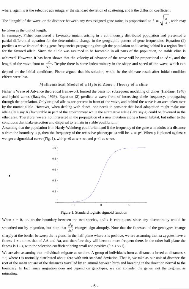
Fisher' s Wave of Advance theoretical framework formed the basis for subsequent modelling of clines (Haldane, 1948)and hybrid zones (Bazykin, 1969). Equation (2) predicts a wave front of increasing allele frequency, propagatingthrough the population. Only original alleles are present in front of the wave, and behind the wave is an area taken overby the mutant allele. However, when dealing with clines, one needs to consider that local adaptation might make oneallele (let's say A) favourable in part of the environment while the alternative allele (let's say a) could be favoured in theother area. Therefore, we are not interested in the propagation of a new mutation along a linear habitat, but rather to theconditions that make selection and dispersal to remain in stable equilibrium.Assuming that the population is in Hardy-Weinberg equilibrium and if the frequency of the gene a in adults at a distancex from the boundary is p, then the frequency of the recessive phenotype aa will be z p2. When p is plotted against x

we get a sigmoideal curve (Fig. 1), with p0 as x-, and p1 as x.

5 0 5

0.2

0.4

0.6

0.8

1.0

Figure 1. Standard logistic sigmoid function

When x = 0, i.e. on the boundary between the two species, dp/dx is continuous, since any discontinuity would be

smoothed out by migration, but note that2p

x2 changes sign abruptly. Note that the fitnesses of the genotypes change

sharply at the border between the regions. In the half plane where x is positive, we are assuming that aa zygotes have afitness 1 + s times that of AA and Aa, and therefore they will become more frequent there. In the other half plane thefitness is 1 - s, with the selection coefficient being small and positive (0 < s <<1).

We are also assuming that individuals migrate at random. A group of individuals born at distance x breed at distances x+ t, where t is normally distributed about zero with unit standard deviation. That is, we take as our unit of distance theroot of the mean square of the distances travelled by an animal between birth and breeding in the direction normal to theboundary. In fact, since migration does not depend on genotypes, we can consider the genes, not the zygotes, asmigrating.


- 6 -


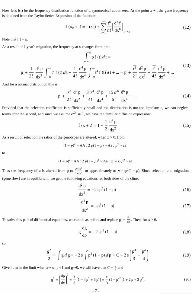
Now let's f(t) be the frequency distribution function of t, symmetrical about zero. At the point x + t the gene frequencyis obtained from the Taylor Series Expansion of the function:

(12)f x0 t f x0 n1

tn

n dnf

dxnxx0

Note that f() = p.

As a result of 1 year's migration, the frequency at x changes from p to:

(13)

p f t t

p 1

2 d2p

dx2

t2f t t 1

4 d4p

dx4

t4f t t ... p t2

2 d2p

dx2

t4

4 d4p

dx4 ...

And for a normal distribution this is

(14)p 2

2 d2p

dx2

34

4 d4p

dx4

156

6 d6p

dx6 ...

Provided that the selection coefficient is sufficiently small and the distribution is not too leptokurtic, we can neglect

terms after the second, and since we assume2 1, we have the familiar diffusion expression:

(15)f x t 1 1

2d2p

dx2

As a result of selection the ratios of the genotypes are altered, when x > 0, from:1 p2 ~ AA : 2p1 p ~ Aa : p2 ~ aa

to 1 p2~ AA : 2p1 p2 ~ Aa : 1 sp2 ~ aa

Thus the frequency of a is altered from p topsp2

1sp2, or approximately to p sp21 p. Since selection and migration

(gene flow) are in equilibrium, we get the following equations for both sides of the cline:

(16)d2p

dx2 2sp21 p

(17)d2p

dx2 sp21 p

To solve this pair of differential equations, we can do as before and replace g dpdx

. Then, for x > 0,

(18)gdg

dp 2sp21 p

so

(19)g2

2 gg 2s p21 pp C 2s

p3

3

p4

4

Given that in the limit when x, p1 and g0, we will have that C s6 and

(20)g2 dp

dx

2

s

31 4p3 3p4 s

31 p21 2p 3p2.


- 7 -


Similarly, when x < 0, g2 dpdx

2 2C' 4s p3

3

p4

4. So when x-, p0 and g0, we have C ' 0 and

(21)g2 dp

dx

2

sp3

34 3p

Now, in the middle of the cline, when x = 0, p = b anddpdx

has the same value for both branches of the cline. Hence we

gets31 4b3 3b4 s

34b3 3b4, or simplifying 3b4 4b3 1

2 0. This equation, giving the value of

the allele frequency on the middle of the cline, has one and only one root between 0 and 1, which can be found byiteration.

Mathematical Model of a Hybrid Zone : Moving into 2-dimensions

Bazykin (1969) suggested the simplest model of a tension zone, which is similar to the one that we will follow in oursimulations. In this case, we assume that heterozygotes have fitness 1 - s relative to either homozygote. If the allelefrequency is p, the change in allele frequency is then (for small s):

(22)p

t2

22 p

x2 spqp q

where p + q = 1.

Figure 2. Change in allele frequency along the cline (-100 < x < 100) at different selection levels (0.001 < s < 0.01).

As stated before, this equation describes the situation in which "the heterozygote is less fit than both homozygotes" and"homozygote fitness is equal". Again, remember that the dispersal rate is defined as the standard deviation of the

distance between parent and offspring along a chosen axis and it has units of distance time12.

Bazykin' s model is based on a special kind of reaction-diffusion equations, in which attention is centred not on thespontaneous formation of a pattern from a homogeneous field, but on the interaction between areas which have movedto different states. This particular equation has the solution:

(23)p 1

1 exx0

l


- 8 -


where l 2

2sis the characteristic distance over which selection changes allele frequencies Fig. 3,

and the cline width is 4l.

Figure 3. Change in characteristic length with dispersal (0 < < 100) and selection (0.001 < s < 0.01).

In this model, the environment is homogeneous and the homozygotes have equal fitnesses, so the cline can form

anywhere (x0), and the equation has a family of neutrally stable solutions that are known as 'topological solitons'.

Topological solitons are solitary waves set up at the boundary between two regions constrained to be in different states.The same phenomenon (often the same equation) arises in many other fields. Topological solitons are solutions ofsystems of partial differential equations representing stable structures which are localized in space, with their stabilitybeing due (in part) to non-trivial topology. Systems admitting such solitons have been known for a long time; the firstexamples were in one space dimension, whereas more recent work has concentrated on structures in two and threespace dimensions. Investigation of the mathematical properties of topological solitons has proceeded alongside thesearch for their applications in the description of numerous processes and phenomena in physics and biology.Nevertheless, their application to population genetics is very recent and mostly unexplored.

Statistical theory of paternity inferenceNow we move to a completely different topic, but that will be needed in order to get estimates of dispersal to be used inour hybrid zone model. Parentage analysis is a precise form of assignment testing that can be particularly useful fordetecting ecological and evolutionary patterns in systems with high levels of gene flow (Manel et al., 2005). Suchsystems have limited genetic differentiation, which severely restricts the utility of population-level assignment methods.Therefore, parentage analyses may allow for the inference of gene flow and dispersal at ecologically relevanttimescales.

A challenge to employing parentage analysis in natural populations is that large population sizes, variable dispersaldistances and high rates of mortality may severely constrain the number of sampled parent-offspring pairs. Thesechallenges are amplified in systems where patterns of dispersal are unobservable, such as when propagules are too smallto track directly (e.g. pollen dispersal). In addition, because of a lack of pragmatic methods, long-distance dispersalevents are often ignored or remain undetected in many species of plants (Nathan, 2006), fungi (Kauserud et al., 2006)and animals that are cryptic or have complex life histories (Derycke et al., 2008). Nevertheless, large genotypic data sets


- 9 -


may still be used to uncover some of these enigmatic processes, and parentage analysis can be a powerful tool for thedirect detection of patterns of dispersal and population connectivity. As shown in the previous section, dispersal plays akey role in defining cline behaviour and estimation of selection. Therefore, being able to assign parentage is criticalwhen dealing with hybrid zones.

Methods of parentage analysis

Several methods of parentage analysis are available in the literature. Exclusion is based on Mendelian rules ofinheritance and uses incompatibilities between parents and offspring to reject particular parent-offspring hypotheses.Categorical and fractional likelihood assign progeny to non-excluded parents based on likelihood scores derived fromtheir genotypes. The categorical technique assigns the entire offspring to a particular male, whereas the fractionaltechnique splits an offspring among all compatible males.

These methods are expected to perform differently from one another when estimating the variances in reproductive ormating success for one or both sexes in a population. Thus, the categorical method overestimates the reproductivesuccess of individuals with many homozygous loci, the fractional technique requires the researcher to set a priorprobability of parentage, etc. Moreover, although they might seem straightforward in principle, such analyses areusually complicated by several factors such as incomplete sampling of potential parents, individuals being related toeach other in ways not explicitly considered (e.g. individuals belonging to a sibship but only considered as potentialparent and offspring), and non-Mendelian transmission of genotypes (through null alleles, mutations or genotypingerror).

LOD Scores

If we sample a triplet of individuals (A, B, C) with single locus genotypes gA, gB and gC, one can compare thelikelihood of the hypothesis (H1) that the three individuals are offspring, mother and father, with the likelihood of thealternative hypothesis (H2) that the three individuals are unrelated. This comparison is usually expressed as a log-ratio,

which defines the parent-pair LOD score (e.g. Meagher and Thompson, 1986):

(24)LODgA, gB, gC logPrgA, gB, gC H1PrgA, gB, gC H2 log

TgA gB, gCPrgA

In this notation, the Mendelian transmission probability is denoted by T(·). The likelihood of (H2) is the probability ofobserving the three genotypes when randomly drawn from a population in Hardy- Weinberg equilibrium. For diploidheterozygotes, the probability of a genotype with the alleles a1 and a2 and with the allele frequencies p and q is Pr(a1,a2) = 2pq; for homozygotes, we have Pr(a1, a1) = p2.

A potential drawback of LOD scores is that if not all individuals of the population are sampled, then the total number ofbreeding individuals N in the population must be estimated. In order to solve this issue, Nielsen et al. (2001) proposed aBayesian approach, extending the fractional paternity approach suggested by Devlin et al. (1988). The posteriorprobability that male Fi is the father of O can then be calculated for the case when the mother M is known as

(25)PrFi GO, GM, GF, A, N TGO GM, GFi j

nTGO GM, GF j N nTGO GM, Awhere GO, GM, GF are the offspring, maternal and paternal genotypes, A the population allele frequencies and n thenumber of sampled males. So (N - n) weights the case that the true father is unsampled accordingly. Ignoring thisweighting will give many false matches when the sampling rate and the amount of genomic information is low (Nielsenet al., 2001). Shamefully, in natural populations it is generally impossible to know any parent beforehand, and likelihoodbased methods become computationally too demanding.


- 10 -


Calculating the probability of a putative parent-offspring pair being false

For natural populations with few sampled parents, strict exclusion or kinship techniques are the preferred analyticalapproaches for parentage assignment (Jones and Ardren, 2003). Kinship methods are restrictive because they determineonly whether a data set has more related individuals than expected by chance, but often cannot identify whichindividuals those are (Queller et al., 2000). When applied correctly, exclusion is a powerful parentage method because itfully accounts for the uniqueness of the parent-offspring relationship without any assumptions (Milligan, 2003).However, one must first determine whether their data set has enough polymorphic markers to minimize the occurrenceof false pairs (i.e. adults that share an allele with a putative offspring by chance). As a consequence, many exclusionprobabilities have been developed for a variety of applications.

Some approaches focus on data sets where the genotypes of the mother and putative sire, or at least one parent, areavailable (Chakraborty et al., 1988; Jamieson and Taylor, 1997), whereas other exclusion methods focus on excludingonly a handful of candidate parents (Dodds et al., 1996). One exclusion probability that is appropriate for situationswhere neither parent is known was first described by Garber and Morris (1983) and later expressed in terms ofhomozygotes (Jamieson and Taylor, 1997).

In the present study, the probability of false parent-offspring pairs occurring within a data set is described followingChristie (2009). This probability can determine whether the information content of one’s data set is sufficient to acceptall putative parent-offspring pairs with simple Mendelian incompatibility.

In the particular case of co-dominant markers in diploid organisms, the probability of a randomly selected pair ofindividuals sharing an allele from a particular locus equals

(26)PrZ i1

Na 2z1i z1i2 2z2i z2i

2 i1

Na1 gi1

Na 2z1iq1g2z2iq2gwhere Na is the total number of alleles at a locus, z1 is the allele frequency for allele i in the sample of adults and z2

equals the allele frequency for allele i in the sample of juveniles. Thus, z21 and z22 equal the frequency of homozygotescontaining allele i in samples of adults and juveniles, respectively, assuming Hardy–Weinberg Equilibrium (HWE).Alleles occurring in only one sample (i.e. adults or juveniles) will not be included in the above expression because theproduct equals zero.

Notice that the expected number of homozygotes for an allele is subtracted from the total number of times the sameallele occurs to prevent pairs of individuals that are homozygous for the same allele from being counted twice.Likewise, it is important to count only dyads (pairs of individuals) that are heterozygous for the same alleles only once.Therefore, we subtract a double summation where q equals the frequencies of alleles (i + 1) : Na and where z1q1 and

z2q2 are used to calculate the HWE-expected genotype frequencies of unique heterozygotes in samples of adults and

juveniles respectively.

Under some circumstances, it may be desirable to use an equation that does not employ HWE estimates of genotypefrequencies. One example would be if genotype frequency estimates have high accuracy yet do not conform to HWEexpectations. The equation that does not assume HWE is :

(27)PrZG i1

Na 2z1i zz1i2z2i zz2ii1

Ng zq1izq2iwhere zz1 and zz2 equal the observed frequencies of homozygotes containing allele i in the samples of adults andjuveniles, respectively, and zq1 and zq2 equal the observed frequencies of all unique heterozygotes, Ng, in the samples

of adults and juveniles respectively. To expand this approach to multiple loci, it was assumed throughout this simulationstudy that loci are in linkage equilibrium and are thus independent of one another.If the assumption of linkage equilibrium is valid, it is possible to multiply probabilities across loci such that :

(28)Pr i1

L

PrZi

where L equals the total number of loci.To determine the approximate number of false parent-offspring pairs, Fpairs, for a given data set, Pr() should be


- 11 -


multiplied by the total number of pairwise comparisons :

(29)Fpairs Pr n1n2

where n1 equals the number of adults and n2 equals the number of juveniles. It is important to keep in mind that this is aprobability, and that variance due to sampling will cause slight deviations from this quantity. However, on average,these equations predict the number of false pairs very accurately (Christie, 2009).

The importance of minimizing the number of false parent-offspring pairs depends on the study, although the utility andaccuracy of any parentage analysis obviously deteriorate as the number of false parent-offspring pairs increases. If theexpected number of false parent-offspring pairs is negligible (i.e. near 0), then strict exclusion can be safely used.Here, the probability of any particular putative parent–offspring pair being false, when using strict exclusion, equals:

(30)Pr Fpairs

Np

where Np equals the observed number of putative parent-offspring pairs, which is simply calculated by summing thenumber of dyads that share at least one allele at all loci. Np is also equal to the total number of false parent-offspringpairs plus the total number of true parent-offspring pairs. Because Pr() equals the probability of any putative parent-offspring pair being false, one should strive to minimize this value by employing many polymorphic loci. In the presentstudy, the probability of any putative parent-offspring pair being false Pr() will be analysed through simulations in R.

Analysis and results

Implementation of theoretical models in Mathematica: Hybrid zone simulationsExact recursions describing the hybrid zone evolutionary setting have been implemented in a set of Mathematicafunctions (Wolfram 1996) that are available in Appendix I. The whole simulation setting is based on a previouslydeveloped package called MULTILOCUS, which was recently released by Kirkpatrick et al. (2002). These functionsare appropriate for analysing selection and recombination in diploids. In particular, hybrid zones are simulated bysetting up a list of populations or demes, which are allowed to exchange migrants every generation. The keycomponents of our simulations are the number of demes, number of chromosomes per deme (so that for N=100, weactually have N/2 = 50 diploid individuals), the migration rate between demes, the number of diallelic loci to include asgenotypes, the intensity of selection, and the recombination rate among loci.

Describing genotypes and populations

The genotype of an individual at position i is represented by the indicator variable Xi. With just two alleles per locus, Xi

can take two values, which has been conveniently set at 0 or 1; for this special case, the frequency of allele 1 at positioni is written pi and the frequency of allele 0 as qi = 1 - pi. A fact that is useful later is that under these conventions, the

expected value of Xi (averaging over all individuals in the population) is equal to pi. When there are more than two

alleles, we can choose any distinct values to distinguish the alleles.

Several functions have been developed in order to describe the genetic content of a population or set of populations

based on their allele frequencies. Thus, the basic function AlleleFrequencies represents the different allele frequenciesof the population, and allows for taking into account any deme size. MakePopulation gives a haploid population at

linkage equilibrium, with allele frequency p; which is represented as HaploidFrequencies by default, even though theNumericalModel option can be used to give other representations (e.g. DiploidFrequencies). In any case, once wehave characterized our population of interest, we can easily sample individuals from it by using the MakeIndividuals

function. MakeIndividuals generates n random individuals from the population . If represents a diploid population,the representation DiploidIndividuals is returned (that is, we get the genotype of diploid individuals); similarly forhaploids. This series of functions dealing with allele frequencies, genotype frequencies and individual genotypes willform the basis of our implementation of a cline. After all, clines can be thought to represent a series of interconnectedpopulations that share individuals/genes through migration.


- 12 -


Including fitness

In our simulation scenario, selection is modelled through a fitness function, W, which gives the relative fitness of eachgenotype. Absolute fitness of a genotype is defined as the ratio between the number of individuals with that genotypeafter selection to those before selection. It is calculated for a single generation and may be calculated from absolutenumbers or from frequencies. When the fitness is larger than 1, the genotype increases in frequency after reproduction;a ratio smaller than 1 indicates a decrease in frequency. The fitness function has the form fitness[deme][X,Y]. Forexample, f[11][{0,0,0},{1,1,1}] gives the fitness of an individual heterozygous at all 3 loci, in deme 11. The functionfitness allows to specify multiplicative selection with an intensity +s to the right and -s to the left of the cline. It is worthmentioning that the efficacy of selection acting simultaneously at linked sites (a codon, a nucleotide or a gene,depending on what contributes to fitness) is reduced compared with the same selection pressure acting at independentsites (Hill and Robertson, 1966; Li, 1987). This is because linkage disequilibrium between alleles at selected loci,generated by the stochastic nature of mutation and sampling in a finite population, "interferes" with the action ofselection at any one locus (Felsenstein, 1974). Therefore, it would be of interest to define which is the efect of differentlevels of linkage on the shape of a cline.

Linkage Disequilibrium and Recombination

In population genetics, linkage disequilibrium (LD) is the non-random association of alleles at two or more loci. In otherwords, linkage disequilibrium describes a situation in which some combinations of alleles or genetic markers occurmore or less frequently in a population than would be expected from a random formation of haplotypes from allelesbased on their frequencies. Non-random associations between polymorphisms at different loci are measured by thedegree of linkage disequilibrium (D). D indicates the deviation of the observed frequency of a haplotype from thatexpected if the alleles at two loci were independent from each other, so that two loci, A and B, are said to be in linkage(or gametic) disequilibrium if their respective alleles do not associate independently. In the present study, and followingthe MULTILOCUS implementation, a matrix of pairwise linkage disequilibrium for the population () is obtainedthrough the DisequilibriumTable function. It also applies to a list of demes or populations, representing a cline. It

returns the D between selected loci, and the D between the neutral and selected loci. The DisequilibriumMeanfunction gives the mean pairwise linkage disequilibrium for the population. Again, it also applies to a list of populations,representing a cline.

Linkage disequilibrium arises as a consequence of three features of life a) the physical structure of chromosomes; b) theinherent mutations that occur at random during DNA replication; c) the rate of recombination between any two givenloci. Taking each in turn, this means that markers or genes do not undergo independent assortment if they are on thesame chromosome. This means that when a new mutation arises it will be inherited along with all of the othermarkers/polymorphisms that occur on that chromosome. Unless of course a recombination event occurs between twoloci that serves to break the pattern of mutations that are inherited on one chromosome. Genetic recombination is aprocess by which a molecule of nucleic acid (usually DNA) is broken and then joined to a different DNA molecule. It isequivalent to "allele-shuffling", since it makes new allele combinations to appear. In the present study, the amount ofrecombination between markers is defined by the option Linkage, which specifies a linear genetic map.

Simulating a cline

As previously stated, a Cline can be represented by a series of interconnected populations that share individuals/genesthrough migration. Individuals at opposite extremes of a linear Cline will be under different selection regimes. Thoseindividual alleles which are favoured in one part of the cline, will be selected against on the other side. Thus, thefrequency of different alleles will change gradually while moving along the Cline. In our Mathematica implementation,

the MakeCline function sets up a stepped cline with any number of haploid demes, genes, or individuals in each deme.The user can define a linear gradient for the cline, spanning p, and can easily obtain the cline widths at each locus

through the ClineWidth function. Thanks to the IterateExact and StoreExact simulation functions, the user is allowedto trace the evolution of any number of demes influenced by several selection regimes, different migration rates and thepresence/absence of linkage between markers.


- 13 -


Simulating a cline: Results

Setting up a stepped cline across 20 demes, with 3 loci in each:

Each deme is represented by a list of genotype frequencies. The deme size is arbitrary and does not affect the results.

Fitness is given by a function of the form f[deme][X,Y]. For example, f[11][{0,0,0},{1,1,1}] gives the fitness of anindividual heterozygous at all 3 loci, in deme 11.The function fitness[s,mid,ecotone] specifies multiplicative selection +s to the right, -s to the left

fitnesss, mid, ecotoneiX, Y :

Ifi mid, 1 sPlusXYLengthX, 1 sPlusXYLengthX;For example, this tabulates the fitness of genotype {{0,0,0},{0,0,0}} across the cline, for s = 0.1 and with midpoint atdeme 10:

Tablefitness0.1, 10, ecotonei0, 0, 0, 0, 0, 0, i, 201.331, 1.331, 1.331, 1.331, 1.331, 1.331, 1.331, 1.331, 1.331, 1.331, 0.751315, 0.751315,0.751315, 0.751315, 0.751315, 0.751315, 0.751315, 0.751315, 0.751315, 0.751315

We can easily allow for different selection intensities on different loci by letting s be a list s1, s2, s3:fitnesssList, mid, ecotoneiX, Y :

Ifi mid, Times 1 sPlusXYLengthX, Times 1 sPlusXYLengthX;The fitness changes from 1 s3 to 1 s3

Note: In the simulations, fitnesses of each diploid genotype were calculated once, and then stored. This madecalculations much faster.

Simulating a cline : Cline shape

This simulates the cline with stepped selection s = 0.01 on the three unlinked loci, across 30 demes. Migration ratesbetween adjacent demes is m 0.5 and results are stored at t = 0, 20, …500 generations.


Ifi mid, Times 1 sPlusXYLengthX, Times 1 sPlusXYLengthX;StoreExactres, MakeCline30, 3, 100, fitness0.01, 15, ecotone, 0.5, 500, 20,

Compiled True, FixedEnds MakePopulation3, 0, 100, MakePopulation3, 1, 100;CompiledTrue compiles the code, which is much faster, while FixedEnds{pop0,pop1} fixes allele frequencies at theends. Note that the end demes have to be the same size as the demes in the main population.

We can now describe the state of the cline at t = 500. That is, after 500 generations. For example, we can obtain theallele frequencies for each deme, which, by symmetry, are the same at all three loci.


- 14 -


AlleleFrequencyTableres500 TableForm

0.0102594 0.0102594 0.0102594

0.020942 0.020942 0.020942

0.032467 0.032467 0.032467

0.0452755 0.0452755 0.0452755

0.0598474 0.0598474 0.0598474

0.0767147 0.0767147 0.0767147

0.0964756 0.0964756 0.0964756

0.119806 0.119806 0.119806

0.147469 0.147469 0.147469

0.180322 0.180322 0.180322

0.219313 0.219313 0.219313

0.265468 0.265468 0.265468

0.319862 0.319862 0.319862

0.383563 0.383563 0.383563

0.457533 0.457533 0.457533

0.542467 0.542467 0.542467

0.616437 0.616437 0.616437

0.680138 0.680138 0.680138

0.734532 0.734532 0.734532

0.780687 0.780687 0.780687

0.819678 0.819678 0.819678

0.852531 0.852531 0.852531

0.880194 0.880194 0.880194

0.903524 0.903524 0.903524

0.923285 0.923285 0.923285

0.940153 0.940153 0.940153

0.954724 0.954724 0.954724

0.967533 0.967533 0.967533

0.979058 0.979058 0.979058

0.989741 0.989741 0.989741

This gives the average:

AlleleFrequencyMeanres5000.0102594, 0.020942, 0.032467, 0.0452755, 0.0598474, 0.0767147,0.0964756, 0.119806, 0.147469, 0.180322, 0.219313, 0.265468, 0.319862, 0.383563,

0.457533, 0.542467, 0.616437, 0.680138, 0.734532, 0.780687, 0.819678, 0.852531,0.880194, 0.903524, 0.923285, 0.940153, 0.954724, 0.967533, 0.979058, 0.989741

This shows how the cline changes over time, getting more sigmoideal, thanks to dispersal/gene flow (Fig. 4).

AllCline TableListPlotAlleleFrequencyMeanrest, Joined True, PlotRange 0, 30, 0, 1,PlotStyle RGBColort 150, t 850, t 600, 0.9, t, 0, 500, 100;

ShowAllCline


- 15 -


Figure 4. Evolution of the cline shape through time. From t = 0 (black) to t = 500 (purple).

Cline width reaches equilibrium at w = 11.7 for all 3 loci within less than 400 generations

Tablet, ClineWidthrest Flatten, t, 0, 500, 20 TableForm

0 1 1 1

20 6.77627 6.77627 6.77627

40 8.65734 8.65734 8.65734

60 9.70305 9.70305 9.70305

80 10.354 10.354 10.354

100 10.7833 10.7833 10.7833

120 11.0765 11.0765 11.0765

140 11.2808 11.2808 11.2808

160 11.4247 11.4247 11.4247

180 11.5266 11.5266 11.5266

200 11.5988 11.5988 11.5988

220 11.6501 11.6501 11.6501

240 11.6865 11.6865 11.6865

260 11.7123 11.7123 11.7123

280 11.7306 11.7306 11.7306

300 11.7436 11.7436 11.7436

320 11.7527 11.7527 11.7527

340 11.7592 11.7592 11.7592

360 11.7638 11.7638 11.7638

380 11.767 11.767 11.767

400 11.7693 11.7693 11.7693

420 11.771 11.771 11.771

440 11.7721 11.7721 11.7721

460 11.7729 11.7729 11.7729

480 11.7735 11.7735 11.7735

500 11.7739 11.7739 11.7739

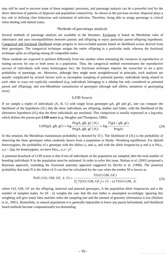
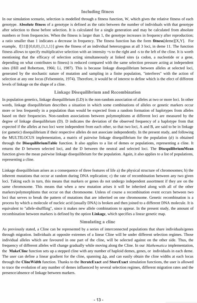
Variations in cline shape can be seen most easily by plotting allele frequency ratios on a logit scale,

Log p

q Log1 1

p 1. The logit function is the inverse of the "sigmoid", or "logistic" function commonly used in

mathematics (showed in Fig. 1). With the following command, we plot the cline maintained by stepped selection acrossan "ecotone" generated in the last section:


- 16 -


ListLogPlot1 1

AlleleFrequencyMeanres500 1 , Joined True, Axes True

5 10 15 20 25 30

0.1

1

10

100

Figure 5. LogPlot showing the cline shape with selection intensity s = 0.01 and migration mig = 0.5.

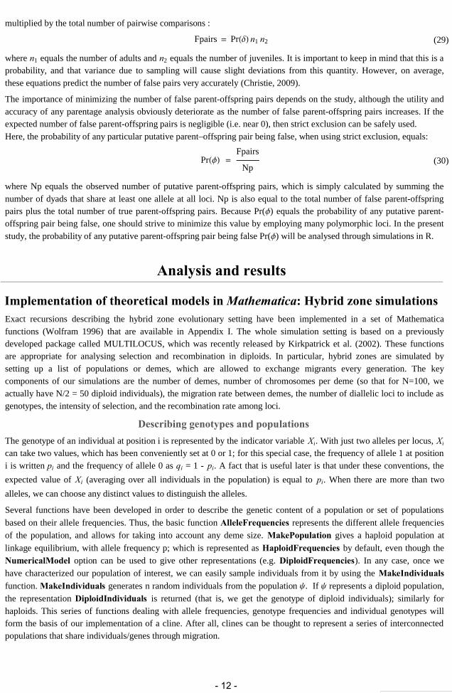
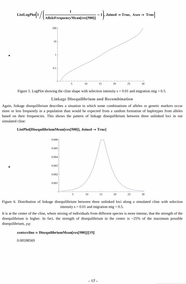
Linkage Disequilibrium and Recombination

Again, linkage disequilibrium describes a situation in which some combinations of alleles or genetic markers occurmore or less frequently in a population than would be expected from a random formation of haplotypes from allelesbased on their frequencies. This shows the pattern of linkage disequilibrium between three unlinked loci in oursimulated cline:

ListPlotDisequilibriumMeanres500, Joined True

5 10 15 20 25 30

0.001

0.002

0.003

0.004

0.005

0.006

Figure 6. Distribution of linkage disequilibrium between three unlinked loci along a simulated cline with selectionintensity s = 0.01 and migration mig = 0.5.

It is at the center of the cline, where mixing of individuals from different species is more intense, that the strength of thedisequilibrium is higher. In fact, the strength of disequilibrium in the centre is ~25% of the maximum possibledisequilibrium, pq:

centercline DisequilibriumMeanres500150.00598569


- 17 -


pp AlleleFrequencyMeanres50015;

maxdis DisequilibriumMeanres50015

pp1 pp0.0241168

centercline maxdis

0.248197

When loci are in the same chromosome, we say that they are linked. Only recombination can break down the jointsegregation of linked markers. In order to analyze the impact of recombination on the cline, we can set up simulationsfor different recombination levels r = {0.05, 0.1, 0.2, 0.5}:StoreExactres3, 0.04, , MakeCline30, 3, 100, fitness0.04, 15, ecotone, 0.5, 500, 20,

Linkage , , Compiled True,

FixedEnds MakePopulation3, 0, MakePopulation3, 1; & 0.05, 0.1, 0.2, 0.5;And now we show how the pattern of LD is reduced for increasing levels of recombination through a combined plot:

AllCline TableListPlotDisequilibriumMeanres3, 0.04, t500, Joined True,

PlotRange 0, 30, 0, 0.12, PlotStyle RGBColor12t^2, 2t^2, 20t^2, 0.9,t, 0.05, 0.1, 0.2, 0.5;ShowAllCline

Figure 7. Change on levels of linkage disequilibrium with different recombination rates: r = {0.05, 0.1, 0.2, 0.5}.

The value of D at the centre of the cline (deme number 15) for different levels of recombination will be:

DisequilibriumMeanres3, 0.04, 50015 & 0.05, 0.1, 0.2, 0.50.101872, 0.0641421, 0.0378334, 0.0194127 Simulating clines with different selection coefficients : Cline Width

In this case, results for a cline with selection intensity s = 0.08 are stored in res[3, 0.8][t]

StoreExactres3, 0.08, MakeCline30, 3, 100, fitness0.01, 15, ecotone, 0.5, 500, 20,Linkage 0.1, 0.1, Compiled True,

FixedEnds MakePopulation3, 0, 100, MakePopulation3, 1, 100;ListPlotDisequilibriumMeanres3, 0.08500, Joined True


- 18 -


5 10 15 20 25 30

0.005

0.010

0.015

0.020

Figure 8. Distribution of linkage disequilibrium between three loci along a simulated cline with selection intensity s =0.08.

It can be observed that the levels of Linkage Disequilibrium along the cline are more than 3 times higher thanpreviously obtained (Fig. 6)-We finally simulate the cline under different selection levels, ranging from 0.01 to 0.12:


Ifi mid, Times 1 sPlusXYLengthX, Times 1 sPlusXYLengthX;StoreExactres3, , ecotone, MakeCline30, 3, 100, fitness, 15, ecotone, 0.5, 500, 20,Compiled True, FixedEnds MakePopulation3, 0, MakePopulation3, 1; & 0.01, 0.02, 0.04, 0.08, 0.12;

It can be observed that with increasing selection pressure the cline gets steeper, so that the transition between one alleletype to the other is sharper.

AllCline TableListPlotAlleleFrequencyMeanres3, t, ecotone500, Joined True,

PlotRange 0, 30, 0, 1, PlotStyle RGBColor12t^2, 2t^2, 20t^2, 0.9,t, 0.01, 0.02, 0.04, 0.08, 0.12;ShowAllCline

Figure 9. Change on cline width at different selection levels.


- 19 -


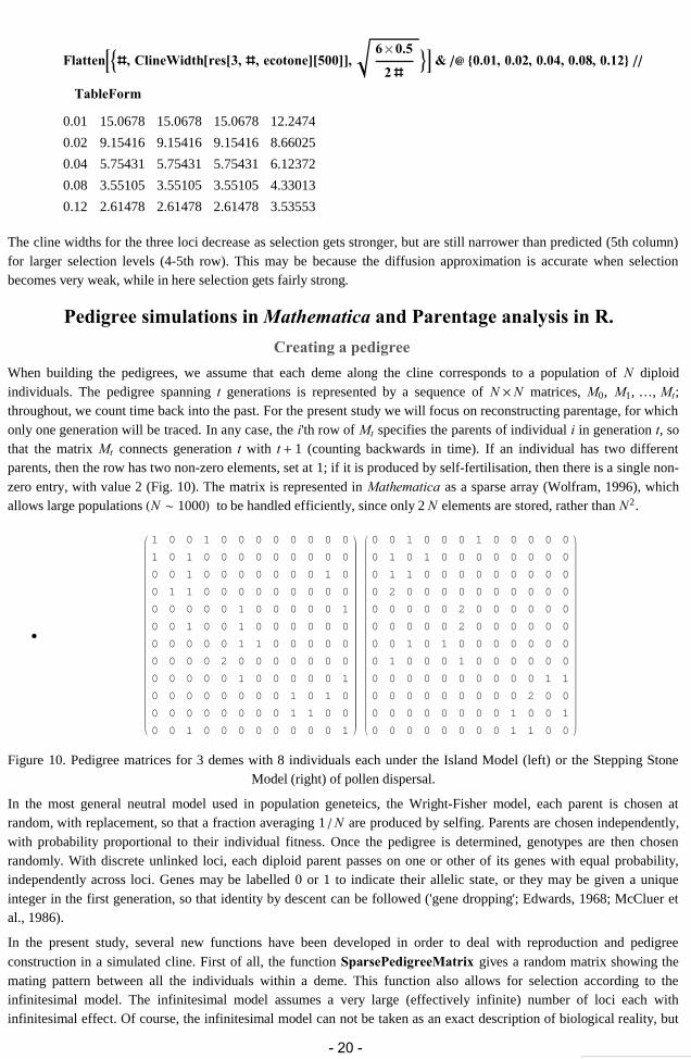
Flatten, ClineWidthres3, , ecotone500, 60.5

2 & 0.01, 0.02, 0.04, 0.08, 0.12

TableForm

0.01 15.0678 15.0678 15.0678 12.2474

0.02 9.15416 9.15416 9.15416 8.66025

0.04 5.75431 5.75431 5.75431 6.12372

0.08 3.55105 3.55105 3.55105 4.33013

0.12 2.61478 2.61478 2.61478 3.53553

The cline widths for the three loci decrease as selection gets stronger, but are still narrower than predicted (5th column)for larger selection levels (4-5th row). This may be because the diffusion approximation is accurate when selectionbecomes very weak, while in here selection gets fairly strong.

Pedigree simulations in Mathematica and Parentage analysis in R.

Creating a pedigree

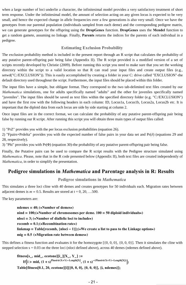
When building the pedigrees, we assume that each deme along the cline corresponds to a population of N diploidindividuals. The pedigree spanning t generations is represented by a sequence of N N matrices, M0, M1, …, Mt;throughout, we count time back into the past. For the present study we will focus on reconstructing parentage, for whichonly one generation will be traced. In any case, the i'th row of Mt specifies the parents of individual i in generation t, sothat the matrix Mt connects generation t with t 1 (counting backwards in time). If an individual has two differentparents, then the row has two non-zero elements, set at 1; if it is produced by self-fertilisation, then there is a single non-zero entry, with value 2 (Fig. 10). The matrix is represented in Mathematica as a sparse array (Wolfram, 1996), whichallows large populations N 1000 to be handled efficiently, since only 2N elements are stored, rather than N2.

1 0 0 1 0 0 0 0 0 0 0 0

1 0 1 0 0 0 0 0 0 0 0 0

0 0 1 0 0 0 0 0 0 0 1 0

0 1 1 0 0 0 0 0 0 0 0 0

0 0 0 0 0 1 0 0 0 0 0 1

0 0 1 0 0 1 0 0 0 0 0 0

0 0 0 0 0 1 1 0 0 0 0 0

0 0 0 0 2 0 0 0 0 0 0 0

0 0 0 0 0 1 0 0 0 0 0 1

0 0 0 0 0 0 0 0 1 0 1 0

0 0 0 0 0 0 0 0 1 1 0 0

0 0 1 0 0 0 0 0 0 0 0 1

0 0 1 0 0 0 1 0 0 0 0 0

0 1 0 1 0 0 0 0 0 0 0 0

0 1 1 0 0 0 0 0 0 0 0 0

0 2 0 0 0 0 0 0 0 0 0 0

0 0 0 0 0 2 0 0 0 0 0 0

0 0 0 0 0 2 0 0 0 0 0 0

0 0 1 0 1 0 0 0 0 0 0 0

0 1 0 0 0 1 0 0 0 0 0 0

0 0 0 0 0 0 0 0 0 0 1 1

0 0 0 0 0 0 0 0 0 2 0 0

0 0 0 0 0 0 0 0 1 0 0 1

0 0 0 0 0 0 0 0 1 1 0 0

Figure 10. Pedigree matrices for 3 demes with 8 individuals each under the Island Model (left) or the Stepping StoneModel (right) of pollen dispersal.

In the most general neutral model used in population geneteics, the Wright-Fisher model, each parent is chosen atrandom, with replacement, so that a fraction averaging 1 N are produced by selfing. Parents are chosen independently,with probability proportional to their individual fitness. Once the pedigree is determined, genotypes are then chosenrandomly. With discrete unlinked loci, each diploid parent passes on one or other of its genes with equal probability,independently across loci. Genes may be labelled 0 or 1 to indicate their allelic state, or they may be given a uniqueinteger in the first generation, so that identity by descent can be followed ('gene dropping'; Edwards, 1968; McCluer etal., 1986).

In the present study, several new functions have been developed in order to deal with reproduction and pedigreeconstruction in a simulated cline. First of all, the function SparsePedigreeMatrix gives a random matrix showing themating pattern between all the individuals within a deme. This function also allows for selection according to theinfinitesimal model. The infinitesimal model assumes a very large (effectively infinite) number of loci each withinfinitesimal effect. Of course, the infinitesimal model can not be taken as an exact description of biological reality, but


- 20 -


when a large number of loci underlie a character, the infinitesimal model provides a very satisfactory treatment of shortterm response. Under the infinitesimal model, the amount of selection acting on any given locus is expected to be verysmall, and hence the expected change in allele frequencies over a few generations is also very small. Once we have thegenotypes from our parental population (individuals sampled from each deme) and the corresponding pedigree matrix,

we can generate genotypes for the offspring using the DropGenes function. DropGenes uses the Mendel function toget a random gamete, assuming no linkage. Finally, Parents returns the indices for the parents of each individual in apedigree.

Estimating Exclusion Probability

The exclusion probability method is included in the present report through an R script that calculates the probability ofany putative parent-offspring pair being false (Appendix II). The R script provided is a modified version of a set ofscripts recently developed by Christie (2009). Before running this script you need to make sure that you set the workingdirectory within the script to a valid location so that R can read your input files and create output files (e.g.,setwd("C:/EXCLUSION")). This is easily accomplished by creating a folder in your C: drive called "EXCLUSION"-thedefault directory used throughout the script. Furthermore, the input files should be placed within this folder.

The input files have a simple, but obligate format. They correspond to the two tab-delimited text files created by ourMathematica simulations, one for adults specifically named "adults" and the other for juveniles specifically named"juveniles". The input files should be saved as text files within the specified directory folder (e.g. "C:/EXCLUSION")and have the first row with the following headers in each column: ID, Locus1a, Locus1b, Locus2a, Locus2b etc. It isimportant that the diploid data from each locus are side by side starting at column 2.

Once input files are in the correct format, we can calculate the probability of any putative parent-offspring pair beingfalse by running our R script. After running this script you will obtain three main types of output files called:

1) "PrZ" provides you with the per locus exclusion probabilities (equation 26).2) "Fpairs+Prdelta" provides you with the expected number of false pairs in your data set and Pr() (equations 29 and28, respectively).3) "Phi" provides you with Pr() (equation 30)-the probability of any putative parent-offspring pair being false.

Finally, the Putative pairs can be used to compare the R script results with the Pedigree structure simulated usingMathematica. Please, note that in the R code presented below (Appendix II), both text files are created independently ofMathematica, in order to simplify the presentation.

Pedigree simulations in Mathematica and Parentage analysis in R: Results

Pedigree simulations in Mathematica

This simulates a three loci cline with 40 demes and creates genotypes for 50 individuals each. Migration rates betweenadjacent demes is m 0.5. Results are stored at t = 0, 20, …500.

The key parameters are:

ndemes 40; Number of demesnind 100;Number of chromosomes per deme. 100 50 diploid individualsnloci 3; Number of diallelic loci to includerecomb 0.1;Recombination ratelinkmap Tablerecomb, nloci 1;We create a list to pass to the Linkage optionmig 0.5 Migration rate between demes

This defines a fitness function and evaluates it for the homozygote [{0, 0, 0}, {0, 0, 0}]. Then it simulates the cline withstepped selection s = 0.03 on the three loci (nloci defined above), across 40 demes (ndemes defined above).


Ifi mid, 1 sPlusXYLengthX, 1 sPlusXYLengthX;Tablefitness0.1, 20, ecotonei0, 0, 0, 0, 0, 0, i, ndemes;


- 21 -


StoreExactnew, MakeClinendemes, nloci, nind, fitness0.03, 20, ecotone, mig, 50, 2,Compiled True,

FixedEnds MakePopulationnloci, 0, ndemes, MakePopulationnloci, 1, ndemes; new50;

With this function we create a list containing the genotypes of 50 individuals from the whole cline sampled after 500generations. This will form our parental population.

popnews MakeIndividuals, Tablenind, ndemes;Now we can define the pedigree matrix for any specific deme within the cline. For example, this creates aPedigreeMatrix for 50 individuals and genotypes for 50 descendants from deme number 20.

pop1 popnews201;ped1 SparsePedigreeMatrixnind;off1 DropGenespop1, ped1;pop1 HaploidIndividualspop1;off1 HaploidIndividualsoff1;

This does the same but for the whole cline simultaneously. Note that we are calling Mendel directly without goingthrough DropGenes:

pop1 Tablepopnewsi1, i, ndemes;ped1 TableSparsePedigreeMatrixnind, ndemes;OffsCline TableMendelpop1i & Parentsped1i, i, ndemes;DimensionsOffsCline40, 100, 3

Effectively, we get alleles from 3 different markers in 40 demes with 100 haploid individuals (chromosomes) each.

pop11; OffsCline1; pop121; OffsCline21; pop140; OffsCline40;pop1 TableHaploidIndividualspop1i, i, ndemes;off1 TableHaploidIndividualsOffsClinei, i, ndemes;MakeDiploidpop123;MakeDiploidoff123;

Finally, we just need to Export our genotype table to a convenient text file, which will be used as input for the ExclusionProbability R scripts.


- 22 -


MakeDiploidpop1231;LengthFlattenMakeDiploidpop1231;TableFormPartitionFlattenMakeDiploidpop1231, nloci;Indlabels

FlattenTransposeTable"Ind"ToStringi, i, nind 2,Table"Ind"ToStringi, i, nind 2;

Pargenotypes

TableJoinFlatten"Individual", Table"Locus"ToStringi, i, nloci,FlattenTransposeIndlabels, PartitionFlattenMakeDiploidpop1j1, nloci,j, ndemes;

Filename Table"Parents" ToStringi ".txt", i, ndemes;DoExportToStringFilenamen, TableFormPartitionPargenotypesn, nloci 1,

"Table", n, ndemes;And we do the same for the Offspring genotypes.

MakeDiploidoff1231;LengthFlattenMakeDiploidoff1231;TableFormPartitionFlattenMakeDiploidoff1231, nloci;Indlabels

FlattenTransposeTable"Ind"ToStringi, i, nind 2,Table"Ind"ToStringi, i, nind 2;

Offgenotypes

TableJoinFlatten"Individual", Table"Locus"ToStringi, i, nloci,FlattenTransposeIndlabels, PartitionFlattenMakeDiploidoff1j1, nloci,j, ndemes;

Filename Table"Offspring" ToStringi ".txt", i, ndemes;DoExportToStringFilenamen, TableFormPartitionOffgenotypesn, nloci 1, "Table",n, ndemes;

Thus, we have a series of genotypes following the allele freuquencies imposed by the specific selection-gene flowpattern. Remember, we set up a cline with stepped selection s = 0.03 on three loci and with migration rates betweenadjacent demes mig 0.5.

Parentage analysis in R

Despite being able to simulate parent-offspring relationships within a simulated hybrid zone, the analysis of parentalexclusion was carried out in a simplified setting, given the limitations in time and computational resources. Thesimplified setting, which could be used as a minimum base-line for the efficiency of molecular markers, consists of asingle deme with allele frequencies following the Hardy-Weinberg equilibrium conditions.The number of loci used for this simulation study ranged from 10 to 20 molecular markers, which is within the standardnumber used in current paternity studies. Each molecular marker was allowed to be assigned a specific allele frequencydistribution, namely the Bernatchez, the Geometric or the Uniform distribution (Appendix II).

In the present study, neutral alleles were sampled from a geometric distribution, since this type of distribution iscommonly found in nature. The geometric distribution is the distribution of the total number of trials before the firstsuccess occurs, where the probability of success in each trial is p (Fig. 11).

ListPlotTablePDFGeometricDistribution0.3, k, k, 0, 30, PlotRange 0, 30, 0, 0.30,Filling Axis, Axes True


- 23 -


Figure 11. A geometric distribution with probability parameter p = 0.3.

This distribution of allele frequencies corresponds to the fact that only a few alleles are present in a significantproportion of individuals, while most alleles are only present in a few individuals.Our simulations allowed to define the index of individuals that produce offspring, which will be the ones that contributeto the next generation. These indices correspond to the pedigree matrices previously described. Finally, a proportion ofthe offspring population (False Offspring) is sampled from a new population, with a different allele frequencydistribution.

The calculation of Pr(Z) and Pr() as defined in equations (26) and (28) was carried out as indicated in the Methodssection. Only the alleles that are found both in the parentals and in the offspring were considered. It is important to notethat alleles occurring in only one sample (i.e. adults or juveniles) do not need to be included in the calculation becausetheir product equals zero.

Estimates of the probability of any putative parent–offspring pair being false (Phi; equation 30) were obtained throughthe R script included in Appendix II. Moreover, 10 replicates per parameter combination were carried out, in order toget a rough estimate of the variability found between different runs.

Figure 12. Estimated probability of any putative parent–offspring pair being false using a) 5 to 10 alleles in 10 to 16 locior b) 5 to 7 alleles in 10 to 20 loci.

The red line at 0.05 in figure 12 places the limit at which we would have 0.95 confidence in our parent-offspringassignments (= 0.05 False pairs). That is, it would mean we are accepting False parent-offspring pairs with lowprobability (which is what we want when doing parentage analysis). In the figure 12a, you can see 6 groups (5 to 10alleles) and 7 boxplots per group (10 to 16 loci). It is observed that if all markers had 5 alleles only (first group ofreplicates), we would need at least 15 markers to get 0.95 confidence in our parent-offspring assignments (= 0.05 False


- 24 -


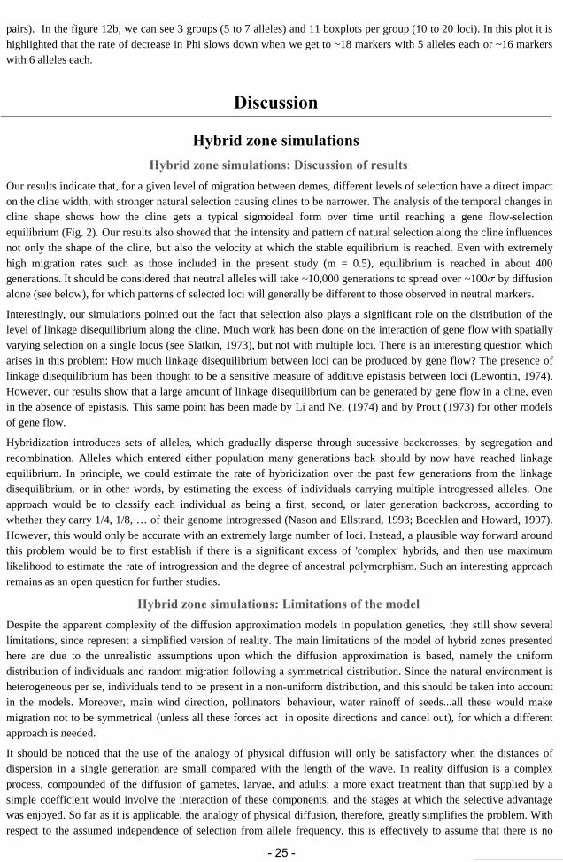
pairs). In the figure 12b, we can see 3 groups (5 to 7 alleles) and 11 boxplots per group (10 to 20 loci). In this plot it ishighlighted that the rate of decrease in Phi slows down when we get to ~18 markers with 5 alleles each or ~16 markerswith 6 alleles each.

Discussion

Hybrid zone simulations

Hybrid zone simulations: Discussion of results

Our results indicate that, for a given level of migration between demes, different levels of selection have a direct impacton the cline width, with stronger natural selection causing clines to be narrower. The analysis of the temporal changes incline shape shows how the cline gets a typical sigmoideal form over time until reaching a gene flow-selectionequilibrium (Fig. 2). Our results also showed that the intensity and pattern of natural selection along the cline influencesnot only the shape of the cline, but also the velocity at which the stable equilibrium is reached. Even with extremelyhigh migration rates such as those included in the present study (m = 0.5), equilibrium is reached in about 400generations. It should be considered that neutral alleles will take ~10,000 generations to spread over ~100 by diffusionalone (see below), for which patterns of selected loci will generally be different to those observed in neutral markers.

Interestingly, our simulations pointed out the fact that selection also plays a significant role on the distribution of thelevel of linkage disequilibrium along the cline. Much work has been done on the interaction of gene flow with spatiallyvarying selection on a single locus (see Slatkin, 1973), but not with multiple loci. There is an interesting question whicharises in this problem: How much linkage disequilibrium between loci can be produced by gene flow? The presence oflinkage disequilibrium has been thought to be a sensitive measure of additive epistasis between loci (Lewontin, 1974).However, our results show that a large amount of linkage disequilibrium can be generated by gene flow in a cline, evenin the absence of epistasis. This same point has been made by Li and Nei (1974) and by Prout (1973) for other modelsof gene flow.

Hybridization introduces sets of alleles, which gradually disperse through sucessive backcrosses, by segregation andrecombination. Alleles which entered either population many generations back should by now have reached linkageequilibrium. In principle, we could estimate the rate of hybridization over the past few generations from the linkagedisequilibrium, or in other words, by estimating the excess of individuals carrying multiple introgressed alleles. Oneapproach would be to classify each individual as being a first, second, or later generation backcross, according towhether they carry 1/4, 1/8, … of their genome introgressed (Nason and Ellstrand, 1993; Boecklen and Howard, 1997).However, this would only be accurate with an extremely large number of loci. Instead, a plausible way forward aroundthis problem would be to first establish if there is a significant excess of 'complex' hybrids, and then use maximumlikelihood to estimate the rate of introgression and the degree of ancestral polymorphism. Such an interesting approachremains as an open question for further studies.

Hybrid zone simulations: Limitations of the model

Despite the apparent complexity of the diffusion approximation models in population genetics, they still show severallimitations, since represent a simplified version of reality. The main limitations of the model of hybrid zones presentedhere are due to the unrealistic assumptions upon which the diffusion approximation is based, namely the uniformdistribution of individuals and random migration following a symmetrical distribution. Since the natural environment isheterogeneous per se, individuals tend to be present in a non-uniform distribution, and this should be taken into accountin the models. Moreover, main wind direction, pollinators' behaviour, water rainoff of seeds...all these would makemigration not to be symmetrical (unless all these forces act in oposite directions and cancel out), for which a differentapproach is needed.

It should be noticed that the use of the analogy of physical diffusion will only be satisfactory when the distances ofdispersion in a single generation are small compared with the length of the wave. In reality diffusion is a complexprocess, compounded of the diffusion of gametes, larvae, and adults; a more exact treatment than that supplied by asimple coefficient would involve the interaction of these components, and the stages at which the selective advantagewas enjoyed. So far as it is applicable, the analogy of physical diffusion, therefore, greatly simplifies the problem. Withrespect to the assumed independence of selection from allele frequency, this is effectively to assume that there is no


- 25 -


dominance in respect of the selective advantage enjoyed. Apart from its simplicity this is also the most important case toconsider, in respect to advantageous mutations occurring in nature. There are, at least, plausible reasons for supposingthat the common recessiveness of observed mutations is a characteristic of harmful mutations, which have long beenappearing in the species with relatively high mutation rates, whereas beneficial mutations must, at the time of theirestablishment, occur with exceedingly low mutation rates, and have rarely appeared before in the recent history of thespecies. On these grounds, dominance would be expected to be absent, and its absence is made more likely by the factthat in most cases the quantitative effect of beneficial mutations must be extremely small. For the same reason theselective intensity is taken to be a small quantity, so that the allele frequency (p) may be taken to vary continuously withtime, from generation to generation.

Although gene frequency can change abruptly across the centre of a hybrid zone, foreign alleles can still penetrate farinto either side. It is this gene flow between distinct populations that binds them together into one biological species.Smooth sigmoid clines are expected for introgressing alleles that are diffusing freely or are subject to only weakselection. A barrier to gene flow, caused for example by a physical obstacle, will produce a step in gene frequency, p,at the centre of the cline proportional to the gradient (dp/dx) on either side. The strength of this barrier to gene flow canbe estimated from the shape of the cline as B = p/(dp/dx).

Figure 13. Change in barrier strength depending on step 0 p 1 and gradient 0.001 p

x 0.01 in gene

frequency.

The barrier strength measure has the dimensions of distance (it can be considered as the equivalent unoccupied habitatthat would have a similar effect on gene flow reduction), and its magnitude relative to the dispersal rate (B/)determines the delay to the spread of genes across the barrier (Fig. 14). Although neutral alleles can suffer a lengthy

delay [T (B/2], alleles with even a slight advantage (s) will hardly be impeded (T log[(B/2s 2 2s). This is

because once a few of them penetrate the barrier, they will increase exponentially and spread to fixation. In makingthese comparisons it is important to note that even without barriers, neutral alleles will take ~10000 generations tospread over ~100 by diffusion alone (Barton, 1979).


- 26 -


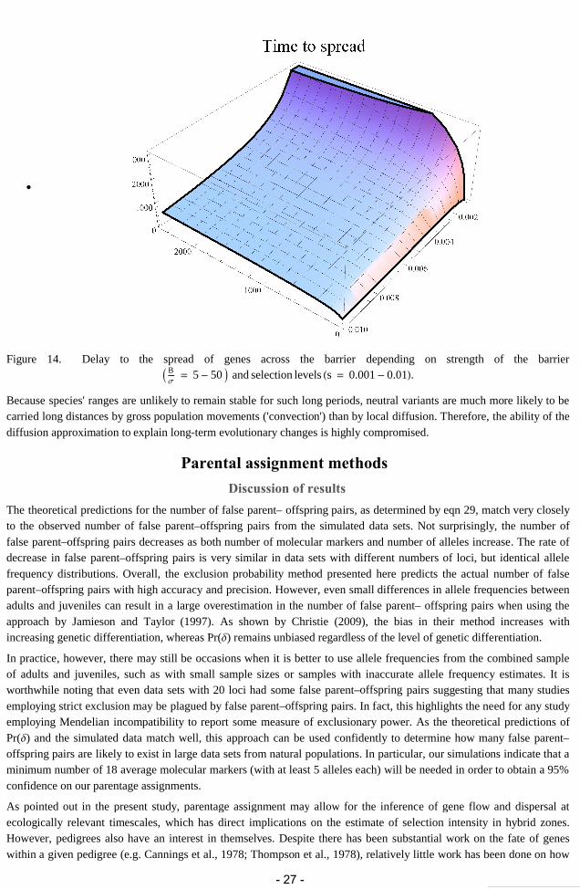
Figure 14. Delay to the spread of genes across the barrier depending on strength of the barrier B 5 50 and selection levels s 0.001 0.01.

Because species' ranges are unlikely to remain stable for such long periods, neutral variants are much more likely to becarried long distances by gross population movements ('convection') than by local diffusion. Therefore, the ability of thediffusion approximation to explain long-term evolutionary changes is highly compromised.

Parental assignment methods

Discussion of results

The theoretical predictions for the number of false parent– offspring pairs, as determined by eqn 29, match very closelyto the observed number of false parent–offspring pairs from the simulated data sets. Not surprisingly, the number offalse parent–offspring pairs decreases as both number of molecular markers and number of alleles increase. The rate ofdecrease in false parent–offspring pairs is very similar in data sets with different numbers of loci, but identical allelefrequency distributions. Overall, the exclusion probability method presented here predicts the actual number of falseparent–offspring pairs with high accuracy and precision. However, even small differences in allele frequencies betweenadults and juveniles can result in a large overestimation in the number of false parent– offspring pairs when using theapproach by Jamieson and Taylor (1997). As shown by Christie (2009), the bias in their method increases withincreasing genetic differentiation, whereas Pr() remains unbiased regardless of the level of genetic differentiation.

In practice, however, there may still be occasions when it is better to use allele frequencies from the combined sampleof adults and juveniles, such as with small sample sizes or samples with inaccurate allele frequency estimates. It isworthwhile noting that even data sets with 20 loci had some false parent–offspring pairs suggesting that many studiesemploying strict exclusion may be plagued by false parent–offspring pairs. In fact, this highlights the need for any studyemploying Mendelian incompatibility to report some measure of exclusionary power. As the theoretical predictions ofPr() and the simulated data match well, this approach can be used confidently to determine how many false parent–offspring pairs are likely to exist in large data sets from natural populations. In particular, our simulations indicate that aminimum number of 18 average molecular markers (with at least 5 alleles each) will be needed in order to obtain a 95%confidence on our parentage assignments.

As pointed out in the present study, parentage assignment may allow for the inference of gene flow and dispersal atecologically relevant timescales, which has direct implications on the estimate of selection intensity in hybrid zones.However, pedigrees also have an interest in themselves. Despite there has been substantial work on the fate of geneswithin a given pedigree (e.g. Cannings et al., 1978; Thompson et al., 1978), relatively little work has been done on how


- 27 -


pedigrees themselves evolve. From a genetic point of view, the pedigree constrains what genes can be passed on: withMendelian inheritance, selection acts solely through the different contributions made by individuals to the pedigree. Therecent availability of genomic sequences may focus more attention on pedigrees: given sufficient sequence data, wecould infer the pedigree many generations back; and given this pedigree, we could ask what contribution is likely to bemade to future generations by each ancestral genome. These questions are long-standing in evolutionary biology, but itwill become feasible to answer them only in the next few years.

Parentage Analysis: Limitations of the method

Exclusion is most powerful when there are few candidate parents and highly polymorphic genetic markers available.However, several caveats might be raised when the dataset at hand deviates from this ideal. Even high quality datasetscontain errors where at least one allele at a given locus does not match with what we expect from Mendelian laws. Thusit is unwise to exclude a parent immediately when observing such a mismatch. There are many reasons for suchmismatches, for example, genotyping errors. Genotyping errors occur when the genotype determined by molecularanalysis does not correspond to the real genotype. For instance, common genotyping errors in microsatellite datasets arenull alleles, which often result from a mutation in the primer annealing site. The most conservative way to handle alocus with null alleles in parentage analysis is to recode all homozygous genotypes as heterozygotes possessing thedetected allele and the null allele, thus preventing exclusion on the basis of homozygous genotypes.

Another potential weakness of a strict exclusion approach is that, if the ages of the sampled individuals are unknown,naïve application of parentage assignment methods can lead to problems where illegal pedigrees are proposed. Forexample, assigning parentage to a group of individuals from within the same group is likely to result in proposedpedigrees where an individual is its own grandparent. It should also be taken into account that, even though we are notconsidering extended families (multiple generations mixed together), nor variance in family size (some individualsproducing much more offspring than others), these factors would have a similar year-to-year effect than the highimmigration levels proposed in the present study, so they will not modify significantly our results. Moreover, despitesampling is done without replacement by default in R (in our simulations we are allowing each adult to produce onedescendant only), we could easily define different levels of variance in family size by using a specific probability vectorfor the offspring sampling process. Finally, it is worth noting that there have been few empirical studies comparing andvalidating the different approaches, despite the large variety of methodologies that currently exist for addressing manyof these problems (e.g. Butler et al., 2004; Csillery et al., 2006; Berger-Wolf et al., 2007).

Future studies: Analysing real data from Antirrhinum

Estimating selection from cline width and shape in a real setting

As indicated in the Introduction, the present study was originally motivated by a striking Antirrhinum hybrid zone(Whibley et al., 2006). Now we have a theoretical framework that will allow us to answer the questions proposed at thebeginning of this report. We can get estimates of natural selection while taking the effect of pollen dispersal (gene flow)into account. From previous studies we know that strong selection acts on several genes coding for the flower color suchas SULF, EL and ROS (Whibley et al., 2006). The widths of the clines at these loci, w, relative to the dispersal rate 2,

will give us a robust estimate of the strength of selection s acting to maintain them through the formula w ~ 2

2s.

Cline width will be determined directly from the genotyping data using EL, ROS and SULF markers. Note that we willhave estimates of dispersal from the parentage studies outlined above.

This is particularly relevant, since estimates of selection derived from cline width are robust because they do not dependstrongly on how selection acts, and because equilibrium is reached quickly. In addition, the detailed pattern of genotypefrequencies across the hybrid zone can tell us about the form of selection. For example, if alleles are recessive in theireffects on fitness, then they will introgress further (Mallet et al., 1990). Similarly, if one recombinant genotype is fitterthan other recombinants, then the clines will shift apart in its favour. This kind of asymmetry is what is predicted underDobzhansky-Muller models of speciation, and provides a route by which populations can diverge to becomeincompatible with each other, without passing through “adaptive valleys”. A good example is found in the burnet moth,Zygaena (Barton et al., 2007). A further issue that can be assessed is whether allele differences involve large shiftsalong an L-shaped path of high fitness (as in the classic Dobzhansky-Muller model) or whether it involves smaller steps


- 28 -


that take populations along a more diagonal path (Whibley et al., 2006), but those considerations fall well outside thescope of the present study.

Even though so far selection has only been observed for the three flower colour loci, it is possible that other loci are alsosubject to selection either via differences in pollination niche, or other components of fitness. In fact, hybrid zones thatare identified by one selected trait usually also prove to have other traits under selection (Barton and Hewitt, 1985), andone way of inferring selection at other loci is by measuring the barrier to gene flow at the zone of contact. It is worthnoting that, although the short scale estimates of gene flow and fitness through parentage analysis have the advantage ofbeing direct, they may be subject to environmental and population fluctuations from year to year, with temporalvariation in the magnitude of selection. If selection is less than a few percent such studies will be unable to detect it.Therefore, it is important to complement the above estimates with studies over the medium scale. Patterns of allelefrequency at neutral markers can tell us about the cumulative effects of gene flow across the whole genome. Thevariance in allele frequency over distance, FST, is widely used to estimate the relative rates of gene flow and randomdrift (Slatkin and Barton, 1990). Where populations are divided into discrete demes, FST allows the value of Nm to beestimated, where N is the deme size and m the number of migrants between demes per generation. Values of FST canbe obtained for the same marker loci used for paternity studies and from these estimates we could then infer dispersalrates m. These values could be then compared to those obtained from the short scale parentage studies. This type ofintegrative analysis of evolution at different temporal scales has never been carried out so far, and it will surely presentfurther challenges for the mathematical treatment of evolutionary processes.

AcknowledgementsThanks are due to all professors lecturing at MSc INVESTMAT both in Burjassot (Universitat de València) andTarongers (Universitat Politècnica de València), I really appreciate their effort in making mathematical conceptsaccessible to a biologist and their understanding with my insistence on bringing biology-related issues into focus whendiscussing every topic, from Algebra to Fuzzy Topology. Thanks are also due to prof. Guillermo Ayala, who kindlyaccepted to supervise this work. To all of them my best regards. This work was supported by a MSc fellowship awardedby LaCaixa Foundation to FP. This MSc thesis was carried out in order to fulfill the MSc INVESTMAT requirements.

ReferencesBarton, N.H. (1979). The dynamics of hybrid zones. Heredity 43: 341-359.

Barton, N.H. (1983). Multilocus clines. Evolution 37: 454-71.

Barton, N.H. and B.O. Bengtsson. (1986). The barrier to genetic exchange between hybridising populations. Heredity57: 357-376.

Barton, N.H. and K.S. Gale. (1993). Genetic analysis of hybrid zones. In: Hybrid zones and the evolutionary process(ed. R.G. Harrison), pp. 13-45. Oxford: Oxford University Press.

Barton, N.H. and G.M. Hewitt. (1985). Analysis of hybrid zones. Ann. Rev. Ecol. and Syst. 16: 113-148.

Barton, N H, and M. Turelli. (1991). Natural and sexual selection on many loci. Genetics 127: 229–255.

Barton, N.H., Briggs, D.E.G., Eisen, J.A., Goldstein, D.B. and N.H. Patel. (2007). Evolution. Cold Spring HarborLaboratory Press.

Bazykin, A.D. (1969). Hypothetical mechanism of speciation. Evolution 23: 685-731.

Bazykin, A.D. (1972). The disadvantage of heterozygotes in a population within a continuous area. Genetika 8: 162-67

Berger-Wolf, T.Y., Sheikh, S.I., DasGupta, B. et al. (2007). Reconstructing sibling relationships in wild populations.Bioinformatics 23: 49-56.

Boecklen, W.J. and D.J. Howard. (1997). Genetic analysis of hybrid zones: number of markers and power of resolution.Ecology 78: 2611-2616.

Butler, K., Field, C., Herbinger, C.M. and B.R. Smith. (2004). Accuracy, efficiency and robustness of four algorithms


- 29 -


allowing full-sib reconstruction from DNA marker data. Molecular Ecology 13: 1589-1600.

Capanna, E. (1980). Chromosomal rearrangement and speciation in progress in Mus musculus. Folia Zoologica 29:43-57.

Cannings, C., E. A. Thompson, and M. Skolnick. (1978). Probability functions on complex pedigrees. Advances inApplied Probability 10: 26-61.

Chakraborty, R., Meagher, T.R. and P.E. Smouse. (1988). Parentage analysis with genetic markers in naturalpopulations. I. The expected proportion of offspring with unambiguous paternity. Genetics 118: 527-536.

Christie, M. (2009). Parentage in natural populations: novel methods to detect parent-offspring pairs in large data sets.Molecular Ecology Resources doi: 10.1111/j.1755-0998.2009.02687.x

Csillery, K., Johnson, T., Beraldi, D. et al. (2006). Performance of marker based relatedness estimators in naturalpopulations of outbred vertebrates. Genetics 173: 2091-2101.

Derycke, S., Remerie, T., Backeljau, T. et al. (2008). Phylogeography of the Rhabditis (Pellioditis) marina speciescomplex: evidence for long-distance dispersal, and for range expansions and restricted gene flow in the northeastAtlantic. Molecular Ecology 17: 3306-3322.

Devlin, B. et al. (1988). Fractional paternity assignment: theoretical development and comparison to other methods.Theoretical and Applied Genetics 76: 369-380.

Dodds, K.G., Tate, M.L., McEwan, J.C., Crawford, A.M. (1996). Exclusion probabilities for pedigree testing farmanimals. Theoretical and Applied Genetics 92: 966-975.

Edwards, A.W.F. (1968). Simulation studies of genealogies. Heredity 23: 628.

Felsenstein, J. (1974). The evolutionary advantage of recombination. Genetics 78: 737-756.

Felsenstein, J. (1976). The theoretical population genetics of variable selection and migration. Ann. Rev. Genet. 10:253-80.

Fisher, R.A. (1930). The Genetical Theory of Natural Selection.Oxford: Oxford University Press.

Fisher, R.A. (1937). The wave of advance of advantageous genes. Ann. Eugenics 7: 355-369.

Garber, R.A. and J.W. Morris. (1983). General equations for the average power of exclusion for genetic systems of ncodominant alleles in one-parent and in no-parent cases of disputed parentage. In: Inclusion Probabilities in ParentageTesting (ed. R.H. Walker), pp. 277–280. American Association of Blood Banks, Arlington, VA.

Haldane, J.B.S. (1948). The theory of a cline. Journal of Genetics 48: 277-84.

Harrison, R.G. (1993). Hybrid zones and the evolutionary process. Oxford: Oxford University Press.

Hill, W.G. and A. Robertson. (1966). The effect of linkage on limits to artificial selection. Genetics Research 8:269-294.

Jamieson, A. and S.S. Taylor. (1997). Comparisons of three probability formulae for parentage exclusion. AnimalGenetics 28: 397-400.

Kauserud, H., Stensrud, O., Decock, C., Shalchian-Tabrizi, K. and T. Schumacher. (2006). Multiple gene genealogiesand AFLPs suggest cryptic speciation and long-distance dispersal in the basidiomycete Serpula himantioides(Boletales). Molecular Ecology 15: 421–431.

Kirkpatrick, M., Johnson, T. and N.H. Barton (2002). General models of multilocus evolution. Genetics 162: 1727-1750.

Jones, A.G. and W.R. Ardren. (2003). Methods of parentage analysis in natural populations. Molecular Ecology 12:2511-2523.

Lewontin, R.C. (1974). The genetic basis of evolutionary change. New York: Columbia University Press.

Li, W.H. and M. Nei. (1974). Stable linkage disequilibrium without epistasis in subdivided populations. TheoreticalPopulation Biology 6: 173-183.

Prout, T. (1973) Epistatis between functionally related isoenzymes of Mytilus edulis. Genetics 73: 493-496.

Manel, S., Gaggiotti, O.E. and R.S. Waples. (2005). Assignment methods: matching biological questions with


- 30 -


appropriate techniques. Trends in Ecology and Evolution 20: 136-142.

MacCluer, J.W., Vandeberg, J.L., Read, B. and O.A. Ryder. (1986). Pedigree analysis by computer simulation. ZoolBiol 5: 147-160.

Mallet J, Barton N, Lamas G, Santisteban J, Muedas M, Eeley H. (1990). Estimates of selection and gene flow frommeasures of cline width and linkage disequilibrium in Heliconius hybrid zones. Genetics 124: 921-936.

Milligan, B.G. (2003). Maximum-likelihood estimation of relatedness. Genetics 163: 1153-1167.

Moore, W.S. (1977). An evaluation of narrow hybrid zones in vertebrates. Q. Rev. Biol. 52: 263-78.

Nagylaki, T. (1975). Conditions for the existence of clines. Genetics 80, 595-615.

Nason, J. D. and N. C. Ellstrand. (1993). Estimating the frequencies of genetically distinct classes of individuals inhybridized populations. Journal of Heredity 84: 1-12.

Nathan R (2006). Long-distance dispersal of plants. Science, 313: 786–788.

Nielsen R, Mattila DK, Clapham PJ, Palsboll PJ (2001). Statistical approaches to paternity analysis in naturalpopulations and applications to the North Atlantic humpback whale. Genetics 157: 1673-1682.

Queller DC, Zacchi F, Cervo R et al. (2000). Unrelated helpers in a social insect. Nature. 405: 784–787.

Rouhani, S. and N. H. Barton. (1987). Speciation and the “shifting balance” in a continuous population. TheoreticalPopulation Biology 31: 465-492.

Slatkin, M. (1973). Gene flow and selection in a cline. Genetics 75: 733-56.

Slatkin, M. (1975). Gene flow and selection in a two-locus system. Genetics 81: 209-22.

Slatkin, M. and N.H. Barton. (1990). A comparison of three methods for estimating average levels of gene flow.Evolution 43: 1349-1368.

Thompson, E.A., C. Cannings and M.H. Skolnick. (1978). Ancestral inference I. The problem and the method. Annalsof Human Genetics 42: 95-108.

Turelli, M. and N.H. Barton. (1994). Genetic and statistical analyses of strong selection on polygenic traits: what, menormal? Genetics 138: 913-941.

Whibley, A.C., Langlade, N.B., Andalo, C., Hanna, A.I., Bangham, A., Thebaud, C. and E. Coen. (2006). Evolutionarypaths underlying flower color variation in Antirrhinum. Science 313: 963-966.

Wolfram, S. (1996). The Mathematica Book, 3rd edition. Wolfram Media, Cambridge Univ. Press, Cambridge.


- 31 -


APPENDIX I: CLINE SIMULATIONAND PEDIGREE FUNCTION

DEFINITION AlleleFrequencies

AlleleFrequencies::usage "AlleleFrequenciesp1,p2,…,n represents allele frequencies,and deme size n. AlleleFrequenciesp1,p2,… is shorthandfor AlleleFrequenciesp1,p2,…,1";

AlleleFrequenciesList : AlleleFrequencies, 1; AlleleFrequencyMean

AlleleFrequencyMean::usage "AlleleFrequencyMean gives the average frequency of 1alleles for the population representation . Also appliesto a list of 's, representing a cline. For representationsSymmetricNeutralHaploidFrequencies orSymmetricNeutralDiploidFrequencies, returns p,u, whereuis the average neutral allele frequency";

AlleleFrequencyMean : PopulationRepresentations, ...,optsRule : AlleleFrequencyMean, opts & ;

AlleleFrequencyMeanz : PopulationRepresentations, , optsRule :AlleleFrequencyTablez, opts .xList, y Meanx, y, xList Meanx;

AlleleFrequencyTable

AlleleFrequencyTable::usage "AlleleFrequencyTable gives the frequency of 1 alleles foreach locus. Also applies to a list of 's, representinga cline. For representations SymmetricNeutralHaploidFrequenciesor SymmetricNeutralDiploidFrequencies, returns p,p,…,u,where u

is the average neutral allele frequency.";


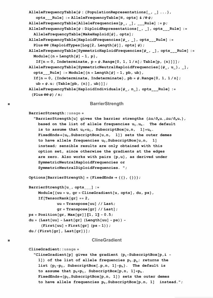
AlleleFrequencyTable : PopulationRepresentations, ...,optsRule : AlleleFrequencyTable, opts & ;

AlleleFrequencyTableAlleleFrequenciesp, , Rule : p;AlleleFrequencyTable : DiploidRepresentations, , optsRule :AlleleFrequencyTableMakeHaploid, opts;

AlleleFrequencyTableHaploidFrequencies, , optsRule :Plus HaploidTypesLog2, Length, opts;

AlleleFrequencyTableSymmetricHaploidFrequencies, , optsRule :Modulen Length 1, p,Ifn 0, Indeterminate, p .Range0, 1, 1 n; Tablep, n;

AlleleFrequencyTableSymmetricNeutralHaploidFrequencies, u, ,optsRule : Modulen Length 1, pb, ub,Ifn 0, Indeterminate, Indeterminate, pb .Range0, 1, 1 n;ub .u; Tablepb, n, ub;

AlleleFrequencyTableHaploidIndividuals, n, optsRule :Plus n; BarrierStrength

BarrierStrength::usage "BarrierStrengthu gives the barrier strengths uxu,uxu,based on the list of allele frequencies u1…un. The defaultis to assume that u0u1, SubscriptBoxu,n, 1un.FixedEndsu0,SubscriptBoxu,n, 1 sets the outer demesto have allele frequencies u0,SubscriptBoxu,n, 1instead; sensible results are only obtained with thisoption set, since otherwise the gradients at the edgesare zero. Also works with pairs p,u, as derived underSymmetricNeutralHaploidFrequencies orSymmetricNeutralDiploidFrequencies. ";

OptionsBarrierStrength FixedEnds , ;BarrierStrengthu, opts :

Moduleuu u, gr ClineGradientu, opts, du, ps,IfTensorRankgr 2,

uu Transposeuu Last;gr Transposegr Last;

ps Positiongr, Maxgr1, 1 0.5;du Lastuu LastgrLengthuu ps Firstuu Firstgrps 1;du Firstgr, Lastgr;

ClineGradient

ClineGradient::usage "ClineGradientp gives the gradient piSubscriptBoxp,i

1 of the list of allele frequencies p1…pn; returns thelist p1p0, SubscriptBox…p,n, 1pn. The default isto assume that p0p1, SubscriptBoxp,n, 1pn.FixedEndsp0,SubscriptBoxp,n, 1 sets the outer demesto have allele frequencies p0,SubscriptBoxp,n, 1 instead.";

2 MSc thesis - APPENDICES.nb


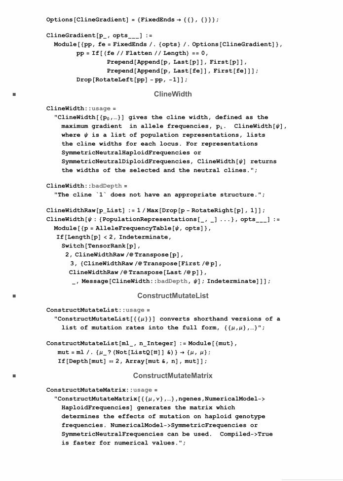
OptionsClineGradient FixedEnds , ;ClineGradientp, opts :

Modulepp, fe FixedEnds . opts . OptionsClineGradient,pp Iffe Flatten Length 0,

PrependAppendp, Lastp, Firstp,PrependAppendp, Lastfe, Firstfe;

DropRotateLeftpp pp, 1; ClineWidth

ClineWidth::usage "ClineWidthp0,… gives the cline width, defined as themaximum gradient in allele frequencies, pi. ClineWidth,where is a list of population representations, liststhe cline widths for each locus. For representationsSymmetricNeutralHaploidFrequencies orSymmetricNeutralDiploidFrequencies, ClineWidth returnsthe widths of the selected and the neutral clines.";

ClineWidth::badDepth "The cline `1` does not have an appropriate structure.";

ClineWidthRawpList : 1 MaxDropp RotateRightp, 1;ClineWidth : PopulationRepresentations, ..., opts :

Modulep AlleleFrequencyTable, opts,IfLengthp 2, Indeterminate,SwitchTensorRankp,2, ClineWidthRaw Transposep,3, ClineWidthRaw TransposeFirst p,ClineWidthRaw TransposeLast p,, MessageClineWidth::badDepth, ; Indeterminate;

ConstructMutateList

ConstructMutateList::usage "ConstructMutateList converts shorthand versions of alist of mutation rates into the full form, ,,…";

ConstructMutateListml, nInteger : Modulemut,mut ml . ?NotListQ & , ;IfDepthmut 2, Arraymut &, n, mut;

ConstructMutateMatrix

ConstructMutateMatrix::usage "ConstructMutateMatrix,,…,ngenes,NumericalModelHaploidFrequencies generates the matrix whichdetermines the effects of mutation on haploid genotypefrequencies. NumericalModelSymmetricFrequencies orSymmetricNeutralFrequencies can be used. CompiledTrueis faster for numerical values.";

MSc thesis - APPENDICES.nb 3


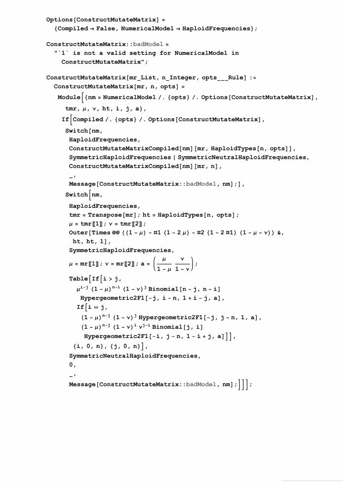
OptionsConstructMutateMatrix Compiled False, NumericalModel HaploidFrequencies;ConstructMutateMatrix::badModel "`1` is not a valid setting for NumericalModel inConstructMutateMatrix";

ConstructMutateMatrixmrList, nInteger, optsRule :ConstructMutateMatrixmr, n, opts Modulenm NumericalModel . opts . OptionsConstructMutateMatrix,tmr, , , ht, i, j, a,IfCompiled . opts . OptionsConstructMutateMatrix,Switchnm,HaploidFrequencies,ConstructMutateMatrixCompilednmmr, HaploidTypesn, opts,SymmetricHaploidFrequencies SymmetricNeutralHaploidFrequencies,ConstructMutateMatrixCompilednmmr, n,,

MessageConstructMutateMatrix::badModel, nm;,Switchnm,HaploidFrequencies,tmr Transposemr; ht HaploidTypesn, opts; tmr1; tmr2;OuterTimes 1 11 2 21 211 &,ht, ht, 1,SymmetricHaploidFrequencies,

mr1; mr2; a

1

1 ;

TableIfi j,ij1 ni1 jBinomialn j, n iHypergeometric2F1j, i n, 1 i j, a,

Ifi j,1 nj1 j Hypergeometric2F1j, j n, 1, a,1 nj1 ijiBinomialj, iHypergeometric2F1i, j n, 1 i j, a,i, 0, n, j, 0, n,

SymmetricNeutralHaploidFrequencies,0,,

MessageConstructMutateMatrix::badModel, nm;;



ConstructMutateMatrixCompiled

ConstructMutateMatrixCompiled::usage "ConstructMutateMatrixCompiledHaploidFrequencies,,…,0,…,…

gives the mutation matrix; called byConstructMutateMatrix…,CompiledTrue.ConstructMutateMatrixCompiledSymmetricHaploidFrequencies,,ngenes is also defined, as isConstructMutateMatrixCompiledSymmetricHaploidFrequencies,,ngenes.";

ConstructMutateMatrixCompiledHaploidFrequencies Compilemr, Real, 2, ht, Integer, 2,Moduletmr Transposemr, j, k,TableTimes 1 tmr1 htj1 2tmr1

htk1 2htj1 tmr1 tmr2, j, Lengthht,k, Lengthht,tmr, Real, 2, j, Integer, k, Integer;ConstructMutateMatrixCompiledSymmetricHaploidFrequencies Compilemr, Real, 1, n, Integer,Modulei, j, a, , , mr1; mr2; a

1

1 ;

TableIfi j,ij1 ni1 jBinomialn j, n iHypergeometric2F1j, i n, 1 i j, a,

Ifj i,1 nj1 j Hypergeometric2F1j, j n, 1, a,Binomialj, i1 nj1 ijiHypergeometric2F1i, j n, 1 i j, a,i, 0, n, j, 0, n,a, Real, , Real, , Real, i, Integer, j, Integer,Binomial, , Real;

DemeSize

DemeSize::usage "DemeSize gives the deme size associated with the populationrepresentation ; also applies to a cline.";

DemeSizePopulationRepresentations, n : n;DemeSize : PopulationRepresentations, ... : DemeSize ;



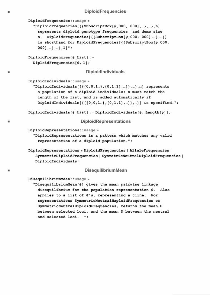
DiploidFrequencies

DiploidFrequencies::usage "DiploidFrequenciesSubscriptBox,000, 000,…,…,nrepresents diploid genotype frequencies, and deme sizen. DiploidFrequenciesSubscriptBox,000, 000,…,…is shorthand for DiploidFrequenciesSubscriptBox,000,000,…,…,1";

DiploidFrequenciesList :DiploidFrequencies, 1;

DiploidIndividuals

DiploidIndividuals::usage "DiploidIndividuals0,0,1…,0,1,1,…,…,n representsa population of n diploid individuals; n must match thelength of the list, and is added automatically ifDiploidIndividuals0,0,1…,0,1,1,…,… is specified.";

DiploidIndividualsList : DiploidIndividuals, Length; DiploidRepresentations

DiploidRepresentations::usage "DiploidRepresentations is a pattern which matches any validrepresentation of a diploid population.";

DiploidRepresentations DiploidFrequencies AlleleFrequencies SymmetricDiploidFrequencies SymmetricNeutralDiploidFrequencies DiploidIndividuals;

DisequilibriumMean

DisequilibriumMean::usage "DisequilibriumMean gives the mean pairwise linkagedisequilibrium for the population representation . Alsoapplies to a list of 's, representing a cline. Forrepresentations SymmetricNeutralHaploidFrequencies orSymmetricNeutralDiploidFrequencies, returns the mean Dbetween selected loci, and the mean D between the neutraland selected loci. ";



DisequilibriumMean : PopulationRepresentations, ...,optsRule :DisequilibriumMean, opts & ;

DisequilibriumMeanpr : NonNeutralRepresentations, , optsRule :Modulen, dt DisequilibriumTablepr, opts,n Lengthdt;Plus Plus Array1 &, n, n IdentityMatrixndt 1

nn 1;DisequilibriumMeanpr : NeutralRepresentations, , optsRule :Modulen, dt DisequilibriumTablepr, opts,n Lengthdt1;Plus Plus Array1 &, n, n IdentityMatrixndt1 1

nn 1,Meandt2;

DisequilibriumTable

DisequilibriumTable::usage "DisequilibriumTable gives a matrix of pairwise linkagedisequilibrium for the population representation . Alsoapplies to a list of 's, representing a cline. Forrepresentations SymmetricNeutralHaploidFrequencies orSymmetricNeutralDiploidFrequencies, returns the D betweenselected loci, and the D between the neutral and selectedloci. DisequilibriumMean gives the mean pairwise linkagedisequilibrium for the population representation . Alsoapplies to a list of 's, representing a cline. Forrepresentations SymmetricNeutralHaploidFrequencies orSymmetricNeutralDiploidFrequencies, returns the mean Dbetween selected loci, and the mean D between the neutraland selected loci. ";



DisequilibriumTable : PopulationRepresentations, ...,optsRule :DisequilibriumTable, opts & ;

DisequilibriumTableAlleleFrequenciesp, , Rule :DiagonalMatrixp1 p;

DisequilibriumTable : DiploidRepresentations, , optsRule :DisequilibriumTableMakeHaploid, opts;

DisequilibriumTableHaploidFrequencies, , optsRule :Modulen Log2, Length,p AlleleFrequencyTableHaploidFrequencies, opts, dk,dk p & HaploidTypesn, opts;.OuterTimes, , & dk;

DisequilibriumTableSymmetricHaploidFrequencies, nd,optsRule :Modulen Length 1,p AlleleFrequencyMeanSymmetricHaploidFrequencies, nd, opts,d, du,d

.Range0, n n p2 n p1 pnn 1 ;

IdentityMatrixnp1 p d Arrayd &, n, n;DisequilibriumTableSymmetricNeutralHaploidFrequencies, u, nd,

optsRule :Modulen Length 1,pu AlleleFrequencyTableSymmetricNeutralHaploidFrequencies, u, nd, opts, p, ub, d, du,p pu1, 1; ub pu2;d

n .Range0, 1, 1n p2 p1 pn 1 ;

du Range0, 1,1

n p .u ub;IdentityMatrixnp1 p d Arrayd &, n, n,

Arraydu &, n;DisequilibriumTableHaploidIndividuals, nd, optsRule :

Modulenl Length1,p AlleleFrequencyTableHaploidIndividuals, nd,Ifnd 2, ArrayIndeterminate &, nl, nl,Plus OuterTimes, p, p & nd 1;



DoubleCline

DoubleCline::usage "DoubleCline,EvenQndemes takes the cline to representthe left half of a symmetric cline, and adds the righthalf. If the total number of demes is even, then thesecond argument is set True, and the extra demes are amirror image of . If the total number of demes is odd,the second argument is set False, and Last is assumedto be the central deme; it must contain a symmetrical setof genotype frequencies. ";

DoubleCline : IndividualRepresentations AlleleFrequencies, ...,eQ :Join,ReverseIfeQ, , Drop, 1 .pr : PopulationRepresentationsf, n : pr1 f, n;

DoubleCline :HaploidFrequencies DiploidFrequencies

SymmetricHaploidFrequencies SymmetricDiploidFrequencies, ..., eQ :

Join,ReverseIfeQ, , Drop, 1 .pr : PopulationRepresentationsf, n : prReversef, n;

DoubleCline : NeutralRepresentations, ..., eQ :Join,ReverseIfeQ, , Drop, 1 .pr : NeutralRepresentationsf, u, n :

prReversef, 1 Reverseu, n; DropGenes

DropGenes::usage "DropGenesp,P generates random genotypes, given the pedigreeP; uses Mendel. Mendel0,1,…,1,0,… gives a randomgamete, assuming no linkage. DropGenesp0,P1,… doesthe same for many generations";

DropGenesp : ..., PSparseArray : Mendelp & ParentsP;DropGenesp : ..., PSparseArray : Mendelp & ParentsP;DropGenesp0 : ..., Pl : SparseArray :FoldListDropGenes, p0, Pl;



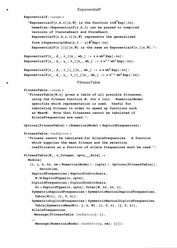
ExponentialF

ExponentialF::usage

"ExponentialFr,,n,W is the function rnWExpn.

DemeSizeExponentialFr,, can be passed to compiledversions of IterateExact and StoreExact.

ExponentialFr,,,n,W represents the generalised

form rSuperscriptBoxn,1 WExpn.ExponentialFr…jn,W is the same as ExponentialFr…n,W.";

ExponentialFr, , n, wb : rnwbExpn;ExponentialFr, , , n, wb : rn1wbExpn;ExponentialFr, , n, wb : rnwbExpn;ExponentialFr, , , n, wb : rn1wbExpn;

FitnessTable

FitnessTable::usage "FitnessTableW,n gives a table of all possible fitnesses,using the fitness function W, for n loci. NumericalModelspecifies which representation is used. Useful fortabulating fitness in order to speed up functions suchas MeanW. Note that fitnesses cannot be tabulated ifAlleleFrequencies are used.";

OptionsFitnessTable NumericalModel HaploidFrequencies;FitnessTable::badOption "Fitness cannot be tabulated for AlleleFrequencies. A functionwhich supplies the mean fitness and the selectioncoefficients as a function of allele frequencies must be used.";

FitnessTableW, nInteger, optsRule :Modulei, j, h, ht, nm NumericalModel . opts . OptionsFitnessTable,

Switchnm,HaploidFrequencies HaploidIndividuals,W HaploidTypesn, opts,

DiploidFrequencies DiploidIndividuals,ht HaploidTypesn, opts; OuterW, ht, ht, 1,

SymmetricHaploidFrequencies SymmetricNeutralHaploidFrequencies,TableWi, i, 0, n,

SymmetricDiploidFrequencies SymmetricNeutralDiploidFrequencies,TableSymmetricMeanWi, j, n, W, i, 0, n, j, 0, n,

AlleleFrequencies,MessageFitnessTable::badOption; ,

,

MessageNumericalModel::badSetting, nm; ;



FixedEnds

FixedEnds::usage "FixedEnds is an option for MigrateExact and related functionswhich specifies that endpoints should be fixed. FixedEndsspecifies a source population that provides migrants intoa single deme. FixedEnds0,1 fixes genotype frequenciesat 0, 1 at either end of a cline.";

FrequencyRepresentations

FrequencyRepresentations::usage "FrequencyRepresentations is a pattern which matches any validrepresentation of a population by allele, class or genotypefrequencies.";

FrequencyRepresentations HaploidFrequencies DiploidFrequencies AlleleFrequencies SymmetricHaploidFrequencies SymmetricDiploidFrequencies SymmetricNeutralHaploidFrequencies SymmetricNeutralDiploidFrequencies;

Gametes

Gametes::usage "GametesY,Z gives the full distribution of 2noffspringgenotypes. LligamSubscriptBox\r\,\1,\\\\\\\\\\\\ \\\\\\\\\ \\\\\ \\\\\\\\\\\ \\\\\\\ \\\\ \\\\\\\ \\\\\2\\\\\,SubscriptBox\r\,\2,\\\\\ \\\\\\\\\\\\\\\\ \\\3\\\\,… specifies a lineargenetic map. GametesX,Y,Z is also defined, and givesthe probability of a specific gamete X from diploid parentY,Z. Gametesi,j,n,NumericalModelSymmetricHaploidFrequenciesgives the distribution of genotypes among gametes from aparent of genotype i,j.Gametesi,j,n,W,NumericalModelSymmetricHaploidFrequenciesgives the same, for fitness Wi,j,h. NOT normalised byMeanW, however.";

OptionsGametes Lligam False;GametesiInteger, jInteger, nInteger : Gametesi, j, n, 1 &;GametesYList, ZList, optsRule : GametesY, Z, 1 &, opts;GametesiInteger, jInteger, nInteger, W :

Modulel, k,2ij

Binomialn, j Sum22lTableBinomiali j 2l, k l, k, 0, nBinomiali, lBinomialn i, j lWi, j, i j 2l,l, Max0, i j n, Mini, j;



GametesYList, ZList, W, optsRule :GametesRaw, Y, Z, opts & HaploidTypesLengthZ, optsWY, Z;GametesRawXList, YList, ZList, optsRule :

Moduleph, rr, rQ,r Lligam . opts . OptionsGametes,h Y Z 2Y Z,p 1 X Y 2X Y,

ph FlattenPositionh, 1;IfTimes h 1 hp 0,

0,Ifr False ph ,Times 1 h 2,

rr PrependNetRecombination Taker, & DropTransposeph, RotateLeftph 1, 1,1 2;

rQ p & ph;rQ AbsrQ RotateRightrQ;

Times 1 rr rQ2rr 1; GameteTable

GameteTable::usage "GameteTablen gives the full distribution of 2n offspringgenotypes. LligamSubscriptBox\r\,\1,\\\\\\\\\\\\ \\\\\\\\\ \\\\\\\\\\\\2\\\\,SubscriptBox\r\,\2,\\\\\\\\\\\\ \\\\\\\\\ \\\\\\\\\\\\3\\\\,… specifies a linear genetic map.GameteTablen,NumericalModelSymmetricHaploidFrequenciesstores a matrix showing the distribution of genotypesamong gametes, for each diploid genotype, under thesymmetric model. GameteTablen,W is also defined; itallows for a fitness function W. Results are stored,which greatly speeds calculations. However, if fitnessescontinually change, the option StoreResultsFalse must be used.";

OptionsGameteTable Lligam False, StoreResults True,NumericalModel HaploidFrequencies;

GameteTable::badOpts "`1` is not a valid option for GameteTable";

GameteTablenInteger, optsRule : GameteTablen, 1 &, opts;



GameteTablenInteger, ww, optsRule :Modulei, j, ht,nm NumericalModel . opts . OptionsGameteTable,srQ StoreResults . opts . OptionsGameteTable,IfsrQ,

GameteTablen, ww, opts GameteTablen, ww, StoreResults False, opts,Switchnm,SymmetricRepresentations,TableGametesi, j, n, ww, i, 0, n, j, 0, n,NonSymmetricRepresentations,ht HaploidTypesn, opts;

OuterGametes1, 2, ww, opts &, ht, ht, 1,,MessageGameteTable::badOpts, nm;

HaploidFrequencies

HaploidFrequencies::usage "HaploidFrequencies000,…,n represents haploid genotypefrequencies, and deme size n. HaploidFrequencies000,…is shorthand for HaploidFrequencies000,…,1";

HaploidFrequenciesList :HaploidFrequencies, 1;

HaploidIndividuals

HaploidIndividuals::usage "HaploidIndividuals0,0,1…,…,n represents a populationof n haploid individuals; n must match the length of thelist, and is added automatically ifHaploidIndividuals0,0,1…,… is specified.";

HaploidIndividualsList : HaploidIndividuals, Length; HaploidRepresentations

HaploidRepresentations::usage "HaploidRepresentations is a pattern which matches any validrepresentation of a haploid population.";

HaploidRepresentations HaploidFrequencies AlleleFrequencies SymmetricHaploidFrequencies SymmetricNeutralHaploidFrequencies HaploidIndividuals;



HaploidTypes[{{a1,b1,..},{a2,b2,..}..}] lists all possible haploid genotypes, based on theset of alleles {a1,b1,..} at locus 1, etc. HaploidTypes[{{a,b,..},n}] lists all possible

genotypes, assuming the same set of alleles at n loci. HaploidTypes[n] assumes nloci, with two alleles labelled {0,1}. HaploidTypes[n,SortByClassTrue] lists

haplotypes ordered by the # of '1' alleles.

HaploidTypes::usage "HaploidTypesa1,b1,..,a2,b2,.... lists all possiblehaploid genotypes, based on the set of alleles a1,b1,..at locus 1, etc. HaploidTypesa,b,..,n lists allpossible genotypes, assuming the same set of alleles atn loci. HaploidTypesn assumes n loci, with two alleleslabelled 0,1. HaploidTypesn,SortByClassTrue listshaplotypes ordered by the of '1' alleles.";

OptionsHaploidTypes SortByClass False;HaploidTypes, : ;HaploidTypesgList, opts :HaploidTypesg, opts IfSortByClass . opts . OptionsHaploidTypes,

SortHaploidTypesg,Modulep1 Plus 1, p2 Plus 2,Ifp1 p2, True, Ifp1 p2, False, OrderedQ1, 2 &,

FlattenApplyOuter, Prependg, List, Lengthg 1;HaploidTypesgList, nInteger, opts :HaploidTypesg, n, opts HaploidTypesTableg, n, opts;

HaploidTypesnInteger, opts :HaploidTypesn, opts HaploidTypes0, 1, n, opts;

HeterozygoteB

HeterozygoteB::usage "HeterozygoteBi,j,n gives the distribution of the ofheterozygous loci among gametes from a parent of genotypei,j, under the symmetric model. HeterozygoteBn storesa table of HeterozygoteBi,j,n for i0…n, j0…n.";

HeterozygoteBi, j, n : HeterozygoteBi, j, n Modulel, pp Array0 &, n 1,

Doppi j 2l 1 Binomiali, lBinomialn i, j l ,l, Max0, i j n, Mini, j; pp Binomialn, j;HeterozygoteBn : HeterozygoteBn

Modulei, j, TableHeterozygoteBi, j, n, i, 0, n,j, 0, n;



IndividualRepresentations

IndividualRepresentations::usage "IndividualRepresentations is a pattern which matches anyvalid representation of a population as a list of individuals.";

IndividualRepresentations HaploidIndividuals DiploidIndividuals; IterateExact

IterateExact::usage "IterateExact,W,0 gives gamete frequencies after onegeneration of selection; may represent a single deme,or an array of demes, but must represent a haploidpopulation. IterateExact,W,m allows for migration.If contains only a single population, then it iteratesthat deme, with immigration from a source of the samesize, fixed for 1,1…; FixedEndss specifies anarbitrary source population. The fitness is representedby a function Wi,j,h in the symmetrical model, WX,Yif all 2n genotypes are iterated, or WpW,s1,… ifonly AlleleFrequencies are supplied. If consists of alist of demes, migration is at a rate m2 to each neighbour.The fitness is then represented by a function Wdemei,j,hin the symmetrical model, or WdemeX,Y if all 2n

genotypes are iterated. CompiledTrue uses compiled code.The default order is random unionmigrationselectionmeiosis,which is represented by MigrationOrderUMS. MigrationOrderMUSrepresents migrationrandom unionselectionmeiosis.MigrationOrderUSM represents randomunionselectionmigrationmeiosis. For a cline,FixedEnds0,1 fixes genotype frequencies at 0, 1at either end. For SymmetricNeutralHaploidFrequencies,IterateExact,u,W,m,u includes the frequency ofthe neutral marker after one generation of selectionfollowed by immigration from a source population withfrequency u. DemeSizeF allows deme size to change to

some function Fn,W, where n is the number beforeselection. Compiled code can only use a limited set ofF: either n&, where n is a fixed number; or ExponentialFr,,,which represents rnW

Expn; or PowerFr,,, which

represents rSuperscriptBoxn,1 W. RandomDriftTrue

includes random sampling of a number of haploid gametesequal to the deme size after selection.";

OptionsIterateExact Compiled False, MigrationOrder UMS,FixedEnds , , DemeSize 1 &, RandomDrift False;

IterateExact::badMigrationOrder "`1` is not a valid setting for MigrationOrder";



IterateExact one deme

IterateExactpr : NonNeutralRepresentations, nd, ww, m,optsRule : Modulei, gg, s, f, cr, gt, dt, ht,iQ MatchQpr, HaploidIndividuals,cQ Compiled . opts . OptionsIterateExact,mo MigrationOrder . opts . OptionsIterateExact,fe FixedEnds . opts . OptionsIterateExact,rd RandomDrift . opts . OptionsIterateExact,ng NumberOfGenespr, nd, spr,s Iffe1 fe1 ,spr Switchpr,HaploidIndividuals, HaploidFrequencies,, pr;

MakePopulationng, 1, nd, NumericalModel spr,fe1;

IfcQ,f DemeSize . opts . OptionsIterateExact;f f . nn?NumberQ & nn, 0, 1, 0, 1 & 1, 0, 0, 0,

PowerFr, , r, , , 0,ExponentialFr, , r, , 0, ,PowerF ExponentialFr, , , r, , , ,ExponentialFr, , r, , 0, ;

cr Ifpr AlleleFrequencies,IterateCompiledww, oneDeme, mo, nd, m, s1, s2, f, rd,gt GameteTableng, ww, NumericalModel pr, opts;IfiQ,ht HaploidTypesLog2, Lengths1, opts;FlattenOuterList, ht, ht, 1, 1;IterateCompiledoneDeme, ind, mo, nd, gt, dt, m, s1, s2, f,IterateCompiledoneDeme, mo, nd, gt, m, s1, s2, f, rd;

prDropcr, 1, Lastcr,Switchmo,UMS,NewGametesMigrateExactMakeDiploidpr, nd, MakeDiploids, m,ww, opts,MUS,NewGametesMakeDiploidMigrateExactpr, nd, s, m, ww, opts,USM,2 IfiQ OddQnd, MakeDiploidprDrop, 1, nd 1,

MakeDiploidpr, nd;MigrateExactNewGametes2, ww, opts, s, m,, MessageIterateExact::badMigrationOrder, mo; pr, nd;



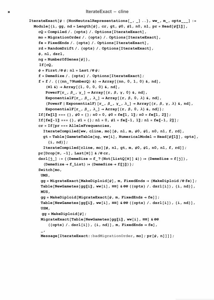
IterateExact cline

IterateExact : NonNeutralRepresentations, .., ww, m, opts :Modulei, gg, nd Length, cr, gt, 0, 1, n0, n1, pr Head1,cQ Compiled . opts . OptionsIterateExact,mo MigrationOrder . opts . OptionsIterateExact,fe FixedEnds . opts . OptionsIterateExact,rd RandomDrift . opts . OptionsIterateExact,, nl, dsrl,ng NumberOfGenes,IfcQ, First ; nl Last ;f DemeSize . opts . OptionsIterateExact;f f . nn?NumberQ & Arraynn, 0, 1, 0 &, nd,1 & Array1, 0, 0, 0 &, nd,

PowerFr, , Arrayr, , , 0 &, nd,ExponentialFr, , Arrayr, , 0, &, nd,PowerF ExponentialFr, , , Arrayr, , , &, nd,ExponentialFr, , Arrayr, , 0, &, nd;

Iffe1 , 0 ; n0 0, 0 fe1, 1; n0 fe1, 2;Iffe1 , 1 ; n1 0, 1 fe1, 1; n1 fe1, 2;cr Ifpr AlleleFrequencies,IterateCompiledww, cline, mo, nl, m, 0, 1, n0, n1, f, rd,gt TableGameteTableng, wwi, NumericalModel Head1, opts,i, nd;IterateCompiledcline, mo, nl, gt, m, 0, 1, n0, n1, f, rd;

prDrop, 1, Last & cr,dsrlj : DemeSize f?NotListQ & DemeSize fj,DemeSize fList DemeSize fj;Switchmo,UMS,gg MigrateExactMakeDiploid, m, FixedEnds MakeDiploid fe;TableNewGametesggi, wwi, & opts . dsrli, i, nd,MUS,gg MakeDiploidMigrateExact, m, FixedEnds fe;TableNewGametesggi, wwi, & opts . dsrli, i, nd,USM,gg MakeDiploid;MigrateExactTableNewGametesggi, wwi, & opts . dsrli, i, nd, m, FixedEnds fe,,MessageIterateExact::badMigrationOrder, mo; pr, n;



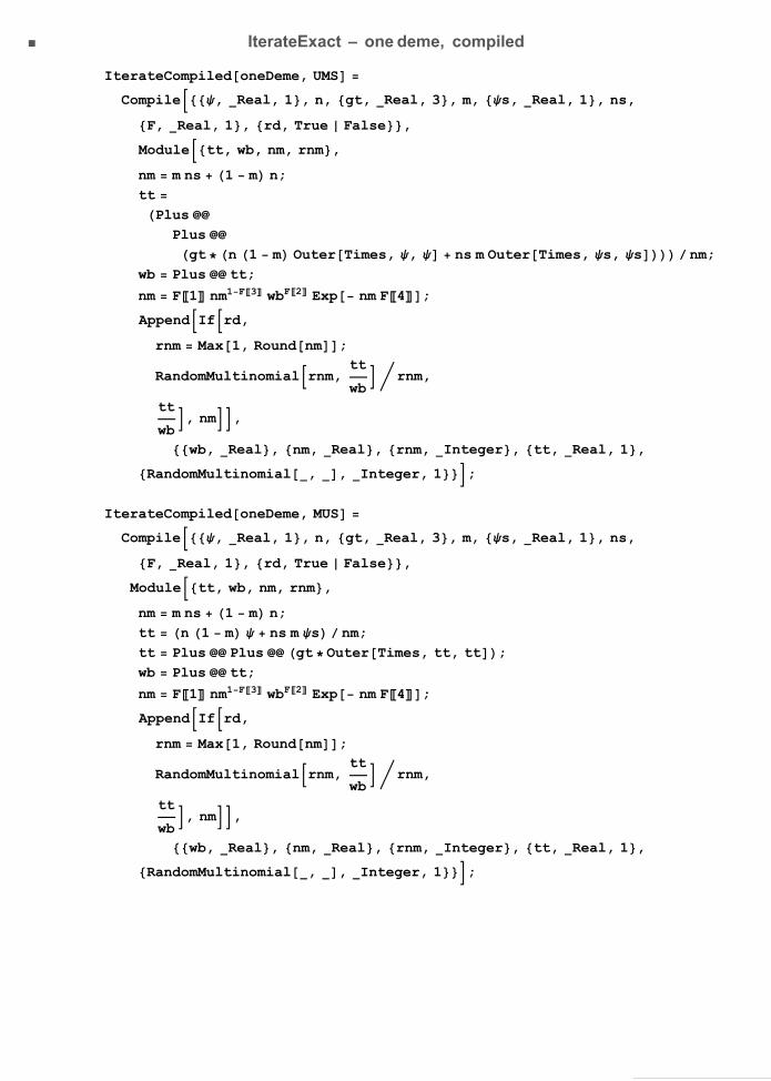
IterateExact one deme, compiled

IterateCompiledoneDeme, UMS Compile, Real, 1, n, gt, Real, 3, m, s, Real, 1, ns,F, Real, 1, rd, True False,

Modulett, wb, nm, rnm,nm m ns 1 mn;tt Plus

Plus gt n1 mOuterTimes, , ns m OuterTimes, s, snm;wb Plus tt;

nm F1 nm1F3wbF2Exp nm F4;AppendIfrd,rnm Max1, Roundnm;RandomMultinomialrnm, tt

wb rnm,

tt

wb, nm,wb, Real, nm, Real, rnm, Integer, tt, Real, 1,RandomMultinomial, , Integer, 1;

IterateCompiledoneDeme, MUS Compile, Real, 1, n, gt, Real, 3, m, s, Real, 1, ns,F, Real, 1, rd, True False,Modulett, wb, nm, rnm,nm m ns 1 mn;tt n1 m ns m s nm;tt Plus Plus gt OuterTimes, tt, tt;wb Plus tt;

nm F1 nm1F3wbF2Exp nm F4;AppendIfrd,rnm Max1, Roundnm;RandomMultinomialrnm, tt

wb rnm,

tt

wb, nm,wb, Real, nm, Real, rnm, Integer, tt, Real, 1,RandomMultinomial, , Integer, 1;



IterateCompiledoneDeme, USM Compile, Real, 1, n, gt, Real, 3, m, s, Real, 1, ns,F, Real, 1, rd, True False,Modulett, wb, nn, nnn, rnm,tt Plus Plus gt OuterTimes, , ;wb Plus tt; nn F1 n1F3wbF2Exp n F4;nnn 1 mnn ns m;AppendIfrd,rnm Max1, Roundnnn;RandomMultinomialrnm, nn1 m tt

wb ns m s

nnn rnm,

nn1 m ttwb

ns m s

nnn, nnn,wb, Real, nn, Real, rnm, Integer, nnn, Real,tt, Real, 1, RandomMultinomial, , Integer, 1;

IterateExact one deme, compiled, allele frequencies

IterateCompiledww, oneDeme, UMS :Modulefw,fwp : Flattenwwp;IterateCompiledww, oneDeme, UMS Compilep, Real, 1, n, m, ps, Real, 1, ns, F, Real, 1,rd, True False,Modulewv, np, wb, nm, rnm,nm m ns 1 mn;np

n1 mp ns m ps

nm;

wv fwnp; wb wv1;np np 1 1 npDropwv, 1

wb;

nm F1 nm1F3wbF2Exp nm F4;AppendIfrd,rnm Max1, Roundnm;FirstRandomMultinomialrnm, , 1 & np rnm,np,nm,wv, Real, 1, np, Real, 1, wb, Real, nm, Real,rnm, Integer, RandomMultinomial, , Integer, 1,fw, Real, 1;

IterateCompiledww, oneDeme, MUS : IterateCompiledww, oneDeme, UMS;



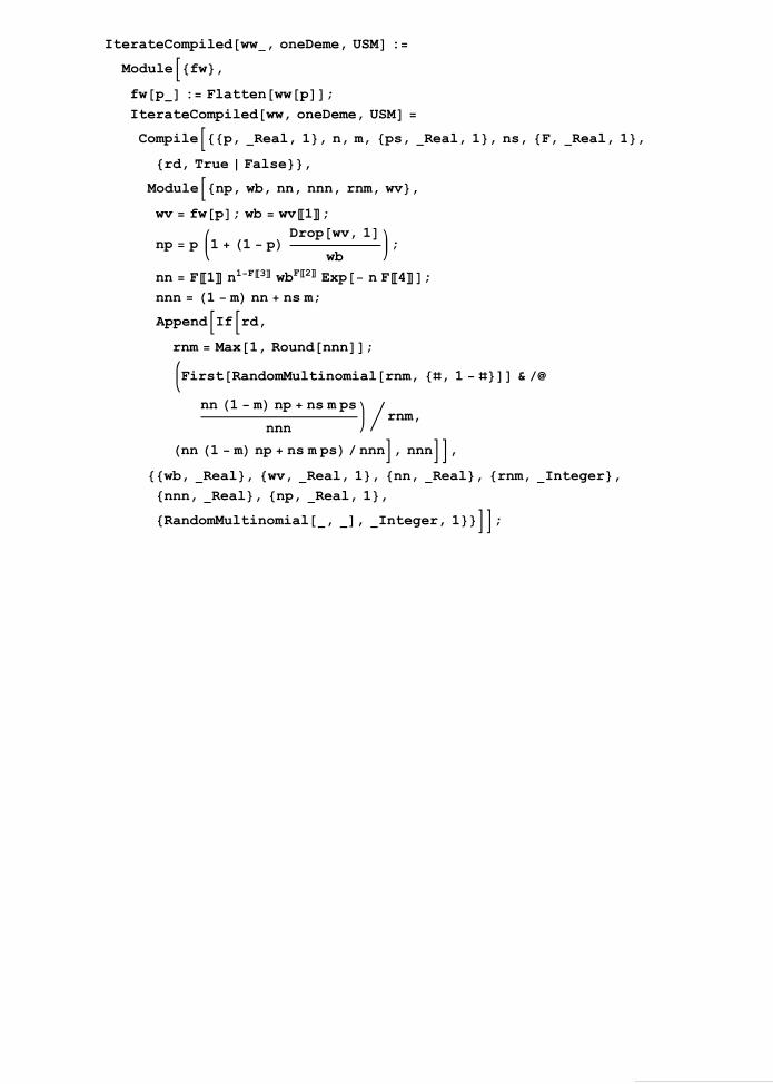
IterateCompiledww, oneDeme, USM :Modulefw,fwp : Flattenwwp;IterateCompiledww, oneDeme, USM Compilep, Real, 1, n, m, ps, Real, 1, ns, F, Real, 1,rd, True False,Modulenp, wb, nn, nnn, rnm, wv,wv fwp; wb wv1;np p 1 1 pDropwv, 1

wb;

nn F1 n1F3wbF2Exp n F4;nnn 1 mnn ns m;AppendIfrd,rnm Max1, Roundnnn;FirstRandomMultinomialrnm, , 1 &

nn1 mnp ns m psnnn

rnm,nn1 mnp ns m ps nnn, nnn,wb, Real, wv, Real, 1, nn, Real, rnm, Integer,nnn, Real, np, Real, 1,RandomMultinomial, , Integer, 1;



IterateExact cline, compiled

IterateCompiledcline, UMS Compile, Real, 2, nl, Real, 1, gt, Real, 4, m,fe0, Real, 1, fe1, Real, 1, n0, n1, F, Real, 2,rd, True False, Module, n, nn, tt, i, nm, wb, rnm, nnm, OuterTimes, , & ; PrependAppend,

IfLengthfe1 0, Last, OuterTimes, fe1, fe1,IfLengthfe0 0, First, OuterTimes, fe0, fe0;

nn PrependAppendnl,IfLengthfe1 0, Lastnl, n1,

IfLengthfe0 0, Firstnl, n0; n nn ;

n DropDrop1 mn m

2RotateLeftn RotateRightn, 1,

1;nm DropDrop1 mnn m

2RotateLeftnn RotateRightnn, 1, 1;

Tablett Plus Plus gti ni nmi; wb Plus tt;nnm Fi, 1 nmi1Fi,3wbFi,2Exp nmi Fi, 4;rnm Ifrd, RandomRealPoissonDistributionnnm,

Max1, Roundnnm;AppendIfrd, RandomMultinomialrnm, tt

wb rnm,

tt

wb, nnm,i, Length,tt, Real, 1, nm, Real, 1, wb, Real, nn, Real, 1,, Real, 3, n, Real, 3, i, Integer,RandomMultinomial, , Integer, 1,RandomRealPoissonDistribution, Integer, rnm, Integer,nnm, Real;



IterateCompiledcline, MUS Compile, Real, 2, nl, Real, 1, gt, Real, 4, m,fe0, Real, 1, fe1, Real, 1, n0, n1, F, Real, 2,rd, True False, Module, y, ny, nn, nm, nnm, rnm, tt, wb,

y PrependAppend,IfLengthfe1 0, Last, fe1,IfLengthfe0 0, First, fe0;

nn PrependAppendnl,IfLengthfe1 0, Lastnl, n1,IfLengthfe0 0, Firstnl, n0;

ny nn y;

ny DropDrop1 mny m

2RotateLeftny RotateRightny, 1,


2RotateLeftnn RotateRightnn, 1,

1; OuterTimes, , & nynm

;Tablett Plus Plus gti i; wb Plus tt;

nnm Fi, 1 wbFi,2nmi1Fi,3Exp nmi Fi, 4;rnm Ifrd, RandomRealPoissonDistributionnnm,

Max1, Roundnnm;AppendIfrd, RandomMultinomialrnm, tt

wb rnm,

tt

wb, nnm,i, Length , nn, Real, 1, nm, Real, 1, wb, Real,tt, Real, 1, y, Real, 2, ny, Real, 2, , Real, 3,i, Integer, RandomMultinomial, , Integer, 1,RandomRealPoissonDistribution, Integer, rnm, Integer,nnm, Real;



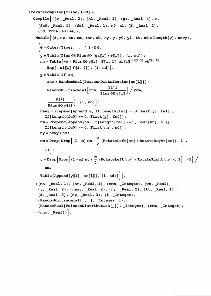
IterateCompiledcline, USM Compile, Real, 2, nl, Real, 1, gt, Real, 4, m,fe0, Real, 1, fe1, Real, 1, n0, n1, F, Real, 2,rd, True False,Module, n, nn, nm, rnm, wb, ny, y, y0, y1, tt, nd Length, newy, OuterTimes, , & ;y TablePlus Plus gti i, i, nd;nn Tablewb Plus yi; Fi, 1 nli1Fi,3wbFi,2

Exp nli Fi, 4, i, nd;y TableIfrd,

rnm RandomRealPoissonDistributionnni;RandomMultinomialrnm, yi

Plus yi rnm,

yiPlus yi, i, nd;

newy PrependAppendy, IfLengthfe1 0, Lasty, fe1,IfLengthfe0 0, Firsty, fe0;

nm PrependAppendnn, IfLengthfe1 0, Lastnn, n1,IfLengthfe0 0, Firstnn, n0;

ny newy nm;

nm DropDrop1 mnm m

2RotateLeftnm RotateRightnm, 1,

1;y DropDrop1 mny m

2RotateLeftny RotateRightny, 1, 1

nm;

TableAppendyi, nmi, i, nd ,nn, Real, 1, nm, Real, 1, rnm, Integer, wb, Real,y, Real, 2, newy, Real, 2, ny, Real, 2, tt, Real, 1,, Real, 3, n, Real, 3, i, Integer,RandomMultinomial, , Integer, 1,RandomRealPoissonDistribution, Integer, rnm, Integer,nnm, Real;



IterateExact cline, compiled, allele frequencies

IterateCompiledww, cline, UMS : Modulefw,fwp, d : Flattenwwdp;IterateCompiledww, cline, UMS Compile, Real, 2, nl, Real, 1, m, fe0, Real, 1,fe1, Real, 1, n0, n1, F, Real, 2, rd, True False,Modulen, nn, np, tt, i, nm, wb, rnm, nnm, wv, n,n PrependAppend,

IfLengthfe1 0, Last, fe1,IfLengthfe0 0, First, fe0; nn PrependAppendnl,IfLengthfe1 0, Lastnl, n1,IfLengthfe0 0, Firstnl, n0; n nnn;

n DropDrop1 mn m




1; Tablenp ninmi; wv fwnp, i; wb wv1;

np np 1 1 npDropwv, 1wb

;

nnm Fi, 1 nmi1Fi,3wbFi,2Exp nmi Fi, 4;AppendIfrd,rnm Max1, Roundnnm;FirstRandomMultinomialrnm, , 1 & np rnm,np, nnm, i, Length,n, Real, 2, wv, Real, 1, nm, Real, 1,wb, Real, nn, Real, 1, np, Real, n, Real, 3,i, Integer, RandomMultinomial, , Integer, 1,rnm, Integer, nnm, Real, fw, , Real, 1;

IterateCompiledww, cline, MUS : IterateCompiledww, cline, UMS;



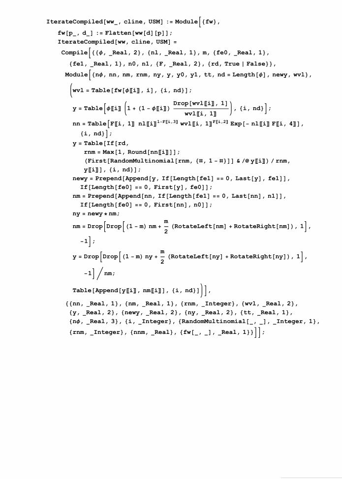
IterateCompiledww, cline, USM : Modulefw,fwp, d : Flattenwwdp;IterateCompiledww, cline, USM Compile, Real, 2, nl, Real, 1, m, fe0, Real, 1,fe1, Real, 1, n0, n1, F, Real, 2, rd, True False,Modulen, nn, nm, rnm, ny, y, y0, y1, tt, nd Length, newy, wvl,wvl Tablefwi, i, i, nd;y Tablei 1 1 iDropwvli, 1

wvli, 1 , i, nd;nn TableFi, 1 nli1Fi,3wvli, 1Fi,2Exp nli Fi, 4,i, nd;y TableIfrd,

rnm Max1, Roundnni;FirstRandomMultinomialrnm, , 1 & yi rnm,yi, i, nd;

newy PrependAppendy, IfLengthfe1 0, Lasty, fe1,IfLengthfe0 0, Firsty, fe0;

nm PrependAppendnn, IfLengthfe1 0, Lastnn, n1,IfLengthfe0 0, Firstnn, n0;

ny newy nm;

nm DropDrop1 mnm m


1;y DropDrop1 mny m


1 nm;

TableAppendyi, nmi, i, nd ,nn, Real, 1, nm, Real, 1, rnm, Integer, wvl, Real, 2,y, Real, 2, newy, Real, 2, ny, Real, 2, tt, Real, 1,n, Real, 3, i, Integer, RandomMultinomial, , Integer, 1,rnm, Integer, nnm, Real, fw, , Real, 1;



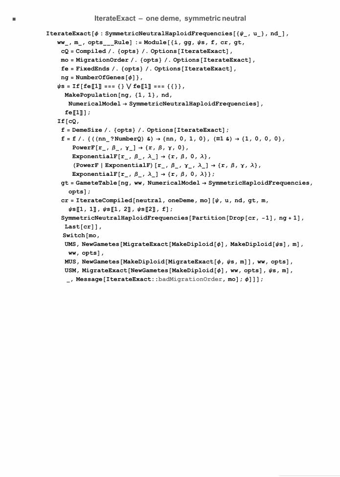
IterateExact one deme, symmetric neutral

IterateExact : SymmetricNeutralHaploidFrequencies, u, nd,ww, m, optsRule : Modulei, gg, s, f, cr, gt,cQ Compiled . opts . OptionsIterateExact,mo MigrationOrder . opts . OptionsIterateExact,fe FixedEnds . opts . OptionsIterateExact,ng NumberOfGenes,s Iffe1 fe1 ,

MakePopulationng, 1, 1, nd,NumericalModel SymmetricNeutralHaploidFrequencies,fe1;

IfcQ,f DemeSize . opts . OptionsIterateExact;f f . nn?NumberQ & nn, 0, 1, 0, 1 & 1, 0, 0, 0,

PowerFr, , r, , , 0,ExponentialFr, , r, , 0, ,PowerF ExponentialFr, , , r, , , ,ExponentialFr, , r, , 0, ;

gt GameteTableng, ww, NumericalModel SymmetricHaploidFrequencies,opts;

cr IterateCompiledneutral, oneDeme, mo, u, nd, gt, m,s1, 1, s1, 2, s2, f;

SymmetricNeutralHaploidFrequenciesPartitionDropcr, 1, ng 1,Lastcr,Switchmo,UMS, NewGametesMigrateExactMakeDiploid, MakeDiploids, m,ww, opts,MUS, NewGametesMakeDiploidMigrateExact, s, m, ww, opts,USM, MigrateExactNewGametesMakeDiploid, ww, opts, s, m,, MessageIterateExact::badMigrationOrder, mo; ;



IterateExact one deme, compiled, symmetric neutral

IterateCompiledneutral, oneDeme, UMS Compile, Real, 1, u, Real, 1, n, gt, Real, 3, m,s, Real, 1, us, Real, 1, ns, F, Real, 1,

Modulett, ttu, wb, nm,nm m ns 1 mn;tt Plus

Plus gt n1 mOuterTimes, , ns m OuterTimes, s, snm;ttu Plus

Plus gt n1 mOuterTimes, , OuterPlus, u, u ns m OuterTimes, s, sOuterPlus, us, us 2nm;

wb Plus tt;

nm F1 nm1F3wbF2Exp nm F4;AppendJointt

wb, DivideZerottu, tt, nm,wb, Real, nm, Real, tt, Real, 1, ttu, Real, 1,DivideZero, , Real, 1;

IterateCompiledneutral, oneDeme, MUS Compile, Real, 1, u, Real, 1, n, gt, Real, 3, m,s, Real, 1, us, Real, 1, ns, F, Real, 1,Modulett, ttu, wb, nm, nu, ngt,nm m ns 1 mn;tt n1 m ns m s nm;ttu n1 m u ns m s us nm;nu DivideZerottu, tt;ngt gt OuterTimes, tt, tt;tt Plus Plus ngt;ttu Plus Plus ngt OuterPlus, nu, nu 2;wb Plus tt;

nm F1 nm1F3wbF2Exp nm F4;AppendJointt

wb, DivideZerottu, tt, nm,wb, Real, nm, Real, tt, Real, 1, ttu, Real, 1,ngt, Real, 3, nu, Real, 1, DivideZero, , Real, 1;



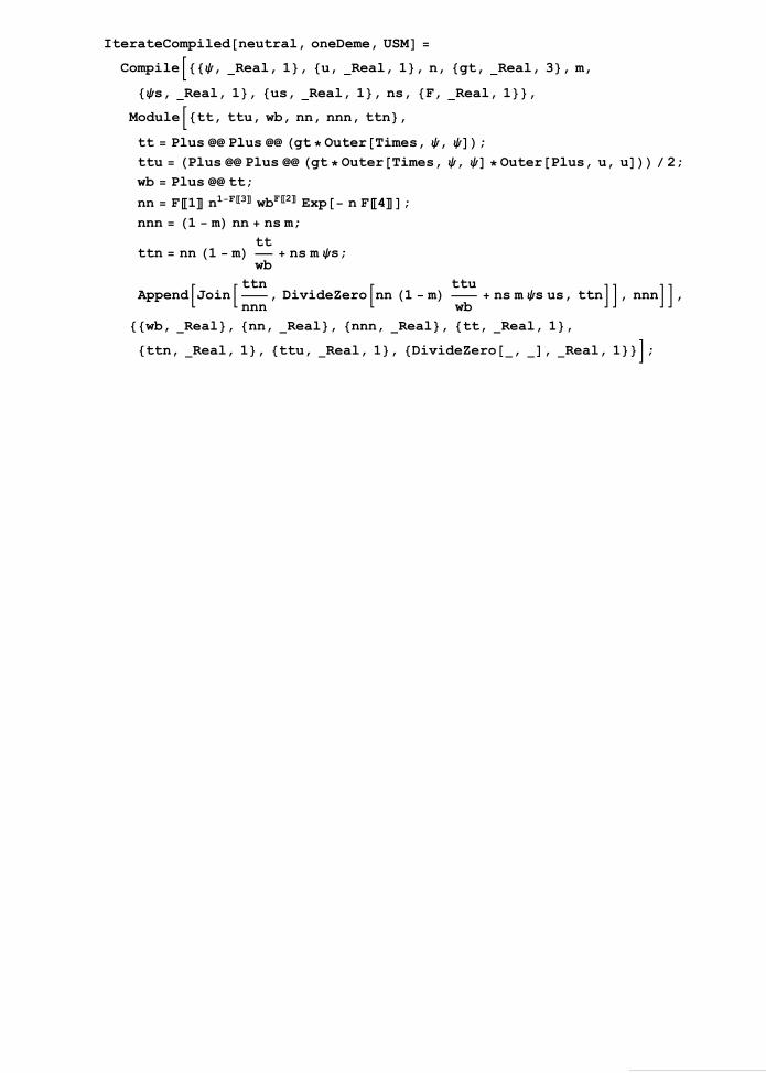
IterateCompiledneutral, oneDeme, USM Compile, Real, 1, u, Real, 1, n, gt, Real, 3, m,s, Real, 1, us, Real, 1, ns, F, Real, 1,Modulett, ttu, wb, nn, nnn, ttn,tt Plus Plus gt OuterTimes, , ;ttu Plus Plus gt OuterTimes, , OuterPlus, u, u 2;wb Plus tt;

nn F1 n1F3wbF2Exp n F4;nnn 1 mnn ns m;ttn nn1 mtt

wb ns m s;

AppendJointtnnnn

, DivideZeronn1 mttuwb

ns m s us, ttn, nnn,wb, Real, nn, Real, nnn, Real, tt, Real, 1,ttn, Real, 1, ttu, Real, 1, DivideZero, , Real, 1;



IterateExact cline, symmetric neutral

IterateExact : SymmetricNeutralHaploidFrequencies, , ..,ww, m, opts :Modulei, gg, nd Length, cr, gt, 0, 1, u0, u1, n0, n1,cQ Compiled . opts . OptionsIterateExact,mo MigrationOrder . opts . OptionsIterateExact,fe FixedEnds . opts . OptionsIterateExact,, u, nl, dsrl,ng NumberOfGenes,IfcQ, First First ;u Last First ;nl Last ;f DemeSize . opts . OptionsIterateExact;f f . nn?NumberQ & Arraynn, 0, 1, 0 &, nd,1 & Array1, 0, 0, 0 &, nd,

PowerFr, , Arrayr, , , 0 &, nd,ExponentialFr, , Arrayr, , 0, &, nd,PowerF ExponentialFr, , , Arrayr, , , &, nd,ExponentialFr, , Arrayr, , 0, &, nd;

Iffe1 ,0 ; u0 ; n0 0,0 fe1, 1, 1; u0 fe1, 1, 2; n0 fe1, 2;Iffe1 ,1 ; u1 ; n1 0,1 fe1, 1, 1; u1 fe1, 1, 2; n1 fe1, 2;

gt TableGameteTableng, wwi,NumericalModel SymmetricNeutralHaploidFrequencies, opts,i, nd;

cr IterateCompiledneutral, cline, mo, u, nl, gt, m, 0,1, u0, u1, n0, n1, f;

SymmetricNeutralHaploidFrequenciesPartitionDrop, 1, ng 1,Last & cr,

dsrlj : DemeSize f?NotListQ & DemeSize fj,DemeSize fList DemeSize fj;Switchmo,UMS,gg MigrateExactMakeDiploid, m, FixedEnds MakeDiploid fe;TableNewGametesggi, wwi, & opts . dsrli, i, nd,MUS,gg MakeDiploidMigrateExact, m, FixedEnds fe;TableNewGametesggi, wwi, & opts . dsrli, i, nd,USM,gg MakeDiploid;MigrateExactTableNewGametesggi, wwi, & opts . dsrli, i, nd, m, FixedEnds fe,,MessageIterateExact::badMigrationOrder, mo;SymmetricNeutralHaploidFrequencies, n;



IterateExact cline, compiled, symmetric neutral

IterateCompiledneutral, cline, UMS Compile, Real, 2, u, Real, 2, nl, Real, 1, gt, Real, 4,m, fe0, Real, 1, fe1, Real, 1, feU0, Real, 1,feU1, Real, 1, n0, n1, F, Real, 2,Module, u, n, nu, nn, tt, ttu, nu, i, nm, wb, nnm, OuterTimes, , & ;u MapThreadOuterTimes, 1, 1OuterPlus, 2, 2 &, , u 2; PrependAppend,

IfLengthfe1 0, Last, OuterTimes, fe1, fe1,IfLengthfe0 0, First, OuterTimes, fe0, fe0;

u PrependAppendu,IfLengthfe1 0, Lastu,OuterTimes, fe1, fe1OuterPlus, feU1, feU1 2,

IfLengthfe0 0, Firstu,OuterTimes, fe0, fe0OuterPlus, feU0, feU0 2;

nn PrependAppendnl,IfLengthfe1 0, Lastnl, n1,

IfLengthfe0 0, Firstnl, n0;n nn ; nu nn u;

n DropDrop1 mn m


1;nu DropDrop1 mnu m

2RotateLeftnu RotateRightnu, 1,


2RotateLeftnn RotateRightnn, 1, 1;

nu MapThreadDivideZero1, 2 &, nu, n, 2;Tablett Plus Plus gti ninmi;ttu Plus Plus gti ni nui nmi;wb Plus tt;

nnm Fi, 1 nmi1Fi,3wbFi,2Exp nmi Fi, 4;AppendJointt

wb, DivideZerottu, tt, nnm,i, Length,tt, Real, 1, ttu, Real, 1, nm, Real, 1,wb, Real, nn, Real, 1, , Real, 3, u, Real, 3,nu, Real, 3, n, Real, 3, nu, Real, 3, i, Integer,nnm, Real, DivideZero, , Real, 1;



IterateCompiledneutral, cline, MUS Compile, Real, 2, u, Real, 2, nl, Real, 1, gt, Real, 4,m, fe0, Real, 1, fe1, Real, 1, feU0, Real, 1,feU1, Real, 1, n0, n1, F, Real, 2,Module, u, y, yu u, ny, nyu, nn, nm, nnm, tt, ttu, wb,y PrependAppend,

IfLengthfe1 0, Last, fe1,IfLengthfe0 0, First, fe0;

yu PrependAppendyu,IfLengthfe1 0, Lastyu, fe1 feU1,IfLengthfe0 0, Firstyu, fe0 feU0;

nn PrependAppendnl,IfLengthfe1 0, Lastnl, n1,IfLengthfe0 0, Firstnl, n0;

ny nn y; nyu nn yu;

ny DropDrop1 mny m


1;nyu DropDrop1 mnyu m

2RotateLeftnyu RotateRightnyu, 1,



1; ny ny nm;nyu MapThreadDivideZero1, 2 &, nyu, ny; OuterTimes, , & ny;u MapThreadOuterTimes, 1, 1OuterPlus, 2, 2

2&, ny, nyu;

Tablett Plus Plus gti i;ttu Plus Plus gti ui;wb Plus tt;

nnm Fi, 1 wbFi,2nmi1Fi,3Exp nmi Fi, 4;AppendJointt

wb, DivideZerottu, tt, nnm, i, Length ,nn, Real, 1, nm, Real, 1, wb, Real, tt, Real, 1,ttu, Real, 1, y, Real, 2, yu, Real, 2, ny, Real, 2,nyu, Real, 2, , Real, 3, u, Real, 3, i, Integer,DivideZero, , Real, 1, nnm, Real;



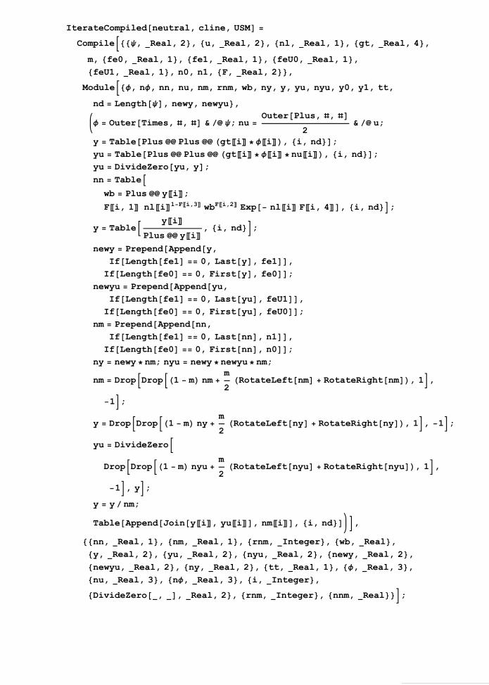
IterateCompiledneutral, cline, USM Compile, Real, 2, u, Real, 2, nl, Real, 1, gt, Real, 4,m, fe0, Real, 1, fe1, Real, 1, feU0, Real, 1,feU1, Real, 1, n0, n1, F, Real, 2,Module, n, nn, nu, nm, rnm, wb, ny, y, yu, nyu, y0, y1, tt,

nd Length, newy, newyu, OuterTimes, , & ; nu OuterPlus, ,

2& u;

y TablePlus Plus gti i, i, nd;yu TablePlus Plus gti i nui, i, nd;yu DivideZeroyu, y;nn Tablewb Plus yi;Fi, 1 nli1Fi,3wbFi,2Exp nli Fi, 4, i, nd;

y Table yiPlus yi, i, nd;

newy PrependAppendy,IfLengthfe1 0, Lasty, fe1,IfLengthfe0 0, Firsty, fe0;

newyu PrependAppendyu,IfLengthfe1 0, Lastyu, feU1,IfLengthfe0 0, Firstyu, feU0;

nm PrependAppendnn,IfLengthfe1 0, Lastnn, n1,IfLengthfe0 0, Firstnn, n0;

ny newy nm; nyu newy newyu nm;

nm DropDrop1 mnm m


1;y DropDrop1 mny m

2RotateLeftny RotateRightny, 1, 1;

yu DivideZeroDropDrop1 mnyu m

2RotateLeftnyu RotateRightnyu, 1,

1, y;y y nm;TableAppendJoinyi, yui, nmi, i, nd ,nn, Real, 1, nm, Real, 1, rnm, Integer, wb, Real,y, Real, 2, yu, Real, 2, nyu, Real, 2, newy, Real, 2,newyu, Real, 2, ny, Real, 2, tt, Real, 1, , Real, 3,nu, Real, 3, n, Real, 3, i, Integer,DivideZero, , Real, 2, rnm, Integer, nnm, Real;



Lligam::usage "LligamSubscriptBoxr, 1, \ 2,SubscriptBoxr,2, 3,… isan option for Gametes, GameteTable and RandomFamilywhich specifies the recombination rates in each interval;assumes no interference and a linear map. The defaultLinkageFalse gives unlinked loci. ";

MakeCline

MakeCline::usage "MakeClinendemes,nloci,ninds sets up a stepped cline, withninds individuals per deme. MakeClinendemes,nloci,ninds,dpsets up a linear gradient, with net change dp1.NumericalModel specifies which representation is to beused. SymmetricNeutralModel allows for the presence of aneutral locus under the symmetric model; this is initiallyeither in a step, or a gradient spanning dp. ";

OptionsMakeCline NumericalModel HaploidFrequencies;MakeClinend, ng, ni, optsRule :Modulenm NumericalModel . opts . OptionsMakeCline,

pp Array12 1 Sign nd 1

2 &, nd,

MakePopulationng, , ni, opts & Switchnm,NonNeutralRepresentations, pp,NeutralRepresentations, Transposepp, pp,, MessageNumericalModel::badSetting, nm; ;

MakeClinend, ng, ni, dp, optsRule :Modulenm NumericalModel . opts . OptionsMakeCline,

pp Range1 dp2

,1 dp

2,

dp

nd 1,

MakePopulationng, , ni, opts & Switchnm,NonNeutralRepresentations, pp,NeutralRepresentations, Transposepp, pp,, MessageNumericalModel::badSetting, nm; ;

MakeDiploid

MakeDiploid::usage "MakeDiploidHaploidFrequencies… gives the matrix of diploidgenotype frequencies after random mating. Deme size ishalved. Applies to vectors of class, genotype and allelefrequencies; MakeDiploidHaploidIndividuals… generatesa population of diploids by sampling with replacementfrom the haploid population; not particularly useful, andadded for completeness only.";



MakeDiploid::odd "MakeDiploidHaploidIndividuals,n only applies when n iseven. Deme size `1` has been reduced by 1.";

MakeDiploid : PopulationRepresentations, ... : MakeDiploid ;MakeDiploid : DiploidRepresentations, : ;MakeDiploidHaploidFrequencies, n :DiploidFrequenciesOuterTimes, , , n 2;

MakeDiploidSymmetricHaploidFrequencies, n :SymmetricDiploidFrequenciesOuterTimes, , , n 2;

MakeDiploidSymmetricNeutralHaploidFrequencies, u, n :SymmetricNeutralDiploidFrequenciesOuterTimes, , , MidParentu,n 2;

MakeDiploidHaploidIndividuals, n?OddQ :MessageMakeDiploid::odd, n;DiploidIndividualsPartitionDrop, 1, 2, n 1 2;

MakeDiploidHaploidIndividuals, n?EvenQ :DiploidIndividualsPartition, 2, n 2;

MakeHaploid

MakeHaploid::usage "MakeHaploidDiploidFrequencies… gives the haploid genotypefrequencies, averaged over maternal and paternal genomes.Deme size is doubled. Applies to vectors of class,genotype and allele frequencies. Deme size is leftunaltered, except for MakeHaploidDiploidIndividuals…,for which deme size is doubled. This just flattens thelist: there is no sampling.";

MakeHaploid : DiploidRepresentations, ... : MakeHaploid ;MakeHaploidDiploidFrequencies, n :HaploidFrequenciesPlus Plus Transpose 2, 2n;

MakeHaploidAlleleFrequenciesp, n : AlleleFrequenciesp, 2n;MakeHaploidSymmetricDiploidFrequencies, n :SymmetricHaploidFrequenciesPlus Plus Transpose 2, 2n;

MakeHaploidSymmetricNeutralDiploidFrequencies, u, n :Modulem Plus Plus Transpose2, u u,SymmetricNeutralHaploidFrequenciesm, Plus u Plus Transposeu 2m, 2n;

MakeHaploidDiploidIndividuals, n :HaploidIndividualsFlatten, 1, 2n;



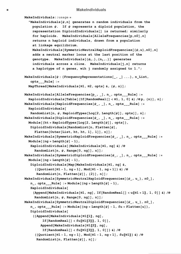
MakeIndividuals

MakeIndividuals::usage "MakeIndividuals,n generates n random individuals from thepopulation . If represents a diploid population, therepresentation DiploidIndividuals is returned; similarlyfor haploids. MakeIndividualsAlleleFrequenciesp,n0,nreturns n haploid individuals, drawn from a populationat linkage equilibrium.MakeIndividualsSymmetricNeutralHaploidFrequencies,u,n0,nadds a neutral marker locus at the last position of thegenotype. MakeIndividuals1…,n1,… generatesindividuals across a cline. MakeIndividualsj,n returnsa haplotype of n genes, wih j randomly assigned to 1.";

MakeIndividuals : FrequencyRepresentations, ..., nList,optsRule :MapThreadMakeIndividuals1, 2, opts &, , n;

MakeIndividualsAlleleFrequenciesp, , n, optsRule :HaploidIndividualsTableIfRandomReal 1, 1, 0 & p, n, n;

MakeIndividualsHaploidFrequencies, , n, optsRule :HaploidIndividualsRandomListn, , HaploidTypesLog2, Length, opts, n;

MakeIndividualsDiploidFrequencies, , n, optsRule :Moduleht HaploidTypesLog2, Length, opts,DiploidIndividualsRandomListn, Flatten,FlattenOuterList, ht, ht, 1, 1, n;

MakeIndividualsSymmetricHaploidFrequencies, , n, optsRule :Moduleng Length 1,HaploidIndividualsMakeIndividuals1, ng & RandomListn, , Range0, ng, n;

MakeIndividualsSymmetricDiploidFrequencies, , n, optsRule :Moduleng Length 1,DiploidIndividualsMapMakeIndividuals1, ng &,Quotient1 1, ng 1, Mod1 1, ng 1 &

RandomListn, Flatten, 2, n;MakeIndividualsSymmetricNeutralHaploidFrequencies, u, n0,

n, optsRule : Moduleng Length 1,HaploidIndividualsAppendMakeIndividuals1, ng, IfRandomReal u1 1, 1, 0 & RandomListn, , Range0, ng, n;

MakeIndividualsSymmetricNeutralDiploidFrequencies, u, n0,n, optsRule : Moduleng Length 1, fu Flattenu,DiploidIndividualsAppendMakeIndividuals11, ng,

IfRandomReal fu13, 1, 0,AppendMakeIndividuals12, ng,IfRandomReal fu13, 1, 0 & Quotient1 1, ng 1, Mod1 1, ng 1, fu1 &

RandomListn, Flatten, n;



MakeIndividualsjInteger, nInteger :MuddleJoinArray1 &, j, Array0 &, n j;

MakeOptionsHaploid

MakeOptionsHaploid::usage "MakeOptionsHaploid is a rule which converts options such asNumericalModelDiploidFrequencies to their haploid version";

MakePopulation

MakePopulation::usage "MakePopulationnloci,p gives a haploid population at linkageequilibrium, with allele frequency p; this is representedas HaploidFrequencies000…. The option NumericalModelcan be used to give other representations. For example,MakePopulationnloci,p,u,NumericalModelSymmetricNeutralHaploidFrequencies gives a haploidpopulation at LE, with selected loci at frequency p, anda single neutral marker at frequency u.MakePopulationnloci,p,NumericalModelHaploidIndividualsgives a single haploid individual, drawn at random.MakePopulationnloci,p,ndeme,opts allows deme size tobe specified; the default is 1. ";

OptionsMakePopulation NumericalModel HaploidFrequencies, SortByClass False;MakePopulationnlociInteger, p, optsRule :MakePopulationnloci, p, 1, opts;



MakePopulationnInteger, p, ninds, optsRule :Modulei, nm NumericalModel . opts . OptionsMakePopulation,Switchnm,HaploidRepresentations,

Switchnm,HaploidFrequencies,HaploidFrequenciesHaploidTypesn, opts .aInteger : Times a2p 1 1 p, ninds,

SymmetricHaploidFrequencies,

SymmetricHaploidFrequenciesIfp 0,ReplacePartArray0 &, n 1, 1, 1,Ifp 1,ReplacePartArray0 &, n 1, 1, 1,

TableBinomialn, ipi1 pni, i, 0, n, ninds,SymmetricNeutralHaploidFrequencies,SymmetricNeutralHaploidFrequenciesMakePopulationn, p1, NumericalModel

SymmetricHaploidFrequencies1, Arrayp2 &, n 1, ninds,AlleleFrequencies,AlleleFrequenciesArray1 &, np, ninds,

HaploidIndividuals,

MakeIndividuals AlleleFrequenciesArray1 &, np, 1, ninds,DiploidRepresentations,Switchnm,DiploidIndividuals,DiploidIndividualsTranspose

MakePopulationn, p, ninds, NumericalModel HaploidIndividuals1,MakePopulationn, p, ninds, NumericalModel HaploidIndividuals1, ninds,

,MakeDiploidMakePopulationn, p, ninds, & opts . MakeOptionsHaploid,

,MessageNumericalModel::badSetting, nm; ; Mendel

Mendel::usage "Mendel0,1,…,1,0,… gives a random gamete, assumingno linkage.";

Mendelpp : , : Mendel Transposepp;Mendelx, y : IfRandomRealInteger 0, x, y



MeanW

MeanW::usage "MeanW,W gives the mean fitness of population ; W is thefitness function. MeanW,SubscriptBoxW,0, 0,0,… gives the mean fitness, based on an appropriatetable of fitnesses.";

AlleleFrequencies::badW "Wp`1` does not have the form W,s1…";MeanW : PopulationRepresentations, ..., W?NotListQ &,

optsRule :MapIndexedMeanW1, WFirst2, opts &, ;

MeanW : PopulationRepresentations, ..., WList, optsRule :MapIndexedMeanW1, WFirst2, opts &, ;

MeanWSymmetricNeutralHaploidFrequencies, u, n, W,optsRule :MeanWSymmetricHaploidFrequencies, n, W, opts;

MeanWSymmetricNeutralDiploidFrequencies, u, , W,optsRule :MeanWSymmetricDiploidFrequencies, n, W, opts;

MeanWAlleleFrequenciesp, , W?NotListQ &, optsRule :Modulewl Wp,IfMatchQwl, , List,Firstwl,MessageAlleleFrequencies::badW, wl; Indeterminate;

MeanWfr : FrequencyRepresentations, , W?NotListQ &,optsRule :Modulen Switchfr,

SymmetricRepresentations, Length 1,, Log2, Length,

Plus Plus FitnessTableW, n, NumericalModel fr, opts;MeanWHaploidIndividuals, , W?NotListQ &, optsRule :MeanW ;

MeanWDiploidIndividuals, , W?NotListQ &, optsRule :MeanW & ;



MeanWAlleleFrequenciesp, , WList, optsRule :MessageFitnessTable::badOption; 1;MeanWFrequencyRepresentations, , WList, optsRule :Plus Plus W;

MeanWHaploidIndividuals, , WList, optsRule :Moduleht,IfLength 0,Indeterminate,ht HaploidTypesLengthFirst, opts;MeanExtractW, & FirstPositionht, & ;

MeanWDiploidIndividuals, , WList, optsRule :Moduleht,IfLength 0,Indeterminate,ht HaploidTypesLength1, 1, opts;MeanExtractW, & FlattenPositionht, 1, Positionht, 2 & ;

MidParent

MidParent::usage "MidParentu gives the matrix of midparental frequencies, uiuj2";

MidParentu : OuterPlus, u, u 2; MigrateExact

MigrateExact::usage "MigrateExact,s,m implements migration from a sourcepopulation s; can be any valid representation of apopulation. MigrateExact1,…,m implements migrationalong a linear cline. The option FixedEnds0, 1 allowsfixed endpoints. Where individuals are involved, eachhas an independent probability of migrating; for a singlepopulation, the parameter m is now the number of individualsimmigrating from the source population, and must be aninteger no greater than the population size. FixedEndsmust now specify a source with given HaploidFrequenciesor DiploidFrequencies.";

OptionsMigrateExact FixedEnds , ;



MigrateExactpr : NeutralRepresentations, u, n,pr : NeutralRepresentationss, us, ns, m, optsRule :prDivideZero1 mn m ns s, 1 mn m ns,DivideZero1 mn u m ns us s, 1 mn m ns s,1 mn m ns;

MigrateExactpr : FrequencyRepresentations, n,pr : PopulationRepresentationss, ns, m, optsRule :prDivideZero1 mn mns s, 1 mn m ns, 1 mn m ns;

MigrateExactir : IndividualRepresentations, n,fr : FrequencyRepresentationss, ns, NmInteger, optsRule :ModulenStay RandomRealBinomialDistributionn, 1

Nm

n, np,

np irMuddleJoinMakeIndividualsfrs, ns, Nm 1,

RandomSetnStay, , nStay Nm;IfMatchQir, HaploidIndividuals OddQnStay Nm,HaploidIndividualsDropnp1, 1, np2 1, np;

MigrateExact : pr : NeutralRepresentations, .., m,optsRule :Modulepp, os,

os FixedEnds . opts . OptionsMigrateExact;Ifos 1 os 1 , os 1 First;Ifos1 os1 , os1 Last;

pp PrependAppend, Lastos, Firstos;pp pp . NeutralRepresentations, u, n n , n u, n;prDivideZero1, 3, DivideZero2, 1, 3 & DropDrop1 mpp m

2RotateLeftpp RotateRightpp, 1, 1;

MigrateExact : pr : FrequencyRepresentations, .., m,optsRule :Modulepp, os,

os FixedEnds . opts . OptionsMigrateExact;Ifos 1 os 1 , os 1 First;Ifos1 os1 , os1 Last;

pp PrependAppend, Lastos, Firstos;pp pp . FrequencyRepresentations, n n , n;prDivideZero1, 2, 2 & DropDrop1 mpp m

2RotateLeftpp RotateRightpp, 1, 1;



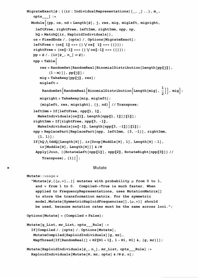
MigrateExact : ir : IndividualRepresentations, .., m,opts :Modulepp, os, nd Length, j, res, mig, migleft, migright,

leftFree, rightFree, leftImm, rightImm, npp, np,hQ MatchQir, HaploidIndividuals,os FixedEnds . opts . OptionsMigrateExact;leftFree os 1 os 1 ;rightFree os1 os1 ;pp . ir, n ;npp Table

res RandomSetRandomRealBinomialDistributionLengthppj,1 m, ppj;mig TakeAwayppj, res;migleft

RandomSetRandomRealBinomialDistributionLengthmig, 1

2, mig;

migright TakeAwaymig, migleft;migleft, res, migright, j, nd Transpose;leftImm IfleftFree, npp1, 1,

MakeIndividualsos1, Lengthnpp1, 11;rightImm IfrightFree, npp3, 1,

MakeIndividualsos1, Lengthnpp3, 11;npp ReplacePartReplacePartnpp, leftImm, 3, 1, rightImm,1, 1;IfhQ OddQLength, irDropMuddle, 1, Length 1,

irMuddle, Length & ApplyJoin, RotateLeftnpp1, npp2, RotateRightnpp3

Transpose, 1; Mutate

Mutate::usage "Mutate,,,… mutates with probability from 0 to 1,and from 1 to 0. CompiledTrue is much faster. Whenapplied to FrequencyRepresentations, uses MutationMatrixto store the transformation matrix. For the symmetricmodel,MutateSymmetricHaploidFrequencies,, shouldbe used, because mutation rates must be the same across loci.";

OptionsMutate Compiled False;MutategList, mrList, optsRule :IfCompiled . opts . OptionsMutate,MutateCompiledHaploidIndividualsg, mr,MapThreadIfRandomReal 21 1, 1 1, 1 &, g, mr;

MutateHaploidIndividuals, n, mrList, optsRule :HaploidIndividualsMutate, mr, opts & , n;



MutateAlleleFrequenciesp, n, mrList, optsRule :AlleleFrequenciesIfCompiled . opts . OptionsMutate,MutateCompiledAlleleFrequenciesp, mr,Moduletmr Transposemr,p1 tmr1 tmr2 tmr1, n;

MutateHaploidFrequencies, n, mrList, optsRule :HaploidFrequenciesConstructMutateMatrixmr, Log2, Length, opts., n;

MutateSymmetricHaploidFrequencies, n, mrList, optsRule :SymmetricHaploidFrequenciesConstructMutateMatrixmr, Length 1, opts,NumericalModel SymmetricHaploidFrequencies., n;

MutateSymmetricNeutralHaploidFrequencies, n, mrList, optsRule :0;

MutateCompiled

MutateCompiled::usage "MutateCompiledHaploidFrequenciesSubscriptBoxp,0,…,…,,,… alters haploid genotype frequencies toallow for mutation.MutateCompiledSymmetricHaploidFrequenciesp0,…,,applies to the symmetric model; similarly forSymmetricNeutralFrequencies. These versions useConstructMutateMatrix to store a large matrix.MutateCompiledAlleleFrequenciesp1,…,,,… appliesto allele frequencies.MutateCompiledHaploidIndividuals0,1,…,,,…mutates a genotype 0,1,… with probability from 0 to1, and from 1 to 0. For short genomes, MutateCompiledis faster than using Mutate…,CompiledTrue, becausethere is no need to check options.";

MutateCompiledHaploidIndividuals Compileg, Integer, 1, mr, Real, 2,Modulej, TableIfRandomReal mrj, gj 1, 1 gj, gj,j, Lengthg, j, Integer;

MutateCompiledAlleleFrequencies Compilep, Real, 1, mr, Real, 2,Moduletmr Transposemr,p1 tmr1 tmr2 tmr1;

MutateCompiledHaploidFrequencies, mr, optsRule :ConstructMutateMatrixmr, Log2, Length, opts, Compiled True.;

MutateCompiledSymmetricHaploidFrequencies, mr :ConstructMutateMatrixmr, Length 1, Compiled True,NumericalModel SymmetricHaploidFrequencies.;



Mutation

Mutation::usage "Mutation,,… is an option for NewGametes which specifiesmutation at rate from 0 to 1, and from 1 to 0.Mutation,… is shorthand for a rate in eachdirection. Mutation, or specifies the samerates at all loci.";

NetRecombinationr1, r2, r3, … gives thenet recombination rate across a linear genetic map

NetRecombination::usage "NetRecombinationr1,r2,r3,… gives the net recombinationrate across a linear genetic map";

NetRecombination : 0;NetRecombinationr, s : s NetRecombinationr1 2s;

NeutralRepresentations

NeutralRepresentations::usage "NeutralRepresentations is a pattern which matchesSymmetricNeutralHaploidFrequenciesSymmetricNeutralDiploidFrequencies.";

NeutralRepresentations SymmetricNeutralHaploidFrequencies SymmetricNeutralDiploidFrequencies;

NewGametes

NewGametes::usage "NewGametes gives the haploid population after meiosis;

must represent a diploid population, or a list of diploidpopulations. By default, deme size is doubled.NewGametes,W does the same, but assuming fitness

function W. DemeSize fn,W allows for changes in deme

size, to 2fn,W. LligamSubscriptBox\r\,\1,\\\\\\\\\\\\ \\\\\\\\\\\\2\\\\,SubscriptBox\r\,\2,\\\\\\\\\\\\ \\\\\\\\\ \\\3\\\\,… canbe used to specify a linear genetic map, where appropriate.RandomDriftTrue samples haploid gametes from the diploidpopulation; does not apply to symmetric or individualrepresentations. TruncationSelectionTrue applies with

individual representations, and takes the fn,W individualswith highest W as parents. Gametes are then sampledrandomly from these parents, so not all the chosen parentsmay actually reproduce. Mutation,,… allows formutation at rate from allele 0 to 1, and from 1 to 0.";

OptionsNewGametes Lligam False, Mutation None, DemeSize 1 &,RandomDrift False, TruncationSelection False;



NewGametes::badN "New deme size `1` is greater than original size `2`";

NewGametesAlleleFrequenciesp, n, optsRule :NewGametesAlleleFrequenciesp, n, 1, Array0 &, Lengthp &, opts;

NewGametespr : DiploidRepresentations, n, optsRule :NewGametespr, n, 1 &, opts;

NewGametesAlleleFrequenciesp, n, W, optsRule :Modulef DemeSize . opts . OptionsNewGametes, ww Wp,rd RandomDrift . opts . OptionsNewGametes, pn,mut Mutation . opts . OptionsNewGametes,f f . r, , , ExponentialFr, , , ;pn AlleleFrequenciesp 1 1 p ww2

ww1 , 2fn, ww1;Ifrd, pn RandomDriftpn, pn2;Ifmut None,pn,

Mutatepn, ConstructMutateListmut, Lengthpn, opts;NewGametesDiploidFrequencies, n, W, optsRule :

Modulef DemeSize . opts . OptionsNewGametes,wb MeanWDiploidFrequencies, n, W, opts,rd RandomDrift . opts . OptionsNewGametes, hn,mut Mutation . opts . OptionsNewGametes,f f . r, , , ExponentialFr, , , ;hn HaploidFrequenciesIfLength 0, ,

If1 ,,Plus Plus GameteTableLog2, Length, W, opts wb,

2fn, wb;Ifrd, hn RandomDrifthn, hn2;Ifmut None,hn,Mutatehn, ConstructMutateListmut, Log2, Length, opts;



NewGametesSymmetricDiploidFrequencies, n, W, optsRule :Modulef DemeSize . opts . OptionsNewGametes,wb MeanWSymmetricDiploidFrequencies, n, W, opts,mut Mutation . opts . OptionsNewGametes,ng, nn,f f . r, , , ExponentialFr, , , ;nn 2fn, wb;IfLength 0,SymmetricHaploidFrequencies, nn,If1 ,SymmetricHaploidFrequencies, nn,ng SymmetricHaploidFrequenciesPlus Plus GameteTableLength 1, W,

NumericalModel SymmetricDiploidFrequencies wb, nn;Ifmut None,ng,Mutateng, mut . , , opts;

NewGametesSymmetricNeutralDiploidFrequencies, u, n, W,optsRule :Modulef DemeSize . opts . OptionsNewGametes,wb MeanWSymmetricNeutralDiploidFrequencies, n, W, opts,gt, n, nu,f f . r, , , ExponentialFr, , , ;SymmetricNeutralHaploidFrequenciesIfLength 0, ,If1 ,,gt GameteTableLength 1, W,NumericalModel SymmetricNeutralDiploidFrequencies;

n Plus Plus gt ;nu Plus Plus gt u;nwb

, DivideZeronu, n,2fn, wb;



NewGametes : DiploidIndividuals, n, W, optsRule :Modulef DemeSize . opts . OptionsNewGametes,wb MeanW, W, opts, wl, newN, rl, ht, tp, np, ss,ts TruncationSelection . opts . OptionsNewGametes,mut Mutation . opts . OptionsNewGametes,wl IfListQW,ht HaploidTypesLength1, 1, opts;ExtractW, & FlattenPositionht, 1, Positionht, 2 & ,W & ;

f f . r, , , ExponentialFr, , , ;newN 2Roundfn, wb;rl Ifts,IfnewN n,MessageNewGametes::badN, newN, n; newN n;

ss Transposewl, Rangen;tp SortwlnewN; np Selectss, 1 tp &;np Joinnp, RandomSetnewN Lengthnp,

Selectss, 1 tp &;MuddleLast np,RandomListnewN, wl

Plus wl;

Ifmut None,HaploidIndividualsRandomFamily, opts & rl, newN,HaploidIndividualsMutateCompiledHaploidIndividualsRandomFamily, opts,

ConstructMutateListmut, Length1, 1 & rl, newN; NonNeutralRepresentations

NonNeutralRepresentations::usage "NonNeutralRepresentations is a pattern which matches anyvalid representation except NeutralRepresentations.";

NonNeutralRepresentations HaploidFrequencies DiploidFrequencies AlleleFrequencies SymmetricHaploidFrequencies SymmetricDiploidFrequencies HaploidIndividuals DiploidIndividuals;

NonSymmetricRepresentations

NonSymmetricRepresentations::usage "NonSymmetricRepresentations is a pattern which matches anyvalid representation except SymmetricRepresentations orAlleleFrequencies.";

NonSymmetricRepresentations HaploidFrequencies DiploidFrequencies HaploidIndividuals DiploidIndividuals;



NumberOfGenes

NumberOfGenes::usage "NumberOfGenes gives the number of genes, where representsa population. Also applies to a list of 's, representinga cline.";

NumberOfGenes::noIndividuals "No individuals in this population";

NumberOfGenespr : PopulationRepresentations, n, :NumberOfGenespr, n;

NumberOfGenespr : PopulationRepresentations, :Switchpr,HaploidFrequencies DiploidFrequencies,Log2, Length,AlleleFrequencies,Length,SymmetricHaploidFrequencies SymmetricDiploidFrequencies,Length 1,SymmetricNeutralHaploidFrequencies SymmetricNeutralDiploidFrequencies,Length1 1,HaploidIndividuals,If , MessageNumberOfGenes::noIndividuals, Length1,DiploidIndividuals,If , MessageNumberOfGenes::noIndividuals, Length1, 1;

NumericalModel

NumericalModel::usage "NumericalModel is an option which determines how a populationis represented. Possible values are anyPopulationRepresentations";

NumericalModel::badSetting "Invalid setting `1` for NumericalModel";

Parents

Parents::usage

"ParentsP returns the parents of each individual in thepedigree. P must be a SparseArray.";

ParentsPSparseArray :Partition1, 2 & DropArrayRulesP . x 2 Sequencex 2, x 2 , 1,

2; PopulationRepresentations

PopulationRepresentations::usage "PopulationRepresentations is a pattern which matches anyvalid representation of a population.";



PopulationRepresentations HaploidFrequencies DiploidFrequencies AlleleFrequencies SymmetricHaploidFrequencies SymmetricDiploidFrequencies SymmetricNeutralHaploidFrequencies SymmetricNeutralDiploidFrequencies HaploidIndividuals DiploidIndividuals;

PowerF

PowerF::usage

"PowerFr,,n,W is the function rSuperscriptBoxn,1 W. DemeSizePowerFr,, can be passed to compiled

versions of IterateExact and StoreExact. PowerFn,0,1n,Wrepresents a fixed number n. PowerFr,,,n,Wrepresents the generalised form rSuperscriptBoxn,1 WExpn. PowerFr…jn,W is the same as PowerFr…n,W.";

PowerFr, , n, wb : rn1wb;

PowerFr, , , n, wb : rn1wbExpn;PowerFr, , n, wb : rn1wb;

PowerFr, , , n, wb : rn1wbExpn; MigrationOrder

MigrationOrder::usage "MigrationOrder is a option for IterateExact which determinesthe order of the life cycle. Can take values UMS, MUS, or USM,";

UMS

UMS::usage "UMS is a setting for MigrationOrder, which represents theorder random unionmigrationselectionmeiosis in IterateExact.";

MUS

MUS::usage "MUS is a setting for MigrationOrder, which represents theorder migrationrandom unionselectionmeiosis in IterateExact.";

USM

USM::usage "USM is a setting for MigrationOrder, which represents theorder random unionselectionmigrationmeiosis in IterateExact.";

RandomDrift

RandomDrift::usage "RandomDrift,n gives the random frequencies generated bysampling n individuals from the genotype or allelefrequencies . CompiledTrue uses compiled code. Demesize is changed to n. RandomDrift, makes no change. ";



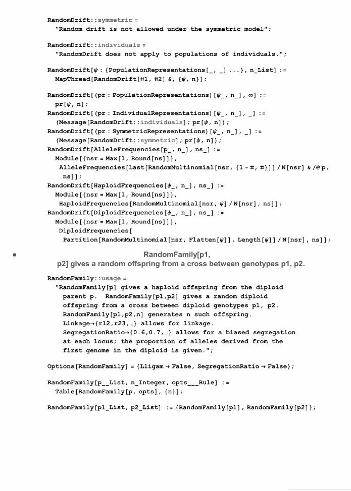
RandomDrift::symmetric "Random drift is not allowed under the symmetric model";

RandomDrift::individuals "RandomDrift does not apply to populations of individuals.";

RandomDrift : PopulationRepresentations, ..., nList :MapThreadRandomDrift1, 2 &, , n;

RandomDriftpr : PopulationRepresentations, n, :pr, n;

RandomDriftpr : IndividualRepresentations, n, :MessageRandomDrift::individuals; pr, n;RandomDriftpr : SymmetricRepresentations, n, :MessageRandomDrift::symmetric; pr, n;RandomDriftAlleleFrequenciesp, n, ns :

Modulensr Max1, Roundns,AlleleFrequenciesLastRandomMultinomialnsr, 1 , Nnsr & p,ns;

RandomDriftHaploidFrequencies, n, ns :Modulensr Max1, Roundns,HaploidFrequenciesRandomMultinomialnsr, Nnsr, ns;

RandomDriftDiploidFrequencies, n, ns :Modulensr Max1, Roundns,DiploidFrequenciesPartitionRandomMultinomialnsr, Flatten, Length Nnsr, ns;

RandomFamily[p1, p2] gives a random offspring from a cross between genotypes p1, p2.

RandomFamily::usage "RandomFamilyp gives a haploid offspring from the diploidparent p. RandomFamilyp1,p2 gives a random diploidoffspring from a cross between diploid genotypes p1, p2.RandomFamilyp1,p2,n generates n such offspring.Linkager12,r23,… allows for linkage.SegregationRatio0.6,0.7,… allows for a biased segregationat each locus; the proportion of alleles derived from thefirst genome in the diploid is given.";

OptionsRandomFamily Lligam False, SegregationRatio False;RandomFamilypList, nInteger, optsRule :TableRandomFamilyp, opts, n;

RandomFamilyp1List, p2List : RandomFamilyp1, RandomFamilyp2;



RandomFamilyp1List, p2List, optsRule :RandomFamilyp1,opts . Lligam xList, yList Lligam x,SegregationRatio xList, yList SegregationRatio x,

RandomFamilyp2,opts . Lligam xList, yList Lligam y,SegregationRatio xList, yList SegregationRatio y;

RandomFamilyh1List, h2List, optsRule :

Modulerl Lligam . opts . OptionsRandomFamily,sr SegregationRatio . opts . OptionsRandomFamily,x, y, tss Transposeh1, h2, j,Ifrl False,Ifsr False, sr Table1

2, Lengthh1;

MapThread1IfRandomReal 2, 1, 2 &,Transposeh1, h2, sr,x RandomRealInteger, 1, 2; y tss1, x;DoIfRandomReal rlj, x Ifx 1, 2, 1;AppendToy, tssj 1, x, j, Lengthrl; y;

SegregationRatio is an option for RandomFamily that specifies the probability that

the allele from the first genome in the diploid is transmitted. SegregationRatio0.6, 0.7, … specifies different ratios for each locus;

SegregationRatio1

2, the default, specifies the same ratio at all loci.

SegregationRatio::usage "SegregationRatio is an option for RandomFamily that specifiesthe probability that the allele from the first genome inthe diploid is transmitted. SegregationRatio0.6,0.7,…specifies different ratios for each locus.SegregationRatio0.6,0.7,…,0.8,… allows different

ratios in the two parents. SegregationRatio1

2, the

default, specifies the same ratio at all loci.";

SortByClass is an option for HaploidTypes[] and Diploid Types[] which determines theorder of the genotypes.

SortByClass::usage "SortByClass is an option for HaploidTypes and DiploidTypes which determines the order of the genotypes.";



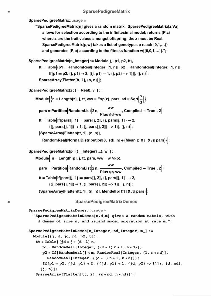
SparsePedigreeMatrix

SparsePedigreeMatrix::usage

"SparsePedigreeMatrixn gives a random matrix. SparsePedigreeMatrixz,Vaallows for selection according to the infinitesimal model; returns P,zwhere z are the trait values amongst offspring; the z must be Real.

SparsePedigreeMatrixp,w takes a list of genotypes p each 0,1,…and generates P,p according to the fitness function w0,0,1,….";

SparsePedigreeMatrixnInteger :Modulej, p1, p2, tt,tt Tablep1 RandomRealInteger, 1, n; p2 RandomRealInteger, 1, n;

Ifp1 p2, j, p1 2, j, p1 1, j, p2 1, j, n;SparseArrayFlattentt, 1, n, n;

SparsePedigreeMatrixz : Real, v :

Modulen Lengthz, j, tt, ww Expz, pars, sd Sqrtv

2,

pars PartitionRandomList2n,ww

Plusww, Compiled True, 2;

tt TableIfparsj, 1 parsj, 2, j, parsj, 1 2,j, parsj, 1 1, j, parsj, 2 1, j, n;SparseArrayFlattentt, 1, n, n,RandomRealNormalDistribution0, sd, n Meanz & pars;

SparsePedigreeMatrixp : Integer ..., w :

Modulen Lengthp, j, tt, pars, ww w p,pars PartitionRandomList2n,

ww

Plusww, Compiled True, 2;

tt TableIfparsj, 1 parsj, 2, j, parsj, 1 2,j, parsj, 1 1, j, parsj, 2 1, j, n;SparseArrayFlattentt, 1, n, n, Mendelp & pars; SparsePedigreeMatrixDemes

SparsePedigreeMatrixDemes::usage "SparsePedigreeMatrixDemesn,d,m gives a random matrix, withd demes of size n, and island model migration at rate m.";

SparsePedigreeMatrixDemesnInteger, ndInteger, m :Modulej, d, jd, p1, p2, tt,tt Tablejd j d 1n;

p1 RandomRealInteger, d 1n 1, n d;p2 IfRandomReal m, RandomRealInteger, 1, n nd,RandomRealInteger, d 1n 1, n d;

Ifp1 p2, jd, p1 2, jd, p1 1, jd, p2 1, d, nd,j, n;SparseArrayFlattentt, 2, n nd, n nd;



SparsePedigreeMatrixSelfed

SparsePedigreeMatrixSelfed::usage "SparsePedigreeMatrixSelfedn, gives a random matrix,allowing for selfing at a rate . Individuals are selfedwith proability .";

SparsePedigreeMatrixSelfednInteger, : Modulej, p1, p2, tt,tt Tablep1 RandomRealInteger, 1, n;

p2 IfRandomReal , p1, RandomRealInteger, 1, n;Ifp1 p2, j, p1 2, j, p1 1, j, p2 1, j, n;

SparseArrayFlattentt, 1, n, n; SparsePedigreeMatrixStepping(*TO BE DEFINED*)

SparsePedigreeMatrixDemes::usage "SparsePedigreeMatrixDemesn,d,m gives a random matrix, withd demes of size n, and island model migration at rate m.";

SparsePedigreeMatrixDemesnInteger, ndInteger, m :Modulej, d, jd, p1, p2, tt,tt Tablejd j d 1n;

p1 RandomRealInteger, d 1n 1, n d;p2 IfRandomReal m, RandomRealInteger, 1, n nd,RandomRealInteger, d 1n 1, n d;

Ifp1 p2, jd, p1 2, jd, p1 1, jd, p2 1, d, nd,j, n;SparseArrayFlattentt, 2, n nd, n nd;

StoreExact

StoreExact::usage "StoreExact,0,W,m,t,dt stores results at intervals dtin t, starting with 0. 0 can represent a singlepopulation or a cline. The options Compiled, FixedEnds,DemeSize, RandomDrift and MigrationOrder can be used, asfor IterateExact. NumericalModel specifies the representation.SymmetricClineTrue simulates a symmetric cline more efficiently.";

OptionsStoreExact SymmetricCline False, FixedEnds , ;StoreExact::usage "StoreExact,0,W,m,t,dt stores results at intervals dtin t, starting with 0. 0 can represent a singlepopulation or a cline. The options Compiled, FixedEnds,DemeSize and MigrationOrder can be used, as for IterateExact.NumericalModel specifies the representation. SymmetricClineTruesimulates a symmetric cline more efficiently.";



StoreExact, 0 : PopulationRepresentations, , ww, m,t, dt, optsRule :Modulett 0, fe FixedEnds . opts . OptionsStoreExact,0 0;Whilett dt t,tt dt NestIterateExact, ww, m, opts &, tt, dt; tt dt;t NestIterateExact, ww, m, opts &, tt, t tt;

StoreExact, 0 : PopulationRepresentations, .., ww, m,t, dt, optsRule :Modulet, ff, tt 0, nd2 Ceilingnd 2, optsNF,eQ EvenQLength0,sQ SymmetricCline . opts . OptionsStoreExact,fe FixedEnds . opts . OptionsStoreExact, nfe,optsNF Sequence opts . a, FixedEnds , b : a, b;0 0;

IfsQ,nfe IfeQ, t1, t2 .pr : NeutralRepresentationsList, uList, n

prReverse, Reverseu, n,pr : NonNeutralRepresentationsList, n prReverse, n;ffg : t Takeg, nd2;DoubleClineIterateExactt, ww, m, optsNF, FixedEnds fe1, nfe,eQ,

ffg : IterateExactg, ww, m, opts;Whilett dt t, tt dt Nestff, tt, dt; tt dt;t Nestff, tt, t tt;

StoreNeutral, ww, m, t, dt, nd, ng, dp, opts :Modulet, ff, tt 0, nd2 Ceilingnd 1 2, optsNF,

eQ EvenQnd,sQ SymmetricCline . opts . OptionsStoreExact,fe FixedEnds . opts . OptionsStoreExact,

optsNF opts . a, FixedEnds , b : a, b;0 InitialiseDemesnd, ng, dp, opts, Neutral True;

IfsQ,ffg : t Takeg, nd2;DoubleClineIterateNeutralt, ww, m, optsNF,FixedEnds fe1, Reverse IfeQ, g1, g2, eQ,

ffg : IterateNeutralg, ww, m, opts;Whilett dt t, tt dt Nestff, tt, dt; tt dt;t Nestff, tt, t tt;

StoreResults

StoreResults::usage "StoreResultsFalse is an option for GameteTable whichprevents results being stored.";



SymmetricCline

SymmetricCline::usage "SymmetricCline is an option for StoreExact which allows asymmetrical cline to be simulated more efficiently.";

SymmetricDiploidFrequencies

SymmetricDiploidFrequencies::usage "SymmetricDiploidFrequenciesSubscriptBox,0, 0,…,…,nrepresents a diploid population in which haplotypes withthe same of '1' alleles are equally frequent. This

allows a diploid population to be repesented by n12variables, rather than 2

2

.

SymmetricDiploidFrequenciesSubscriptBox,0, 0,…,…is shorthand for SymmetricDiploidFrequenciesSubscriptBox,0,0,…,…,1";

SymmetricDiploidFrequenciesList : SymmetricDiploidFrequencies, 1; SymmetricHaploidFrequencies

SymmetricHaploidFrequencies::usage "SymmetricHaploidFrequencies0,…,n represents a haploidpopulation in which genotypes with the same of '1'alleles are equally frequent. This allows a haploidpopulation to be repesented by n1 variables, rather than2n. SymmetricHaploidFrequencies0,… is shorthand forSymmetricHaploidFrequencies0,…,1";

SymmetricHaploidFrequenciesList : SymmetricHaploidFrequencies, 1; SymmetricMeanW

SymmetricMeanW::usage "SymmetricMeanWi,j,n,W gives the mean fitness of the diploidcombination i,j, averaging over heterozygosities; thereare n genes. Fitness is Wi,j,h. SymmetricMeanWn,Wgives a table of diploid fitnesses.SymmetricMeanWn,SubscriptBoxW,0, 0, 0,……… givesthe mean fitness of the diploid combination i,j, averagingover heterozygosities; there are n genes. Fitness istabulated in SubscriptBoxW,0, 0, 0,……….";

SymmetricMeanWnInteger, wtList :ApplyPlus, wt HeterozygoteBn, 2

SymmetricMeanWiInteger, jInteger, nInteger, wtList :HeterozygoteBi, j, n.wti 1, j 1;



SymmetricMeanWiInteger, jInteger, nInteger, W?NotListQ & :Modulel, hh HeterozygoteBi, j, n,

Sumhhi j 2l 1Wi, j, i j 2l,l, Max0, i j n, Mini, j;SymmetricMeanWnInteger, W?NotListQ &, optsRule :Modulei, j, TableSymmetricMeanWi, j, n, W, i, 0, n, j, 0, n

SymmetricNeutralHaploidFrequencies

SymmetricNeutralHaploidFrequencies::usage "SymmetricNeutralHaploidFrequencies0,…,u0,…,n representsa population by the frequency of each genotypic class,i, and the frequency of a neutral marker within thatclass, ui. SymmetricNeutralHaploidFrequencies0,…,u0,…is shorthand forSymmetricNeutralHaploidFrequencies0,…,u0,…,1.";

SymmetricNeutralHaploidFrequenciesList :SymmetricNeutralHaploidFrequencies, 1;

SymmetricNeutralDiploidFrequencies

SymmetricNeutralDiploidFrequencies::usage "SymmetricNeutralDiploidFrequenciesSubscriptBox,0,0,…,…,SubscriptBoxu,0, 0,…,…,n represents adiploid population by the frequency of each genotypicclass, SubscriptBox,i, j, and the frequency of a neutralmarker within that class, SubscriptBoxu,i, j.SymmetricNeutralDiploidFrequenciesSubscriptBox,0,0,…,…,SubscriptBoxu,0, 0,…,… is shorthand forSymmetricNeutralDiploidFrequenciesSubscriptBox,0,0,…,…,SubscriptBoxu,0, 0,…,…,1.";

SymmetricNeutralDiploidFrequenciesList :SymmetricNeutralDiploidFrequencies, 1;

SymmetricRepresentations

SymmetricRepresentations::usage "SymmetricRepresentations is a pattern which matches anysymmetric representation.";

SymmetricRepresentations SymmetricHaploidFrequencies SymmetricDiploidFrequencies SymmetricNeutralHaploidFrequencies SymmetricNeutralDiploidFrequencies;



TruncationSelection

TruncationSelection::usage "TruncationSelectionTrue is an option for SelectionExactand NewGametes which applies when individuals are selected.Those individuals with highest 'fitness', W, survive; if

fn,W is larger than deme size, or if no f is specified,then all individuals survive. If TruncationSelectionFalsethe default, then survival or reproduction occursindependently with probability W.";



APPENDIX II: R SCRIPT FORSIMULATION AND EXCLUSION

PROBABILITY ANALYSIS## ## ## ## ## ## ## ## ## ## ## ## ## ##

## THIS SCRIPT ALLOWS YOU TO CREATE POPULATIONS IN R AND

DEFINE EXCLUSION PROBABILITIES#

## ## ## ## ## ## ## ## ## ## ## ## ## ##



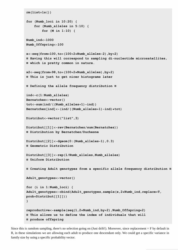
rmlistlsfor Numbloci in 10:20

for Numballeles in 5:10 for M in 1:10

Numbind1000NumbOffspring100

xseqfrom100,to1002Numballeles2,by2 Having this will correspond to sampling dinucleotide microsatellites, which is pretty common in nature.

x2seqfrom98,to1002Numballeles,by2 This is just to get nicer histograms later

Defining the allele frequency distribution

indc1:NumballelesBernatchezvectortotsumindNumballeles1indBernatchezindindNumballeles1indtotDistributvector"list",3Distribut1revBernatchezsumBernatchez Distribution by BernatchezDuchesneDistribut2dgeom0:Numballeles1,0.3 Geometric Distribution

Distribut3rep1Numballeles,Numballeles Uniform Distribution

Creating Adult genotypes from a specific allele frequency distribution

Adultgenotypesvectorfor i in 1:Numbloci AdultgenotypescbindAdultgenotypes,samplex,2Numbind,replaceT,probDistribut1reproductivesampleseq1,2Numbind,by2,NumbOffspring2 This allows us to define the index of individuals that will produce offspring

Since this is ramdom sampling, there's no selection going on (Just drift!). Moreover, since replacement = F by default inR, in these simulations we are allowing each adult to produce one descendant only. We could get a specific variance infamily size by using a specific probability vector.



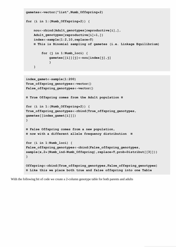
gametesvector"list",NumbOffspring2for i in 1:NumbOffspring2

nourbindAdultgenotypesreproductivei,,Adultgenotypesreproductivei1,indexsample1:2,10,replaceT This is Binomial sampling of gametes i.e. Linkage Equilibrium

for j in 1:Numbloci gametesijnouindexj,j

indexgametsample1:200TrueoffspringgenotypesvectorFalseoffspringgenotypesvector True Offspring comes from the Adult population

for i in 1:NumbOffspring2 TrueoffspringgenotypesrbindTrueoffspringgenotypes,gametesindexgameti False Offspring comes from a new population, now with a different allele frequency distribution

for i in 1:Numbloci FalseoffspringgenotypescbindFalseoffspringgenotypes,samplex,2NumbindNumbOffspring,replaceT,probDistribut3OffspringrbindTrueoffspringgenotypes,Falseoffspringgenotypes Like this we place both true and false offspring into one Table

With the following bit of code we create a 2-column genotype table for both parents and adults



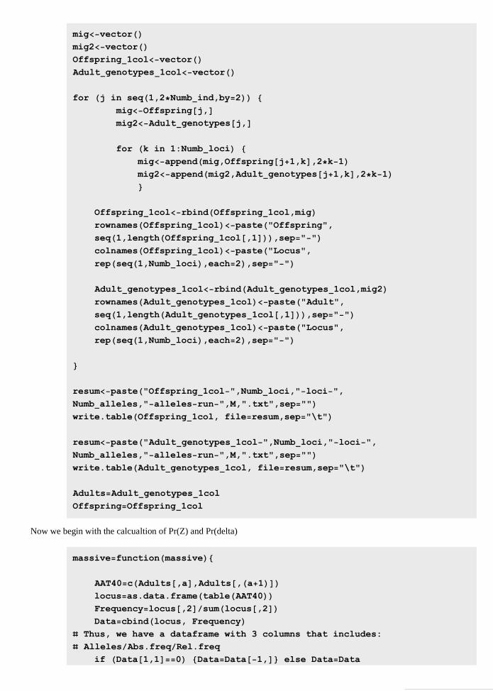
migvectormig2vectorOffspring1colvectorAdultgenotypes1colvectorfor j in seq1,2Numbind,by2

migOffspringj,mig2Adultgenotypesj,for k in 1:Numbloci

migappendmig,Offspringj1,k,2k1mig2appendmig2,Adultgenotypesj1,k,2k1

Offspring1colrbindOffspring1col,migrownamesOffspring1colpaste"Offspring",seq1,lengthOffspring1col,1,sep""colnamesOffspring1colpaste"Locus",repseq1,Numbloci,each2,sep""Adultgenotypes1colrbindAdultgenotypes1col,mig2rownamesAdultgenotypes1colpaste"Adult",seq1,lengthAdultgenotypes1col,1,sep""colnamesAdultgenotypes1colpaste"Locus",repseq1,Numbloci,each2,sep""

resumpaste"Offspring1col",Numbloci,"loci",Numballeles,"allelesrun",M,".txt",sep""write.tableOffspring1col, fileresum,sep"\t"resumpaste"Adultgenotypes1col",Numbloci,"loci",Numballeles,"allelesrun",M,".txt",sep""write.tableAdultgenotypes1col, fileresum,sep"\t"AdultsAdultgenotypes1colOffspringOffspring1col

Now we begin with the calcualtion of Pr(Z) and Pr(delta)

massivefunctionmassiveAAT40cAdults,a,Adults,a1locusas.data.frametableAAT40Frequencylocus,2sumlocus,2Datacbindlocus, Frequency

Thus, we have a dataframe with 3 columns that includes: AllelesAbs.freqRel.freq

if Data1,10 DataData1, else DataData



In case there's null allele 0n1lengthAAT402

Total number of individuals sampled assuming diploidy

A1Data,32n1A2Data,3^2n1AAA1A2AAAcbindData,AA

Thus, we're adding a column that includes the 2zz2 Now we do exactly the same for the offspring

AAT402cOffspring,a,Offspring,a1locus2as.data.frametableAAT402Frequency2locus2,2sumlocus2,2Data2cbindlocus2, Frequency2if Data21,10 Data2Data21, else Data2Data2n2lengthAAT4022B1Data2,32n2B2Data2,3^2n2BBB1B2BBBcbindData2,BB

Now we focus on the alleles that are found both in the parentals and in the offspring. It is important to note that alleles occurring in only one sample i.e. adults or juveniles will not be included in the calculation because the product equals zero.

AAA1matchBBB,1,AAA,1gwhichAAA10g1AAA1gAAA1AAAg1,BBB1matchAAA,1,BBB,1jwhichBBB10j1BBB1jBBB1BBBj1,

So we take the product and sum it

ABAAA1,4BBB1,4ABsumAB

Now we make two columns with the different allele combinations and get rid of the 'homozygotes' using the line: whichAgenotypes,1Agenotypes,2. Please, notice that now we are dealing with the shared alleles from parents AAA1 and offspring BB1

yAAA1,1



Agenotypesexpand.gridy,yremove2whichAgenotypes,1Agenotypes,2AgenotypesAgenotypesremove2,zBBB1,1Bgenotypesexpand.gridz,zremove2whichBgenotypes,1Bgenotypes,2BgenotypesBgenotypesremove2,

This allows us to calculate the genotype frequencies in Adults and Offspring

onematchAgenotypes,1,AAA1,1twomatchAgenotypes,2,AAA1,1oneAAA1one,3

Like this we get a vector that includes allele frequencies instead of allele names

twoAAA1two,3 Like this we get a vector that includes allele frequencies instead of allele names, but for the second column

Agfreqonetwon12

onebmatchBgenotypes,1,BBB1,1twobmatchBgenotypes,2,BBB1,1onebBBB1oneb,3twobBBB1twob,3Ogfreqonebtwobn22

GfreqsAgfreqOgfreqGfreqsfloorGfreqsGfreqsumGfreqs2PrBABGfreqn1n2

So this is the probability of a randomly selected dyad from a particular locus sharing an allele

nompaste"PrZ",Numbloci,"loci",Numballeles,"allelesrun",M,".txt",sep""write.tablePrB,filenom,row.namesFALSE,col.namesF,sep"\t",appendT

alncolAdultsC1fora in seq1,al,2 lapplya,massivenompaste"PrZ",Numbloci,"loci",

Numballeles,"allelesrun",M,".txt",sep""PrBs read.tablenom, headerF, sep"\t",

na.strings"NA", dec".", strip.whiteTRUE



nn1lengthAdults,1nn2lengthOffspring,1Prdelta prodPrBs,1ExpectedNumberofFalsePairs Prdeltann1nn2pvalue1cbindExpectedNumberofFalsePairs,Prdeltanom2paste"FpairsPrdelta",Numbloci,"loci",

Numballeles,"alleles.txt",sep""write.tablepvalue1,filenom2,row.namesFALSE,sep"\t",appendT

Begin dyad sorting. Note that allele sizes must be the same order of magnitude

AnamesrownamesAdultgenotypes1colOnamesrownamesOffspring1colcategoriesncolAdultsAindividslengthAdults,1OindividslengthOffspring,1A1:AindividsO1:OindividsGexpand.gridA,OAGG,1AOG,2AdsAdultsAG,OffsOffspringAO,IdnamesAAnamesAGIdnamesOOnamesAOwrite.tableIdnamesA,file"IdnamesA.txt",

row.namesFALSE,col.namesF,sep"\t",appendFwrite.tableIdnamesO,file"IdnamesO.txt",

row.namesFALSE,col.namesF,sep"\t",appendFIdnamesAread.table"IdnamesA.txt",headerF,

sep"\t",na.strings"NA",dec".",strip.whiteTRUEIdnamesOread.table"IdnamesO.txt",headerF,

sep"\t",na.strings"NA",dec".",strip.whiteTRUENamescbindIdnamesA,IdnamesOmatchesfunctionmatches AAds,zOffs,zBAds,z1Offs,z1CAds,zOffs,z1DAds,z1Offs,zfABCDff^2fcbindz,f



write.tablef,file"Sort.txt",row.namesFALSE,col.namesF,sep"\t",appendTzncolAdsC1forz in 2uniqueround1:z221 lapplyz,matchesObservedread.table"Sort.txt",headerF,sep"\t",

na.strings"NA",dec".",strip.whiteTRUEauniqueObserved,1UNULL

for i in a uObservedObserved,1i,2 UcbindU,ualengthU,1stuffrowSumsUSortedcbindNames,stuffmatcheswhichSorted,30ActualsortstuffIDSwhichstuff0PAdultsAdsIDS,POffspringOffsIDS,nputlengthmatchesPutativepairsSortedmatches,PhiExpectedNumberofFalsePairsnputif Phi1 Phi1Phicbind"Phi",Phinom3paste"Phi",Numbloci,"locirun",M,".txt",sep""write.tablePhi,filenom3,row.namesFALSE,col.namesF,sep"\t",appendTunlink"Sort.txt"unlink"IdnamesA.txt"unlink"IdnamesO.txt"

This will end the exclusion probability calculations

Using a Mathematica notebookMathematica has a front end and a kernel, which work independently: one handles formatting, the other the calculations.If the kernel crashes, the calculations are lost; if the front end crashes, the current notebook is lost. Save regularly!



To find out about a function, use ?name, and then type [enter]. For example:

? IterateCline

Information::notfound: Symbol IterateCline not found.

This also works for inbuilt functions. You can find out more about them using the Help... menu; packages aredocumented under Add-Ons.

Cells are structured by headings, subheadings etc. Double click on the right-hand brackets to open & close them.

To find out where do you have to install your add-ons or where is your Base Directory you type:

$UserBaseDirectory This is where you have your Mathematica packagesC:\Documents and Settings\Phyllamphion\Datos de programa\Mathematica

To find out where does Mathematica send the files containing the genotypes from simulated individuals you type:

Directory This is where the files are going toC:\Documents and Settings\Phyllamphion\Mis documentos

