FEP WORKING PAPERS Research Work in FEP WORKING … · percentoftheindustriesthespatialbreakdownhas10orlessareas.2 Beyond thispracticalconstraint,Adelman’s(1955)indexofﬁrmverticaldisintegra

Vertical Disintegration in Vertical Disintegration in MarshallianMarshallian Industrial DistrictsIndustrial Districts

Octávio Figueiredo*Paulo Guimarães**

Douglas Woodward***

*Universidade do Porto and CEMPRE

**University of South Carolina and CEMPRE

***University of South Carolina

FEP WORKING PAPERSFEP WORKING PAPERS ResearchWork in

ProgressFEP WORKING PAPERSFEP WORKING PAPERSn. 280, June 2008

Vertical Disintegration in Marshallian

Industrial Districts1

Octávio Figueiredo

Universidade do Porto and CEMPRE

Paulo Guimarães

University of South Carolina and CEMPRE

Douglas Woodward

University of South Carolina

June 19, 2008

1The authors acknowledge the support of FCT, the Portuguese Foundation

for Science and Technology. We thank the Ministry of Employment, Statistics

Department, for the permission to use the Quadros do Pessoal database.

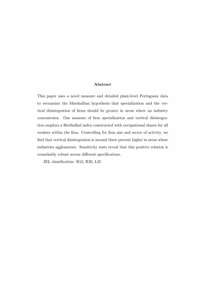
Abstract

This paper uses a novel measure and detailed plant-level Portuguese data

to reexamine the Marshallian hypothesis that specialization and the ver-

tical disintegration of firms should be greater in areas where an industry

concentrates. Our measure of firm specialization and vertical disintegra-

tion employs a Herfindhal index constructed with occupational shares for all

workers within the firm. Controlling for firm size and sector of activity, we

find that vertical disintegration is around three percent higher in areas where

industries agglomerate. Sensitivity tests reveal that this positive relation is

remarkably robust across different specifications.

JEL classification: R12, R39, L25

1 Introduction

How does the scale of production at a location affect the organization of

production at this location? Interest in this central question dates back to

Smith (1776) who asserted that occupational specialization (or the division

of labor) within the firm is "limited by the extent of the market."1 In his

celebrated 1890 text, Principles of Economics, Alfred Marshall advanced

a related theorem about industrial concentration across space, suggesting

that firm specialization and vertical disintegration should be greater in areas

where an industry concentrates:

When an industry has thus chosen a locality for itself, it is

likely to stay there long: so great are the advantages which people

following the same skilled trade get from near neighbourhood to

one another. [...] And presently subsidiary trades grow up in

the neighbourhood, supplying it with implements and materials,

organizing its traffic, and in many ways conducing to the economy

of its material [Marshall (1890), book IV, chapter X].

1Recall the well-known example of the division of labor in pin manufacture with which

Adam Smith opens The Wealth of Nations. When pin manufacture is in a primitive stage

of development the whole and undivided process of production of a pin within the firm is

carried out by one person. With increases in the extent of markets, however, it becomes

increasingly feasible to divide the labor of pin making into a sequence of specialized tasks

attended to by detailed workers within the firm. Thus, a transformation of pin making

firms comes about, and the labor process is fragmented into several activities, such as

drawing, straightening, cutting, pointing, grinding, head-making, whitening, and so on.

With increasing volume of output, the division of labor within the firm tends to become

increasingly more finely grained.

1

Marshall’s notion that industrial localization would engender vertical dis-

integration and spur the emergence of a wide variety of specialized suppliers

in the area infuses a large body of theorethical work, from the "new eco-

nomic geography" to modern theories of growth and international trade [see

for example Rivera-Batiz (1988), Krugman (1991), Arthur (1994), Venables

(1996), Rodríguez-Clare (1996) and Hanson (1996)]. This theorethical re-

search emphasizes the importance of industry-specific external economies.

Less progress has been made in the empirical verification of the Mar-

shallian hypothesis. Within the literature on industrial districts, many case

studies illustrate the presence of specialized suppliers and firm vertical dis-

integration in particular areas and industries [for surveys see Piore & Sabel

(1984) and Markusen (1996)]. Yet, the issue of whether these cases have

wider relevance remains an open empirical question.

As noted by Rosenthal & Strange (2004), Holmes (1999) represents the

only systematic statistical study addressing the Marshallian hypothesis to

date. The author found a positive correlation between localization of an

industry and firm vertical disintegration for the U.S. manufacturing sector.

To measure localization, Holmes (1999) used 1987 employment data at the

establishment level. Vertical disintegration was measured using a Purchased

Input Intensity (PII) index (the ratio of purchased inputs to output), a mea-

sure derived from Adelman’s (1955) index of firm vertical disintegration. Yet,

the lack of establishment level data for the PII index forced the author to

aggregate up the employment data set. The spatial level of aggregation for

the 459 industries used in his study varies considerably. For more than 50

2

percent of the industries the spatial breakdown has 10 or less areas.2 Beyond

this practical constraint, Adelman’s (1955) index of firm vertical disintegra-

tion has significant theoretical limitations. Above all, the index is sensitive

to the stage of the production process. The earlier disintegration occurs in

the process, the less sensitive the index becomes to changes in the degree of

firm integration.

In this paper we use a novel measure and establishment- (plant-) level

Portuguese data to evaluate the proposition that the vertical disintegration

of firms should be greater in areas where an industry concentrates. Our

approach addresses the essential problem associated with Holmes’s (1999)

empirical analysis. First, because we have access to detailed establishment

data for all regions and industries, we are able to use the plant as the unit

of observation. We also know the occupation of every employee in each

establishment. This allows us to compute an alternative, improved measure

of vertical disintegration based on the occupational specialization within the

establishment. Applied to Portuguese data, after controlling for firm size

and sector, we find that firms’ vertical disintegration is about three percent

higher in areas where industries agglomerate.

In the next section we review measures of firm vertical disintegration and

motivate our approach to accounting for firm specialization. In section 3,

we discuss the measurement of localization of an industry. Section 4 present

our main findings and implements several sensitivity tests, while section 5

concludes the paper.

2Holmes (1999) notes that these areas can be counties, metropolitan statistical areas,

states, or even larger units. For example, the creamery butter industry is partitioned into

only two areas: the state of Wisconsin and the rest of the United States.

3

2 Measuring Vertical Disintegration

The most commonly used measure of firm vertical disintegration is Adelman’s

(1955) index: the ratio of value added to sales [see Davies & Morris (1995)

for a survey]. Limitations of this measure, however, have been pointed out

over the years by Barnes (1955), Eckard (1979) and Maddigan (1981). The

main problem is the sensitivity to the stage of the production process, well

illustrated in Holmes (1999). Consider the following scenario. There are three

firms, each one undertaking one of the three stages of a sequential production

process. Additionally, suppose that all firms contribute the same amount of

added value to the final product. Now, even though all the three firms are

vertically integrated to the same extent, because sales increase as we move

along the production chain, Adelman’s (1955) index will result in a series of

decreasing values. Another problem when implementing this measure is the

dearth of adequate micro-level data sets. In most countries and regions, data

on the value of inter-firm transactions are not available.

In this paper we take a different tack and construct an internal measure

of firm vertical disintegration. The analysis is based on a comprehensive

Portuguese manufacturing employer-employee data set, the Quadros do Pes-

soal.3 The data set includes the universe of all plants in Portugal, with precise

information on plant location, firm start-up date, sector of activity, actual

employment, and characteristics of the workforce. Of particular interest is

information on the occupation of entire workforce for each firm. Every worker

is coded using the Portuguese National Classification of Occupations (CNP),

3This survey collects information for all the establishments operating in Portugal, ex-

cept family businesses without wage-earning employees.

4

which follows the current International Standard Classification of Occupa-

tions (ISCO).4 This allows us to construct an establishment-level measure

of vertical integration based on occupational specialization within the es-

tablishment. If we compare two equally sized establishments in the same

industry we would expect the establishment that undertakes more stages of

production (the more integrated) to have a larger and more diversified mix

of occupations.

In turn, to measure establishment vertical disintegration we propose a

Herfindhal index constructed with the shares of workers on each occupation.

That is,

Hi =

Zi∑

z=1

(xzixi

)2, (1)

where xzi denotes establishment’s i employment in occupation z, xi stands

for total employment in establishment i, and Zi is establishment’s i total

number of occupations.

To get some insight about the validity of our proposed measure we can

apply this same logic to manufacturing sectors as a whole. Because subsec-

tors tend to correspond to different production stages of sectors, if a cor-

respondence exists between the occupations and the different phases of the

productive process, then we would expect an increase in the Herfindhal index

of occupations (calculated at the industry level) as we move from a broader

to a finer definition of an industry. Table 1 shows the results of such exercise,

by computing average Herfindhal indexes for different levels of aggregation of

4The ISCO is a tool for organizing jobs into a clearly defined set of groups according

to the tasks and duties undertaken in the job.

5

the manufacturing sectors. Information is for the year of 2005, the most re-

cent available year in our data set. We make use of the Portuguese Standard

Industrial Classification system (CAE rev.2) at the 2-digit (22 industries),

3-digit (100 industries) and 5-digit (315 industries) levels.5 Occupations are

coded according to the Portuguese CNP at 6-digits, the more detailed level

of disaggregation. At this level, we have 1,751 different occupations in the

manufacturing sector as a whole for the year of 2005.

[insert Table 1 about here]

As can be seen in Table 1, the Herfindhal measure behaves as expected

when we move from a broader to a finer definition of industries. Yet, com-

paring the Herfindhal in this manner can be misleading because the average

gives equal importance to all sectors within each level of CAE rev.2. Hence,

we also compared the Herfindhal of each subindustry with its parent in the

industry.6 We found that 81 of the 98 3-digit Herfindhal indexes for which

the CAE rev.2 distinguish the 2 from the 3-digit levels are larger than their

2-digit counterparts (83 percent) and that these numbers are 246 out of 284

(87 percent) for the 5 versus 3-digit comparison.

It may be argued that these results are driven by chance. To address this

concern, we implemented a simple permutation test. The test builds on the

idea that if the mix of occupations is the same in the sector and the subsectors

then differences in Herfindhals should be attributed to chance alone. Hence,

5These are the numbers of industries we observe for this particular year.6It should be noted here that for 2 industries the Portuguese Standard Industrial Clas-

sification system (CAE rev.2) does not distinguish the 3 from the 2-digit levels. The same

occurs for 31 industries when we move from 5 to 3-digit. In these cases, by definition, the

Herfindhal for the industry is identical to that of the subindustry.

6

to test this hypothesis, for each sector we randomly rearranged the assign-

ment of existing occupations to workers. This procedure was implemented

1,000 times and the Herfindhal indexes for each subsector were calculated in

each permutation of the data. Comparison of the actual Herfindhal values

for the subsectors with those obtained by permutation allow us to infer the

likelihood of obtaining a value as extreme (as high) as the one actually ob-

served. Thus, we perform a one-sided test of hypothesis using as reference

the empirical distribution of the Herfindhals obtained by the procedure de-

scribed above. For 93 percent of the 81 3-digit industries for which the actual

3-digit Herfindhal indexes are larger than their 2-digit counterparts we reject

the hypothesis at a 95 percent level of significance and the corresponding

percentage for the 246 5-digit industries is 86 percent.

This industry-level analysis lends credibility to the idea that occupation

data can be used to measure vertical disintegration. We now turn to the

measurement of industry concentration, or localization.

3 Measuring Localization

Typically, measures of industry localization are based on employment. Some

authors [such as Holmes (1999) andWheeler (2006)] have used aggregate local

employment while others calculate location quotients [see for example Kim

(1995) and Holmes & Stevens (2002)]. These quotients summarize the extent

to which industries are disproportionately represented in total employment

(relative to the national level) across a collection of regions.

As argued in Figueiredo, Guimarães & Woodward (2007) the use of em-

ployment based indexes to measure localization is questionable. These mea-

7

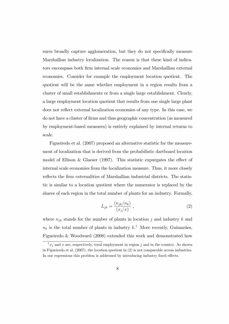
sures broadly capture agglomeration, but they do not specifically measure

Marshallian industry localization. The reason is that these kind of indica-

tors encompass both firm internal scale economies and Marshallian external

economies. Consider for example the employment location quotient. The

quotient will be the same whether employment in a region results from a

cluster of small establishments or from a single large establishment. Clearly,

a large employment location quotient that results from one single large plant

does not reflect external localization economies of any type. In this case, we

do not have a cluster of firms and thus geographic concentration (as measured

by employment-based measures) is entirely explained by internal returns to

scale.

Figueiredo et al. (2007) proposed an alternative statistic for the measure-

ment of localization that is derived from the probabilistic dartboard location

model of Ellison & Glaeser (1997). This statistic expurgates the effect of

internal scale economies from the localization measure. Thus, it more closely

reflects the firm externalities of Marshallian industrial districts. The statis-

tic is similar to a location quotient where the numerator is replaced by the

shares of each region in the total number of plants for an industry. Formally,

Ljk =(njk/nk)

(xj/x), (2)

where njk stands for the number of plants in location j and industry k and

nk is the total number of plants in industry k.7 More recently, Guimarães,

Figueiredo & Woodward (2008) extended this work and demonstrated how

7xj and x are, respectively, total employment in region j and in the country. As shown

in Figueiredo et al. (2007), the location quotient in (2) is not comparable across industries.

In our regressions this problem is addressed by introducing industry fixed effects.

8

the framework of Ellison & Glaeser (1997) can also be used to derive statis-

tical tests for the measure in (2).8

We are interested in testing whether firms inside areas of localization

of an industry are more vertically disintegrated than more isolated firms.

Therefore, in our empirical analysis, the identification of areas of localization

is implemented by dichotomizing the location quotient between values above

and below one.9 To obviate the problem of having the own plant contribut-

ing to both sides of the regression we excluded the current plant from the

calculation of the localization measure.10 We calculate localization measures

using the Portuguese concelho as the spatial unit of analysis.11 Industries

are classified according to the 3-digit (103 industries) classification of the

Portuguese Standard Industrial Classification system (CAE rev.2).

8Later, in the empirical analysis, we will use the statistic,

Wjk =J [log(Ljk)]

2

(J − 2)n−1jk + nk,

to check whether the plant counts based location quotient in (2) provides evidence of

localization in excess of what would be expected to arise randomly. In the above formula

nk is the mean of all n−1jk for industry k. The statistic is asymptotically distributed as

chi-square with one degree of freedom.9In addition to this localization dummy variable, later on, as part of our sensitivity

tests, we will also use the location quotient directly in the regression as in Holmes (1999).10That is, we computed the following plant count location quotient to construct the

dummy variable that enters in our regressions:

Lijk =(njk − 1)/(nk − 1)

(xj − xi)/(x− xi)) .

11We restrict analysis to continental Portugal. The concelho is a Portuguese adminis-

trative region roughly equivalent to the U.S. county. In continental Portugal there are 278

concelhos with an average area of 320.3 square kilometers.

9

4 Empirical Results

4.1 Main Results

Table 2 presents our main results. The dependent variable is the logarithm

of the establishment-level Herfindhal index in (1) and the localization vari-

able is the dummy variable described above. We used panel data for the

period 2002-2005.12 Besides fixed effects for industry and year, in column

(1), we also introduced a fixed effect for establishment size. This was done

mainly because the range of variation of the Herfhindhal is constrained by

the size of the establishment.13 The models were estimated by ordinary least

squares with a correction for the standard errors. This correction accounts

for possible unobservable correlation between repeated observations (i.e., the

same establishment in different years) and produces rather conservative t-

statistics.14

The use of fixed effects for establishment size is desirable because it does

not impose a functional structure in the relation. However, it has the adverse

effect of removing all the singleton observations, a problem more likely to

affect large establishments. Thus, we also ran the regression in column (2)

of Table 1 where we include size directly as a regressor.

Both regressions produce similar results. As can be seen, controlling

12We choose this particular period of time because the Quadros do Pessoal data set

does not report worker level data for the year of 2001. Another reason is that in 1999 the

number of concelhos has been changed in continental Portugal.13We also excluded from the regressions establishment with only one employee because

in that case the Herfindhal is constrained to 1.14We use cluster-robust standard errors [see Cameron & Trivedi (2005)]. In our appli-

cation, this generates more conservative estimates than conventional heteroskedasticity-

robust (White) standard errors.

10

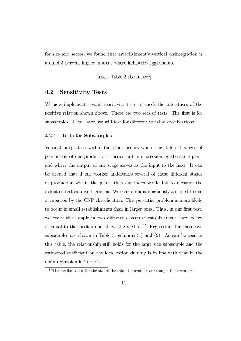
for size and sector, we found that establishment’s vertical disintegration is

around 3 percent higher in areas where industries agglomerate.


4.2 Sensitivity Tests

We now implement several sensitivity tests to check the robustness of the

positive relation shown above. There are two sets of tests. The first is for

subsamples. Then, later, we will test for different variable specifications.

4.2.1 Tests for Subsamples

Vertical integration within the plant occurs where the different stages of

production of one product are carried out in succession by the same plant

and where the output of one stage serves as the input to the next. It can

be argued that if one worker undertakes several of these different stages

of production within the plant, then our index would fail to measure the

extent of vertical disintegration. Workers are unambiguously assigned to one

occupation by the CNP classification. This potential problem is more likely

to occur in small establishments than in larger ones. Thus, in our first test,

we broke the sample in two different classes of establishment size: below

or equal to the median and above the median.15 Regressions for these two

subsamples are shown in Table 3, columns (1) and (2). As can be seen in

this table, the relationship still holds for the large size subsample and the

estimated coefficient on the localization dummy is in line with that in the

main regression in Table 2.

15The median value for the size of the establishments in our sample is six workers.

11


Another potential drawback of our analysis is that younger firms may

have not reached their optimal structure of occupations and this may bias

the results. Ono (2003) puts forward the argument that firms need time

to develop their ties with business partners and find their optimal matches.

Thus, our second test separates establishments according to their firm’s age.

Columns (3) and (4) of Table 3 show that the relationship holds for both

establishments pertaining to the younger firms (with an age below or equal

to the median) and to more mature firms (above median age).16 Again, the

estimated coefficients on the localization dummy are in line with that in the

main regression in Table 2.

As in Holmes (1999), we also split our sample according to the Ellison

& Glaeser’s (1997) index.17 In Table 3, column (5), we show regressions

for the industries in the top half of the Ellison & Glaeser’s (1997) measure.

Results for the other half, the least geographically concentrated industries,

are in column (6).18 We obtain estimates in line with Holmes (1999). For the

most concentrated industries, the coefficient is much larger than in the main

regression in Table 2, and it goes to zero for the least concentrated ones. As

argued by Holmes (1999), this pattern provides some evidence that increased

opportunity for vertical disintegration may be a factor that explains why

some industries concentrate in space. Establishments in dispersed industries

16The median age for the firms in our sample is eleven years.17For the reason discussed in section 3, we computed the Ellison & Glaeser’s (1997) index

using counts of plants instead of employment. This count based version of the Ellison &

Glaeser’s (1997) index is discussed in Guimarães, Figueiredo & Woodward (2007).18The concentration measure has been calculated using data for the year of 2005.

12

do not specialize even when they locate in areas of agglomeration of their

industry.

4.2.2 Tests for Different Variable Definitions

In this subsection we test the robustness of the relationship by employing

alternative definitions for the main right and left-hand side variables in the

regression. To start with, we checked whether changes in the definition of

the right-hand side variable affected our main results. In the first test [Table

4, column (1)], we used the 5-digit (325 industries) classification of the Por-

tuguese Standard Industrial Classification system (CAE rev.2) to calculate

the location quotient. This regression allows us to test if the relation still

holds when we use a finer classification of industries. Then, in Column (2),

we implemented a second experiment by making use of the statistical test

discussed earlier to define our localization dummy variable. Now, instead

of dichotomizing the location quotient above and below unity, we coded the

variable as one only when the quotient passed the one-sided test at the 95

percent level of significance. This statistical test allows for a stricter def-

inition of areas of localization because it accounts for spurious geographic

concentration (that is, concentration that occurs by chance alone). Finally,

in Table 4, column (3), we make a third experiment by entering the loga-

rithm of the plant count location quotient directly as a regressor instead of

the localization dummy variable.19

We also performed similar robustness checks for the left-hand side vari-

19A continuous employment quotient as in Holmes & Stevens (2002) was also tried.

Results are not reported because they are very similar to those obtained with the plant

count continuous version shown in Table 4.

13

able. As indicated before, our measure of vertical disintegration relies on

the 6-digit level of the Portuguese National Classification of Occupations

(CNP). Because the Quadros do Pessoal data set is collected by means of

a self-reported questionnaire it may be argued that with the 6-digit clas-

sification system for occupations there is more room for coding errors and

ambiguities. If that were the case, the Herfindhal index could reflect more

variability than that implied by the actual division of labor within the es-

tablishment. To check if this potential problem is biasing our results, in the

regression in column (5) of Table 4, we computed the Herfindhal index using

the 3-digit level of the CNP (116 job groups) instead of the 6-digit (1,891

groups) used so far.20 At this coarser level of aggregation we loose precision

but room for coding errors and ambiguities is smaller.

A criticism leveled by Eckard (1979) to establishment-based measures of

vertical disintegration is that they ignore multiplant firms. In this case, verti-

cal disintegration may occur within a firm but across establishments. Again,

this situation results in measurement error that could bias our estimates.

Accounting for this type of disintegration requires information linking estab-

lishments with firms. Because we have this information, in the last column

of Table 4 we used the logarithm of a Herfindhal at the firm level as our

left-hand side variable.21


As can be seen in Table 4, the positive relationship between vertical disin-

20These are the numbers of occupations groups in the manufacturing sector we observe

for the 2002-2005 period.21All establishments of a firm were lumped together if they belonged to the same industry

and were located in the same concelho.

14

tegration and localization of an industry still holds across specifications. The

magnitude of the coefficients for the localization variable and the quality of

the adjustment are also quite similar for the different specifications. The only

exception is the regression that employs a coarser definition of occupations.

In that case, the estimated coefficient is slightly higher but the quality of the

adjustment falls considerably. Note also that the coefficient of the regression

with the continuous location quotient is not comparable with the others.

5 Conclusion

Marshall’s hypothesis that industry localization would prompt vertical dis-

integration and the emergence of specialized suppliers underlies a large body

of recent theorethical work, from the "new economic geography" to mod-

ern theories of growth and international trade. These studies emphasize the

importance of industry-specific external economies.

Less research has been done regarding the empirical verification of Mar-

shall’s central claim. Case studies of industrial districts often point to the

presence of specialized suppliers and vertical disintegration of firms in partic-

ular areas. Yet rigorous statistical research is rare. Thus far, Holmes (1999)

remains the only systematic empirical study to address the question.

Our paper posits a new measure of vertical disintegration and tests it

against plant-level Portuguese data. The results provide evidence supporting

Marshall’s suggestion that vertical disintegration of firms should be greater

in areas where an industry concentrates. Controlling for firm size and sector

of activity, we found that firm vertical disintegration is around three per-

cent higher in areas where industries agglomerate. Various sensitivity tests

15

indicate that this positive relation is remarkably robust across specifications.

In an original approach, we develop an internal occupational measure of

firm disintegration. This measure is a Herfindhal index constructed with

the shares of workers on each occupation within the firm. It overcomes the

long-standing problem associated with Adelman’s (1955) measure of firm

vertical disintegration: The earlier disintegration occurs in the production

process the less sensitive the measure becomes to changes in the degree of

firm integration. Indeed, there is no reason to believe that our index is sen-

sitive to the stage of the production process. Moreover, because our measure

is constructed with data on workers’ occupations, increased availability of

employer-employee data sets with spatial information should allow the ex-

tension of our approach to other countries and regions.

16

References

Adelman, M. A. (1955), Concept and statistical measurement of vertical

integration, in G. J. Stigler, ed., ‘Business Concentration and Price

Policy’, Princeton University Press, Princeton, NJ, pp. 281—322.

Arthur, W. B. (1994), Increasing Returns and Path Dependence in the Econ-

omy, University of Michigan Press, Ann Arbor, MI.

Barnes, I. R. (1955), Comment, in G. J. Stigler, ed., ‘Business Concentration

and Price Policy’, Princeton University Press, Princeton, NJ, pp. 322—

330.

Cameron, A. C. & Trivedi, P. K. (2005), Microeconometrics: methods and

applications, Cambridge University Press, Cambridge, NY.

Davies, S. & Morris, C. (1995), ‘A new index of vertical integration: Some

estimates for UK manufacturing’, International Journal of Industrial

Organization 13(2), 151—177.

Eckard, E. W. (1979), ‘A note on the empirical measurement of vertical

integration’, Journal of Industrial Economics 28(1), 105—107.

Ellison, G. & Glaeser, E. (1997), ‘Geographic concentration in U.S. manufac-

turing industries: A dartboard approach’, Journal of Political Economy

105(5), 889—927.

Figueiredo, O., Guimarães, P. & Woodward, D. (2007), Localization

economies and establishment scale: A dartboard approach. FEP Work-

ing Paper, n.247.

17

Guimarães, P., Figueiredo, O. & Woodward, D. (2007), ‘Measuring the lo-

calization of economic activity: A parametric approach’, Journal of Re-

gional Science 47(4), 753—774.

Guimarães, P., Figueiredo, O. & Woodward, D. (2008), Dartboard tests for

the location quotient. FEP Working Paper, n.273.

Hanson, G. H. (1996), ‘Localization economies, vertical organization, and

trade’, American Economic Review 86(5), 1266—1278.

Holmes, T. (1999), ‘Localization of industry and vertical disintegration’, The

Review of Economics and Statistics 81(2), 314—325.

Holmes, T. & Stevens, J. (2002), ‘Geographic concentration and establish-

ment scale’, The Review of Economics and Statistics 84(4), 682—690.

Kim, S. (1995), ‘Expansion of markets and the geographic distribution of

economic activities: the trends in U.S. regional manufacturing structure,

1860-1987’, Quarterly Journal of Economics 110(4), 881—908.

Krugman, P. (1991), ‘Increasing returns and economic geography’, Journal

of Political Economy 99(3), 483—499.

Maddigan, R. (1981), ‘The measurement of vertical integration’, The Review

of Economics and Statistics 63(3), 328—335.

Markusen, A. (1996), ‘Sticky places in slippery space: A typology of indus-

trial districts’, Economic Geography 72(3), 293—313.

Marshall, A. (1890), Principles of Economics, Macmillan. Eighth edition,

1920, London.

18

Ono, Y. (2003), ‘Outsourcing business services and the role of central admin-

istrative offices’, Journal of Urban Economics 53(3), 377—395.

Piore, M. J. & Sabel, C. F. (1984), The Second Industrial Divide, Basic

Books, New York.

Rivera-Batiz, F. L. (1988), ‘Increasing returns, monopolistic competition,

and agglomeration in consumption and production’, Regional Science

and Urban Economics 18(1), 125—153.

Rodríguez-Clare, A. (1996), ‘Multinationals, linkages, and economic devel-

opment’, American Economic Review 88(4), 852—873.

Rosenthal, S. & Strange, W. (2004), Evidence on the nature and sources

of agglomeration economies, in J. V. Henderson & J. F. Thisse, eds,

‘Handbook of Regional and Urban Economics’, Elsevier, Amsterdam,

pp. 2119—2171.

Smith, A. (1776), An Inquiry into the Nature and Causes of the Wealth of

Nations, Methuen. Fifth edition, 1904, London.

Venables, A. (1996), ‘Localization of industry and trade performance’, Oxford

Review of Economic Policy 12(3), 52—60.

Wheeler, C. H. (2006), ‘Productivity and the geographic concentration of in-

dustry: The role of plant scale’, Regional Science and Urban Economics

36(3), 313—330.

19

Table1:AverageHerfindhalIndexAcrossSectors

CAErev.2

2-digit

3-digit

5-digit

HerfindhalIndex

6.3%

6.8%

9.1%

NumberofSectors

22100

315

20

Table2:RegressionEstimates

(1)

(2)

LocalizationDummy

0.030(7.7)

0.029(7.2)

LogofSize

--0.311(-133.1)

FixedEffects

Size

Yes

No

Industry

Yes

Yes

Year

Yes

Yes

R2

42,0%

39.7%

N167,921

167,921

Note:t-statisticsassociatedwithcluster-robuststandarderrorsinparenthesis.

21

Table3:RegressionEstimatesforSubsamples

ClassesofSize

ClassesofAge

MostversusLeast

ConcentratedIndustries

(1)Small

(2)Large

(3)Young

(4)Old

(5)Most

(6)Least

LocalizationDummy

0.024(5.7)

0.030(4.4)

0.031(6.2)

0.028(4.6)

0.047(7.9)

0.009(1.6)

LogofSize

-0.482(-103.2)

-0.237(-53.0)-0.278(-82.5)-0.326(-103.1)

-0.293(-101.9)

-0.341(-87.5)

FixedEffects

Industry

Yes

Yes

Yes

Yes

Yes

Yes

Year

Yes

Yes

Yes

Yes

Yes

Yes

R2

24.4%

28.4%

30.8%

43.1%

39.4%

40.5%

N84,641

83,280

86,345

81,576

93,706

74,215

Note:t-statisticsassociatedwithcluster-robuststandarderrorsinparenthesis.

22

Table4:RegressionEstimatesforDifferentVariableDefinitions

(1)5-digit

(2)Statistically

(3)Continuous(4)3-digit

(5)Herfindhal

Industry

Significant

Location

Occupations

ForFirms

Classification

LocationQuotients

Quotient

Classification

LocalizationVariable

0.021(5.0)

0.036(8.8)

0.020(11.0)

0.042(11.6)

0.030(7.3)

LogofSize

-0.308(-134.2)

-0.311(-132.9)

-0.315(-134.2)

-0.201(-103.8)

-0.308(-133.7)

FixedEffects

Industry

Yes

Yes

Yes

Yes

Yes

Year

Yes

Yes

Yes

Yes

Yes

R2

41.3%

39.7%

40.2%

30.1%

40.0%

N167,921

167,921

158,197

167,921

164,481

Note1:t-statisticsassociatedwithcluster-robuststandarderrorsinparenthesis.

Note2:withtheexceptionofcolumn(3),thelocalizationvariableisadummy.Forcolumn(3)weusethelogarithmofthelocationquotient.

23

Recent FEP Working Papers

��

��

�� !��"�#�� !��

��$�%��&�'��(��)'��!��"��#��$��$��%��&��*��

��+��"'��(�� , ��'-�'��'�(��)��*��+��,�%�� *��-��*��

��.�� /��0��/ �%��1��% 2 �2��(��.�� /�� *��)��*��

��3�%��)�'#�0��4��56'��/'��'��"��7��8��%��/��(�� 0��1��9'��

��&�'�:�'��$ �� /��9'��

��;�� , ��'-�'��2��!�� '�� /�/��9'��

��'�� (��3��!��4��2��5��(�� 6786��6789��9'��

��$��0��,��'�<��<�'�6��,��=�6>�<?��&��/�� @��

��$��,��?'��.�� '��#��!�� @��

��$�� '��%��:"��;��*��(��%��/�A��*��

��$$��'��%��)/��)��!��)��'��%�� '� ��(��(��2��#��!��/�A��*��

��$+� B�6��'��%��&'A�'��3��%��)�� !�� -�(�� 0�/��.��/�A��*��

��$.�� >�/��)��1��6�� /��*��

��$3��4�'6�'�<?��@��/��'��'��'��'��<%��2�/�� .��!��+��$=��%��*��

��$��4�'6�'�<?��@��/��'��'��'��'��<!��>?��?��@��*��

��$;��4�'6�'�<?��@��/��'��'��'��'��<��.��A��!��>?��.�� !��>?��.B�� >?��*��

��$��0��,��'�<��<�'�6��<��/�� /�/��*��

��+��&�'�,��@��C��4�'6�'�<?��@��<��$�� '�� $��-��"��#A��

��+��4�'6�'�<?��@��&�'�,��@��C��<��"��#A��

��+��, ��,�(�� , ��'-�'��<�� ,��/�/��=��"��#A��

��+$�� , ��'-�'��<$��$��C��-��"��#A��

��++��-��#�'�� , ��'-�'��<%��)��D%��-��"��#A��

��+.� ��'��%��<'��$��&�� 3�� D%-��6�#A��

��+3�)�A'��:�'��<3��!��*��*��3�� $��-�*��#��=��/��6�#A��

��+��/�'��'��<(��@��E��@��$��)��F6777�GHH8I-��6�#A��

��+;� ��'��%��<�%'��*��)�� 4��A��

��+�� <�� /��4��A��

��.�� ) �/�'�� :�'��/ �� '��4 ��% ? ��<2�� (��!)�%&��4��A��

��.��5'��-��% �� '�6��<��*��;��!��.��# �&��(��%�� &��'��4��A��

��.��4��56'��/'��'��%��)�'#�0��"��7��8��<0��"��$��$��/��!�� %��/��9��#A��

��.$� "��'��? �� /��:�D��,�#E��/�� , �, �/��<��#��.�� )��%��*��

��.+�/�� , �, �/��"��'��? �� /��<#��.��J��*��

��..�&�'�=��'C��6��<��$��+�� *��3�-��*��

��.3�"��'��? �� /��<�� .��!��(��2��

��.��B�6��'�� !��"�#��<�� .��)��(��

��.;�� '�6�� , ��'-�'��<�� K��/��J�/��/��9'��

��.��F�'��'��'��%��<.��'�� '��!��$��9'��

��3��%��D�'��'-�'��:�9��:G�'��:'#��&��'��<�� $��;��'�!�9G��'�!�97��@��

��3�� <��=�� /�A��*��

��3��B�6��'��%��&'A�'��<.��)��)��!�� 0�/��.�� /�A��*��

��3$�� &�'�� / �� 6��<*�� /��/�A��*��

��3+��@0��%��'��<��)�� %'�'��'��(��*��

��3.�� <*�� /��"��#A��$�

Editor: Sandra Silva ([email protected]) Download available at: http://www.fep.up.pt/investigacao/workingpapers/workingpapers.htm also in http://ideas.repec.org/PaperSeries.html

��

��

��

��

��

��

��

��

��

��

��

��

��

��

��

��

��

��

��

Documents

FEP WORKING PAPERS Research Work in FEP WORKING … · percentoftheindustriesthespatialbreakdownhas10orlessareas.2 Beyond thispracticalconstraint,Adelman’s(1955)indexofﬁrmverticaldisintegra