Fed.eral Communications CommissionOffice of Science and Technology

Technical Analysis DivisionWashington, D.C. 20554

GUIDANCE FOR EVALUATING THE POTENTIAL FOR INTERFERENCE TO TV

FROM STATIONS OF INLAND WATERWAYS COMMUNICATIONS SYSTEMS

OST Technical MemorandumFCC/OST TM82-5JUly 1982

Prepared byR. Eckert

FOREWORD

Inland Waterways Communications Systems will occupy spectrumthat until now has been underutilized. Before allocation to IWCS,the frequencies 216-220 MHz were authorized only in veryli~ted applications because of their potential for interferingwith television service. The capability of large-scaleoperators to suitably engineer their systems for the protectionof television makes use of these frequencies feasible; thewillingness of IWCS applicants to make nec~ssary technicalpreparations and to remain responsible for corr~cting interferencewhich may result is making this improved spectrum utilizationa reality.

The rules established for IWCSoperation require that license .applications b~ accompanied by an engineering determination ofgeographical areas which may be affected by TV interference.The present document provides guidance for making suitabledeterminations of this kind.

CONTENTS

TOPIC

Introduction

Susceptibility of TV Receivers

Radio Propagation Prediction MethodAppropriate for IWCS Interference. to TV

Field Strength Ratios Affecting theInterference potential

Evaluation of the Interference Potential

Determination of the Interference Contour

Specific Situations RequiringInterference Studies

Acceptable Formats for Presentation

PAGE

1

1

4

4

5

8

10

11

APPENDIX A Measurements of TV Receiver Susceptibility

APPENDIX B Propagation Curves

APPENDIX C Joint Probability Considerationsfor Prediction of the Relative Numberof Locations without Interference

APPENDIX D Parameters of Maximum Facility TV Stations

INTRODUCTION

The band of frequencies allocated for Inland waterways CommunicationsSystems (IWCS) is just above and adjacent to television channel 13, andthere exists a potential for interference by IWCS to televisionreception on this channel and also on channel 10.

For the planning of an IWCS.and the engineering design of new stationsit is necessary to be able to estimate the likelihood of interference toTV. IWCS station authorizations are subject to the condition that noharmful interference to TV will be caused. In addition the present rulesrequire that new. station applications include engineering determinationsof potential interference areas with an indication of the relativelyunpopUlated status of any such areas.

This report provides guidance for determining the area of potentialinterference. Such a determination requires engineering data concerning:

• Susceptibility of TV receivers, and

• R~dio field strengths for various transmitting station·configurations at various distances.

Also desireable is a straightforward procedure, such as the one thatwill be described here, for applying these data to specific cases.

SUSCEPTIBILITY OF TV RECEIVERS

Experimental data pertinent to the susceptibility of TV receivers tointerference from IWCS transmissions are found in the FCC Lab Divisionreport of Project No. 2229-71 [1]. The ratio of desired to undesiredsignal power for the condition of just perceptible interference is foundto be strongly dependent upon the frequency separation and upon thepower level of the desired signal. As would be expected, interferingsignals on frequencies close to those of the TV channel causeinterference even when relatively weak, while somewhat stronger signalsproduce no perceptible interference provided the frequency separation isgreater. TV channel 13 occupies 210-216 MHz. The IWCS band extends from216 to 220 MHz, with those frequencies near the upper limit of 220 MHzbeing less likely to cause interference.

[1] L. Middlekamp, H. Davis, ..1!1J;.~..r.f.~r~n~~_~~TV_ ChanI].els 11 and 13 fromTransmj:tter~~~!,ating at_gJ9,,:,_g2-2_ MHz, FCC Lab Division Report, ProjectNo. 2229-71, Oct. 1975. For the IWCS frequencies of 216-220 MHz, thepotential interference is to channel 10 rather than 11. However, thereis no difficulty in deriving the information pertinent to channel 10from this Lab report.

Besides being dependent upon frequency separation, the susceptibility ofTV receivers to interference from IWCS signals depends to a degree uponthe T~signal level at the point at which the antenna is connected tothe set. This level can vary greatly. In fact, in areas relatively closeto the TV station where stronger than necessary signals are availablethe viewer may change the power input without loss of picture quality bychanging his antenna orientation, for example.

Some assumption about the TV signal level is necessary in order to applythe data of reference 1, and we assume a low value typical of ~eception

conditions at the edges of the TV service area. Higher values would leadto stronger permissible IWCS signals. The assumption made here is notnecessarily the most conservative since higher values would also lead torequirements for a greater spread between the desired and undesiredsignal levels, that is to requiring greater protection ratios. It isdifficult, however, to justify any particular high value of TV signalbecause residences closer to the TV station may use correspondinglypoorer antenna systems. Further, the data of reference 1 are lessappropriate in urban areas where radio frequency noise may maskinterference effects.

To determine a value of TV signal input power suitable for use withreference 1, refer to OCE Report RS77-01 [2] which itself is based onconsiderations made explicit in the Third Notice [3] and in the SixthReport and Order [4] of the series of dockets leading to theestablishment of TV broadcast allocations in 1952. These documentsestablish the reasonableness of the following values of signal power foracceptable picture quality at VHF (channels 2-13):

Thermal Noise including Noise Figure Considerations -96 dBmSignal/Noise Ratio for Acceptable Picture 30 dB

Required TV Set Input Power, Rural -66 dBm

To Overcome Urban Noise 7 dB

Required TV Set Input Power, Urban -59 dBm

[2] G.S. Kalagian, A Review of__tl!~.l~~.hnic~l_!':la.z.1!1J.l1~f_a~~~:r'~_X_~!:.. VHF:rel_~1{.t~.io.B_.§_~vice, FCC, OCE, Research and Standards Division ReportRS77-01, March 1, 1977.[3] Federal Communications Commission, Third Notice of Further ProposedRulemaking, "Television Broadcast Services", Federa! Register, Vol. 16,No. 68, Page 3072, U.S. Government Printing Office, Washington, D.C.,April 7, 1951.[4] Federal Communications Commission, Sixth Report and Order, "RulesGoverning Television Broadcast Stations", Federal Register, Vol. 17,No. 87 (Part II), Page 3905, Government Printing Office, Washington,D.C., May 2, 1952.

2

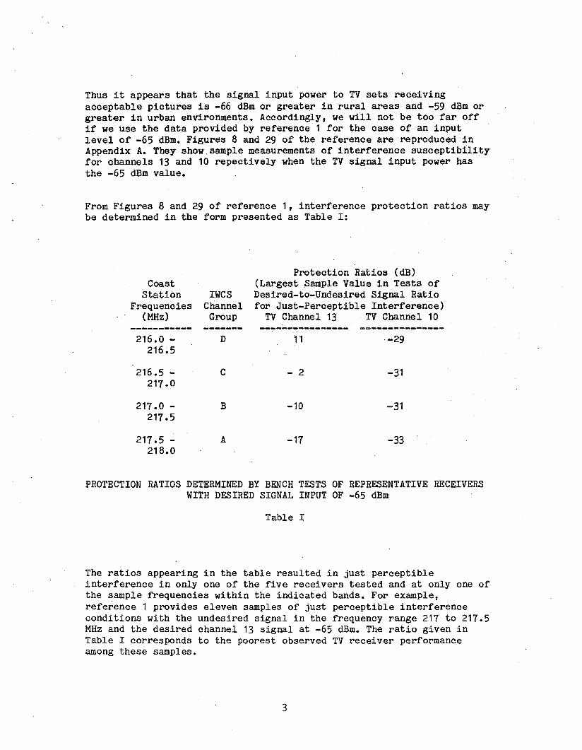
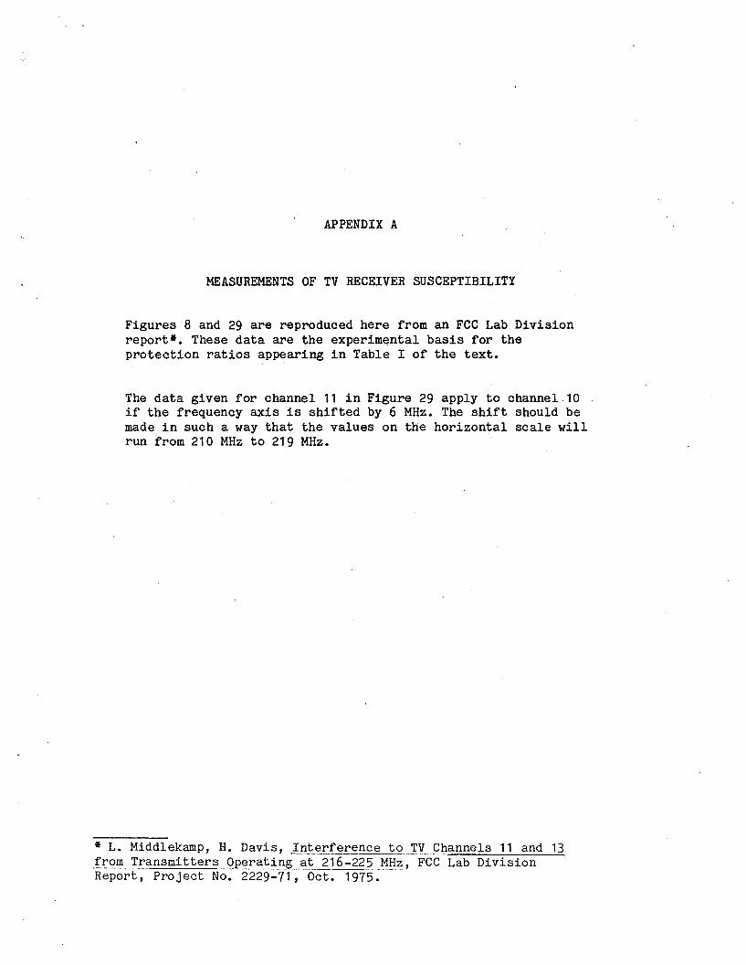
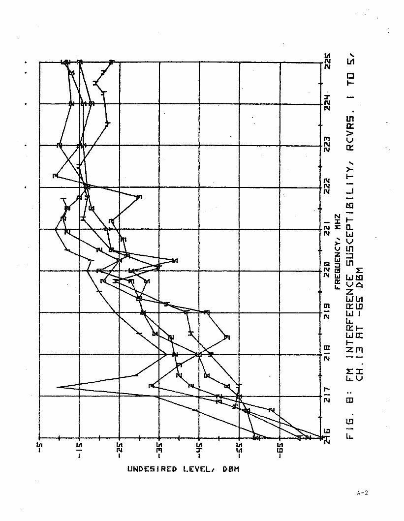
Thus it appears that the signal input power to TV sets receivingacceptable pictures is -66 dBm or greater in rural areas and -59 dBm orgreater in urban environments. Accordingly, we will not be too far offif we use the data provided by reference 1 for the case of an inputlevel of -65 dBm. Figures 8 and 29 of the reference are reproduced inAppendix A. They show sample measurements of interference susceptibilityfor channels 13 and 10 repectively when the TV signal input power hasthe -65 dBm value.

From Figures 8 and 29 of reference 1, interference protection ratios maybe determined in the form presented as Table I:

Protection Ratios (dB)Coast (Largest Sample Value in Tests of

Station IWCS Desired-to-Undesired Signal RatioFrequencies Channel for Just-Perceptible Interference)

(MHz) Group TV Channel 13 . TV Channel 10----------- ------- ---------------- ---------------216.0 - D 11 --29

216.5

216.5 - C - 2 -31217.0

217.0 - B -10 -31217.5

217.5 - A -17 -33218.0

PROTECTION RATIOS DETERMINED BY BENCH TESTS OF REPRESENTATIVE RECEIVERSWITH DESIRED SIGNAL INPUT OF -65 dBm

Table I

The ratios appearing in the table resulted in just perceptibleinterference in only one of the five receivers tested and at only one ofthe sample frequencies within the indicated bands. For example,reference 1 provides eleven samples of just perceptible interferenceconditions with the undesired signal in the frequency range 217 to 217.5MHz and the desired channel 13 signal at -65 dBm. The ratio given inTable I corresponds to the poorest observed TV receiver performanceamong these samples.

3

Since the number of measurements is quite small, the interferenceactually caused by IWCS stations may be more or less than that predictedby Table I. The table must be considered as providing a reasonable basisfor proceeding to develop these systems rather than assured criteria foravoiding interference. The five receivers measured represent a widerange of RF and IF circuits now in use. However, only one receiver ofeach type was observed.

RADIO PROPAGATION PREDICTION METHODAPPROPRIATE FOR IWCS INTERFERENCE TO TV

The propagation curves of FCC Report R-6602 [5] are recommended for thepurpose of predicting relative field strengths at various distances fromTV and IWCS stations. These curves are a~cepted standards fordetermining the potential for interference between TV services, makingthem very appropriate for the present related application. They areincorporated in the FCC's Rules for broadcast services. and are thereforefamiliar to engineers and operators of TV stations who may wish toreview IWCS engineering plans. The curves were developed by an extensivestudy of p~opagation measurements that had been made by both industryand gover.nment agencies. For the usual propagation modes in the VHF bandof concern here they still represent the most up-to-date information.

For convenience, the R-6602 curves related to channels 10 and 13 areincluded here as Appendix B. There are two sets, one predicting fieldstrengths that will be medians with respect to both receiver locationand. to variation in time, and the other for field strength exceeded for10% of the time at median locations. The symbols used to denote thesefields are F(SO,50) and F(50,10). Values of field strength exceeded for90% of the time may be obtained by assuming that the time fading followsthe normal or Gaussian type of distribution, with symmetrical variationabout the median level.

FIELD STRENGTH RATIOS AFFECTING THE INTERFERENCE POTENTIAL

The potential for interference at a geographical point .can be evaluatedin terms of the median fields there after making allowance for likelydeviations. Necessary considerations are (1) the variations in strengthof the competing electromagnetic fields with respect to location, (2)similar variations with respect to time and (3) the minimum acceptableratio between the two fields.

[~] J. Damelin, W. Daniel, H. Fine and G. Waldo, Development of VHF andUHF Propagation Curves for TV and FM Broadcasting, FCC, Office of ChiefEngineer, Research Div. Report No. R-6602, September 1966.

4

Location variability affects both the IWCS and the TV field. Medianvalues of these fields can be determined at any geographical point bythe p~opagation curves of Appendix B, and the relative strengths ofthese fields are a first indication of the interference potential.However, the situation will be considerably worse if the terrain of therespective propagation paths results in a stronger than average IWCSsignal or a weaker TV signal or both. This variability from location tolocation is usually assumed to have a Gaussian probability distributionwhen expressed in units of decibels (a log-normal distribution). It isgraphed in Fig. 1 of reference 2 and in Fig. 5 of ~eference 3. Thestandard deviation is about 8.6 dB, and there isa 90% chance that thedeviation will be as high as 11 dB.

At any particular TV reception point the fields.will also vary in time,and Appendix B includes information on the amount of such variations.The most reasonable method of combining the fading factors of the twofields is calculation of the square root of the sum of the squares (RSS)since both distributions are approximately log-normal and there is noapparent mechanism which would cause them to be correlated. Further, theTV reception point of concern will usually be relatively close to theIWCS station and far from the TV broadcasting tower with the consequencethat the fades in the· TV signal will be the dominant factor and the RSSfade will be approximately equal to that of the TV signaialone.

The minimum acceptable ratio between the two fields is analogous to thesignal ratios of Table I. We will assume that the ratio of fieldstrengths is converted into an equal ratio of input signals to the TVset. This ignores the possible advantage'of polarization discriminationby the antenna. Such advantages may not be justifiable since it is known[6J that the relative response of TV receiving antennas to horizotallyand vertically polarized waves is greatly dependent upon the relativebearings of the signal sources.

EVALUATION OF THE INTERFERENCE POTENTIAL

We seek criteria for identifying any geographical areas within whichthere is a reasonable likelihood of interference to TV. Reference 3includes a discussion of the approach used to determine adequateseparation distances between TV stations, and the same consid'er;:itionsare applicable here. Time and location'variability are treatedseparately in this approach. The objective is to determine thepercentage, L, of locations at which there will be interference-freereception at least T% of the time.

[6] A.C. Wilson, Performance of VHF Receiving Antennas, National Bureauof Standards Report 6099, May 26,1960.

5

Quantities involved in the analysis may be denoted by the followingsymbols (as in reference 3):

A= Minimum Acceptable Desired-to-Undesired Ratio; in dB,between the Fields.

Rd(T).= Time Distribution Factor, in dB, used to evaluate thedepth of fade affecting the desired signal at most T%of the time. Defined a~ Fd (50,T) - Fd(50,50) where thesubscript d refers to the desired field.

Ru(T) = Time Distribution Factor, dB, describing the amountby which the undesired field may increase during as muchas T% of the time. Defined as Fu(50.,T) - Fu(50,50)where the subscript u refers to the undesired field.

~Rd2(T)+Ru2(T) = Total Allowance, dB, for Variationswith Respect to Time.

The desired condition of no interference will hold where there is afavorable margin between the·TV signal and IWCS signals. In addition,there will be no interference in areas where the TV signal by itself istoo weak for reception. It fol~ows that the percentage, L, of locationswithout interference depends upon (1) the difference between medianfield strengths after the above allowances are made and also upon (2)the median field strength itself of the TV signal. The percentage L canbe determined from the following equation:

R(L,G) = A + Pu - Pd + Fu(50,50) - Fd(50,50)

+/Rl(T) + Ru2(T)

where

Pd = Effective Radiated Power (ERP) of TV Station,in dB above 1 kilowatt radiated from a half-wave dipole

Pu = ERP of IWCS Station (same units as Pd),

Fd(50,50) and Fu(50,50), in units of dB(uV/m), are median fieldstrengths that may be determined from Appendix B.

Fs = Minimum TV Field Strength for Service, in dB(uV/m). Forchannels 10 and 13 an appropriate value is 56 dB(uV/m),the level which defines the Grade B contour.

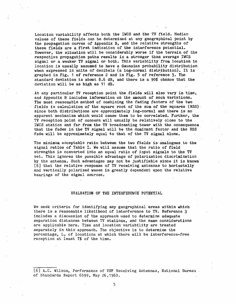
The function R(L,G) is graphed in Figure 1. It is derived fromprobability considerations in Appendix C.

6

,..

-L..:. +G 10 ±tti:~: ,. ,t-T­

., 1

I I" :..1-\I I

I'

,I II

-5

,~, , ~:::

:1=0: ~+5 ±t±1jj 0

!. I '.

-+T-1': 1 'j

!:' ., I

r:s Large~~ G

20

H++\J,:'I .1'I ,• I·, I

, I.

' ..

* 1 ,

.," 1;.

':,

1. I . 1 II

I! Ill'

1 I',:,1

I , 'II;

R(L, G) I 1 1·;I ·1,1 I

0, ,I

in dB , 1 1"'I:,, I ; Ij

,-!-,

,1 , 1'01.

: I , ,I

,- 1 :1 ,,

: , I II ,

~ I I

! I I'

. I l

• I"ii.:.

, "-1~;.C.·~~.: :,'II I _ IIIoLl!I:I~.

.• -~~ "~"-i~

xe.;..:~··, .~'1"'"

.x~_~~_

I 1 I

! I I Iill 1 I

': :

! I'

I ~_i.-

. I j I I:

, ,I: "

I I

;-~ i;;·

'I, !

' ..

. i'.

1 "

j.

: ! .•I I! •

;:

I 1, ,

I , , : ,1 I :,.,.

: , II , I 1, , I

: ,-,:~~~j. I [I !:'

•• *.~I ._[

10

-10

,. ,

9895

; I

• I

Ii j1 ,

90

II I, I

• I

;, :',;1

,!",

80

1 I• : t ,

: I' •

; t I I

, I'I I

'I' ;

" ,

,'I I

,I i;I '!;

:. I, I'

, ..

60 70

': 'I.

!' ..

-" '" 1

,;; I:

l' I

40 50

;: ,'!

30

1 •, :

II,

I I' ;

1 I

I Ii;;. ;;' I.

~-

I'

, ~;-f-'.-:-10 20

_1- ....

2 5

-20

Percent, L, of Locations

L is the percentage of locations atsignal by itself is too weakdesired-to-undesired field ratio isamount at least equal to R(L,G).

which either (1) the desiredfor reception or (2) thehigher than its median by an

For example, suppose that the median desired-to-undesired ratioin the area of interest is 6 dB higher than the value needed toavoid interference. Then R(L,G) can be as low as -6 dB. If it isalso supposed that the area' is near the Grade B contour whereG=O, then 95% of locations will be without interference sinceR( 95, 0) = -6.

GRAPH OF FUNCTION R(L,G) WHICH MAY BE USED TO DETERMINEPERCENT OF LOCATIONS WITHOUT INTERFERENCE

Figure 1

7

DETERMINATION OF THE INTERFERENCE CONTOUR

At a later time it may become possible to choose the percentages T and Lon the basis of actual experience with IWCS stations operating near TVservice areas. At present it appears reasonable to use 90% for bothvalues. Television grades of service are specified with reference to 90%of the time, and it is consistent to use T = 90% in evaluatinginterference also. There is related experience in other applications. InparticUlar, the use of a 90% time and location reliability criterion hasbeen successful as a practical matter in the Domestic Public Land MobileRadio Service for establishing interference contours [7].

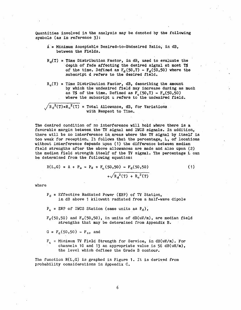
The interference contour will be the set of geographical points at whichequation (1) is satisfied with the suggested levels of time and locationreliability. The area of potential interference may be considered aslying inside. The prediction for this area is that the followingconditions will both be found at more than 10% of locations: (1) Thedesired TV signal by itself WOUld. be adequate at least 90% of the time,but (2) the ratio between desired and undesired fields is unacceptablemore than 10% of the time.

Figure 2 will help locate the interference contour. The Figure is agraph of -R(L,G) which may be considered as a component of a margin tobe imposed between desired and undesired fields. Equation (1) issatisfied wherever the desired and undesired signals differ by the totalmargin found by adding the appropriate value read from the figure to themargin A +/R u

2 (10) + R/(10).

For example, Grade B service of a maximum facility TV station in Zone I(1000-foot antenna, 316 kilowatts) extends 60 miles from the station andRct (10) for this distance is 7 dB (see Appendix B). The total requiredmargin in dB is:

=and the IWCS field strength may be as great as 56 dB(uV/m) (the medianTV field strength at the Grade B contour) less this margin. That is, theIWCS field strength (50% of lo~ations, 50% of time) along this contourshould not exceed 54.4 - A -VR u

2(10) + 49 dB(uV/m). If the IWCS fielddoes exceed the upper limit calculated in this way, or if the proposedstation lies inside the Grade B contour, these calculations must berepeated at other TV service contours (higher median field strengths andcloser to the TV station) to determine the area of potentialinterference. No further analysis is required for stations lying outsideand providing sufficient margin at the Grade B contour.

[7] R.B. Carey, Technical Factors Affecting the Assignment ofFacilities in the Domestic Public Land Mobile Radio Service, FCC ReportNo. R-6406, Washington, D.C., June, 1964.

8

1 0 H--H-++-t-!"++-+-+-+-1-+-1f-t-1H-H-H-H-f+-bl"++++++++++++-+-+++-+-+++-H

Additional II·I 1/

Margin 0JT

I ;

i n dB

,.....,-.,

-10

, 1I./

./I I II, :

I

-20 I

-'-- ....

i-+-~-~

-+:-J~--i-:-~.

I I I .:I-----~

1

-10 0

I ,- Ii"

10 20

, I

J I .

I I

30

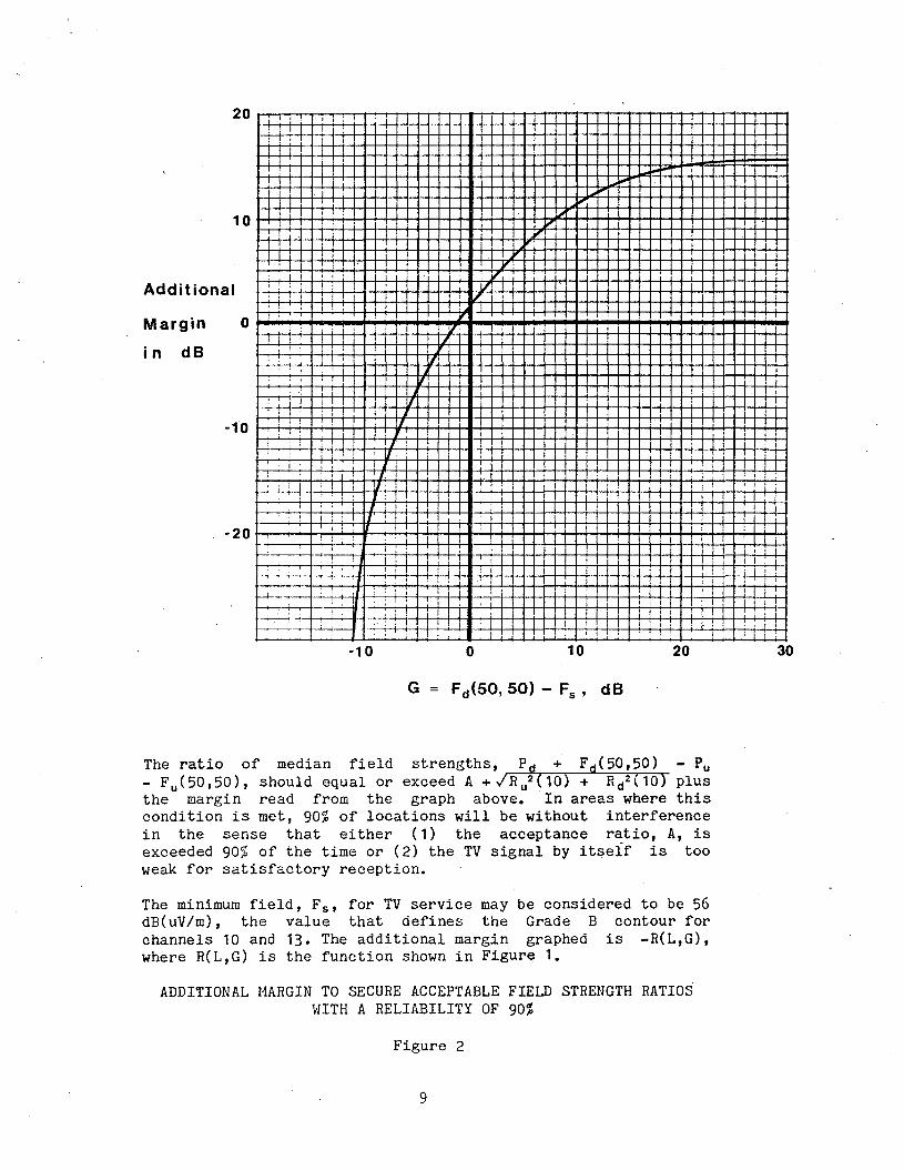
The ratio of median field strengths, Pd + Fd (50,50) - Pu- Fu (50,50), should equal or exceed A +JR u2(10) + Rd2(10) plusthe margin read from the graph above. In areas where thiscondition is met, 90% of locations will be without interferencein the sense that either (1) the acceptance ratio, A, isexceeded 90% of the time or (2) the TV signal by itseif is tooweak for satisfactory reception.

The minimum field, Fs , for TV service may be considered to be 56dB(uV/m), the value that defines the Grade B contour forchannels 10 and 13. The additional margin graphed is -R(L,G),where R(L,G) is the function shown in Figure 1.

ADDITIONAL MARGIN TO SECURE ACCEPTABLE FIELD STRENGTH RATIOSWITH A RELIABILITY OF 90%

Figure 2

9

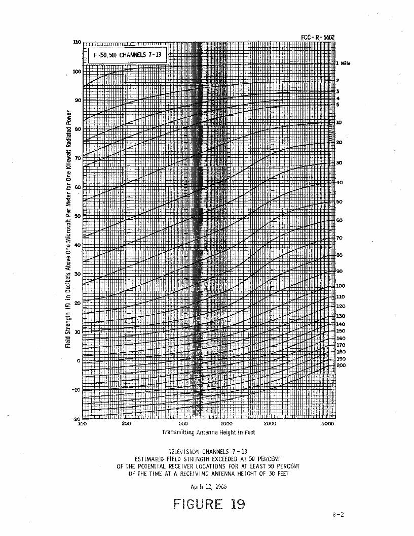
For example, suppose it is desired to operate an IWCS station 10 milesfrom the Grade B contour of a channel 13 TV station. Suppose in additionthat the proposed frequency of operation is from IWCS Channel Group B sothat A = -10 as determined by Table I. As far as 20 miles away it isfound (Figure 10 of Appendix B) that Ru (10) is less than 2 dB. As aresult the precise value of Ru(10) does not affect the computationsexcept somewhat beyond 20 miles. Within this range and along the Grade Bcontour the IWCSfield may be as large as

54.4 - A -/R/(10) + 49 == 57.4 dB(uV/m).,

Now refer to Figure 19 of Appendix B and assume that the proposedstation will have an antenna height of 200 feet. If the ERP is 1kilowatt, the propagation prediction curves can be read directly. Thecurves predict that the IWCS field will fall to the acceptable level of57.4 dB(uV/m) at a distance of about 12.5 miles, somewhat inside theGrade B contour. If the ERP is reduced to about 440 watts, the~nterference contour will just touch the' Grade B leaving no overlap,which may be considered an acceptable situation.

SPECIFIC SITUATIONS REQUIRING INTERFERENCE STUDIES

Present FCC rules require that IWCS applications include an engineeringplan for suitable limiting of the interference contour when any of thefollowing conditions apply:

• The station as proposed will have an antenna height greaterthan 200 feet (61 meters), or

• the proposed station is located less than 105 miles(169 kilometers) from a channel 13 TV station, or

• it is located less than 80 miles (129 kilometers) froma channel 10 station.

The interference contour is defined to include only areas inside thetelevision Grade B contour. The later lies where the TV field strength(for the channels of concern here) is 56 dB(uV/m), and this is to bedetermined as follows using the F(50,50) curves:

• For broadcast stations, maximum permissible TV antennaheight and power are to be assumed. Appendix D, includedhere for convenient reference, provides information on thesemaximum values.

• For translators and low power TV stations, use the actuallylicensed antenna height and power.

10

ACCEPTABLE FORMATS FOR PRESENTATION

The engineering plan is to include a delineation of the interferencecontour, identification of the method used to determine the contour, anda statement concerning the number of residences inside. The methodshould be based on technical considerations equivalent to thosepresented in this report. When the purpose is to demonstrate the absenceof potential interference problems, worst case assumptions may be usedto simplify the calculations.

The following are examples of methods of presenting interference studyresults. They are recommended as efficient ways to make the necessarydemonstrations.

Case 1.

Situation:Proposed station is located outside the Grade B TV contour, and theproposed radiation pattern is omnidirectional.

Demonstration that Interference Potential is Minimized:At the point where the direct line connecting the two stationsintersects the Grade B, show the F(SO,SO)-values of the respectivefields. Compare with the value of the minimum margin by which theTV field should exceed that of the IWCS signal at this point, andshow how this margin has been determined. The comparison, ofcourse, must be favorable.

Remarks:When it can be used, this analysis is preferred because of itssimplicity. If the radiation pattern is not omnidirectional, it maybe convenient to make a worst-case assumption that a maximum ofeffective radiated power is directed at the TV station. Thesituation may then be treated as if this maximum were beingradiated in all directions.

Case 2.

Situation:Proposed station is located outside the Grade B contour, and theproposed radiation pattern is directional.

Demonstration that Interference Potential is Minimized:Tabulate the F(50,SO)-values of the two fields along anappropriately extensive segment of the Grade B contour. Include inthe tabulation the minimum acceptable margin at each Grade B point,and identify the method used to determine these margins.

Remarks:Tabulate as a function of azimuth around the proposed station. Use

11

a fine enough spacing to make it apparent approximately where thepoint of maximum interference lies.

Case 3.

Situation:Proposed station is outside the Grade B, but the interferencecontour penetrates the TV service area.

Presentation of Interference Study Results:In this case it will be necessary to describe the interferencecontour. It appears most convenient to tabulate the pertinentquantities as a function of azimuth around the proposed station,starting and ending at the points where the interference contourcrosses the Grade B. At each bearing, give the distances to theGrade B and to the interference contour to indicate the size of theincluded area. At each bearing show also the desired and undesiredF(SO,SO)-values of field strength and the minimum acceptablemargin.

Remarks:The increment between successive bearings tabulated should be smallenough so that the general shape of the area of potentialinterference is described. This is more or less critical dependingupon the population density of the area overlaid.

Case 4.

Situation:Proposed station lies inside the Grade B contour.

Presentation of Interference Study Results:Same as Case 3 except that consideration will have to be given toconditions in every direction around the proposed station.

The foregoing examples have outlined the information which is logicallynecessary to make the required demonstrations. Applications willpresumably also provide supporting data such as geographical coordinatesof the stations, antenna heights, antenna radiation pattern and theproposed ERP in the direction of maximum power.

12

APPENDIX A

MEASUREMENTS OF TV RECEIVER SUSCEPTIBILITY

Figures 8 and 29 are reproduced here from an FCC Lab Divisionreport*. These data are the experimental basis for theprotection ratios appearing in Table I of the text.

The data given for channel 11 in Figure 29 apply to channel 10if the frequency axis is shifted by 6 MHz. The shift should bemade in such a way that the values on the horizontal scale willrun from 210 MHz to 219 MHz.

* L. Middlekamp, H. Davis, Interference to TV Channels 11 and 13from_!ransmitters Operating at_ 216-225 MHz, FCC Lab DivisionReport, Project No. 2229-71, Oct. 1975.

~ "N 111N

CI-

:rNN

U1D::>

1"1 VN a:N

">-N l-NN ...J

toN I-:I:

N J: Q.N W... v>-v U1z :::Jm W III.:JNe 1:NW WtOa::: VOla.

ZWLt1

D'1 0':1.0- WIN L..0':1-Wa:-ן

m Zf11-N1::I:u..V

,...-N []]

l!l-u....... ltI ..... ..... IJI lttI - N 1"1 :r .....

I I I I I

UNDESIRED LEVEL, DSM

A-2

111 "N lJ1N

0·....f11

:r --NN oJ:

UlV0::>...J

PI VWN 0::>NW

"...J>-

"I .... -N -...JN ...Je:

-::::1tO~

N -W-:I: .... -"IS:: 0-N WJ:,

Vr->-V Ul-z ::::1:3:

I5IW Ul

N::J %:Nfl Wt£1a: VOla.

ZWlJ1

D1 O::LD- WIN La..0:: ....We:....m z--N1:J:La.. V

,..."I D1

N

l!JLD

La..-111 111 111 111 111 IJt 111 NI - "I P1 :r 111 LD

I I I I I I

UNl>ESIREl> LEVEL, l>BH

A-3

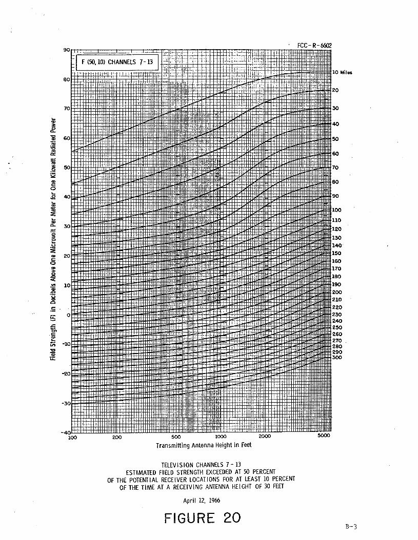
APPENDIX B

PROPAGATION CURVES

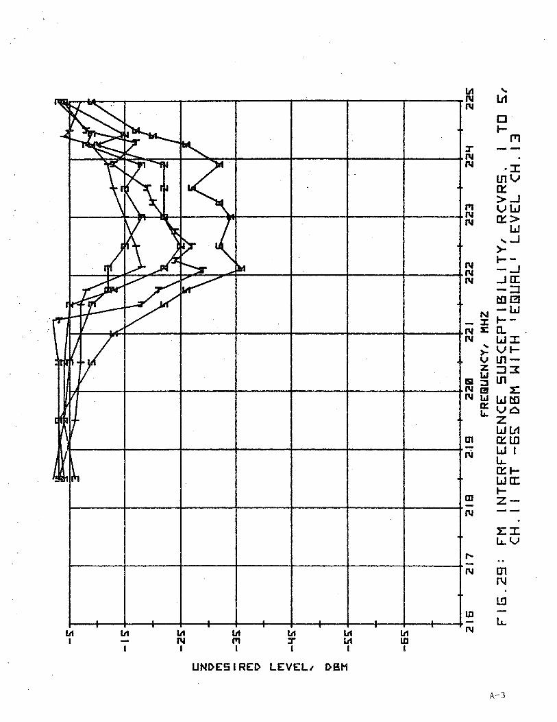
Propagation prediction curves appropriate for evaluating thepotential for IWCS interference to television are reproducd herefor convenience. The curves are from FCC Report R-6602*.

The fading margin values given in Figure 10 are derived from theother two figures simply by subtraction. In the text thisdifference,

F(50,10) - F(50,50)

is denoted by Rd (10) or Ru (10) where the subscripts d and urefer to the desired and undesired signals respectively.

* J. Damelin, W. Daniel, H. Fine and G. Waldo, Development of VHFand UHF Propagation Curves for TV and FM Broadcasting, FCC, Officeof Chief Engineer, Research Div. Report No. R-6602, September1966.

I', '

:rr;:""

500 1000 2000

Transmitting Antenna Height in Feet

200

-10

-20100

F.CC-R,-~

·1F 00, SO) CHAN'NELS 7-13 I,

I Mil.

100

2

3

90 45...

G>

~ 10

15 801ii:;:;

2010ex:;g~ 70

5230

G>C0... 40.E 60...G>

1i> 50:E...G>Q. 50- 60geu~ 70G> 40c0 80G>>.8<: 90'" 30Q).c~ 1000 ~ ..J~

C

u: 20

.t::.en ..c " ~:: 140G>...- lO ' 150en

"t:> ": 160Qi riu: 170

: 1800

...190

: 200

TELEV ISION CHANNELS 7 - 13ESTIMATED FIELD STRENGTH EXCEEDED AT 50 PERCENT

OF THE POTENTIAL RECEIVER LOCATIONS FOR AT LEAST 50 PERCENTOF THE TIME AT A RECEIVI NG ANTENNA HEI GHT OF 30 FEET

Aprii 12, 1966

FIGURE 19B-2

10 Miles

5000500 1000 2000

Transmitting Antenna Height in Feet200

-I F (50, 10) CHANNELS 7- 13

80

-30

-40100

70

....Q)

~~ 60-co'i5co0:::

i6~ 50

~Q)

C0....,g 40....Q)

Q;:E....Q)Q.. 30-g ,0

':

....U

:EQ) 20c0Q)

>.8<C

'" 10. rl

~.~

Q

C

u::: 0,.

"

.c,+t,

t:n ".C

Q)....- -10VI'0Qiu::

-20

TELEVISION CHANNELS 7-13ESTIMATED FIELD STRENGTH EXCEEDED AT 50 PERCENT

OF THE POTENTIAL RECEIVER LOCATIONS FOR AT LEAST 10 PERCENTOF THE TIME AT A RECEIVING ANTENNA HEIGHT OF 30 FEET

April 12, 1966

FIGURE 20B-3

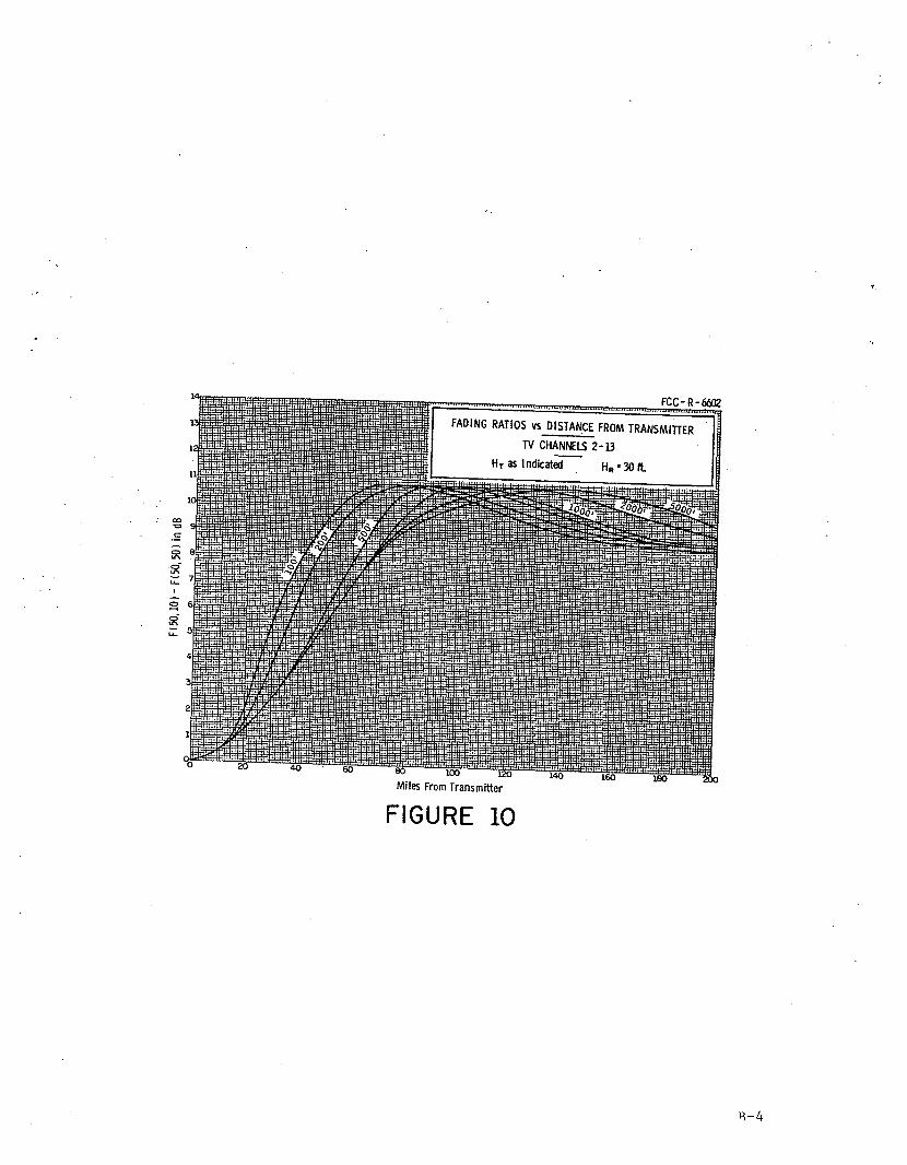
FCC;' R-6602

FADING RATiOS vs DISTANCE FROM TRANSMITIER

TV CHANNELS 2-13-HT as Indicated HR' 30 tt.

FIGURE 10

1)-4

-APPENDIX C

JOINT PROBABILITY CONSIDERATIONS FOR PREDICTION OF

THE RELATIVE NUMBER OF LOCATIONS WITHOUT INTERFERENCE

It is reasonable that interference protection criteria should vary withthe grade of service being protected. In the case of interference fromanother television station, the traditional approach requires that theminimum acceptable ratio between fields be present at L% of locationswith L = 70% at the Grade A contour and 50% at the Grade B. Thesepercentages are the same as those which define the contours in terms ofcoverage. At the limit of Grade B service, for example, it is expectedthat TV reception will be available to 50% of residences on the basis ofthe desired field strength alone. If there is an additional signal from adistant co-channel station, it is considered appropriate to apply asimilar 50%-of-Iocations criterion to the ratio of the two televisionfields.

It is necesary to examine the possibilities for lWCS interference to TVin greater detail since it would be unacceptable to cause interferenceto as many as 50% of residences in densely populated areas. IWCSoperators are required to eliminate harmful TV interference that theirstations cause within Grade B contours. This might be impractical if alarge number of TV sets were involved.

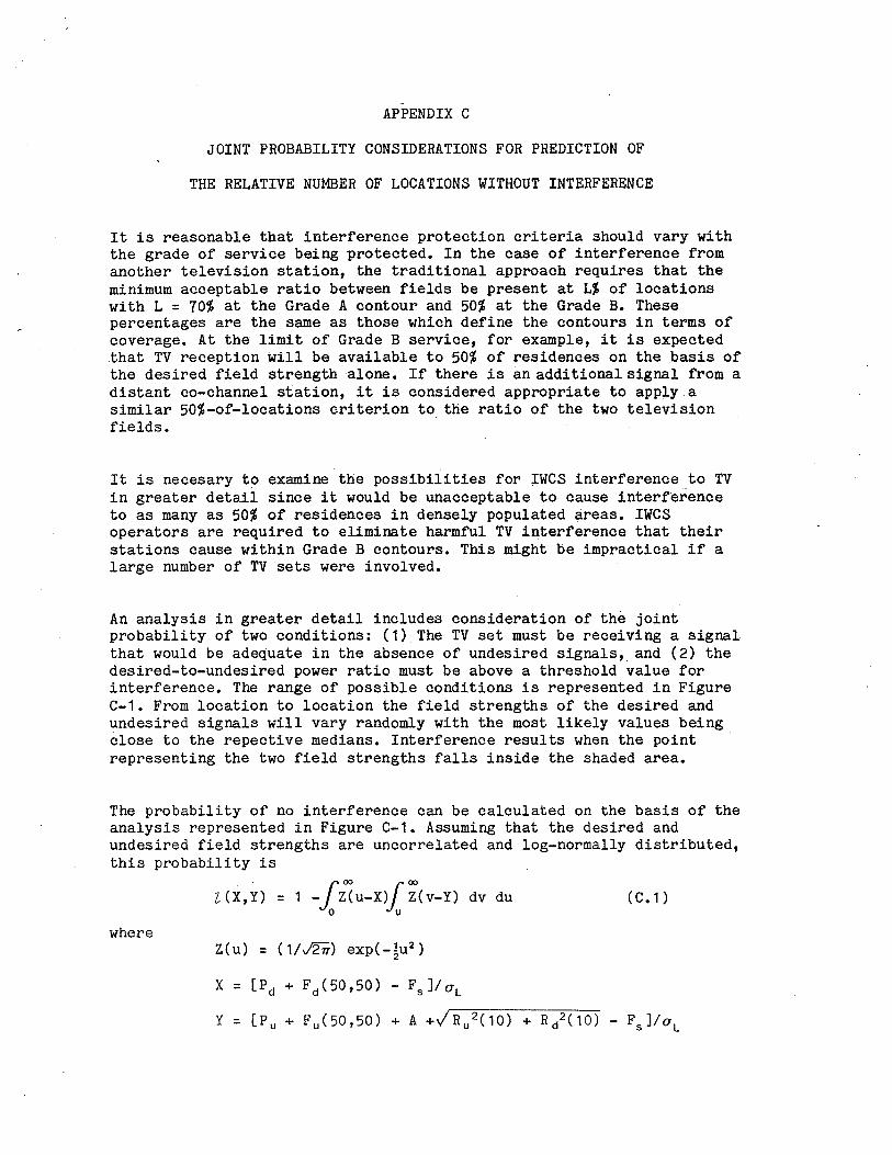
An analysis in greater detail includes consideration of the jointprobability of two conditions: (1) The TV set must be receiving a signalthat would be adequate in the absence of undesired signals, and (2) thedesired-to-undesired power ratio must be above a threshold value forinterference. The range of possible conditions is represented in FigureC-1. From location to location the field strengths of the desired andundesired signals will vary randomly with the most likely values beingclose to the repective medians. Interference results when the pointrepresenting the two field strengths falls inside the shaded area.

The probability of no interference can be calculated on the basis of theanalysis represented in Figure C-1. Assuming that the desired andundesired field strengths are uncorrelated and log-normally distributed,this probability is

z<X, Y) = 1 -fz<u-X)f ~(v-Y) dv du (C.no u

whereZ(u) = (1/v2rr) exp(-~u2)

X = [Pd + Fd (50,50) - Fs]laL

y = [P u + Fu (50,50) + A +/R u2 (10) + R/(10) - Fs]la L

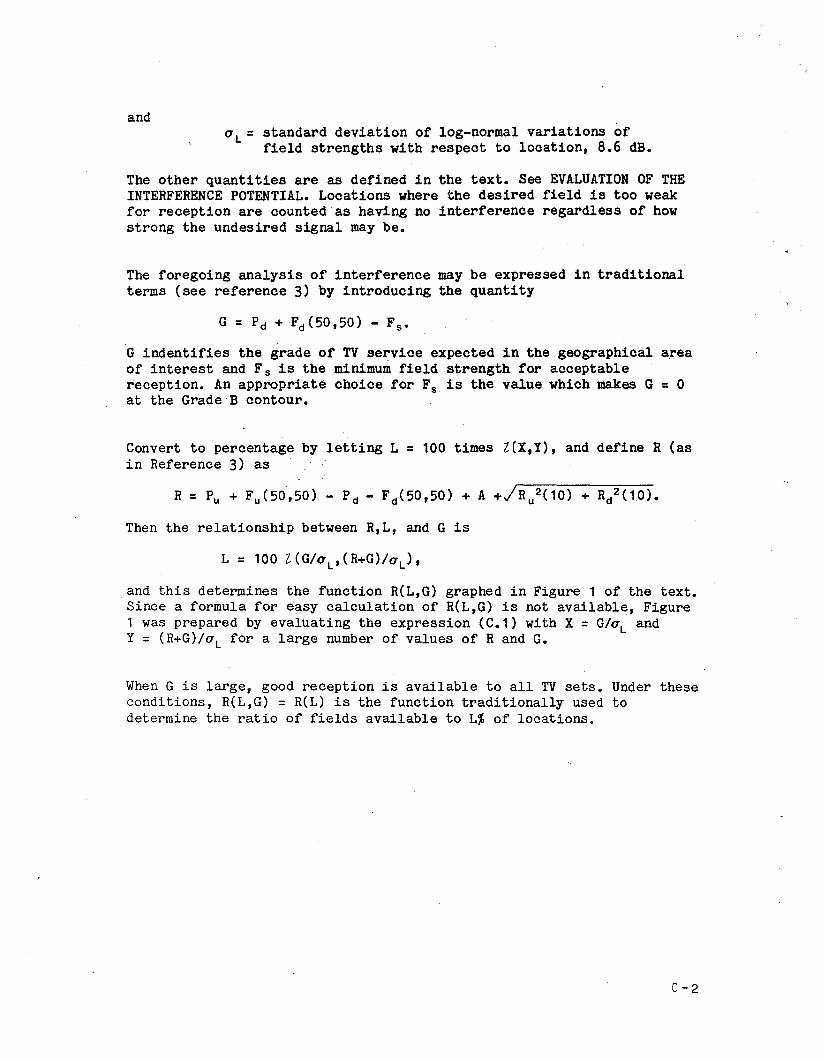
and0L =standard deviation of log-normal variations of

field strengths with respect to location, 8.6 dB.

The other quantities are as defined in the text. See EVALUATION OF THEINTERFERENCE POTENTIAL. Locations where the desired field is too weakfor reception are counted as having no interference regardless of howstrong the undesired signal may be.

The foregoing analysis of interference may be expressed in traditionalterms (see reference 3) by introducing the quantity

G indentifies the grade of TV service expected in the geographical areaof interest and F s is the minimum field strength for acceptablereception. An appropriate choice for Fs is the value which makes G =0at the GradeB contour.

Convert to percentage by letting L =100 times l(X,Y), and define R (asin Reference 3) as

R = Pu + Fu (50,50) - Pd - Fd (50,50) + A +JR u2(10) + Rl(10).

Then the relationship between R,L, and G is

and this determines the function R(L,G) graphed in Figure 1 of the text.Since a formula for easy calculation of R(L,G) is not available, Figure1 was prepared by evaluating the expression (C.l) with X = G/oL andY = (R+G)/oL for a large number of values of Rand G.

When G is large, good reception is available to all TV sets. Under theseconditions, R{L,G) = R(L) is the function traditionally used todetermine the ratio of fields available to L% of locations.

C-2

Undes iredFieldStrengtdB (uV/m)

Median ofUndes ired

Fie ld

Bi-variate log-normaldistribution of

@-f.ieldstrengthS

L:\ centered- - - \1J here.

I

II

Strength of

Hinimum Accept­able Ratio be­

tween Fields

t

/ Min imum Fie 1d/ for Acceptable,-

Reception

Median ofDesired Field

Des I re IedB(uV/m)

The relationships illustrated above are the basis for theprobability-of-interference evaluation used in this report.Field strengths are represented logarithmically, and theintersection of the x- and y-axes is an arbitrarily chosenreference at which the two fields are equaL

Interference occurs when (1) the desired field is strong enoughfor reception and (2) the field strength ratio does not provideenough protection.

GRAPHICAL ANALYSIS OF RECEPTION AND INTERFERENCE CONDITIONS

Figure C-1

C-3

APPENDIX D

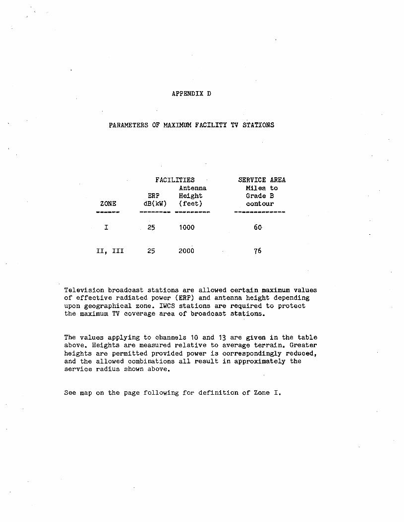
PARAMETERS OF MAXIMUM FACILITY TV STATIONS

FACILITIES SERVICE AREAAntenna Miles to

ERP Height Grade BZONE dB(kW) (feet) contour

------ -------- --------- -------------I 25 1000 60

II, III 25 2000 76

Television broadcast stations are allowed certain maximum valuesof effective radiated power (ERP) and antenna height dependingupon geographical zone. IWCS stations are required to protectthe maximum TV coverage area of broadcast stations.

The values applying to channels 10 and 13 are given in the tableabove. Heights are measured relative to average terrain. Greaterheights are permitted provided power is correspondingly reduced,and the allowed combinations all result in approximately theservice radius shown above.

See map on the page following for definition of Zone I.

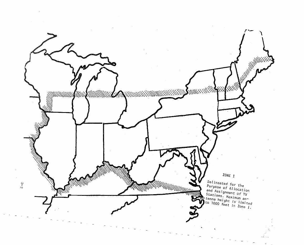
t::;)I

N

ZONE I

Delineated for thePurpose of Allocat ionand ASSignment of TVStations. Maximum an~

- A tenna hei ght is' I imi ted~ to 1000 feet ;n Zone 1.~